JOB DISPLACEMENT AND THE DURATION OF JOBLESSNESS:

THE ROLE OF SPATIAL MISMATCH

by

Fredrik Andersson *Office of the Comptroller of the Currency

John C. Haltiwanger *University of Maryland and U.S. Bureau of the Census

Mark J. Kutzbach *U.S. Bureau of the Census

Henry O. Pollakowski *Harvard University

and

Daniel H. Weinberg * RetiredU.S. Bureau of the Census

The research program of the Center for Economic Studies (CES) produces a wide range of economic analyses to improve the statistical programs of the U.S. Census Bureau. Many of these analyses take the form of CES research papers. The papers have not undergone the review accordedCensusBureaupublications and no endorsement should be inferred. Any opinions and conclusions expressed herein are those of the author(s) and do not necessarily represent the views of the U.S. Census Bureau. All results have been reviewed to ensure that no confidential information is disclosed. Republication in whole or part must be cleared with the authors.

To obtain information about the series, see www.census.gov/ces or contact Fariha Kamal, Editor, Discussion Papers, U.S. Census Bureau, Center for Economic Studies 2K132B, 4600 Silver Hill Road, Washington, DC 20233, CES.Papers.List@census.gov.

This paper is a revised version of JOB DISPLACEMENT AND THE DURATION OF JOBLESSNESS: THE ROLE OF SPATIAL MISMATCH(CES-WP-11-30) from

September 2011. Acopy of the original paper is available upon request.

CES 11-30R April, 2014

Abstract

This paper presents a new approach to the measurement of the effects of spatial mismatch that takes advantage of matched employer-employee administrative data integrated with a person-specific job accessibility measure, as well as demographic and neighborhood characteristics. The basic hypothesis is that if spatial mismatch is present, then improved accessibility to appropriate jobs should shorten the duration of unemployment. We focus on lower-income workers with strong labor force attachment searching for employment after being subject to a mass layoff – thereby focusing on a group of job searchers that are plausibly searching for exogenous reasons. We construct person-specific measures of job accessibility based upon an empirical model of transport modal choice and network travel-time data, giving variation both across neighborhoods in nine metropolitan areas, as well as across neighbors. Our results support the spatial mismatch hypothesis. We find that better job accessibility significantly decreases the duration of joblessness among lower-paid displaced workers. Blacks, females, and older workers are more sensitive to job accessibility than other subpopulations.

*

JEL Codes: J64, R23, R41. Keywords: spatial mismatch, job accessibility, competing searchers, modal choice, job search, unemployment duration, mass layoff events.

*Any opinions expressed in this document are those of the authors and do not necessarilyrepresent the views of the Office of the Comptroller of the Currency or the U.S. Census Bureau. All results have been reviewed to ensure that no confidential information is disclosed. The authors thank the discussants and participants at numerous seminars and conferences for their comments on earlier versions of this research, including the Urban Economics Association (2010), the American Real Estate and Urban Economics Association/Allied Social Sciences Association (2011), the Urban Economics Association (2011), the Society of Labor Economists (2012), the Census Bureau Center for Economic Studies (2012), and the Federal Reserve Bank of Atlanta Comparative Analysis of Enterprise Data Conference (2013). We also are thankful for early comments on this research from Kevin McKinney and Ron Jarmin. We also thank Sheharyar Bokhari for significant assistance with the transportation network data and modeling. This research uses data from the Census Bureau’s Longitudinal Employer-Household Dynamics (LEHD) Program, which was partially supported by the following grants: National Science Foundation (NSF) SES-9978093, SES-0339191 and ITR-0427889; National Institute on Aging AG018854; and grants from the Alfred P. Sloan Foundation. The research for this project was also supported by a grant from the MacArthur Foundation.

Job Displacement and the Duration of Joblessness: The Role of Spatial Mismatch

I. Introduction

The spatial mismatch hypothesis (SMH) encompasses a wide range of research questions,

all focused on whether a worker with locally inferior access to jobs is likely to have worse labor

market outcomes. The literature grew out of two papers by Kain (1964, 1968), which proposed

that persistent unemployment in urban black communities might be due to a movement of jobs

away from those areas, coupled with the inability (due to housing discrimination) for those

residents to relocate closer to jobs. One corollary of this hypothesis is that improving spatial

access to jobs would lead to better outcomes. In addition to broad national policies aimed at

reducing housing discrimination, this logic has inspired urban planning policies aiming to (1)

move jobs closer to neighborhoods with high unemployment, as is intended with Employment

Zones (Neumark and Kolko 2010); (2) enhance transportation links between high unemployment

neighborhoods and locations with an abundance of jobs, as is done with transit expansions

(Holzer et al. 2003); and (3) relocate residents of high unemployment neighborhoods to job-

abundant neighborhoods, as might occur with a housing voucher program (Katz et al. 2001).

Despite these well-intentioned policies, continued urban concentrations of lower-income

and minority populations continue to have higher than average unemployment rates. Study of the

SMH thus remains highly relevant while there nonetheless remains uncertainty about its relative

importance. Glaeser (1996) and others have pointed out that cross-section models omit

unobserved person characteristics that may be correlated with neighborhood location as well as

employment outcomes. This phenomenon may bias impact estimates of job accessibility that rely

on neighborhood-specific effects, though the degree to which it biases cross-section outcomes is

open to question.

This paper presents a new approach to the measurement of the effects of spatial

mismatch. We address several outstanding issues in the literature, with an emphasis on

identification strategies that mitigate the impact of (endogenous) residential self-selection.

Central to our approach to spatial mismatch is the ability to combine data sources to produce

improved, person- and location-specific measures of job accessibility.

2

Our results support the spatial mismatch hypothesis. We find that better job accessibility

significantly decreases the duration of joblessness among lower-paid displaced workers. This

result is strongest for non-Hispanic blacks, females, and older workers.

The remainder of this paper is organized as follows: Section II reviews the spatial

mismatch literature with a focus on identification issues. Section III presents our model and

identification strategy. Section IV describes the data, accessibility measures, and sample

construction. Section V presents our main estimation results along with the economic

significance of our findings and Section VI provides our conclusions.

II. Related Literature

“Spatial mismatch” was first described as a breakdown of the standard urban land use

model. Observing 1950s data, Kain (1964, 1968) found that the location of jobs for blacks was a

poor predictor of their residences. Kain’s argument was that racial discrimination in the suburban

housing market prevented central city blacks from moving to suburbs, where jobs were moving

to, driving up their unemployment rate (and also their rents). Thus, at the core of the SMH is job

accessibility, that is, distant jobs are more difficult to obtain due to high costs of search and

commuting (see, e.g., Brueckner and Zenou 2003).

Kain’s work has spawned a huge subsequent empirical literature, almost exclusively

focused on cross-section analysis, and most recently summarized by Kain (1992, 2004),

Ihlanfeldt and Sjoquist (1998), and Gobillon et al. (2007). Although the synthesis articles have

been critical of some work, there is nevertheless considerable evidence that poor job accessibility

is partially responsible for poor labor market outcomes for inner-city low-skilled ethnic

minorities. However, there is considerable disagreement about the magnitude of the spatial

mismatch effect and about which groups of workers are most affected by it (Ihlanfeldt 2006).

Arguably, much of the disagreement stems from limitations of the underlying data, which we can

better address in this paper due to detailed and comprehensive location-specific longitudinal

data.

A central problem for spatial mismatch research, highlighted by Ihlanfelt (1993) and

Glaeser (1996), among others, is the endogeneity of employment outcomes and residential

location. One approach to mitigate these problems is focusing on youth who live with their

parents (see Raphael 1998; O’Regan and Quigley 1996a, 1996b). However, if parents and

3

children share the same unobserved heterogeneity, then this approach mitigates but does not

solve the problem. In a related manner, measures of job accessibility that vary only by

neighborhood will tend to correlate with other neighborhood characteristics that may also be

relevant for labor market outcomes. Yet another problem highlighted by Ihlanfeldt and Sjoquist

(1998) is that job accessibility measures should control for the number of competing searchers.

Our new approach departs from the existing work that focuses on cross-sectional

variation by using longitudinal data on workers who have experienced an involuntary job

displacement. We argue that finding a job after a spell of involuntary unemployment is

exogenous to the previous residential location decision. That is, the mass layoff event per se is

the impetus for the job search, rather than local job opportunities. There is a substantial literature

in labor economics studying the impact of job displacement following the seminal paper of

Jacobson et al. (1993). Using matched employer-employee data for the state of Pennsylvania,

Jacobson et al. showed that workers separating from a sharply contracting employer experience a

substantial and persistent loss in earnings. A closely related literature has shown that separations

from a sharply contracting business are more likely to be associated with a layoff (an involuntary

separation) as opposed to a quit (see Davis et al. 2012 for a summary of this literature).

We are not the first to explore the role of spatial mismatch on job search duration. Studies

by Rogers (1997), Dawkins et al. (2005), Johnson (2006), and Gobillon et al. (2011) look at

search duration in this context and find that greater job accessibility reduces search duration.

Relative to this existing literature we make several contributions. In particular, this is the first

paper in this area to focus on workers displaced from a mass layoff, which is a critical aspect of

our identification strategy since it almost guarantees that these individuals have strong labor

force attachment and that residential location remains exogenous to the short-run re-employment

problem these workers face. Second, previous studies are based on relatively small samples of

workers without the information we exploit on job history and without the ability to control for

employer fixed effects. Third, most previous studies are for a single urban area or a small set of

cities, and often do not include suburban areas, while our study casts a much wider geographic

net.

Our research is also intended to address important issues raised by Houston (2005) and

others (e.g., Perle et al. 2002) about the proper measurement of job accessibility in testing the

SMH. Researchers have emphasized the importance of using commute times instead of distance

4

in measuring accessibility, accounting for local job competition, disaggregating job counts into

those most relevant for a searcher, and including locational characteristics.1 Raphael and Stoll

(2001) emphasize the importance of auto ownership. They find that having access to a car is

particularly important for blacks and Latinos. Several other studies also emphasize the

importance of vehicle ownership on finding employment, including Baum (2009), Ong and

Miller (2005), Johnson (2006), and Korsu and Wenglenski (2010). They all find that vehicle

ownership improves job accessibility. Our analysis incorporates both automobile and public

transit transportation modes.

III. Methodology and Empirical Strategy

We test for spatial mismatch by employing an empirical specification that relates duration

of joblessness to an index of job accessibility and other control variables. In this section we

demonstrate how our specification can be derived from a simple job search theoretic framework.

We also discuss how we address various econometric issues that can otherwise invalidate

inference.

A. Theoretical Motivation

Following closely the theoretical exposition in Rogerson et al. (2005), consider an

individual searching for a job in continuous time. This individual seeks to maximize the expected

value of �∫ 𝑦𝑡𝑒−𝑟𝑡∞𝑡=0 �, where 𝑟 𝜖 (0,1) is the discount factor, and 𝑦𝑡 is the income at 𝑡. Income is

𝑦 = 𝑤 − 𝑐 if employed with wages 𝑤 and commute costs 𝑐, and 𝑦 = 𝑏, if unemployed. To

introduce a spatial dimension, we depart slightly from the standard job search model that

assumes that job offers are heterogeneous with respect to wages. Instead, we assume

heterogeneity in terms of the location of the prospective employer and that the value of a given

job offer depends on the associated commute costs.

An unemployed individual receives independently and identically distributed job offers at

a Poisson arrival rate of 𝑎 from a known distribution 𝐹(𝑐). If the offer is rejected he remains

unemployed. If accepted, he remains employed forever.2 Hence, we have the Bellman equations

(Bellman 1957):

1 Other literature reviews of accessibility measures are Handy and Niemeier (1997), Bhat et al. (2000), El-Geneidy and Levinson (2006), and Bunel et al. (2013). 2 Although the empirical implications would be largely unchanged, the model can easily be extended to incorporate job separations (see Rogerson et al. 2005).

5

(1) 𝑟𝑉(𝑐) = 𝑤 − 𝑐

(2) 𝑟𝑈 = 𝑏 + 𝑎 ∫ 𝑚𝑎𝑥{𝑈,𝑉(𝑐)}𝑑𝐹(𝑐)∞0

where 𝑉(𝑐) is the payoff from accepting a job with a commute costs of 𝑐 and 𝑈 is the payoff

from rejecting a job offer. Since 𝑉(𝑐) = (𝑤 − 𝑐)/𝑟 is strictly decreasing, there is a unique value

of 𝑐 = 𝑅, such that 𝑉(𝑐) = 𝑈, with the property that the worker should reject the job offer if

𝑐 > 𝑅 and accept if 𝑐 ≤ 𝑅. Substituting 𝑈 = (𝑤 − 𝑅)/𝑟 and 𝑉(𝑐) = (𝑤 − 𝑐)/𝑟 in the

expression for 𝑈 we obtain

(3) 𝑤 − 𝑅 = 𝑏 + 𝑎𝑟 ∫ 𝑚𝑎𝑥{𝑤 − 𝑐,𝑤 − 𝑅}𝑑𝐹(𝑐)∞

0 .

Using integration by parts and simplifying gives the following expression for the reservation

commute costs

(4) 𝑅 = 𝑤 − 𝑏 − 𝑎𝑟 ∫ 𝐹(𝑐)𝑑𝑐𝑅

0 .

Equation (4) demonstrates that the reservation commute costs, i.e., the level of commute costs

associated with a job offer at which the unemployed worker is indifferent between accepting and

rejecting the offer, are increasing in the wage level, decreasing in unemployment benefits, and

decreasing in the option value of continued search.

The probability that worker has not found a job after a spell of length 𝑡 is 𝑒−𝐻𝑡, where the

hazard rate 𝐻 = 𝑎𝐹(𝑅) equals the product of the job offer arrival rate and the probability of

accepting a job. The expected duration of unemployment, 𝐸(𝐷), is given by

(5) 𝐸(𝐷) = ∫ 𝑡𝐻𝑒−𝐻𝑡𝑑𝑡 = 1𝐻

∞0 .

B. Empirical Specification

By the law of total probability, the total hazard rate of individual 𝑖 residing in location 𝑗

𝐻𝑖𝑗 = ∑ 𝐻𝑖𝑗𝑘𝐾𝑘=1 equals the sum across the 𝐾 destination-specific hazard rates. Consistent with

how the destination-specific hazard 𝐻𝑖𝑗𝑘 = 𝑎𝑘𝐹�𝑅𝑖𝑗𝑘� is defined, we assume that the arrival rate

is proportional to some measure of employment opportunities, 𝐸𝑘, at each destination, with

𝑎𝑘 = 𝛾 𝐸𝑘. (As shown in the next section, our measure of job accessibility is individualized and

normalized with respect to competing searchers.) We parameterize the acceptance probability as

𝐹�𝑅𝑖𝑗𝑘� = 𝑒−𝜃𝑑𝑗𝑘−𝒙𝑖𝜷 where 𝑑𝑗𝑘 is the commute time (a cost measure) between the origination

and destination tract, 𝜃 captures the associated commute costs, 𝑥𝑖 is a vector of individual-

6

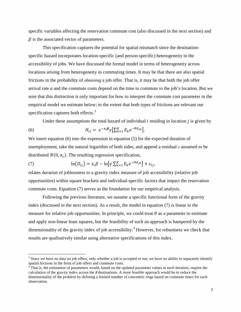
specific variables affecting the reservation commute cost (also discussed in the next section) and

𝛽 is the associated vector of parameters.

This specification captures the potential for spatial mismatch since the destination-

specific hazard incorporates location-specific (and person-specific) heterogeneity in the

accessibility of jobs. We have discussed the formal model in terms of heterogeneity across

locations arising from heterogeneity in commuting times. It may be that there are also spatial

frictions in the probability of obtaining a job offer. That is, it may be that both the job offer

arrival rate a and the commute costs depend on the time to commute to the job’s location. But we

note that this distinction is only important for how to interpret the commute cost parameter in the

empirical model we estimate below; to the extent that both types of frictions are relevant our

specification captures both effects.3

Under these assumptions the total hazard of individual 𝑖 residing in location 𝑗 is given by

(6) 𝐻𝑖𝑗 = 𝑒−𝒙𝑖𝜷𝛾�∑ 𝐸𝑘𝑒−𝜃𝑑𝑗𝑘𝐾𝑘=1 �.

We insert equation (6) into the expression in equation (5) for the expected duration of

unemployment, take the natural logarithm of both sides, and append a residual ε assumed to be

distributed 𝑁(0,𝜎𝜀). The resulting regression specification,

(7) ln�𝐷𝑖𝑗� = 𝑥𝑖𝛽 − ln�𝛾 ∑ 𝐸𝑘𝑒−𝜃𝑑𝑗𝑘𝐾𝑘=1 � + 𝜀𝑖𝑗,

relates duration of joblessness to a gravity index measure of job accessibility (relative job

opportunities) within square brackets and individual-specific factors that impact the reservation

commute costs. Equation (7) serves as the foundation for our empirical analysis.

Following the previous literature, we assume a specific functional form of the gravity

index (discussed in the next section). As a result, the model in equation (7) is linear in the

measure for relative job opportunities. In principle, we could treat 𝜃 as a parameter to estimate

and apply non-linear least squares, but the feasibility of such an approach is hampered by the

dimensionality of the gravity index of job accessibility.4 However, for robustness we check that

results are qualitatively similar using alternative specifications of this index.

3 Since we have no data on job offers, only whether a job is accepted or not, we have no ability to separately identify spatial frictions in the form of job offers and commute costs. 4 That is, the estimation of parameters would, based on the updated parameter values in each iteration, require the calculation of the gravity index across the 𝐾destinations. A more feasible approach would be to reduce the dimensionality of the problem by defining a limited number of concentric rings based on commute times for each observation.

7

A feature of our data is censoring of the dependent variable. In particular, the actual

duration of joblessness (measured in quarters) is only observed if the displaced worker has found

a job within 2 years, or 9 quarters of joblessness (including the quarter of job separation). A

significant fraction (over 20 percent) of the displaced workers in our sample have no reported

earnings within these first 2 years after separation. Thus, the observed duration of joblessness,

𝐷�𝑖𝑗 , is related to the latent joblessness according to

(8) 𝐷�𝑖𝑗 = �ln�𝐷𝑖𝑗� if 𝐷𝑖𝑗 ≤ 8 ln (9) if 𝐷𝑖𝑗 > 8

.

The regression model in equation (7) with a fixed transportation cost parameter and censoring of

the dependent variable governed by the process in equation (4) defines a Tobit model. In

comparison, Ordinary Least Squares (OLS) estimates can be expected to be attenuated towards

zero (Green 1980). To account for the impact of censoring we estimate the parameters of the

model by maximum likelihood. We account for upper censoring of search duration by censoring

the Tobit at >8 quarters – as far as we follow the workers. We also account for clustering of same

quarter new jobs, with a duration of zero, by imposing a lower censoring limit.5

A key econometric challenge for research on spatial mismatch is that local job

accessibility also affects the geographical distribution and sorting of populations of job seekers.

In cross-sectional data, this type of reverse causality translates into a positive correlation between

local job accessibility and labor market outcomes and makes it very difficult to disentangle the

exogenous impact of local job accessibility in the job search process. In contrast, we identify the

effect of local job accessibility in the job search process by explicitly attempting to restrict the

population of job searchers to those who did not become job searchers because of the locally

available job opportunities. As discussed above, we identify workers who separated from their

previous employer during a mass layoff event. Estimates of the impact of local job accessibility

on job search-related outcomes for displaced workers should be less subject to reverse causality

induced by local job opportunities also affecting the local pool of job seekers. We follow the

displacement literature by focusing on workers with strong labor force attachment (at least 4

quarters of tenure with the firm before displacement) who experience a displacement. Focusing

5 Because we use quarterly earnings data to measure duration, we assume that a job is obtained midway through a quarter; in practice, we add 0.5 quarters to duration before taking logs.

8

on workers with strong labor force attachment subject to a mass layoff thus yields a group of at-

risk searchers who are plausibly searching for exogenous reasons.

As will become clear below, we also control for a host of other factors. That is, we

control for demographic, household, employment history, and neighborhood characteristics, for

quarter of separation, and for metropolitan area-by-year effects for the metropolitan area of

residence and quarter of separation.6 In our most stringent specification, we also control for

employer fixed effects.

IV. Data and the Measurement of Job Accessibility

In this section, we describe the data sets used in this project, the measurement of job

accessibility, and the construction of an estimation sample of job seekers. We also present

summary statistics and compare job accessibility within and across populations.

A. Data sources

The technical advances in this study are made possible by the richness of the

Longitudinal Employer-Household Dynamics (LEHD) infrastructure files. The LEHD program

at the Census Bureau constructs the infrastructure files from integrated administrative and survey

data and releases public use data products (see Abowd et al. 2009).7 The data frame provides

virtually universal coverage of workers covered by unemployment insurance. In recent reporting

periods, the LEHD data infrastructure tracks on a quarterly basis more than 140 million jobs held

by over 120 million unique workers at more than 6 million employers. The LEHD infrastructure

files provide precise address information for most employers and workers, which have been

geocoded to Census geographic units. We use the place of residence information to assign

measures of job accessibility to workers at the time of a job loss, which we observe as the

termination of earnings to a worker from an employer. Lastly, we identify if and when a

separated worker obtains a new job.

6 We include metropolitan area by year fixed effects in our specification, but cannot report them because of agreements with the states which supplied the employee data. 7 At the core of the LEHD dataset are two administrative records files provided by state partners to the Census Bureau on a quarterly basis: (1) unemployment insurance wage records, giving the earnings of each worker at each employer, and (2) employer reports giving establishment-level data, known as the Quarterly Census of Employment and Wages (QCEW). Public use datasets derived from the LEHD include the Quarterly Workforce Indicators and the LEHD Origin-Destination Employment Statistics (LODES), available through the web application OnTheMap. The microdata in the LEHD data infrastructure are confidential and protected by U.S.C. Titles 13 and 26. External researchers may access the LEHD dataset for approved statistical purposes at one of the Census Bureau’s Research Data Centers. See <http://www.census.gov/ces> for information on the application process.

9

In addition to extracting the sample of job seekers from the LEHD infrastructure files, we

use the LEHD data to measure the spatial distribution of employment and competing workers.

From the infrastructure files, we aggregate LEHD jobs data to workplace and residence census

tracts.8 We limit the extract to primary, or highest earning, jobs of a worker, and to private sector

jobs only. In order to make the jobs data most relevant to the sample of lower-earning job

searchers, we only consider jobs with annualized earnings of less than $40,000.

This study uses morning, peak-period travel time to provide a better approximation than

straight-line distance of the cost of traveling to a job opportunity from a place of residence.

Metropolitan Planning Organizations (MPOs) estimate both automobile and public transit travel

times between all points in an urban area in order to assess transportation needs, and they have

provided their estimates to us for research purposes. Their modeling incorporates traffic

congestion, so the data approximates “rush hour” conditions where commutes may be slower.

(See Appendix A for more detail on the travel time data.9)

Lastly, we incorporate several neighborhood characteristics available from tabulated data

from the 2000 Census. In particular, we use (long form sample-based) census tract measures of

poverty, home ownership, population density, building vintage, and use of public transit. We

include these variables in estimation models to control for neighborhood characteristics other

than relative job accessibility that may also be related to employment outcomes.

B. Sample Construction

We construct a sample of lower-income job seekers who resided in nine large “Great

Lakes” metropolitan areas. The metropolitan areas we use are those that include the following

cities (listed from west to east): Minneapolis-St. Paul MN, Milwaukee WI, Chicago IL,

Indianapolis IN, Detroit MI, Columbus OH, Cleveland OH, Pittsburgh PA, and Buffalo NY.10 A

major undertaking was to obtain and integrate the MPO data for all of these metro areas into our

8 Our aggregation has a similar structure and degree of geographic detail as the LODES data. 9 To evaluate the quality of this data, we compared the MPO data with morning travel times reported in the 2000 Decennial Census “long form,” made available as public tabulations in the Census Transportation Planning Package (see Table A1). We find that for the set of commute routes available in the CTPP data, automobile travel times are very similar between the two sources. Transit travel times provided by MPOs are somewhat longer than for comparable commutes reported in the CTPP. A crucial advantage of the MPO data over the CTPP is that the MPOs provide a complete matrix of commute times, rather than just those that are actually travelled by the 1-in-6 sample of households responding to the long form. For calculating proximity to potential jobs, we need to know all commute times even if those trips are unlikely. 10 The sets of counties do not correspond exactly with Consolidated Metropolitan Statistical Areas (CMSAs). For example, the Chicago-Naperville-Joliet CMSA includes counties in Illinois, as well as Wisconsin and Indiana. We only use counties with MPO travel time data, which are all in the same state as the principal city.

10

data infrastructure. An advantage of restricting our attention to these areas is that they are in the

same broad region of the U.S. (the Great Lakes) and as such are broadly comparable in many

ways. All nine metropolitan areas have over one million inhabitants and have a broadly similar

spatial configuration of commercial, industrial, and housing location and vintage. They generally

also have clearly discernible central business districts along with substantial suburbanization

over the past 60 years. Although the amount of public transit varies, it usually consists of bus

and/or light rail, and some have heavy rail (e.g., subways). Since early studies and later work on

spatial mismatch focused on cities in this region, using a similar set of cities will facilitate

comparisons to earlier findings. We focus on job searches originating from separations.

Table 1 presents the restrictions used to arrive at our estimation sample, with rounded

sample sizes. We start by extracting a set of almost 10 million workers employed in the states

including our metropolitan areas, and who separated between 2000 and 2005.11 In the LEHD

Employment History File, jobs are identified as an earnings spell for a unique person identifier

from an employer, known by its State Employer Identification Number (SEIN). We identify a

job separation as a termination of earnings where the worker does not resume earning at that

employer for at least 2 full years (and, for cases of multiple simultaneous separations, we retain

only the highest earning separation record). We require that a worker have at least 4 quarters of

tenure prior to the separation to demonstrate attachment both to that employer and to a

residential location that may have been set in relation to the job.

We determine residency within the nine metropolitan areas by linking worker records to

the Composite Person Record (CPR), an annual database produced from federal administrative

data at the Census Bureau providing residential locations for individuals, which can be linked to

LEHD workers using personal identifying information. Because job loss could occur at any point

in a year, and we do not know to which month the CPR address refers, we use place of residence

in the year prior to job loss. Thus, the place of residence of the workers in our sample is not

conditional on job separation, avoiding any concern that a worker relocated as a result of the

separation. Because this study requires neighborhood-level measures of job accessibility, we

only retain workers with a place of residence precise to the census tract level and drop a further

11.6 percent of jobs.

11 Our data are reasonably contemporaneous. Beyond the earnings records, we use demographic and neighborhood information from the 2000 Decennial Census and MPO travel times from the 2000s.

11

We link the sample of separated workers to the “Hundred Percent Edited Detail File”

(HEDF), which provides short form responses to the 2000 Decennial Census. We are able to link

over 85 percent of the remaining separated workers sample to the HEDF, which provides

demographic and household information. We then limit the worker sample to those aged 20 to 64

at the time of job loss.

We apply further restrictions to establish labor market attachment. We calculate LEHD

earnings of the worker over the previous year (from all jobs), and only retain workers with total

earnings between $15,000 and $40,000, about 35 percent of the job loss sample. The lower limit

requires that the worker is working in at least a full-time, minimum wage job. The upper bound

focuses the analysis on lower-earning workers, who have been the principal focus of spatial

mismatch research and who are likely to be more sensitive to local differences in job

accessibility than higher earning workers.12 We also require that the lost job accounted for at

least half of previous year total earnings, and that the job can be linked to the LEHD Employer

Characteristics File, which provides industry, size, and location information for the employer

SEIN.

Lastly, we retain only jobs that can be defined as resulting from a “mass layoff event.”

We use employer-reported workforce size from the Employer Characteristics File to identify

employers that lost over 30 percent of their workforce over a year, with at least 25 workers at the

start of the year. Almost two-thirds of separations occur during such an episode. However, some

of these declines could be specious. A restructuring business might retain its employees but

report the earnings using a new SEIN. Using rules employed in processing of the LEHD

infrastructure files for identifying restructuring, we rule out 59.6 percent of the separations.13

The remainder we classify as separations due to a mass layoff event. Note that the sample of job

separators also excludes any worker who returns to the same employer within 2 years, such as

through a recall, which underscores the involuntary nature of the displacement. While the

resulting sample of approximately 247,000 job seekers formerly at medium-sized and large firms

is much reduced from the original set of separators, we consider these sample reductions as

12 According to Raven et al. (2011) workers with a college education have almost double the interstate migration rate as those with high school or less education. High earning workers also migrate marginally more. 13 The LEHD program compiles a Successor-Predecessor File to document transitions across SEINs for a set of workers (Benedetto et al. 2007).

12

necessary to meet the identification standards to obtain an unbiased estimate of the effect of job

accessibility on unemployment duration.

C. Job Opportunities, Competing Searchers, and Job Accessibility

We measure each job seeker’s job accessibility at the time of his or her separation using a

proximity-weighted index of nearby job opportunities and competing searchers for those jobs.

Worker i, residing in tract j, in year t, may commute by mode m (automobile or transit) to any

tract k in metro area M, indexed from 1 to KM. We define effective job opportunities, 𝐽𝑂𝑖𝑗𝑡𝑚, as

the sum of jobs in all tracts discounted by an impedance function based on a mode’s travel time

to each tract. We use a composite job opportunities measure weighted by the probability of a job

seeker using automobile or transit to reach each tract, calculated as:

(9) 𝐽𝑂𝑖𝑗𝑡𝑚� = ���̂�𝑖𝑗𝑘𝑚𝐸𝑘𝑡

exp �𝜃 ∙ max�0,𝑑𝑗𝑘𝑚 − 𝜏��𝑚

𝐾𝑀

𝑘=1

= �𝐽𝑂𝑖𝑗𝑡𝑘𝑚�

𝐾𝑀

𝑘=1

where m=𝑚� signifies the use of predicted commute mode. The predicted probability of worker i

using either mode, m, to reach tract k is �̂�𝑖𝑗𝑘𝑚, with ∑ �̂�𝑖𝑗𝑘𝑚 = 1𝑚 . In a case where only

automobile travel is an option, job opportunities would simply reduce to a function of auto travel

time, which would be written 𝐽𝑂𝑖𝑗𝑡(auto). We describe the mode choice model in subsection D.

We consider total employment in each census tract, Ek, to be a proxy for the number of

job offers available at that location in year t. As is discussed above, we use the count of LEHD

primary jobs on April 1 of each year as our measure of total employment.14 We use an

impedance function in the denominator of (9) to discount employment more as travel time (d)

from i’s home increases. For this analysis, we use a discounting formula that imposes no

discount for the first 10 minutes of travel. Thus for these short commutes, where djkm ≤ τ, the

denominator of equation (9) equals one and there is no discount. For commutes beyond the travel

time threshold, we use an exponential function of the product of a factor 𝜃 and the surplus travel

14 Examining the Quarterly Workforce Indicators at the county level, we find that the quantity of new hires has a correlation of 0.986 with the stock of beginning-of-quarter jobs. It is reasonable to think about using net job creation to measure job opportunities. However, net job creation only has a correlation of 0.535 with new hires. Shen (2000) also finds that the great majority of job openings occur in locations with an abundance of jobs. Furthermore, competing job seekers is more comparable to job opportunities when the latter is measured as all jobs rather than new hires, since we do not know how many currently employed individuals are true job seekers.

13

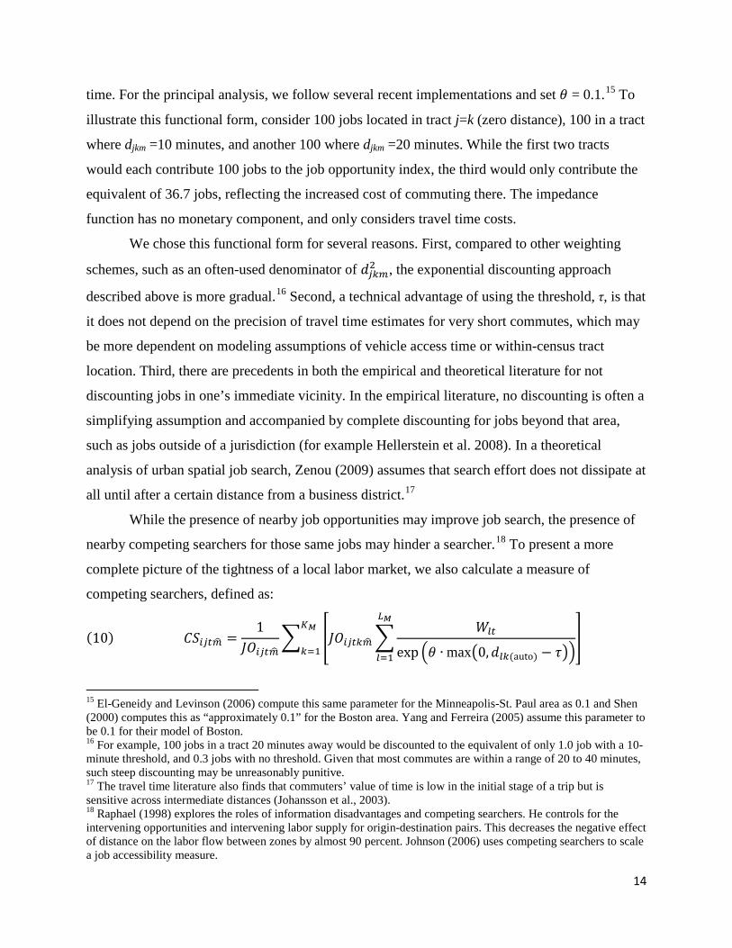
time. For the principal analysis, we follow several recent implementations and set 𝜃 = 0.1.15 To

illustrate this functional form, consider 100 jobs located in tract j=k (zero distance), 100 in a tract

where djkm =10 minutes, and another 100 where djkm =20 minutes. While the first two tracts

would each contribute 100 jobs to the job opportunity index, the third would only contribute the

equivalent of 36.7 jobs, reflecting the increased cost of commuting there. The impedance

function has no monetary component, and only considers travel time costs.

We chose this functional form for several reasons. First, compared to other weighting

schemes, such as an often-used denominator of 𝑑𝑗𝑘𝑚2 , the exponential discounting approach

described above is more gradual.16 Second, a technical advantage of using the threshold, τ, is that

it does not depend on the precision of travel time estimates for very short commutes, which may

be more dependent on modeling assumptions of vehicle access time or within-census tract

location. Third, there are precedents in both the empirical and theoretical literature for not

discounting jobs in one’s immediate vicinity. In the empirical literature, no discounting is often a

simplifying assumption and accompanied by complete discounting for jobs beyond that area,

such as jobs outside of a jurisdiction (for example Hellerstein et al. 2008). In a theoretical

analysis of urban spatial job search, Zenou (2009) assumes that search effort does not dissipate at

all until after a certain distance from a business district.17

While the presence of nearby job opportunities may improve job search, the presence of

nearby competing searchers for those same jobs may hinder a searcher.18 To present a more

complete picture of the tightness of a local labor market, we also calculate a measure of

competing searchers, defined as:

(10) 𝐶𝑆𝑖𝑗𝑡𝑚� =1

𝐽𝑂𝑖𝑗𝑡𝑚�� �𝐽𝑂𝑖𝑗𝑡𝑘𝑚� �

𝑊𝑙𝑡

exp �𝜃 ∙ max�0,𝑑𝑙𝑘(auto) − 𝜏��

𝐿𝑀

𝑙=1

�𝐾𝑀

𝑘=1

15 El-Geneidy and Levinson (2006) compute this same parameter for the Minneapolis-St. Paul area as 0.1 and Shen (2000) computes this as “approximately 0.1” for the Boston area. Yang and Ferreira (2005) assume this parameter to be 0.1 for their model of Boston. 16 For example, 100 jobs in a tract 20 minutes away would be discounted to the equivalent of only 1.0 job with a 10-minute threshold, and 0.3 jobs with no threshold. Given that most commutes are within a range of 20 to 40 minutes, such steep discounting may be unreasonably punitive. 17 The travel time literature also finds that commuters’ value of time is low in the initial stage of a trip but is sensitive across intermediate distances (Johansson et al., 2003). 18 Raphael (1998) explores the roles of information disadvantages and competing searchers. He controls for the intervening opportunities and intervening labor supply for origin-destination pairs. This decreases the negative effect of distance on the labor flow between zones by almost 90 percent. Johnson (2006) uses competing searchers to scale a job accessibility measure.

14

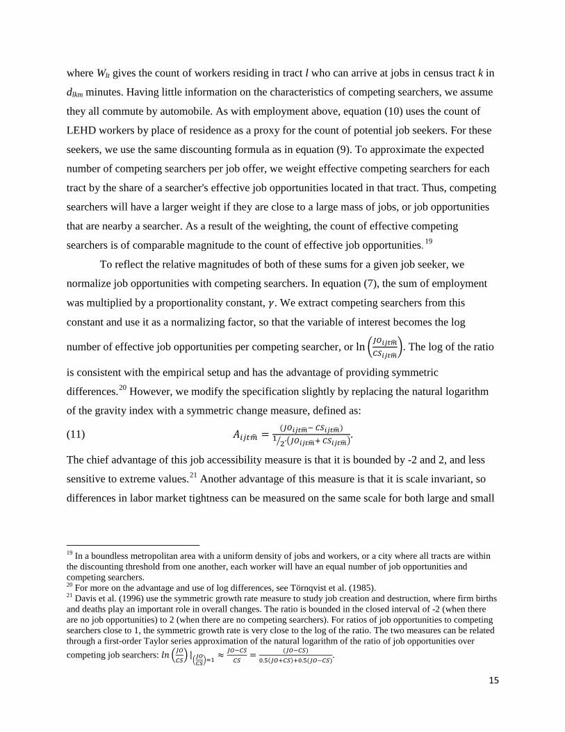
where Wlt gives the count of workers residing in tract l who can arrive at jobs in census tract k in

dlkm minutes. Having little information on the characteristics of competing searchers, we assume

they all commute by automobile. As with employment above, equation (10) uses the count of

LEHD workers by place of residence as a proxy for the count of potential job seekers. For these

seekers, we use the same discounting formula as in equation (9). To approximate the expected

number of competing searchers per job offer, we weight effective competing searchers for each

tract by the share of a searcher's effective job opportunities located in that tract. Thus, competing

searchers will have a larger weight if they are close to a large mass of jobs, or job opportunities

that are nearby a searcher. As a result of the weighting, the count of effective competing

searchers is of comparable magnitude to the count of effective job opportunities.19

To reflect the relative magnitudes of both of these sums for a given job seeker, we

normalize job opportunities with competing searchers. In equation (7), the sum of employment

was multiplied by a proportionality constant, 𝛾. We extract competing searchers from this

constant and use it as a normalizing factor, so that the variable of interest becomes the log

number of effective job opportunities per competing searcher, or ln �𝐽𝑂𝑖𝑗𝑡𝑚�𝐶𝑆𝑖𝑗𝑡𝑚�

�. The log of the ratio

is consistent with the empirical setup and has the advantage of providing symmetric

differences.20 However, we modify the specification slightly by replacing the natural logarithm

of the gravity index with a symmetric change measure, defined as:

(11) 𝐴𝑖𝑗𝑡𝑚� =(𝐽𝑂𝑖𝑗𝑡𝑚�− 𝐶𝑆𝑖𝑗𝑡𝑚�)

12� ∙�𝐽𝑂𝑖𝑗𝑡𝑚�+ 𝐶𝑆𝑖𝑗𝑡𝑚��

.

The chief advantage of this job accessibility measure is that it is bounded by -2 and 2, and less

sensitive to extreme values.21 Another advantage of this measure is that it is scale invariant, so

differences in labor market tightness can be measured on the same scale for both large and small

19 In a boundless metropolitan area with a uniform density of jobs and workers, or a city where all tracts are within the discounting threshold from one another, each worker will have an equal number of job opportunities and competing searchers. 20 For more on the advantage and use of log differences, see Törnqvist et al. (1985). 21 Davis et al. (1996) use the symmetric growth rate measure to study job creation and destruction, where firm births and deaths play an important role in overall changes. The ratio is bounded in the closed interval of -2 (when there are no job opportunities) to 2 (when there are no competing searchers). For ratios of job opportunities to competing searchers close to 1, the symmetric growth rate is very close to the log of the ratio. The two measures can be related through a first-order Taylor series approximation of the natural logarithm of the ratio of job opportunities over

competing job searchers: 𝑙𝑛 �𝐽𝑂𝐶𝑆� |

�𝐽𝑂𝐶𝑆�=1≈ 𝐽𝑂−𝐶𝑆

𝐶𝑆= (𝐽𝑂−𝐶𝑆)

0.5(𝐽𝑂+𝐶𝑆)+0.5(𝐽𝑂−𝐶𝑆).

15

metropolitan areas. Substituting the job accessibility ratio from (11) into the regression

specification in (7), we obtain the estimation model,

(12) 𝐷�𝑖𝑗𝑡 = 𝛼𝐴𝑖𝑗𝑡𝑚� + 𝑥𝑖𝑗𝑡𝛽 + 𝜀𝑖𝑗𝑡.

where 𝛼 is the parameter of interest. In practice, we only retain the first or only observation of

job search for each displaced worker, so there is a direct mapping between i, j, and t.

D. Mode choice prediction

A unique feature of our approach is that we construct person-specific job accessibility

measures taking into account not only the heterogeneity across locations but also person-specific

differences in mode choice, �̂�𝑖𝑗𝑘𝑚. A detailed description of the estimation of the predicted mode

choice probabilities is in Appendix B but we provide a brief description here. We estimate

logistic models for vehicle ownership and mode choice using journey-to-work responses from

the 2000 Decennial Census long form combined with the MPO travel time data, by mode, and

LEHD earnings records. We then use the parameter estimates to make out-of-sample predictions

of vehicle ownership and mode choice probabilities for each possible commute destination for

each person in the displaced worker sample. Because automobile travel is faster on most routes,

that is, 𝑑𝑗𝑘(auto) < 𝑑𝑗𝑘(transit), it is usually true that a car driver can reach more jobs in the same

time (though at greater cost), making 𝐽𝑂𝑖𝑗𝑡𝑘(auto) > 𝐽𝑂𝑖𝑗𝑡𝑘(transit). Thus, a worker with a higher

probability of vehicle ownership and automobile use will tend to have more effective job

opportunities in a given destination, and greater job accessibility overall.22

Estimation results from the vehicle ownership and mode choice model are intuitive (See

Appendix Table B3). For the vehicle ownership model, we find that larger and higher-earning

households, and households in neighborhoods with poor quality transit are more likely to have

vehicles; blacks and households in densely populated areas are less likely to own. For the mode

choice model, we find that lower income workers are more likely to use public transit on a route,

even if there is poor transit access on the route, while higher income workers tend to use transit

only if it is competitive with automobile travel times.

22 Raphael and Stoll (2001) approach spatial mismatch by asking if increasing minority automobile ownership rates can narrow inter-racial employment gaps. Making a comparison across metropolitan areas, they find that having access to a car is particularly important for blacks and Latinos, and that the difference in employment rates between car-owners and non-car-owners that is greater among blacks than among whites. Johnson (2006, p. 361) finds that “access to a car while searching is estimated to increase the weekly hazard of successfully completing a job search by 49.8%.”

16

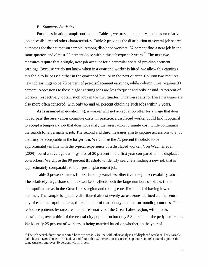
E. Summary Statistics

For the estimation sample outlined in Table 1, we present summary statistics on relative

job accessibility and other characteristics. Table 2 provides the distribution of several job search

outcomes for the estimation sample. Among displaced workers, 32 percent find a new job in the

same quarter, and almost 80 percent do so within the subsequent 2 years.23 The next two

measures require that a single, new job account for a particular share of pre-displacement

earnings. Because we do not know when in a quarter a worker is hired, we allow this earnings

threshold to be passed either in the quarter of hire, or in the next quarter. Column two requires

new job earnings to be 75 percent of pre-displacement earnings, while column three requires 90

percent. Accessions to these higher earning jobs are less frequent and only 22 and 19 percent of

workers, respectively, obtain such jobs in the first quarter. Duration spells for these measures are

also more often censored, with only 65 and 60 percent obtaining such jobs within 2 years.

As is assumed in equation (4), a worker will not accept a job offer for a wage that does

not surpass the reservation commute costs. In practice, a displaced worker could find it optimal

to accept a temporary job that does not satisfy the reservation commute cost, while continuing

the search for a permanent job. The second and third measures aim to capture accessions to a job

that may be acceptable in the longer run. We choose the 75 percent threshold to be

approximately in line with the typical experience of a displaced worker. Von Wachter et al.

(2009) found an average earnings loss of 20 percent in the first year compared to not-displaced

co-workers. We chose the 90 percent threshold to identify searchers finding a new job that is

approximately comparable to their pre-displacement job.

Table 3 presents means for explanatory variables other than the job accessibility ratio.

The relatively large share of black workers reflects both the large numbers of blacks in the

metropolitan areas in the Great Lakes region and their greater likelihood of having lower

incomes. The sample is spatially distributed almost evenly across zones defined as: the central

city of each metropolitan area, the remainder of that county, and the surrounding counties. The

residence patterns by race are also representative of the Great Lakes region, with blacks

constituting over a third of the central city population but only 5.8 percent of the peripheral zone.

We identify 25 percent of workers as being married based on whether, in the year of

23 The job search durations reported here are broadly in line with other analyses of displaced workers. For example, Fallick et al. (2012) used LEHD data and found that 37 percent of distressed separators in 2001 found a job in the same quarter, and over 80 percent within 1 year.

17

displacement, they were still residing with a spouse listed on the 2000 Decennial Census

response. We then attribute LEHD earnings to each spouse to construct household earnings

variables and to classify a person as a primary or secondary earner in the household. We group

workers by displacing employer industry into five broad categories.24 Almost 40 percent of

displacements are from goods-producing industries, and 28 percent of job losses occurred during

and following the 2001 recession. Displacements were evenly spaced throughout the year. Using

the travel time measures and establishment locations from the ECF, we produce indicators of

whether a previous job’s commute was <20, 20 to 40, or >40 minutes drive time, and find a

roughly even distribution across those ranges.25 From the LEHD data, we find that displaced

workers had, on average, well over a year of tenure, and lost a job with annual earnings of

approximately $27,000.26 Neighborhood variables from the 2000 Census show an average

poverty rate of 10.7 percent in their residence census tract, with 7.4 percent of neighbors using

transit.

Figure 1 and Table 4 provide information on the distribution of the job accessibility

variable, using the measure based on predicted travel mode, per equation (11). The normalization

of job opportunities and competing searchers allows us to compare job accessibility levels across

a significant range of (large) metropolitan area sizes, even though the absolute count of jobs and

searchers may vary considerably depending on metropolitan area size. We include no controls,

but explore subsamples to highlight differences in job accessibility. Figure 1 presents the percent

distribution of displaced workers by bins of width 0.25 across the full range of -2 to 2. The

median job accessibility of 0.036 is greater than zero, but the overall distribution skews slightly

higher in the area below zero; that is, on average, competing searchers slightly exceed job

opportunities for jobs earning $15,000-$40,000.

Table 4 provides information on how job accessibility varies by location and across

subsamples. There is considerable spatial variation in our measure of accessibility. The median is

0.339 for workers living in the central city, 0.098 for workers living in the central county (but not

the central city), and -0.285 for workers living outside the central county. This distribution is in

keeping with the spatial structure of large, older Great Lakes metropolitan areas. In most cases,

24 Industries aggregated as follows: Goods-Producing and Distribution (North American Industrial Classification System sectors 11,21,22,23,31-33,42,48,49), Local Services (44,45,56,71,72,81), Professional Services (51,52,53,54,55), Education and Public (61,92), Health Care (62). 25 The national average one-way travel time for U.S. workers was 25.5 minutes in 2000 (McKenzie 2013). 26 Recall that we restricted the sample to workers earning between $15,000 and $40,000.

18

there is a great deal of employment in the central business district and adjoining areas even

though substantial suburbanization of jobs has occurred. In those cases, measures of job

accessibility can be seen as a set of concentric circles with accessibility declining as distance

from the central business district increases. While the exact shape of these circles will vary

according to highway and transit patterns, the general pattern will remain (for an example from a

large, older metropolitan area, see Fisher et al. 2009). Our job accessibility measure, of course,

also includes competing searchers. The number of competing searchers for central city lower-

income jobs exceeds the comparable number in suburban locations. However, as reflected in our

job accessibility index, job opportunities relative to competing searchers are higher in central

areas and lower in suburban areas.27

Given the overall spatial pattern of job accessibility, it is not surprising that our

accessibility index varies across demographic groups due to differing residential location

patterns. While blacks have higher median job accessibility than white non-Hispanics and

Hispanics, this largely reflects their concentrated residence in neighborhoods that are typically

closer to a high-employment central business district; 71 percent of the blacks in our sample

reside in central cities, compared to 36 percent of the full sample. Put differently, while blacks

constitute 19 percent of the full sample, they make up 37 percent of the sample residing in the

central city of each metropolitan area (see Table 3).28 In fact, central city whites actually have

higher job accessibility (0.439) than blacks (0.333). This may reflect whites’ higher likelihood of

commuting by auto. Our use of predicted mode choice lowers the job accessibility measure for

blacks, who are much more likely to be users of public transportation due to their lower rates of

vehicle ownership.

V. Results for Unemployment Duration and Spatial Mismatch

In this section, we empirically test whether the job search model that incorporates the

gravity index of local job accessibility explains the variation in the duration of joblessness

among displaced workers. If estimation of our model provides support for a causal negative link

27 One concern might be that our sample of displaced workers is not representative. In results not presented here, we also calculate the median job accessibility across all Census tracts, using the 2000 Census population and 2000 Census labor force for weights, and find little difference. 28 The finding of higher job accessibility for blacks varies across studies, which vary widely in measures employed and metropolitan areas considered. Hellerstein et al. (2008) finds higher overall job accessibility for blacks, but lower accessibility to lower-education jobs. Note also that many downtown jobs require higher education levels that are not compatible with the $40,000 earnings threshold imposed for this sample.

19

between job accessibility and duration of joblessness, then we will have provided support for the

spatial mismatch hypothesis along with an estimate of the strength of this phenomenon. Table 5

presents the main upper- and lower-censored Tobit estimation result relating job search success

(as measured by the log of quarters of search duration) to the job accessibility ratio and control

variables, as specified in equation (12). We define success as in Table 2 – finding any job (in

column one), finding a job that provides more than 75 percent of earnings at the previous job (in

column two), or finding a job that provides more than 90 percent of earnings at the previous job

(in column three). We calculate job accessibility as in equation (11), using predicted travel times

to weight the contribution of jobs and competing searchers. A negative coefficient signifies that

better access reduces the duration of joblessness.

For each dependent variable specification, we find that greater job accessibility reduces

job search duration, with greater effects for jobs with incomes approaching the earnings of the

lost job. In the center of the distribution, an increase of one unit in job accessibility (from -0.5 to

0.5) is approximately equal to an increase from the 20th to the 80th percentile of job accessibility

(see Figure 1). Such an increase is associated with a 5.0 percent reduction in search duration for

finding any job, and a 6.6 and 8.3 percent reduction for accessions to a new job with 75 and 90

percent of prior job earnings, respectively. The greater effect for the higher earnings thresholds is

consistent with reduced noise in the dependent variable as the “any new job” outcome in column

one includes temporary jobs, that is, a job that a displaced worker would not maintain in the long

term. The results for higher earning jobs may also better reflect the tradeoff of offer value and

commute distance faced by a job seeker. Imposing the threshold is equivalent to reducing the

offer arrival rate given by equation (5), which is expected to increase search duration. Only new

jobs within the same state are included, so long distance relocations resulting in a new job are

considered a failure to find a local job.29

To evaluate the importance of focusing on mass layoff events, we also estimate the

search model for a comparable sample of over 300,000 non-displaced separators (not presented

here). For non-displaced searchers, we can find no statistically significant relationship between

29 All of the metropolitan areas we consider are in a CMSA that is either entirely or mostly contained within one state (the exceptions are 5 of 14 counties in Chicago-Naperville-Joliet IL-IN-WI and 2 of 13 in Minneapolis-St. Paul-Bloomington MN-WI). As is discussed earlier, the MPOs used to define residence counties are only in the state of the principal city.

20

job accessibility and search duration. This finding highlights the importance of focusing on

persons who are searching for plausibly exogenous reasons.

The specifications presented in Table 5 include controls for demographic characteristics,

for previous employer’s industry, for each metropolitan area by year, and for the quarter of job

loss. The total impact of the controls signifies the importance of controlling for other factors

related to selection of a residence location. Although it is not always possible to determine a

prior expectation, none of the coefficients associated with the control variables have signs that

are unusual, and the effects are highly significant, suggesting that the model is well-specified and

that the controls are helping with identification. The directions and magnitudes of the control

variables vary little across specifications. Men, white non-Hispanics, and younger workers tend

to have shorter search duration. Workers with greater lost earnings find jobs faster, but those

with greater annual earnings or annual household earnings take more time, corresponding to a

higher reservation wage or a greater financial cushion. Workers having held many jobs in the last

2 years find a new job faster, as do those who commuted farther to a previous job, suggesting a

lower reservation commute cost. Residents of high poverty tracts take longer to find a job while

those in high homeownership and more recently developed tracts find a job faster. Workers

previously employed in goods-producing industries, including manufacturing, and those in

education or public services, take longer to find a new job.

Although not shown here, the control variables are helpful in identifying the main effect.

Dropping the neighborhood variables reduces the main effect by one-half, and dropping the

employment history variables reduces it by one-half again. As is discussed in Appendix C, this

primary result of reduced search duration associated with increased job accessibility is robust to

variation in the specification of the gravity index and choice of outcome variable. We find

similar results employing other statistical models (such as the ordered logit, and variations in

censoring.

Table 6 presents the main estimate from Table 5, along with other estimates to evaluate

the robustness of this result to employer selection. As discussed above, one concern is that the

unobserved ability of a job seeker may be related to job search outcomes and place of residence.

To control for a potential indicator of ability, we estimate a specification with fixed effects for

the previous employer, which controls for sorting to employers with respect to unobserved

characteristics. The linear non-censored specification shown in column three includes 31,000

21

fixed effects for workers sharing an employer; other control variables remain the same, but

industry and metropolitan area effects fall out. We again find a significant negative effect of job

accessibility in column three for both the 75 percent and 90 percent of previous job earnings

outcomes (the “any new job” outcome also has a negative but not a significant coefficient). To

compare the magnitude of this effect with the result in column one, we also estimate a non-

censored model using OLS, with no employer effects (column two). Based on what has been

observed to be a powerful empirical regularity (Green 1980), we can rescale the OLS result by

dividing the estimated coefficient by the share that is not censored in the Tobit regression (42.7

percent for the 75 percent earnings threshold). For each outcome, the rescaled OLS coefficient in

column four is similar in magnitude to the censored Tobit estimate in column one. Finally, we

rescale the fixed effects estimate using the same factor, providing the estimate in column five.

The rescaled fixed effects estimates for the 75-percent and 90-percent earnings thresholds are

approximately half the magnitude of the primary result.

One drawback of the fixed effects model is that, because many workers reside relatively

nearby to where they work, the degree of variation in job accessibility among co-workers will be

substantially less than among the full population. We conclude that the robustness of the main

result to employer fixed effects underscores our spatial mismatch finding, but we focus on the

Tobit model without employer effects for other extensions and interpretation.

Table 7 presents the distribution of expected search durations given job accessibility at

the median (with a value of 0.036), and the expected change in durations associated with a jump

from the 25th to the 75th percentile of job accessibility (values of -0.403 and 0.438 respectively).

As with Table 2, expected search duration rises with the earnings threshold. Job seekers with

median accessibility are expected to find any new job (column 1), or a job with the 75 and 90

percent earnings thresholds (columns 3 and 5) in the same quarter with a probability of 0.41,

0.29, and 0.25 respectively.30 Around these medians, the 75-25 difference columns show that

substantially greater job accessibly would improve same quarter job finding by about 1

percentage point (0.74, 0.78, and 0.89 percentage points, respectively).

30 The expected probabilities from the Tobit model are skewed towards earlier new jobs compared with the population averages in Table 2. The expectations at mean job accessibility are very similar to those at the 50th percentile. The difference of Tables 6 and 2 is likely due to the linear functional form imposed by the Tobit model. For an ordered logit model, where the number of search quarters is the dependent variable, expectations are closely in line with the population averages.

22

Overall, the Table 5 results imply that an increase from the 25th to the 75th percentile of

job accessibility is associated with a 4.2 percent reduction in search duration for finding any job,

and a 5.6 and 7.0 percent reduction for accessions to a new job with 75 and 90 percent of prior

job earnings, respectively. The greater magnitude of the high earning outcome reflects the higher

sensitivity of obtaining such a job to spatial mismatch.

The magnitude of our estimated effect of job accessibility can be put into perspective by

comparing it against the effect of other neighborhood characteristics. For example, the 25th and

75th percentiles of the census tract poverty rate for our sample are 0.037 and 0.142 (with a mean

of 0.106 and a median of 0.070). In Table 5, we find a positive effect on job search duration for

neighborhood poverty, so moving from a high to low poverty neighborhood, a decrease of

0.105, would be expected to reduce job search time by 1.5, 4.6, and 6.4 percent respectively for

the three job search outcomes. While demographic and job history factors still play the principal

role in determining job search outcomes (blacks take 24 percent longer to find a comparable job),

the similarity in magnitudes of these census tract effects suggests that job accessibility is an

important metric for characterizing a neighborhood. Job accessibility captures a different

dimension of a neighborhood than is represented by tabulations of resident data, with a

correlation of only 0.15 with poverty share (conditional on metropolitan area), and similarly low

relationships with other neighborhood variables.

Table 8 presents results for various subsamples, with the job accessibility estimate from

an independent regression in each cell. As with the main results, estimates for the effect on

finding any job tend to be less significant and more attenuated, while estimates for earnings

greater than 90 percent of previous job estimates are strongest. These subsample results highlight

some groups that are especially sensitive to spatial mismatch, but also suggest that job

accessibility is broadly relevant for all job seekers. Larger magnitude effects may reflect both

greater sensitivity to job accessibility or differences in the suitability of the job accessibility

measure across groups. We cannot be certain of the explanation for any particular group, but

offer some interpretation below.

Panel A of Table 8 shows results disaggregated by race and ethnicity, a reference point of

particular interest for the spatial mismatch literature, which has often focused on outcomes for

lower-earnings inner-city blacks. We first note that non-Hispanic whites, non-Hispanic blacks,

and Hispanics are all sensitive to job accessibility. However, we do find that for obtaining

23

comparable jobs, blacks are especially sensitive evaluated at the point estimates. For finding any

job, a job at 75 percent of previous earnings, or a job at 90 percent of previous earnings, blacks

are more sensitive to job accessibility than whites. Table 8 shows that the relative white-black

coefficients for these three cases are -0.042 versus -0.072, -0.072 versus -0.083, and -0.086

versus -0.116, signifying that blacks are approximately 71, 15, and 35 percent more sensitive

than whites for the three earnings levels examined (although the differences are not statistically

different from each other). We also note that Hispanic job seekers are most sensitive for finding

any job. This could possibly be due to Hispanics being more likely to take a lower earning job

that is accessible rather than holding out for a higher earning job (that is, they have a lower

reservation wage). Put in terms of Table 7, an increase from the overall 25th to 75th percentiles of

job accessibility would be expected to increase a white, black, and Hispanic job seeker's

probability of finding a comparable new job at 75 percent of previous earnings in the first two

quarters by 0.94, 1.10, and 0.98 percentage points respectively, around outcomes of 41.7, 36.6,

and 36.6 percent at median job accessibility for the three groups.

Panel B of Table 8 shows results by sex and age. While men and women have little

difference in outcomes for finding any job, women are especially sensitive to job accessibility

for finding a comparable job, with an effect that is 71 percent greater than that for men. This

result may suggest that men are more likely to accept a long commute to retain lost earnings.

Workers aged 55 to 64 are substantially more sensitive to job accessibility for all earnings

outcomes, with the effect on obtaining a comparable job being almost three times greater than for

those aged 34 to 54. Again, this would suggest that younger workers might be more willing to

commute, or perhaps to relocate locally in order to obtain a new job. A 25th the 75th percentile

change in job accessibility for a female or older job seeker would be expected to reduce search

times for a job earning 75 percent of their previous job by 6.9 and 15.1 percent respectively.

Panel C shows differences by household type and earnings level. Among married

households, there is suggestive evidence that secondary workers, or the lesser earner in a

household, may be more sensitive to spatial mismatch. This sensitivity would be consistent with

a higher reservation wage or a comparative advantage in household production. Not-married

workers, or those for whom we could not establish spousal co-residence, also appear to have

more sensitivity. Workers with greater pre-displacement earnings (those earning $30,000-

$39,999) are actually more sensitive than lower-earning workers ($15,000-$29,999). Again, this

24

result would suggest that spatial mismatch is not just a concern in regards to those with very low

incomes, but is relevant to search outcomes for workers at somewhat higher incomes as well.31

In Panel D, we find that all displaced industry groups are sensitive to job accessibility,

especially when search outcomes are defined as a comparable job. Those displaced from typical

blue-collar industries, labeled here as “goods-producing” (including construction, manufacturing,

utilities, and distribution), are especially sensitive to spatial mismatch. Workers displaced from

public sector and education jobs are also highly sensitive. Health care workers have a similar

accessibility effect across all outcome types, suggesting that such workers are primarily finding

new jobs with similar earnings to their previous jobs. The lower magnitude effect for local

services workers may simply reflect a greater accumulation of job search experience by workers

in a high turnover industry. Alternately, given that the job opportunities in local services are

more spatially distributed, job accessibility may be less of a constraint.

In Table 9, we provide estimates for the effect of job accessibility in the same

race/ethnicity or industry as the job searcher as a means to further refine the set of job

opportunities and competing searchers that might be most relevant. Racial mismatch may be

important (see Hellerstein et al. 2008), which would make race/ethnicity-based accessibility

measures more relevant than the overall measures. Similarly, skills specific to industries might

make industry-based measures more relevant. While our analysis on these dimensions is only

exploratory, the results in Table 9 show that the same-type results for race-ethnicity and industry

are largely similar to the overall job accessibility effects. 32 In short, we do not find evidence that

the impact of spatial mismatch is greater if we refine the accessibility measures to same-type

measures on these dimensions. If anything, we find somewhat weaker results for blacks when

using same-type measures. Part of the reason for these findings is that there is a high degree of

correlation between accessibility for all jobs, and same race/ethnicity jobs, with a correlation of

31 One should not necessarily infer that even higher earning workers would be yet more sensitive, as responsiveness to job accessibility with respect to earnings or skill levels may be non-linear. 32 One difference for the industry results is that those laid off from the public and education sectors are not especially sensitive to opportunities in those industries. One reason for this attenuation may be that we exclude state and local government jobs from our job accessibility measure, because such jobs are often measured with less geographic precision (for example, local school jobs are sometimes reported in one central administrative location rather than distributed to worksites).

25

0.99 for whites, and 0.92 for blacks (conditional on metropolitan area).33 Likewise, we find

similarly high correlations of all and same-sector jobs.

VI. Conclusions

The spatial mismatch hypothesis (SMH) encompasses a wide range of research questions,

all focused on whether a worker with locally inferior access to jobs is likely to have worse labor

market outcomes. The literature grew out of two papers by Kain (1964, 1968), which proposed

that persistent unemployment in urban black communities might be due to a movement of jobs

away from those areas, coupled with the inability due to housing discrimination for those

residents to relocate closer to jobs. A voluminous literature has ensued in an attempt to address

the existence and extent of spatial mismatch. A primary concern has been how to state the

problem and appropriately test for it.

Numerous contributions have advanced this literature, including, for example, explicit

recognition of the value of automobile availability for search and commuting, use in some cases

of commute times instead of distance, and consideration of competing searchers. But no study

has combined and built upon these advances, using appropriate data and satisfactorily dealing

with identification. Furthermore, the existing literature has been primarily cross-sectional, and

despite efforts to account for endogenous residential location, has come under considerable

criticism. More recent efforts at longitudinal analysis by Dawkins et al. (2005), Johnson (2006),

and Rogers (1997) find evidence of spatial mismatch but have smaller samples and identification

challenges.

Relative to this existing longitudinal literature, the analysis in this paper is the first to

focus on workers displaced from a mass layoff, which is a critical aspect of our identification

strategy. The basis of our approach is that if spatial mismatch is present, then the duration of

search for a new job after a displacement event should be related to accessibility to appropriate

jobs. In this paper, we provide a new approach to the measurement of the effects of spatial

mismatch that combines methodological innovation with unique longitudinal and cross-sectional

data for nine, major US metropolitan areas. We take advantage of rich, matched employer-

33 These high correlations persist even when the impedance function in equations (9) and (10) uses a shorter discounting threshold of 5 minutes, rather than the default of 10 minutes. This might have been relevant as Hellerstein et al. (2008) focus on job accessibility measures based on jobs in adjacent zip codes to the place of residence.

26

employee administrative data on job histories and search outcomes integrated with worker

characteristics and neighborhood data from the Decennial Census and comprehensive

transportation network data from nine large Great Lakes metropolitan areas. In addition, our

study casts a much wider geographic net to include suburbs and multiple large metropolitan

areas.

In summary, the key methodological advances we incorporate are (1) deriving a space-

dependent theoretical model consistent with the job search literature; (2) linking data from

several sources to create a large and rich dataset as the basis for estimation, allowing for controls

at the census tract level across nine metropolitan areas and six years; (3) employing a

longitudinal worker history for lower-paid workers with strong labor force attachment to control

for unobservable characteristics of potential workers that may be correlated with residential

location; (4) following a large sample of involuntarily displaced workers, which permits treating

their residential location as exogenously determined; (5) creating an individual-specific job

accessibility measure that accounts for job opportunities, competing searchers, and modal choice

(automobile versus public transit); and (6) using a censored Tobit model to account for censoring

in the dependent variable (unemployment duration).

Our results support the spatial mismatch hypothesis. We find that better job accessibility

significantly decreases the duration of joblessness among lower-paid displaced workers. In the

center of the job accessibility distribution, an increase from the 25th to the 75th percentile of job

accessibility is associated with a 4.2 percent reduction in search duration for finding any job, and

a 5.6 and 7.0 percent reduction for accessions to a new job with 75 and 90 percent of prior job

earnings, respectively. While job accessibility is only one of many factors affecting job search

outcomes, it appears to play an especially important role for blacks, who have long been a focus

of this research area. We find that blacks are approximately 71, 15, and 35 percent more

sensitive to job accessibility than white job seekers for these three hiring measure respectively.

We also find that job accessibility is especially important for females and older workers.

27

REFERENCES Abowd, John M., Bryce Stephens, Lars Vilhuber, Fredrik Andersson, Kevin McKinney, Marc

Roemer, and Simon Woodcock. 2009. “The LEHD Infrastructure Files and the Creation of the Quarterly Workforce Indicators.” In Timothy Dunne, J. Bradford Jensen and Mark J. Roberts, (Eds.) Producer Dynamics: New Evidence from Micro Data. Chicago: University of Chicago Press for the National Bureau of Economic Research, pp. 149-230.

Baum, Charles L. 2009. “The Effects of Vehicle Ownership on Employment.” Journal of Urban

Economics 66, pp. 151-163.

Bellman, Richard E. 1957. Dynamic Programming. Princeton, NJ: Princeton University Press. Benedetto, Gary, John Haltiwanger, Julia Lane, and Kevin McKinney. 2007. “Using Worker

Flows to Measure Firm Dynamics,” Journal of Business and Economic Statistics, 25:3, pp. 299-313.

Bhat, Chandra, Susan Handy, Kara Kockelman, Hani Mahmassani, with Qinglin Chen and Lisa

Weston. 2000. “Measurement of an Urban Accessibility Index: Literature Review.” The University of Texas at Austin Center for Transportation Research, Research Report Number 4938-1 to the Texas Department of Transportation, May.

Brueckner, Jan K. and Yves Zenou. 2003. “Space and Unemployment: the Labor-Market Effects of Spatial Mismatch.” Journal of Labor Economics 21:1, pp. 242-266.

Bunel, Mathieu and Elisabeth Tovar. 2013. “Key Issues in Local Job Accessibility Measurement:

Different Models Mean Different Results.” Urban Studies, pp. 1-17. Dawkins, Casey, Qing Shen, and Thomas Sanchez. 2005. “Race, space, and unemployment

duration.” Journal of Urban Economics 58, pp. 91–113. Davis, Steven, John Haltiwanger, and Jason Faberman. 2012. “Labor Market Flows in the Cross

Section and Over Time.” Journal of Monetary Economics 59:1, pp. 1-18. Davis, Steven, John Haltiwanger, and Scott Schuh. 1996. Job Creation and Destruction.

Cambridge: MIT Press. El-Geneidy, Ahmed M., and David M. Levinson. 2006. “Access to Destinations: Development of

Accessibility Measures.” University of Minnesota Networks, Economics, and Urban Systems Research Group, Final Report to the Minnesota Department of Transportation, May.

Fallick, Bruce, John Haltiwanger, and Erika McEntarfer. 2012. “Job-to-Job Flows and the

Consequences of Job Separations.” Finance and Economics Discussion Series (FEDS) No. 2012-73.

28

Fisher, Lynn, Henry Pollakowski, and Jeffrey Zabel. 2009. “An Amenity-Based Housing Affordability Index,” Real Estate Economics 37:4, pp. 705-746.

Glaeser, Edward L. 1996. “Discussion of O'Regan and Quigley’s ‘Spatial Effects upon

Employment Outcomes’.” New England Economic Review (May/June) pp. 58-64. Gobillon, Laurent, Harris Selod, and Yves Zenou. 2007. “The Mechanisms of Spatial

Mismatch.” Urban Studies 44:12, pp. 2401–2427. Gobillon, Laurent, Thierry Magnac, and Harris Selod. 2011. “The Effect of Location on Finding

a Job in the Paris Region.” Journal of Applied Econometrics 26, pp 1079-1112. Green, W. (1980): “On the Asymptotic Bias of the Ordinary Least Squares Estimator of the

Tobit Model,” Econometrica 48, pp. 27-56.

Handy, Susan L. and Deb A. Niemeier. 1997. “Measuring Accessibility: An Exploration of Issues and Alternatives.” Environment and Planning A 29, pp. 1175-1194.

Hellerstein, Judith K., David Neumark, and Melissa McInerney. 2008. “Spatial Mismatch or Racial Mismatch?” Journal of Urban Economics 64, pp. 464-479.

Holzer, Harry J., John M. Quigley, and Steven Raphael. 2003. “Public Transit and the Spatial

Distribution of Minority Employment: Evidence from a Natural Experiment.” Journal of Policy Analysis and Management 22:3, pp. 415-441.

Houston, Donald S. 2005. “Methods to Test the Spatial Mismatch Hypothesis.” Economic

Geography 81:4 (October), pp. 407-434. Ihlanfeldt, Keith. 1993. “Intra-Urban Job Accessibility and Hispanic Youth Employment Rates.”

Journal of Urban Economics 33, pp. 254-271. Ihlanfeldt, Keith. 2006. “A Primer on Spatial Mismatch within Urban Labor Markets.”, In, R.J.

Arnott and D.P. McMillen (Eds.), A Companion to Urban Economics. Oxford: Blackwell Publishing, pp. 404-417.

Ihlanfeldt, Keith R. and David L. Sjoquist. 1998. “The Spatial Mismatch Hypothesis: A Review

of Recent Studies and Their Implications for Welfare Reform.” Housing Policy Debate 9:4, pp. 849-892.

Jacobson, Louis S, Robert J LaLonde, and Daniel G, Sullivan. 1993. “Earnings Losses of

Displaced Workers.” American Economic Review 83:4, pp. 685-709. Johansson, Börje, Johan Klaesson, and Michael Olsson. 2003. “Commuters’ Non-linear

Response to Time Distances.” Journal of Geographical Systems 5:3, pp. 315-329 Johnson, Rucker. 2006. “Landing a Job in Urban Space: The Extent and Effects of Spatial

Mismatch.” Regional Science and Urban Economics 36, pp. 331-372.

29

Kain, John F. 1964. The Effects of the Ghetto on the Distribution of Nonwhite Employment in

Urban Areas. Washington, DC: National Academy Press. Kain, John F. 1968. “Housing Segregation, Negro Employment, and Metropolitan

Decentralization.” Quarterly Journal of Economics 82:1 (February), pp. 32-59. Kain, John F. 1992. “The Spatial Mismatch Hypothesis: Three Decades Later.” Housing Policy

Debate 3:2, pp. 371-460. Kain, John F. 2004. “A Pioneer’s Perspective on the Spatial Mismatch Literature.” Urban

Studies 41:1 (January), pp. 7-32. Katz, Lawrence F., Jeffrey R. Kling, and Jeffrey B. Liebman. 2001. “Moving to Opportunity in

Boston: Early Results of a Randomized Mobility Experiment.” Quarterly Journal of Economics 116:2, pp. 607-654.

Korsu, Emre and Sandrine Wenglenski. 2010. “Job Accessibility, Residential Segregation and

Risk of Long-term Unemployment in the Paris Region.” Urban Studies 47(11), pp. 2279-2324.

McKenzie, Brian. 2013. “Out-of-State and Long Commutes: 2011.” American Community Survey Reports.

Neumark, David, Jed Kolko. 2010. “Do Enterprise Zones Create Jobs? Evidence from California’s Enterprise Zone Program.” Journal of Urban Economics 68:1, pp. 1-19.

Ong, Paul M. and Douglas Miller. 2005. “Spatial and Transportation Mismatch in Los Angeles.”

Journal of Planning Education and Research 25, pp. 43-56.

O'Regan, Katherine M. and John M. Quigley. 1996a. “Spatial Effects upon Employment Outcomes: The Case of New Jersey Teenagers.” New England Economic Review (May/June) pp. 41-58.

O'Regan, Katherine M. and John M. Quigley. 1996b. "Teenage Employment and the Spatial

Isolation of Minority and Poverty Households." Journal of Human Resources 31:3 (Summer), pp. 692-702.

Perle, Eugene D., Harald Bauder, and Nancy Beckett. 2002. “Accessibility Measures in Spatial

Mismatch Models.” The Professional Geographer 54:1, pp. 106-110. Raphael, Steven. 1998. “Intervening Opportunities, Competing Searchers, and the Intra-

Metropolitan Flow of Male Youth Labor,” Journal of Regional Science 38:1, pp. 43-59. Raphael, Steven, and Michael Stoll. 2001. “Can Boosting Minority Car-Ownership Rates

Narrow Inter-Racial Employment Gaps?” Brookings-Wharton Papers on Urban Affairs 2:1, pp. 94-145.

30

Raven, Molloy, Christopher L. Smith, and Abigail Wozniak. 2011. “Internal Migration in the

United States.” Journal of Economic Perspectives, 25:3, pp. 173-96. Rogerson, Richard, Robert Shimer, and Randall Wright (2005): “Search-Theoretic Models of the

Labor Market: A Survey.” Journal of Economic Literature 43, pp. 959-988.

Rogers, Cynthia L. 1997. “Job search and unemployment duration: Implications for the spatial mismatch hypothesis.” Journal of Urban Economics 42, pp. 109-132.

Shen, Qing. 2000. “Spatial and Social Dimensions of Commuting.” American Planning Association Journal 66:1, pp. 68-82.

Törnqvist, Leo, Pentti Vartia and Yrjö Vartia, 1985, “How Should Relative Change Be Measured?” American Statistician, February, 39:1, pp. 43-46.

Von Wachter, Till, Jae Song, and Joyce Manchester. 2009. “Long-Term Earnings Losses due to Mass Layoffs During the 1982 Recession: An Analysis Using U.S. Administrative Data from 1974 to 2004.” Columbia University working paper (April 2009).

Yang, Jiawen and Joseph Ferreira Jr. 2005. “Evaluating Measures of Job-Housing Proximity.” In

David M. Levinson and Kevin J. Krizak. Access to Destinations. Elsevier, pp. 171-192. Zenou, Yves. 2009. “Urban Search Models under High-Relocation Costs: Theory and

Application to Spatial Mismatch.” Labour Economics 16, pp. 534-546.

31

Figure 1: Distribution of Job Accessibility

SOURCE: Authors’ tabulations from Longitudinal Employer-Household Dynamics files matched with Census 2000 microdata. NOTE: See equation (11) for the definition of the job accessibility, which calculates the difference of job opportunities to competing searchers, normalized by the sum of those quantities, calculated separately for each worker.

0

2

4

6

8

10

12

14

16

18

20

-2 -1.5 -1 -0.5 0 0.5 1 1.5 2

Percent of Sample

Job Accessibility

32

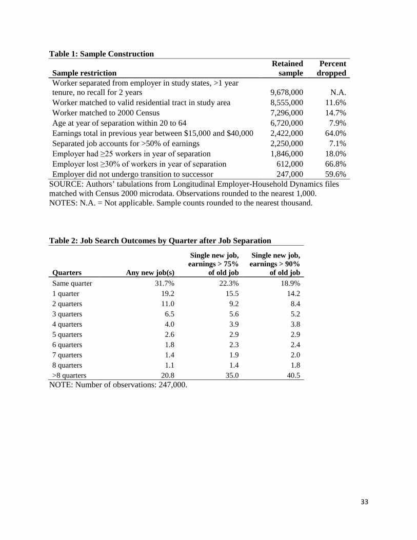
Table 1: Sample Construction

Sample restriction Retained

sample Percent

dropped Worker separated from employer in study states, >1 year tenure, no recall for 2 years 9,678,000 N.A. Worker matched to valid residential tract in study area 8,555,000 11.6% Worker matched to 2000 Census 7,296,000 14.7% Age at year of separation within 20 to 64 6,720,000 7.9% Earnings total in previous year between $15,000 and $40,000 2,422,000 64.0% Separated job accounts for >50% of earnings 2,250,000 7.1% Employer had ≥25 workers in year of separation 1,846,000 18.0% Employer lost ≥30% of workers in year of separation 612,000 66.8% Employer did not undergo transition to successor 247,000 59.6%

SOURCE: Authors’ tabulations from Longitudinal Employer-Household Dynamics files matched with Census 2000 microdata. Observations rounded to the nearest 1,000. NOTES: N.A. = Not applicable. Sample counts rounded to the nearest thousand. Table 2: Job Search Outcomes by Quarter after Job Separation

Quarters Any new job(s)

Single new job, earnings > 75%

of old job

Single new job, earnings > 90%

of old job

Same quarter 31.7% 22.3% 18.9% 1 quarter 19.2 15.5 14.2 2 quarters 11.0 9.2 8.4 3 quarters 6.5 5.6 5.2 4 quarters 4.0 3.9 3.8 5 quarters 2.6 2.9 2.9 6 quarters 1.8 2.3 2.4 7 quarters 1.4 1.9 2.0 8 quarters 1.1 1.4 1.8 >8 quarters 20.8 35.0 40.5

NOTE: Number of observations: 247,000.

33

Table 3: Summary Statistics for Sample of Displaced Workers Variable Mean Male 46.9% Female 53.1% White non-Hispanic 67.8% Black non-Hispanic 18.6% Hispanic 9.4% Other race non-Hispanic 4.3% Resides in central city (35.9% of full sample) White non-Hispanic 43.7% Black non-Hispanic 36.9% All others 19.4% Resides outside city, but in central county (28.0% of full sample) White non-Hispanic 76.7% Black non-Hispanic 11.6% All others 11.7% Resides outside central county (36.0% of full sample) White non-Hispanic 85.0% Black non-Hispanic 5.8% All others 9.2% Age 20 to 34 42.0% Age 35 to 44 46.2% Age 55 to 64 11.9% Married, Primary earner 13.0% Married, Secondary earner 11.8% Not-married 75.2% Industry: Goods-producing and distribution 39.5% Industry: Local services 28.3% Industry: Professional services 18.3% Industry: Education and public services 3.8% Industry: Health care services 10.1% Separated from job in 2000 16.0% Separated from job in 2001 27.6% Separated from job in 2002 20.7% Separated from job in 2003 14.4% Separated from job in 2004 12.4% Separated from job in 2005 9.0% Drive time to lost job <20 minutes 33.3% Drive time to lost job 20 to 40 minutes 37.3% Drive time to lost job >40 minutes 29.4% Household annual earnings $34,955 Annual earnings $27,282 Annual earnings at lost job $26,588 Earnings in displacement quarter $4,698 Lost job tenure (4 to 8+ quarters) 7.1 Job count 1.8 Census tract: Poverty rate in 2000 10.7% Census tract: Home ownership rate in 2000 66.7% Census tract: Public transit use rate in 2000 7.4% Census tract: Population per square mile in 2000 (1000s) 2.60 Census tract: Median housing unit age in 2000 39.7

NOTE: Number of observations: 247,000.

34

Table 4: Distribution of Job Accessibility

Sample Median Job Accessibility

All 0.036 White non-Hispanic -0.006 Black non-Hispanic 0.255 Hispanic -0.090 Other race non-Hispanic 0.273 Resides in central city 0.339 White non-Hispanic 0.439 Black non-Hispanic 0.333 Resides outside city, but in central county 0.098 White non-Hispanic 0.104 Black non-Hispanic -0.002 Resides outside central county -0.285 White non-Hispanic -0.333 Black non-Hispanic -0.045 Male 0.034 Female 0.037 Age 20 to 34 0.061 Age 35 to 54 0.021 Age 55 to 64 0.009 Previous earnings $15,000 to $29,999 0.035 Previous earnings $30,000 to $40,000 0.036 Industry: Goods-producing and distribution -0.020 Industry: Local services 0.076 Industry: Professional services 0.095 Industry: Education and public services 0.016 Industry: Health care services 0.075

NOTES: See equation (11) for the definition of the job accessibility. Number of observations: 247,000.

35

Table 5: Effect of Job Accessibility on Job Search Duration

Outcome: Any new job New job >75%

previous earnings New job >90%

previous earnings Variable 1 2 3

Job accessibility -0.050*** -0.066*** -0.083*** (0.009) (0.010) (0.010) Female 0.059*** 0.117*** 0.139*** (0.010) (0.011) (0.011) Black non-Hispanic 0.091*** 0.236*** 0.263*** (0.014) (0.016) (0.017) Hispanic 0.115*** 0.197*** 0.252*** (0.017) (0.020) (0.021) Other race non-Hispanic 0.233*** 0.238*** 0.259*** (0.023) (0.026) (0.027) Age 20 to 24 -0.216*** -0.134*** -0.115*** (0.016) (0.017) (0.018) Age 35 to 44 0.146*** 0.155*** 0.188*** (0.012) (0.014) (0.014) Age 45 to 54 0.377*** 0.423*** 0.469*** (0.013) (0.015) (0.015) Age 55 to 64 1.191*** 1.409*** 1.455*** (0.017) (0.020) (0.021) Log household annual earnings 0.123*** 0.077*** 0.065*** (0.013) (0.015) (0.015) Log annual earnings 1.469*** 0.947*** 0.649*** (0.063) (0.069) (0.070) Log annual earnings at lost job -2.042*** -1.323*** -0.797*** (0.060) (0.065) (0.066) Log earnings at lost job during 0.136*** 0.049*** 0.013*** separated quarter (0.005) (0.005) (0.005) Lost job tenure (4 to 8+ quarters) -0.020*** 0.010** 0.029*** (0.004) (0.005) (0.005) Job count -0.196*** -0.092*** -0.077*** (0.005) (0.005) (0.006) Auto travel time to lost job <20 min. 0.018* 0.054*** 0.078*** (0.011) (0.012) (0.013) Auto travel time to lost job >40 min. -0.022* -0.039*** -0.045*** (0.012) (0.014) (0.014) Tract: Poverty rate 0.145** 0.442*** 0.606*** (0.069) (0.080) (0.083) Tract: Homeownership rate -0.110*** -0.152*** -0.162*** (0.032) (0.036) (0.037) Tract: Population per square mile 8.658*** 5.103** 0.343 (2.179) (2.473) (2.567) Tract: Median home age (in 2000) 0.002*** 0.003*** 0.003*** (0.000) (0.000) (0.000) Industry: Local Services -0.492*** -0.551*** -0.540*** (0.012) (0.013) (0.014) Industry: Professional Services -0.239*** -0.401*** -0.454*** (0.013) (0.015) (0.016) Industry: Education and Public Services 0.478*** 0.361*** 0.237*** (0.027) (0.031) (0.032) Industry: Health Care Services -0.357*** -0.561*** -0.632*** (0.017) (0.020) (0.020) Pseudo R-squared 0.0266 0.0320 0.0260

NOTES: Tobit estimation with lower and upper censoring at zero and >8 quarters of job search; includes both metropolitan area by year controls and quarter of separation controls. Robust standard errors reported in parentheses. Number of observations: 247,000. R-squared for upper- and lower-censored Tobit models is the McFadden’s pseudo R-square measure. *** p<0.01, ** p<0.05, * p<0.1.

36

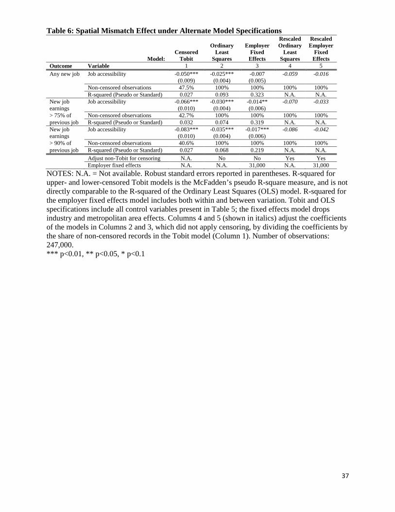
Table 6: Spatial Mismatch Effect under Alternate Model Specifications

Model: Censored

Tobit

Ordinary Least

Squares

Employer Fixed

Effects

Rescaled Ordinary

Least Squares

Rescaled Employer

Fixed Effects

Outcome Variable 1 2 3 4 5

Any new job Job accessibility -0.050*** -0.025*** -0.007 -0.059 -0.016 (0.009) (0.004) (0.005) Non-censored observations 47.5% 100% 100% 100% 100% R-squared (Pseudo or Standard) 0.027 0.093 0.323 N.A. N.A. New job Job accessibility -0.066*** -0.030*** -0.014** -0.070 -0.033 earnings (0.010) (0.004) (0.006) > 75% of Non-censored observations 42.7% 100% 100% 100% 100% previous job R-squared (Pseudo or Standard) 0.032 0.074 0.319 N.A. N.A. New job Job accessibility -0.083*** -0.035*** -0.017*** -0.086 -0.042 earnings (0.010) (0.004) (0.006) > 90% of Non-censored observations 40.6% 100% 100% 100% 100% previous job R-squared (Pseudo or Standard) 0.027 0.068 0.219 N.A. N.A.

Adjust non-Tobit for censoring N.A. No No Yes Yes Employer fixed effects N.A. N.A. 31,000 N.A. 31,000

NOTES: N.A. = Not available. Robust standard errors reported in parentheses. R-squared for upper- and lower-censored Tobit models is the McFadden’s pseudo R-square measure, and is not directly comparable to the R-squared of the Ordinary Least Squares (OLS) model. R-squared for the employer fixed effects model includes both within and between variation. Tobit and OLS specifications include all control variables present in Table 5; the fixed effects model drops industry and metropolitan area effects. Columns 4 and 5 (shown in italics) adjust the coefficients of the models in Columns 2 and 3, which did not apply censoring, by dividing the coefficients by the share of non-censored records in the Tobit model (Column 1). Number of observations: 247,000. *** p<0.01, ** p<0.05, * p<0.1

37

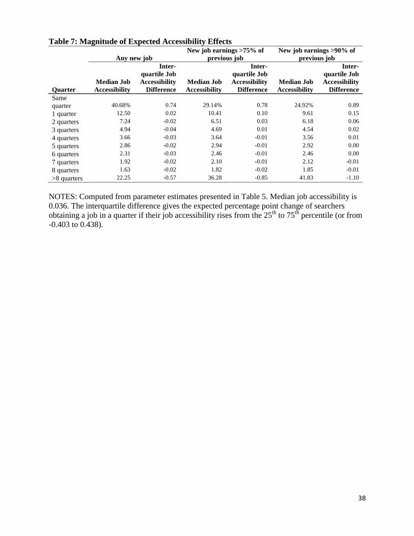
Table 7: Magnitude of Expected Accessibility Effects

Any new job New job earnings >75% of

previous job New job earnings >90% of

previous job

Quarter Median Job Accessibility

Inter-quartile Job Accessibility

Difference Median Job Accessibility

Inter-quartile Job Accessibility

Difference Median Job Accessibility

Inter-quartile Job Accessibility

Difference Same quarter 40.68% 0.74 29.14% 0.78 24.92% 0.89

1 quarter 12.50 0.02 10.41 0.10 9.61 0.15

2 quarters 7.24 -0.02 6.51 0.03 6.18 0.06

3 quarters 4.94 -0.04 4.69 0.01 4.54 0.02

4 quarters 3.66 -0.03 3.64 -0.01 3.56 0.01

5 quarters 2.86 -0.02 2.94 -0.01 2.92 0.00

6 quarters 2.31 -0.03 2.46 -0.01 2.46 0.00

7 quarters 1.92 -0.02 2.10 -0.01 2.12 -0.01

8 quarters 1.63 -0.02 1.82 -0.02 1.85 -0.01

>8 quarters 22.25 -0.57 36.28 -0.85 41.83 -1.10

NOTES: Computed from parameter estimates presented in Table 5. Median job accessibility is 0.036. The interquartile difference gives the expected percentage point change of searchers obtaining a job in a quarter if their job accessibility rises from the 25th to 75th percentile (or from -0.403 to 0.438).

38

Table 8: Effects of Job Accessibility, by Subsample Search outcome Job accessibility effect for subsample - Tobit estimation A: Race/Ethnicity White

non-Hispanic

Black non-Hispanic Hispanic

Other race non-

Hispanic Any new job -0.042*** -0.072*** -0.084*** 0.006 (0.011) (0.025) (0.025) (0.044) Earn > 75% previous

-0.072*** -0.083*** -0.069** 0.028

(0.013) (0.030) (0.029) (0.049) Earn > 90% previous

-0.086*** -0.116*** -0.066** -0.032

(0.013) (0.031) (0.030) (0.051) B: Sex and age Male Female Age 20-34 Age 35-54 Age 55-64 Any new job -0.049*** -0.051*** -0.031** -0.048*** -0.117*** (0.013) (0.012) (0.014) (0.012) (0.030) Earn > 75% previous

-0.048*** -0.082*** -0.043*** -0.062*** -0.180***

(0.014) (0.014) (0.015) (0.014) (0.040) Earn > 90% previous

-0.064*** -0.102*** -0.070*** -0.072*** -0.208***

(0.015) (0.015) (0.016) (0.014) (0.041) C: Household status and earnings

Married, Primary earner

Married, Secondary

earner Not-married

Previous earnings <

$30,000

Previous earnings ≥

$30,000 Any new job -0.039 -0.043 -0.054*** -0.035*** -0.067*** (0.026) (0.027) (0.010) (0.011) (0.015) Earn > 75% previous

-0.061** -0.076** -0.068*** -0.041*** -0.100***

(0.030) (0.032) (0.011) (0.013) (0.099) Earn > 90% previous

-0.070** -0.086*** -0.088*** -0.058*** -0.119***

(0.030) (0.032) (0.012) (0.013) (0.017) D: Industry Goods-

Producing Local

Services Professional

Services Education and Public Health Care

Any new job -0.080*** -0.009 -0.001 -0.113* -0.083** (0.012) (0.018) (0.023) (0.059) (0.033) Earn > 75% previous

-0.095*** -0.028 -0.046* -0.109 -0.080**

(0.014) (0.020) (0.026) (0.069) (0.035) Earn > 90% previous

-0.116*** -0.045** -0.061** -0.165** -0.076**

(0.015) (0.020) (0.027) (0.070) (0.035)

NOTES: Robust standard errors in parentheses. Each estimate is the variable of interest in an independent specification. Specifications include all control variables present in Table 5 except for indicators used in each panel to define industry, race/ethnicity, sex, or age. See Table 3 for sample share in each estimation model. *** p<0.01, ** p<0.05, * p<0.1.

39

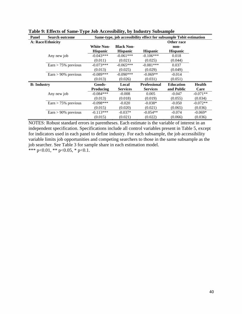
Table 9: Effects of Same-Type Job Accessibility, by Industry Subsample Panel Search outcome Same-type, job accessibility effect for subsample Tobit estimation A: Race/Ethnicity White Non-

Hispanic Black Non-

Hispanic Hispanic

Other race non-

Hispanic Any new job -0.043*** -0.061*** -0.106*** 0.018 (0.011) (0.021) (0.025) (0.044) Earn > 75% previous -0.073*** -0.065*** -0.081*** 0.037 (0.013) (0.025) (0.029) (0.049) Earn > 90% previous -0.089*** -0.090*** -0.069** -0.014 (0.013) (0.026) (0.031) (0.051)

B: Industry

Goods- Producing

Local Services

Professional Services

Education and Public

Health Care

Any new job -0.084*** -0.008 0.005 -0.047 -0.071** (0.013) (0.018) (0.019) (0.055) (0.034) Earn > 75% previous -0.098*** -0.020 -0.038* -0.050 -0.072** (0.015) (0.020) (0.021) (0.065) (0.036) Earn > 90% previous -0.113*** -0.037* -0.054** -0.074 -0.069* (0.015) (0.021) (0.022) (0.066) (0.036)

NOTES: Robust standard errors in parentheses. Each estimate is the variable of interest in an independent specification. Specifications include all control variables present in Table 5, except for indicators used in each panel to define industry. For each subsample, the job accessibility variable limits job opportunities and competing searchers to those in the same subsample as the job searcher. See Table 3 for sample share in each estimation model. *** p<0.01, ** p<0.05, * p<0.1.

40

Not Intended for Publication

APPENDIX A: Estimated Travel Time

This study makes use of point-to-point travel time estimates provided by Metropolitan

Planning Organizations (MPOs) in nine metropolitan areas. The MPOs use transportation

planning models to estimate driving and transit travel times between transportation analysis

zones at different times of day.34 We first translate the analysis zones into census tracts using

crosswalk files or proximity. For driving trips, we use only the travel times at the morning peak

period, when routes may be most congested. Reported public transit times may refer to trips by

bus, rail, tram, and other modes, depending on the metropolitan area.35

We impose several data edits to make the MPO data more representative of potential

travel times and more comparable across metropolitan areas. For both automobile and transit, we

assume zero travel time to jobs within a census tract. Because some MPOs effectively impose a

minimum transit time of approximately 10 minutes, we impose that minimum for all MPOs, but

also drop 5 minutes from all transit times to harmonize with auto travel, for which most MPOs

indicate zero vehicle access time.

We apply some deterministic imputations in the case of missing or invalid travel times.

For automobile travel, we impose a travel time one would infer from an assumed driving speed

of 20 miles per hour (great circle distance) - the average reported speed. Because of incomplete

transit networks, about two-thirds of tract pairs have no transit travel time. For both auto and

transit travel times that are slower than walking (assumed to be 3 miles per hour) we substitute

walking travel time for the reported or edited value. For potential “transit” commutes that are off

the network, we always impose the walking travel time, which makes travel time to all but the

nearest such tracts prohibitively long.

Table A1 presents summary statistics for travel times between directional, origin-

destination pairs. In addition to median travel times, the table reports median distances traveled

34 The MPO estimates of driving and transit travel times for large metropolitan areas are generally created by using a model that draws on the 2000 Census Transportation and Planning Package (CTPP) and local transit surveys. The models used by about 40 large US metropolitan areas are fairly similar, and are derived from one of two standard commercially-available sources. We thank the following MPO’s for providing us with commute times: Comprehensive Metropolitan Agency for Planning (Chicago), Greater Buffalo-Niagara Regional Transportation Council, Indianapolis Metropolitan Planning Organization, Mid-Ohio Regional Planning Commission (Columbus), Minneapolis Metropolitan Council, Northeast Ohio Areawide Coordinating Agency (Cleveland), Southeast Michigan Council of Governments (Detroit), Southwestern Pennsylvania Commission (Pittsburgh), Southeastern Wisconsin Regional Planning Commission (Milwaukee). 35 Although some MPOs provide information on “park-and-ride” commute times, where one drives to a transit stop, we only consider routes that are entirely transit-based.

41

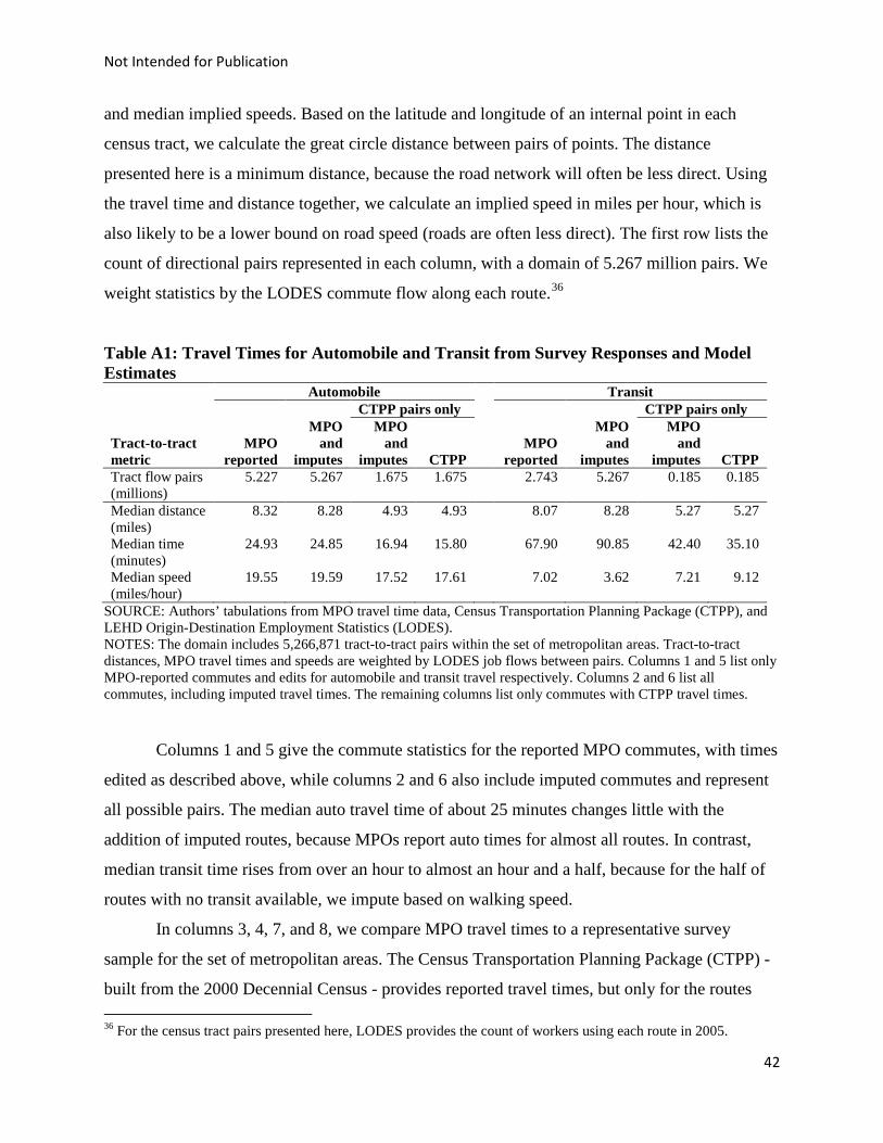
Not Intended for Publication

and median implied speeds. Based on the latitude and longitude of an internal point in each

census tract, we calculate the great circle distance between pairs of points. The distance

presented here is a minimum distance, because the road network will often be less direct. Using

the travel time and distance together, we calculate an implied speed in miles per hour, which is

also likely to be a lower bound on road speed (roads are often less direct). The first row lists the

count of directional pairs represented in each column, with a domain of 5.267 million pairs. We

weight statistics by the LODES commute flow along each route.36

Table A1: Travel Times for Automobile and Transit from Survey Responses and Model Estimates Automobile Transit CTPP pairs only CTPP pairs only

Tract-to-tract metric

MPO reported

MPO and

imputes

MPO and

imputes CTPP

MPO

reported

MPO and

imputes

MPO and

imputes CTPP Tract flow pairs (millions)

5.227 5.267 1.675 1.675 2.743 5.267 0.185 0.185

Median distance (miles)

8.32 8.28 4.93 4.93 8.07 8.28 5.27 5.27

Median time (minutes)

24.93 24.85 16.94 15.80 67.90 90.85 42.40 35.10

Median speed (miles/hour)

19.55 19.59 17.52 17.61 7.02 3.62 7.21 9.12

SOURCE: Authors’ tabulations from MPO travel time data, Census Transportation Planning Package (CTPP), and LEHD Origin-Destination Employment Statistics (LODES). NOTES: The domain includes 5,266,871 tract-to-tract pairs within the set of metropolitan areas. Tract-to-tract distances, MPO travel times and speeds are weighted by LODES job flows between pairs. Columns 1 and 5 list only MPO-reported commutes and edits for automobile and transit travel respectively. Columns 2 and 6 list all commutes, including imputed travel times. The remaining columns list only commutes with CTPP travel times.

Columns 1 and 5 give the commute statistics for the reported MPO commutes, with times

edited as described above, while columns 2 and 6 also include imputed commutes and represent

all possible pairs. The median auto travel time of about 25 minutes changes little with the

addition of imputed routes, because MPOs report auto times for almost all routes. In contrast,

median transit time rises from over an hour to almost an hour and a half, because for the half of

routes with no transit available, we impute based on walking speed.

In columns 3, 4, 7, and 8, we compare MPO travel times to a representative survey

sample for the set of metropolitan areas. The Census Transportation Planning Package (CTPP) -

built from the 2000 Decennial Census - provides reported travel times, but only for the routes

36 For the census tract pairs presented here, LODES provides the count of workers using each route in 2005.

42

Not Intended for Publication

actually traveled. Comparing CTPP travel times to MPO travel times provides an objective

evaluation of whether MPO travel times are a good representation of proximity. To minimize

measurement error from the survey travel times, we include only the census tract pairs with at

least 10 CTPP commutes by automobile or transit (also excluding within-tract commutes).37 For

the automobile pairs, we find an MPO median travel time of about 17 minutes, very close to the

CTPP median travel time of about 16 minutes. The transit travel times are more divergent, with

MPOs giving an average travel time of 42 minutes compared to only 35 minutes in CTPP. For

the same pairs of tracts, we find an MPO-CTPP correlation of 0.59 for automobile travel times

and 0.47 for transit travel times.

37 The CTPP automobile times are for commuters driving their own vehicle to work, leaving between 5:00 a.m. to 8:59 a.m. The CTPP transit times are for all other modes.

43

Not Intended for Publication

APPENDIX B: Individualized Travel Time Predictions

This section describes the development of the personalized prediction of transit use on

each potential commute route. The goal is to generate an expectation of whether a particular job

seeker would use automobile or transit to commute to a job in any tract. Because LEHD jobs

data and the MPO travel time data have no information on an individual’s commute choices, we

obtain commute choices from the 2000 Census long form responses – the Sample Edited Detail

File (SEDF). We estimate models of vehicle count and mode choice for respondents, and use the

parameter estimates to predict whether individuals in the job seeker dataset are likely to

commute by public transit. We use this predicted probability of auto or transit use to weight

accessibility to jobs in a tract, with accessibility of each mode depending on travel time for that

mode.

We combine the 2000 Census long form responses with the same datasets used to create

the sample of displaced workers. We first extract a sample of approximately 693,000 employed

respondents from the SEDF, who commute to a job in one of the nine metropolitan areas in our

sample.38 As with the displaced worker sample, we match these records to neighborhood,

commute time, and earnings data, with sample restrictions documented in Table B1.39 Because

we are focusing on mode choice, we limit the sample to residents of tracts with a feasible transit

option by requiring that at least 5 percent of residents report commuting by transit and that at

least 10 percent of routes to workplaces from that tract have an MPO transit travel time.40 These

restrictions reduce the sample by a cumulative 84.3 percent, resulting in a sample of

approximately 109,000 workers who might plausibly use either mode.

38 We are limited to records with a (de-duplicated) Personal Identification Key (PIK) and define employment based on an Employment Status Recode of ‘1’ and a Class of Worker of ‘1’ to ‘4’, including private sector and state and local government employees. We also limit to the age range in 2000 to 20-64, to those commuting (we exclude those working from home) to a job in an MPO county with LEHD data in 2000 (all but two study states), and to those with household information (a small share of records do not match to the household file). We exclude Michigan and Ohio cities from this estimation because they lack sufficient pre-2000 earnings histories. 39 We match by PIK to the Composite Person Record file of administrative residence data for the year 2000, and require residence in one of the MPO counties. We then match the respondent to MPO travel time data by place of work and place of residence census tract, and to the Summary File 1 neighborhood data by residence census tract. We limit to those having LEHD earnings in each quarter from 1999:2 to 2000:2, and require that earnings from 1999:2 to 2000:1 be between $15,000 and $40,000. 40 MPOs report estimated auto travel times between almost all tract pairs, but sometimes omit transit. Some MPOs have explained that they do not provide transit times when that mode is not available.

44

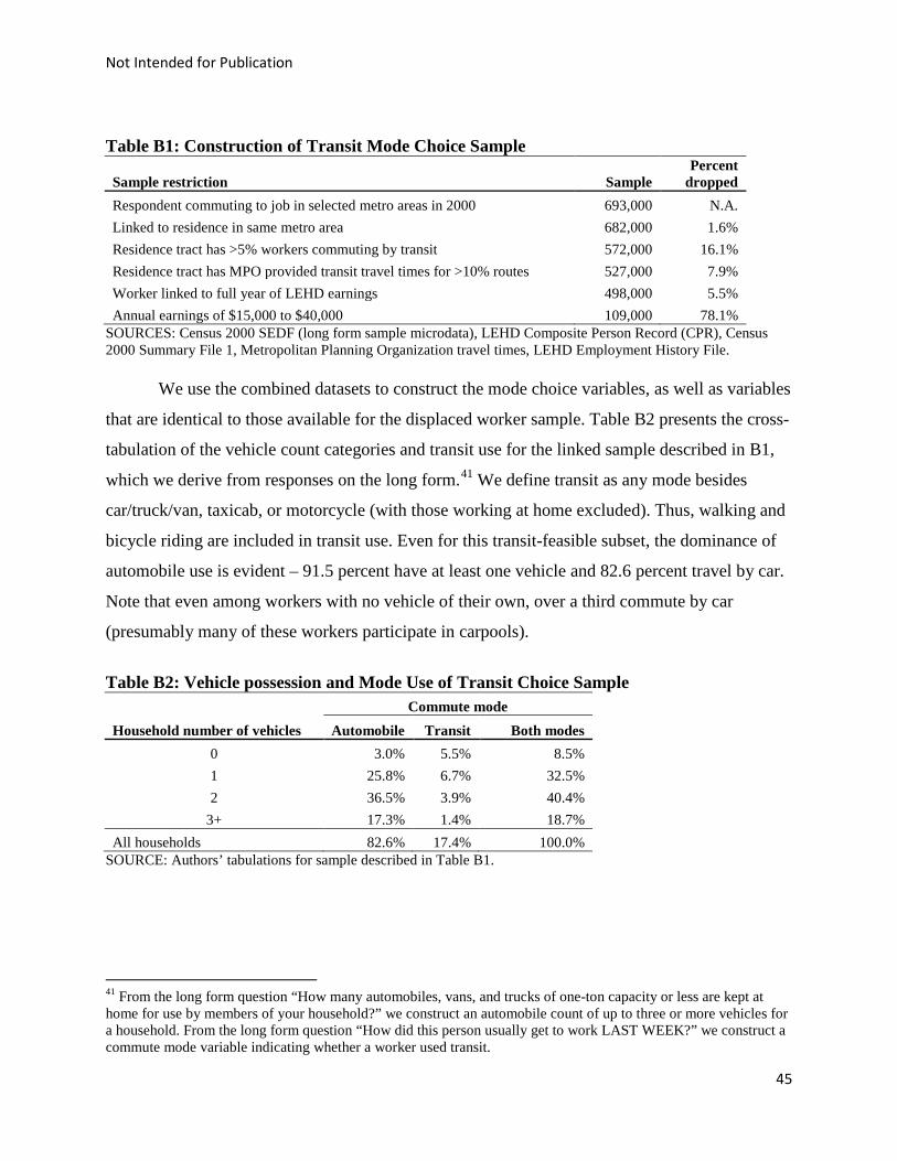
Not Intended for Publication

Table B1: Construction of Transit Mode Choice Sample

Sample restriction Sample Percent

dropped

Respondent commuting to job in selected metro areas in 2000 693,000 N.A.

Linked to residence in same metro area 682,000 1.6%

Residence tract has >5% workers commuting by transit 572,000 16.1%

Residence tract has MPO provided transit travel times for >10% routes 527,000 7.9%

Worker linked to full year of LEHD earnings 498,000 5.5%

Annual earnings of $15,000 to $40,000 109,000 78.1% SOURCES: Census 2000 SEDF (long form sample microdata), LEHD Composite Person Record (CPR), Census 2000 Summary File 1, Metropolitan Planning Organization travel times, LEHD Employment History File.

We use the combined datasets to construct the mode choice variables, as well as variables

that are identical to those available for the displaced worker sample. Table B2 presents the cross-

tabulation of the vehicle count categories and transit use for the linked sample described in B1,

which we derive from responses on the long form.41 We define transit as any mode besides

car/truck/van, taxicab, or motorcycle (with those working at home excluded). Thus, walking and

bicycle riding are included in transit use. Even for this transit-feasible subset, the dominance of

automobile use is evident – 91.5 percent have at least one vehicle and 82.6 percent travel by car.

Note that even among workers with no vehicle of their own, over a third commute by car

(presumably many of these workers participate in carpools).

Table B2: Vehicle possession and Mode Use of Transit Choice Sample Commute mode

Household number of vehicles Automobile Transit Both modes

0 3.0% 5.5% 8.5%

1 25.8% 6.7% 32.5%

2 36.5% 3.9% 40.4%

3+ 17.3% 1.4% 18.7%

All households 82.6% 17.4% 100.0% SOURCE: Authors’ tabulations for sample described in Table B1.

41 From the long form question “How many automobiles, vans, and trucks of one-ton capacity or less are kept at home for use by members of your household?” we construct an automobile count of up to three or more vehicles for a household. From the long form question “How did this person usually get to work LAST WEEK?” we construct a commute mode variable indicating whether a worker used transit.

45

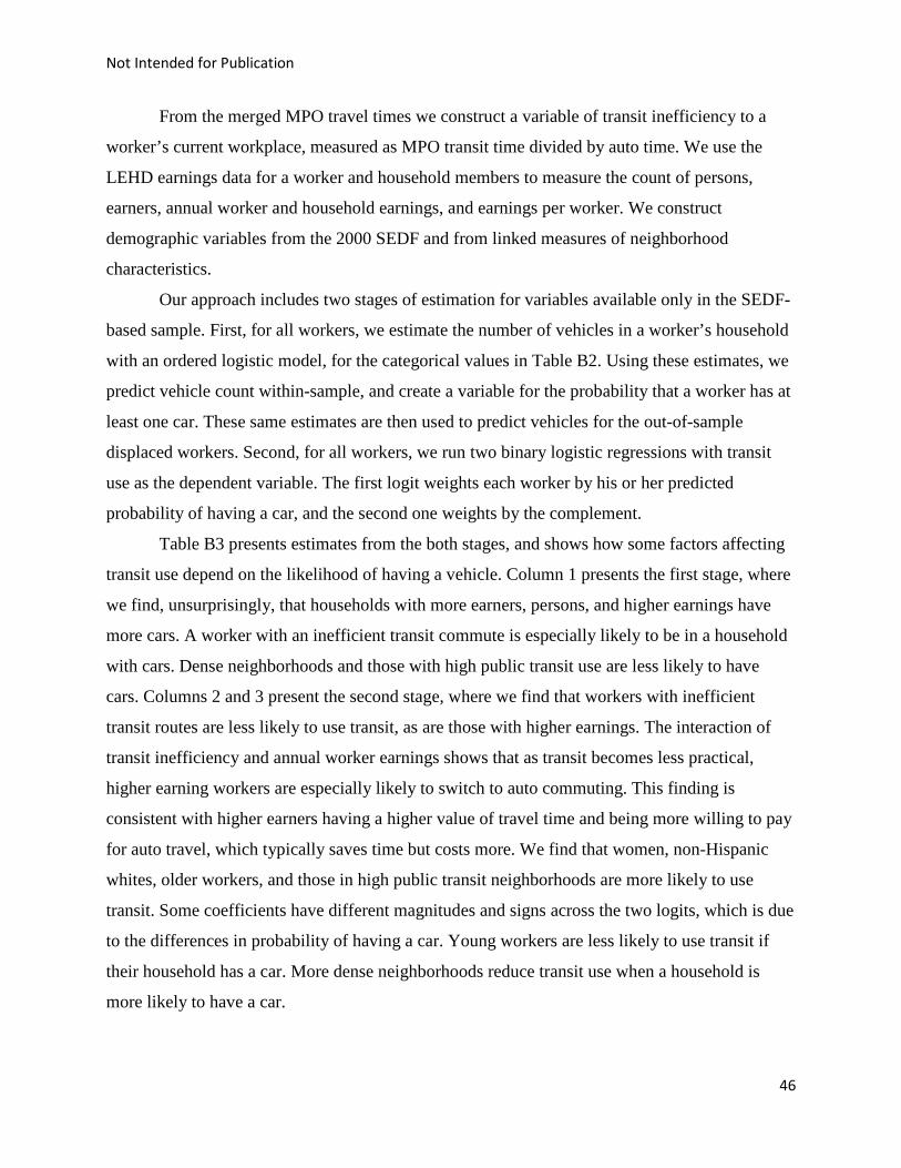
Not Intended for Publication

From the merged MPO travel times we construct a variable of transit inefficiency to a

worker’s current workplace, measured as MPO transit time divided by auto time. We use the

LEHD earnings data for a worker and household members to measure the count of persons,

earners, annual worker and household earnings, and earnings per worker. We construct

demographic variables from the 2000 SEDF and from linked measures of neighborhood

characteristics.

Our approach includes two stages of estimation for variables available only in the SEDF-

based sample. First, for all workers, we estimate the number of vehicles in a worker’s household

with an ordered logistic model, for the categorical values in Table B2. Using these estimates, we

predict vehicle count within-sample, and create a variable for the probability that a worker has at

least one car. These same estimates are then used to predict vehicles for the out-of-sample

displaced workers. Second, for all workers, we run two binary logistic regressions with transit

use as the dependent variable. The first logit weights each worker by his or her predicted

probability of having a car, and the second one weights by the complement.

Table B3 presents estimates from the both stages, and shows how some factors affecting

transit use depend on the likelihood of having a vehicle. Column 1 presents the first stage, where

we find, unsurprisingly, that households with more earners, persons, and higher earnings have

more cars. A worker with an inefficient transit commute is especially likely to be in a household

with cars. Dense neighborhoods and those with high public transit use are less likely to have

cars. Columns 2 and 3 present the second stage, where we find that workers with inefficient

transit routes are less likely to use transit, as are those with higher earnings. The interaction of

transit inefficiency and annual worker earnings shows that as transit becomes less practical,

higher earning workers are especially likely to switch to auto commuting. This finding is

consistent with higher earners having a higher value of travel time and being more willing to pay

for auto travel, which typically saves time but costs more. We find that women, non-Hispanic

whites, older workers, and those in high public transit neighborhoods are more likely to use

transit. Some coefficients have different magnitudes and signs across the two logits, which is due

to the differences in probability of having a car. Young workers are less likely to use transit if

their household has a car. More dense neighborhoods reduce transit use when a household is

more likely to have a car.

46

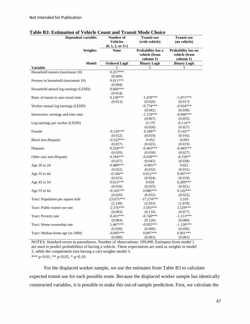
Not Intended for Publication

Table B3: Estimation of Vehicle Count and Transit Mode Choice Dependent variable: Number of

Vehicles (0, 1, 2, or 3+)

Transit use (with vehicle)

Transit use (no vehicle)

Weights: None Probability has a vehicle (from

column 1)

Probability has no vehicle (from

column 1) Model: Ordered Logit Binary Logit Binary Logit

Variable 1 2 3 Household earners (maximum 10) 0.237*** (0.009) Persons in household (maximum 10) 0.011*** (0.004) Household annual log earnings (LEHD) 0.666*** (0.014) Ratio of transit to auto travel time 0.130*** -1.478*** -1.071*** (0.013) (0.020) (0.017) Worker annual log earnings (LEHD) -0.774*** -0.934*** (0.042) (0.038) Interaction: earnings and time ratio -1.119*** -0.948*** (0.067) (0.055) Log earnings per worker (LEHD) -0.179 -0.114** (0.026) (0.027) Female -0.116*** 0.189** 0.142** (0.012) (0.019) (0.016) Black non-Hispanic -0.322*** -0.052 -0.093 (0.017) (0.025) (0.019) Hispanic 0.224*** -0.405*** -0.485*** (0.020) (0.030) (0.027) Other race non-Hispanic 0.184*** -0.038*** -0.150** (0.027) (0.041) (0.038) Age 20 to 24 0.489*** -0.005** 0.021 (0.022) (0.032) (0.031) Age 35 to 44 -0.106** 0.012*** 0.097*** (0.015) (0.024) (0.019) Age 45 to 54 0.015*** 0.059 0.209*** (0.016) (0.025) (0.021) Age 55 to 64 -0.165*** 0.080*** 0.142*** (0.020) (0.032) (0.025) Tract: Population per square mile -23.675*** -17.274*** 3.319 (2.149) (2.933) (1.678) Tract: Public transit use rate -2.576*** 3.593*** 3.129*** (0.083) (0.116) (0.077) Tract: Poverty rate 0.431*** -0.740*** -1.113*** (0.083) (0.120) (0.080) Tract: Home ownership rate 1.467*** -0.955*** -1.128*** (0.039) (0.060) (0.050) Tract: Median home age (in 2000) -0.005*** 0.007*** 0.001*** (0.000) (0.001) (0.001) NOTES: Standard errors in parentheses. Number of observations: 109,000. Estimates from model 1 are used to predict probabilities of having a vehicle. These expectations are used as weights in model 2, while the complement (not having a car) weights model 3. *** p<0.01, ** p<0.05, * p<0.10.

For the displaced worker sample, we use the estimates from Table B3 to calculate

expected transit use for each possible route. Because the displaced worker sample has identically

constructed variables, it is possible to make this out-of-sample prediction. First, we calculate the

47

Not Intended for Publication

expected probability of the job seeker’s household having a vehicle, using the estimates from

Column 1. Then, for the same worker, we calculate probability of transit use with the estimates

in Column 2 and 3. Lastly, we use the expected probability of having a car to create a weighted

average of the probability of using public transit on each route. This probability of transit use

feeds into the predicted job accessibility ratio calculation in equation (11). Using the same rules

as described above for transit feasibility, we only apply these probabilities to workers residing in

the 41 percent of Census tracts with feasible transit options. We assume all other workers posses

a car and drive to potential job opportunities.

The results presented here are informative about the factors affecting transit use.

However, as is explained before, auto availability and usage is widespread. Ultimately, the

minimal use of transit limits the efficacy of this approach in adding personalized variation to

travel time measures.

48

Not Intended for Publication

APPENDIX C: Robustness Tests

Table C1 presents the variance/covariance and correlations for various job accessibility

ratios with varied assumptions on the use of automobile and transit, providing some intuition on

the importance of equation (11) employing predicted mode use. The first two measures,

calculated assuming either �̂�𝑖𝑗𝑘(auto) = 1 or �̂�𝑖𝑗𝑘(transit) = 1 are only weakly correlated (0.25),

suggesting that in theory, incorporating transit usage could add information to the job

accessibility measure. However, the predicted job access ratio, which incorporates the weighted

likelihood of using each mode, turns out to mostly composed of variation from automobile

commutes. This should not be very surprising, given that only 7 percent of workers use transit in

the relevant residential census tracts. In Column 3 of each panel, note that the contribution of

auto access to the combined measure accounts for most of the variation and has a correlation of

0.96, while the transit contribution has a correlation of only 0.21. Column 4 shows that these

auto and transit contributions are actually slightly negatively related to one another. The last

element of each panel, which is used for all the main results in this paper, gives a predicted

access ratio where only workers in tracts with a feasible transit option are given any possibility

of using transit.

Table C1: Relationship of Access Ratio Measures, by Travel Time

Auto Transit Predicted Predicted

Auto Predicted

Transit

Predicted, Feasible Transit

Panel A: Covariance

Automobile 0.36

Transit 0.09 0.37

Predicted 0.35 0.12 0.35

Predicted auto contribution 0.36 0.04 0.35 0.37

Predicted transit contribution 0.03 0.22 0.05 -0.01 0.15

Predicted (only feasible transit) 0.35 0.11 0.35 0.35 0.04 0.35

Panel B: Correlation

Automobile 1.00

Transit 0.25 1.00

Predicted 0.99 0.32 1.00

Predicted auto contribution 0.98 0.12 0.96 1.00

Predicted transit contribution 0.12 0.91 0.22 -0.03 1.00

Predicted (only feasible transit) 0.99 0.29 1.00 0.97 0.18 1.00 SOURCE: Authors’ tabulations from Longitudinal Employer-Household Dynamics files matched with Census 2000 microdata. NOTE: Number of observations: 247,000.

49

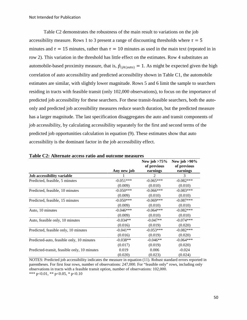
Not Intended for Publication

Table C2 demonstrates the robustness of the main result to variations on the job

accessibility measure. Rows 1 to 3 present a range of discounting thresholds where 𝜏 = 5

minutes and 𝜏 = 15 minutes, rather than 𝜏 = 10 minutes as used in the main text (repeated in in

row 2). This variation in the threshold has little effect on the estimates. Row 4 substitutes an

automobile-based proximity measure, that is, �̂�𝑖𝑗𝑘(auto) = 1. As might be expected given the high

correlation of auto accessibility and predicted accessibility shown in Table C1, the automobile

estimates are similar, with slightly lower magnitude. Rows 5 and 6 limit the sample to searchers

residing in tracts with feasible transit (only 102,000 observations), to focus on the importance of

predicted job accessibility for these searchers. For these transit-feasible searchers, both the auto-

only and predicted job accessibility measures reduce search duration, but the predicted measure

has a larger magnitude. The last specification disaggregates the auto and transit components of

job accessibility, by calculating accessibility separately for the first and second terms of the

predicted job opportunities calculation in equation (9). These estimates show that auto

accessibility is the dominant factor in the job accessibility effect.

Table C2: Alternate access ratio and outcome measures

Any new job

New job >75% of previous

earnings

New job >90% of previous

earnings Job accessibility variable 1 2 3 Predicted, feasible, 5 minutes -0.051*** -0.065*** -0.082*** (0.009) (0.010) (0.010) Predicted, feasible, 10 minutes -0.050*** -0.066*** -0.083*** (0.009) (0.010) (0.010) Predicted, feasible, 15 minutes -0.050*** -0.069*** -0.087*** (0.009) (0.010) (0.010) Auto, 10 minutes -0.046*** -0.064*** -0.082*** (0.009) (0.010) (0.010) Auto, feasible only, 10 minutes -0.034** -0.047** -0.074*** (0.016) (0.019) (0.020) Predicted, feasible only, 10 minutes -0.041** -0.053*** -0.082*** (0.016) (0.019) (0.020) Predicted-auto, feasible only, 10 minutes -0.038** -0.046** -0.064*** (0.017) (0.019) (0.020) Predicted-transit, feasible only, 10 minutes 0.019 0.006 -0.024 (0.020) (0.023) (0.024) NOTES: Predicted job accessibility indicates the measure in equation (11). Robust standard errors reported in parentheses. For first four rows, number of observations: 247,000. For “feasible only” rows, including only observations in tracts with a feasible transit option, number of observations: 102,000. *** p<0.01, ** p<0.05, * p<0.10

50