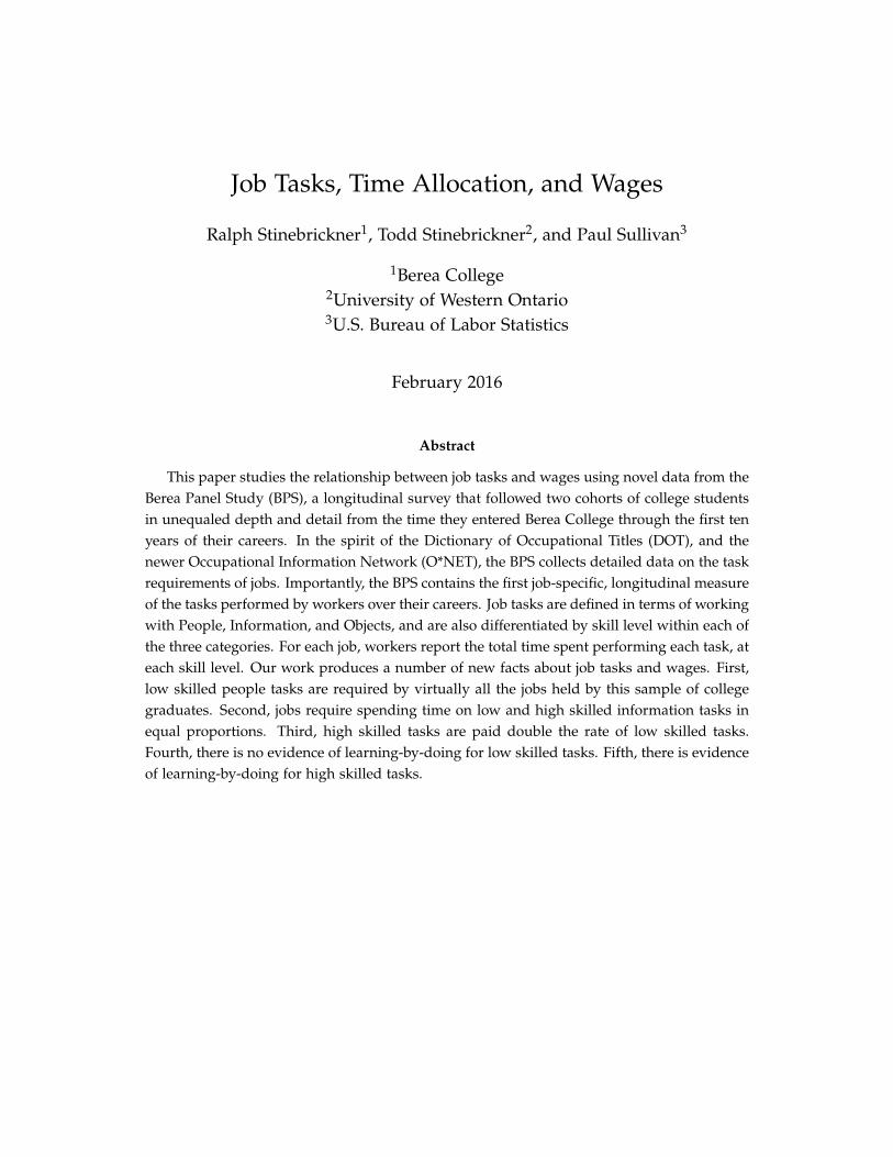
Job Tasks, Time Allocation, and Wages

Ralph Stinebrickner1, Todd Stinebrickner2, and Paul Sullivan3

1Berea College2University of Western Ontario3U.S. Bureau of Labor Statistics

February 2016

Abstract

This paper studies the relationship between job tasks and wages using novel data from theBerea Panel Study (BPS), a longitudinal survey that followed two cohorts of college studentsin unequaled depth and detail from the time they entered Berea College through the first tenyears of their careers. In the spirit of the Dictionary of Occupational Titles (DOT), and thenewer Occupational Information Network (O*NET), the BPS collects detailed data on the taskrequirements of jobs. Importantly, the BPS contains the first job-specific, longitudinal measureof the tasks performed by workers over their careers. Job tasks are defined in terms of workingwith People, Information, and Objects, and are also differentiated by skill level within each ofthe three categories. For each job, workers report the total time spent performing each task, ateach skill level. Our work produces a number of new facts about job tasks and wages. First,low skilled people tasks are required by virtually all the jobs held by this sample of collegegraduates. Second, jobs require spending time on low and high skilled information tasks inequal proportions. Third, high skilled tasks are paid double the rate of low skilled tasks.Fourth, there is no evidence of learning-by-doing for low skilled tasks. Fifth, there is evidenceof learning-by-doing for high skilled tasks.

1 Introduction

Characterizing the tasks that a worker performs on-the-job is critical for understanding the de-

termination of wages both over the lifecycle and in the cross section. The notion that worker

productivity, and therefore wages, will depend directly on current job tasks is supported empiri-

cally by a large literature that explores the existence of wage differentials across employers (Man-

ning, 2003), industries (Gibbons and Katz, 1992), occupations (Heckman and Sedlacek, 1985), and

worker skill levels (Acemoglu and Autor, 2011; Autor and Dorn, 2013). However, as emphasized

by the learning-by-doing model of human capital formation (Becker, 1964), one’s productivity

today will also depend on past tasks.1

In this paper, we provide new information about wage determination over the early part of the

lifecycle by taking advantage of unique new data from the Berea Panel Study that was collected

specifically to address well-known current limitations associated with the measurement of job

tasks. The data provide direct measures of the time spent on different job tasks over the ten

year period immediately after students graduate from college. Using these data, we estimate the

impact of current job tasks on wages. In addition, we construct new proxies for human capital

- the cumulative amount of time over the career spent performing each task - and use these

variables to examine the importance of learning-by-doing by workers.2

One commonly employed approach for providing evidence about the relationship between

tasks and wages involves examining wage differences across groups of jobs that, from an intuitive

standpoint, might be expected to involve similar types of activities. This approach has the virtue

of being feasible as long as a researcher has access to occupational codes or other information

that can reasonably be used to form job groupings. However, when the number of chosen job

groupings is small (e.g., in the extreme when one divides jobs into blue-collar/white collar),

workers may be performing quite different tasks within the specified job groups. In this case,

the job groupings may explain relatively little variation in observed wages, and, therefore, the

approach may not reveal the full importance of tasks. While increasing the number of groups

1Motivated by this theory, a vast empirical literature examines questions such as whether human capital tends tobe general and transferable across all jobs (Mincer, 1974), or specific to occupations or industries. See Neal (1995)and Parent (2000) for studies of industry specific human capital, and Kambourov and Manovskii (2009) and Sullivan(2010) for evidence of occupation specificity.

2We use the term learning-by-doing loosely. A situation where past tasks are related to current work performancecould also arise because of formal on-the-job-training.

1

may allow the specified job groupings to explain more of the variation in wages, this increase may

lead to a situation where it is not possible to describe, or even understand, why wages vary across

groups because differences in jobs tasks across groups are not being explicitly characterized.

These types of difficulties have motivated a burgeoning, recent literature interested in charac-

terizing the tasks performed on jobs directly using measures of the type found in the Dictionary

of Occupational Titles (DOT) or the newer Occupational Information Network (O*NET).3 Un-

fortunately, while recent work has established the appeal of this approach, well-known data

limitations exist in practice and these limitations are particularly salient in our context.

The most fundamental data limitation is that no longitudinal surveys have collected DOT or

O*NET type information directly for individual workers. As a result, it is necessary to use the

DOT or O*NET databases to assign job tasks to workers in each year. The potential problems

with this matching approach have been well-recognized. Because a worker’s exact job description

is not typically observed, matching must take place on the basis of a worker’s occupation (which

is observed). As a result, in practice all workers in the same (typically three digit) occupation

are assigned the same tasks. Taking advantage of rare cross-sectional data that allows job tasks

to be observed at the individual job-level, Robinson (2011) and Autor and Handel (2013) show

that it is problematic to characterize tasks using this matching approach because tasks vary

significantly within three-digit occupations.4 It is immediately evident that, without access to

longitudinal data that accurately characterizes job tasks over multiple years, it will not be possible

to understand the role that past work activities play in determining current wages. However, the

absence of such longitudinal data may make it difficult to even understand the effect of current

tasks on wages (even in the rare case where one has accurate cross-sectional measures of tasks),

because what a person does on-the-job today tends to be strongly related to what he did in the

past. In addition, without longitudinal data, it is also not possible to take advantage of estimators

(e.g., fixed effects) that utilize within-person variation across years to remove the influence of

3See, for example Poletaev and Robinson (2008), Gathmann and Schönberg (2010), Yamaguchi (2010), and Sanders(2014).

4Robinson (2011) uses the one year (1971) of CPS data in which an analyst assigned DOT tasks to jobs at theindividual level to show that there is a large amount of variation within three digit occupations in the tasks thatare performed on jobs. Autor and Handel (2013) also find substantial variation in tasks within an occupation whenthey collect individual level information about tasks as part of the Princeton Data Improvement Initiative survey andshow that this information is an important predictor of earnings even after conditioning on occupation. The UK Skillssurvey and new LISA survey (Canada) are the only other two datasets that provide cross-sectional information aboutjob tasks at the level of an individual worker-job.

2

unobserved ability or other unobserved, permanent factors.5

A second fundamental limitation arises because the questions used to describe tasks in the

DOT or O*NET are typically of a qualitative nature (important, very important, etc.), and, in

addition, may not always distinguish between the skill level at which a task is performed and the

amount of time that is spent on the task. This limitation often causes difficulty in interpreting

parameter estimates. In the longitudinal setting of interest here, it also makes it conceptually

difficult to know how to aggregate a person’s task usage over multiple years.6

In this paper we provide new evidence about how earnings are affected by current and past

job tasks by taking advantage of unique longitudinal data that was collected specifically to ad-

dress the two major task-measurement limitations described in the previous two paragraphs.

The data come from the Berea Panel Study (BPS), which followed two cohorts of students very

closely from the time of college entrance past the age of thirty.

The BPS task measures are in the spirit of some of the task information available in the DOT,

describing the manner in which tasks relate to People, Information, and Objects.7 Related to

the discussion above, the crucial feature of the data collection is that the task information comes

directly from the worker, providing a rare measure of what the worker is actually doing on his

job. The fact that this information was collected yearly starting at the time of graduation allows

us to construct the first longitudinal dataset containing job-level task information for individual

workers. Another unique feature of our task measures comes from collecting time allocation

5From a substantive standpoint, the implications of this measurement problem can also be seen immediately bynoting that task measures are not able to provide any insight into the substantial variation in earnings that is presentacross workers in the same occupation or across time for a worker who stays in the same occupation. Researchershave noted that the importance of having direct individual-level task information is likely to be strongest when oneis investigating issues that require longitudinal data. When describing the (not realized) possibility of collecting thistype of longitudinal information as part of the British Skill survey, Green et al. (2006) write: “such a longitudinalstudy...would enable a huge leap in our understanding of the processes of skills development...”

6For example, an estimate may show that moving from a particular task being “not important” to the task being“important” has a sizable affect on earnings, but it may be hard to understand what type of change in job activitieswould lead a person to report important rather than not important. Similarly, if a task is important in one year andnot important in the next year, it is hard to know how to characterize the cumulative importance of the task overthe two years. In practice, factor analysis is often used to summarize a large number of DOT or O*NET questions interms of a smaller number of factors (e.g., cognitive or manual). The same issues remain in this case. The weightscharacterizing the importance of cognitive and manual tasks for a particular occupation are informative about thetasks in that occupation relative to other jobs, but do not have a clear interpretation in terms of the level of tasks beingperformed. Further complicating interpretation, it is typically the case that some DOT and O*NET questions used toidentify the factor are more related to task level and others are more related to how frequently a task is performed.These issues also imply that it is difficult to know how to aggregate the weights that come out of factor models overmultiple years.

7We have condensed the number of categories within People, Information, and Objects relative to the DOT, andhave also written the categories so that they are ordered in terms of the level of the tasks being performed.

3

information related to the task measures. The BPS collected data detailing the percentage of

work time in a year that is spent in the People, Information, and Objects task categories. Within

each general task category, respondents report the percentage of time that is spent performing

different sub-tasks, which are ordered by skill level. Using these data, we are able to determine

the amount of time that each worker spends on both high and low skilled tasks, for each of

the three task categories (People, Information, and Objects). For each worker, summing each of

the six task variables over time, after weighting by hours worked, provides a direct measure of

task-specific work experience at each point of the career.

Our results examine up to ten years of labor market data. The descriptive results in Section 3

represent the first time it is has been possible to quantify, using explicit time measures, how

workers are spending time on their particular jobs. As examples of our findings: 1) within each

task, while in aggregate people spend equal amounts of time on high and low skilled work,

there is substantial heterogeneity, 2) even for this sample of college graduates, very few people

are able to avoid low skilled people tasks, 3) relative to people and object tasks, high and low

skilled information tasks are more likely to be performed in approximately equal proportions.

Our primary results appear in Section 4 where our models of wage determination take into

account both current and past tasks. The primary challenge to viewing the relationships between

(current and past) tasks and wages as causal comes from the possibility that students with more

human capital (or unobserved ability) at the time of college graduation are more likely to work in

in different types of jobs (e.g., jobs that require high-skilled tasks) than students with less human

capital at the time of college graduation. We first present results which attempt to address this

concern by conditioning on observable characteristics. We note that our study of one school

may help contribute to the appeal of the conditioning approach because it allows us to condition

on a measure of initial human capital, college GPA, that is directly comparable across students

in our sample. However, we also estimate a fixed effect model which controls for permanent,

unobserved differences across people. The big picture takeaways from the estimation of the two

models, which rely on very different identification strategies, are remarkably similar. Our first

main finding is that current job tasks play a large role in determining wages. In particular, there

is a large wage premium for performing high skilled work: high skilled tasks are paid roughly

double the rate of low skilled tasks. Our second main finding is that there is no evidence of

4

learning-by-doing for low skilled tasks, but there is strong evidence of learning-by-doing for

high skilled tasks. Our third main finding is that not all types of high skilled tasks (i.e., People,

Information, and Objects) play the same role in the determination of wages. We find that working

in high skilled people tasks in the present and/or in the past plays an important role, but that

that the influence of working in high skilled information tasks in the present and/or in the past

is especially large.

From a methodological standpoint, our results indicate that longitudinal data on tasks is

crucial for understanding a variety of important issues, including those related to wage growth.

In terms of direct guidance about survey questions, our time allocation measures represent a

promising way to characterize the type of work required by jobs and lead to natural proxies

for on-the-job human capital accumulation, which appear to be an improvement over existing

proxies (such as years of work experience). In addition, differentiating tasks by skill level is

crucial in order to understand wage differences across workers.

2 Data

This section provides general information about the Berea Panel Study (2.1) and explains how

job tasks are measured in this dataset (2.2).

2.1 The Berea Panel Study

Designed and administered by Todd Stinebrickner and Ralph Stinebrickner, the Berea Panel

Study (BPS) is a longitudinal survey that was initiated to provide more detailed information

about the college and early post-college periods than had previously been available. The project

involves surveying students who entered Berea College in the fall of 2000 and the fall of 2001

approximately sixty times from the time they entered college through 2014. In this paper, we

focus on understanding the evolution of earnings for individuals who graduated, by taking

advantage of post-college surveys that were collected annually after students left school. More

than ninety percent of all graduates in the two BPS cohort years completed one or more of these

annual surveys, and the response rate on the these surveys leveled off at approximately eighty-

two percent until 2011 before declining slightly. To avoid the need to impute crucial information,

our analysis uses all yearly observations from the time of graduation until either the end of the

5

sample period (2014) or the year that the person fails to complete a survey, whichever comes first.

For the 546 individuals in our sample, the maximum number of yearly observations is 10 and

the average number of yearly observations is 7.1.

Berea College is unique in certain respects that have been discussed in previous work. For

example, the school has a focus on providing educational opportunities to students from rela-

tively low income backgrounds. As such, as has been noted in our previous work that has used

the BPS to study other issues (see e.g., Stinebrickner and Stinebrickner 2003; 2006; 2012; 2013),

it is necessary to be appropriately cautious about the exact extent to which the results from our

case study would generalize to other demographic groups or to other specific institutions. How-

ever, important for the notion that the basic lessons from our work are pertinent for thinking

about what takes place elsewhere, Berea operates under a standard liberal arts curriculum, and

the students at Berea are similar in academic quality to, for example, students at the University

of Kentucky (S&S, 2008). In addition, earlier work found that academic decisions at Berea look

very similar to decisions made elsewhere. For example, dropout rates are similar to those found

elsewhere (for students from similar income backgrounds) and patterns of major choice and

major-switching at Berea are similar in spirit to those found in the NLSY by Arcidiacono (2004).

Further, even putting aside the obvious issue of data collection feasibility, there are benefits of

studying one school. In particular, the ability to hold school quality constant is beneficial for

a variety of reasons, including that it makes academic measures such as college GPA directly

comparable across individuals. An additional virtue of our data collection is that it allows us to

examine individuals starting at the very beginning of their careers.

This paper is made possible by merging the unique survey data from the early portion of

an individual’s working life with detailed administrative data. The administrative data provides

basic demographic information as well as academic information that is necessary to characterize

one’s human capital at the time the worker enters the workforce. Panel A in Table 1 shows that

64 percent of the sample is female, 15 percent of the sample is black, and the average college

grade point average (GPA) is 3.17. Pooling all observations across the full sample period, the

average hourly wage, in 2005 dollars, is $15.42, the average work week is 39.58 hours with 43

percent of jobs reporting exactly a 40 hour week.

6

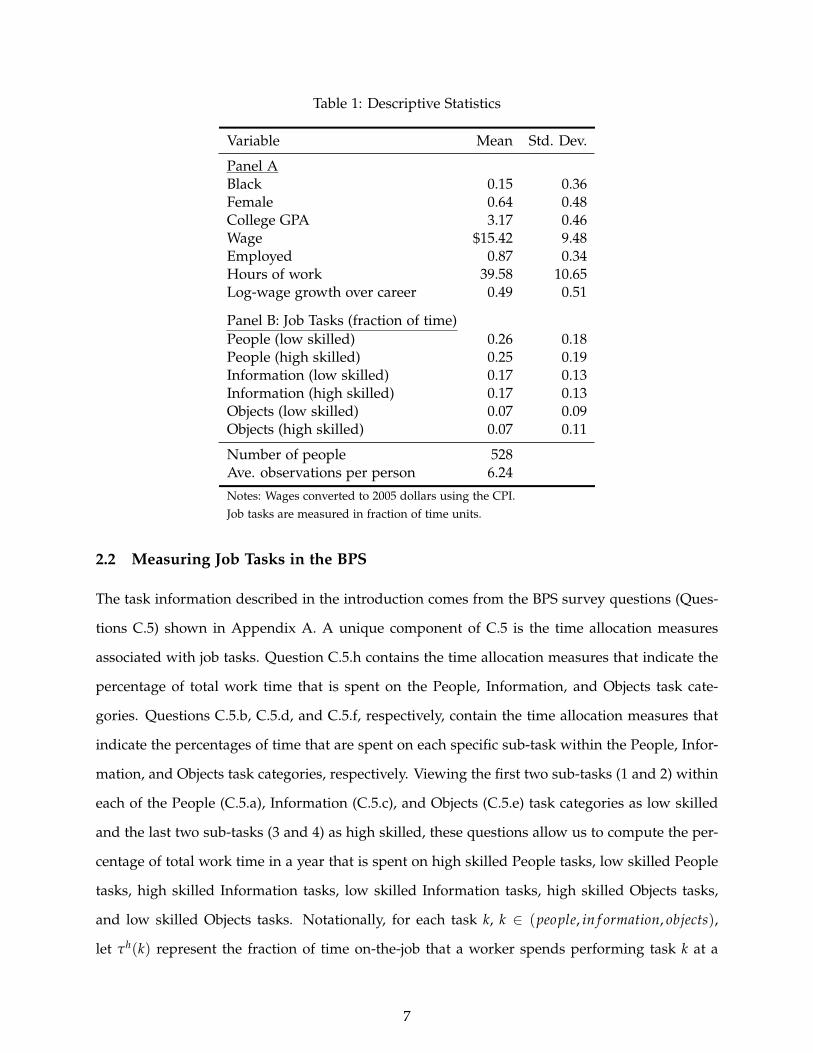
Table 1: Descriptive Statistics

Variable Mean Std. Dev.

Panel ABlack 0.15 0.36Female 0.64 0.48College GPA 3.17 0.46Wage $15.42 9.48Employed 0.87 0.34Hours of work 39.58 10.65Log-wage growth over career 0.49 0.51

Panel B: Job Tasks (fraction of time)People (low skilled) 0.26 0.18People (high skilled) 0.25 0.19Information (low skilled) 0.17 0.13Information (high skilled) 0.17 0.13Objects (low skilled) 0.07 0.09Objects (high skilled) 0.07 0.11

Number of people 528Ave. observations per person 6.24

Notes: Wages converted to 2005 dollars using the CPI.Job tasks are measured in fraction of time units.

2.2 Measuring Job Tasks in the BPS

The task information described in the introduction comes from the BPS survey questions (Ques-

tions C.5) shown in Appendix A. A unique component of C.5 is the time allocation measures

associated with job tasks. Question C.5.h contains the time allocation measures that indicate the

percentage of total work time that is spent on the People, Information, and Objects task cate-

gories. Questions C.5.b, C.5.d, and C.5.f, respectively, contain the time allocation measures that

indicate the percentages of time that are spent on each specific sub-task within the People, Infor-

mation, and Objects task categories, respectively. Viewing the first two sub-tasks (1 and 2) within

each of the People (C.5.a), Information (C.5.c), and Objects (C.5.e) task categories as low skilled

and the last two sub-tasks (3 and 4) as high skilled, these questions allow us to compute the per-

centage of total work time in a year that is spent on high skilled People tasks, low skilled People

tasks, high skilled Information tasks, low skilled Information tasks, high skilled Objects tasks,

and low skilled Objects tasks. Notationally, for each task k, k ∈ (people, in f ormation, objects),

let τh(k) represent the fraction of time on-the-job that a worker spends performing task k at a

7

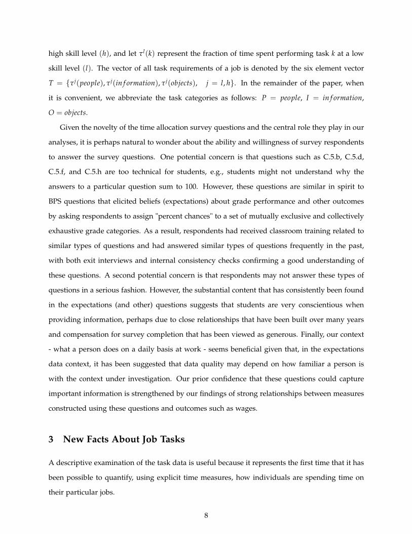
high skill level (h), and let τl(k) represent the fraction of time spent performing task k at a low

skill level (l). The vector of all task requirements of a job is denoted by the six element vector

T = {τ j(people), τ j(in f ormation), τ j(objects), j = l, h}. In the remainder of the paper, when

it is convenient, we abbreviate the task categories as follows: P = people, I = in f ormation,

O = objects.

Given the novelty of the time allocation survey questions and the central role they play in our

analyses, it is perhaps natural to wonder about the ability and willingness of survey respondents

to answer the survey questions. One potential concern is that questions such as C.5.b, C.5.d,

C.5.f, and C.5.h are too technical for students, e.g., students might not understand why the

answers to a particular question sum to 100. However, these questions are similar in spirit to

BPS questions that elicited beliefs (expectations) about grade performance and other outcomes

by asking respondents to assign "percent chances" to a set of mutually exclusive and collectively

exhaustive grade categories. As a result, respondents had received classroom training related to

similar types of questions and had answered similar types of questions frequently in the past,

with both exit interviews and internal consistency checks confirming a good understanding of

these questions. A second potential concern is that respondents may not answer these types of

questions in a serious fashion. However, the substantial content that has consistently been found

in the expectations (and other) questions suggests that students are very conscientious when

providing information, perhaps due to close relationships that have been built over many years

and compensation for survey completion that has been viewed as generous. Finally, our context

- what a person does on a daily basis at work - seems beneficial given that, in the expectations

data context, it has been suggested that data quality may depend on how familiar a person is

with the context under investigation. Our prior confidence that these questions could capture

important information is strengthened by our findings of strong relationships between measures

constructed using these questions and outcomes such as wages.

3 New Facts About Job Tasks

A descriptive examination of the task data is useful because it represents the first time that it has

been possible to quantify, using explicit time measures, how individuals are spending time on

their particular jobs.

8

9

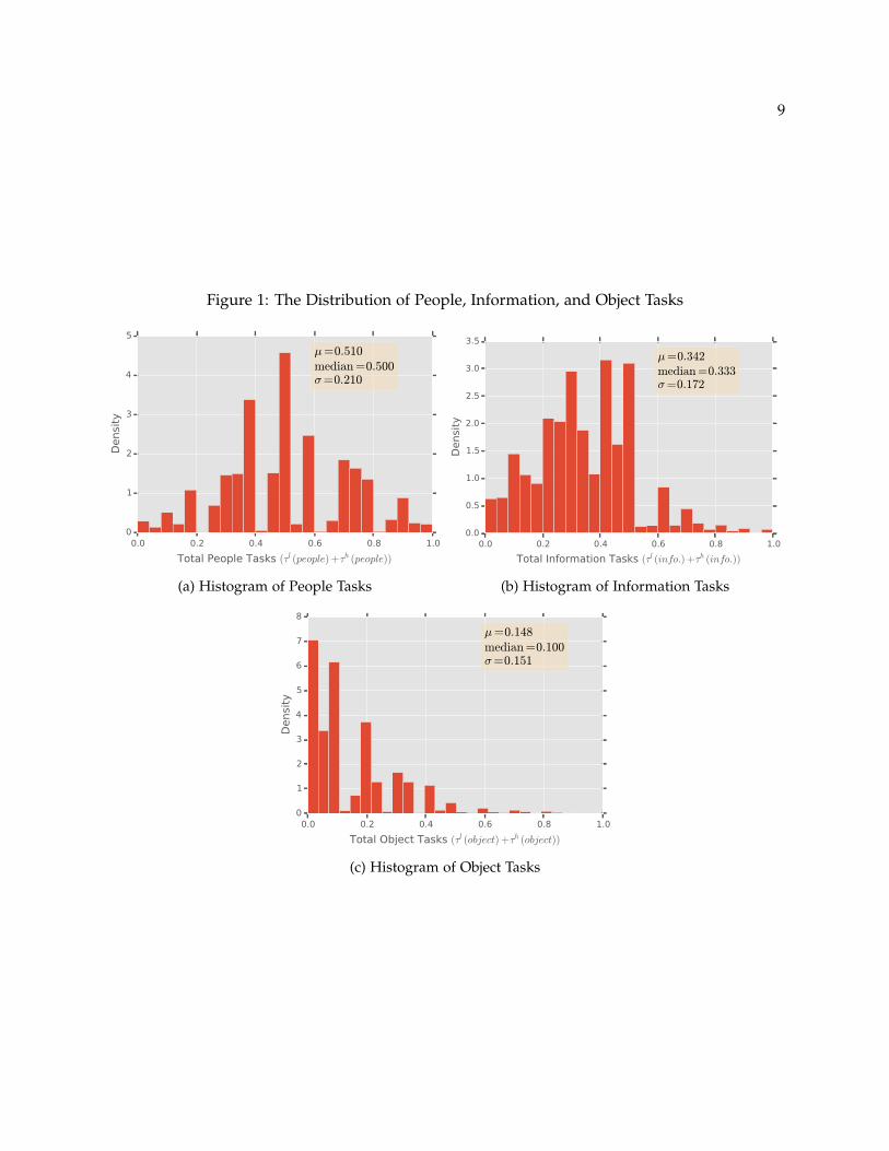
Figure 1: The Distribution of People, Information, and Object Tasks

0.0 0.2 0.4 0.6 0.8 1.0

Total People Tasks (τl (people) +τh (people))

0

1

2

3

4

5

Densi

ty

µ=0.510median =0.500σ=0.210

(a) Histogram of People Tasks

0.0 0.2 0.4 0.6 0.8 1.0

Total Information Tasks (τl (info.) +τh (info.))

0.0

0.5

1.0

1.5

2.0

2.5

3.0

3.5

Densi

ty

µ=0.342median =0.333σ=0.172

(b) Histogram of Information Tasks

0.0 0.2 0.4 0.6 0.8 1.0

Total Object Tasks (τl (object) +τh (object))

0

1

2

3

4

5

6

7

8

Densi

ty

µ=0.148median =0.100σ=0.151

(c) Histogram of Object Tasks

3.1 The Distribution of Job Tasks

In this section we present results pooling data over the ten year longitudinal sample. We begin

by examining the distribution of the amount of time that workers spend performing people,

information, and object tasks, for the moment abstracting away from the distinction between

high and low skilled tasks. Figure 1 shows the density function of τl(k) + τh(k) for each of the

three task categories k. The unit of measurement for the horizontal axes in these figures is the

fraction of time spent performing each task.8 Figure 1 shows that, on average, workers spend 51

percent of their time on people tasks, mean(τl(P) + τh(P)

)= 0.51, 34 percent of their time on

information tasks, and only 15 percent of their time on object tasks. The standard deviations of

tasks indicate that there is significant variation across jobs in the fraction of time spent performing

each task, with people tasks varying the most (σ = 0.21), object tasks varying the least (σ = 0.15),

and information tasks lying in between the two extremes.

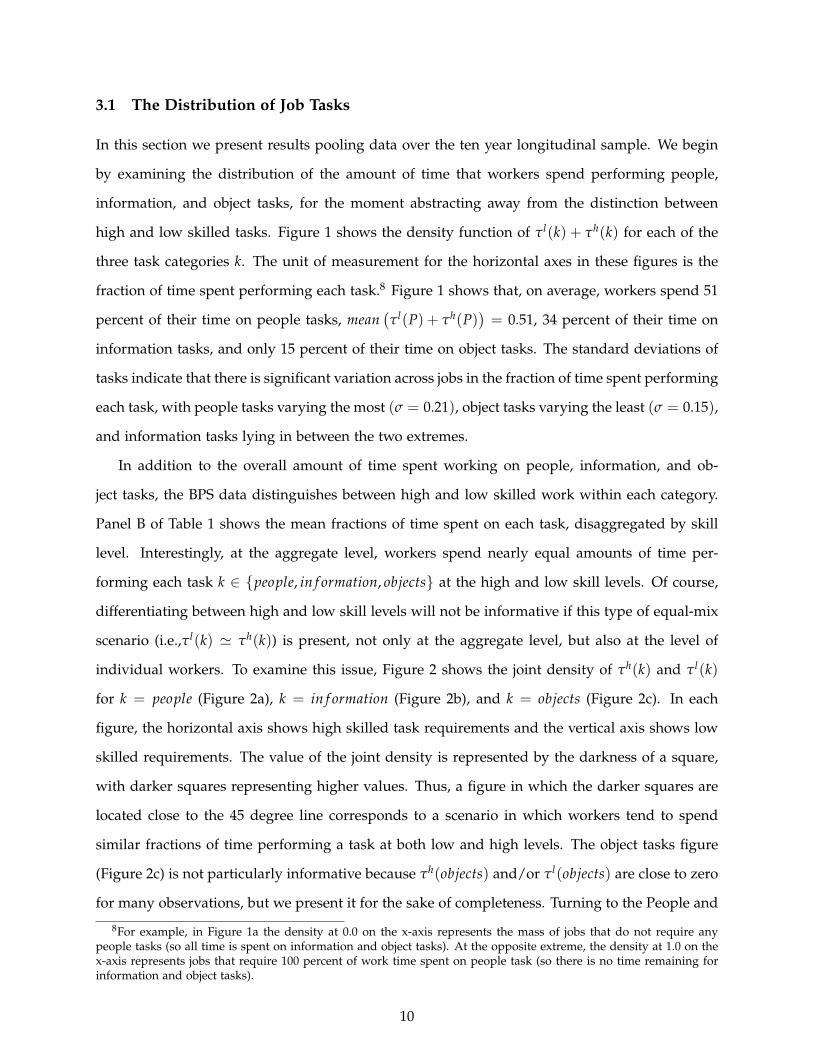
In addition to the overall amount of time spent working on people, information, and ob-

ject tasks, the BPS data distinguishes between high and low skilled work within each category.

Panel B of Table 1 shows the mean fractions of time spent on each task, disaggregated by skill

level. Interestingly, at the aggregate level, workers spend nearly equal amounts of time per-

forming each task k ∈ {people, in f ormation, objects} at the high and low skill levels. Of course,

differentiating between high and low skill levels will not be informative if this type of equal-mix

scenario (i.e.,τl(k) ' τh(k)) is present, not only at the aggregate level, but also at the level of

individual workers. To examine this issue, Figure 2 shows the joint density of τh(k) and τl(k)

for k = people (Figure 2a), k = in f ormation (Figure 2b), and k = objects (Figure 2c). In each

figure, the horizontal axis shows high skilled task requirements and the vertical axis shows low

skilled requirements. The value of the joint density is represented by the darkness of a square,

with darker squares representing higher values. Thus, a figure in which the darker squares are

located close to the 45 degree line corresponds to a scenario in which workers tend to spend

similar fractions of time performing a task at both low and high levels. The object tasks figure

(Figure 2c) is not particularly informative because τh(objects) and/or τl(objects) are close to zero

for many observations, but we present it for the sake of completeness. Turning to the People and

8For example, in Figure 1a the density at 0.0 on the x-axis represents the mass of jobs that do not require anypeople tasks (so all time is spent on information and object tasks). At the opposite extreme, the density at 1.0 on thex-axis represents jobs that require 100 percent of work time spent on people task (so there is no time remaining forinformation and object tasks).

10

11

Figure 2: The Joint Distribution of High and Low Skilled Tasks

0.0 0.2 0.4 0.6 0.8 1.0

High Skilled People (τh (people))

0.0

0.2

0.4

0.6

0.8

1.0

Low

Ski

lled P

eople

(τl

(people

))

1σ

0.000

0.005

0.010

0.015

0.020

0.025

0.030

0.035

0.040

0.045

Fract

ion

(a) People Tasks

0.0 0.2 0.4 0.6 0.8 1.0

High Skilled Information (τh (info.))

0.0

0.2

0.4

0.6

0.8

1.0

Low

Ski

lled Info

rmati

on (τl

(info.)

)

1σ

0.000

0.008

0.016

0.024

0.032

0.040

0.048

0.056

0.064

0.072

Fract

ion

(b) Information Tasks

0.0 0.2 0.4 0.6 0.8 1.0

High Skilled Object (τh (object))

0.0

0.2

0.4

0.6

0.8

1.0

Low

Ski

lled O

bje

ct (τl

(object)

)

1σ

0.00

0.05

0.10

0.15

0.20

0.25

0.30

0.35

0.40

Fract

ion

(c) Object Tasks

Information figures, the equal-mix scenario is more evident for information tasks (Figure 2b).9

However, for both k = people and k = in f ormation, individuals often spend somewhat uneven

fractions of time performing tasks at high and low levels.

If we had found that each worker tends to spend a very similar fraction of time performing

task k at a high level and task k at a low level. then the distributions of τh(k) and τl(k) would

have similar shapes as the distributions of τl(k) + τh(k) in Figure 1. Further, under this scenario,

the support of the distributions ofτh(k) and τl(k) would be compressed to the [0,.5] interval and

the standard deviations of τh(k) and τl(k) would be half as large as the standard deviations

of τl(k) + τh(k). The distributions of τh(k) and τl(k), k = people,k = in f ormation, and k =

objects are shown in Figure 3. As expected given our finding that the equal-mix scenario is

less prominent for k = people than for k = in f ormation, the standard deviations fall by less for

k = people (from .210 in 1a to .176 and .190 in 3a and 3b, respectively) than for k = in f ormation

(from .172 in 1b to .125 and .126 in 3c and 3d, respectively). However, because the majority of

people do not satisfy the equal-mix scenario for k = people and k = in f ormation, the standard

deviations of τh(k) and τl(k) remain substantially greater than half of the standard deviation of

τl(k) + τh(k). Generally speaking, for any k, a non-trivial number of people end up with close

to zero time performing k at a high skilled level and a non-trivial number of people end up with

very little time performing k at a low skilled level. However, Figure 2a shows that it is difficult

to avoid performing at least some low-skilled people tasks.

3.2 Task-Specific Work Experience Over the Career

Up to this point, the descriptive analysis of job tasks has pooled all data over the ten year longi-

tudinal sample. This section focuses on using the panel aspect of the data to discover new facts

about how workers spend their time on-the-job over their careers. Specifically, we now turn to

a description of the distribution of task-specific work experience.

Using the unique features of our panel data, we are able to compute the first measures de-

scribing the cumulative amount of time that individuals have spent on different tasks over their

career. These proxies for human capital incorporate the task variables, which are measured in

fraction of time units, along with data on the hours worked by each worker. Specifically, the

9The percentage of jobs located along the 45 degree line for people and information tasks are 21% and 35%,respectively

12

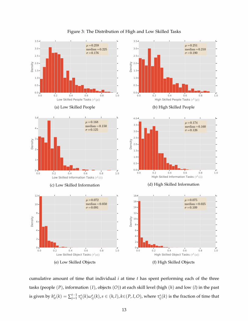
Figure 3: The Distribution of High and Low Skilled Tasks

0.0 0.2 0.4 0.6 0.8 1.0

Low Skilled People Tasks (τl (p))

0.0

0.5

1.0

1.5

2.0

2.5

3.0

3.5

Densi

ty

µ=0.259median =0.225σ=0.176

(a) Low Skilled People

0.0 0.2 0.4 0.6 0.8 1.0

High Skilled People Tasks (τh (p))

0.0

0.5

1.0

1.5

2.0

2.5

3.0

3.5

Densi

ty

µ=0.251median =0.210σ=0.190

(b) High Skilled People

0.0 0.2 0.4 0.6 0.8 1.0

Low Skilled Information Tasks (τl (i))

0

1

2

3

4

5

Densi

ty

µ=0.168median =0.150σ=0.125

(c) Low Skilled Information

0.0 0.2 0.4 0.6 0.8 1.0

High Skilled Information Tasks (τh (i))

0.0

0.5

1.0

1.5

2.0

2.5

3.0

3.5

4.0

Densi

ty

µ=0.174median =0.160σ=0.126

(d) High Skilled Information

0.0 0.2 0.4 0.6 0.8 1.0

Low Skilled Object Tasks (τl (o))

0

2

4

6

8

10

12

Densi

ty

µ=0.072median =0.050σ=0.091

(e) Low Skilled Objects

0.0 0.2 0.4 0.6 0.8 1.0

High Skilled Object Tasks (τh (o))

0

2

4

6

8

10

12

14

16

18

Densi

ty

µ=0.075median =0.025σ=0.109

(f) High Skilled Objects

cumulative amount of time that individual i at time t has spent performing each of the three

tasks (people (P), information (I), objects (O)) at each skill level (high (h) and low (l) in the past

is given by hsit(k) = ∑t−1

j=1 τsij(k)ω

sij(k), s ∈ (h, l), k∈(P, I, O), where τs

ij(k) is the fraction of time that

13

individual i spends performing task k at skill level s in time j and ωsij(k) is a weight derived from

the hours that person i works in time t. The hours weight is ωsij(k) = hoursij/40, where hoursij

represents the hours worked by worker i on his job at time j. The weights are normalized in this

manner so that ωsij(k) = 1 indicates that a worker works a forty hour week. We make use of

the hours data based on the premise that the amount of learning-by-doing depends on the time

allocated to each task, rather than simply the percentage of time spent on each task.10

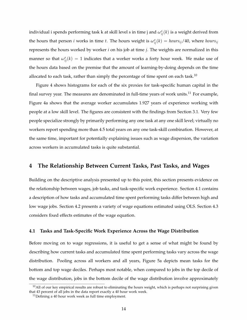
Figure 4 shows histograms for each of the six proxies for task-specific human capital in the

final survey year. The measures are denominated in full-time years of work units.11 For example,

Figure 4a shows that the average worker accumulates 1.927 years of experience working with

people at a low skill level. The figures are consistent with the findings from Section 3.1. Very few

people specialize strongly by primarily performing any one task at any one skill level; virtually no

workers report spending more than 4.5 total years on any one task-skill combination. However, at

the same time, important for potentially explaining issues such as wage dispersion, the variation

across workers in accumulated tasks is quite substantial.

4 The Relationship Between Current Tasks, Past Tasks, and Wages

Building on the descriptive analysis presented up to this point, this section presents evidence on

the relationship between wages, job tasks, and task-specific work experience. Section 4.1 contains

a description of how tasks and accumulated time spent performing tasks differ between high and

low wage jobs. Section 4.2 presents a variety of wage equations estimated using OLS. Section 4.3

considers fixed effects estimates of the wage equation.

4.1 Tasks and Task-Specific Work Experience Across the Wage Distribution

Before moving on to wage regressions, it is useful to get a sense of what might be found by

describing how current tasks and accumulated time spent performing tasks vary across the wage

distribution. Pooling across all workers and all years, Figure 5a depicts mean tasks for the

bottom and top wage deciles. Perhaps most notable, when compared to jobs in the top decile of

the wage distribution, jobs in the bottom decile of the wage distribution involve approximately

10All of our key empirical results are robust to eliminating the hours weight, which is perhaps not surprising giventhat 43 percent of all jobs in the data report exactly a 40 hour work week.

11Defining a 40 hour work week as full time employment.

14

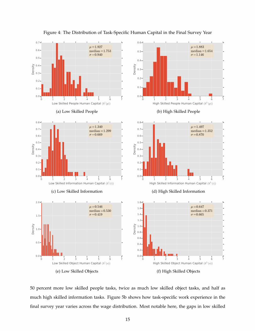
Figure 4: The Distribution of Task-Specific Human Capital in the Final Survey Year

0 1 2 3 4 5 6 7

Low Skilled People Human Capital (hl (p))

0.0

0.1

0.2

0.3

0.4

0.5

0.6

0.7

Densi

ty

µ=1.927median =1.753σ=0.940

(a) Low Skilled People

0 1 2 3 4 5 6 7

High Skilled People Human Capital (hh (p))

0.0

0.1

0.2

0.3

0.4

0.5

0.6

Densi

ty

µ=1.883median =1.654σ=1.146

(b) High Skilled People

0 1 2 3 4 5 6 7

Low Skilled Information Human Capital (hl (i))

0.0

0.1

0.2

0.3

0.4

0.5

0.6

0.7

0.8

Densi

ty

µ=1.340median =1.299σ=0.669

(c) Low Skilled Information

0 1 2 3 4 5 6 7

High Skilled Information Human Capital (hh (i))

0.0

0.1

0.2

0.3

0.4

0.5

0.6

0.7

0.8

Densi

ty

µ=1.497median =1.352σ=0.870

(d) High Skilled Information

0 1 2 3 4 5 6 7

Low Skilled Object Human Capital (hl (o))

0.0

0.5

1.0

1.5

2.0

Densi

ty

µ=0.546median =0.530σ=0.419

(e) Low Skilled Objects

0 1 2 3 4 5 6 7

High Skilled Object Human Capital (hh (o))

0.0

0.2

0.4

0.6

0.8

1.0

1.2

1.4

1.6

1.8

Densi

ty

µ=0.647median =0.371σ=0.665

(f) High Skilled Objects

50 percent more low skilled people tasks, twice as much low skilled object tasks, and half as

much high skilled information tasks. Figure 5b shows how task-specific work experience in the

final survey year varies across the wage distribution. Most notable here, the gaps in low skilled

15

Figure 5: Tasks and Human Capital by Wage Decile

τl (p) τh (p) τl (i) τh (i) τl (o) τh (o)

Tasks by Wage Decile

0.0

0.1

0.2

0.3

0.4

0.5

Mean F

ract

ion o

f Tim

e

Bottom Wage Decile

Top Wage Decile

(a) Tasks by Wage Decile

hl (p) hh (p) hl (i) hh (i) hl (o) hh (o)

Human Capital by Wage Decile (Final Survey Year)

0.0

0.5

1.0

1.5

2.0

2.5

3.0

3.5

Mean P

ers

on-Y

ears

Acc

um

ula

ted Bottom Wage Decile

Top Wage Decile

(b) Human Capital by Wage Decile

task usage that were seen between the bottom and top wage deciles in Figure 5a have either

narrowed (people) or disappeared altogether (objects). On the other hand, the largest gap that

was observed for high skilled task usage (information) in Figure 5a remains at least as large as

before and a new gap has emerged for high skilled objects tasks. Thus, our descriptive results in

5a and 5b suggest that both current and past tasks may play an important role in determining

wages, with high skill past tasks potentially being more important than low skill past tasks.

4.2 OLS Wage Equation Estimates

The large majority of the human capital literature has focused on human capital produced during

the formal schooling period. In recognition of a central assumption in this literature - that

observable academic measures are reasonably viewed as direct measures of human capital at

the time of entrance to the workforce - column 1 of Table 2 shows a regression of log-wages on

college GPA and demographic characteristics. The coefficient on GPA is quantitatively large and

statistically significant (t-stat of approximately 6). Nonetheless, the fact that the R2 in column 1 is

only 0.014 reinforces the message in much prior research that understanding how human capital

accumulates in the post-schooling period is of great importance for understanding the evolution

of earnings (Ben-Porath, 1967; Mincer, 1974; Katz and Murphy, 1992; Heckman, Lochner, and

Taber, 1998).

Unfortunately, in the post-schooling period, it is typically not possible to observe either in-

puts into the production of human capital or any direct measures of human capital (Bowlus and

16

Robinson, 2012). In practice, empirical researchers attempt to proxy for a worker’s human capi-

tal using observable characteristics that are related to wages, with experience measures (overall

experience or experience in different occupations) playing a prominent role given their time-

varying nature. However, the potential incompleteness of experience measures can be seen in

our application. For our sample of educated workers, the employment rate of 87 percent shown

in Table 1 implies that there is relatively little variation in overall work experience. In addition,

the majority of our sample of college educated workers would be expected to obtain experience

primarily in white collar occupations. Thus, a measure of overall experience (or separate experi-

ence measures for Blue Collar and White Collar occupations) may be unlikely to capture much of

the variation in the types of work experience that people accumulate during their careers. Some

evidence of this is seen in column 2 of Table 2 which adds an overall experience measure to the

wage regression. While the experience variable is significant and the new R2 is approximately

3.5 times as large as before (column 1), the R2 remains less than 0.06.12

The six measures hsit(k), s ∈ (h, l), k∈(P, I, O) described in Section 3.2 allow a more complete

and in-depth way to characterize the activities that a person has performed during his career.

Column 6 of Table 2 adds these six measures to the wage regression along with the five measures

that characterize the tasks a person is currently performing on the job. The task parameters

in the wage equation are measured relative to the omitted task category of low skilled object

tasks, τl(O).13 Confirming that the new variables constructed from our time allocation measures

contain substantial content, the R2 of the regression that includes the new measures is 0.112

(column 6). Thus, the new measures explain ten times more of the variation in wages than the

individual characteristics (column 1, R2 = 0.014) and the increase in the R2 from adding these

measures is over two times larger than the increase from adding only the standard experience

measure (column 2).

Note that an appealing and unique aspect of both the τs(k) measures and the hs(k) measures

is that they have have very clear interpretations. For example, τl(P) = 0.20 means that a person

spends 20 percent of his time in year t performing people tasks at a low skill level. Similarly,

12The R2 measures in these regressions may seem small relative to those reported by many other studies. However,it is important to keep in mind that our sample consists of individuals who graduated from a single college.

13There are only five task measures included in the regression because by definition the six “fraction of time” taskmeasures must sum to one for each job.

17

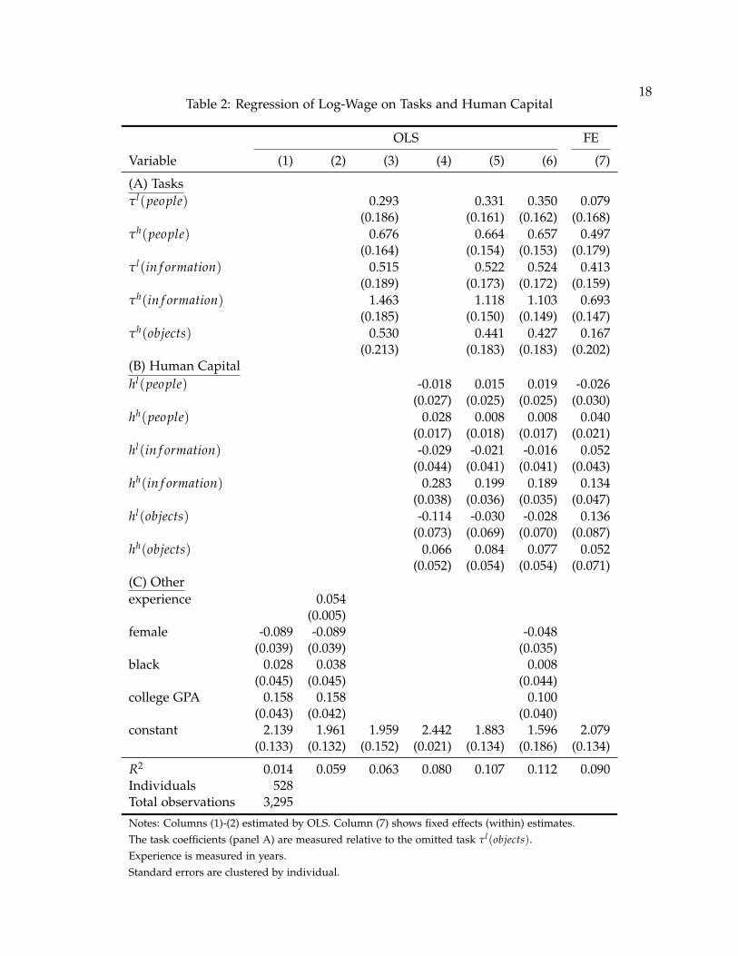
18Table 2: Regression of Log-Wage on Tasks and Human Capital

OLS FE

Variable (1) (2) (3) (4) (5) (6) (7)

(A) Tasksτl(people) 0.293 0.331 0.350 0.079

(0.186) (0.161) (0.162) (0.168)τh(people) 0.676 0.664 0.657 0.497

(0.164) (0.154) (0.153) (0.179)τl(in f ormation) 0.515 0.522 0.524 0.413

(0.189) (0.173) (0.172) (0.159)τh(in f ormation) 1.463 1.118 1.103 0.693

(0.185) (0.150) (0.149) (0.147)τh(objects) 0.530 0.441 0.427 0.167

(0.213) (0.183) (0.183) (0.202)(B) Human Capitalhl(people) -0.018 0.015 0.019 -0.026

(0.027) (0.025) (0.025) (0.030)hh(people) 0.028 0.008 0.008 0.040

(0.017) (0.018) (0.017) (0.021)hl(in f ormation) -0.029 -0.021 -0.016 0.052

(0.044) (0.041) (0.041) (0.043)hh(in f ormation) 0.283 0.199 0.189 0.134

(0.038) (0.036) (0.035) (0.047)hl(objects) -0.114 -0.030 -0.028 0.136

(0.073) (0.069) (0.070) (0.087)hh(objects) 0.066 0.084 0.077 0.052

(0.052) (0.054) (0.054) (0.071)(C) Otherexperience 0.054

(0.005)female -0.089 -0.089 -0.048

(0.039) (0.039) (0.035)black 0.028 0.038 0.008

(0.045) (0.045) (0.044)college GPA 0.158 0.158 0.100

(0.043) (0.042) (0.040)constant 2.139 1.961 1.959 2.442 1.883 1.596 2.079

(0.133) (0.132) (0.152) (0.021) (0.134) (0.186) (0.134)

R2 0.014 0.059 0.063 0.080 0.107 0.112 0.090Individuals 528Total observations 3,295

Notes: Columns (1)-(2) estimated by OLS. Column (7) shows fixed effects (within) estimates.The task coefficients (panel A) are measured relative to the omitted task τl(objects).Experience is measured in years.Standard errors are clustered by individual.

hh(I) = 1.5 means that a person has spent a total of 1.5 years in the past performing high skilled

information tasks.

The estimates related to current tasks shown in column 6 of Table 2 make considerable in-

tuitive sense, with two main takeaways. First, performing object tasks has particularly negative

implications for wages, especially if these tasks are performed at a low skill level. Second,

performing tasks at high skill levels rather than low skill levels is associated with large wage

increases. To see the quantitative importance of these facts, consider a person who is spending

at least half of his current hours working in low skilled objects tasks (i.e, τl(O) > 0.50). With

respect to the wage penalty for low skilled object tasks, holding constant the person’s past work,

moving half of her current work hours from low skilled objects tasks to low skilled people tasks

is associated with an increase in earnings of 17.5 percent (0.350/2× 100%). With respect to the

large payoff for high skilled work, moving half of her current work hours from low skilled objects

tasks to high skilled people tasks (instead of low skilled people tasks) leads to an almost dou-

bling of this wage increase to 32.8 percent (0.657/2× 100%). Similarly, moving half of her current

work hours from low skilled objects tasks to low skilled information tasks is associated with an

increase in earnings of 26 percent (0.524/2× 100%), and moving half of her current work hours

from low skilled objects tasks to high skilled information tasks (instead of low skilled informa-

tion tasks) leads to a more than doubling of this wage increase to 55 percent (1.103/2× 100%).

As some final evidence of the wage premium for high skilled tasks, moving half of her current

work from low skilled objects tasks to high skilled objects tasks leads to an increase in wages of

21 percent (0.427/2× 100%).

Turning to the six proxies for task-specific human capital, hs(k), s ∈ (h, l), k∈(P, I, O), that

describe a person’s past activities, perhaps most striking in column 6 of Table 2 is the role of

accumulated time spent performing high skilled information tasks. The estimated coefficient on

hh(I) of 0.189 indicates that a worker with one extra person-year of experience performing high

skilled information tasks earns 18.9 percent more than a worker with no such work experience,

and the associated t-statistic is 5.4. The estimated coefficient on hh(O) of 0.077 is also quantita-

tively large, although neither this estimated effect or the estimated effect of hh(P) is significant at

conventional levels (t-statistics of 1.42 and .47, respectively). In contrast, there is no evidence that

the amount of time spent performing tasks at low skill levels in the past has any relationship with

19

current wages. The point estimates associated with the three low skilled tasks are economically

quite small (hl(P) = 0.019, hl(I) = −0.016, and hlt(O) = −0.028) and the associated t-statistics

are are each below 1.0.

Thus, the results suggest that working in high skilled information tasks is important for

creating one’s human capital. We note, however, that this interpretation requires a causal inter-

pretation of the estimated effects of hst(k), s ∈ (h, l), k∈(P, I, O). A general issue that arises in

the interpretation of an observed relationship between tasks and wages is that there may exist

a correlation between unobserved worker ability and job tasks. For example, it may be the case

that high ability workers tend to work in high skilled jobs. The results in the first six columns of

Table 2 could be viewed as causal if conditioning on observed individual characteristics removed

any correlation that was present. It is worth noting that our study of one school is perhaps

desirable in this respect both because it removes the possibility that a correlation exists because

of unobserved school quality and because it allows us to use a measure of ability, one’s college

GPA, that is directly comparable across workers. Nonetheless, given that column 1 of Table 2

found that our standard conditioning variables explain only 1.4 percent of the variation in log

earnings, it is natural to be concerned that some correlation may remain. In the next section,

we take advantage of our ability to exploit within-person variation in present and past tasks to

examine this issue further.

4.3 Fixed Effects Wage Equation Estimates

A major advantage of having access to longitudinal data is that we can estimate the model by

Fixed Effects to control for permanent, unobserved differences across workers that could be

correlated with job tasks. For the use of this estimator it is crucial that our tasks are measured

at the level of individual jobs. As discussed earlier, when tasks are not measured at the level

of individual jobs, researchers typically assign all workers in a particular occupation the same

tasks from the DOT or O*NET. However, in this scenario, changes in tasks will not be useful for

explaining any of the substantial changes in earnings that are known to exist for a person within

an occupation. Further, our time allocation measures are also important in this context because it

is not obvious how to best difference task usage information that is characterized in a qualitative

manner (important, very important, etc.).

20

Column 7 of Table 2 shows Fixed Effects (within) estimates of the log-wage equation.14 Be-

ginning with the current task information, a 37 percent decrease in the coefficient on τh(I) is

observed as we move from OLS (Column 6) to fixed effects (Column 7). This decrease is consis-

tent with the hypothesis that the OLS estimator is upward biased due to a positive correlation

between unobserved worker ability and the tendency to perform high skilled information tasks.

Nonetheless, the estimated wage effect of working in a job with high skilled information tasks

remains quantitatively large and statistically significant. The estimated coefficient on τh(I) of

0.693 is the largest of the five task coefficients and the associated t-statistic is greater than 2.5.

Similarly, the fixed effects estimated coefficients on τh(P) and τl(I) are 24 percent and 21 percent

smaller than the OLS estimates, but still indicate economically large and statistically significant

wage premia for performing high skilled people tasks and low skilled information tasks relative

to low skilled object tasks (point estimates of .497 for τh(P) and .413 for τl(I), and p-values of

0.006 and 0.010). Perhaps the biggest differences between the fixed effects and OLS results are

seen in the remaining two variables, with both the coefficient on τl(P) and the coefficient on

τh(O) falling by over 50 percent. Nonetheless, overall, the general takeaway from the current

tasks results is similar to that found using OLS, despite the fact that the fixed effect estimates are

based solely on within-person variation in tasks and wages.

The spirit of our results on the importance of task-specific human capital is also remark-

ably robust to controlling for fixed effects. Similar to what was seen with τh(I), a decrease of

30% in the estimated coefficient on n hh(I) is observed as we move from OLS to Fixed Effects.

Nonetheless, the estimated effect of accumulating experience in high skilled information tasks

remains quantitatively and statistically important, with one person-year of hh(I) being estimated

to increase wages by approximately 13 percent and the associated t-statistic having a value of

2.85. The fixed effects estimates also reveal that accumulating time in high skilled people tasks

increases future wages, with hh(P) having an estimated effect of 0.04 and a p-value of 0.059. Also

similar in spirit to the OLS results, none of the estimated low skill human capital coefficients are

statistically different from zero at conventional levels, although the point estimate for hl(O) is

quite large but imprecisely estimated. Thus, the fixed effects estimates support the intuitively ap-

pealing notion that there is considerable scope for workers to become more productive through

14The background variables in Panel (C) are not included in the fixed effects model because they are constant overtime.

21

learning as they perform high skilled tasks, with accumulated experience in high skilled infor-

mation tasks being particularly important. However, there is little evidence that performing low

skilled tasks today is a path to higher future wages.

22

23

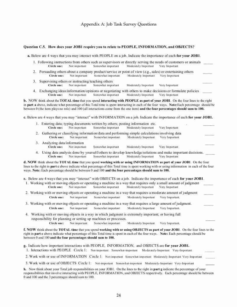
Appendix A: Job Task Survey Questions

24

References

Acemoglu, D. and D. Autor (2011). Skills, tasks and technologies: Implications for employmentand earnings. Handbook of labor economics 4, 1043–1171.

Autor, D. H. and D. Dorn (2013). The Growth of Low-Skill Service Jobs and the Polarization ofthe US Labor Market. American Economic Review 103(5), 1553–1597.

Autor, D. H. and M. J. Handel (2013). Putting Tasks to the Test: Human Capital, Job Tasks, andWages. Journal of Labor Economics 31(2), S59–S95.

Becker, G. S. (1964). Human capital theory. Columbia, New York.

Ben-Porath, Y. (1967). The Production of Human Capital and the Life Cycle of Earnings. TheJournal of Political Economy 75(4), 352 – 365.

Bowlus, A. J. and C. Robinson (2012). Human capital prices, productivity, and growth. TheAmerican Economic Review, 3483–3515.

Gathmann, C. and U. Schönberg (2010). How general is human capital? a task-based approach.Journal of Labor Economics 28(1), 1–49.

Gibbons, R. and L. Katz (1992). Does unmeasured ability explain inter-industry wage differen-tials? The Review of Economic Studies 59(3), 515–535.

Heckman, J. J., L. Lochner, and C. Taber (1998). Explaining rising wage inequality: Explorationswith a dynamic general equilibrium model of labor earnings with heterogeneous agents. Re-view of economic dynamics 1(1), 1–58.

Heckman, J. J. and G. Sedlacek (1985). Heterogeneity, aggregation, and market wage functions:an empirical model of self-selection in the labor market. The journal of political economy, 1077–1125.

Kambourov, G. and I. Manovskii (2009). Occupational specificity of human capital*. InternationalEconomic Review 50(1), 63–115.

Katz, L. F. and K. M. Murphy (1992). Changes in Relative Wages, 1963-1987: Supply and DemandFactors. Source: The Quarterly Journal of Economics 107(1), 35–78.

Manning, A. (2003). Monopsony in motion: Imperfect competition in labor markets. Princeton Univer-sity Press.

Mincer, J. (1974). Schooling, Experience, and Earnings. NBER.

Neal, D. (1995). Industry-specific human capital: Evidence from displaced workers. Journal oflabor Economics, 653–677.

25

Parent, D. (2000). Industry-specific capital and the wage profile: Evidence from the nationallongitudinal survey of youth and the panel study of income dynamics. Journal of Labor Eco-nomics 18(2), 306–323.

Poletaev, M. and C. Robinson (2008). Human capital specificity: evidence from the dictionary ofoccupational titles and displaced worker surveys, 1984–2000. Journal of Labor Economics 26(3),387–420.

Robinson, C. (2011). Occupational mobility, occupation distance and specific human capital.Technical report, CIBC Working Paper.

Sanders, C. (2014). Skill Accumulation , Skill Uncertainty , and Occupational Choice. WorkingPaper, 1–44.

Stinebrickner, R. and T. Stinebrickner (2013). A major in science? initial beliefs and final outcomesfor college major and dropout. The Review of Economic Studies, rdt025.

Stinebrickner, R. and T. R. Stinebrickner (2003). Working during school and academic perfor-mance. Journal of Labor Economics 21(2), 473–491.

Stinebrickner, R. and T. R. Stinebrickner (2006). What can be learned about peer effects usingcollege roommates? evidence from new survey data and students from disadvantaged back-grounds. Journal of public Economics 90(8), 1435–1454.

Stinebrickner, T. and R. Stinebrickner (2012). Learning about Academic Ability and the CollegeDropout Decision. Journal of Labor Economics 30, 707–748.

Sullivan, P. (2010, jun). Empirical Evidence on Occupation and Industry Specific Human Capital.Labour economics 17(3), 567–580.

Yamaguchi, S. (2010). Job Search, Bargaining, and Wage Dynamics. Journal of Labor Eco-nomics 28(3), 595–631.

26