Embed Size (px)
Citation preview

paper 43
LIFE-PATHS INTO YOUNG ADULTHOOD AND THE COURSE OF SUBSTANCE USE AND WELL-BEING:
INTER- AND INTRA-COHORT COMPARISONS
John SchulenbergPatrick M. O'Malley Jerald G. BachmanLloyd D. Johnston

LIFE-PATHS INTO YOUNG ADULTHOOD AND THE COURSE OF SUBSTANCE USE AND WELL-BEING:
INTER- AND INTRA-COHORT COMPARISONS
Monitoring the Future Occasional Paper No. 43
John SchulenbergPatrick M. O'MalleyJerald G. Bachman Lloyd D. Johnston
Institute for Social ResearchThe University of Michigan
1998

TABLE OF CONTENTS
page
LIST OF TABLES . . . . . . . . . . . . . . . . . . . . . . . . . . . . . . . . . . . . . . . . . . . . . . . . . . . . . . . . . . . . v
LIST OF FIGURES . . . . . . . . . . . . . . . . . . . . . . . . . . . . . . . . . . . . . . . . . . . . . . . . . . . . . . . . . . vi
INTRODUCTION . . . . . . . . . . . . . . . . . . . . . . . . . . . . . . . . . . . . . . . . . . . . . . . . . . . . . . . . . . . . 1
Life Paths into Young Adulthood and Health and Well-being . . . . . . . . . . . . . . . . . . . . . 1A Needed Focus on Inter- and Intra-cohort Differences and Similarities . . . . . . . . . . . . . 2
METHOD . . . . . . . . . . . . . . . . . . . . . . . . . . . . . . . . . . . . . . . . . . . . . . . . . . . . . . . . . . . . . . . . . . . 4
Sample . . . . . . . . . . . . . . . . . . . . . . . . . . . . . . . . . . . . . . . . . . . . . . . . . . . . . . . . . . . . . . . . 4Sub-sample Groups . . . . . . . . . . . . . . . . . . . . . . . . . . . . . . . . . . . . . . . . . . . . . . . . . . . . . . 5
Cohort groups . . . . . . . . . . . . . . . . . . . . . . . . . . . . . . . . . . . . . . . . . . . . . . . . . . . . . 5Life-path groups . . . . . . . . . . . . . . . . . . . . . . . . . . . . . . . . . . . . . . . . . . . . . . . . . . . 5
Measures . . . . . . . . . . . . . . . . . . . . . . . . . . . . . . . . . . . . . . . . . . . . . . . . . . . . . . . . . . . . . . 6Well-being measures . . . . . . . . . . . . . . . . . . . . . . . . . . . . . . . . . . . . . . . . . . . . . . . 6Substance use measures . . . . . . . . . . . . . . . . . . . . . . . . . . . . . . . . . . . . . . . . . . . . . 6
Analysis Plan . . . . . . . . . . . . . . . . . . . . . . . . . . . . . . . . . . . . . . . . . . . . . . . . . . . . . . . . . . . 7Overall between-subjects effects: Cohort, gender, and life-path differences . . . . 7Within subjects effects: Differential change during the transition . . . . . . . . . . . . 7
RESULTS . . . . . . . . . . . . . . . . . . . . . . . . . . . . . . . . . . . . . . . . . . . . . . . . . . . . . . . . . . . . . . . . . . . 8
Phase 1. Course of Well-being and Substance Use in Total Sample . . . . . . . . . . . . . . . . . 8Well-being . . . . . . . . . . . . . . . . . . . . . . . . . . . . . . . . . . . . . . . . . . . . . . . . . . . . . . . 8Substance use . . . . . . . . . . . . . . . . . . . . . . . . . . . . . . . . . . . . . . . . . . . . . . . . . . . . . 8
Phase 2. Cohort Comparisons . . . . . . . . . . . . . . . . . . . . . . . . . . . . . . . . . . . . . . . . . . . . . . 9Well-being . . . . . . . . . . . . . . . . . . . . . . . . . . . . . . . . . . . . . . . . . . . . . . . . . . . . . . . 9Substance use . . . . . . . . . . . . . . . . . . . . . . . . . . . . . . . . . . . . . . . . . . . . . . . . . . . . . 9Summary . . . . . . . . . . . . . . . . . . . . . . . . . . . . . . . . . . . . . . . . . . . . . . . . . . . . . . . 10
Phase 3. Gender Comparisons . . . . . . . . . . . . . . . . . . . . . . . . . . . . . . . . . . . . . . . . . . . . . 10Well-being . . . . . . . . . . . . . . . . . . . . . . . . . . . . . . . . . . . . . . . . . . . . . . . . . . . . . . 10Substance use . . . . . . . . . . . . . . . . . . . . . . . . . . . . . . . . . . . . . . . . . . . . . . . . . . . . 11Summary . . . . . . . . . . . . . . . . . . . . . . . . . . . . . . . . . . . . . . . . . . . . . . . . . . . . . . . 11
Phase 4. Life-path Comparisons . . . . . . . . . . . . . . . . . . . . . . . . . . . . . . . . . . . . . . . . . . . 11Well-being . . . . . . . . . . . . . . . . . . . . . . . . . . . . . . . . . . . . . . . . . . . . . . . . . . . . . . 11Substance use . . . . . . . . . . . . . . . . . . . . . . . . . . . . . . . . . . . . . . . . . . . . . . . . . . . . 12Summary . . . . . . . . . . . . . . . . . . . . . . . . . . . . . . . . . . . . . . . . . . . . . . . . . . . . . . . 13
iv
TABLE OF CONTENTS (continued)
page
SUMMARY AND CONCLUSIONS . . . . . . . . . . . . . . . . . . . . . . . . . . . . . . . . . . . . . . . . . . . . 15Overall Changes in Well-being and Substance Use during the Transition
to Young Adulthood . . . . . . . . . . . . . . . . . . . . . . . . . . . . . . . . . . . . . . . . . . . . . . 15Cohort Group Differences and Similarities in the Course of Well-being
and Substance Use . . . . . . . . . . . . . . . . . . . . . . . . . . . . . . . . . . . . . . . . . . . . . . . 15Gender Differences and Similarities in the Courses of Well-being
and Substance Use . . . . . . . . . . . . . . . . . . . . . . . . . . . . . . . . . . . . . . . . . . . . . . . 16Life-path Differences in the courses of Well-being and Substance Use . . . . . . . . . . . . . 17Limitations and Future Directions . . . . . . . . . . . . . . . . . . . . . . . . . . . . . . . . . . . . . . . . . . 17Conclusions . . . . . . . . . . . . . . . . . . . . . . . . . . . . . . . . . . . . . . . . . . . . . . . . . . . . . . . . . . . 18
REFERENCES . . . . . . . . . . . . . . . . . . . . . . . . . . . . . . . . . . . . . . . . . . . . . . . . . . . . . . . . . . . . . . 21
ENDNOTES . . . . . . . . . . . . . . . . . . . . . . . . . . . . . . . . . . . . . . . . . . . . . . . . . . . . . . . . . . . . . . . . 27
TABLES . . . . . . . . . . . . . . . . . . . . . . . . . . . . . . . . . . . . . . . . . . . . . . . . . . . . . . . . . . . . . . . . . . 29
FIGURES . . . . . . . . . . . . . . . . . . . . . . . . . . . . . . . . . . . . . . . . . . . . . . . . . . . . . . . . . . . . . . . . . . 39
APPENDIX . . . . . . . . . . . . . . . . . . . . . . . . . . . . . . . . . . . . . . . . . . . . . . . . . . . . . . . . . . . . . . . . . 55

v
LIST OF TABLES
page
Table 1. Comparison of Institutional Structure to Facilitate Developmental Transition: Transition into Adolescence vs. Transition into Young Adulthood. . . . . . . . . . . . . . . . . . . . . . . . . . . . . . . . . . . . . . . . . . . . . . . . . . . . . . . 30
Table 2. Life Paths into Young Adulthood: Group Definitions and Percentages. . . . . . . . 31
Table 3. Summary of Measures. . . . . . . . . . . . . . . . . . . . . . . . . . . . . . . . . . . . . . . . . . . . . 32
Table 4. Overview of Repeated Measures ANOVAs Results for Well-Beingand Substance Use. . . . . . . . . . . . . . . . . . . . . . . . . . . . . . . . . . . . . . . . . . . . . . . . 33
Table 5. Summary of Significant Overall Cohort and Cohort by Age Effects. . . . . . . . . . 34
Table 6. Summary of Significant Overall Gender and Gender by Age Effects. . . . . . . . . 35
Table 7. Summary of Significant Overall Life Path and Life Path by Age Effects. . . . . . 36
vi
LIST OF FIGURES
page
Figure 1. Monitoring the Future Longitudinal Panels by Cohort: Senior YearClasses 1976-1992. . . . . . . . . . . . . . . . . . . . . . . . . . . . . . . . . . . . . . . . . . . . . . . . 39
Figure 2. Change in Well-Being during the Transition to Young Adulthood:Total Sample. . . . . . . . . . . . . . . . . . . . . . . . . . . . . . . . . . . . . . . . . . . . . . . . . . . . 40
Figure 3. Change in Substance Use during the Transition to Young Adulthood: Total Sample . . . . . . . . . . . . . . . . . . . . . . . . . . . . . . . . . . . . . . . . . . . . . . . . . . . 41
Figure 4. Cohort Differences in Well-Being during the Transition to Young Adulthood: Self-Efficacy and Fatalism. . . . . . . . . . . . . . . . . . . . . . . . . . . . . . . . . 42
Figure 5. Cohort Differences in Substance Use during the Transition to YoungAdulthood: 30-Day Cigarette Use and 12-Month Marijuana Use. . . . . . . . . . . . 43
Figure 6. Cohort Differences in Substance Use during the Transition to Young Adulthood: 30-Day Alcohol Use and 2-Week Binge Drinking. . . . . . . . . . . . . 44
Figure 7. Gender Differences in Well-Being during the Transition to Young Adulthood: Self-Efficacy and Social Support. . . . . . . . . . . . . . . . . . . . . . . . . . . . 45
Figure 8. Gender Differences in Substance Use during the Transition to YoungAdulthood: 30-Day Cigarette Use and 12-Month Marijuana Use. . . . . . . . . . . . 46
Figure 9. Gender Differences in Substance Use during the Transition to YoungAdulthood: 30-Day Alcohol Use and 2-Week Binge Drinking . . . . . . . . . . . . . 47
Figure 10. Life Path Differences in Well-Being during the Transition to YoungAdulthood: Satisfaction with Life. . . . . . . . . . . . . . . . . . . . . . . . . . . . . . . . . . . . . 48
Figure 11. Life Path Differences in Well-Being during the Transition to YoungAdulthood: Loneliness. . . . . . . . . . . . . . . . . . . . . . . . . . . . . . . . . . . . . . . . . . . . . 49
Figure 12. Life Path Differences in Substance Use during the Transition to Young Adulthood: 30-Day Cigarette Use. . . . . . . . . . . . . . . . . . . . . . . . . . . . . . . . . . . . . 50
Figure 13. Life Path Differences in Substance Use during the Transition to YoungAdulthood: 30-Day Alcohol Use. . . . . . . . . . . . . . . . . . . . . . . . . . . . . . . . . . . . . 51
Figure 14. Life Path Differences in Substance Use during the Transition to YoungAdulthood: 2-Week Binge Drinking . . . . . . . . . . . . . . . . . . . . . . . . . . . . . . . . . . 52
Figure 15. Life Path Differences in Substance Use during the Transition to YoungAdulthood: 12-Month Marijuana Use. . . . . . . . . . . . . . . . . . . . . . . . . . . . . . . . . . 53

vii
AUTHORS' NOTE
This is part of a larger study funded by a grant from the National Institute on Drug Abuse(DA01411). This occasional paper is an expanded version of a chapter by the same authors thatwill appear in L.J. Crockett and R.K. Silbereisen (Editors), Negotiating adolescence in times ofsocial change (New York: Cambridge University Press). It is based in part on an invitedpresentation by the first author to the International Conference on Negotiating Adolescence inTimes of Social Change: Concepts and Research, Pennsylvania State University, March 1996,sponsored by the Pennsylvania State University, USA, and the Friedrich Schiller University ofJena, Germany. We thank Lisa Crockett, Rainer Silbereisen, and an anonymous reviewer forhelpful feedback on previous drafts, as well as Joyce Buchanan, Jonathon Brenner, NicoleHitzemann, Jeanette Lim, and Katherine Wadsworth for assistance with data and textmanagement and data analysis. Address correspondence to John Schulenberg, Survey Research Center, Institute for Social Research, University of Michigan, Ann Arbor, MI 48106-1248.

1
INTRODUCTION
The period between adolescence and adulthood represents a critical developmentaltransition. Diversity in life paths becomes more clearly manifest during this transition (Sherrod,1996; Sherrod, Haggerty, & Featherman, 1993), and interindividual variability in the timing andcontent of developmental milestones increases. This increased diversity is due to the realizationof life path preferences established prior to the transition as well as to the creation of new pathsas a function of experiences during the transition. The emergence of new roles and socialcontexts provides increased opportunities for successes and failures, which in turn may set thestage for potential discontinuity in functioning and adjustment between adolescence and youngadulthood (e.g., Aseltine & Gore, 1993; Petersen, 1993; Schulenberg, Wadsworth, O'Malley,Bachman, & Johnston, 1996).
At the broader societal level, there is relatively little institutional structure to facilitate thetransition to young adulthood (Hamilton, 1990; Hurrelmann, 1990). For example, there is farless institutionally- and culturally-imposed structure on the roles, experiences, and expectationsof young people when they make the transition out of adolescence compared to when they makethe transition into adolescence (see Table 1). This relative lack of structure is undoubtedlydevelopmentally beneficial for some older adolescents as they make the transition into youngadulthood. For others, however, the lack of structure creates a developmental mismatch thatadversely influences their health and well-being (see e.g., Eccles et al., 1997; Lerner, 1982;Schulenberg, Maggs, & Hurrelmann, 1997).
Moreover, as Clausen (1991), Elder (1986), and Schuman and Scott (1989) have shown,decisions and experiences during this transition can have powerful reverberations throughout thecourse of one's adulthood (see also, e.g., Marini, 1987; Mortimer, 1991). Certainly, much ofone's "foundation" is set and many of the initial decisions regarding future plans are made priorto leaving high school. But the actual experiences of young adulthood -- the joining of intentionsand realities, the deflections of initial plans and making of new ones, the episodes of successesand failures with the various normative tasks -- set the stage for the course of one's adult life.
Life Paths into Young Adulthood and Health and Well-being
The present study was undertaken to examine the impact of these new social roles andcontexts on health and well-being between the senior year of high school (age 18) and four yearspost-high school (age 22) using multi-cohort national panel data drawn from the Monitoring theFuture study (e.g., Johnston, Bachman, & O’Malley, 1995; Bachman, Wadsworth, O'Malley,Johnston & Schulenberg, 1997). This "launching" period immediately following high school isan important one, for it is when initial plans combine with experiences to set into motion thepaths that will take the young person through the transition and into adulthood (Gore, Aseltine,Colten & Lin, 1997). We build upon previous research with the Monitoring the Future data thathas shown the importance of such experiences as marriage and living arrangements on post-highschool substance use (e.g., Bachman, O'Malley, & Johnston, 1984; Bachman et al., 1997), andtake a pattern-centered approach to focus on individual life paths defined by the combination of
Occasional Paper No. 43
2
individual's social roles and experiences during the transition. Specifically, individuals wereplaced into mutually exclusive life path groups depending on their experiences during thislaunching period.
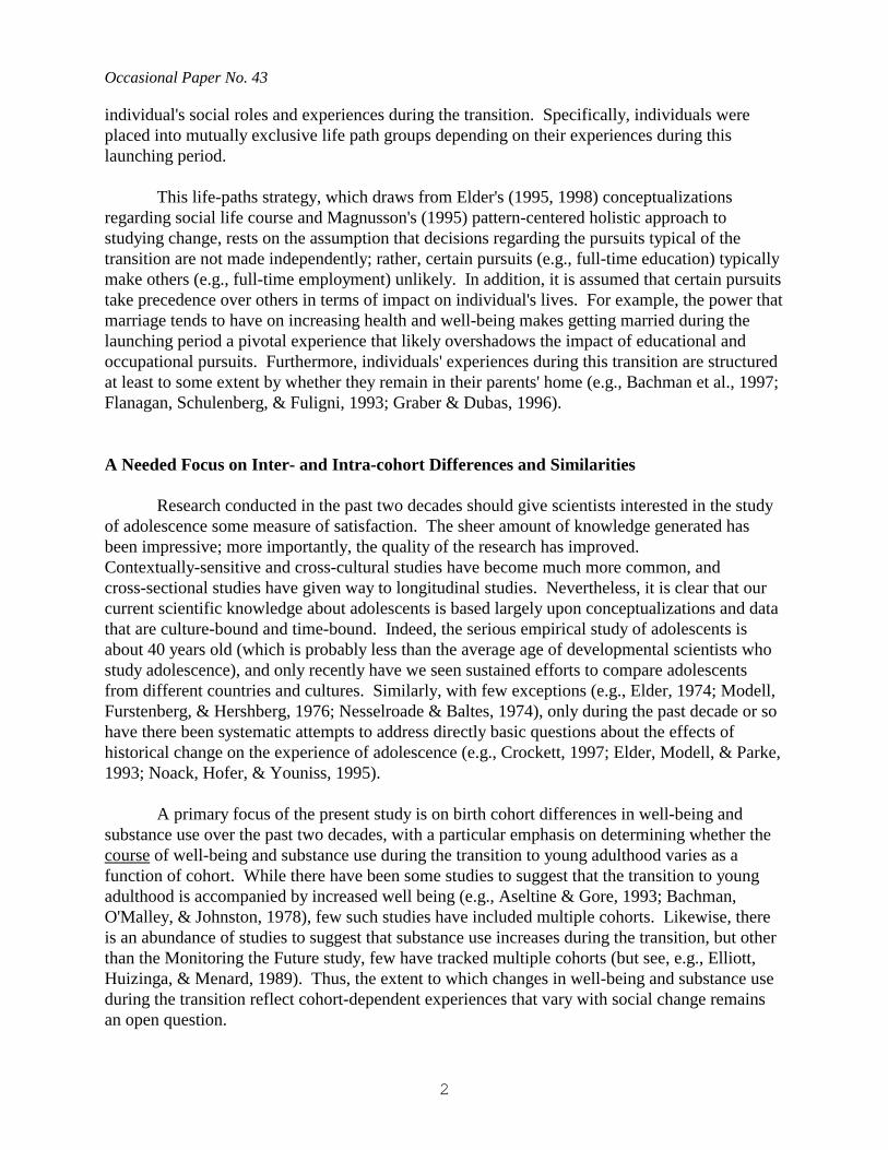
This life-paths strategy, which draws from Elder's (1995, 1998) conceptualizationsregarding social life course and Magnusson's (1995) pattern-centered holistic approach tostudying change, rests on the assumption that decisions regarding the pursuits typical of thetransition are not made independently; rather, certain pursuits (e.g., full-time education) typicallymake others (e.g., full-time employment) unlikely. In addition, it is assumed that certain pursuitstake precedence over others in terms of impact on individual's lives. For example, the power thatmarriage tends to have on increasing health and well-being makes getting married during thelaunching period a pivotal experience that likely overshadows the impact of educational andoccupational pursuits. Furthermore, individuals' experiences during this transition are structuredat least to some extent by whether they remain in their parents' home (e.g., Bachman et al., 1997;Flanagan, Schulenberg, & Fuligni, 1993; Graber & Dubas, 1996).
A Needed Focus on Inter- and Intra-cohort Differences and Similarities
Research conducted in the past two decades should give scientists interested in the studyof adolescence some measure of satisfaction. The sheer amount of knowledge generated hasbeen impressive; more importantly, the quality of the research has improved. Contextually-sensitive and cross-cultural studies have become much more common, andcross-sectional studies have given way to longitudinal studies. Nevertheless, it is clear that ourcurrent scientific knowledge about adolescents is based largely upon conceptualizations and datathat are culture-bound and time-bound. Indeed, the serious empirical study of adolescents isabout 40 years old (which is probably less than the average age of developmental scientists whostudy adolescence), and only recently have we seen sustained efforts to compare adolescentsfrom different countries and cultures. Similarly, with few exceptions (e.g., Elder, 1974; Modell,Furstenberg, & Hershberg, 1976; Nesselroade & Baltes, 1974), only during the past decade or sohave there been systematic attempts to address directly basic questions about the effects ofhistorical change on the experience of adolescence (e.g., Crockett, 1997; Elder, Modell, & Parke,1993; Noack, Hofer, & Youniss, 1995).
A primary focus of the present study is on birth cohort differences in well-being andsubstance use over the past two decades, with a particular emphasis on determining whether thecourse of well-being and substance use during the transition to young adulthood varies as afunction of cohort. While there have been some studies to suggest that the transition to youngadulthood is accompanied by increased well being (e.g., Aseltine & Gore, 1993; Bachman,O'Malley, & Johnston, 1978), few such studies have included multiple cohorts. Likewise, thereis an abundance of studies to suggest that substance use increases during the transition, but otherthan the Monitoring the Future study, few have tracked multiple cohorts (but see, e.g., Elliott,Huizinga, & Menard, 1989). Thus, the extent to which changes in well-being and substance useduring the transition reflect cohort-dependent experiences that vary with social change remainsan open question.
Life-Paths into Young Adulthood
3
In the past two decades in the United States, macrolevel social change is probably bestconceptualized as emerging fairly continuously (e.g., increased availability of personalcomputers, increased maternal employment, increased college attendance and age of firstmarriage), rather than as a function of single defining historical events (e.g., the GreatDepression). This, of course, makes it difficult to isolate social change and to capture its natureand impact. Still, in terms of "youth culture," the last two decades have witnessed someimportant macrolevel changes. For example, during the late 1970s (when Jimmy Carter waspresident), conservative and materialistic values were low and altruistic values were high; thispattern was reversed during the early and middle 1980s (when Ronald Reagan was president),and then reversed again during the early 1990s (when George Bush was president) (e.g., seeSchulenberg, Bachman, Johnston, & O'Malley, 1995). During these same three historicalperiods, there were important changes in illicit drug use among young people, with a decline inillicit drug use during the 1980s, followed by an upturn in the early 1990s (Johnston, O'Malley,& Bachman, 1998). Another important historical trend was that by the end of the 1970s, the lastbirth cohorts of the "baby-boom generation" had progressed through high school, with the post-baby boom cohorts (sometimes popularly referred to as "Generation X") experiencingadolescence during the 1980s when economic and demographic forces lead many to believe thatcareer prospects would be more limited (e.g., Holtz, 1995).
Given these macro-level social changes, and given the opportunities and constraints inour data set, we focus the present study on three cohort groups: Cohort 1 consisted of those whowere seniors in high school during the period of 1976 through 1981; Cohort 2 consisted of the1982-86 senior year cohorts; and Cohort 3 consisted of the 1987-92 senior year cohorts. It isimportant to recognize that this emphasis on cohort groups, while appropriate given our purposeshere, nevertheless serves to confound period effects (i.e., secular trends) with cohort effects andto a lesser extent with age effects.
Clearly, inter-cohort comparisons are important, but they become more important whenintra-cohort comparisons are also conducted (e.g., Ryder, 1965). Social change hardly everstrikes a cohort uniformly, and intra-cohort comparisons permit us to see how pervasive theeffects of social change may be, as well as to begin to understand the mechanisms that connecthistorical and individual change. In the present study, we focus on how cohort interacts with lifepaths and gender in influencing the course of well-being and substance use during the transitionto young adulthood.
In summary, the present study was undertaken to examine the courses of well-being andsubstance use during the transition to young adulthood. We used multi-cohort U.S. nationalpanel data spanning ages 18 to 22 to describe the courses of well-being and substance use and todetermine whether the courses varied as a function of cohort, gender, and life-paths, as well as afunction of interactions among cohort, gender, and life paths.

Occasional Paper No. 43
4
METHOD
Three waves of national panel data from 17 consecutive cohorts were obtained from theMonitoring the Future (MtF) project. MtF is an ongoing cohort-sequential longitudinal projectdesigned to understand the epidemiology and etiology of substance use and, more broadly,psychosocial development during adolescence and young adulthood. The project has surveyednationally representative samples of approximately 17,000 high school seniors each year in theUnited States since 1975, using questionnaires administered in classrooms. Approximately 2,400individuals are randomly selected from each senior year cohort for follow-up. Follow-up surveysare conducted on a biennial basis, using mailed questionnaires. Additional details regarding theMtF project procedures and purposes are provided elsewhere (Bachman, Johnston, & O'Malley,1996; Johnston et al., 1998; Johnston, O'Malley, Schulenberg, & Bachman, 1996).
Sample
The panel sample used in the present study consisted of 17 consecutive cohorts ofrespondents who were surveyed as high school seniors (Base Year or Wave 1) in 1976 through1992, and who participated in the first two biennial follow-up surveys (Follow-Ups 1 and 2, orWaves 2 and 3, respectively). The biennial follow-up surveys begin one year post-high schoolfor one random half of each cohort, and two years post-high school for the other half. Thestructure of the data set is illustrated in Figure 1. For example, as is shown, the 1976 senior yearcohort had their base year (BY) survey in 1976; for one random half of this cohort, the first andsecond follow-ups (FU1 and FU2) occurred one and three years after high school (1977 and1979), and for the other random half, FU1 and FU2 occurred two and four years after high school(1978 and 1980). For these analyses, the two random halves were combined to comprise twofollow-up surveys with FU1 covering the first and second year out of high school (modal ages19-20), and FU2 covering the third and fourth year (modal ages 21-22). As is shown for the1992 senior year cohort, however, the FU2 data were not available for the second random half,and thus only the data from first random half from this cohort are included in these analyses.
The life-path analyses made it desirable to restrict the sample to respondents present at allthree waves. Although retention rates for any one follow-up survey averaged 75%-80%, thismore demanding restriction resulted in a sample size of 21,134 weighted cases (26,946unweighted cases)1 (56.5% were women), representing a retention rate of approximately 68%. Previous attrition analyses with similar MtF panel samples have shown that compared to thoseexcluded, those retained in the panel sample were more likely to be female, white, higher on highschool GPA and parental education level, and lower on high school truancy and senior yearsubstance use (e.g., Schulenberg, Bachman, O'Malley, & Johnston, 1994; Schulenberg,Wadsworth, et al., 1996).
There were five separate questionnaire forms (six, beginning with the 1989 senior yearcohort), and while the substance use measures were located on all forms, the well-beingmeasures were located on only one form. (The different questionnaire forms are distributedrandomly within schools at senior year.) In addition, the well-being measures were not includedfor the 1976 cohort and were not available at the time of analysis for the 1992 cohort (and where
Life-Paths into Young Adulthood
5
available only for the first random half for the 1991 cohort). Thus, approximately one-fifth of thepanel sample from the 1977-91 senior year cohorts was available for the well-being analyses,including 3,586 weighted (4,670 unweighted) cases.
Sub-sample Groups
Cohort groups. The senior year cohorts were arranged into three groups: Cohort 1included the 1976-81 senior year cohorts (1977-81 for the well-being analyses); Cohort 2included the 1982-86 senior year cohorts; and Cohort 3 included the 1987-92 senior year cohorts(1987-91 for the well-being analyses). This trichotomous grouping reflects an historicallyappropriate one as discussed in the Introduction.2 Nevertheless, this strategy ignores withincohort-group period differences, an important limitation given that Cohort 1 experienced the fouryears following high school between 1977 and 1985 (when substance use peaked and thendecline among the youth population), Cohort 2 between 1983 and 1990 (when substance usedeclined among the youth population), and Cohort 3 between 1988 and 1996 (when substanceuse declined and then began to increase among the youth population) (Johnston et al., 1997). Furthermore, as discussed previously, an important limitation of this strategy is that periodeffects are confounded with cohort and age effects (i.e., between-cohort differences may reflectboth cohort and period effects, and age-related changes may reflect both age and period effects). These limitations should be kept in mind when considering the findings.
Life-path groups. The life-path groups were constructed based on young adulthooddemographic characteristics gathered at Waves 2 and 3: full-time college attendance during thepast year, full-time employment during the past year, living arrangements (i.e., whether residingwith parents) during the past year, current marital status, and current parental status (i.e., whetherrespondent had one or more children or step-children). An important premise in forming thegroups is that certain pursuits and experiences take precedence over others during this launchingperiod and these defining pursuits and experiences serve to sort individuals into different paths. Furthermore, given finite time and financial resources, choosing one set of pursuits (e.g., full-time education) typically precludes other sets of pursuits (e.g., full-time employment). As shownin Table 2, 11 mutually-exclusive life-path groups were formed.3
The first three life-path groups comprised about 25% of the total sample and consisted ofthose respondents who were full-time college students at both Wave 2 and Wave 3, and at thesame time were not employed full-time, were not married, and had no children. These are theindividuals whose primary "occupation" immediately following high school is to attend collegeand remain there for at least three to four years. The distinction among these three collegegroups was whether they lived away from home at both follow-ups, lived at home with parent(s)at both follow-ups, or moved from home at Wave 2 to away at Wave 3.
The next three groups comprised about 15% of the total sample and consisted of thosewho were employed full time at both Wave 2 and 3, and at the same time were not married andhad no children. Although it was possible that individuals in these groups could also be part-time or even full-time college students, their primary "occupation" is full-time employment. Thedistinction among these three was whether they lived at home with parents.
Occasional Paper No. 43
6
The next three groups comprised about 21% of the total sample and consisted of thosewho were married and/or had children at Wave 2 and/or Wave 3. Individuals in these groups areon the "family fast-track" (i.e., the average ages for first marriage and first pregnancy were in themid-20's for the cohorts represented in the sample). In forming these three groups, given therelative infrequency of these family experiences during the launching period, no restrictions wereplaced on student or employment status. Furthermore, in forming the single parent group, norestrictions were made on living arrangements.
The "Uncommitted" group consisted of those who were neither married nor had childrenat both Waves 2 and 3, and at least at one of these waves, were neither attending college noremployed full-time. This group comprised about 14% of the total sample.
Finally, the "Other" group consisted of the remainder of the sample that did not fit intoany of the first 10 groups. This group comprised about 25% of the total sample, indicating thatthree-fourths of the total sample fit into one of the 10 defined life-path groups.
With respect to gender differences, men were somewhat more likely than were women tobe in the college-away group (17.9% v 15.9%), the employed groups (17.6% v 12.1%), and theuncommitted group (15.2% v 13.3%); men were much less likely to be in the marriage/childrengroups (14.4% v. 25.9%). With respect to cohort group differences, the college-away groupincreased in prevalence across the three cohort groups (13.6% v 16.5% v 20.2%), and the twomarriage groups decreased (20.9% v 16.2% v 12.7%).
Measures
Well-being measures. Well-being was considered in terms of overall satisfaction withlife (1 item), and three pairs of similar but opposing constructs: positive self-esteem (4 items,average alpha of .77; based on Rosenberg, 1965; see also O'Malley & Bachman, 1979, 1983) andself-derogation (4 items, average alpha of .78); self-efficacy (3 items, average alpha of .50; basedon Nowicki & Strickland's, 1973, internal locus of control sub-scale) and fatalism (2 items,average alpha of .63); and social support (3 items, average alpha of .66) and loneliness (3 items,average alpha of .66; similar to Newcomb & Harlow, 1986). The same measures were used at allthree waves. The magnitude of senior year correlations ranged from .19 between life satisfactionand self efficacy to -.55 between positive self-esteem and self-derogation. Details of themeasures are provided in Table 3.
Substance use measures. Substance use measures included cigarette use (frequency inthe past 30 days), alcohol use (occasions of use in past 30 days), binge drinking (frequency ofhaving 5 or more drinks in a row during the past two weeks), and marijuana use (occasions of usein the past 12 months). These Monitoring the Future substance use items have been shown todemonstrate adequate psychometric properties, and their reliability and validity have beenreported and discussed extensively (e.g., Johnston and O'Malley, 1985; O'Malley, Bachman, &Johnston, 1983). The same measures were used at all three waves. Senior year correlationsranged from .33 between cigarette use and binge drinking to .74 between alcohol use and bingedrinking. Details of the measures are provided in Table 3.
Life-Paths into Young Adulthood
7
Analysis Plan
To address the purposes of this study, we conducted 11 repeated-measures ANOVAs(conducted as MANOVAs), one for each well-being and substance use measure. These 11measures at the three waves (ages 18, 19-20, and 21-22) were treated as the "dependent"variables in these analyses. The "independent" variables included cohort (3 levels), gender (2levels), and life-path group (11 levels) as between-subject variables; and age (3 waves) as awithin-subjects variable.4 The MANOVAs were full-factorial (i.e., all two-, three- and four-wayinteractions were included).5 Age effects (i.e., intraindividual change across the three waves)were partitioned into orthogonal polynomial contrasts to test for linear and quadratic age effectsin well-being and substance use. (A summary of the analyses is provided in Schulenberg,O'Malley, Bachman, & Johnston, 1998.)
Overall between-subjects effects: Cohort, gender, and life-path differences. MANOVAs provide multivariate tests to examine overall between-subjects effects (averagedacross ages 18-22). Clearly, to the extent that there are differential age effects in the dependentmeasures as a function of cohort, gender, and/or life-path, then these overall between-subjecteffects are not of primary interest. For significant main effects for cohort and life-path, Scheffe95% confidence intervals were used to determine significant differences among the group meanson the given outcomes. For cohort main effects, the emphasis was on pairwise comparisonsamong the three cohort groups (only two orthogonal pair-wise comparisons are possible, andwhen necessary to determine the significance of the third pair-wise comparison, post-hocanalyses were conducted). For life-path main effects, each group was compared to the totalsample (10 orthogonal comparisons are possible, and the comparison of the "Other" life-path tothe total sample was excluded). For significant multivariate interactions, post-hoc analyses wereconducted using Scheffe 95% confidence intervals, focusing on comparisons of the interaction-based sub-groups to the total sample.
Within subjects effects: Differential change during the transition. The age-interactionterms provided the tests of whether and how cohort groups, gender groups, and life-path groups(and interactions among them) were associated with different patterns of age-related changes inwell-being and substance use. For significant age by cohort interactions, pairwise comparisonsof the age-change coefficients (i.e., linear and/or quadratic) for the three cohort groups wasconducted. For significant age by gender interactions, the age-change coefficients of men werecompared to those of women. For significant age by life-path interactions, the age-changecoefficient for each group was compared to the age-change coefficient in the total sample. Forthree-way and four-way interactions, post-hoc analyses were conducted, with a similar focus onage-change coefficient comparisons.
Occasional Paper No. 43
8
RESULTS
The purpose of this study was to determine whether the individual-level course of well-being and substance use during the transition from adolescence to young adulthood varied as afunction of cohort, gender and life-paths. There were four phases of the analyses: There werefour phases of the analyses: (1) total sample consideration of the course of well-being andsubstance use during the transition from adolescence to young adulthood; (2) inter-cohortcomparisons, including an emphasis on overall cohort differences (averaged across age -- i.e.,across the three waves) in well-being and substance use, and on differential age-related change inwell-being and substance use as a function of cohort; (3) gender comparisons, including anemphasis on overall gender differences, on overall cohort by gender interactions, and ondifferential age-related change as a function of gender and cohort by gender interactions; and (4)life-path comparisons, including an emphasis on overall life-path differences, on overallinteractions involving life-paths and cohort and/or gender, and on differential age-related changeas a function of life-paths and interactions involving life-paths and cohort and/or gender.
Phase 1. Course of Well-being and Substance Use in Total Sample
An overview of the findings from the 11 repeated measures MANOVAs is provided inTable 4 (a full summary of the findings is provided in Tables A-1 and A-2 in the appendix, andan abbreviated summary is provided in Schulenberg et al., 1998). Of primary concern in this firstphase of the analysis is the first set of rows for "age" in the "within-subjects effects" section.
Well-being. As shown in Table 4, there were significant main effects for age for all ofthe well-being measures except life satisfaction, and that in each case, the shape of the significantage-related change was entirely or primarily linear. The total sample means for each well-beingmeasure are displayed in Figure 2 (and provided in Table 3). In considering Figure 2, note thatall measures had the same 1 to 5 response format, except life satisfaction (1-7 response format;see Table 3). As illustrated in the left panel, life satisfaction remained unchanged across thewaves. Self esteem, self-efficacy, and social support increased significantly during the transition,with the increase being linear for the former two, and linear and quadratic for the latter (i.e., forsocial support, most of the increase occurred between waves 1 and 2). Likewise, as is shown inthe right panel, self derogation, fatalism, and loneliness decreased significantly during thetransition, and in each case, the decrease was linear. Thus, at least in the total sample, thetransition to young adulthood was accompanied by increased well-being, and the rate of increasewas generally constant across the waves.
Substance use. As indicated in Table 4, age effects were significant for each of the foursubstances. In the total sample, cigarette use, alcohol use, and binge drinking increasedsignificantly with age, and these increases were primarily linear (means illustrated in Figure 3,but note that the response format and timeframe for each measure varied -- see Table 3). For 12month marijuana use, the age effect was primarily quadratic, increasing between waves 1 and 2,and then decreasing between waves 2 and 3. Nevertheless, these total sample findings arequalified to a large extent by the cohort by age interactions discussed in the following sub-section.

Life-Paths into Young Adulthood
9
Phase 2. Cohort Comparisons
The second phase of the analysis was to determine whether the courses of well-being andsubstance use during the transition to young adulthood just described varied across Cohort 1(1976-81 senior year cohorts), Cohort 2 (1982-86 cohorts), and Cohort 3 (1987-92 cohorts).
Well-being. In terms of overall cohort main effects (averaged across age), the first row inTable 4 reveals no such effects for well-being. That is, for example, the average level of selfesteem and self efficacy did not vary by cohort.
As shown in the second set of rows in the "within-subjects effects" section in Table 4, thecohort by age interaction was significant for both self-efficacy and fatalism, indicating that age-related change in these two measures varied as a function of cohort, and that the differences werein regard to linear age-related change. As shown in Figure 4, the linear increase in self-efficacyas well as the linear decrease in fatalism appeared to be somewhat greater for Cohort 1 than forthe other cohorts.
And indeed, this differential age-related change by cohort for self efficacy and fatalismwas confirmed based on the comparisons of the age-change coefficients for the three cohorts inthe bottom portion of Table 5. As shown in the Self-Efficacy column in Table 5, the linear age-change coefficient for the total sample for self efficacy was significant and positive, indicating asignificant increase with age (as revealed previously in Figure 2). In elaborating on the cohort bylinear age interactions, the pairwise comparisons of linear change in the three cohorts revealedthat the age-related increase was significantly greater in Cohort 1 than in Cohort 2 (.05*) and inCohort 3 (.08**); the linear change in Cohorts 2 and 3 was similar (.03). Similarly, for fatalism,which decreased significantly in the total sample, the decrease age-related change wassignificantly greater in Cohort 1 than in Cohort 3, significantly greater in Cohort 2 than in Cohort3, and not significantly different between Cohorts 1 and 2. Thus, the increase in self-efficacy andthe decrease in fatalism that accompanies the transition to young adulthood is somewhat lesspronounced in recent cohorts compared to earlier ones. Increases in other aspects of well-beingduring the transition, however, have remained constant over the past two decades.
Substance use. There was a significant overall cohort main effect for each substance usemeasure. As shown in the top portion of Table 5, the use of all four substances was significantlygreater in Cohort 1 than Cohort 2, and except for cigarette use, significantly greater in Cohort 2than Cohort 3.
As shown in Table 4, the course of each substance use measure across the transitionvaried as a function of cohort membership, and this variation took the form of linear changedifferences (for all but 30-day alcohol) and of quadratic change differences (for all but 30-daycigarette use). These variations are illustrated in Figures 5 and 6, and also revealed in thecomparisons of change coefficients in Table 5. The linear age-related increase in cigarette usewas significantly greater for Cohort 1 than for the other two cohorts. While the linear age-relatedincrease in 30-day alcohol use was similar for the three cohorts, the negative quadratic effect(i.e., inverted U-shape) was significantly greater in Cohorts 1 and 2 than in Cohort 3 (i.e., theincrease leveled-off between waves 2 and 3 for Cohorts 1 and 2, but not for Cohort 3). The
Occasional Paper No. 43
10
linear age-related increase in binge drinking was significantly greater in Cohort 3 than in Cohorts1 and 2, and the quadratic interaction revealed that the change in binge drinking was significantlymore quadratic for Cohort 1 than for Cohort 3. There was a slight overall age-related decrease inmarijuana use, and this decrease was significantly greater for Cohort 2 than for Cohorts 1 and 3;the negative quadratic effect was significantly greater for Cohort 1 than for Cohorts 2 and 3.
Summary. The findings regarding substance use in this second phase of the analysesindicate that cigarette use was more prevalent and increased more rapidly during the transition inCohort 1 than in Cohorts 2 and 3. In contrast, whereas overall levels of alcohol use, bingedrinking, and marijuana use were lower for each succeeding cohort group, there is evidence thatalcohol and marijuana use and especially binge drinking increased more rapidly for Cohort 3compared to Cohorts 1 and 2 (e.g., the "leveling off" between waves 2 and 3 that occurred in thetwo earlier cohorts did not occur in the most recent one). At the same time, the more recentcohorts in comparison to the earlier ones were found to be experiencing a somewhat lesspronounced increase in feelings of self-efficacy during the transition.
It is important to reiterate here that the analytic strategy, while useful and appropriategiven the purposes of this chapter, served to confound period effects with age and cohort effects. For example, the lack of increase in marijuana use between Waves 1 and 2 for Cohort 2 may bedue in part to the fact that all the Wave 2 measures occurred between 1983 and 1988, a periodwhen there were significant declines occurring among young Americans generally.
Phase 3. Gender Comparisons
Well-being. It was found that overall (averaged across the three waves), men weresignificantly higher on self esteem and self efficacy, and significantly lower on self derogation,social support, and loneliness than were women (see significant multivariate main effects forgender in Table 4, and summary of gender differences in the top portion of Table 6). There wasonly one significant overall gender by cohort interaction (i.e., for loneliness, in which genderdifferences became more pronounced with succeeding cohorts), indicating that these overallgender differences have remained relatively constant over the past few decades.
Recall that in the total sample, self-esteem, self-efficacy, and social support increased,and that self-derogation, fatalism, and loneliness decreased, during the transition. The gender byage interaction was significant for self efficacy and social support (see Table 4), indicating thatthe age-related increase in these two measures varied by gender. As shown in the left panel ofFigure 7, self efficacy was similar for men and women at wave 1, and while it increasedsignificantly with age for both, the increase was greater for men than for women. Indeed,whereas self efficacy increased fairly steadily across the three waves for men, it increased forwomen only between waves 2 and 3 (reflected in the significantly greater positive quadraticeffect for women than for men -- see Table 6). As shown in the right panel of Figure 7, socialsupport increased more rapidly during the transition for men than for women (see also Table 6). For the remaining measures of well-being, change during the transition did not vary by genderindicating that self esteem increased in a similar fashion for men and women during thetransition, with men starting higher and remaining higher than women; and that self derogation,loneliness, and fatalism decreased in a similar fashion for men and women, with women

Life-Paths into Young Adulthood
11
beginning and remaining higher than men on the former two (see Figures A-1 and A-2 in theappendix). There were no significant gender by cohort by age interactions, indicating that thesegender differences and similarities in age-related change in well-being during the transition didnot vary by cohort over the past few decades.
Substance use. The findings revealed that overall (averaged across the three waves),compared to women, men were significantly lower on cigarette use and higher on alcohol use,binge drinking, and marijuana use (see Tables 4 and 6). In two of the four cases, these overallgender differences were modified slightly by the significant cohort by gender interactions (seeTable 4): for both binge drinking and marijuana use, gender differences decreased withsucceeding cohorts.
Recall that in the total sample, each substance use measure increased significantly duringthe transition. The significant gender by age interaction for each measure (see Table 4) indicatesthat the increase in substance use during the transition varied by gender. As is clear in Figures 8and 9, and also shown by the gender comparisons of age-change coefficients in Table 6, the age-related linear increase in each measure of substance use was significantly greater for men than forwomen. There were no significant cohort by gender by age interactions.
Summary. There were overall gender differences in well-being, seemingly favoring men. In addition, self efficacy and social support increased more rapidly during the transition for menthan for women. For the remaining well-being measures, the patterns of change during thetransition were similar for men and women. For cigarette use, men started lower but increasedmore rapidly than women, with the two converging by Wave 3. For the other three substances,men started higher than women and these gender differences became amplified during thetransition. With a few important exceptions (i.e., that gender differences in loneliness decreased,and gender differences in binge drinking and marijuana use decreased, with successive cohorts),gender did not interact with cohort, indicating that gender differences and similarities (overalland by age) in well-being and substance use have changed little over the past few decades.
Phase 4. Life-path Comparisons
In the final phase of the analysis, the courses of well-being and substance use during thetransition for the 11 life-path groups (see Table 2) are compared, and interactions involvingcohort and gender are examined.
Well-being. There were overall life-path differences in all well-being measures, exceptfor social support (see Table 4). These differences are summarized in the top portion of Table 7(for significant life-path overall and age interaction effects, means are displayed in Figures A-3through A-6 in the appendix). For example, life satisfaction was significantly higher in theCollege-away (Ca) and Married-no children (Mn) groups, and significantly lower in the Singleparents (Sp) and Uncommitted (U) groups, compared to the total sample. In each comparison,the College-away group was found to exhibit significantly greater than average well-being, andthe Uncommitted group significantly lower than average well-being. Also, the Single parentgroup showed significantly lower than average well-being, except for with self esteem. The threecollege groups showed significantly greater than average self-efficacy, and significantly less than

Occasional Paper No. 43
12
average fatalism. There were no overall life-path by cohort interactions, and only one overalllife-path by gender interaction (i.e., for social support -- post-hoc analyses revealed that genderdifferences were less pronounced in the married groups), indicating that these overall life-pathdifferences have remained relatively constant over the past few decades, and were similar formen and women.
Recall once again that during the transition in the total sample: life satisfaction did notchange; self-esteem, self-efficacy, and social support increased; and self-derogation, fatalism,and loneliness decreased. For both life satisfaction and loneliness, the multivariate life-path byage interaction was significant, indicating that age-related change in the former and the age-related decrease in the latter varied as a function of life-path. For life satisfaction, as shown inthe bottom portion of Table 7, the Married-no children group showed a significantly greaterlinear age-related increase, and the Uncommitted group showed a significantly greater linear age-related decrease, compared to the total sample. In addition, compared to the total sample, theMarried-parent group showed a significant negative quadratic trend (inverted U-shape) with age. These differential age-related changes are illustrated in Figure 10. As shown in Table 7 andFigure 11, loneliness decreased with age at a significantly faster than average rate for theCollege-away group, and decreased with age at a significantly slower than average rate for theUncommitted group.
For the remaining five indices of well-being, change during the transition to youngadulthood did not vary by life path. However, for both self esteem and self derogation, there wasa slight but significant life-path by cohort by age interaction (post-hoc analyses revealed that withsuccessive cohorts, the Uncommitted group showed progressively less pronounced increases inself esteem and decreases in self derogation during the transition). Otherwise, similarities anddifferences in age-related changes in well-being across the life-path groups did not varied bycohort, nor by gender (i.e., none of the life-path by gender by age interactions was significant).
Substance use. There were overall life-path differences in all substance use measures(see Table 4), and these differences are summarized in Table 7. All forms of substance usetended to be significantly greater than average among the employed groups, and significantly lessthan average among the married groups. The three college groups were significantly lower thanaverage on cigarette use; with regard to alcohol use and binge drinking, the College-away groupindulged at a significantly greater than average rate, whereas the College-home group indulged ata significantly lower than average rate. Both the Single parent and Uncommitted groups hadhigher than average cigarette and marijuana use.
As shown in Table 4, the overall life-path differences for each measure of substance usewere qualified by significant cohort and gender interactions (mercifully, there were no three wayinteractions). For the cohort by life-path interactions, post-hoc analyses revealed that: (a) cohortdifferences in cigarette use were less than average among the college student and employedgroups; (b) cohort differences in alcohol use and binge drinking were less than average amongcollege students and single parents, and for binge drinking only, among the married groups; and(c) cohort differences in marijuana use were greater than average in the College-away group. These qualifications to both the cohort main effects and life-path main effects underscore theimportance of considering intra-cohort variation when making inter-cohort comparisons.

Life-Paths into Young Adulthood
13
For the gender by life-path interactions, post-hoc analyses revealed that: (a) genderdifferences in cigarette use were isolated to the Employed-away and Uncommitted groups, withwomen's use being higher than men's use in these groups (in the other life-path groups, therewere no significant gender differences); (b) gender differences in 30 day alcohol use were lesspronounced among college students; (c) gender differences in binge drinking were morepronounced among those who were parents; and (d) gender differences in marijuana use wereleast pronounced among Employed-away and Employed-home/away groups, and mostpronounced among Single parents. These findings indicate that gender differences in substanceuse vary considerably across different life experiences during the transition to young adulthood.
Recall once again that each substance use measure increased during the transition toyoung adulthood. As revealed by the significant life-path by age interactions (see Table 4), age-related changes in substance use varied as a function of life-paths. As shown in Table 7 andFigure 12, the linear age-related increase in cigarette use was significantly more rapid thanaverage for the Employed-away, Employed-home/away, Single-parent, and Uncommitted groups;and it was significantly slower than average for the College-home and two married groups. Based on the quadratic effects, the pattern of more rapid increase between waves 1 and 2 thanbetween waves 2 and 3 was more pronounced than average for the Employed-away group, andless than average for the College-away group. There was a significant gender by life-path by ageinteraction, and based on post-hoc analyses, it was found that in the Married-parent and Single-parent groups, men were more likely to increase cigarette use during the transition than werewomen.
As shown in Table 7 and Figure 13, the linear age-related increase in 30-day alcohol useduring the transition was significantly greater for the College-away and College-home/awaygroups, and significantly less for the Employed-home and two married groups. Based on thequadratic effects, the age-related change was more rapid between waves 1 and 2 than betweenwaves 2 and 3 for the College-away and Employed-away groups, with an opposite pattern beingfound for the Employed-home, Employed-away, Married-parent, and Uncommitted groups. There was a significant gender by life-path by age interaction, and based on post-hoc analyses(and in accord with what was found for cigarette use), it was found that in the Married-parent andSingle-parent groups, women were more likely to decrease their use than were men.
As indicated in Figures 14 and 15 and Table 7, the findings for binge drinking andmarijuana use were quite similar to those just described for 30-day alcohol use: both increasedsignificantly more rapidly with age for the College-away and College-home/away groups, andincreased less rapidly (actually decreased) for the two married groups. Likewise, the increase inbinge drinking was significantly more quadratic (negative) for the College-away and Employed-away groups, and less so for the Employed-home group; for marijuana use, this quadratic effectwas significantly greater for the College-away group and less for the Married-parent group. Onenotable difference in the findings for marijuana use was that it increased significantly faster thanaverage for the Uncommitted group.
Summary. In this fourth and final phase of the analysis, much ground was covered,making this summary necessarily selective. Significant overall life-path differences were foundfor all but one well-being measure (social support). Two clear patterns in these many overall
Occasional Paper No. 43
14
differences were that the College-away group tended to exhibited consistently higher thanaverage levels of well-being, and the Uncommitted group consistently lower than average levels. Differential age-related change as a function of life-path was found for life satisfaction andloneliness. Getting married during young adulthood was associated with increased lifesatisfaction, although having children subsequently decreased life satisfaction. Remaininguncommitted to young adulthood roles was associated with decreased life satisfaction as well asa less than average decrease in loneliness during the transition. Leaving home to attend collegefull-time was associated with a greater than average age-related decrease in loneliness. Therewas no age-related differential change as a function of life-path for the other well-beingmeasures, indicating that the many initial differences in well-being among the life-path groupsremained intact as well-being increased during the transition. There were few cohort or genderinteractions, indicating that similarities and differences in well-being among the life-path groupswere relatively constant across cohorts and gender.
Overall differences in substance use were clearly evident among the life-path groups, withthose in the employed groups showing higher than average use, and those in the married groupsshowing less than average use. Whereas the college groups had lower than average cigarette use,alcohol use and binge drinking was higher than average in the College-away group. TheUncommitted group had higher than average cigarette and marijuana use. Many of these overalldifferences were qualified by the significant cohort and gender interactions. For example, thelarge cohort differences in cigarette and alcohol use and binge drinking discussed previouslywere less pronounced among college students. And gender differences in binge drinking andmarijuana use were more pronounced among the Married-parent and Single-parent groups. There was clear evidence of differential age-related change in substance use as a function of life-path. For example, all forms of substance use increased less rapidly during the transition (oreven decreased) for the two married groups; alcohol and marijuana use and binge drinkingincreased more rapidly for the College-away and College-home/away groups; cigarette andmarijuana use increased more rapidly for the Uncommitted group; and for the two groups thatleft home immediately following high school (College-away and Employed-away), the age-related increase in alcohol use and binge drinking was especially rapid between waves 1 and 2. None of this differential change among the life-paths varied as a function of cohort, but it didvary as a function of gender, with women showing less age-related increase in cigarette andalcohol use than men in the parent groups.

Life-Paths into Young Adulthood
15
SUMMARY AND CONCLUSIONS
Moving from high school into young adulthood is a critical developmental transition, atime of both continuity and discontinuity in health and well-being. As we have shown in thispaper, how well one negotiates this transition, as evidenced by one's course of well-being andsubstance use, depends in part on historical cohort, gender, and life-path. Using U.S. nationalpanel data from 17 consecutive cohorts from the Monitoring the Future study, we examined age-related change in well-being and substance use during the first four years following high school -- the "launching period" between adolescence and young adulthood. We examined whether theage-related changes in well-being and substance use varied as a function of cohort group (i.e.,senior year cohorts 1976-81 v 1982-86 v 1987-92), gender, and life path group (i.e., 11 mutuallyexclusive life-paths defined according to educational and employment status, livingarrangements, and marital and child status during the transition to young adulthood). Thefindings are summarized below.
Overall Changes in Well-being and Substance Use During the Transition to YoungAdulthood
In the total sample, we found that well-being increased significantly during the transitionto young adulthood (i.e., self-esteem, self-efficacy, and social support increased; self-derogation,fatalism, and loneliness decreased), a finding consistent with previous studies (e.g., Aseltine &Gore, 1993; O'Malley & Bachman, 1979, 1983). Substance use (i.e., cigarette, alcohol, andmarijuana use; binge drinking) was also found to increase significantly during the transition,although as discussed below, these findings were qualified to a large degree by cohortdifferences. It is likely that the increases in both well-being and substance use have a commonorigin in terms of leaving behind the constraints of the high school role and entering new rolesand contexts that provide more freedom and opportunities (e.g., Bachman et al., 1997; Brook,Balka, Gursen, & Brook, 1997; Kandel & Davies, 1986).
Cohort Group Differences and Similarities in the Course of Well-being and Substance Use
Although there were no overall differences (averaged across age) in well-being among thethree cohort groups, it was found that the course of self-efficacy and fatalism during thetransition differed somewhat among the cohorts. In particular, self-efficacy did not increase asmuch, and fatalism did not decrease as much, in the more recent cohorts compared to the earlierones, indicating that the "boost" in efficacious feelings one typically gets upon entering youngadulthood may have become less powerful among recent cohorts. This may reflect changingdemographic and economic forces, resulting in the perception of more constricted job marketsand future prospects, perhaps representing a popular view among members of "Generation X"that their career and economic success will fall short of that of their parents (Holtz, 1995). Nevertheless, it would be unwise to make too much of this finding given the small effects and thelack of cohort-based differential changes in the other measures of well-being. Indeed, the moregeneral conclusion is that overall, the course of well-being during the transition to youngadulthood has been quite similar across the past two decades.
Occasional Paper No. 43
16
In contrast, the course of substance use during the transition varied considerably bycohort group, and to the extent that substance use poses health risks, there is both good news andbad news. The "good news" is that, consistent with previous findings from the Monitoring theFuture study (e.g., Bachman, Johnston, O'Malley, & Schulenberg, 1996; Johnston et al., 1998;O'Malley, Bachman, & Johnston, 1988), overall cohort differences (average across age) insubstance use were found, with substance use being higher in Cohort 1 (1976-81) than Cohort 2(1982-86), and, except for cigarette use, higher in Cohort 2 than in Cohort 3 (1987-92). To alarge extent, these differences between cohorts represent period effects, with substance usegenerally declining among young people during the 1980s and early 1990s. These period effectsreflect increased disapproval of substance use among young people, as well as increasedperceptions that substance use is risky (e.g., Bachman et al., 1996; Johnston et al., 1998),representing a typical course of drug epidemics (Johnston, 1991). Cigarette and alcohol use arealso influenced by changes in legal and economic sanctions, and the lower rates of alcohol use atages 18-20 among more recent cohorts reflects to some extent the increase in the federal legaldrinking age from 18 to 21 between 1984 and 1987 (O'Malley & Wagenaar, 1991).
The "bad news" is that alcohol and marijuana use and especially binge drinking increasedmore rapidly during the transition for Cohort 3 than the two earlier cohorts. To the extent that amore rapid increase in substance use reflects difficulties with the transition (either as acontributor or consequence), then this more rapid increase among more recent cohorts istroubling. In contrast, it may reflect a lengthening of the transition period providing more "freetime" before assuming adulthood roles for the more recent cohorts.
Gender Differences and Similarities in the Courses of Well-being and Substance Use
On nearly all measures, men reported higher levels of well-being compared to women,and in the two cases of differential age-related change in well-being as a function of gender (i.e.,for self-efficacy and social support), the increase was greater for men than for women. Therewas little evidence that these gender differences varied by cohort. These findings are consistentwith the literature that men report greater well-being than women beginning in adolescence (e.g.,Ge, Lorenz, Conger, Elder & Simons, 1994; Petersen et al., 1993), and indicate that thesedifferences remain intact even during the transition to young adulthood when well-being tends toincrease for all (e.g., Gore et al., 1997; Hankin et al., 1998; Kandel & Davies, 1986).
Men also reported higher levels of substance use (except for cigarettes) than women, andduring the transition, substance use increased more rapidly for men than for women. Thesefindings are in accord with the wealth of evidence (discussed previously) that men are morelikely to indulge in psychoactive substances, and are consistent with the differential rates of entryinto such adulthood roles as marriage and parenthood (both occur earlier for women than formen). Nevertheless, there was some evidence (i.e., gender by cohort interaction) to indicate thatgender differences are eroding: for both binge drinking and marijuana use overall genderdifferences across the transition decreased with successive cohorts, perhaps reflecting theincreased ages of first marriage and first pregnancy over the past few decades.
Life-Paths into Young Adulthood
17
Life-path Differences in the Courses of Well-being and Substance Use
The life-path analyses revealed a wealth of findings. Overall differences (averaged acrossage) in well-being were found across the life paths, with those in the College-away groupevidencing higher than average levels of well-being and those in the Uncommitted groupevidencing lower than average levels. These overall differences varied little by gender or cohort. There were life-path differences in the course of well-being. Life satisfaction increased for thosewho became married, and decreased for those in the Uncommitted group. Similarly, lonelinessdecreased at a slower than average rate for the Uncommitted group, and in contrast, decreased ata faster than average rate for the College-away group. The Uncommitted and College-awaygroups appear to represent opposite extremes in terms of well-being during the transition toyoung adulthood, and while there was evidence to indicate that these two groups were initiallydifferent in well-being, there also was evidence to indicate increased divergences in well-beingbetween these two groups as a function of young adulthood opportunities and experiences. It isimportant to recognize, however, that for five of the seven indices of well-being, age-relatedchange did not vary by life-path, indicating that initial differences between life-paths remainedintact during the transition. These life-path differences varied little by cohort and gender.
There were many overall differences (averaged over age) in substance use among the life-paths, with the employed groups showing higher levels of substance use and the married groupsshowing lower levels, a set of findings consistent with other analyses of the Monitoring theFuture data (e.g., Bachman et al., 1997). These overall life-path differences were qualified tosome extent by cohort interactions and gender interactions. For example, both cohort and genderdifferences in alcohol use were less pronounced among the college groups, reflecting theconsistently high levels of alcohol use on college campuses across the past two decades amongmen and women.
The age-related course of substance use varied by life-path, with substance use typicallyincreasing more rapidly for those who leave home to go to college and for those in theUncommitted group, and increasingly less rapidly (or even decreasing) for those who marry. While these life-path differences in the course of substance use during the transition variedsomewhat by gender (e.g., parenthood is associated with a greater decrease in substance use forwomen than for men), they did not vary by cohort group, suggesting that social change influenceson the course substance use during the transition have been rather uniform.
Limitations and Future Directions
An important strength of this investigation was the use of national, multiple-cohort, paneldata spanning a four-year period between late adolescence and young adulthood. In particular,the use of multi-cohort national panel data to construct and study life-paths represents a powerfulapproach to understanding change over time that is possible only through large-scale surveyresearch (e.g., Jackson & Antonucci, 1994; Schulenberg, Wadsworth, et al., 1996). Of course,such large scale efforts must be complemented with smaller-scale more intensive efforts toprovide a fuller understanding of health and well-being during the transition to young adulthood.
Occasional Paper No. 43
18
Because the sample included only those who graduated from high school, generalizabilityof the findings to the non-college population may be limited. Future research could improve onthe study by starting earlier in adolescence to gain a better "before" picture, as well as a morerepresentative sample. Caution in interpreting the findings is needed given the remainingconfounds between age, period, and cohort effects. In particular, it is likely that the differentialpatterns of age-related change found for marijuana use reflect more of a secular trend than acohort effect, with marijuana use generally declining for all during the mid- to late-1980's (seeJohnston et al., 1998; O'Malley et al., 1988). Because we do not have direct measures of socialchanges (or perceptions of social changes) any attempts to explain any cohort group differencesmust rely on inferred social changes.
Although the use of multiple waves of panel data represents an important strength, thetwo year lag between the waves limits precision in specifying the life-paths, and in charting thecourse of well-being and substance use. In addition, the well-being measures available in projectlack some depth, perhaps a forgivable limitation of secondary analyses of national panel data(Brooks-Gunn, Phelps, & Elder, 1991). Corroboration based on other studies that include moreintensive measurement of health and well-being would be useful in this regard.
There were sufficiently clear patterns in our statistically significant findings to indicatetheir substantive significance. Still, most of the effects were small to moderate. The transition toyoung adulthood is multi-faceted, a quality not fully captured in the characteristics we selected toreflect experiences typical of this transition. A more comprehensive consideration of normativeand non-normative transitional experiences may yield more powerful links between theexperiences and changes in well-being and substance use. Future research in this area would dowell to consider the reciprocal influences between life paths and health and well-being.
Conclusions
The transition out of high school and into young adulthood is associated with anincreased sense of well-being. While the present study showed that the post-high school upturnin some aspects of well-being varied somewhat by cohort, gender, and life path, it is clear that forthe most part, launching into young adulthood is associated with increases in self esteem, self-efficacy, and social support. Is the high school experience, especially the end of it, really "thatbad"? Or is the post-high school experience really "that good"? In all likelihood, the findingsreflect some of each, with the transition out of high school contributing to a better match betweenone's developmental needs and one's contexts and experiences, which in turn contributes toincreased well-being (see Schulenberg et al., 1997). Indeed, the only exception to thiswidespread increase in well-being is for those who appear to not connect with post-high schoolexperiences - i.e., the Uncommitted group who are not progressing in terms of educational,occupational, or family pursuits.
The transition out of high school is also associated with increased substance use. But theincrease in substance use is not as widespread as the increase in well-being and it appears moreinfluenced by social change. The extent of increase, or even whether substance use increases,depends considerably on one's life path, with greater increases being associated with leaving thehome and lesser increases (or even decreases) being associated with getting married (see

Life-Paths into Young Adulthood
19
Bachman et al., 1997). While few would argue that this upturn in substance use is healthy foryoung people, a period of experimentation and even excess with drugs, especially alcohol,appears to be normative during the transition to young adulthood (e.g., Schulenberg, O'Malley,Bachman, Wadsworth, & Johnston, 1996); it may even be viewed by young people as assisting intheir negotiating developmental transitions (e.g., Maggs, 1997; Silbereisen & Reitzle, 1992). Clearly, those who indulge too often and too much place themselves and others at risk for healthand psychosocial difficulties, but these risks typically subside when (and if) individuals progressinto adulthood roles and reduce their use. The important exception is cigarette use -- nicotinedependence makes the stakes of young adult experimentation quite high indeed, because themajority of those who smoked regularly in their teens retained the habit throughout their twentiesand beyond (Bachman et al., 1997).
Has the transition to young adulthood become more difficult over the past two decades? Perhaps, but the evidence is not at all overwhelming. It does appear that the increase in self-efficacy (and the concomitant decrease in fatalism) that accompanies the transition has beensomewhat less pronounced among recent cohorts compared to earlier ones. And for those in the"uncommitted" group in particular, it appears that the boost in self esteem has diminished amongmore recent cohorts. Although the more recent cohorts have lower initial levels of alcohol andmarijuana use, the findings indicate that the increase during the transition is greater for the morerecent cohorts. The relatively rapid increase in binge drinking among the recent cohorts isespecially noteworthy (see Figure 6).
The findings provide evidence for both continuity and change in the adolescentexperience over the past two decades, with well-being representing the former and substance userepresenting the latter. Absolute levels of well-being have changed little, and the same is true forgender and life-path differences in well-being. The absolute levels of substance use havechanged considerably over the past two decades, as have gender differences in substance use(e.g., gender differences in binge drinking and marijuana use have diminished with successivecohorts) and life path differences in substance use (e.g., cohort differences in cigarette use,alcohol use, and binge drinking were less pronounced among college students). (Note, however,that life path differences in age-related changes in substance use during the transition did notvary by cohort groups.) There are several possible explanations for the distinction between thefindings for well-being and substance use, including that substance use is more of a socialbehavior and perhaps more swayed by changes in the social context, whereas well-beingrepresents more in terms of personality characteristics that may be less influenced by socialchange (cf. Nesselroade & Baltes, 1974; Reese & McCluskey, 1984).
The final set of conclusions pertains to how we study change over time. Studying changeover time, at either the individual or societal level, is among the most difficult tasks facingdevelopmental scientists. Studying both levels simultaneously to determine how social changemay influence the course of individuals' lives is challenging at best, and profoundly frustrating atthe very least (cf. Cairns & Cairns, 1995; Elder, 1998). Rarely is social change sufficientlydiscrete such that meaningful demarcations are possible, or sufficiently pervasive such thatwidespread effects can be observed. One exception was the Great Depression in the UnitedStates in 1929, and a more recent one is the fall of the Berlin Wall in Germany in 1989. Andeven in these rare instances, there may be little forewarning of the impending monumental social
Occasional Paper No. 43
20
change. Instead, social change is typically an accumulation of major and more often minorevents that are caused by the confluence of social, political, demographic, technological, andeconomic forces, and whose importance is determined after the fact.
By all means, for those rare exceptions when monumental and discrete social changeoccurs, developmental scientists should be standing by (ideally with "pre-test" data already inhand) to examine the interconnections between social and individual change. Otherwise, at leasttwo interdependent approaches are available to the interested developmental scientist (e.g.,Noack & Kracke, 1997; Schaie, 1984). The first, as exemplified by the Iowa Youth and FamiliesProject in the United States (e.g., Conger & Conger, this volume; Elder, Hagell, Rudkin, &Conger, 1995) and the Leipzig-Mannheim study in Germany (e.g., Noack & Kracke, 1997;Noack, Hofer, Dracke, & Klein-Allermann, 1995), is to focus on a segment of society that isexperiencing fundamental social change with sufficient depth so as to track the movement ofsocial change through communities and families and to examine its influence on how individualsnegotiate various developmental transitions. The second, as exemplified by the present study,and more generally by the Monitoring the Future project, is to monitor successive cohorts as theypass through the various developmental transitions to determine inter- and intra-cohort variationin the markers of the course of health and well-being. The former approach can offer neededinsight into how social change translates into differential change at the individual level, and itcan provide testable hypotheses for the latter approach. The latter approach provides valuableinformation on variation and constancy in the adolescent experience over historical time that canoffer testable hypotheses for the former approach; it provides the "big picture" that can serve asthe requisite backdrop to the former approach, and it stands ready as social change unfolds. More dialogue between these two approaches is needed.

Life-Paths into Young Adulthood
21
REFERENCES
Aseltine, R.H. Jr., & Gore, S. (1993). Mental health and social adaptation following thetransition from high school. Journal of Research on Adolescence, 3, 247-270.
Bachman, J.G., Johnston, L.D., & O'Malley, P.M. (1996). Monitoring the Future project aftertwenty-two years: Design and procedures. (Monitoring the Future Occasional Paper No.38). Ann Arbor, MI: Institute for Social Research.
Bachman, J. G., Johnston, L. D., O'Malley, P. M., & Schulenberg, J. (1996). Transitions inalcohol and other drug use and abuse during late adolescence and young adulthood. In J.A. Graber, J. Brooks-Gunn, & A. C. Petersen (Eds.), Transitions through adolescence: Interpersonal domains and contexts (pp. 111-140). Mahwah, NJ: Lawrence ErlbaumAssociates.
Bachman, J.G., O'Malley, P.M., & Johnston, L.D. (1978). Youth in transition: Vol.6. Adolescence to adulthood: A study of change and stability in the lives of young men. Ann Arbor, MI: Institute for Social Research.
Bachman, J.G., O'Malley, P.M., & Johnston, L.D. (1984). Drug use among young adults: Theimpacts of role status and social environments. Journal of Personality and SocialPsychology, 47, 629-645.
Bachman, J.G., Wadsworth, K.N., O'Malley, P.M., Johnston, L.D., & Schulenberg, J. (1997). Smoking, drinking, and drug use in young adulthood: The impact of new freedoms andnew responsibilities. Mahwah, NJ: Lawrence Erlbaum Associates.
Brooks-Gunn, J., Phelps, E., & Elder, G.H., Jr. (1991). Studying lives through time: Secondarydata analyses in developmental psychology. Developmental Psychology, 27, 899-910.
Brook, J.S., Balka, E.B., Gursen, M.D., Brook, D.W. (1997). Young adults' drug use: A 17 yearinquiry of antecedents. Psychological Reports, 80, 1235-1251.
Cairns, R.B., & Cairns, B.D. (1995). Social ecology over time and space. In P. Moen, G.H.Elder, & K. Luscher (Eds.), Examining lives in context: Perspectives on the ecology ofhuman development (pp. 397-421). Washington, DC: American PsychologicalAssociation.
Clausen, J.A. (1991). Adolescent competence and the shaping of the life course. AmericanJournal of Sociology, 96, 805-842.
Crockett, L.J. (1997). Cultural, historical, and subcultural contexts of adolescence: Implicationsfor health and development. In J. Schulenberg, J. Maggs, & K. Hurrelmann (Eds.),Health risks and developmental transitions during adolescence (pp. 23-53). New York: Cambridge University Press.
Occasional Paper No. 43
22
Eccles, J.S., Lord, S.E., Roeser, R.W., Barber, B.L., & Jozefowicz, D.M.H. (1997). Theassociation of school transitions in early adolescence with developmental trajectoriesthrough high school. In J. Schulenberg, J. Maggs, & K. Hurrelmann (Eds.), Health risksand developmental transitions during adolescence (pp. 283-320). New York: Cambridge University Press.
Elder, G.H., Jr. (1974). Children of the Great Depression: Social change in life experience. Chicago: University of Chicago Press.
Elder, G.H., Jr. (1986). Military times and turning points in men's lives. DevelopmentalPsychology, 22, 233-245.
Elder, G.H., Jr. (1998). The life course and human development. In R. Lerner (Ed.), Handbookof child psychology, Volume 1: Theoretical models of human development (W. Damon,General Ed.) (pp 939-991). New York: Wiley.
Elder, G.H., Jr. (1995). The life course paradigm: Social change and individual development. In P. Moen, G.H. Elder, Jr., and K. Luscher (Eds.). Examining lives in context: Perspectives on the ecology of human development (pp. 101-140). Washington DC: American Psychological Association.
Elder, G.H., Jr., Hagell, A., Rudkin, L., & Conger, R. (1995). Looking forward in troubledtimes: The influence of social context on adolescent plans and orientations. In R. K.Silbereisen & E. Todt (Eds.), Adolescence in context: The interplay of family, school,peers, and work in adjustment (pp. 244-265). New York: Springer-Verlag.
Elder, G.H., Jr., Modell, J., & Parke, R.D. (Eds.) (1993). Children in time and place: Developmental and historical insights. New York: Cambridge University Press.
Elliott, D.S., Huizinga, D., & Menard, S. (1989). Multiple problem youth: Delinquency,substance use, and mental health problems. New York: Springer-Verlag.
Flanagan, C., Schulenberg, J., & Fuligni, A. (1993). Residential setting and parent-adolescentrelationships during the college years. Journal of Youth and Adolescence, 22, 171-189.
Ge, X., Lorenz, F.O., Conger, R.D., Elder, G.H., Jr., & Simons, R.L. (1994). Trajectories ofstressful life events and depressive symptoms during adolescence. DevelopmentalPsychology, 30, 467-483.
Gore, S., Aseltine, R., Colten, M.E., & Lin, B. (1997). Life after high school: Development,stress, & well-being. In I.H. Gotlib (Ed.), Stress and adversity over the life course: Trajectories and turning points. (pp. 197-214). New York: Cambridge University Press.
Graber, J.A. & Dubas, J.S. (Eds.) Leaving home: Understanding the transition to adulthood. San Francisco: Jossey-Bass.
Life-Paths into Young Adulthood
23
Hankin, B., Abramson, L.Y., Moffitt, T.E., Silva, P.A., McGee, R., & Angell, K.E. (1998). Development of depression from preadolescence to young adulthood: Emerging genderdifferences in a 10 year longitudinal study. Journal of Abnormal Psychology, 107, 128-140.
Hamilton, S.F. (1990). Apprenticeship for adulthood: Preparing youth for the future. NewYork: Free Press.
Holtz, G.T. (1995). Welcome to the jungle : The why behind "Generation X". New York: St.Martin's Press.
Hurrelmann, K. (1990). Health promotion for adolescents: Preventive and corrective strategiesagainst problem behavior. Journal of Adolescence, 13, 231-250.
Jackson, J.S., & Antonucci, T.C. (1994). Survey methodology in life-span human developmentresearch. In S.H. Cohen & H.W. Reese (Eds.), Life-span developmental psychology: Methodological contributions (pp. 65-94). Hillsdale, NJ: Lawrence Erlbaum Associates.
Johnston, L.D. (1991). Toward a theory of drug epidemics. In R.L. Donohew, H. Sypher, & W.Bukoski (Eds.), Persuasive communication and drug abuse prevention (pp. 93-132). Hillsdale, NJ: Lawrence Erlbaum Associates.
Johnston, L.D., Bachman, J.G., & O'Malley, P.M. (1995). Monitoring the Future: Questionnaire responses from the nation's high school seniors, 1993. Ann Arbor, MI: ISR.
Johnston, L.D., & O'Malley, P.M. (1985). Issues of validity and population coverage in studentsurveys of drug use. In B.A. Rouse, N.J. Kozel, and L.G. Richards (Eds.), Self-reportmethods of estimating drug use: Meeting current challenges to validity (NIDA ResearchMonograph No. 57) (pp. 31-54). Washington, DC: National Institute on Drug Abuse.
Johnston, L.D., O'Malley, P.M., & Bachman, J.G. (1998). National Survey Results on Drug Usefrom The Monitoring the Future Study, 1975-97. Rockville, MD: National Institute onDrug Abuse.
Johnston, L. D., O'Malley, P. M., Schulenberg, J., & Bachman, J. G. (1996). Aims andobjectives of the Monitoring the Future study. (Monitoring the Future Occasional PaperNo. 34, revised). Ann Arbor, MI: Institute for Social Research.
Kandel, D.B., & Davies, M. (1986). Adult sequelae of adolescent depressive symptoms. Achieves of General Psychiatry, 43, 255-262.
Lerner, R.M. (1982). Children and adolescents as producers of their own development. Developmental Review, 2, 342-370.

Occasional Paper No. 43
24
Maggs, J.L. (1997). Alcohol use and binge drinking as goal directed action during the transitionto post-secondary education. In J. Schulenberg, J. Maggs, & K. Hurrelmann (Eds.),Health risks and developmental transitions during adolescence (pp. 321-344). NewYork: Cambridge University Press.
Magnusson, D. (1995). Individual development: A holistic, integrated model. In P. Moen, G.H.Elder, Jr., and K. Luscher (Eds.). Examining lives in context: Perspectives on theecology of human development (pp. 19-60). Washington DC: American PsychologicalAssociation.
Marini, M. M. (1987).Measuring the process of role change during the transition to adulthood. Social Science Research, 16, 1-38.
Modell, J., Furstenberg, F.F., Jr., & Hershberg, T. (1976). Social change and the transition toadulthood in historical perspective. Journal of Family History, 1, 7-32.
Mortimer, J. T. (1991). Adulthood. In: E. F. Borgatta (Ed.) Encyclopedia of Sociology, NewYork: Macmillan.
Nesselroade, J.R., & Baltes, P.B. (1974). Adolescent personality development and historicalchange: 1970-72. Monographs of the Society for Research in Child Development, 39.
Newcomb, M.D., & Harlow, L.L. (1986). Life events and substance use among adolescents:Mediating effects of perceived loss of control and meaninglessness in life. Journal ofPersonality and Social Psychology, 51, 564-577.
Noack, P., Hofer, M., Kracke, B., & Klein-Allermann, E. (1995). Adolescents and their parentsfacing social change: Families in East and West Germany after unification. In P. Noack,M. Hofer., & J. Youniss (Eds.), Psychological responses to social change: Humandevelopment in changing environments (pp. 129-148). Berlin: Aldine De Gruyter.
Noack, P., Hofer, M., & Youniss, J. (Eds.), Psychological responses to social change: Humandevelopment in changing environments. Berlin: Aldine De Gruyter.
Noack, P., & Kracke, B. (1997). Social change and adolescent well-being: Healthy country,healthy teens. In J. Schulenberg, J. Maggs, & K. Hurrelmann (Eds.), Health risks anddevelopmental transitions during adolescence (pp. 54-84). New York: CambridgeUniversity Press.
Nowicki, S., & Strickland, B.R. (1973). A locus of control scale for children. Journal ofConsulting and Clinical Psychology, 40, 148-154.
O'Malley, P.M., & Bachman, J.G. (1979). Self-esteem and education: Sex and cohortcomparisons among high school seniors. Journal of Personality and Social Psychology,37, 1153-1159.

Life-Paths into Young Adulthood
25
O'Malley, P.M., & Bachman, J.G. (1983). Self-esteem: Change and stability between ages 13and 23. Developmental Psychology, 19, 257-268.
O'Malley, P.M., Bachman, J.G., & Johnston, L.D. (1983). Reliability and consistency of self-reports of drug use. International Journal of the Addictions, 18, 805-824.
O'Malley, P.M., Bachman, J.G., & Johnston, L.D. (1988). Period, age, and cohort effects onsubstance use among young Americans: A decade of change, 1976-1986. AmericanJournal of Public Health, 78, 1315-1321.
O'Malley, P.M. & Wagenaar, A.C. (1991). Effects of minimum drinking age laws on alcoholuse, related behaviors, and traffic crash involvement among American youth: 1976-1987. Journal of Studies on Alcohol, 52, 478-491.
Petersen, A.C. (1993). Creating adolescents: The role of context and process in developmentaltrajectories. Journal of Research on Adolescence, 3, 1-18.
Petersen, A.C., Compas, B., Brooks-Gunn, J., Stemmler, M., Ey, S., & Grant, K. (1993). Depression in adolescence. American Psychologist, 48, 155-168.
Reese, H.W., & McCluskey, K.A. (1984). Dimensions of historical constancy and change. InK.A. McCluskey & H.W. Reese (Eds)., Life-span developmental psychology: Historicaland generational effects (pp. 17-45). New York: Academic Press.
Rosenberg, M. (1965). Society and the adolescent self image. Princeton, NJ: PrincetonUniversity Press.
Ryder, N.B. (1965). The cohort as a concept in the study of social change. AmericanSociological Review, 30, 843-861.
Schaie, K.W. (1984). Historical time and cohort effects. In K.A. McCluskey & H.W. Reese(Eds)., Life-span developmental psychology: Historical and generational effects (pp. 1-15). New York: Academic Press.
Schulenberg, J., Bachman, J. G., Johnston, L. D., & O'Malley, P. M. (1995). Americanadolescents' views on family and work: Historical trends from 1976-1992. In P. Noack,M. Hofer, & J. Youniss (Eds.), Psychological responses to social change: Humandevelopment in changing environments (pp. 37-64). Berlin: Walter de Gruyter.
Schulenberg, J., Bachman, J. G., O'Malley, P. M., & Johnston, L. D. (1994). High schooleducational success and subsequent substance use: A panel analysis followingadolescents into young adulthood. Journal of Health and Social Behavior, 35, 45-62.
Schulenberg, J., Maggs, J., & Hurrelmann, K. (Editors) (1997). Health risks and developmentaltransitions during adolescence. New York: Cambridge University Press.
Occasional Paper No. 43
26
Schulenberg, J., O'Malley, P. M., Bachman, J. G., Wadsworth, K. N., & Johnston, L. D. (1996). Getting drunk and growing up: Trajectories of frequent binge drinking during thetransition to young adulthood. Journal of Studies on Alcohol, 57, 289-304.
Schulenberg, J., O'Malley, P.M., Bachman, J.G., & Johnston, L.D. (1998). Life-paths into youngadulthood and the course of substance use and well-being: Inter- and intra-cohortcomparisons. (Monitoring the Future Occasional Paper No. 43). Ann Arbor, MI: Institute for Social Research.
Schulenberg, J., Wadsworth, K. N., O'Malley, P. M., Bachman, J. G., & Johnston, L. D. (1996). Adolescent risk factors for binge drinking during the transition to young adulthood: Variable- and pattern-centered approaches to change. Developmental Psychology, 32,659-674.
Schuman, H., & Scott, J. (1989). Generations and collective memories. American SociologicalReview, 54, 359-381,
Sherrod, L.R. (1996). Leaving home: The role of individual and family factors. In J.A. Graber& J.S. Dubas (Eds.) Leaving home: Understanding the transition to adulthood (pp. 111-119). San Francisco: Jossey-Bass.
Sherrod, L.R., Haggerty, R.J., & Featherman, D.L. (1993). Introduction: Late adolescence andthe transition to adulthood. Journal of Research on Adolescence, 3, 217-226.
Silbereisen, R.K., & Reitzle, M. (1992). On the constructive role of problem behavior inadolescence: Further evidence on alcohol use. In L.P. Lipsitt & L.L. Midnick (Eds.). Self regulation, impulsivity, and risk-taking behavior: Causes on consequences (pp. 199-217). Norwood, NJ: Ablex.
Stevens, J. (1986). Applied multivariate statistics for the social sciences. Hillsdale, NJ: Lawrence Erlbaum.
Life-Paths into Young Adulthood
27
1. Because respondents with more frequent senior year illicit drug use were oversampled bya factor of 3 for follow-up, corrective weighting of .333 was required for thoseindividuals. All analyses were conducted using the weighted sample.
2. Preliminary analyses indicated that shifting the cohort groupings by one or two yearswould not yield findings substantially different from those presented in this chapter.
3. Preliminary analyses were conducted to determine if it was possible to combine some ofthese groups (e.g., the employed-away and the employed-home/away), but it was foundthat such combinations would have resulted in the loss of some important information.
4. Although we were unable to avoid violating some assumptions of using RepeatedMeasures ANOVAs (i.e., MANOVAs), we decided to use this procedure for two reasons: 1) MANOVAs tend to be robust to the violations we encountered; and 2) the clarity ofthe correspondence between the pattern of statistically significant findings and the severalillustrations of the means argued for the validity of the inferential statistics, and amongthe various analytic options, the MANOVA strategy provided the most straightforwardway to address the purposes of this study. Because of the unbalanced design (i.e.,independent variables are not orthogonal), order of entry of independent variables was aconcern (e.g., Stevens, 1986); the selected order (i.e., cohort, gender, life paths) reflectedextent to which the variables were exogenous, and preliminary analyses (in which theorder was reversed) revealed that order of entry had little impact on significant findings. Although there were moderate intercorrelations among many of the dependent variables,we decided against the use of "doubly Multivariate" ANOVAs (i.e., Repeated MeasuresMANOVAs) because there was some amplification of relationships among the well-beingvariables with age and some disintegration of relationships among the substance usevariables with age, as well as because of an already complex analytic design.
In terms of assumption violations, first, the normal distribution of outcomes assumptionwas not always met, but the ANOVA is robust to violation of this assumption especiallywhen the sample size is large (e.g., Stevens, 1986). Second, the homogeneity of varianceacross groups assumption was not met for all of the dependent variables, with thevariances sometimes being larger for the smaller life-path groups. This may contribute tothe actual p level exceeding the nominal p level, suggesting a slightly increased chance ofType I errors (Stevens, 1986). Nevertheless, as indicated in Tables 4-7 and Tables A-1and A-2 in the appendix, the vast majority of relevant significant F-tests and changecoefficients were significant at the .001 level, suggesting that the slightly inflated chanceof Type I errors had little substantive impact on the total picture of results. Third, foreach outcome, the sphericity assumption was violated, although the Greenhouse-Geisserepsilon ranged from .95 to .98, suggesting that the violations were quite minor (whenepsilon=1, partitioned age effects are orthogonal). Given these violations of assumptions,as well as the large number of analyses conducted, a moderate but not excessive amount
ENDNOTES
Occasional Paper No. 43
28
of caution is needed when interpreting the findings.
5. There was an initial concern with the potential for small-cell difficulties in these four-wayMANOVAs for the well-being analyses (66 cells, with n = 3,586). Thus, after the four-way MANOVAs were conducted, two sets of three-way MANOVAs (i.e., cohort bygender by age; life-paths by gender by age) were conducted only for the well-beingmeasures. With very few minor exceptions, these analyses yielded conclusions consistentwith those from the four-way analyses.

Life-Paths into Young Adulthood
29
TABLES
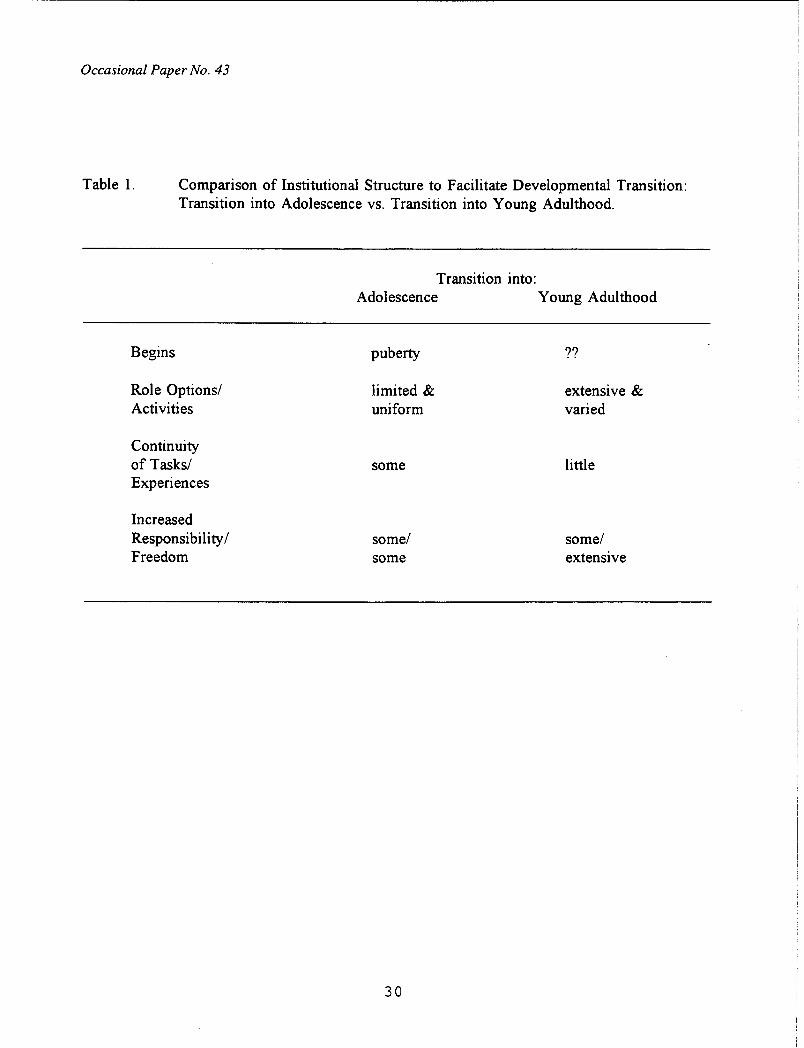
Occasional Paper No. 43
Table 1. Comparison of Institutional Structure to Facilitate Developmental Transition: Transition into Adolescence vs. Transition into Young Adulthood.
Transition into: Adolescence Young Adulthood
Begins puberty ??
Role Options/ Activities
limited & uniform
extensive & varied
Continuity of Tasks/ Experiences
some little
Increased Responsibility/ Freedom
some/ some
some/ extensive
30

]uapn]s auul IIy f! Jay)!au aq 01 juapuodsal JOJ L.msaDau SBM I! ‘dnol% paii!umom,un aqi u! papnpu! aq 0~ ‘q e(s)lualed s,asnods yqm %u!A!I aq IOU pIno:, luapuodsal ‘(s)wa.wd UMO ~I!M %I!A!I IOU 0) uo!~ppe UI ‘B
‘z(j-gL61 = sJ.loqo:, !pEI‘jz = u paly%!aM -0~ lo saL Jaqqa = -- fou = N !saL = A
‘ZZ-12 a&? = E aAl?M !OZ-(3 ai% = 2 aAEM :aJON
N?PN
N’8N
N?‘i’N
N??N
N9N
N’8N
N%‘N
N9N
m
itfEs!E
NT?N
NPN
N%‘N
NS’N
N??N
N??N
-- D --
-- 27 -- -- 78 --
-- D --
-- ‘8 --
g$fgg&
$$&ggj
ftiiBB#
N?S’N
N%‘N
N%‘N
-- D --
-- T --
-- 18 --
-- T --
-- 79 --
-- D --
I’S2
I ‘PI
S’P
L’L
0'6
9-c
L'L
9'E
S'S
I'S
% c91
wo -_-------------_--_-__________ pallymuo~q
luamd aI%!s
p1!q3 ou ‘pa!.mfi
h?Me/awoy-paAoIdwzJ
auroy-padoIdurg
deMe/awoy-a%aIIoa
away-a8aI103
'II
'01
'6
'8
'L
'9 l-l m
'S
'9
't
'Z
'I
(E/Z =w stiyqs
ppqq
(E/Z aA’=‘) (s)luaJed
ql!M aA!T
k/Z aAeM) paAoIdwa aw wd
k/Z aAeM) luapnls
am!1 IIW
aIdcues JO a8slua3lad
dnol3
*sa%epaxad pm suoggap dnolg :pooylInpe %unoA olu! sywd ajg *z aIqel

Table 3. Summary of Measures
Scale/Item Description/Sample Item Total Sample Means (standard deviations) Wave 1 Wave 2 Wave 3
Well Being
Life Satisfaction Self Esteem Self Derogation Self-efficacy Fatalism Social Support Loneliness
Substance Use W N
Cigarette Use Alcohol Use
Binge Drinking
Marijuana Use
How satisfied are you with your life as a whole these days?” I take a positive attitude toward myself.b I feel my life is not very useful.b When I make plans, I am almost certain I can make them work.b Every time I try to get ahead, something or somebody stops me.b There is always someone I can turn to if I need help.b I often wish I had more good friends.b
4.95 (1.21) 4.95 (1.21) 4.20 (3) 4.26 (.57) 2.03 (.75) 1.84 (.73) 3.86 (.68) 3.92 (.69) 2.08 (.73) 1.97 (.72) 4.28 (.70) 4.41 (-63) 2.94 (.88) 2.77 (.90)
How frequently have you smoked cigarettes during the past 30 days?c 1.66 (1.24) On how many occasions have you had alcoholic beverages to drink
during the past 30 days?d 2.49 (1.51) Think back over the last two weeks. How many times have you had
five or more drinks in a row?e 1.75 (1.22) On how many occasions (if any) have you used marijuana or hashish
during the past 12 months?d 2.15 (1.93)
1.78 (1.40)
2.76 (1.57)
1.84 (1.26)
2.23 (1.99)
4.97 (1.22) 4.31 (.56) 1.72 (.70) 4.01 (.66) 1.91 (.71) 4.41 (.62) 2.66 (.87)
1.84 (1.49)
2.92 (1.58)
1.87 (1.26)
2.17 (1.97)
Note. Total sample includes senior year cohorts 1976-92 (N = 21,134 for substance use measures; N = 3,586 for the well-being measures); modal ages were 18, 19-20, and 21-22, for the three waves, respectively.
a. possible responses ranged from 1 (completely dissatisfied) to 7 (completely satisfied) b. possible responses ranged from 1 (disagree) to 5 (agree) c. possible responses ranged from 1 (not at all) to 7 (two packs or more per day) d. possible responses ranged from 1 (0 occasions) to 7 (40 or more) e. possible responses ranged from 1 (none) to 6 (ten or more times)

Life-Paths into Young Adulthood
Table 4. Overview of Repeated Measures ANOVAs Results for Well-Being and Substance Use.
Well-Being Substance Use ---------------------------------------------------------------------------- -_---_____---______-_________________^_
Life Sat.
Self- Self- Self- Social 30day 30day Binge 12mo. Esteem Dero. Effc. Fatal. Sup. Lone. Cig. Ale. Drink. Marij.
Between-Subiects Effects
Cohort (C) Gender (G) *** *** ** *** ** Life Path (P) *** *** *** *** *** *** C*G * c*p G*P * C*G*P
Within-Subiects Effects
Age (4 linear quadratic
C*A linear quadratic
G*A linear quadratic
P*A *** linear ** quadratic *
C*G*A linear quadratic
C*P*A linear quadratic
G*P*A linear quadratic
C*G*P*A linear quadratic
*** *** *** *** *** *** *** *** *** *** *** ***
**
* * ** *
* * ** **
**
**
** **
* **
*** *** *** *** * *** *** *** *** *** *** ***
* *** ** ** *** *** ** *** * *
*** *** *** *** *** *** *** * *** * ***
** *** ** *** *** * ***
*** ** ***
*** *** *** *** *** *** *** ***
*** *** *** *** *** *** *** *** ** *** *** ***
*** * *** *
Note. See Tables A-l and A-2 in Appendix for a full summary of the analyses and fmdings. *** = p<.OOl, ** = pc.01, * = pc.05.
33

Occasional Paper No. 43
Table 5. Summary of Significant Overall Cohort and Cohort by Age Effects
a. Overall Cohort Effects (averaged across age)
Cigarette Use 1>2=3 Alcohol Use 1>2>3 Binge Drinking 1 > 2 > 3 Marijuana Use 1 > 2 > 3
b. Cohort by Age Interactions: Age-Change Coefficients
Age and Cohort Effects
Age-Change Coefficients ----------------------------------------------------------------------------------------------------------------------------
Self- 30 day 30 day Binge 12 month Efficacy Fatalism Cigarette Alcohol Drinking Marijuana
Linear Age Effects:
Overalla .11*** -. 13*** .14*** .27*** .06*** -.02* Interactionsb
lv2 .05* -.04 .04* -- .oo .11*** lv3 .08** -. 13*** .07*** -- -.05* .03 2~3 .03 -.08* .03 -- -.05* -.08**
Ouadratic Age Effects:
Overalla Interactionsb
lv2 lv3 2~3
.02 .oo -.03*** -.02* .oo -.05***
-- __ -- -.Ol -.03 -.06** -- -- -- -.05* -.06** -.08*** -- __ _- -. 10*** -.03 .02
Note. Cohort 1 = 1976-81; Cohort 2 = 1982-86; Cohort 3 = 1987-92 a. These age-change coefficients are for the total sample. Significant positive and negative linear effects refer to
linear-shaped age-related increase and decrease, respectively; significant positive and negative quadratic effects refer to U-shaped and inverted U-shaped age-related patterns, respectively.
b. These age-change coefficients represent paitwise comparisons of age-related change in each cohort. Significant positive and negative linear coefficients refer to significantly more positive and negative age-related linear change, respectively, in the fast cohort in the comparison versus the second; significant positive and negative quadratic coefficients refer to significantly more positive and negative quadratic effects, respectively, in the first cohort in the comparison versus the second. The third comparison was obtained in post-hoc analyses.
34

Life-Paths into Young Adulthood
Table 6. Summary of Significant Overall Gender and Gender by Age Effects
a. Overall Gender Effects (averaged across age)
Self Esteem m>f Self Derogation m<f Self Efficacy m>f Social Support m<f Loneliness m<f
Cigarette Use m<f Alcohol Use m>f Binge Drinking m>f Marijuana Use m>f
b. Gender by Age Interactions: Age-Change Coefficients
Age and Gender Effects
Age-Change Coefficients --------__----------____________________------------------------------------------------------------------------------------
Self- Social 30 day 30 day Binge 12 month Efficacy Support Cigarette Alcohol Drinking Marijuana
Linear Age Effects:
Overalla Interactionb
mvf
.11*** .11*** .14*** .27*** .06*** -.02*
_- .08** .08*** .17*** .09*** .08***
Ouadratic Age Effects:
Overalla Interactionb
mvf
.02 .oo -.03*** -.02* .oo -.05***
-.08** _- -- __ -- --
a. These age-change coefficients are for the total sample. Significant positive and negative linear effects refer to linear-shaped age-related increase and decrease, respectively; significant positive and negative quadratic effects refer to U-shaped and inverted U-shaped age-related patterns, respectively.
b. These age- change coefficients represent gender comparisons of age-related change. Significant positive and negative linear coefficients refer to significantly more positive and negative linear age-related change, respectively, for males than for females; significant positive and negative quadratic coefficients refer to significantly more positive and negative quadratic effects, respectively, for males than for females.
35
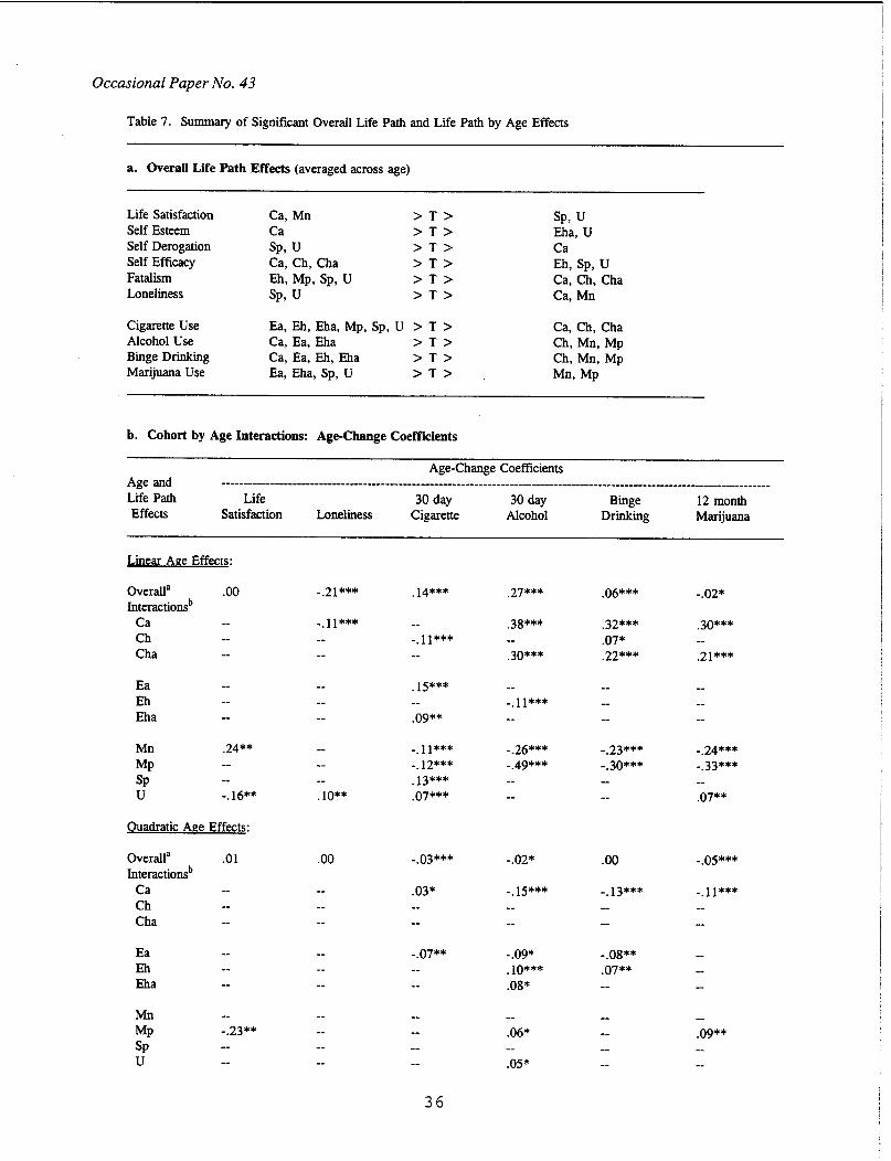
Occasional Paper No. 43
Table 7. Summary of Significant Overall Life Path and Life Path by Age Effects
a. Overall Life Path Effects (averaged across age)
Life Satisfaction Ca, Mn >T> SP, U Self Esteem Ca >T> Eha, U Self Derogation SP, U >T> Ca Self Efficacy Ca, Ch, Cha >T> Eh, SP, U Fatalism Eh, MP, Sp, U >T> Ca, Ch, Cha Loneliness SP, U >T> Ca, Mn
Cigarette Use Ea, Eh, Eha, Mp, Sp, U > T > Ca, Ch, Cha Alcohol Use Ca, Ea, Eha >T> Ch, Mn, Mp Binge Drinking Ca, Ea, Eh, Eha >T> Ch, Mn, Mp Marijuana Use Ea, Eha, Sp, U >T> Mn, MP
b. Cohort by Age Interactions: Age-Change Coefficients
Age-Change Coefficients Age and --______________________________________-------------------------------------------------------------------------------~---- Life Path Life 30 day 30 day Binge 12 month Effects Satisfaction Loneliness Cigarette Alcohol Drinking Marijuana
Linear Age Effects:
Overalla Interactionsb
Ca Ch Cha
.oo
-- -- --
Ea -- Eh -- Eha --
Mn .24** MP -- SP -- U -. 16**
Quadratic Age Effects:
Overalla Interactionsb
Ca Ch Cha
.Ol
-- -- --
Ea -- Eh -- Eha --
Mn -- MP -.23** SP -- U --
-.21***
-.11*** -- --
-- -- --
-- -- -- .10**
.oo
-- -- --
-- -- --
-- -- -- --
.14*** .27*** .06*** -.02*
.30*** -- .21***
.38*** .32*** -- .07* .30*** .22***
-- -.11*** --
.15*** -- .09**
-- -.11*** _-
-- -- --
-- --
-.11*** -. 12*** .13*** .07***
-.26*** -.49*** --
-.23*** -.24**” -.30*** -.33*** -- -- -- .07**
-.03***
.03* -- --
-.07** --
-.02* .oo
-.13*** --
-.05***
-.11*** __ --
-.09* . IO*** .08*
-.08** .07**
-- -- -- --
-- .06* -_ .05*
-- .09** -- -_
--
36
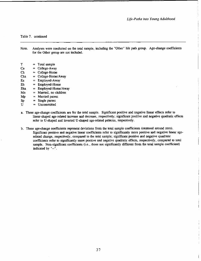
Life-Paths into Young Adulthood
Table 7. continued
Note. Analyses were conducted on the total sample, including the “Other” life path group. Age-change coefficients for the Other group are not included.
T = Total sample Ca = College-Away Ch = College-Home Cha = College-Home/Away Ea = Employed-Away Eh = Employed-Home Eha = Employed-Home/Away Mn = Married, no children MP = Married parent SP = Single parent U = Uncommitted
a. These age-change coefficients are for the total sample. Significant positive and negative linear effects refer to linear-shaped age-related increase and decrease, respectively; significant positive and negative quadratic effects refer to U-shaped and inverted U-shaped age-related patterns, respectively.
b. These age-change coefficients represent deviations from the total sample coefficients (centered around zero). Significant positive and negative linear coefficients refer to significantly more positive and negative linear age- related change, respectively, compared to the total sample; significant positive and negative quadratic coefficients refer to significantly more positive and negative quadratic effects, respectively, compared to total sample. Non-significant coefficients (i.e., those not significantly different from the total sample coefficient) indicated by “--‘I.
37

Life-Paths into Young Adulthood
FIGURES
39
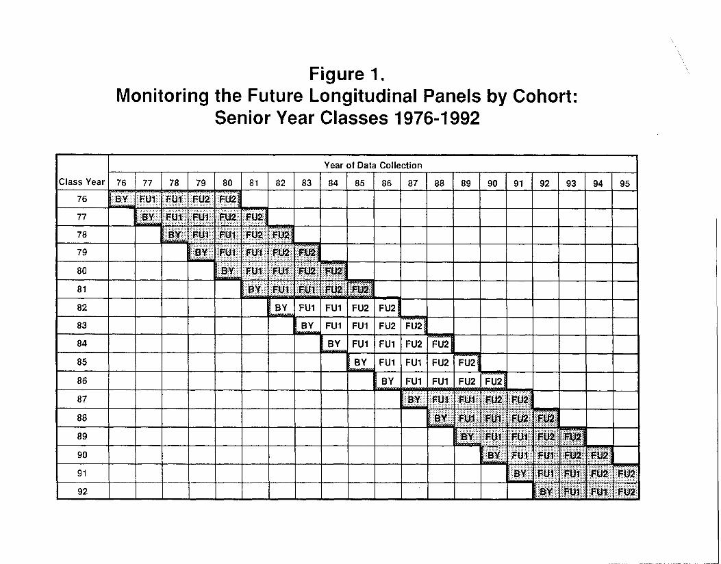
Figure 1. Monitoring the Future Longitudinal Panels by Cohort:
Senior Year Classes 19764992
I I I
Year of Data Collection
Class Year 76 77 78 79 80 ai a2 a3 a4 a5 a6 a7 88 a9 90 91 92 93 94 95
a2
a3
a4
a5
86
a7
aa
a9
91
92 It

5
4.9
4.8
4.7
4.6
4.5
4.4
4.3
4.2
4.1
4
3.9
3.8
3.7
3.6
3.5
Figure 2. Change in Well-Being during the Transition to Young Adulthood:
Total Sample
I.
A
l w l
.-_-___-__-_----__-________________
.__-___-___------_-________________
.______--___-----_--_______________
.---__------- - - - -_--_------_- ----__
.______-___------_--_______________
.-__-__-----_-------------
A-----------
.--_--_--___-_-_
*Satisfaction with Life i-Self-Esteem
+-Self-Efficacy 0 Social Support
_-_______-_-______
_-___-__-_________
Wave 1 Wave 2 Wave 3 (19-20) (21-22)
3
2.9
2.8
2.7
2.6
2.5
2.4
2.3
2.2
2.1
2
1.9
1.8
1.7
1.6
1.5
8 Fatalism 1- -----_-__-______-____ I f Loneliness I I
I I I
Wave 1 Wave 2 Wave 3 (W (i 9-20) (21-22)

Figure 3. Change in Substance Use
during the Transition to Young Adulthood: Total Sample
3
2.9
2.8
2.7
2.6
2.5
2.4
2.3
2.2
2.1
2
1.9
1.8
1.7
1.6
1.5
+30-Day Cigarette Use 830-Day Alcohol Use X2-Week Binge Drinking
f 12-Month Marijuana Use
----_---___________
/
------------ ----______
/
----- ______--------___
_______________________ _______-______-----_____________________--- d ---------- -------------_____--____________ ______---__------_______________________---
___________---__________________________---
___________-______________________
_________ /-
____---__----- __-_______-________
Wave 1
(18)
Wave 2 Wave 3 (19-20) (21-22)

Figure 4. Cohort Differences in Well-Being during the Transition to Young Adulthood:
Self-Efficacy and Fatalism
4.2 2.4
3.6
3.5
__________________________
_____-__-----_-____-_____________
Wave 1
(18) Wave 2 Wave 3 (19-20) (21-22)
2.3
2.2
5 2.1 .- 3 ?ii IL
2
1.9
1.8
1.7
__________________________
--__e___
I I I
Wave 1 Wave 2 Wave 3 (18) (19-20) (21-22)
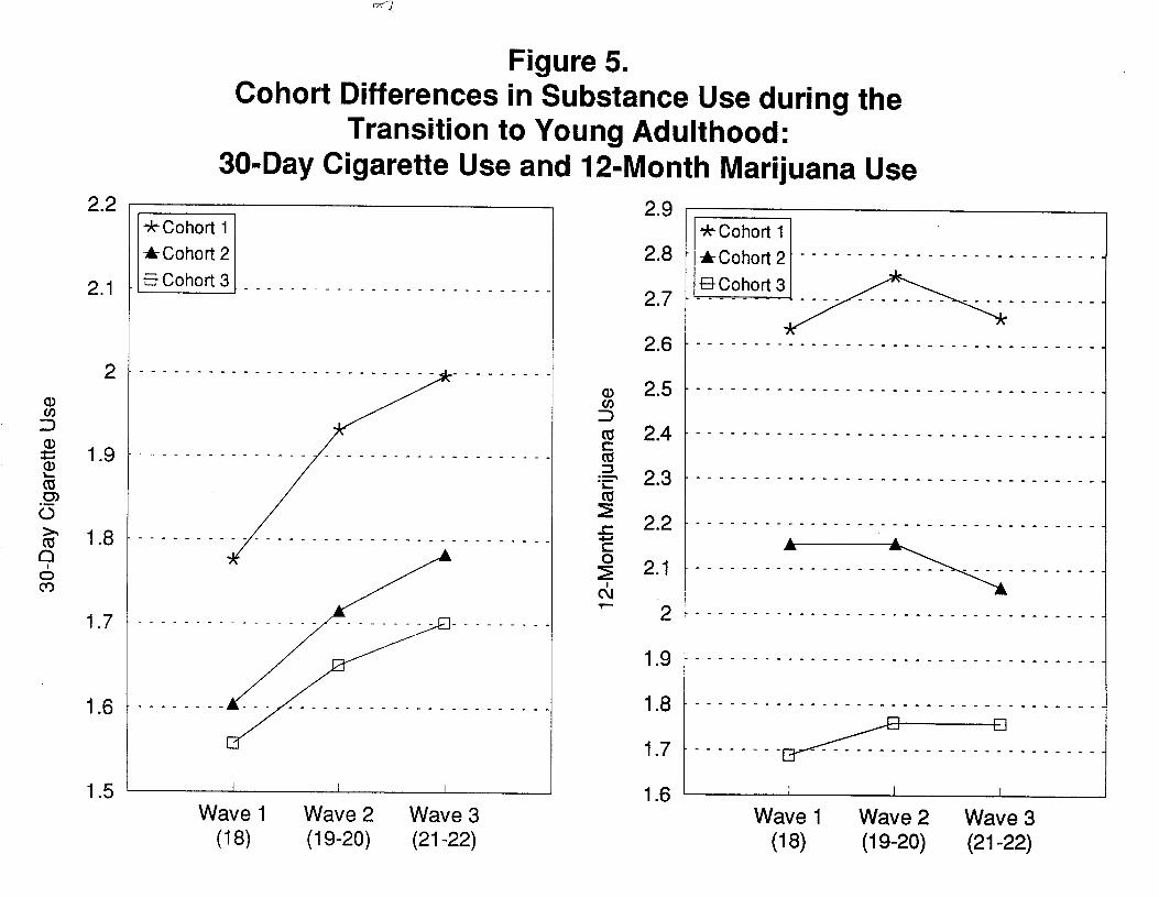
2.2
2.1
2
1.9
1.8
1.7
1.6
1.5
Figure 5. Cohort differences in Substance Use during the
Transition to Young Adulthood: 30-Day Cigarette Use and 12-Month Marijuana Use
*Cohort 2 1
5Cd-m-t 3j _ _ _ _ _ _ _ _ _ _ _ _ _ _ _ _ _ _ _ _
I I I
Wave 1 Wave 2 Wave 3 (18) (19-20) (21-22)
2.9
2.8
2.7
2.6
2.5
2.4
2.3
2.2
2.1
.2
1.9
1.8
1.7
1.6
,--------------_--______ -_---------
-------_---_--__-___---- -__----_-_
----------------_---_____ - - - - - - - - -
__-----_---_-__^_______ -----------
__-----_---_--__-_______
__-_---------_---_--_____ -_-----_-
____--__--_--__--_-_______ -_------
____-___--_-____-__-__________ - - - - 3
____________ - - - - -
I I I
Wave 1 Wave 2 Wave 3 tw (19-20) (21-22)

3.2 2.2
3.1
3
2.9
z 3 2.8 5 s g a 27 - ii? Q d 2.6 c9
2.5
- - - - - _ -
- - - - - - -
- - - - - _ _
- - - - - - -
- - - _ _ _ _
- - - - - _ -
- - - - - _ _
2.4 __-_--_-_______ ______
/
__-_---__-___
2.3
2.2
-_--------- ----_--_--__
/
_______--__
1.6 .___________________________________
Wave 1 Wave 2 Wave 3 (18) (19-20) (21-22)
1.5 I
Figure 6. Cohort Differences in Substance Use during the
Transition to Young Adulthood: 30-Day Alcohol Use and 2-Week Binge Drinking
----___
---____
I I I
Wave 1 Wave 2 Wave 3 (18) (19-20) (21-22)

. . I
I t
t
I
I I
I
I I t
uoddns ppos
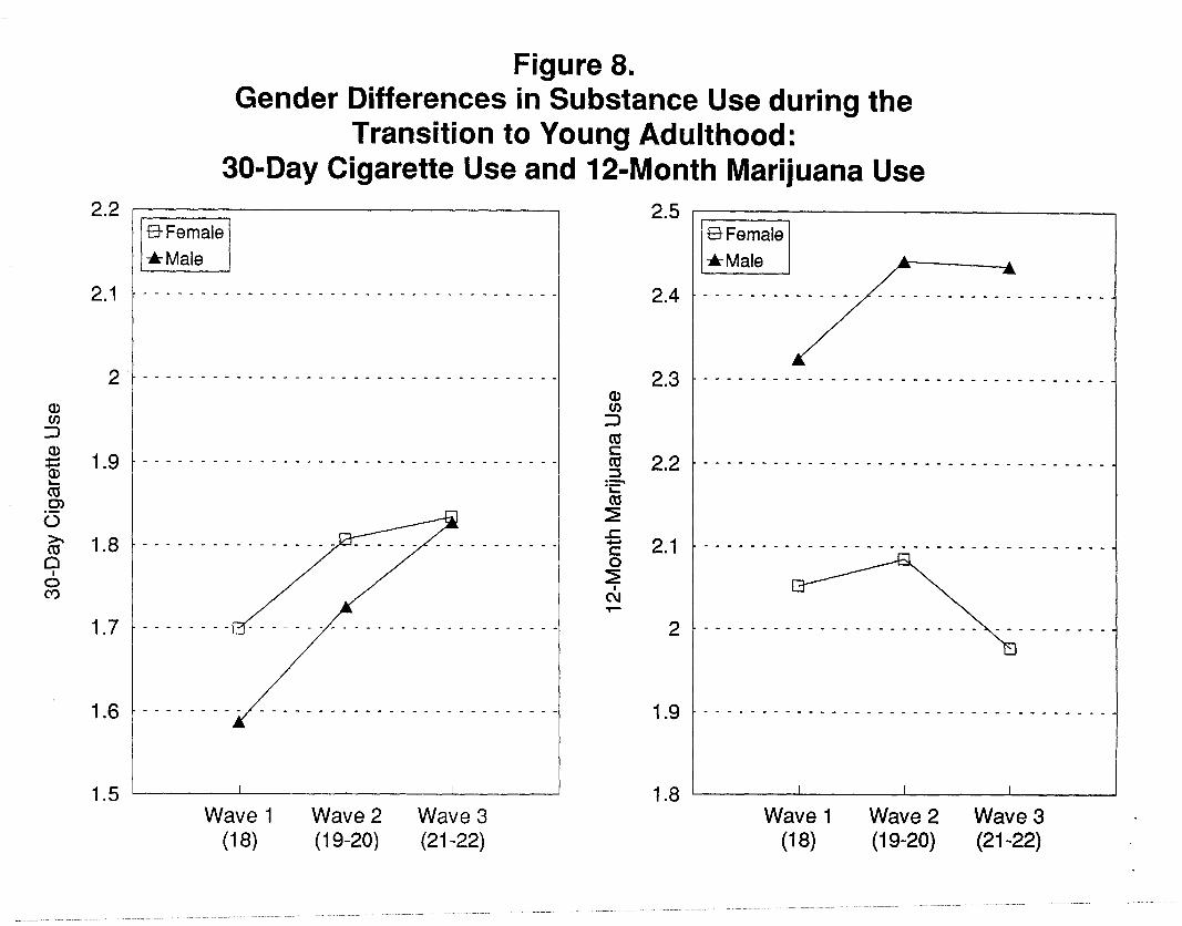
1.8
1.6
Figure 8. Gender Differences in Substance Use during the
Transition to Young Adulthood: 30-Day Cigarette Use and 12-Month Marijuana Use
Wave 1 (18)
Wave 2 Wave 3 (19-20) (21-22)
2.4 . - - - - %yx -------_ 2.3 ___________________________________ I 2.2 t-----------------------------------
---v-e_
:‘:::-:I”\;-; - - -s- -e
1.8 ’ I I I
Wave 1 Wave 2 Wave 3 (18) (19-20) (21-22)
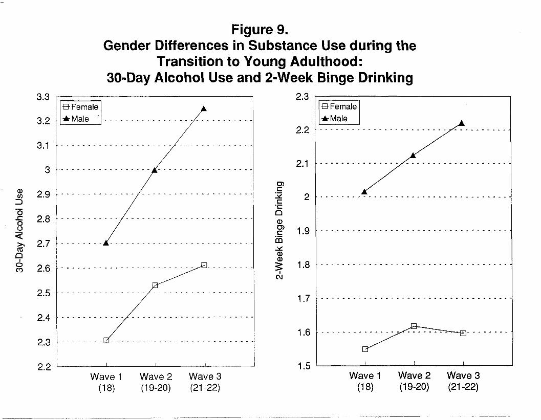
3.3
3.2
3.1
3
2.7
2.6
2.4
2.3
Figure 9. Gender Differences in Substance Use during the
Transition to Young Adulthood: 30,Day Alcohol Use and 2-Week Binge Drinking
- - - -__ - - - - - - - - -_ - - -__--ame-----_--
9
Wave 1 (18)
Wave 2 Wave 3 (19-20) (21-22)
2.3 r
2.2
2.1
1.8
1.6
f3 Female (
Wave 1 Wave 2 Wave 3 (18) (19-20) (21-22)

.
Figure IO. Life Path Differences in Well-Being
during the Transition to Young Adulthood: Satisfaction with Life
5.5
5.4
5.3
5.2
5.1
5
4.9
4.8
4.7
4.6
---_--L------__-_-_________ _---_-___--_-___
/ /
_______________-_-______________________----
--ic------ ̂--__-__---_-_-___--_______
\
_-_----____-______________ ______-_-__--_____
Wave 1 (18)
Wave 2 Wave 3 (19-20) (21-22)

Figure 11. Life Path Differences in Well-Being
during the Transition to Young Adulthood: Loneliness
3.2
3.1
3
2.9
cn
?i 2.8
.- i! 4 2.7
2.6
2.5
2.3
I 0 College, Away ____________________---------- -EtUncommitted
----------
Wave 1 (18)
Wave 2 Wave 3 (19-20) (21-22)

Figure 12. Life Path Differences in Substance Use during the Transition to Young Adulthood:
30-Day Cigarette Use
2.4
2.3
2.2
2.1
% 3 2
1.6
1.5
1.4
1.3
Post-High School Education Employment Marriage and Children
-_------_---_---_---______
I I I
Wave 1 Wave 2 Wave 3 (18) (19-20) (21-22)
.I
-_--------_--__- -- _---- p” -_---------- ------------ -__--__--_ --__--_---_--__ - - - - _
- - - - -
- - - - -
-- _________ _ d ---- -- ----_-- 6 --- ------ --^- --- ___-_--____ - - - - -
-_----__--_---_---- ------_
1 ff Uncommitted I I I
Wave 1 Wave 2 Wave 3 Wave 1 Wave 2 Wave 3 (18) (19-20) (21-22) (18) (19-20) (21-22)

Figure 13. Life Path Differences in Substance Use during the Transition to Young Adulthood:
30-Day Alcohol Use
Post-High School Education
3.4 / jlTotalSample p 3.3 .
3.2 .
3.1 -
3 -
2.8 - - _ _ _ _
2.7 _ _ _ _ _ _
2.6 . _ _ _ _ _
2.5 . - - - - -
2.4 . _ _ _ _ _
2.3 . _ _ _ _ _
-__-------_--- -
_____---__ -_-_
------- -_---___
-__- ----__-__ _
*
- -- ------_ _--
-- -----_ ---_-_
- ---------_____
,‘I: j ------ Jsm; ------,------
Wave 1 Wave 2 Wave 3 (18) (19-20) (21-22)
Employment -_------_-___-___- ------ 74 -_--_--__-__ --- -___--___
-Total Sample - - - - - - _ _ _
@Working, Away - - - - - - - - - eworking, Home
#Working, Home then Away - - - - - - - - - @Uncommitted
I I I Wave 1 Wave 2 Wave 3
(18) (19-20) (21-22)
Marriage and Children
~::::::::-::
Wave 1 (18)
Wave 2 (19-20)
Wave 3 (21-22)

Figure 14. Life Path Differences in Substance Use during the Transition to Young Adulthood: -
2-Week Binge Drinking
2.3
2.2
2.1
2
1.9
1.8
1.7
1.6
1.5
1.4
Post-High School Education Employment Marriage and Children
I-
-Total Sample EXollege, Away +College, Home VCollege,
Home then Away
---------- -____--________
/,
Wave 1 Wave 2 Wave 3 (18) (19-20) (21-22)
-_------_------__---_______ e -_---- -- --_-_ __-________ __-_--__------__-_-------- 4
_______----__-__-__-______ 4
rTotal Sample __________
$I Working, Away &Working, Home XWorking, Home then Away - - - - - - - - - EIUncommitted
I 1 I Wave 1 Wave 2 Wave 3 Wave 1 Wave 2 Wave 3
(18) (19-20) (21-22) (18) (19-20) (21-22)
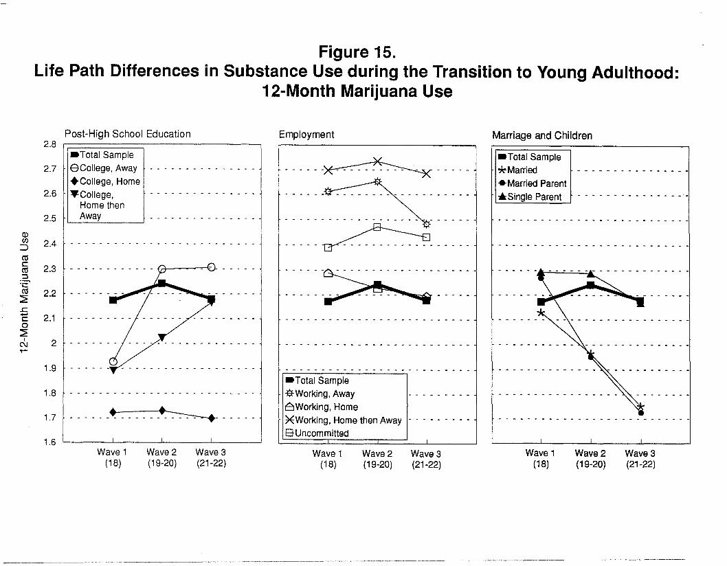
Figure 15. Life Path Differences in Substance Use during the Transition to Young Adulthood:
12-Month Marijuana Use
2.8
2.7
2.6
2.5
If: 3 24 *
g 2 2.3 := 2
z 22 . AZ E 2.1
8 & 2 T-
1.9
1.8
1.7
1.6
Post-High School Education Employment Marriage and Children
rTotal Sample CKollege, Away Wollege, Home VCollege,
Home then Away
________-____- - -___-______
I I I
Wave 1 Wave 2 Wave 3 (18) (19-20) (21-22)
-____---_----------------- 1 -____---_-----------------
i --______-________
-Total Sample
Wave 1 Wave 2 (18) (19-20)
Wave 3 (21-22)
_ _ _ _ _ _ _ _ _ _ _ _ _ _ _
*Married Parent *Single Parent - - - - - - - - - - - - - _ _’
Wave 1 (18)
Wave 2 (19-20)
Wave 3 (21-22)

Life-Paths into Young Adulthood
55
APPENDIX
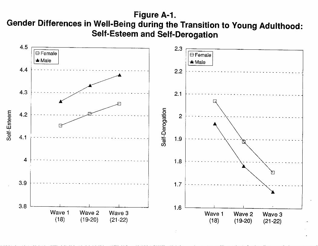
P 0

I I I

.
Figure A-3. Life Path Differences in Well-Being
during the Transition to Young Adulthood: Satisfaction with Life
5.5
5.4
5.3
5.2
5.1
5
4.9
4.8
4.6
+ Total Sample 8 College, Away 3t Married + Married Parent *Single Parent Q- Uncommitted
__________
____--_---
I I I
Wave 1 Wave 2 Wave 3

Figure A-4. Life Path Differences in Well-Being during the Transition to Young Adulthood:
Self-Esteem and Self-Derogation 4.5
4.4
E 4.3
tii 7-l LLI
4.1
+Total Sample QCollege, Away X Working, ! Home then Away Ef “ncommitted - - - - - - - - - - - - - - - _ - - - - -
---w___
Wave 1 Wave 2 Wave 3
PI (19-20) (21-22)
2.3
2.2
2.1
2
1.9
1.8
1.6
1.5 Wave 1 Wave 2 Wave 3
w (19-20) (21-22)

Figure A-5. Life Path Differences in Well-Being during the Transition to Young Adulthood:
Self-Efficacy and Fatalism -Total Sample %ollege, Away +College, Home f College,
Home then Away eworking, Home &Single Parent q Uncommitted
-Total Sample @2ollege, Away
I
+College, Home VCollege,
Home then Away
4.2
4.1
3.8
3.6 I I I
Wave 1 Wave 2 Wave 3 (18) (19-20) (21-22)
2.4
2.3
2.2
2.1
E co .- 5 2 iii LL
1.9
1.8
1.6
.------- ---- ---__ < ._----- ---------_ - - .__-----__ ___-_____ ?l Wave 1 Wave 2 Wave 3
(18) (19-20) (21-22)
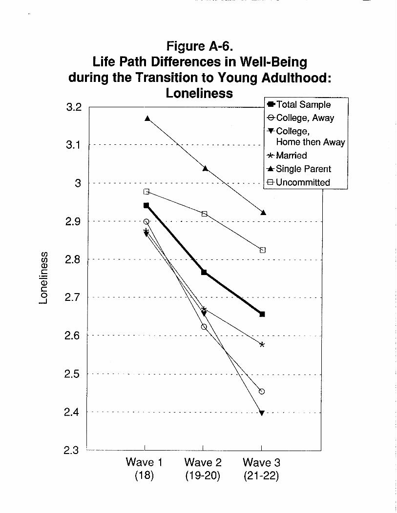
Figure A-6. Life Path Differences in Well-Being
during the Transition to Young Adulthood:
3.2
3
2.9
2.6
2.5
2.4
2.3
Loneliness +Total Sample
ecollege, Away
+-College, Home then Away
*Married
*Single Parent
EI- Uncommitted I
Wave 1 (18)
I I
Wave 2 Wave 3 (19-20) (21-22)


![21st Century[1].Jerald](https://img.pdfslide.net/doc/110x75/552101504a795963718b4a0f/21st-century1jerald.jpg)

