A TIRE CONTACT SOLUTION TECHNIQUE

John T. Tielking Civil Engineering Department

Texas A&M University

EXPANDED ABSTRACT

An efficient method for calculating the contact boundary and interfacial pres- sure distribution has been developed. This solution technique utilizes the discrete Fourier transform to establish an influence coefficient matrix for the portion of the pressurized tire surface that may be in the contact region. This matrix is used in a linear algebra algorithm to determine the contact boundary and the array of forces within the boundary that are necessary to hold the tire in equilibrium against a specified contact surface. The algorithm also determines the normal and tangential displacements of those points on the tire surface that are included in the influence coefficient matrix. Displacements within and outside the contact region are calculated.

The solution technique is implemented here with a finite-element tire model that is based on orthotropic, nonlinear shell of revolution elements which can respond to nonaxisymmetric loads (refs.1, 2). The basic characteristics of this relatively comprehensive tire model are described in reference 3. This presentation will focus on the contact solution technique published in reference 4. A sample contact solution is presented for the 32 X 8.8 Type VII aircraft tire that was studied in reference 5.

95

https://ntrs.nasa.gov/search.jsp?R=19830013124 2019-03-02T10:04:29+00:00Z

FINITE-ELEMENT TIRE MODEL

The tire is modeled by an assemblage.of axisymmetric curved shell elements. The elements are connected to form a meridian of arbitrary curvature and are located at the carcass midsurface. Figure 1 shows the assembly of 21 elements along the midsurface of a G78-14 tire, for which calculated results are shown in this paper. A cylindrical coordinate system is used, with r, 0, and z indicating the radial, circumferential, and axial directions, respectively. Each element forms a complete ring which is initially axisymmetric with respect to z. The elements are connected at nodal circles, hereafter referred to as nodes.

The finite elements are homogeneous orthotropic with a set of moduli specified for each individual element. The orthotropic moduli for each element are determined by the ply structure surrounding the element. Each ply (on each element) is speci- fied separately, thereby allowing the model to include carcass details such as an overhead belt, sidewall reinforcement, and turnups. A turnup is included in the G78-14 tire model. It was found necessary to include the turnup in the model to obtain the correct inflated shape.

96

. . .

14

12

11

R ( 1 in

10

E

ad at 32 psi

Inner Surface

Finite Elements

Rim

1 z 3 -r

Z (in)

Figure 1

97

SINGLE HARMONIC RING LOADS

The finite element tire model will respond to single harmonic ring loads on the nodal circles. An approximately linear load-deflection response is obtained when an individual ring load is applied to any node of the pressurized tire model. An example ring load-deflection calculation for the 678-14 tire model is shown in figure 2. A harmonic sequence of stiffness matrices is obtained by applying a sequence of single harmonic ring loads to each of the nodes that may be in the tire-pavement contact region.

0 0.5 I .o 1.5

RADIAL DEFLECTION (in)

CROWN LOAD-DEFLECTION DATA CALCULATED WITH A UNIFORM RING LOAD APPLIED TO THE CROWN NODE

SINGLE HARMONIC RING LOADS APPLIED TO A FINITE ELEMENT NODE

Figure 2

98

TRANSFER-FUNCTION DEFINITION

As a consequence of the linearity of the ring load-deflection response, the application of a single harmonic ring load produces a displacement field that varies circumferentially in the same harmonic as the applied ring load. Figure 3 gives the definition of the transfer function T, as the ratio of the output and input amplitudes. Since each node responds differently, a transfer-function matrix, Tik]n' is needed to store the stiffness information generated by the ring loads.

INPUT: Single Harmonic Ring Load A, cos no

OUTPUT: Single Harmonic Displacement B, cos n0

Bn TRANSFER FUNCTION T, = A n

Tikjn = nth harmonic transfer function relating displacement of node i to an nth harmonic ring load on node k

Figure 3

99

POINT LOAD VECTOR {p) AND THE DISCRETE FOURIER TRANSFORM (DFT)

This application of the discrete Fourier transform uses an even number of points (N), equally spaced around the circumference. The example shown in figure 4 uses N = 8 points. A unit load is applied at any point, say point 0. The DFT of the load vector yields a set of N coefficients, G-, J which are approximate values of the coefficients of the conventional Fourier series defined on the continuous interval 0 I 8 I HIT and representing the unit point load. The point load is applied, sequentially, in the radial, axial, and circumferential directions.

INFLUENCE COEFFICIENT GENERAT ION

(pi = 11, 0, 0, 0, 0, 0. 0, 0) load vector

DFT Gj = 1'3 gk$k N k=c) 'e = e-i2n'N

gk = 1Pt , Gj = b j = 0, 1, . . ., N-l

Figure 4

100

INVERSE DISCRETE FOURIER TRANSFORM (IDFT) AND THE INFLUENCE COEFFICIENTS

Having the unit point load represented by a conventional Fourier series, whose coefficients a, are approximately given by the DFT coefficients, the transfer func- tions Tikln are used, on each harmonic, to obtain the coefficients b, of the Fourier series representing the response of the nodal circle to the unit point load. The inverse discrete Fourier transform is then used to evaluate the displacements, um, at the N points. These displacements are the elements of the influence coefficient matrix [Aijkal as Seen in figure 5.

1 INPUT SERIES COEFFICIENTS an 2 Gn = H

IT OUTPUT SERIES COEFFICIENTS bn = anTik,n = N ik,n

DFT OF DISPLACEMENT VECTOR Gn = bn

ik = N-l

IDFT um c GnWemn m = 0, 1, . . ., N-l n=O

INFLUENCE COEFFICIENTS ik Aijk, = uj-, j = 1, 2, . . ., N

SHIFT: ik .

Aijke = 'j-l J = t,L+l, . . ., N

SYMMETRY: Akeij = Aijke

Figure 5

101

INFLUENCE COEFFICIENT MATRIX

The influence coefficient matrix relates the radial, axial, and circumferential components of the displacement of points on the tire surface to the radial, axial, and circumferential components of load at these points. The radial response parti- tion shown in figure 6 is used to obtain a solution for frictionless contact, in which the axial and circumferential force components are known to be zero. The matrix here covers 3 points on each of 5 nodes. The point separation with this matrix is 11.25 degrees.

'k,, q load at point II on node k

d ij = deflection of point j on node i

dll

d21

d31

d41

d!il

d12

d22

d32

d42

d52 . -

- -

All11

A2111

A3111

f+4 111

A5111

A1211

A2211

A3211

A4 211

A5211 -

A2121

A3121

A4 121

b 121

A1221

A2221

A3221

4 221

A5221

A3131

h 131

a5131

A1231

A2231

A3231

A4 231

A5231

b 141

A5141

A1241

A2241

A3241

Ib 241

A5241

{dij> = [hjke]

A5151

A1251 A1212

A2251 A2212

A3251 A3212

h251 b212

AFj 251 A5252

A2222

A3222

J% 222

A5222

A3232

h 232 h242

&J 232 4242 %

r-

pll

p21

p31

p41

p51

p12

p22

'32

p42

'52 mm

.

Figure 6

102

TOROIDAL SHELL CONTACT SCHEMATIC

After the inflation solution has been obtained, the tire model is deflected against a frictionless, flat surface. The contact surface is perpendicular to the wheel plane of symmetry and located at the specified loaded radius RL, as shown in figure 7. The vertical load and the contact boundary are unknown a 'priori.

Figure 7

103

RADIAL DEFLECTIONS IN THE CONTACT REGION

When the radius RR is specified, the radial deflections are given approximately . .

2 f'h,N = Ri cos [(j -l)Ae] - Ra, where Ri is the inflation radius of node i and

is the point spacing. Since the contact half-angle is usually less than 2o”, the error in approximating the radial deflections by the above equation is not large. An initial estimate of the contact boundary is taken as the geometric intersection of the tire model and the contact surface. (See fig. 8.)

, NODE I

--m

CONTACT SURFACE

Figure 8

104

LINE LOAD VECTORS

The radial deflections within the contact boundary are known but the forces that produce these deflections are unknown. The tangential (axial and circumferen- tial) deflections within the contact boundary are unknown but the tangential forces are zero because the contact is frictionless. All surface forces are zero outside of the contact boundary. Since the number of unknowns (deflections and loads) is less than or equal to the number of equations established by the influence coeffi- cient matrix, an initial contact solution can be found. The contact boundary is then adjusted to exclude negative radial forces. Three to five boundary adjustments are normally needed to converge on the contact solution. Figure 9 shows the load vectors obtained in a solution for the G78-14 tire with 221 kPa (32 psi) inflation pressure. The elements of {p) are values of the line load at 32 points on the tire model equator. The other vectors give line load values in the right (and left) half of the contact region. Seven nodal circles are in the contact region in this ex- ample.

105

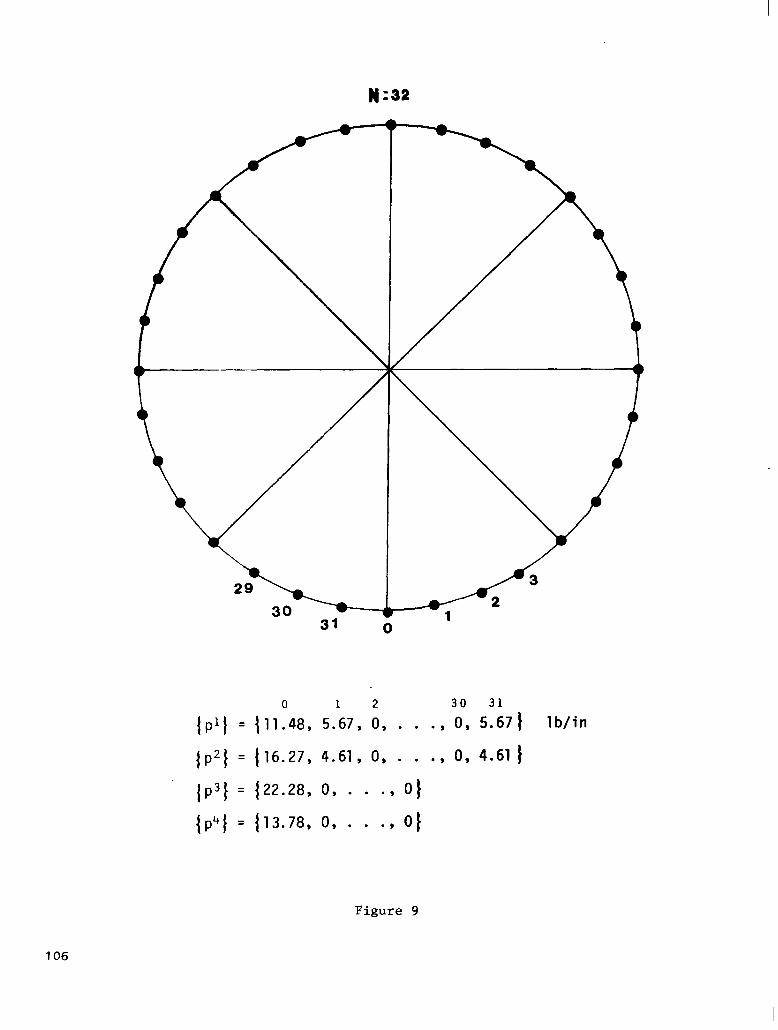
N:32

' ' * {pit = 1 11.48, 5.67, 0, . . ., y, 5yk7t lb/in

{p't = {16.27, 4.61, 0, . . ., 0, 4.61 t

lP3t = 1 22.28, 0, . . ., ot

(P4t = ( 13.78, 0, . . ., ot

Figure 9

106

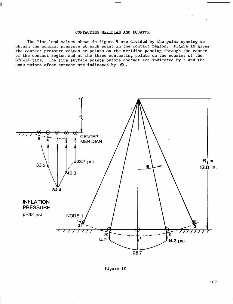
CONTACTING MERIDIAN AND EQUATOR

The line load values shown in figure 9 are divided by the point spacing to obtain the contact pressure at each point in the contact region. Figure 10 gives the contact pressure values at points on the meridian passing through the center of the contact region and at the three contacting points on the equator of the 678-14 tire. The tire surface points before contact are indicated by l and the same points after contact are indicated by 0 .

I MERIDIAN

28.7 psi

INFLATION PRESSURE p=32 psi

Figure 10

) in.

107

CONTACT PRESSURE DISTRIEUTION

All of the contact pressure values (psi) calculated for the G78-14 tire with 221 kPa (32psi) inflation pressure are shown in figure 11. The estimated location of the contact boundary is shown as a dashed oval. The contact boundary will be more accurately located when the density of points covered by the influence coeffi- cient matrix is increased. The point density is limited only by the size and speed of the computer used to execute the tire model program.

CONTACT BOUNDARY

Figure 11

108

AIRCRAFT TIRE SECTION

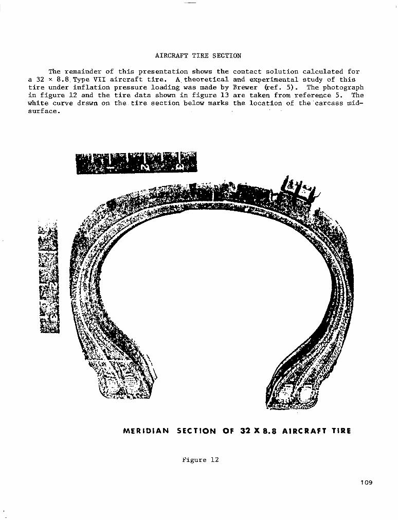
The remainder of this presentation shows the contact solution calculated for a 32 x 8.8.Type VII aircraft tire. A.theoretical and experimental study of this tire under inflation pressure loading was made by Erewer (ref. 5). The photograph in figure 12 and the tire data shown in figure 13 .are taken from reference 5. The white curve drawn on the tire section below marks the location of the'carcass mid- surface.

MERIDIAN SECTION OF 32 X 8.8 AIRCRAFT TIRE

Figure 12

109

MATERIAL PROPERTIES ANTI CARCASS GEOMETRY

The parameters shown in figure 13 are used in a preprocessing subroutine to calculate homogeneous orthotropic properties for the finite element tire model.

32 x 808 TYPE VII AIRCRAFT TIRE

Material Properties and Carcass Geometry

Rubber: ER = 450 psi, wR = 0.49, GR = 151 psi

Nylon Cord: EC = 156,000 psi, WC = 0.70, GC = 700 psi

Cord Diameter: dC = 0.031 in.

Ply Thickness: h = 0.043 in. (all plies)

Cord Angle B (measured from meridian) and Cord Density N, by Lift Formula ---.

Element B(deg) N(epi) Element $(deg) N(epi)

1 55.44 25.42 12 46.97 23.81

2 55.35 25.39 13 45.34 23.75

3 55.20 25.34 14 43.71 23.78

4 54.96 25.26 15 41.99 23.88

5 54.60 25.15 16 40.25 24.08

6 54.08 25.00 17 38.64 24.35

7 53.33 24.79 18 37.13 24.68

8 52.34 24.55 19 35.73 25.05

9 51.18 24.32 20 34.39 25.48

10 49.90 24.10 21 33.37 25.85

11 48.49 23.93

Construction: 6-ply, double bead

Figure 13

110

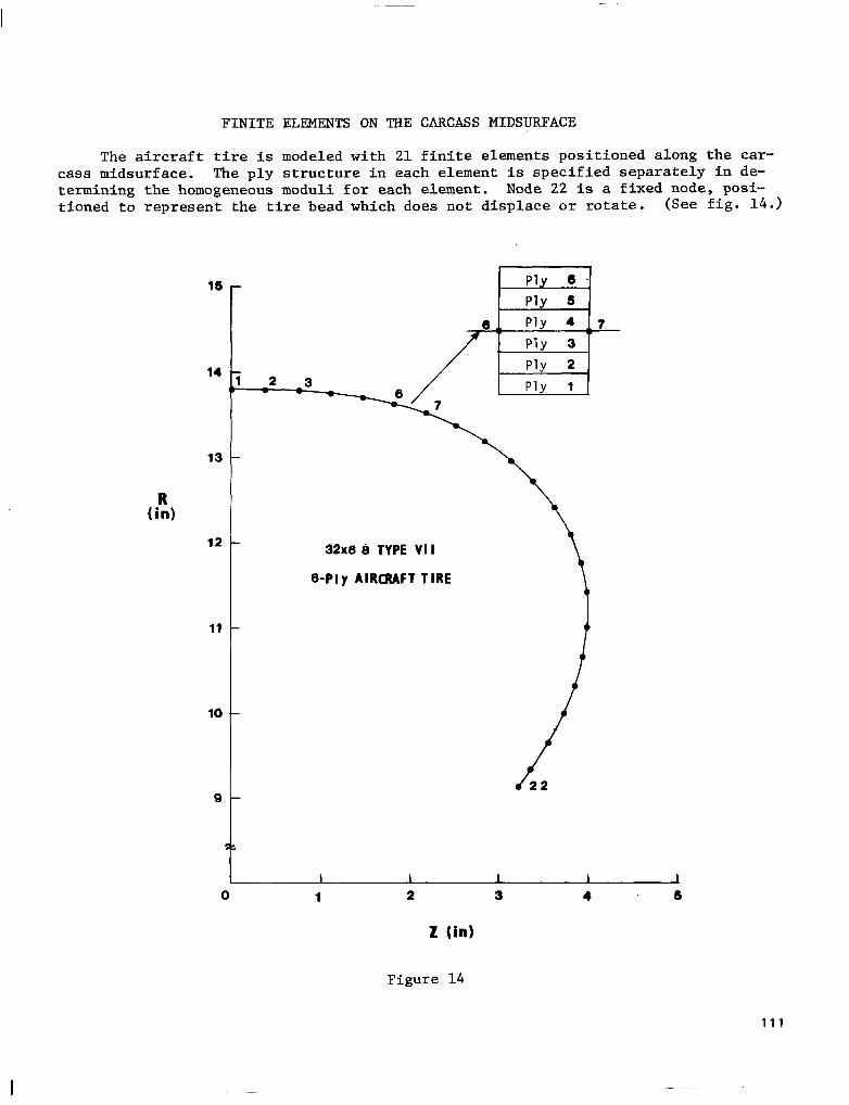
FINITE ELEMENTS ON THE CARCASS MIDSURFACE

The aircraft tire is modeled with 21 finite elements positioned along the car- cass midsurface. The ply structure in each element is specified separately in de- termining the homogeneous moduli for each element. Node 22 is a fixed node, posi- tioned to represent the tire bead which does not displace or rotate. (See fig. 14.)

15

14

13

12

11

10

Q

Ply 6

Ply 5

6.. Ply 4 ..7

i -2 3

32x8 b TYPE VII

6-Ply AIRCRAFT TIRE

0 1 2 3

L (in)

Figure 14

4 6

111

LOAD VECTOR CORRECTION DATA

The problem of calculating tire shape due to inflation pressure is highly nonlinear. As recognized by Stafford and Tabaddor (ref 6.), a successful solution can only be obtained by.a nonlinear finite element analysis which includes updating the pressure load vector direction during the inflation solution procedure. Table l-l, in figure 15, gives the input load vector components, pn and ps, that are needed in order to have the resultant pressure load normal to the inflated tire model.

CROWN

DEFORMED MERIDIAN

UNDEFORMED MERIDIAN

TABLE l-1. ~PUT LOAD DATA FOR FINITE ELEMENT MODEL OF AIRCRAFT TIRE ANALYZED BY BREWER

Element Rotation Number AO (de4

TIRELOAD' Input Pressure(psi)

P" ps

1 1.46 94.97 2.41 2 4.61 94.69 7.63 3 7.68 94.15 12.70 4 10.10 93.53 16.64 5 11.23 93.17 18.55 6 10.71 93.35 17.65 7 9.19 93.78 15.17 a 7.90 94.09 13.11 9 7.18 94.26 11.87

10 6.48 94.39 10.71 11 5.39 94.58 8.92 12 3.00 94.87 4.97 13 2.24 94.93 3.70 14 0 95.00 0

. .

21 6 95:oo 0

Figure 15

112

CROWN DISPLACEMENT VERSUS INFLATION PRESSURE

The effect of correcting the load vector is clearly seen in figure 16. The finite element solution obtained when the pressure direction remains normal to the undeformed elements is indicated by A's. The solution found when the pressure is normal to the deformed elements is indicated by X'S. This solution compares well with the calculation and measurements made by Brewer (ref. 5).

.7

.6

5

.4

.3

.2

.I

0

CROWN DISPLACEMENT (INCHES)

a n

a FINITE ELEMENT SOLUTION WITH Pn=95, Ps = 0

n A

BY

IO 40 50 60 70

INFLATION PRESSURE (psi)

80 90 100

Figure 16

113

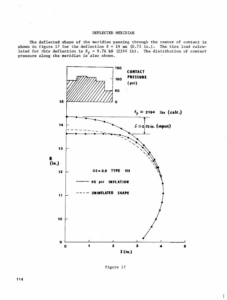
DEFLECTED MERIDIAN

The deflected shape of the meridian passirig through the center of contact is shown in figure 17 for the deflection 6 = 19 mm (0.75 in.). The tire load calcu- lated for this deflection is Fy = 9.76 kN (2194' lb). The distribution of contact pressure along the meridian is also shown.

15

13

R (in.)

12

11

10

9

-1 “’ CONTACT

100 PRESSURE

(Psi)

50

32 x 0.8 TYPE VII

95 psi INFLATION

---- UN INFLATED SHAPE

0 1 2 3 4 5

2 (in.)

Figure 17

114

DEFLECTED EQUATOR

The deflected shape of the equator and the distribution of, contact pressure along it are shown in figure 18. Since only three points on the equator lie in the contact region, only a rough estimate of the circumferential location of the contact boundary can be made.

.’ 32x8.8

/ I / I/

i

I I ‘\ \

Figure 18

115

TIRE LOAD VERSUS TIRE DEFLECTION

Calculated values of tire load for specified tire deflections are shown in figure 19.

6000

5000

TIRE

LOAD

4000

Fy (lb)

3000

2000

1000

0 0 0.25 0.50 0.75 1.00 1.25

32 x8.8 TYPE VII

AIRCRAFT TIRE / 95 psi INFLATION

TIRE DEFLECTIDN d (in)

Figure 19

116

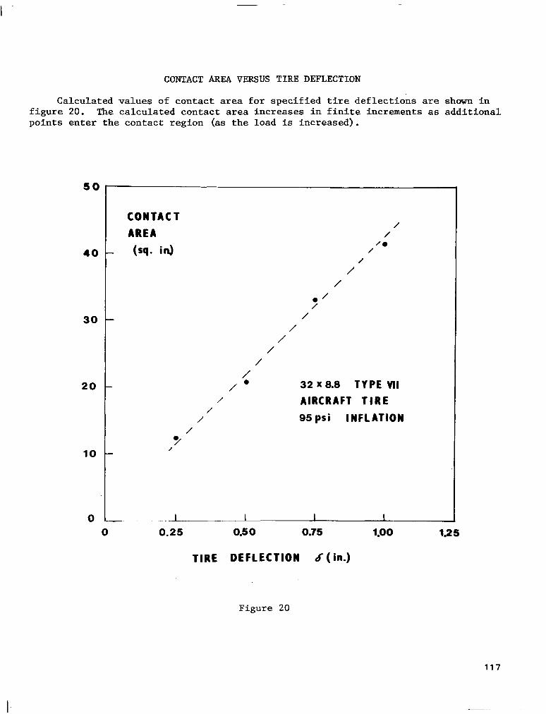
CONTACT AREA VERSUS TIRE DEFLECTION

Calculated values of contact area for specified tire deflections are shown in figure 20. The calculated contact area increases in finite increments as additional points enter the contact region (as the load is increased).

50

40

30

20

10

0 =

CONTACT AREA

(sq. id

/

/

/

/

“/ /

.L- 0.25

TIRE

/ /

10 /

/ /

/

7 / /

/ /

/ /

/ i 32 x 8.8 TYPE VII

AIRCRAFT TIRE 95 psi INFLATION

0.50 0.75

DEFLECTION d (in.)

1.00 195

Figure 20

117

All of the loads are shown

/ I’ I I

-/-- ------- -- 4- -+ 48.7 -\ 0 \

0 \ 90.5 \

\

21.3 105.6 21.3 ' \

34.4 108.6 34.4 I

I I I 28.3 90.7 psi 28.3 1

1 34.4 108.6 34.4 \ : \ 21.3 105.6 21.3

\ \ 90.5 /

\ / \ 49.7 /

. -- ,-/ -- --___---- ---

CALCULATED CONTACT PRESSURE DISTRIBUTIONS

contact pressure values (psi) calculated for two different tire in figure 21. The tire inflation pressure is 655 kPa (95 psi).

AIRCRAFT TIRE CONTACT PRESSURE DISTRIBUTIONS

(a) 6 = 0.75 in., Fz = 2200 lb

/----- --------------- -\ \

/ 0 .\ 12.9 130.4 12.9 \

\ 45.1 187.9 45.1 \

/ \ I 57.3 135.9 57.3 \

I

I 42.9 132.6 42.9

1

I 38.2 108.9 psi 38.2 I

\ 42.9 132.6 42.9 \ 57.3 135.9 57.3 :

\ \ 45.1 187.9 45.1

\ I \ 12.9 130.4 12.9 \

HR

,/

. ------ ----_--------- --

(b) 6 = 1.00 in., Fz = 3700 lb

Figure 21

118

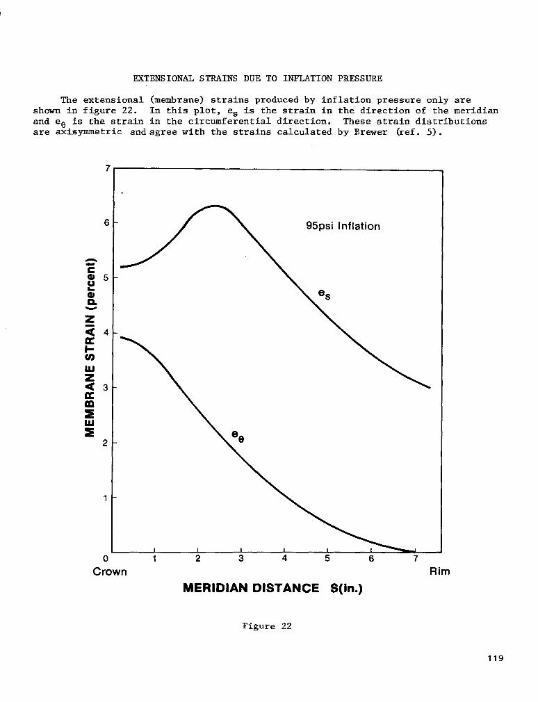
EXTENSIONAL STRAINS DUE TO INFLATION PRESSURE

The extensional (membrane) strains produced by inflation pressure only are shown in figure 22. In this plot, es is the strain in the direction of the meridian and ee is the strain in the circumferential direction. These strain distributions are axisymmetric andagree with the strains calculated by Brewer (ref. 5).

Crown Rim

MERIDIAN DISTANCE S(in.)

Figure 22

119

FORCE RESULTANTS DUE TO INFLATION PRESSURE

The membrane forces (per unit length) produced by inflation pressure only are shown in figure 23. The forces N, and N0 are in the meridional and circumferential directions, respectively. These force distributions are axisymmetric.

600

500

E- T g 400

i!i

5 LL 300

s

2

ii 200

100

0

95 psi Inflation

I I I I 1 I I

1 2 3 4 5 6 7

Crown Rim MERIDIAN DISTANCE S(in.)

Figure 23

120

REFERENCES

1. Tillerson, J. R.; and Haisler, W. E.: SAMMSOR II - A Finite Element Program to Determine Stiffness and Mass Matrices of Shells of Revolution. TEES-RPT-70-18, Texas A&M University, Oct. 1970.

2. Haisler, W. E.; and Stricklin, J. A.: SNASOR II - A Finite Element Program for the Static Nonlinear Analysis of Shells of Revolution. TEES-RPT-70-20, Texas A&M University, Oct. 1970.

3. Schapery, R. A.; and Tielking, J. T.: Investigation of Tire-Pavement Interac- tion During Maneuvering: Theory and Results. Report No. FHWA-RD-78-72, Federal Highway Administration, June 1977.

4. Tielking, J. T.; and Schapery, R. A.: A Method for Shell Contact Analysis. Computer Methods in Applied Mechanics and Engineering, Vol. 26, NO. 2, pp. 181-195, May 1981.

5. Erewer, H. K.: Stresses and Deformations in Multi-Ply Aircraft Tires Subject to Inflation Pressure Loading. Report No. AFFDL-TR-70-62, Air Force Flight Dynamics Laboratory, June 1970.

6. Stafford, J. R.; and Tabaddor, F.: ADINA Load Updating for Pressurized Struc- tures. Symposium on Finite Element Analysis of Tires, ASTM F-9, May 1980.

121