Embed Size (px)
Citation preview
arX
iv:1
003.
4485
v2 [
hep-
th]
18
Feb
2015
An Invitation to Higher Gauge Theory
John C. Baez and John Huerta
Department of Mathematics, University of California
Riverside, California 92521
USA
email: [email protected] [email protected]
March 24, 2010
Abstract
In this easy introduction to higher gauge theory, we describe parallel trans-port for particles and strings in terms of 2-connections on 2-bundles. Justas ordinary gauge theory involves a gauge group, this generalization in-volves a gauge ‘2-group’. We focus on 6 examples. First, every abelianLie group gives a Lie 2-group; the case of U(1) yields the theory of U(1)gerbes, which play an important role in string theory and multisymplec-tic geometry. Second, every group representation gives a Lie 2-group; therepresentation of the Lorentz group on 4d Minkowski spacetime gives thePoincare 2-group, which leads to a spin foam model for Minkowski space-time. Third, taking the adjoint representation of any Lie group on its ownLie algebra gives a ‘tangent 2-group’, which serves as a gauge 2-group in4d BF theory, which has topological gravity as a special case. Fourth,every Lie group has an ‘inner automorphism 2-group’, which serves as thegauge group in 4d BF theory with cosmological constant term. Fifth, ev-ery Lie group has an ‘automorphism 2-group’, which plays an importantrole in the theory of nonabelian gerbes. And sixth, every compact simpleLie group gives a ‘string 2-group’. We also touch upon higher structuressuch as the ‘gravity 3-group’, and the Lie 3-superalgebra that governs11-dimensional supergravity.
1 Introduction
Higher gauge theory is a generalization of gauge theory that describes paralleltransport, not just for point particles, but also for higher-dimensional extendedobjects. It is a beautiful new branch of mathematics, with a lot of room leftfor exploration. It has already been applied to string theory and loop quantumgravity—or more specifically, spin foam models. This should not be surprising,since while these rival approaches to quantum gravity disagree about almost
1
everything, they both agree that point particles are not enough: we need higher-dimensional extended objects to build a theory sufficiently rich to describe thequantum geometry of spacetime. Indeed, many existing ideas from string theoryand supergravity have recently been clarified by higher gauge theory [82, 83].But we may also hope for applications of higher gauge theory to other lessspeculative branches of physics, such as condensed matter physics.
Of course, for this to happen, more physicists need to learn higher gaugetheory. It would be great to have a comprehensive introduction to the subjectwhich started from scratch and led the reader to the frontiers of knowledge. Un-fortunately, mathematical work in this subject uses a wide array of tools, such asn-categories, stacks, gerbes, Deligne cohomology, L∞ algebras, Kan complexes,and (∞, 1)-categories, to name just a few. While these tools are beautiful, im-portant in their own right, and perhaps necessary for a deep understanding ofhigher gauge theory, learning them takes time—and explaining them all wouldbe a major project.
Our goal here is far more modest. We shall sketch how to generalize thetheory of parallel transport from point particles to 1-dimensional objects, suchas strings. We shall do this starting with a bare minimum of prerequisites:manifolds, differential forms, Lie groups, Lie algebras, and the traditional theoryof parallel transport in terms of bundles and connections. We shall give a smalltaste of the applications to physics, and point the reader to the literature formore details.
In Section 2 we start by explaining categories, functors, and how paralleltransport for particles can be seen as a functor taking any path in a manifoldto the operation of parallel transport along that path. In Section 3 we ‘addone’ and explain how parallel transport for particles and strings can be seen as‘2-functor’ between ‘2-categories’. This requires that we generalize Lie groupsto ‘Lie 2-groups’. In Section 4 we describe many examples of Lie 2-groups, andsketch some of their applications:
• Section 4.1: shifted abelian groups, U(1) gerbes, and their role in stringtheory and multisymplectic geometry.
• Section 4.2: the Poincare 2-group and the spin foammodel for 4d Minkowskispacetime.
• Section 4.3: tangent 2-groups, 4d BF theory and topological gravity.
• Section 4.4: inner automorphism 2-groups and 4d BF theory with cosmo-logical constant term.
• Section 4.5: automorphism 2-groups, nonabelian gerbes, and the gravity3-group.
• Section 4.6: string 2-groups, string structures, the passage from Lie n-algebras to Lie n-groups, and the Lie 3-superalgebra governing 11-dimensionalsupergravity.
2
Finally, in Section 5 we discuss gauge transformations, curvature and nontrivial2-bundles.
2 Categories and Connections
A category consists of objects, which we draw as dots:
• x
and morphisms between objects, which we draw as arrows between dots:
x•
f
''•y
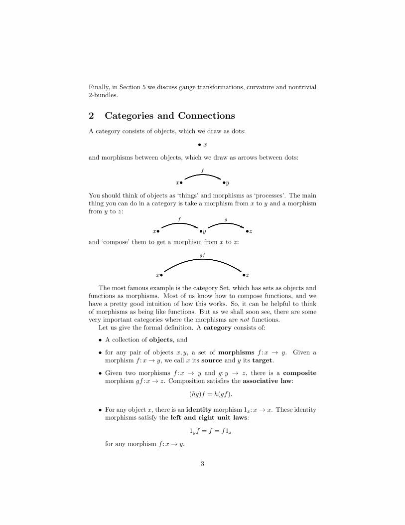
You should think of objects as ‘things’ and morphisms as ‘processes’. The mainthing you can do in a category is take a morphism from x to y and a morphismfrom y to z:
x•
f
''•y
g
''•z
and ‘compose’ them to get a morphism from x to z:
x•
gf
$$•z
The most famous example is the category Set, which has sets as objects andfunctions as morphisms. Most of us know how to compose functions, and wehave a pretty good intuition of how this works. So, it can be helpful to thinkof morphisms as being like functions. But as we shall soon see, there are somevery important categories where the morphisms are not functions.
Let us give the formal definition. A category consists of:
• A collection of objects, and
• for any pair of objects x, y, a set of morphisms f :x → y. Given amorphism f :x → y, we call x its source and y its target.
• Given two morphisms f :x → y and g: y → z, there is a compositemorphism gf :x → z. Composition satisfies the associative law:
(hg)f = h(gf).
• For any object x, there is an identitymorphism 1x:x → x. These identitymorphisms satisfy the left and right unit laws:
1yf = f = f1x
for any morphism f :x → y.
3
The hardest thing about category theory is getting your arrows to point theright way. It is standard in mathematics to use fg to denote the result of doingfirst g and then f . In pictures, this backwards convention can be annoying. Butrather than trying to fight it, let us give in and draw a morphism f :x → y asan arrow from right to left:
y• •x
f
ww
Then composition looks a bit better:
z• •y
f
ww•x
g
ww= z• •x
fg
ww
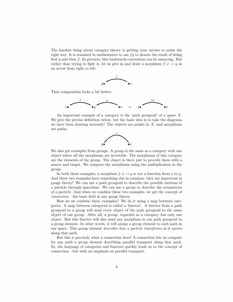
An important example of a category is the ‘path groupoid’ of a space X .We give the precise definition below, but the basic idea is to take the diagramswe have been drawing seriously! The objects are points in X , and morphismsare paths:
y• •x
γ
We also get examples from groups. A group is the same as a category with oneobject where all the morphisms are invertible. The morphisms of this categoryare the elements of the group. The object is there just to provide them with asource and target. We compose the morphisms using the multiplication in thegroup.
In both these examples, a morphism f :x → y is not a function from x to y.And these two examples have something else in common: they are important ingauge theory! We can use a path groupoid to describe the possible motions ofa particle through spacetime. We can use a group to describe the symmetriesof a particle. And when we combine these two examples, we get the concept ofconnection—the basic field in any gauge theory.
How do we combine these examples? We do it using a map between cate-gories. A map between categories is called a ‘functor’. A functor from a pathgroupoid to a group will send every object of the path groupoid to the sameobject of our group. After all, a group, regarded as a category, has only oneobject. But this functor will also send any morphism in our path groupoid toa group element. In other words, it will assign a group element to each path inour space. This group element describes how a particle transforms as it movesalong that path.
But this is precisely what a connection does! A connection lets us computefor any path a group element describing parallel transport along that path.So, the language of categories and functors quickly leads us to the concept ofconnection—but with an emphasis on parallel transport.
4
The following theorem makes these ideas precise. Let us first state thetheorem, then define the terms involved, and then give some idea of how it isproved:
Theorem 1. For any Lie group G and any smooth manifold M , there is a
one-to-one correspondence between:
1. connections on the trivial principal G-bundle over M ,
2. g-valued 1-forms on M , where g is the Lie algebra of G, and
3. smooth functors
hol:P1(M) → G
where P1(M) is the path groupoid of M .
We assume you are familiar with the first two items. Our goal is to explain thethird. We must start by explaining the path groupoid.
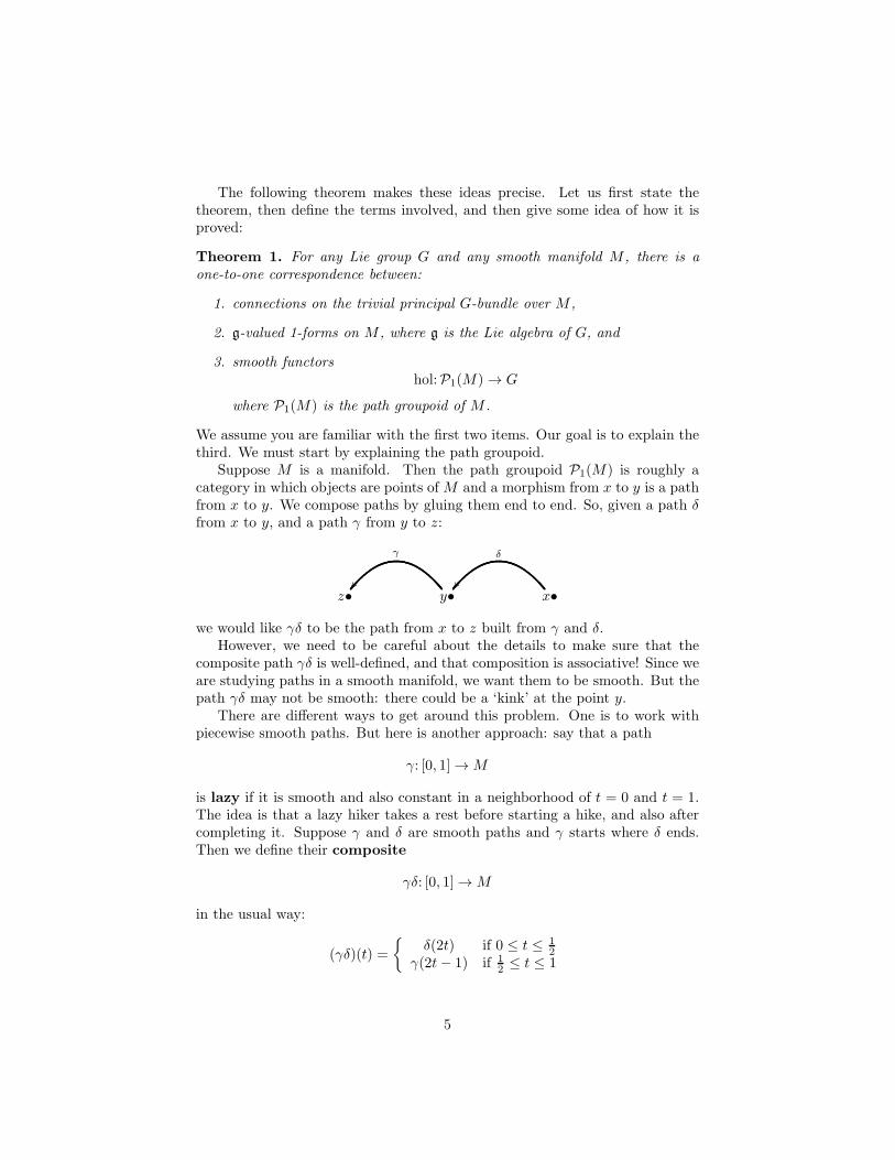
Suppose M is a manifold. Then the path groupoid P1(M) is roughly acategory in which objects are points of M and a morphism from x to y is a pathfrom x to y. We compose paths by gluing them end to end. So, given a path δfrom x to y, and a path γ from y to z:
z• y•
γ
x•
δ
we would like γδ to be the path from x to z built from γ and δ.However, we need to be careful about the details to make sure that the
composite path γδ is well-defined, and that composition is associative! Since weare studying paths in a smooth manifold, we want them to be smooth. But thepath γδ may not be smooth: there could be a ‘kink’ at the point y.
There are different ways to get around this problem. One is to work withpiecewise smooth paths. But here is another approach: say that a path
γ: [0, 1] → M
is lazy if it is smooth and also constant in a neighborhood of t = 0 and t = 1.The idea is that a lazy hiker takes a rest before starting a hike, and also aftercompleting it. Suppose γ and δ are smooth paths and γ starts where δ ends.Then we define their composite
γδ: [0, 1] → M
in the usual way:
(γδ)(t) =
δ(2t) if 0 ≤ t ≤ 12
γ(2t− 1) if 12 ≤ t ≤ 1
5
In other words, γδ spends the first half of its time moving along δ, and thesecond half moving along γ. In general the path γδ may not be smooth att = 1
2 . However, if γ and δ are lazy, then their composite is smooth—and it,too, is lazy!
So, lazy paths are closed under composition. Unfortunately, composition oflazy paths is not associative. The paths (αβ)γ and α(βγ) differ by a smoothreparametrization, but they are not equal. To solve this problem, we can takecertain equivalence classes of lazy paths as morphisms in the path groupoid.
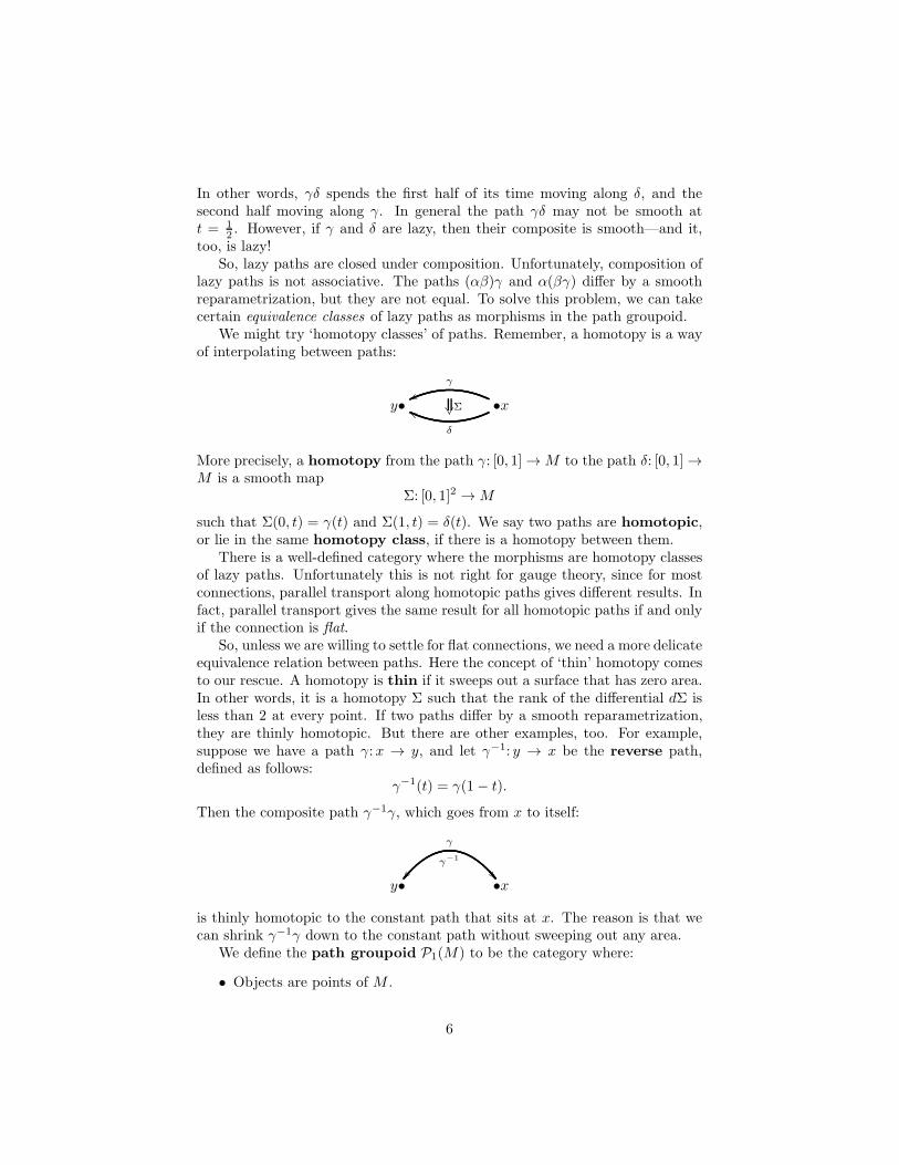
We might try ‘homotopy classes’ of paths. Remember, a homotopy is a wayof interpolating between paths:
y• •x
δ
gg
γ
wwΣ
More precisely, a homotopy from the path γ: [0, 1] → M to the path δ: [0, 1] →M is a smooth map
Σ: [0, 1]2 → M
such that Σ(0, t) = γ(t) and Σ(1, t) = δ(t). We say two paths are homotopic,or lie in the same homotopy class, if there is a homotopy between them.
There is a well-defined category where the morphisms are homotopy classesof lazy paths. Unfortunately this is not right for gauge theory, since for mostconnections, parallel transport along homotopic paths gives different results. Infact, parallel transport gives the same result for all homotopic paths if and onlyif the connection is flat.
So, unless we are willing to settle for flat connections, we need a more delicateequivalence relation between paths. Here the concept of ‘thin’ homotopy comesto our rescue. A homotopy is thin if it sweeps out a surface that has zero area.In other words, it is a homotopy Σ such that the rank of the differential dΣ isless than 2 at every point. If two paths differ by a smooth reparametrization,they are thinly homotopic. But there are other examples, too. For example,suppose we have a path γ:x → y, and let γ−1: y → x be the reverse path,defined as follows:
γ−1(t) = γ(1− t).
Then the composite path γ−1γ, which goes from x to itself:
y• •x
γ−1
γ
is thinly homotopic to the constant path that sits at x. The reason is that wecan shrink γ−1γ down to the constant path without sweeping out any area.
We define the path groupoid P1(M) to be the category where:
• Objects are points of M .
6
• Morphisms are thin homotopy classes of lazy paths in M .
• If we write [γ] to denote the thin homotopy class of the path γ, compositionis defined by
[γ][δ] = [γδ].
• For any point x ∈ M , the identity 1x is the thin homotopy class of theconstant path at x.
With these rules, it is easy to check that P1(M) is a category. The mostimportant point is that since the composite paths (αβ)γ and α(βγ) differ by asmooth reparametrization, they are thinly homotopic. This gives the associativelaw when we work with thin homotopy classes.
But as its name suggests, P1(M) is better than a mere category. It is agroupoid: that is, a category where every morphism γ:x → y has an inverseγ−1: y → x satisfying
γ−1γ = 1x and γγ−1 = 1y
In P1(M), the inverse is defined using the concept of a reverse path:
[γ]−1 = [γ−1].
The rules for an inverse only hold in P1(M) after we take thin homotopy classes.After all, the composites γγ−1 and γ−1γ are not constant paths, but they arethinly homotopic to constant paths. But henceforth, we will relax and writesimply γ for the morphism in the path groupoid corresponding to a path γ,instead of [γ].
As the name suggests, groupoids are a bit like groups. Indeed, a group issecretly the same as a groupoid with one object! In other words, suppose wehave group G. Then there is a category where:
• There is only one object, •.
• Morphisms from • to • are elements of G.
• Composition of morphisms is multiplication in the group G.
• The identity morphism 1• is the identity element of G.
This category is a groupoid, since every group element has an inverse. Con-versely, any groupoid with one object gives a group. Henceforth we will freelyswitch back and forth between thinking of a group in the traditional way, andthinking of it as a one-object groupoid.
How can we use groupoids to describe connections? It should not be sur-prising that we can do this, now that we have our path groupoid P1(M) andour one-object groupoid G in hand. A connection gives a map from P1(M) toG, which says how to transform a particle when we move it along a path. Moreprecisely: if G is a Lie group, any connection on the trivial G-bundle over M
7
yields a map, called the parallel transport map or holonomy, that assigns anelement of G to each path:
hol: • •
γvv
7→ hol(γ) ∈ G
In physics notation, the holonomy is defined as the path-ordered exponential ofsome g-valued 1-form A, where g is the Lie algebra of G:
hol(γ) = P exp
(∫
γ
A
)
∈ G.
The holonomy map satisfies certain rules, most of which are summarized inthe word ‘functor’. What is a functor? It is a map between categories thatpreserves all the structure in sight!
More precisely: given categories C and D, a functor F :C → D consists of:
• a map F sending objects in C to objects in D, and
• another map, also called F , sending morphisms in C to morphisms in D,
such that:
• given a morphism f :x → y in C, we have F (f):F (x) → F (y),
• F preserves composition:
F (fg) = F (f)F (g)
when either side is well-defined, and
• F preserves identities:F (1x) = 1F (x)
for every object x of C.
The last property actually follows from the rest. The second to last—preservingcomposition—is the most important property of functors. As a test of yourunderstanding, check that if C and D are just groups (that is, one-objectgroupoids) then a functor F :C → D is just a homomorphism.
Let us see what this definition says about a functor
hol:P1(M) → G
where G is some Lie group. This functor hol must send all the points of M tothe one object of G. More interestingly, it must send thin homotopy classes ofpaths in M to elements of G:
hol: • •
γvv
7→ hol(γ) ∈ G
8
It must preserve composition:
hol(γδ) = hol(γ) hol(δ)
and identities:hol(1x) = 1 ∈ G.
While they may be stated in unfamiliar language, these are actually well-known properties of connections! First, the holonomy of a connection along apath
hol(γ) = P exp
(∫
γ
A
)
∈ G
only depends on the thin homotopy class of γ. To see this, compute the variationof hol(γ) as we vary the path γ, and show the variation is zero if the homotopyis thin. Second, to compute the group element for a composite of paths, we justmultiply the group elements for each one:
P exp
(∫
γδ
A
)
= P exp
(∫
γ
A
)
P exp
(∫
δ
A
)
And third, the path-ordered exponential along a constant path is just the iden-tity:
P exp
(∫
1x
A
)
= 1 ∈ G.
All this information is neatly captured by saying hol is a functor. AndTheorem 1 says this is almost all there is to being a connection. The onlyadditional condition required is that hol be smooth. This means, roughly, thathol(γ) depends smoothly on the path γ—more on that later. But if we drop thiscondition, we can generalize the concept of connection, and define a generalizedconnection on a smooth manifold M to be a functor hol:P1(M) → G.
Generalized connections have long played an important role in loop quan-tum gravity, first in the context of real-analytic manifolds [3], and later forsmooth manifolds [17, 65]. The reason is that if M is any manifold and Gis a connected compact Lie group, there is a natural measure on the space ofgeneralized connections. This means that you can define a Hilbert space ofcomplex-valued square-integrable functions on the space of generalized connec-tions. In loop quantum gravity these are used to describe quantum states beforeany constraints have been imposed. The switch from connections to generalizedconnections is crucial here—and the lack of smoothness gives loop quantumgravity its ‘discrete’ flavor.
But suppose we are interested in ordinary connections. Then we really wanthol(γ) to depend smoothly on the path γ. How can we make this precise?
One way is to use the theory of ‘smooth groupoids’ [16]. Any Lie groupis a smooth groupoid, and so is the path groupoid of any smooth manifold.We can define smooth functors between smooth groupoids, and then smoothfunctors hol:P1(M) → G are in one-to-one correspondence with connections on
9
the trivial principal G-bundle over M . We can go even further: there are moregeneral maps between smooth groupoids, and maps hol:P1(M) → G of thismore general sort correspond to connections on not necessarily trivial principalG-bundles over M . For details, see the work of Bartels [25], Schreiber andWaldorf [87].
But if this sounds like too much work, we can take the following shortcut.Suppose we have a smooth function F : [0, 1]n × [0, 1] → M , which we think ofas a parametrized family of paths. And suppose that for each fixed value of theparameter s ∈ [0, 1]n, the path γs given by
γs(t) = F (s, t)
is lazy. Then our functor hol:P1(M) → G gives a function
[0, 1]n → Gs 7→ hol(γs).
If this function is smooth whenever F has the above properties, then the functorhol:P1(M) → G is smooth.
Starting from this definition one can prove the following lemma, which liesat the heart of Theorem 1:
Lemma. There is a one-to-one correspondence between smooth functors
hol:P1(M) → G and Lie(G)-valued 1-forms A on M .
The idea is that given a Lie(G)-valued 1-form A on M , we can define aholonomy for any smooth path as follows:
hol(γ) = P exp
(∫
γ
A
)
,
and then check that this defines a smooth functor hol:P1(M) → G. Conversely,suppose we have a smooth functor hol of this sort. Then we can define hol(γ)for smooth paths γ that are not lazy, using the fact that every smooth path isthinly homotopic to a lazy one. We can even do this for paths γ: [0, s] → Mwhere s 6= 1, since any such path can be reparametrized to give a path of theusual sort. Given a smooth path
γ: [0, 1] → M
we can truncate it to obtain a path γs that goes along γ until time s:
γs: [0, s] → M.
By what we have said, hol(γs) is well-defined. Using the fact that hol:P1(M) →G is a smooth functor, one can check that hol(γs) varies smoothly with s. So,we can differentiate it and define a Lie(G)-valued 1-form A as follows:
A(v) =d
dshol(γs)
∣
∣
s=0
10
where v is any tangent vector at a point x ∈ M , and γ is any smooth path with
γ(0) = x, γ′(0) = v.
Of course, we need to check that A is well-defined and smooth. We also need tocheck that if we start with a smooth functor hol, construct a 1-form A in thisway, and then turn A back into a smooth functor, we wind up back where westarted.
3 2-Categories and 2-Connections
Now we want to climb up one dimension, and talk about ‘2-connections’. Aconnection tells us how particles transform as they move along paths. A 2-connection will also tell us how strings transform as they sweep out surfaces. Tomake this idea precise, we need to take everything we said in the previous sectionand boost the dimension by one. Instead of categories, we need ‘2-categories’.Instead of groups, we need ‘2-groups’. Instead of the path groupoid, we needthe ‘path 2-groupoid’. And instead of functors, we need ‘2-functors’. Whenwe understand all these things, the analogue of Theorem 1 will look strikinglysimilar to the original version:
Theorem. For any Lie 2-group G and any smooth manifold M , there is a
one-to-one correspondence between:
1. 2-connections on the trivial principal G-2-bundle over M ,
2. pairs consisting of a smooth g-valued 1-form A and a smooth h-valued
2-form B on M , such that
t(B) = dA+A ∧A
where we use t: h → g, the differential of the map t:H → G, to convert Binto a g-valued 2-form, and
3. smooth 2-functors
hol:P2(M) → G
where P2(M) is the path 2-groupoid of M .
What does this say? In brief: there is a way to extract from a Lie 2-groupG a pair of Lie groups G and H . Suppose we have a 1-form A taking values inthe Lie algebra of G, and a 2-form B valued in the Lie algebra of H . Supposefurthermore that these forms obey the equation above. Then we can use themto consistently define parallel transport, or ‘holonomies’, for paths and surfaces.They thus define a ‘2-connection’.
That is the idea. But to make it precise, we need 2-categories.
11
3.1 2-Categories
Sets have elements. Categories have elements, usually called ‘objects’, but alsomorphisms between these. In an ‘n-category’, we go further and include 2-morphisms between morphisms, 3-morphisms between 2-morphisms,... and soon up to the nth level. We are beginning to see n-categories provide an algebraiclanguage for n-dimensional structures in physics [12]. Higher gauge theory isjust one place where this is happening.
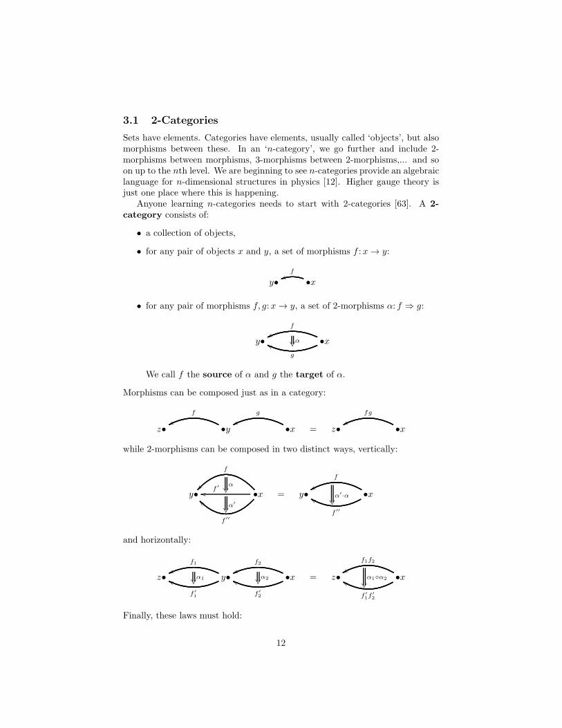
Anyone learning n-categories needs to start with 2-categories [63]. A 2-category consists of:
• a collection of objects,
• for any pair of objects x and y, a set of morphisms f :x → y:
y• •x
fuu
• for any pair of morphisms f, g:x → y, a set of 2-morphisms α: f ⇒ g:
y• •x
g
gg
f
wwα
We call f the source of α and g the target of α.
Morphisms can be composed just as in a category:
z• •y
f
ww•x
g
ww= z• •x
fg
ww
while 2-morphisms can be composed in two distinct ways, vertically:
y• •x
f
f ′
oo
f ′′
``
α
α′
= y• •x
f
xx
f ′′
ff α′·α
and horizontally:
z• y•
f1
vv
f ′
1
hh α1 •x
f2
ww
f ′
2
gg α2 = z• •x
f1f2
xx
f ′
1f′
2
ff α1α2
Finally, these laws must hold:
12
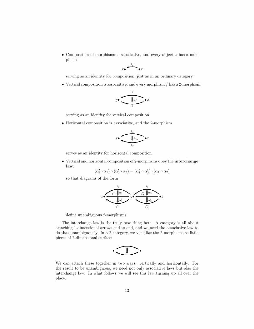
• Composition of morphisms is associative, and every object x has a mor-phism
x• •x1xuu
serving as an identity for composition, just as in an ordinary category.
• Vertical composition is associative, and every morphism f has a 2-morphism
y• •x
f
gg
f
ww1f
serving as an identity for vertical composition.
• Horizontal composition is associative, and the 2-morphism
x• •x
1x
hh
1x
vv11x
serves as an identity for horizontal composition.
• Vertical and horizontal composition of 2-morphisms obey the interchangelaw:
(α′
1 · α1) (α′
2 · α2) = (α′
1 α′
2) · (α1 α2)
so that diagrams of the form
x• y•
f1
|| f ′
1oo
f ′′
1
bbα1α′
1•z
f2
|| f ′
2oo
f ′′
2
cc
α2α′
2
define unambiguous 2-morphisms.
The interchange law is the truly new thing here. A category is all aboutattaching 1-dimensional arrows end to end, and we need the associative law todo that unambiguously. In a 2-category, we visualize the 2-morphisms as littlepieces of 2-dimensional surface:
• •ffxx
We can attach these together in two ways: vertically and horizontally. Forthe result to be unambiguous, we need not only associative laws but also theinterchange law. In what follows we will see this law turning up all over theplace.
13
3.2 Path 2-Groupoids
Path groupoids play a big though often neglected role in physics: the pathgroupoid of a spacetime manifold describes all the possible motions of a pointparticle in that spacetime. The path 2-groupoid does the same thing for particlesand strings.
First of all, a 2-groupoid is a 2-category where:
• Every morphism f :x → y has an inverse, f−1: y → x, such that:
f−1f = 1x and ff−1 = 1y.
• Every 2-morphism α: f ⇒ g has a vertical inverse, α−1vert: g ⇒ f , such
that:α−1vert · α = 1f and α · α−1
vert = 1f .
It actually follows from this definition that every 2-morphism α: f ⇒ g also hasa horizontal inverse, α−1
hor: f−1 ⇒ g−1, such that:
α−1
hor α = 11x and α α−1
hor = 11x .
So, a 2-groupoid has every kind of inverse your heart could desire.An example of a 2-group is the ‘path 2-groupoid’ of a smooth manifold M .
To define this, we can start with the path groupoid P1(M) as defined in theprevious section, and then throw in 2-morphisms. Just as the morphisms inP1(M) were thin homotopy classes of lazy paths, these 2-morphisms will bethin homotopy classes of lazy surfaces.
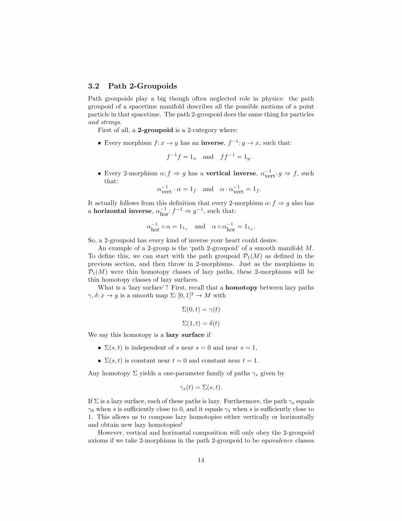
What is a ‘lazy surface’? First, recall that a homotopy between lazy pathsγ, δ:x → y is a smooth map Σ: [0, 1]2 → M with
Σ(0, t) = γ(t)
Σ(1, t) = δ(t)
We say this homotopy is a lazy surface if
• Σ(s, t) is independent of s near s = 0 and near s = 1,
• Σ(s, t) is constant near t = 0 and constant near t = 1.
Any homotopy Σ yields a one-parameter family of paths γs given by
γs(t) = Σ(s, t).
If Σ is a lazy surface, each of these paths is lazy. Furthermore, the path γs equalsγ0 when s is sufficiently close to 0, and it equals γ1 when s is sufficiently close to1. This allows us to compose lazy homotopies either vertically or horizontallyand obtain new lazy homotopies!
However, vertical and horizontal composition will only obey the 2-groupoidaxioms if we take 2-morphisms in the path 2-groupoid to be equivalence classes
14
of lazy surfaces. We saw this kind of issue already when discussing the pathgroupoid, so we we will allow ourselves to be a bit sketchy this time. Thekey idea is to define a concept of ‘thin homotopy’ between lazy surfaces Σand Ξ. For starters, this should be a smooth map H : [0, 1]3 → M such thatH(0, s, t) = Σ(s, t) and H(1, s, t) = Ξ(s, t). But we also want H to be ‘thin’.In other words, it should sweep out no volume: the rank of the differential dHshould be less than 3 at every point.
To make thin homotopies well-defined between thin homotopy classes ofpaths, some more technical conditions are also useful. For these, the reader canturn to Section 2.1 of Schreiber and Waldorf [87]. The upshot is that we obtainfor any smooth manifold M a path 2-groupoid P2(M), in which:
• An object is a point of M .
• A morphism from x to y is a thin homotopy class of lazy paths from x toy.
• A 2-morphism between equivalence classes of lazy paths γ0, γ1:x → y is athin homotopy class of lazy surfaces Σ: γ0 ⇒ γ1.
As we already did with the concept of ‘lazy path’, we will often use ‘lazy surface’to mean a thin homotopy class of lazy surfaces. But now let us hasten on toanother important class of 2-groupoids, the ‘2-groups’. Just as groups describesymmetries in gauge theory, these describe symmetries in higher gauge theory.
3.3 2-Groups
Just as a group was a groupoid with one object, we define a 2-group to be a2-groupoid with one object. This definition is so elegant that it may be hard tounderstand at first! So, it will be useful to take a 2-group G and chop it intofour bite-sized pieces of data, giving a ‘crossed module’ (G,H, t, α). Indeed, 2-groups were originally introduced in the guise of crossed modules by the famoustopologist J. H. C. Whitehead [93]. In 1950, with help from Mac Lane [66], heused crossed modules to generalize the fundamental group of a space to whatwe might now call the ‘fundamental 2-group’. But only later did it become clearthat a crossed module was another way of talking about a 2-groupoid with justone object! For more of this history, and much more on 2-groups, see [13].
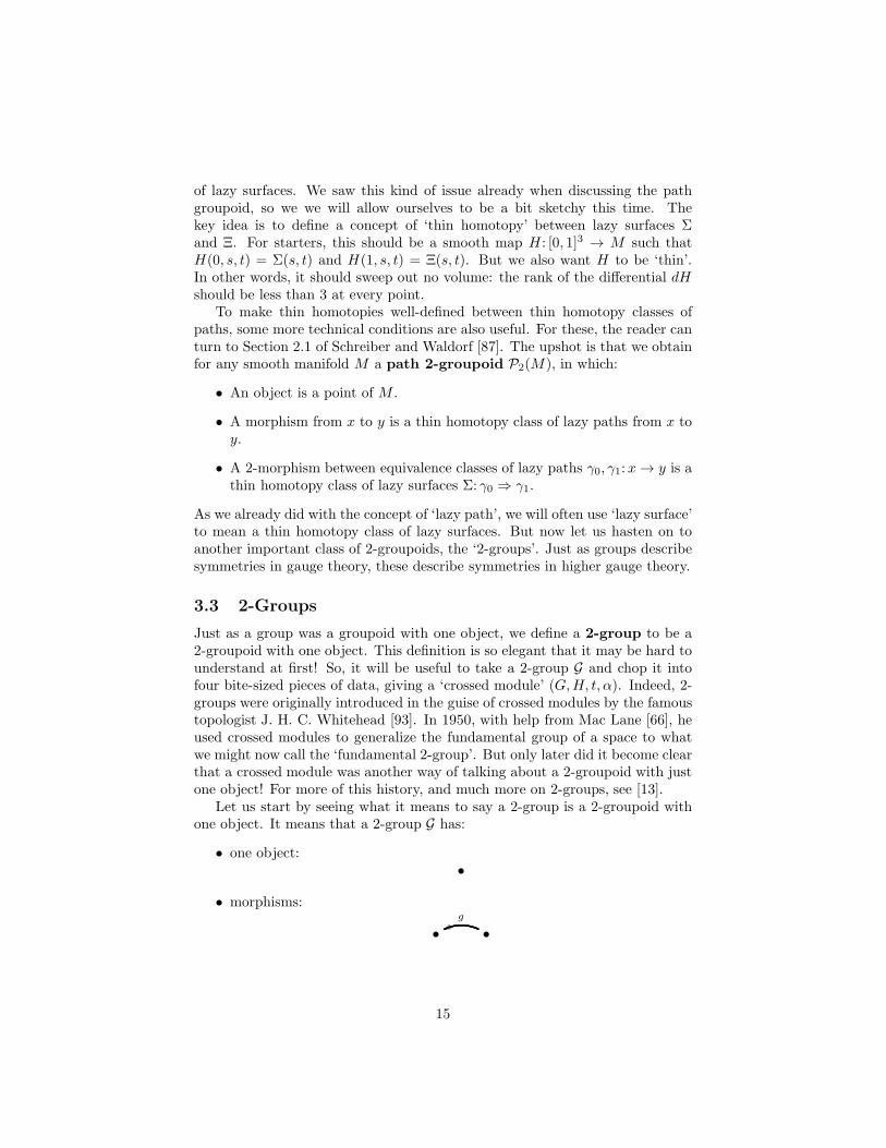
Let us start by seeing what it means to say a 2-group is a 2-groupoid withone object. It means that a 2-group G has:
• one object:•
• morphisms:
• •
gvv
15
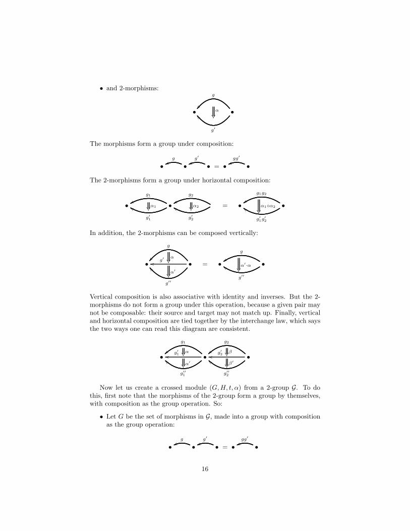
• and 2-morphisms:
• •
g
g′
\\α
The morphisms form a group under composition:
• •
gvv
•
g′
vv= • •
gg′
vv
The 2-morphisms form a group under horizontal composition:
• •
g1
xx
g′
1
ff α1
g2
xx
g′
2
ff α2 = • •
g1g2
zz
g′
1g′
2
dd α1α2
In addition, the 2-morphisms can be composed vertically:
• •
g
g′
oo
g′′
]]
α
α′
= • •
g
zz
g′′
dd α′·α
Vertical composition is also associative with identity and inverses. But the 2-morphisms do not form a group under this operation, because a given pair maynot be composable: their source and target may not match up. Finally, verticaland horizontal composition are tied together by the interchange law, which saysthe two ways one can read this diagram are consistent.
• •
g1
g′
1oo
g′′
1
aaα
α′
•
g2
g′
2oo
g′′
2
aaββ′
Now let us create a crossed module (G,H, t, α) from a 2-group G. To dothis, first note that the morphisms of the 2-group form a group by themselves,with composition as the group operation. So:
• Let G be the set of morphisms in G, made into a group with compositionas the group operation:
• •g
vv•
g′
vv= • •
gg′
vv
16
How about the 2-morphisms? These also form a group, with horizontal com-position as the group operation. But it turns out to be efficient to focus on asubgroup of this:
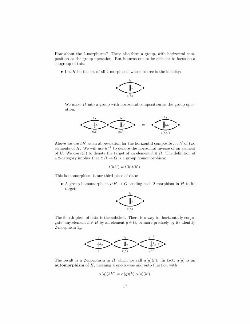
• Let H be the set of all 2-morphisms whose source is the identity:
• •
1•
zz
t(h)
dd h
We make H into a group with horizontal composition as the group oper-ation:
• •
1•
xx
t(h)
ff h •
1•
xx
t(h′)
ff h′
= • •
1•
zz
t(hh′)
dd hh′
Above we use hh′ as an abbreviation for the horizontal composite h h′ of twoelements of H . We will use h−1 to denote the horizontal inverse of an elementof H . We use t(h) to denote the target of an element h ∈ H . The definition ofa 2-category implies that t:H → G is a group homomorphism:
t(hh′) = t(h)t(h′).
This homomorphism is our third piece of data:
• A group homomorphism t:H → G sending each 2-morphism in H to itstarget:
• •
1•
zz
t(h)
dd h
The fourth piece of data is the subtlest. There is a way to ‘horizontally conju-gate’ any element h ∈ H by an element g ∈ G, or more precisely by its identity2-morphism 1g:
• •
g
xx
g
ff 1g •
1•
xx
t(h)
ff h •
g−1
xx
g−1
ff 1g−1
The result is a 2-morphism in H which we call α(g)(h). In fact, α(g) is anautomorphism of H , meaning a one-to-one and onto function with
α(g)(hh′) = α(g)(h) α(g)(h′).
17
Composing two automorphisms gives another automorphism, and this makesthe automorphisms of H into a group, say Aut(H). Even better, α gives agroup homomorphism
α:G → Aut(H).
Concretely, this means that in addition to the above equation, we have
α(gg′) = α(g)α(g′).
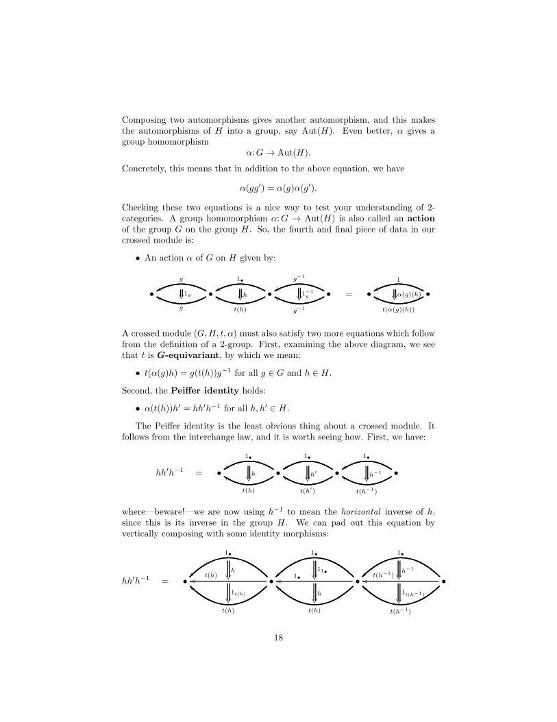
Checking these two equations is a nice way to test your understanding of 2-categories. A group homomorphism α:G → Aut(H) is also called an actionof the group G on the group H . So, the fourth and final piece of data in ourcrossed module is:
• An action α of G on H given by:
• •
g
xx
g
ff 1g •
1•
xx
t(h)
ff h •
g−1
xx
g−1
ff 1−1g = • •
1
xx
t(α(g)(h))
ff α(g)(h)
A crossed module (G,H, t, α) must also satisfy two more equations which followfrom the definition of a 2-group. First, examining the above diagram, we seethat t is G-equivariant, by which we mean:
• t(α(g)h) = g(t(h))g−1 for all g ∈ G and h ∈ H .
Second, the Peiffer identity holds:
• α(t(h))h′ = hh′h−1 for all h, h′ ∈ H .
The Peiffer identity is the least obvious thing about a crossed module. Itfollows from the interchange law, and it is worth seeing how. First, we have:
hh′h−1 = • •
1•
zz
t(h)
dd h
•
1•
zz
t(h′)
dd h′
•
1•
zz
t(h−1)
dd h−1
where—beware!—we are now using h−1 to mean the horizontal inverse of h,since this is its inverse in the group H . We can pad out this equation byvertically composing with some identity morphisms:
hh′h−1 = • •
1•
~~ t(h)oo
t(h)
``
h
1t(h)
•
1•
~~ 1•oo
t(h)
``
11•
h
•
1•
~~ t(h−1)oo
t(h−1)
``
h−1
1t(h−1)
18
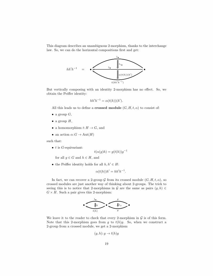
This diagram describes an unambiguous 2-morphism, thanks to the interchangelaw. So, we can do the horizontal compositions first and get:
hh′h−1 = • •
1•
zz 1•oo
t(hh′h−1)
dd
11•
α(t(h))(h′)
But vertically composing with an identity 2-morphism has no effect. So, weobtain the Peiffer identity:
hh′h−1 = α(t(h))(h′).
All this leads us to define a crossed module (G,H, t, α) to consist of:
• a group G,
• a group H ,
• a homomorphism t:H → G, and
• an action α:G → Aut(H)
such that:
• t is G-equivariant:t(α(g)h) = g(t(h))g−1
for all g ∈ G and h ∈ H , and
• the Peiffer identity holds for all h, h′ ∈ H :
α(t(h))h′ = hh′h−1.
In fact, we can recover a 2-group G from its crossed module (G,H, t, α), socrossed modules are just another way of thinking about 2-groups. The trick toseeing this is to notice that 2-morphisms in G are the same as pairs (g, h) ∈G×H . Such a pair gives this 2-morphism:
• •
1•
xx
t(h)
ff h •
g
xx
g
ff 1g
We leave it to the reader to check that every 2-morphism in G is of this form.Note that this 2-morphism goes from g to t(h)g. So, when we construct a2-group from a crossed module, we get a 2-morphism
(g, h): g → t(h)g
19
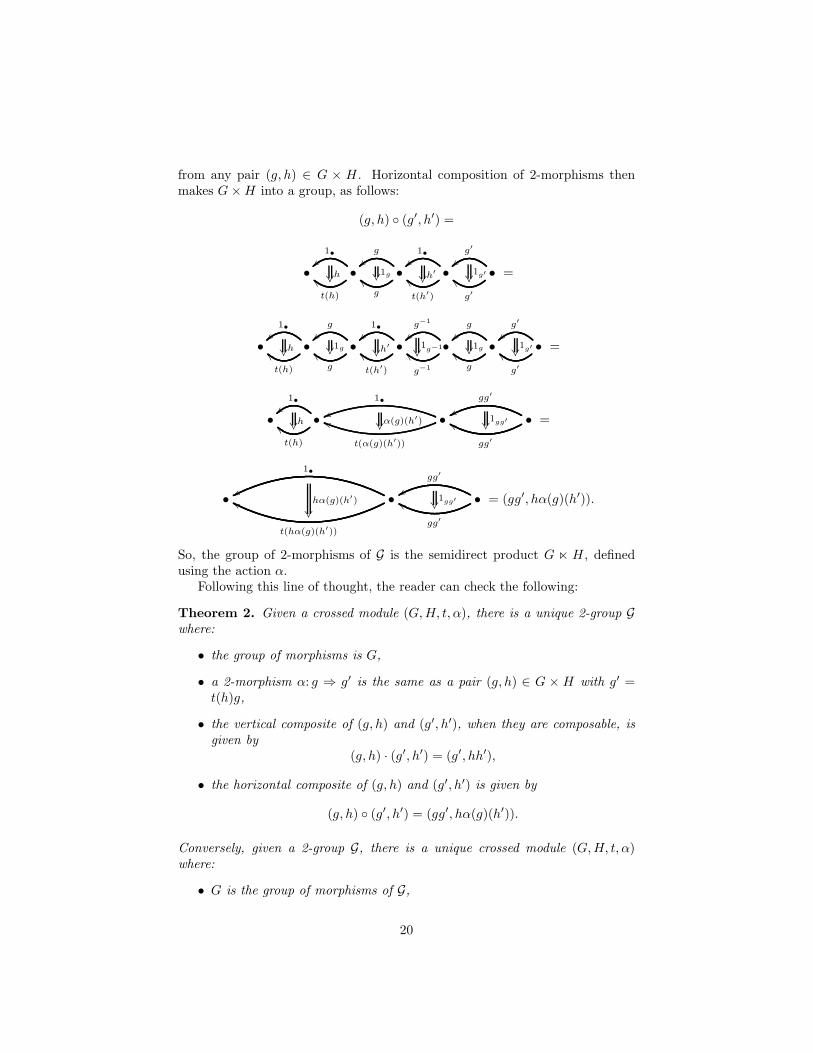
from any pair (g, h) ∈ G × H . Horizontal composition of 2-morphisms thenmakes G×H into a group, as follows:
(g, h) (g′, h′) =
• •
1•
t(h)
aa h •
g
g
aa 1g •
1•
t(h′)
aa h′
•
g′
g′
aa 1g′ =
• •
1•
t(h)
aa h •
g
g
aa 1g •
1•
t(h′)
aa h′
•
g−1
g−1
aa 1g−1 •
g
g
aa 1g •
g′
g′
aa 1g′ =
• •
1•
t(h)
aa h •
1•
uu
t(α(g)(h′))
ii α(g)(h′) •
gg′
xx
gg′
ff 1gg′ =
• •
1•
ww
t(hα(g)(h′))
gg hα(g)(h′)
•
gg′
xx
gg′
ff 1gg′ = (gg′, hα(g)(h′)).
So, the group of 2-morphisms of G is the semidirect product G ⋉ H , definedusing the action α.
Following this line of thought, the reader can check the following:
Theorem 2. Given a crossed module (G,H, t, α), there is a unique 2-group Gwhere:
• the group of morphisms is G,
• a 2-morphism α: g ⇒ g′ is the same as a pair (g, h) ∈ G × H with g′ =t(h)g,
• the vertical composite of (g, h) and (g′, h′), when they are composable, is
given by
(g, h) · (g′, h′) = (g′, hh′),
• the horizontal composite of (g, h) and (g′, h′) is given by
(g, h) (g′, h′) = (gg′, hα(g)(h′)).
Conversely, given a 2-group G, there is a unique crossed module (G,H, t, α)where:
• G is the group of morphisms of G,
20
• H is the group of 2-morphisms with source equal to 1•,
• t:H → G assigns to each 2-morphism in H its target,
• the action α of G on H is given by
α(g)h = 1g h 1g−1 .
Indeed, these two processes set up an equivalence between 2-groups andcrossed modules, as described more formally elsewhere [13, 51]. It thus makessense to define a Lie 2-group to be a 2-group for which the groups G and H inits crossed module are Lie groups, with the maps t:H → G and α:G → Aut(H)being smooth. It is worth emphasizing that in this context we use Aut(H) tomean the group of smooth automorphisms of H . This is a Lie group in its ownright.
In Section 4 we will use Theorem 2 to construct many examples of Lie 2-groups. But first we should finish explaining 2-connections.
3.4 2-Connections
A 2-connection is a recipe for parallel transporting both 0-dimensional and1-dimensional objects—say, particles and strings. Just as we can describe aconnection on a trivial bundle using a Lie-algebra valued differential form, wecan describe a 2-connection using a pair of differential forms. But there is adeeper way of understanding 2-connections. Just as a connection was revealedto be a smooth functor
hol:P1(M) → G
for some Lie group G, a 2-connection will turn out to be a smooth 2-functor
hol:P2(M) → G
for some Lie 2-group G. Of course, to make sense of this we need to define a‘2-functor’, and say what it means for such a thing to be smooth.
The definition of 2-functor is utterly straightforward: it is a map between2-categories that preserves everything in sight. So, given 2-categories C and D,a 2-functor F :C → D consists of:
• a map F sending objects in C to objects in D,
• another map called F sending morphisms in C to morphisms in D,
• a third map called F sending 2-morphisms in C to 2-morphisms in D,
such that:
• given a morphism f :x → y in C, we have F (f):F (x) → F (y),
21
• F preserves composition for morphisms, and identity morphisms:
F (fg) = F (f)F (g)
F (1x) = 1F (x),
• given a 2-morphism α: f ⇒ g in C, we have F (α):F (f) ⇒ F (g),
• F preserves vertical and horizontal composition for 2-morphisms, andidentity 2-morphisms:
F (α · β) = F (α) · F (β)
F (α β) = F (α) F (β)
F (1f ) = 1F (f).
There is a general theory of smooth 2-groupoids and smooth 2-functors [16,88]. But here we prefer to take a more elementary approach. We already knowthat for any Lie 2-group G, the morphisms and 2-morphisms each form Liegroups. Given this, we can say that for any smooth manifold M , a 2-functor
hol:P2(M) → G
is smooth if:
• For any smoothly parametrized family of lazy paths γs (s ∈ [0, 1]n) themorphism hol(γs) depends smoothly on s, and
• For any smoothly parametrized family of lazy surfaces Σs (s ∈ [0, 1]n) the2-morphism hol(Σs) depends smoothly on s.
With these definitions in hand, we are finally ready to understand the basicresult about 2-connections. It is completely analogous to Theorem 1:
Theorem 3. For any Lie 2-group G and any smooth manifold M , there is a
one-to-one correspondence between:
1. 2-connections on the trivial principal G-2-bundle over M ,
2. pairs consisting of a smooth g-valued 1-form A and a smooth h-valued
2-form B on M , such that
t(B) = dA+A ∧A
where we use t: h → g, the differential of the map t:H → G, to convert Binto a g-valued 2-form, and
3. smooth 2-functors
hol:P2(M) → G
where P2(M) is the path 2-groupoid of M .
22
This result was announced by Baez and Schreiber [16], and a proof can bebe found in the work of Schreiber and Waldorf [88]. This work was deeplyinspired by the ideas of Breen and Messing [29, 30], who considered a specialclass of 2-groups, and omitted the equation t(B) = dA+A∧A, since their sortof connection did not assign holonomies to surfaces. One should also comparethe closely related work of Mackaay, Martins, and Picken [67, 69], and the workof Pfeiffer and Girelli [76, 58].
In the above theorem, the first item mentions ‘2-connections’ and ‘2-bundles’—concepts that we have not defined. But since we are only talking about 2-connections on trivial 2-bundles, we do not need these general concepts yet.For now, we can take the third item as the definition of the first. Then the con-tent of the theorem lies in the differential form description of smooth 2-functorshol:P2(M) → G. This is what we need to understand.
A 2-functor of this sort must assign holonomies both to paths and sur-faces. As you might expect, the 1-form A is primarily responsible for defin-ing holonomies along paths, while the 2-form B is responsible for definingholonomies for surfaces. But this is a bit of an oversimplification. When com-puting the holonomy of a surface, we need to use A as well as B!
Another surprising thing is that A and B need to be related by an equation
for the holonomy to be a 2-functor. If we ponder how the holonomy of a surfaceis actually computed, we can see why this is so. We shall not be at all rigoroushere. We just want to give a rough intuitive idea of how to compute a holonomyfor a surface, and where the equation t(B) = dA+A∧A comes from. Of course
dA+A ∧ A = F
is just the curvature of the connection A. This is a big clue.Suppose we are trying to compute the holonomy for a surface starting from
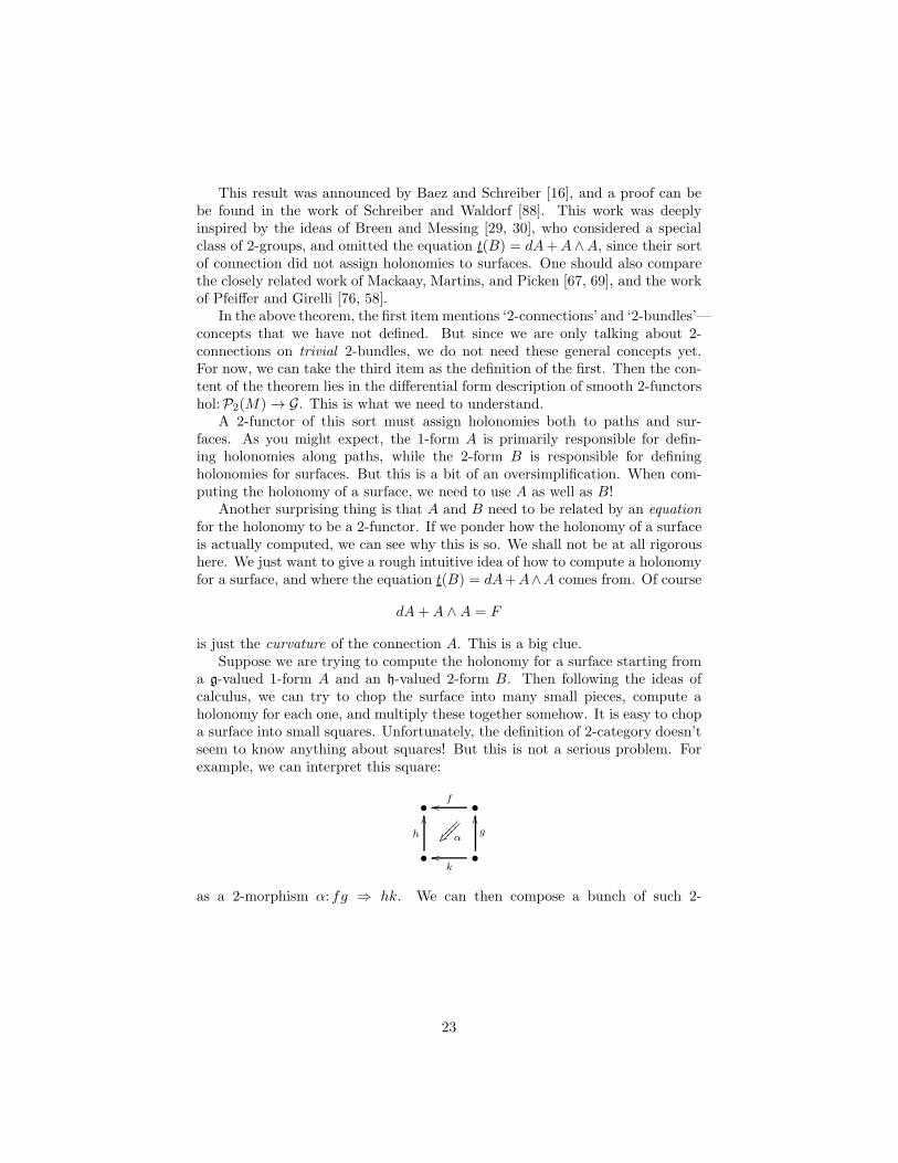
a g-valued 1-form A and an h-valued 2-form B. Then following the ideas ofcalculus, we can try to chop the surface into many small pieces, compute aholonomy for each one, and multiply these together somehow. It is easy to chopa surface into small squares. Unfortunately, the definition of 2-category doesn’tseem to know anything about squares! But this is not a serious problem. Forexample, we can interpret this square:
• •foo
•
h
OO
•k
oo
g
OO
α ⑧⑧⑧⑧⑧⑧⑧⑧
as a 2-morphism α: fg ⇒ hk. We can then compose a bunch of such 2-
23
morphisms:• •oo •oo •oo
•
OO
•oo
OO
•oo
OO
•oo
OO
⑧⑧⑧⑧⑧⑧⑧⑧
⑧⑧⑧⑧⑧⑧⑧⑧
⑧⑧⑧⑧⑧⑧⑧⑧
•
OO
•oo
OO
•oo
OO
•oo
OO
⑧⑧⑧⑧⑧⑧⑧⑧
⑧⑧⑧⑧⑧⑧⑧⑧
⑧⑧⑧⑧⑧⑧⑧⑧
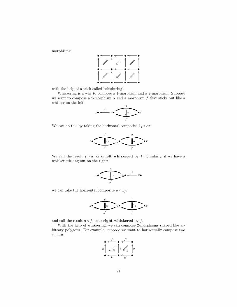
with the help of a trick called ‘whiskering’.Whiskering is a way to compose a 1-morphism and a 2-morphism. Suppose
we want to compose a 2-morphism α and a morphism f that sticks out like awhisker on the left:
z• y•foo •x
g
ww
g′
gg α
We can do this by taking the horizontal composite 1f α:
z• y•
f
vv
f
hh 1f
•x
g
ww
g′
gg α
We call the result f α, or α left whiskered by f . Similarly, if we have awhisker sticking out on the right:
z• y•
g
vv
g′
hh α
x•foo
we can take the horizontal composite α 1f :
z• y•
g
vv
g′
hh α
•x
f
ww
f
gg 1f
and call the result α f , or α right whiskered by f .With the help of whiskering, we can compose 2-morphisms shaped like ar-
bitrary polygons. For example, suppose we want to horizontally compose twosquares:
• •foo •
f ′
oo
•
h
OO
•k
oo
ℓ
OO
•k′
oo
g
OO
α ⑧⑧⑧⑧⑧⑧⑧⑧
β ⑧⑧⑧⑧⑧⑧⑧⑧
24
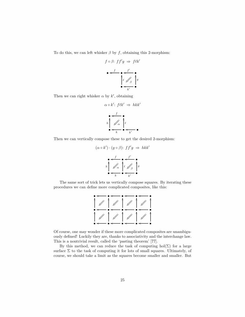
To do this, we can left whisker β by f , obtaining this 2-morphism:
f β: ff ′g ⇒ fℓk′
• •foo •
f ′
oo
•
ℓ
OO
•k′
oo
g
OO
β ⑧⑧⑧⑧⑧⑧⑧⑧
Then we can right whisker α by k′, obtaining
α k′: fℓk′ ⇒ hkk′
• •foo
•
h
OO
•k
oo
ℓ
OO
•k′
ooα ⑧⑧⑧⑧⑧⑧⑧⑧
Then we can vertically compose these to get the desired 2-morphism:
(α k′) · (g β): ff ′g ⇒ hkk′
• •foo •
f ′
oo
•
h
OO
•k
oo
ℓ
OO
•k′
oo
g
OO
α ⑧⑧⑧⑧⑧⑧⑧⑧
β ⑧⑧⑧⑧⑧⑧⑧⑧
The same sort of trick lets us vertically compose squares. By iterating theseprocedures we can define more complicated composites, like this:
• •oo •oo •oo •oo
•
OO
•oo
OO
•oo
OO
•oo
OO
•oo
OO
⑧⑧⑧⑧⑧⑧⑧⑧
⑧⑧⑧⑧⑧⑧⑧⑧
⑧⑧⑧⑧⑧⑧⑧⑧
⑧⑧⑧⑧⑧⑧⑧⑧
•
OO
•oo
OO
•oo
OO
•oo
OO
•oo
OO
⑧⑧⑧⑧⑧⑧⑧⑧
⑧⑧⑧⑧⑧⑧⑧⑧
⑧⑧⑧⑧⑧⑧⑧⑧
⑧⑧⑧⑧⑧⑧⑧⑧
Of course, one may wonder if these more complicated composites are unambigu-ously defined! Luckily they are, thanks to associativity and the interchange law.This is a nontrivial result, called the ‘pasting theorem’ [77].
By this method, we can reduce the task of computing hol(Σ) for a largesurface Σ to the task of computing it for lots of small squares. Ultimately, ofcourse, we should take a limit as the squares become smaller and smaller. But
25
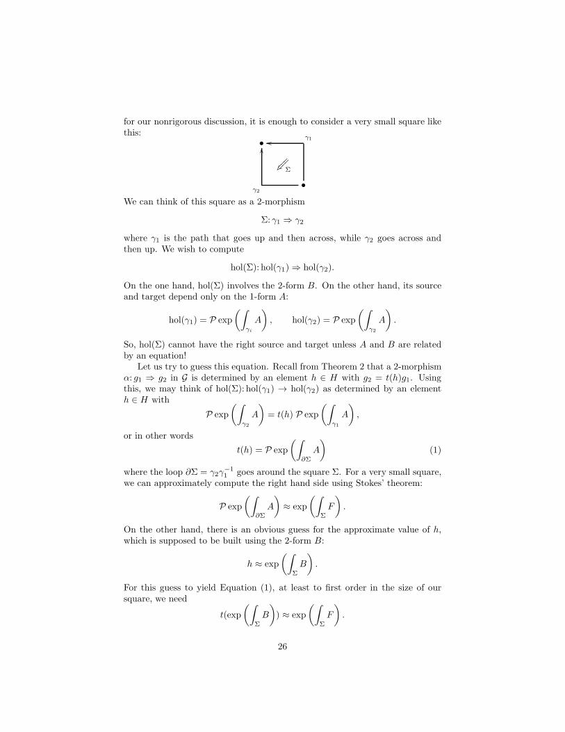
for our nonrigorous discussion, it is enough to consider a very small square likethis:
•
•
Σ ⑧⑧⑧⑧⑧⑧
ooOO
γ2
γ1
We can think of this square as a 2-morphism
Σ: γ1 ⇒ γ2
where γ1 is the path that goes up and then across, while γ2 goes across andthen up. We wish to compute
hol(Σ): hol(γ1) ⇒ hol(γ2).
On the one hand, hol(Σ) involves the 2-form B. On the other hand, its sourceand target depend only on the 1-form A:
hol(γ1) = P exp
(∫
γi
A
)
, hol(γ2) = P exp
(∫
γ2
A
)
.
So, hol(Σ) cannot have the right source and target unless A and B are relatedby an equation!
Let us try to guess this equation. Recall from Theorem 2 that a 2-morphismα: g1 ⇒ g2 in G is determined by an element h ∈ H with g2 = t(h)g1. Usingthis, we may think of hol(Σ): hol(γ1) → hol(γ2) as determined by an elementh ∈ H with
P exp
(∫
γ2
A
)
= t(h) P exp
(∫
γ1
A
)
,
or in other words
t(h) = P exp
(∫
∂Σ
A
)
(1)
where the loop ∂Σ = γ2γ−11 goes around the square Σ. For a very small square,
we can approximately compute the right hand side using Stokes’ theorem:
P exp
(∫
∂Σ
A
)
≈ exp
(∫
Σ
F
)
.
On the other hand, there is an obvious guess for the approximate value of h,which is supposed to be built using the 2-form B:
h ≈ exp
(∫
Σ
B
)
.
For this guess to yield Equation (1), at least to first order in the size of oursquare, we need
t(exp
(∫
Σ
B
)
) ≈ exp
(∫
Σ
F
)
.
26
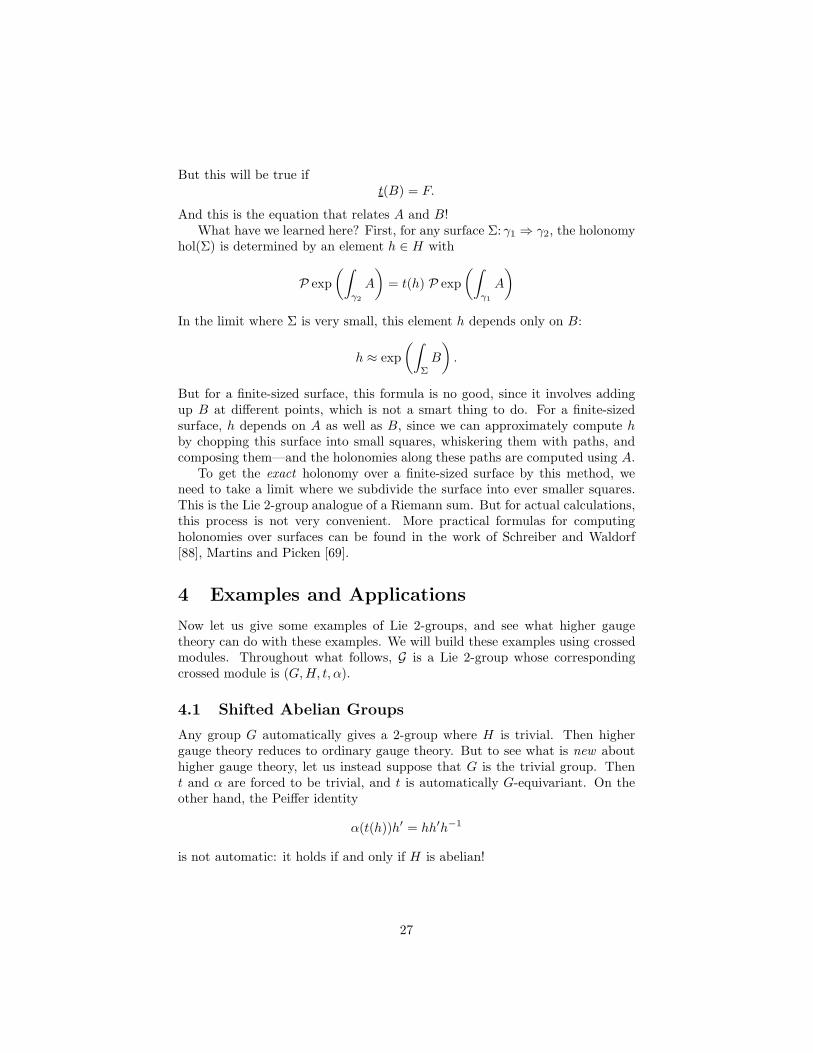
But this will be true ift(B) = F.
And this is the equation that relates A and B!What have we learned here? First, for any surface Σ: γ1 ⇒ γ2, the holonomy
hol(Σ) is determined by an element h ∈ H with
P exp
(∫
γ2
A
)
= t(h) P exp
(∫
γ1
A
)
In the limit where Σ is very small, this element h depends only on B:
h ≈ exp
(∫
Σ
B
)
.
But for a finite-sized surface, this formula is no good, since it involves addingup B at different points, which is not a smart thing to do. For a finite-sizedsurface, h depends on A as well as B, since we can approximately compute hby chopping this surface into small squares, whiskering them with paths, andcomposing them—and the holonomies along these paths are computed using A.
To get the exact holonomy over a finite-sized surface by this method, weneed to take a limit where we subdivide the surface into ever smaller squares.This is the Lie 2-group analogue of a Riemann sum. But for actual calculations,this process is not very convenient. More practical formulas for computingholonomies over surfaces can be found in the work of Schreiber and Waldorf[88], Martins and Picken [69].
4 Examples and Applications
Now let us give some examples of Lie 2-groups, and see what higher gaugetheory can do with these examples. We will build these examples using crossedmodules. Throughout what follows, G is a Lie 2-group whose correspondingcrossed module is (G,H, t, α).
4.1 Shifted Abelian Groups
Any group G automatically gives a 2-group where H is trivial. Then highergauge theory reduces to ordinary gauge theory. But to see what is new abouthigher gauge theory, let us instead suppose that G is the trivial group. Thent and α are forced to be trivial, and t is automatically G-equivariant. On theother hand, the Peiffer identity
α(t(h))h′ = hh′h−1
is not automatic: it holds if and only if H is abelian!
27
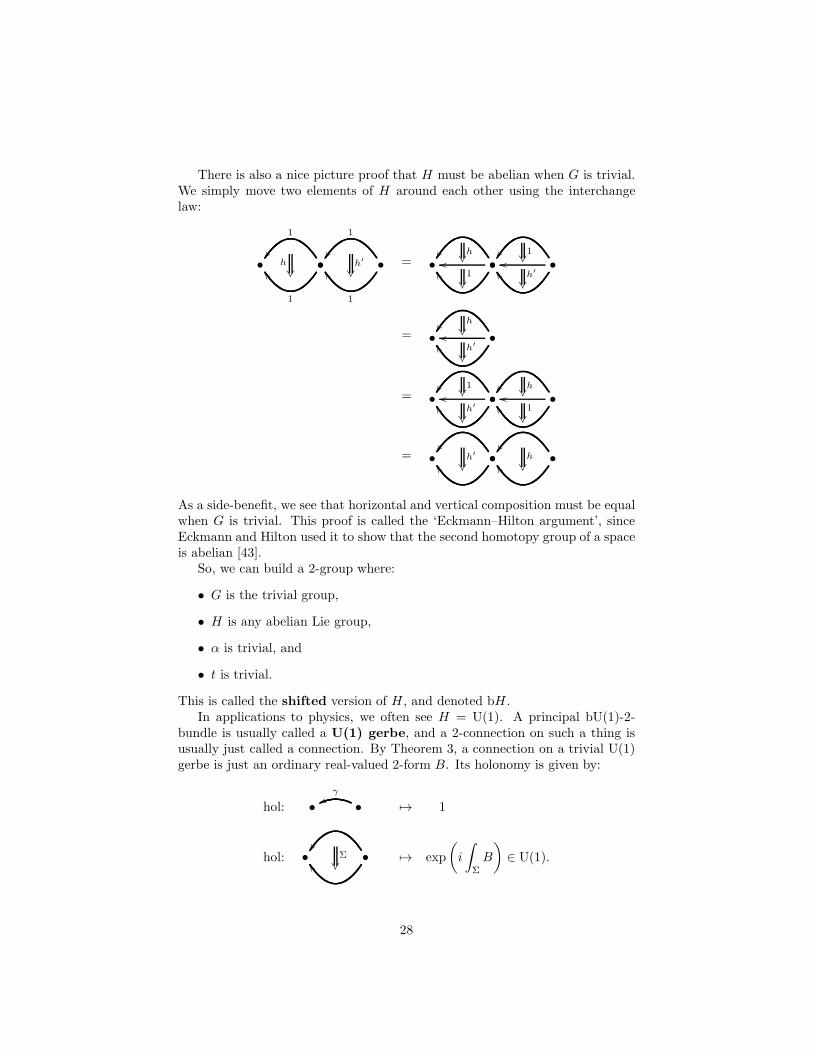
There is also a nice picture proof that H must be abelian when G is trivial.We simply move two elements of H around each other using the interchangelaw:
• •
1
ZZ
1
h
• •
1
ZZ
1
h′
= • •ooYY
h1
• •ooYY 1
h′
= • •YY oo
h
h′
= • •ooYY 1
h′
• •ooYY h
1
= • •ZZ
h′
• •ZZ
h
As a side-benefit, we see that horizontal and vertical composition must be equalwhen G is trivial. This proof is called the ‘Eckmann–Hilton argument’, sinceEckmann and Hilton used it to show that the second homotopy group of a spaceis abelian [43].
So, we can build a 2-group where:
• G is the trivial group,
• H is any abelian Lie group,
• α is trivial, and
• t is trivial.
This is called the shifted version of H , and denoted bH .In applications to physics, we often see H = U(1). A principal bU(1)-2-
bundle is usually called a U(1) gerbe, and a 2-connection on such a thing isusually just called a connection. By Theorem 3, a connection on a trivial U(1)gerbe is just an ordinary real-valued 2-form B. Its holonomy is given by:
hol: • •
γvv
7→ 1
hol: • •ZZ
Σ
7→ exp
(
i
∫
Σ
B
)
∈ U(1).
28
The book by Brylinski [31] gives a rather extensive introduction to U(1)gerbes and their applications. Murray’s theory of ‘bundle gerbes’ gives a dif-ferent viewpoint [74, 89]. Here let us discuss two places where U(1) gerbesshow up in physics. One is ‘multisymplectic geometry’; the other is ‘2-formelectromagnetism’. The two are closely related.
First, let us remember how 1-forms show up in symplectic geometry andelectromagnetism. Suppose we have a point particle moving in some manifoldM . At any time its position is a point q ∈ M and its momentum is a cotangentvector p ∈ T ∗
q M . As time passes, its position and momentum trace out a curve
γ: [0, 1] → T ∗M.
The action of this path is given by
S(γ) =
∫
γ
(
piqi −H(q, p)
)
dt
where H :T ∗M → R is the Hamiltonian. But now suppose the Hamiltonianis zero! Then there is still a nontrivial action, due to the first term. We canrewrite it as follows:
S(γ) =
∫
γ
α
where the 1-formα = pidq
i
is a canonical structure on the cotangent bundle. We can think of α as connec-tion on a trivial U(1)-bundle over T ∗M . Physically, this connection describeshow a quantum particle changes phase even when the Hamiltonian is zero! Thechange in phase is computed by exponentiating the action. So, we have:
hol(γ) = exp
(
i
∫
γ
α
)
.
Next, suppose we carry our particle around a small loop γ which bounds adisk D. Then Stokes’ theorem gives
S(γ) =
∫
γ
α =
∫
D
dα
Here the 2-formω = dα = dpi ∧ dqi
is the curvature of the connection α. It makes T ∗M into a symplectic man-ifold, that is, a manifold with a closed 2-form ω satisfying the nondegeneracycondition
∀v ω(u, v) = 0 =⇒ u = 0.
29
The subject of symplectic geometry is vast and deep, but sometimes this simplepoint is neglected: the symplectic structure describes the change in phase of aquantum particle as we move it around a loop:
hol(γ) = exp
(
i
∫
D
ω
)
.
Perhaps this justifies calling a symplectic manifold a ‘phase space’, though his-torically this seems to be just a coincidence.
It may seem strange to talk about a quantum particle tracing out a loopin phase space, since in quantum mechanics we cannot simultaneously know aparticle’s position and momentum. However, there is a long line of work, begin-ning with Feynman, which computes time evolution by an integral over pathsin phase space [40]. This idea is also implicit in geometric quantization, wherethe first step is to equip the phase space with a principal U(1)-bundle having aconnection whose curvature is the symplectic structure. (Our discussion so faris limited to trivial bundles, but everything we say generalizes to the nontrivialcase.)
Next, consider a charged particle in an electromagnetic field. Suppose thatwe can describe the electromagnetic field using a vector potential A which isa connection on trivial U(1) bundles over M . Then we can pull A back viathe projection π:T ∗M → M , obtaining a 2-form π∗A on phase space. In theabsence of any other Hamiltonian, the particle’s action as we move it along apath γ in phase space will be
S(γ) =
∫
γ
α+ e π∗A
if the particle has charge e. In short, the electromagnetic field changes the
connection on phase space from α to α+ e π∗A. Similarly, when the path γ is aloop bounding a disk D, we have
S(γ) =
∫
D
ω + e π∗F
where F = dA is the electromagnetic field strength. So, electromagnetism alsochanges the symplectic structure on phase space from ω to ω+ e π∗F . For moreon this, see Guillemin and Sternberg [60], who also treat the case of nonabeliangauge fields.
All of this has an analog where particles are replaced by strings. It has beenknown for some time that just as the electromagnetic vector potential naturallycouples to point particles, there is a 2-form B called the Kalb–Ramond fieldwhich naturally couples to strings. The action for this coupling is obtainedsimply by integrating B over the string worldsheet. In 1986, Gawedski [54]showed that the B field should be seen as a connection on a U(1) gerbe. LaterFreed and Witten [52] showed this viewpoint was crucial for understandinganomaly cancellation. However, these authors did not actually use the word
30
‘gerbe’. The role of gerbes was later made explicit by Carey, Johnson andMurray [34], and even more so by Gawedski and Reis [55].
In short, electromagnetism has a ‘higher version’. What about symplecticgeometry? This also has a higher version, which dates back to 1935 work byDeDonder [39] and Weyl [92]. The idea here is that an n-dimensional classicalfield theory has a kind of finite-dimensional phase space equipped with a closed(n+ 2)-form ω which is nondegenerate in the following sense:
∀v1, . . . , vn+1 ω(u, v1, . . . , vn) = 0 =⇒ u = 0.
Such a n-form is called a multisymplectic structure, or more specifically, ann-plectic structure For a nice introduction to multisymplectic geometry, seethe paper by Gotay, Isenberg, Marsden, and Montgomery [57].
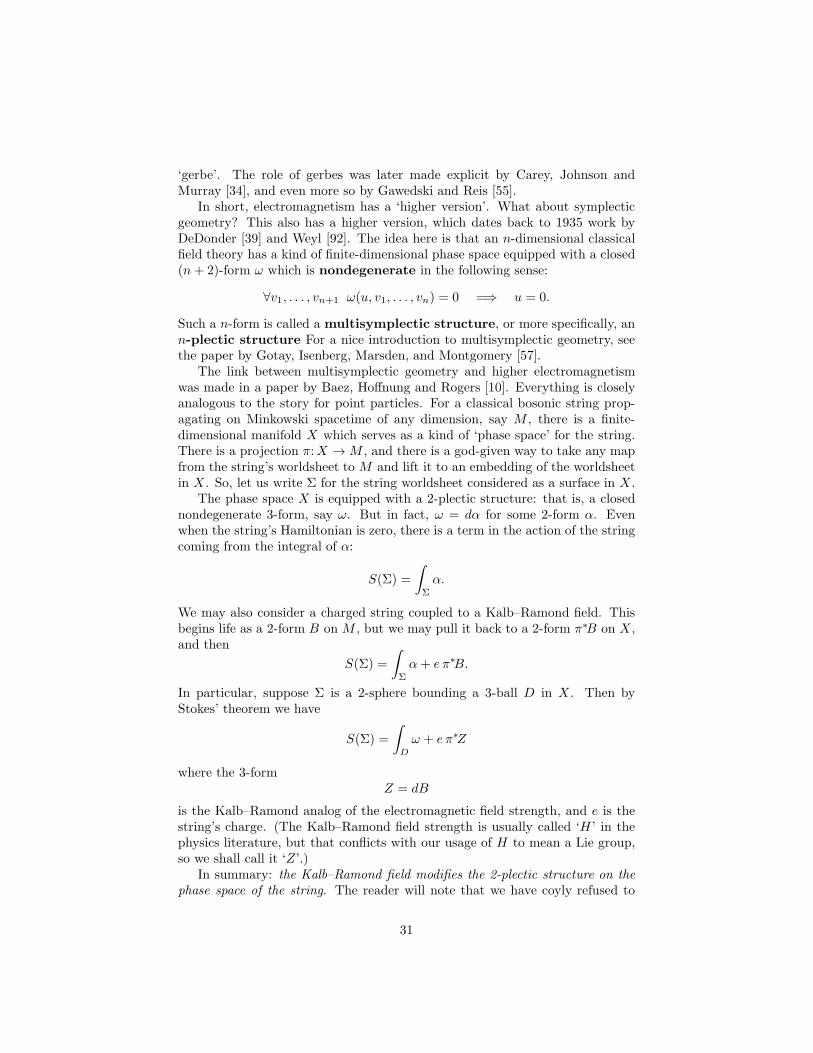
The link between multisymplectic geometry and higher electromagnetismwas made in a paper by Baez, Hoffnung and Rogers [10]. Everything is closelyanalogous to the story for point particles. For a classical bosonic string prop-agating on Minkowski spacetime of any dimension, say M , there is a finite-dimensional manifold X which serves as a kind of ‘phase space’ for the string.There is a projection π:X → M , and there is a god-given way to take any mapfrom the string’s worldsheet to M and lift it to an embedding of the worldsheetin X . So, let us write Σ for the string worldsheet considered as a surface in X .
The phase space X is equipped with a 2-plectic structure: that is, a closednondegenerate 3-form, say ω. But in fact, ω = dα for some 2-form α. Evenwhen the string’s Hamiltonian is zero, there is a term in the action of the stringcoming from the integral of α:
S(Σ) =
∫
Σ
α.
We may also consider a charged string coupled to a Kalb–Ramond field. Thisbegins life as a 2-form B on M , but we may pull it back to a 2-form π∗B on X ,and then
S(Σ) =
∫
Σ
α+ e π∗B.
In particular, suppose Σ is a 2-sphere bounding a 3-ball D in X . Then byStokes’ theorem we have
S(Σ) =
∫
D
ω + e π∗Z
where the 3-formZ = dB
is the Kalb–Ramond analog of the electromagnetic field strength, and e is thestring’s charge. (The Kalb–Ramond field strength is usually called ‘H ’ in thephysics literature, but that conflicts with our usage of H to mean a Lie group,so we shall call it ‘Z’.)
In summary: the Kalb–Ramond field modifies the 2-plectic structure on the
phase space of the string. The reader will note that we have coyly refused to
31
describe the phase space X or its 2-form α. For this, see the paper by Baez,Hoffnung and Rogers [10]. In this paper, we explain how the usual dynamics of aclassical bosonic string coupled to a Kalb–Ramond field can be described usingmultisymplectic geometry. We also explain how to generalize Poisson bracketsfrom symplectic geometry to multisymplectic geometry. Just as Poisson bracketsin symplectic geometry make the functions on phase space into a Lie algebra,Poisson brackets in multisymplectic geometry give rise to a ‘Lie 2-algebra’. Lie2-algebras are also important in higher gauge theory in the same way that Liealgebras are important for gauge theory. Indeed, the ‘string 2-group’ describedin Section 4.6 was constructed only after its Lie 2-algebra was found [7]. Later,this Lie 2-algebra was seen to arise naturally from multisymplectic geometry[15].
4.2 The Poincare 2-Group
Suppose we have a representation α of a Lie group G on a finite-dimensionalvector space H . We can regard H as an abelian Lie group with addition as thegroup operation. This lets us regard α as an action of G on this abelian Liegroup. So, we can build a 2-group G where:
• G is any Lie group,
• H is any vector space,
• α is the representation of G on H , and
• t is trivial.
In particular, note that the Peiffer identity holds. In this way, we see thatany group representation gives a crossed module—so group representations aresecretly 2-groups!
For example, if we let G be the Lorentz group and let α be its obviousrepresentation on R4:
G = SO(3, 1)
H = R4
we obtain the so-called Poincare 2-group, which has the Lorentz group as itsgroup of morphisms, and the Poincare group as its group of 2-morphisms [13].
What is the Poincare 2-group good for? It is not clear, but there are someclues. Just as we can study representations of groups on vector spaces, we canstudy representations of 2-groups on ‘2-vector spaces’ [6, 24, 38, 48]. The rep-resentations of a group are the objects of a category, and this sort of categorycan be used to build ‘spin foam models’ of background-free quantum field theo-ries [5]. This endeavor has been most successful with 3d quantum gravity [53],but everyone working on this subject dreams of doing something similar for 4dquantum gravity [80]. Going from groups to 2-groups boosts the dimension ofeverything: the representations of a 2-group are the objects of a 2-category, andCrane and Sheppeard outlined a program for building a 4-dimensional spin foam
32
model starting from the 2-category of representations of the Poincare 2-group[36].
Crane and Sheppeard hoped their model would be related to quantum grav-ity in 4 spacetime dimensions. This has not come to pass, at least not yet—butthis spin foam model does have interesting connections to 4d physics. The spinfoam model of 3d quantum gravity automatically includes point particles, andBaratin and Freidel have shown that it reduces to the usual theory of Feynmandiagrams in 3d Minkowski spacetime in the limit where the gravitational con-stant GNewton goes to zero [21]. This line of thought led Baratin and Freidel toconstruct a spin foam model that is equivalent to the usual theory of Feynmandiagrams in 4d Minkowski spacetime [22]. At first the mathematics underlyingthis model was a bit mysterious—but it now seems clear that this model is basedon the representation theory of the Poincare 2-group! For a preliminary reporton this fascinating research, see the paper by Baratin and Wise [23].
In short, it appears that the 2-category of representations of the Poincare2-group gives a spin foam description of quantum field theory on 4d Minkowskispacetime. Unfortunately, while spin foam models in 3 dimensions can be ob-tained by quantizing gauge theories, we do not see how to obtain this 4d spinfoam model by quantizing a higher gauge theory. Indeed, we know of no classi-cal field theory in 4 dimensions whose solutions are 2-connections on a principalG-2-bundle where G is the Poincare 2-group.
However, if we replace the Poincare 2-group by a closely related 2-group,this puzzle does have a nice solution. Namely, if we take
G = SO(3, 1)
H = so(3, 1)
and take α to be the adjoint representation, we obtain the ‘tangent 2-group’ ofthe Lorentz group. As we shall see, 2-connections for this 2-group arise naturallyas solutions of a 4d field theory called ‘topological gravity’.
4.3 Tangent 2-Groups
We have seen that any group representation gives a 2-group. But any Lie groupG has a representation on its own Lie algebra: the adjoint representation. Thislets us build a 2-group from the crossed module where:
• G is any Lie group,
• H is g regarded as a vector space and thus an abelian Lie group,
• α is the adjoint representation, and
• t is trivial.
We call this the tangent 2-group T G of the Lie group G. Why? We havealready seen that for any Lie 2-group, the group of all 2-morphisms is thesemidirect product G⋉H . In the case at hand, this semidirect product is just
33
G ⋉ g, with G acting on g via the adjoint representation. But as a manifold,this semidirect product is nothing other than the tangent bundle TG of the Liegroup G. So, the tangent bundle TG becomes a group, and this is the group of2-morphisms of T G.
By Theorem 3, a 2-connection on a trivial T G-2-bundle consists of a g-valued1-form A and a g-valued 2-form B such that the curvature F = dA + A ∧ Asatisfies
F = 0,
since t(B) = 0 in this case. Where can we find such 2-connections? We can findthem as solutions of a field theory called 4-dimensional BF theory!
BF theory is a classical field theory that works in any dimension. So, take ann-dimensional oriented manifold M as our spacetime. The fields in BF theoryare a connection A on the trivial principal G-bundle over M , together with ag-valued (n− 2)-form B. The action is given by
S(A,B) =
∫
M
tr(B ∧ F ).
Setting the variation of this action equal to zero, we obtain the following fieldequations:
dB + [A,B] = 0, F = 0.
In dimension 4, B is a g-valued 2-form—and thanks to the second equation, Aand B fit together to define a 2-connection on the trivial T G-2-bundle over M .
It may seem dull to study a gauge theory where the equations of motionimply the connection is flat. But there is still room for some fun. We see thisalready in 3-dimensional BF theory, where B is a g-valued 1-form rather than a2-form. This lets us package A and B into a connection on the trivial TG-bundleover M . The field equations
dB + [A,B] = 0, F = 0
then say precisely that this connection is flat.When the group G is the Lorentz group SO(2, 1), TG is the corresponding
Poincare group. With this choice of G, 3d BF theory is a version of 3d generalrelativity. In 3 dimensions, unlike the more physical 4d case, the equationsof general relativity say that spacetime is flat in the absence of matter. Andat first glance, 3d BF theory only describes general relativity without matter.After all, its solutions are flat connections.
Nonetheless, we can consider 3d BF theory on a manifold from which theworldline of a point particle has been removed. In the Bohm–Aharonov effect, ifwe carry a charged object around a solenoid, we obtain a nontrivial phase eventhough the U(1) connection A is flat outside the solenoid. Similarly, in 3d BFtheory, the connection (A,B) will be flat away from the particle’s worldline, but
34
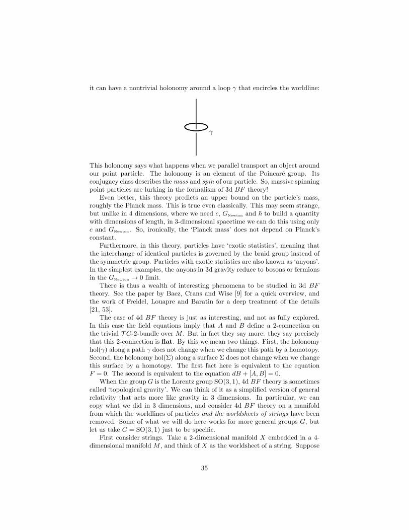
it can have a nontrivial holonomy around a loop γ that encircles the worldline:
γ
This holonomy says what happens when we parallel transport an object aroundour point particle. The holonomy is an element of the Poincare group. Itsconjugacy class describes themass and spin of our particle. So, massive spinningpoint particles are lurking in the formalism of 3d BF theory!
Even better, this theory predicts an upper bound on the particle’s mass,roughly the Planck mass. This is true even classically. This may seem strange,but unlike in 4 dimensions, where we need c, GNewton and ~ to build a quantitywith dimensions of length, in 3-dimensional spacetime we can do this using onlyc and GNewton. So, ironically, the ‘Planck mass’ does not depend on Planck’sconstant.
Furthermore, in this theory, particles have ‘exotic statistics’, meaning thatthe interchange of identical particles is governed by the braid group instead ofthe symmetric group. Particles with exotic statistics are also known as ‘anyons’.In the simplest examples, the anyons in 3d gravity reduce to bosons or fermionsin the GNewton → 0 limit.
There is thus a wealth of interesting phenomena to be studied in 3d BFtheory. See the paper by Baez, Crans and Wise [9] for a quick overview, andthe work of Freidel, Louapre and Baratin for a deep treatment of the details[21, 53].
The case of 4d BF theory is just as interesting, and not as fully explored.In this case the field equations imply that A and B define a 2-connection onthe trivial T G-2-bundle over M . But in fact they say more: they say preciselythat this 2-connection is flat. By this we mean two things. First, the holonomyhol(γ) along a path γ does not change when we change this path by a homotopy.Second, the holonomy hol(Σ) along a surface Σ does not change when we changethis surface by a homotopy. The first fact here is equivalent to the equationF = 0. The second is equivalent to the equation dB + [A,B] = 0.
When the group G is the Lorentz group SO(3, 1), 4d BF theory is sometimescalled ‘topological gravity’. We can think of it as a simplified version of generalrelativity that acts more like gravity in 3 dimensions. In particular, we cancopy what we did in 3 dimensions, and consider 4d BF theory on a manifoldfrom which the worldlines of particles and the worldsheets of strings have beenremoved. Some of what we will do here works for more general groups G, butlet us take G = SO(3, 1) just to be specific.
First consider strings. Take a 2-dimensional manifold X embedded in a 4-dimensional manifold M , and think of X as the worldsheet of a string. Suppose
35
we can find a small loop γ that encircles X in such a way that γ is contractiblein M but not in M −X . If we do 4d BF theory on the spacetime M −X , theholonomy
hol(γ) ∈ SO(3, 1)
will not change when we apply a homotopy to γ. This holonomy describes the‘mass density’ of our string [9, 20].
Next, consider particles. Take a curve C embedded in M , and think of C asthe worldline of a particle. Suppose we can find a small 2-sphere Σ in M − Cthat is contractible in M but not M − C. We can think of this 2-sphere as a2-morphism Σ: 1x ⇒ 1x in the path 2-groupoid of M . If we do 4d BF theoryon the spacetime M − C, the holonomy
hol(Σ) ∈ so(3, 1)
will not change when we apply a homotopy to Σ. So, this holonomy describessome information about the particle—but so far as we know, the physical mean-ing of this information has not been worked out.
What if we had a field theory whose solutions were flat 2-connections for thePoincare 2-group? Then we would have
hol(Σ) ∈ R4
and there would be a tempting interpretation of this quantity: namely, as theenergy-momentum of our point particle. So, the puzzle posed at the end of theprevious section is a tantalizing one.
One may rightly ask if the ‘strings’ described above bear any relation to thoseof string theory. If they are merely surfaces cut out of spacetime, they lack thedynamical degrees of freedom normally associated to a string. Certainly theydo not have an action proportional to their surface area, as for the Polyakovstring. Indeed, one may ask if ‘area’ even makes sense in 4d BF theory. Afterall, there is no metric on spacetime: the closest substitute is the so(3, 1)-valued2-form B.
Some of these problems may have solutions. For starters, when we removea surface X from our 4-manifold M , the action
S(A,B) =
∫
M−X
tr(B ∧ F )
is no longer gauge-invariant: a gauge transformation changes the action by aboundary term which is an integral over X . We can remedy this by introducingfields that live on X , and adding a term to the action which is an integral overXinvolving these fields. There are a number of ways to do this [14, 49, 59, 50, 73].For some, the integral overX is proportional to the area of the string worldsheetin the special case where the B field arises from a cotetrad (that is, an R4-valued1-form) as follows:
B = e ∧ e
36
where we use the isomorphism Λ2R4 ∼= so(3, 1). In this case there is close rela-tion to the Nambu–Goto string, which has been carefully examined by Fairbairn,Noui and Sardelli [50].
This is especially intriguing because when B takes the above form, the BFaction becomes the usual Palatini action for general relativity:
S(A, e) =
∫
M
tr(e ∧ e ∧ F )
where ‘tr’ is a suitable nondegenerate bilinear form on so(3, 1). Unfortunately,solutions of Palatini gravity typically fail to obey the condition t(B) = F whenwe take B = e∧e. So, we cannot construct 2-connections in the sense of Theorem3 from these solutions! If we want to treat general relativity in 4 dimensions asa higher gauge theory, we need other ideas. We describe two possibilities at theend of Section 4.5.
4.4 Inner Automorphism 2-Groups
There is also a Lie 2-group where:
• G is any Lie group,
• H = G,
• t is the identity map,
• α is conjugation:α(g)h = ghg−1.
Following Roberts and Schreiber [79] we call this the inner automorphism2-group of G, and denote it by INN (G). We explain this terminology in thenext section.
A 2-connection on the trivial INN (G)-2-bundle over a manifold consists ofa g-valued 1-form A and a g-valued 2-form B such that
B = F
since t is now the identity. Intriguingly, 2-connections of this sort show up assolutions of a slight variant of 4d BF theory. In a move that he later called hisbiggest blunder, Einstein took general relativity and threw an extra term intothe equations: a ‘cosmological constant’ term, which gives the vacuum nonzeroenergy. We can do the same for topological gravity, or indeed 4d BF theory forany group G. After all, what counts as a blunder for Einstein might count as agood idea for lesser mortals such as ourselves.
So, fix a 4-dimensional oriented manifoldM as our spacetime. As in ordinaryBF theory, take the fields to be a connection A on the trivial principal G-bundleover M , together with a g-valued 2-form B. The action for BF theory ‘withcosmological constant’ is defined to be
S(A,B) =
∫
M
tr(B ∧ F −λ
2B ∧B).
37
Setting the variation of the action equal to zero, we obtain these field equations:
dB + [A,B] = 0, F = λB.
When λ = 0, these are just the equations we saw in the previous section. Butlet us consider the case λ 6= 0. Then these equations have a drastically differentcharacter! The Bianchi identity dF + [A,F ] = 0, together with F = λB,automatically implies that dB + [A,B] = 0. So, to get a solution of this theorywe simply take any connection A, compute its curvature F and set B = F/λ.
This may seem boring: a field theory where any connection is a solution.But in fact it has an interesting relation to higher gauge theory. To see this,it helps to change variables and work with the field β = λB. Then the fieldequations become
dβ + [A, β] = 0, F = β.
Any solution of these equations gives a 2-connection on the trivial principalINN (G)-2-bundle over M !
There is also a tantalizing relation to the cosmological constant in generalrelativity. If the B field arises from a cotetrad as explained in the previoussection:
B = e ∧ e,
then the above action becomes
S =
∫
M
tr(e ∧ e ∧ F −λ
2e ∧ e ∧ e ∧ e).
When we choose the bilinear form ‘tr’ correctly, this is the action for generalrelativity with a cosmological constant proportional to λ.
There is some evidence [4] that BF theory with nonzero cosmological con-stant can be quantized to obtain the so-called Crane–Yetter model [35, 37],which is a spin foam model based on the category of representations of thequantum group associated to G. Indeed, in some circles this is taken almostas an article of faith. But a rigorous argument, or even a fully convincingargument, seems to be missing. So, this issue deserves more study.
The λ → 0 limit of BF theory is fascinating but highly singular, since forλ 6= 0 a solution is just a connection A, while for λ = 0 a solution is a flatconnection A together with a B field such that dB + [A,B] = 0. At leastin some rough intuitive sense, as λ → 0 the group H in the crossed modulecorresponding to INN (G) ‘expands and flattens out’ from the group G to itstangent space g. Thus, INN (G) degenerates to the tangent 2-group T G. Itwould be nice to make this precise using a 2-group version of the theory of groupcontractions.
4.5 Automorphism 2-Groups
The inner automorphism group of the previous section is closely related to theautomorphism 2-group AUT (H), defined using the crossed module where:
38
• G = Aut(H),
• H is any Lie group,
• t:H → Aut(H) sends any group element to the operation of conjugatingby that element,
• α: Aut(H) → Aut(H) is the identity.
We use the term ‘automorphism 2-group’ because AUT (H) really is the 2-groupof symmetries of H . Lie groups form a 2-category, any object in a 2-categoryhas a 2-group of symmetries, and the 2-group of symmetries of H is naturallya Lie 2-group, which is none other than AUT (H). See [13] for details.
A principal AUT (H)-2-bundle is usually called a nonabelian gerbe [28].Nonabelian gerbes are a major test case for ideas in higher gauge theory. Indeed,almost the whole formalism of 2-connections was worked out first for nonabeliangerbes by Breen and Messing [30]. The one aspect they did not consider is theone we have focused on here: parallel transport. Thus, they did not impose theequation t(B) = F , which we need to obtain holonomies satisfying the conditionsof Theorem 3. Nonetheless, the quantity F − t(B) plays an important role inBreen and Messing’s formalism: they call it the fake curvature. Generalizingtheir ideas slightly, for any Lie 2-group G, we may define a connection on atrivial principal G-2-bundle to be a pair consisting of a g-valued 1-form A andan h-valued 2-form. A 2-connection is then a connection with vanishing fakecurvature.
The relation between the automorphism 2-group and the inner automor-phism 2-group is nicely explained in the work of Roberts and Schreiber [79]. Asthey discuss, for any group G there is an exact sequence of 2-groups
1 → Z(G) → INN (G) → AUT (G) → OUT (G) → 1
where Z(G) is the center of G and OUT (G) is the group of outer automorphismsof G, both regarded as 2-groups with only identity 2-morphisms.
Roberts and Schreiber go on to consider an analogous sequence of 3-groupsconstructed starting from a 2-group. Among these, the ‘inner automorphism3-group’ INN (G) of a 2-group G plays a special role [86]. The reason is thatany connection on a principal G-2-bundle, not necessarily obeying t(B) = F ,gives a flat 3-connection on a principal INN (G)-3-bundle! This in turn allowsus to define a version of parallel transport for particles, strings and 2-branes.
This may give a way to understand general relativity in terms of higher gaugetheory. As we have already seen in Section 4.3, Palatini gravity in 4d spacetimeinvolves an so(3, 1)-valued 1-form A and an so(3, 1)-valued 2-form B = e ∧ e.This is precisely the data we expect for a connection on a principal G-2-bundlewhere G is the tangent 2-group of the Lorentz group. Typically this connectionfails to obey the equation t(B) = F . So, it is not a 2-connection. But, it gives aflat 3-connection on an INN (T SO(3, 1))-3-bundle. So, we may optimisticallycall INN (T SO(3, 1)) the gravity 3-group.
39
Does the gravity 3-group actually shed any light on general relativity? Thework of Martins and Picken [70] establishes a useful framework for studyingthese issues. They define a path 3-groupoid P3(M) for a smooth manifold M .Given a Lie 3-group G, they describe 3-connections on the trivial G-3-bundleover M as 3-functors
hol:P3(M) → G
Moreover, they show how to construct these functors from a 1-form, a 2-form,and a 3-form taking values in three Lie algebras associated to G. In the casewhere G = INN (T SO(3, 1)) and hol is a flat 3-connection, this data reducesto an so(3, 1)-valued 1-form A and an so(3, 1)-valued 2-form B.
4.6 String 2-Groups
The Lie 2-groups discussed so far are easy to construct. The string 2-group isconsiderably more subtle. Ultimately it forces upon us a deeper conception ofwhat a Lie 2-group really is, and a more sophisticated approach to higher gaugetheory. Treated in proper detail, these topics would carry us far beyond thelimits of this quick introduction. But it would be a shame not to mention themat all.
Suppose we have a central extension of a Lie group G by an abelian Liegroup A. In other words, suppose we have a short exact sequence of Lie groups
1 → A → Ht→ G → 1
where the image of A lies in the center of H . Then we can construct an actionα of G on H as follows. The map t:H → G describes H as a fiber bundleover G, so choose a section of this bundle: that is, a function s:G → H witht(s(g)) = g, not necessarily a homomorphism. Then set
α(g)h = s(g)hs(g)−1.
Since A is included in the center of H , α is independent of the choice of s.Thanks to this, we do not need a global smooth section s to check that α(g)depends smoothly on g: it suffices that there exist a local smooth section ina neighborhood of each g ∈ G, and indeed this is always true. We can usethese local sections to define α globally, since they must give the same α onoverlapping neighborhoods.
Given all this, we can check that t is G-equivariant and that the Peifferidentity holds. So, we obtain a Lie 2-group where:
• G is any Lie group,
• H is any Lie group,
• t:H → G makes H into a central extension of G,
• α is given by α(g)h = s(g)hs(g)−1 where s:G → H is any section.
40
We call this the central extension 2-group C(Ht→ G).
To get concrete examples, we need examples of central extensions. For anychoice of G and A, we can always take H = G×A and use the ‘trivial’ centralextension
1 → A → A×G → G → 1.
For more interesting examples, we need nontrivial central extensions. Thesetend to arise from problems in quantization. For example, suppose V is a finite-dimensional symplectic vector space: that is, a vector space equipped witha nondegenerate antisymmetric bilinear form
ω:V × V → R.
Then we can make H = V ×R into a Lie group called the Heisenberg group,with the product
(u, a)(v, b) = (u+ v, a+ b+ ω(u, v)).
The Heisenberg group plays a fundamental role in quantum mechanics, becausewe can think of V as the phase space of a classical point particle. If we letG stand for V regarded as an abelian Lie group, then elements of G describetranslations in phase space: that is, translations of both position and momen-tum. The Heisenberg group H describes how these translations commute only‘up to a phase’ when we take quantum mechanics into account: the phase isgiven by exp(iω(u, v)). There is a homomorphism t:H → G that forgets thisphase information, given by
t(u, a) = u.
This exhibits H as a central extension of G. We thus obtain a central extension2-group C(H
t−→G), called the Heisenberg 2-group of the symplectic vector
space V .The applications of Heisenberg 2-groups seem largely unexplored, and should
be worth studying. So far, much more work has been put into understanding 2-groups arising from central extensions of loop groups. The reason is that centralextensions of loop groups play a basic role in string theory and conformal fieldtheory, as nicely explained by Pressley and Segal [78].
Suppose that G is a connected and simply-connected compact simple LiegroupG. Define the loop group ΩG to be the set of all smooth paths γ: [0, 1] →G that start and end at the identity of G. This becomes a group under pointwisemultiplication, and in fact it is a kind of infinite-dimensional Lie group [71].
For each integer k, called the level, the loop group has a central extension
1 → U(1) → ΩkGt
−→ΩG → 1.
These extensions are all different, and all nontrivial except for k = 0. In physics,they arise because the 2d gauge theory called the Wess–Zumino–Witten modelhas an ‘anomaly’. The loop group ΩG acts as gauge transformations in theclassical version of this theory. However, when we quantize the theory, we obtain
41
a representation of ΩG only ‘up to a phase’—that is, a projective representation.This can be understood as an honest representation of the central extension
ΩkG, where the integer k appears in the Lagrangian for the Wess–Zumino–Witten model.
Starting from this central extension we can construct a central extension2-group called the level-k loop 2-group of G, Lk(G). This is an infinite-dimensional Lie 2-group, meaning that it comes from a crossed module wherethe groups involved are infinite-dimensional Lie groups, and all the maps aresmooth. Moreover, it fits into an exact sequence
1 → Lk(G) → ST RINGk(G)−→G → 1
where the middle term, the level-k string 2-group of G, has very interestingproperties [8].
Since the string 2-group ST RINGk(G) is an infinite-dimensional Lie 2-group, it is a topological 2-group. There is a way to take any topological 2-group and squash it down to a topological group [8, 18]. Applying this trickto ST RINGk(G) when k = 1, we obtain a topological group whose homotopygroups match those of G—except for the third homotopy group, which has beenmade trivial. In the special case where G = Spin(n), this topological group iscalled the ‘string group’, since to consistently define superstrings propagatingon a spin manifold, we must reduce its structure group from Spin(n) to thisgroup [94]. The string group also plays a role in Stolz and Teichner’s work onelliptic cohomology, which involves a notion of parallel transport over surfaces[90]. There is a lot of sophisticated mathematics involved here, but ultimatelymuch of it should arise from the way string 2-groups are involved in the paralleltransport of strings! The work of Sati, Schreiber and Stasheff [83] provides goodevidence for this, as does the work of Waldorf [91].
In fact, the string Lie 2-group had lived through many previous incarnationsbefore being constructed as an infinite-dimensional Lie 2-group. Brylinski andMcLaughlin [33] thought of it as a U(1) gerbe over the group G. The fact thatthis gerbe is ‘multiplicative’ makes it something like a group in its own right[32]. This viewpoint has also been explored by Murray and Stevenson [75].
Later, Baez and Crans [7] constructed a Lie 2-algebra stringk(g) correspond-ing to the string Lie 2-group. For pedagogical purposes, our discussion of Lie2-groups has focused solely on ‘strict’ 2-groups, where the 1-morphisms satisfythe group axioms strictly, as equations. However, there is also an extensivetheory of ‘weak’ 2-groups, where the 1-morphisms obey the group axioms onlyup to invertible 2-morphisms [13]. Following this line of thought, we may alsodefine weak Lie 2-algebras [81], and the Lie 2-algebra stringk(g) is one of thesewhere only the Jacobi identity fails to hold strictly.
The beauty of weak Lie 2-algebras is that stringk(g) is very easy to describe inthese terms. In particular, it is finite-dimensional. The hard part is constructinga weak Lie 2-group corresponding to this weak Lie 2-algebra. It is easy to checkthat any strict Lie 2-algebra has a corresponding strict Lie 2-group. Weak Lie 2-algebras are more tricky [13]. Baez, Crans, Schreiber and Stevenson [8] dodged
42
this problem by showing that the string Lie 2-algebra is equivalent (in someprecise sense) to a strict Lie 2-algebra, which however is infinite-dimensional.They then constructed the infinite-dimensional strict Lie 2-group correspondingto this strict Lie 2-algebra. This is just ST RINGk(G) as described above.
On the other hand, a finite-dimensional model of the string 2-group wasrecently introduced by Schommer-Pries [85]. This uses an improved definitionof ‘weak Lie 2-group’, based on an important realization: the correct mapsbetween smooth groupoids are not the smooth functors, but something moregeneral [64]. We have already mentioned this in our discussion of connection:a smooth functor hol:P1(M) → G is a connection on the trivial principal G-bundle over M , while one of these more general maps is a connection on anarbitrary principal G-bundle over M . If we take this lesson to heart, we are ledinto the world of ‘stacks’—and in that world, we can find a finite-dimensionalversion of the string 2-group.
There has also been progress on constructing weak Lie n-groups from weakLie n-algebras for n > 2. Getzler [56] and Henriques [61] have developed anapproach that works for all n, even n = ∞. Their approach is able to handleweak Lie ∞-algebras of a sort known as ‘L∞-algebras’. Quite roughly, theidea is that in an L∞-algebra, the Jacobi identity holds only weakly, while theantisymmetry of the bracket still holds strictly.
In fact, L∞-algebras were developed by Stasheff and collaborators [68, 84]before higher gauge theory became recognized as a subject of study. But morerecently, Sati, Schreiber, Stasheff [82, 83] have developed a lot of higher gaugetheory with the help of L∞-algebras. Thanks to their work, it is becomingclear that superstring theory, supergravity and even the mysterious ‘M -theory’have strong ties to higher gauge theory. For example, they argue that 11-dimensional supergravity can be seen as a higher gauge theory governed by acertain ‘Lie 3-superalgebra’ which they call sugra(10, 1). The number 3 hererelates to the 2-brane solutions of 11-dimensional supergravity: just as paralleltransport of strings is described by 2-connections, the parallel transport of 2-branes is described by 3-connections, which in the supersymmetric case involveLie 3-superalgebras.
In fact, sugra(10, 1) is one of a family of four Lie 3-superalgebras that extendthe Poincare Lie superalgebra in dimensions 4, 5, 7 and 11. These can be builtvia a systematic construction starting from the four normed division algebras:the real numbers, the complex numbers, the quaternions and the octonions [11].These four algebras also give rise to Lie 2-superalgebras extending the PoincareLie superalgebra in dimensions 3, 4, 6, and 10. The Lie 2-superalgebras arerelated to superstring theories in dimensions 3, 4, 6, and 10, while the Lie 3-superalgebras are related to super-2-brane theories in dimensions 4, 5, 7 and 11.All these theories, and even their relation to division algebras, have been knownsince the late 1980s [42]. Higher gauge theory provides new insights into thegeometry of these theories. In particular, the work of D’Auria, Castellani andFre [41] can be seen as implicitly making extensive use of Lie n-superalgebras—but this only became clear later, through the work of Sati, Schreiber and Stasheff[83].
43
Alas, explaining these fascinating issues in detail would vastly expand thescope of this paper. We should instead return to simpler things: gauge trans-formations, curvature, and nontrivial 2-bundles.
5 Further Topics
So far our introduction to higher gauge theory has neglected the most importanttopic of all: gauge transformations! We have also said nothing about curvatureor nontrivial 2-bundles. Now it is time to begin correcting these oversights.
5.1 Gauge Transformations
First consider ordinary gauge theory. Suppose that M is a manifold and G isa Lie group. Then a gauge transformation on the trivial principal G-bundleover M simply amounts to a smooth function
g:M → G,
while a connection on this bundle can be seen as a g-valued 1-form. A gaugetransformation g acts on a connection A to give a new connection A′ as follows:
A′ = gAg−1 + g dg−1.
This formula makes literal sense if G is a group of matrices: then g also consistsof matrices, so we can freely multiply elements of G with elements of g. If Gis an arbitrary Lie group the formula requires a bit more careful interpretation,but it still makes sense. A well-known calculation says the curvature F ′ =dA′ + A′ ∧ A′ of the gauge-transformed connection is just the curvature of theoriginal connection conjugated by g:
F ′ = gFg−1.
In higher gauge theory the formulas are similar, but a bit more complicated.SupposeM is a manifold and G is a Lie 2-group with crossed module (G,H, t, α).It will be helpful to take everything in this crossed module and differentiate it.Doing this, we get:
• the Lie algebra g of G,
• the Lie algebra h of H ,
• the Lie algebra homomorphism t: h → g obtained by differentiating t:H →G, and
• the Lie algebra homomorphism α: g → aut(H) obtained by differentiatingα:G → Aut(H).
44
Here aut(H) is the Lie algebra of Aut(H). It is best to think of this as the Liealgebra of derivations of h: that is, linear maps D: h → h such that
D[x, y] = [Dx, y] + [x,Dy].
If we differentiate the two equations in the definition of a crossed module, weobtain the g-equivariance of t:
t(α(x)(y)) = [x, t(y)]
and the infinitesimal Peiffer identity:
α(t(y))(y′) = [y, y′]
where x ∈ g and y, y′ ∈ h. In case the reader is curious: we write t and α insteadof dt and dα because later we will do computations involving these maps andalso differential forms, where d stands for the exterior derivatve.
A quadruple (g, h, t, α) of Lie algebras and homomorphisms obeying thesetwo equations is called an infinitesimal crossed module. Just as crossedmodules are a way of working with 2-groups, infinitesimal crossed modules area way of working with Lie 2-algebras [7]. Any infinitesimal crossed modulecomes from a Lie 2-group, and this Lie 2-group is unique if we demand that Gand H be connected and simply connected.
But we digress! We have introduced infinitesimal crossed modules in order tosay how gauge transformations act on 2-connections. A gauge transformationof the trivial G-2-bundle over M consists of two pieces of data:
• a smooth function g:M → G,
• an h-valued 1-form a on M .
Why two pieces of data? Perhaps this should not be so surprising. Remember,a 2-connection also consists of two pieces of data:
• a g-valued 1-form A on M ,
• an h-valued 2-form B on M satisfying t(B) = F .
Breen and Messing [30] worked out how gauge transformations act on connec-tions on nonabelian gerbes, and their work was later generalized to 2-connectionson arbitrary principal 2-bundles [16, 88]. Here we merely present the formulas.A gauge transformation (g, a) acts on a 2-connection (A,B) to give a new 2-connection (A′, B′) as follows:
A′ = gAg−1 + g dg−1 + t(a)
B′ = α(g)(B) + α(A′) ∧ a + da − a ∧ a
The second formula requires a bit of explanation. In the first term we composeα:G → Aut(H) with g:M → G and obtain an Aut(H)-valued function α(g),
45
which then acts on the h-valued 2-formB to give a new h-valued 2-form α(g)(B).In the second term we start by composing A′ with α to obtain an aut(H)-valued1-form α(A′). Then we wedge this with a, letting aut(H) act on h as part ofthis process, and obtain an h-valued 2-form.
As a kind of consistency check and test of our understanding, let us seewhy the gauge-transformed 2-connection (A′, B′) satisfies the equation t(B′) =F ′. First let us compute the curvature 2-form F ′ of the gauge-transformed2-connection:
F ′ = dA′ +A′ ∧A′
= d(gAg−1 + g dg−1 + t(a)) +(gAg−1 + g dg−1 + t(a)) ∧ (gAg−1 + g dg−1 + t(a))
This looks like a mess—but except for the terms containing t(a), this is just theusual mess we get in ordinary gauge theory when we compute the curvature ofa gauge transformed connection. So, we have:
F ′ = gFg−1 + d(t(a)) + t(a) ∧ A′ + A′ ∧ t(a)− t(a) ∧ t(a)= gFg−1 + t(da) + [t(a), A′]− t(a) ∧ t(a)
where we use the fact that d(t(a)) = t(da) and rewrite A′ ∧ t(a) + t(a) ∧ A′ asa graded commutator.
On the other hand, we have
t(B′) = t(α(g)(B)) + t(α(A′) ∧ a) + t(da− a ∧ a)
TheG-equivariance of t implies that t(α(g)(B)) = gt(B)g−1, and the g-equivarianceof t implies that t(α(A′) ∧ a) = [A′, t(a)]. So, we see that
t(B′) = gt(B)g−1 + [A′, t(a)] + t(da− a ∧ a)
and thus t(B′) = F ′, as desired.
5.2 Curvature
Suppose G is a Lie 2-group whose crossedmodule is (G,H, t, α), and let (g, h, t, α)be the corresponding differential crossed module. Suppose we have a connec-tion on the trivial G-2-bundle over M : that is, a g-valued 1-form A and anh-valued 2-form B.
As in ordinary gauge theory, we may define the curvature of this connectionto be the g-valued 2-form given by:
F = dA+A ∧ A.
We also have another g-valued 2-form, the fake curvature F − t(B). Recallfrom Section 3 that only a connection with vanishing fake curvature counts as a2-connection. In other words, we need t(B) = F to obtain well-defined paralleltransport over surfaces.
46
We may also define the 2-curvature of a connection in higher gauge theory.This is the h-valued 3-form given by:
Z = dB + α(A) ∧B.
In the second term here, we compose α: g → aut(H) with the g-valued 1-form Aand obtain an aut(H)-valued function α(g). Then we wedge this with B, lettingaut(H) act on h as part of this process, and obtain an h-valued 2-form.
The intuitive idea of 2-curvature is this: just as the curvature describes theholonomy of a connection around an infinitesimal loop, the 2-curvature describesthe holonomy of a 2-connection over an infinitesimal 2-sphere. This can be madeprecise using formulas for holonomies over surfaces [69, 88]
If the 2-curvature of a 2-connection vanishes, the holonomy over a surfacewill not change if we apply a smooth homotopy to that surface while keepingits edges fixed. A 2-connection whose curvature and 2-curvature both vanishtruly deserves to be called flat. We have seen flat 2-connections already inour discussion of 4-dimensional BF theory in Section 4.3: the solutions of thistheory are flat 2-connections.
5.3 Nontrivial 2-Bundles
So far we have implicitly been looking at 2-connections on trivial 2-bundles.This is fine locally. But there are also interesting issues involving nontrivial2-bundles, which become crucial when we work globally.
A careful treatment of 2-bundles would require some work, and the readerinterested in this topic would do well to start with Moerdijk’s introductorypaper on ‘stacks’ and ‘gerbes’ [72]. Here we take a less sophisticated approach:we simply describe how to build a principal 2-bundle and put a 2-connectionon it. Since we do not say when two principal 2-bundles built this way are the‘same’, our treatment is incomplete. The reader can find more details elsewhere[18, 19, 25, 28, 29, 30, 88]. We warn the reader that almost every paper in theliterature uses different notation, sign conventions, and so forth.
First recall ordinary gauge theory: suppose G is a Lie group and M a man-ifold. In this case we can build a principal G-bundle over M using transitionfunctions. First, write M as the union of open sets or patches Ui ⊆ M :
M =⋃
i
Ui.
Then, choose a smooth transition function on each double intersection ofpatches:
gij :Ui ∩ Uj → G.
These transition functions give gauge transformations. We can build a principalG-bundle over all of M by gluing together trivial bundles over the patches withthe help of these gauge transformations. However, this procedure will only
47
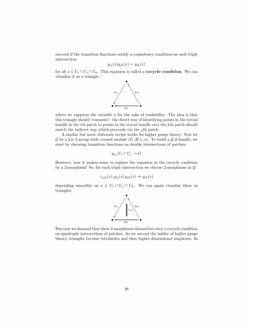
succeed if the transition functions satisfy a consistency condition on each tripleintersection:
gij(x)gjk(x) = gik(x)
for all x ∈ Ui ∩ Uj ∩ Uk. This equation is called a cocycle condition. We canvisualize it as a triangle:
•
• •gik
oo
gjk
XX
gij
where we suppress the variable x for the sake of readability. The idea is thatthis triangle should ‘commute’: the direct way of identifying points in the trivialbundle in the ith patch to points in the trivial bundle over the kth patch shouldmatch the indirect way which proceeds via the jth patch.
A similar but more elaborate recipe works for higher gauge theory. Now letG be a Lie 2-group with crossed module (G,H, t, α). To build a G-2-bundle, westart by choosing transition functions on double intersections of patches:
gij :Ui ∩ Uj → G
However, now it makes sense to replace the equation in the cocycle conditionby a 2-morphism! So, for each triple intersection we choose 2-morphisms in G:
γijk(x): gij(x) gjk(x) ⇒ gik(x)
depending smoothly on x ∈ Ui ∩ Uj ∩ Uk. We can again visualize these astriangles:
•
• •gik
oo
gjk
XX
gij
γijk
But now we demand that these 2-morphisms themselves obey a cocycle conditionon quadruple intersections of patches. As we ascend the ladder of higher gaugetheory, triangles become tetrahedra and then higher-dimensional simplexes. In
48
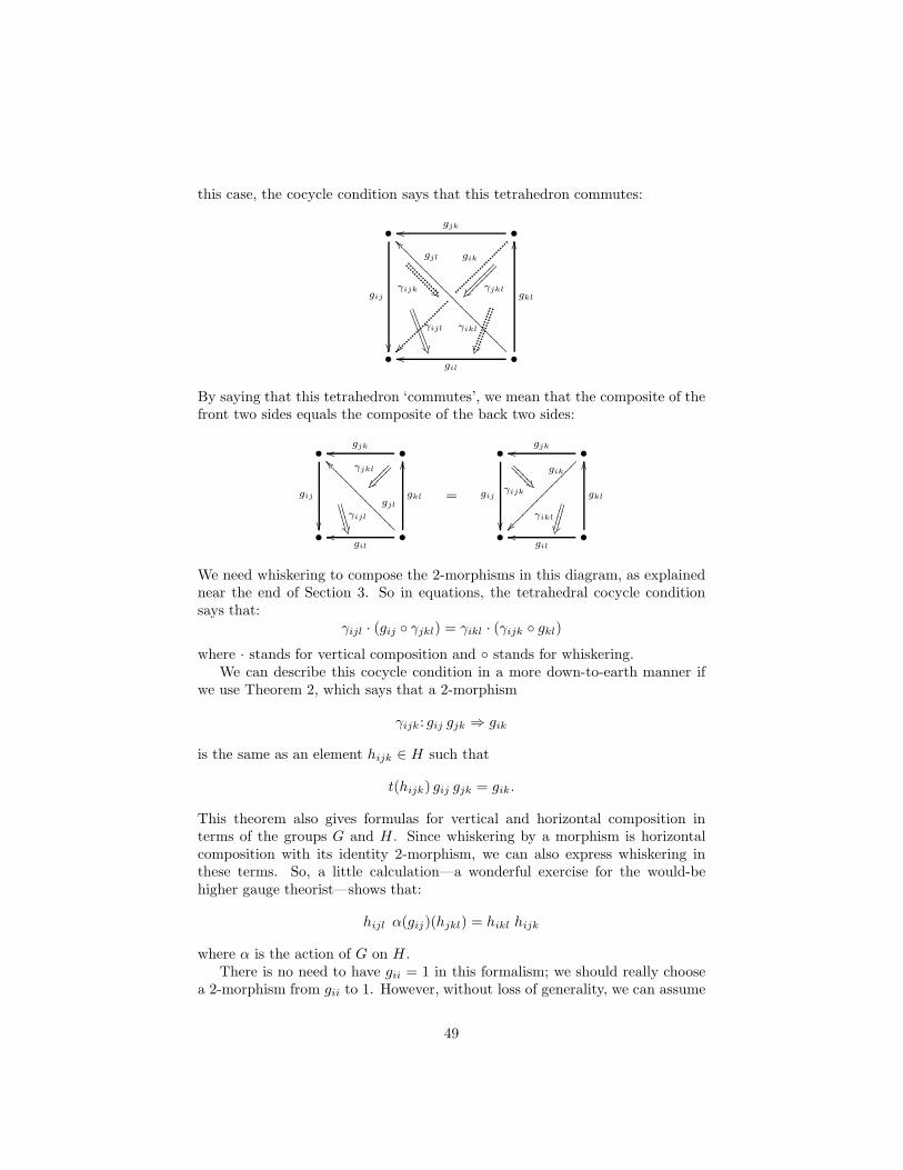
this case, the cocycle condition says that this tetrahedron commutes:
•
••
•
gkl
OOgjkoo
gij
gil
oo
gik
gjl
__γijl
γjkl ⑧⑧⑧⑧⑧⑧
⑧⑧⑧⑧⑧⑧
γijk #
γikl
By saying that this tetrahedron ‘commutes’, we mean that the composite of thefront two sides equals the composite of the back two sides:
•
••
•
gkl
OOgjkoo
gij
gil
oo
gjl
__γijl
γjkl
⑧⑧⑧⑧⑧⑧⑧⑧
=
•
••
•
gkl
OOgjkoo
gij
gil
oo⑧⑧⑧⑧⑧⑧⑧⑧⑧⑧⑧⑧⑧⑧
gik
γijk#
γikl
We need whiskering to compose the 2-morphisms in this diagram, as explainednear the end of Section 3. So in equations, the tetrahedral cocycle conditionsays that:
γijl · (gij γjkl) = γikl · (γijk gkl)
where · stands for vertical composition and stands for whiskering.We can describe this cocycle condition in a more down-to-earth manner if
we use Theorem 2, which says that a 2-morphism
γijk: gij gjk ⇒ gik
is the same as an element hijk ∈ H such that
t(hijk) gij gjk = gik.
This theorem also gives formulas for vertical and horizontal composition interms of the groups G and H . Since whiskering by a morphism is horizontalcomposition with its identity 2-morphism, we can also express whiskering inthese terms. So, a little calculation—a wonderful exercise for the would-behigher gauge theorist—shows that:
hijl α(gij)(hjkl) = hikl hijk
where α is the action of G on H .There is no need to have gii = 1 in this formalism; we should really choose
a 2-morphism from gii to 1. However, without loss of generality, we can assume
49
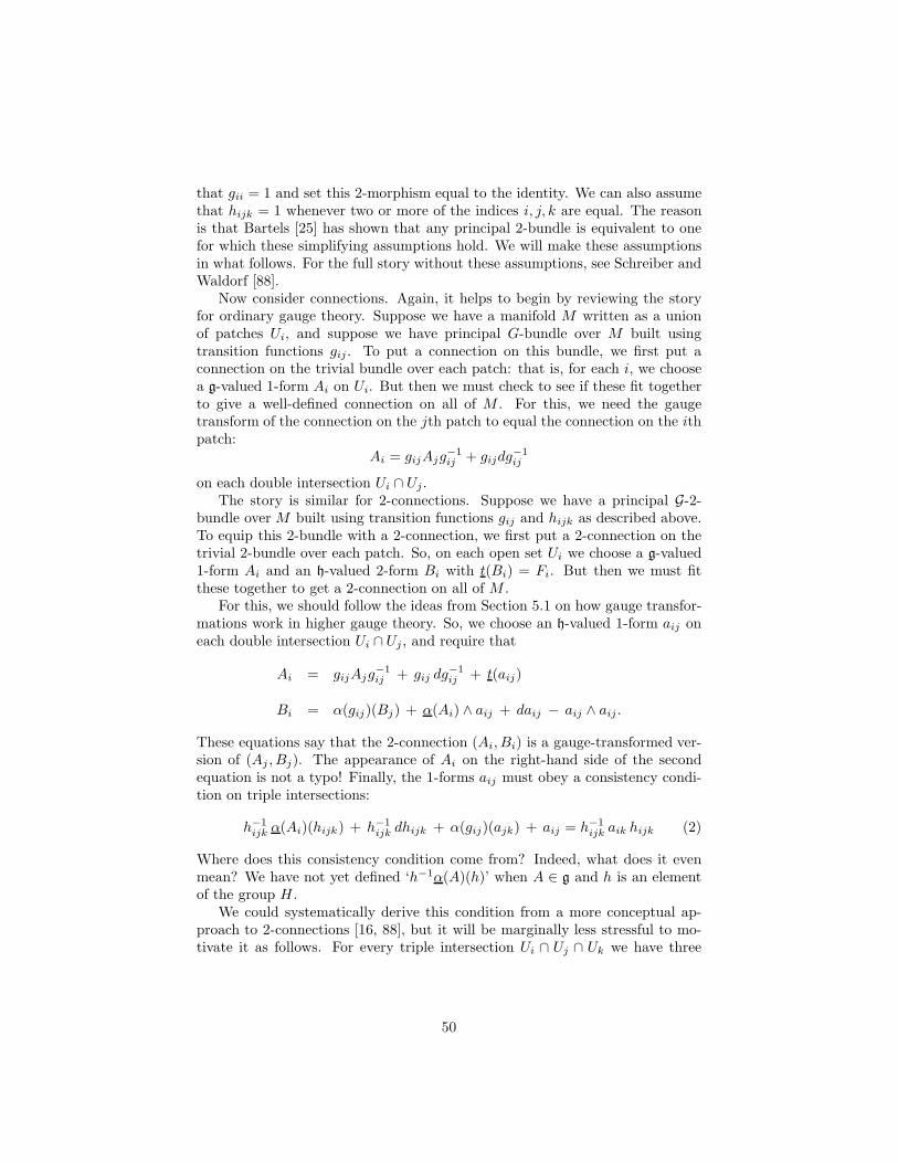
that gii = 1 and set this 2-morphism equal to the identity. We can also assumethat hijk = 1 whenever two or more of the indices i, j, k are equal. The reasonis that Bartels [25] has shown that any principal 2-bundle is equivalent to onefor which these simplifying assumptions hold. We will make these assumptionsin what follows. For the full story without these assumptions, see Schreiber andWaldorf [88].
Now consider connections. Again, it helps to begin by reviewing the storyfor ordinary gauge theory. Suppose we have a manifold M written as a unionof patches Ui, and suppose we have principal G-bundle over M built usingtransition functions gij . To put a connection on this bundle, we first put aconnection on the trivial bundle over each patch: that is, for each i, we choosea g-valued 1-form Ai on Ui. But then we must check to see if these fit togetherto give a well-defined connection on all of M . For this, we need the gaugetransform of the connection on the jth patch to equal the connection on the ithpatch:
Ai = gijAjg−1ij + gijdg
−1ij
on each double intersection Ui ∩ Uj.The story is similar for 2-connections. Suppose we have a principal G-2-
bundle over M built using transition functions gij and hijk as described above.To equip this 2-bundle with a 2-connection, we first put a 2-connection on thetrivial 2-bundle over each patch. So, on each open set Ui we choose a g-valued1-form Ai and an h-valued 2-form Bi with t(Bi) = Fi. But then we must fitthese together to get a 2-connection on all of M .
For this, we should follow the ideas from Section 5.1 on how gauge transfor-mations work in higher gauge theory. So, we choose an h-valued 1-form aij oneach double intersection Ui ∩ Uj , and require that
Ai = gijAjg−1ij + gij dg
−1ij + t(aij)
Bi = α(gij)(Bj) + α(Ai) ∧ aij + daij − aij ∧ aij .
These equations say that the 2-connection (Ai, Bi) is a gauge-transformed ver-sion of (Aj , Bj). The appearance of Ai on the right-hand side of the secondequation is not a typo! Finally, the 1-forms aij must obey a consistency condi-tion on triple intersections:
h−1ijk α(Ai)(hijk) + h−1
ijk dhijk + α(gij)(ajk) + aij = h−1ijk aik hijk (2)
Where does this consistency condition come from? Indeed, what does it evenmean? We have not yet defined ‘h−1α(A)(h)’ when A ∈ g and h is an elementof the group H .
We could systematically derive this condition from a more conceptual ap-proach to 2-connections [16, 88], but it will be marginally less stressful to mo-tivate it as follows. For every triple intersection Ui ∩ Uj ∩ Uk we have three
50
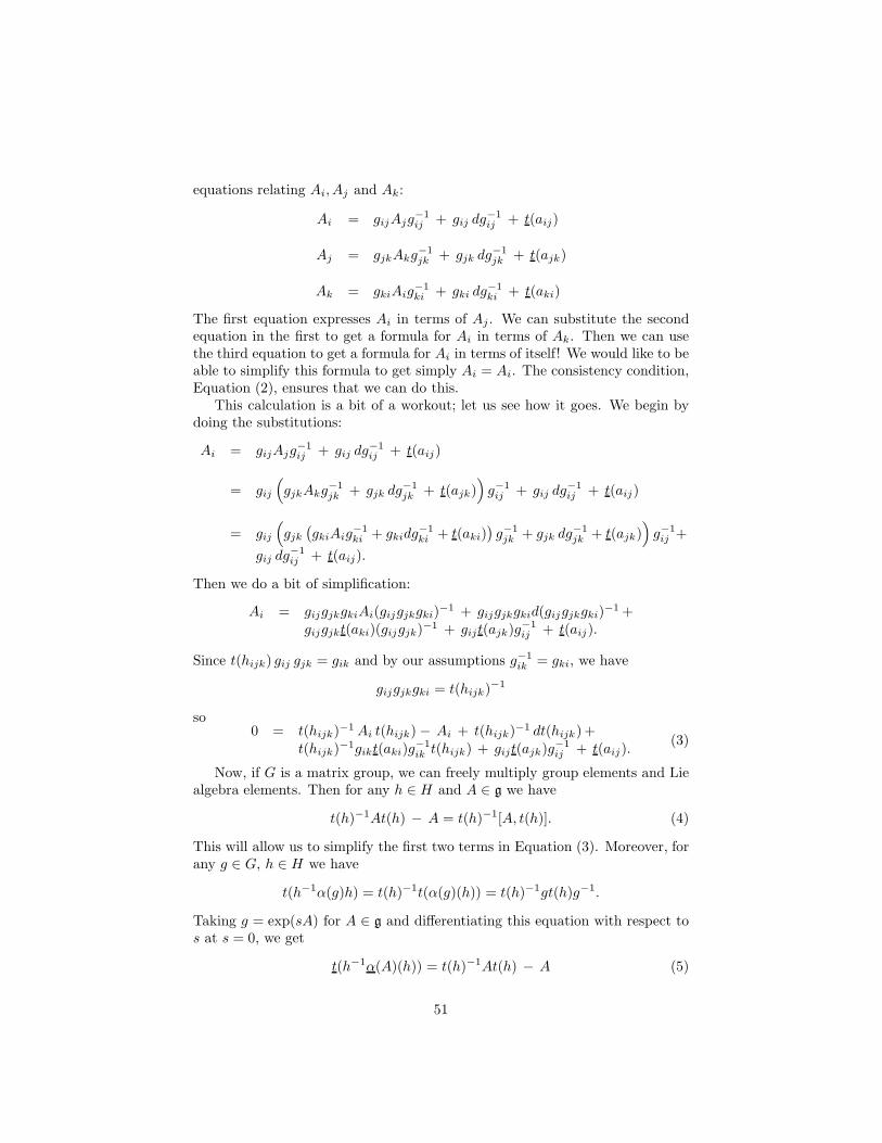
equations relating Ai, Aj and Ak:
Ai = gijAjg−1ij + gij dg
−1ij + t(aij)
Aj = gjkAkg−1jk + gjk dg
−1jk + t(ajk)
Ak = gkiAig−1ki + gki dg
−1ki + t(aki)
The first equation expresses Ai in terms of Aj . We can substitute the secondequation in the first to get a formula for Ai in terms of Ak. Then we can usethe third equation to get a formula for Ai in terms of itself! We would like to beable to simplify this formula to get simply Ai = Ai. The consistency condition,Equation (2), ensures that we can do this.
This calculation is a bit of a workout; let us see how it goes. We begin bydoing the substitutions:
Ai = gijAjg−1ij + gij dg
−1ij + t(aij)
= gij
(
gjkAkg−1jk + gjk dg
−1jk + t(ajk)
)
g−1ij + gij dg
−1ij + t(aij)
= gij
(
gjk(
gkiAig−1ki + gkidg
−1ki + t(aki)
)
g−1jk + gjk dg
−1jk + t(ajk)
)
g−1ij +
gij dg−1ij + t(aij).
Then we do a bit of simplification:
Ai = gijgjkgkiAi(gijgjkgki)−1 + gijgjkgkid(gijgjkgki)
−1 +gijgjkt(aki)(gijgjk)
−1 + gijt(ajk)g−1ij + t(aij).
Since t(hijk) gij gjk = gik and by our assumptions g−1ik = gki, we have
gijgjkgki = t(hijk)−1
so0 = t(hijk)
−1 Ai t(hijk)− Ai + t(hijk)−1 dt(hijk)+
t(hijk)−1gikt(aki)g
−1ik t(hijk) + gijt(ajk)g
−1ij + t(aij).
(3)
Now, if G is a matrix group, we can freely multiply group elements and Liealgebra elements. Then for any h ∈ H and A ∈ g we have
t(h)−1At(h) − A = t(h)−1[A, t(h)]. (4)
This will allow us to simplify the first two terms in Equation (3). Moreover, forany g ∈ G, h ∈ H we have
t(h−1α(g)h) = t(h)−1t(α(g)(h)) = t(h)−1gt(h)g−1.
Taking g = exp(sA) for A ∈ g and differentiating this equation with respect tos at s = 0, we get
t(h−1α(A)(h)) = t(h)−1At(h) − A (5)
51
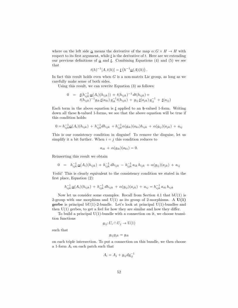
where on the left side α means the derivative of the map α:G ×H → H withrespect to its first argument, while t is the derivative of t. Here are we extendingour previous definitions of α and t. Combining Equations (4) and (5) we seethat
t(h)−1[A, t(h)] = t(
h−1α(A)(h))
.
In fact this result holds even when G is a non-matrix Lie group, as long as wecarefully make sense of both sides.
Using this result, we can rewrite Equation (3) as follows:
0 = t(h−1ijk α(Ai)(hijk)) + t(hijk)
−1 dt(hijk)+
t(hijk)−1gik t(aki) g
−1ik t(hijk) + gij t(ajk) g
−1ij + t(aij)
Each term in the above equation is t applied to an h-valued 1-form. Writingdown all these h-valued 1-forms, we see that the above equation will be true ifthis condition holds:
0 = h−1ijkα(Ai)(hijk) + h−1
ijkdhijk + h−1ijkα(gik)(aki)hijk + α(gij)(ajk) + aij
This is our consistency condition in disguise! To remove the disguise, let ussimplify it a bit further. When i = j this condition reduces to
aik + α(gik)(aki) = 0.
Reinserting this result we obtain
0 = h−1ijk α(Ai)(hijk) + h−1
ijk dhijk − h−1ijk aik hijk + α(gij)(ajk) + aij
Voila! This is clearly equivalent to the consistency condition we stated in thefirst place, Equation (2):
h−1ijk α(Ai)(hijk) + h−1
ijk dhijk + α(gij)(ajk) + aij = h−1ijk aik hijk
Now let us consider some examples. Recall from Section 4.1 that bU(1) is2-group with one morphism and U(1) as its group of 2-morphisms. A U(1)gerbe is principal bU(1)-2-bundle. Let’s look at principal U(1)-bundles andthen U(1) gerbes, to get a feel for how they are similar and how they differ.
To build a principal U(1)-bundle with a connection on it, we choose transi-tion functions
gij :Ui ∩ Uj → U(1)
such thatgijgjk = gik
on each triple intersection. To put a connection on this bundle, we then choosea 1-form Ai on each patch such that
Ai = Aj + gijdg−1ij
52
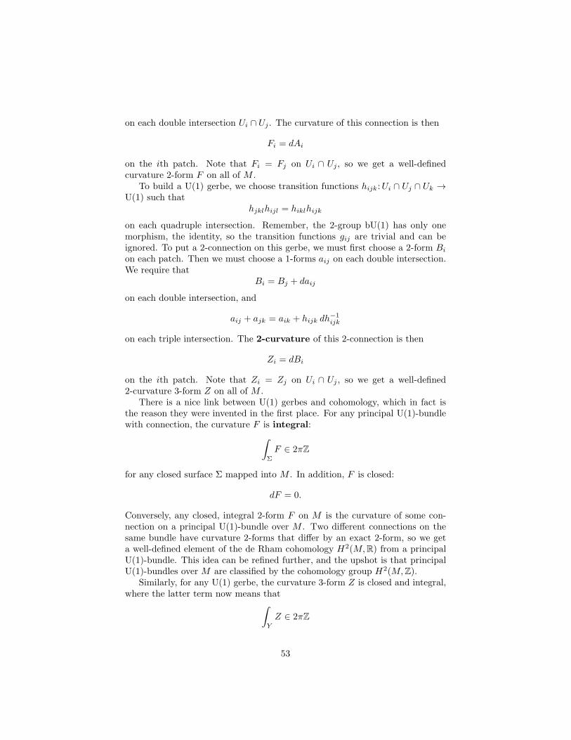
on each double intersection Ui ∩ Uj. The curvature of this connection is then
Fi = dAi
on the ith patch. Note that Fi = Fj on Ui ∩ Uj, so we get a well-definedcurvature 2-form F on all of M .
To build a U(1) gerbe, we choose transition functions hijk:Ui ∩ Uj ∩ Uk →U(1) such that
hjklhijl = hiklhijk
on each quadruple intersection. Remember, the 2-group bU(1) has only onemorphism, the identity, so the transition functions gij are trivial and can beignored. To put a 2-connection on this gerbe, we must first choose a 2-form Bi
on each patch. Then we must choose a 1-forms aij on each double intersection.We require that
Bi = Bj + daij
on each double intersection, and
aij + ajk = aik + hijk dh−1ijk
on each triple intersection. The 2-curvature of this 2-connection is then
Zi = dBi
on the ith patch. Note that Zi = Zj on Ui ∩ Uj , so we get a well-defined2-curvature 3-form Z on all of M .
There is a nice link between U(1) gerbes and cohomology, which in fact isthe reason they were invented in the first place. For any principal U(1)-bundlewith connection, the curvature F is integral:
∫
Σ
F ∈ 2πZ
for any closed surface Σ mapped into M . In addition, F is closed:
dF = 0.
Conversely, any closed, integral 2-form F on M is the curvature of some con-nection on a principal U(1)-bundle over M . Two different connections on thesame bundle have curvature 2-forms that differ by an exact 2-form, so we geta well-defined element of the de Rham cohomology H2(M,R) from a principalU(1)-bundle. This idea can be refined further, and the upshot is that principalU(1)-bundles over M are classified by the cohomology group H2(M,Z).
Similarly, for any U(1) gerbe, the curvature 3-form Z is closed and integral,where the latter term now means that
∫
Y
Z ∈ 2πZ
53
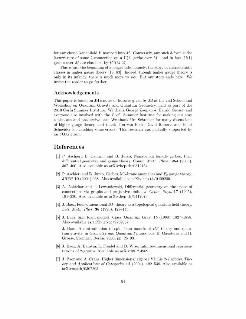
for any closed 3-manifold Y mapped into M . Conversely, any such 3-form is the2-curvature of some 2-connection on a U(1) gerbe over M—and in fact, U(1)gerbes over M are classified by H3(M,Z).
This is just the beginning of a longer tale: namely, the story of characteristicclasses in higher gauge theory [18, 83]. Indeed, though higher gauge theory isonly in its infancy, there is much more to say. But our story ends here. Weinvite the reader to go further.
Acknowledgements
This paper is based on JH’s notes of lectures given by JB at the 2nd School andWorkshop on Quantum Gravity and Quantum Geometry, held as part of the2010 Corfu Summer Institute. We thank George Zoupanos, Harald Grosse, andeveryone else involved with the Corfu Summer Institute for making our staya pleasant and productive one. We thank Urs Schreiber for many discussionsof higher gauge theory, and thank Tim van Beek, David Roberts and ElliotSchneider for catching some errors. This research was partially supported byan FQXi grant.
References
[1] P. Aschieri, L. Cantini, and B. Jurco, Nonabelian bundle gerbes, theirdifferential geometry and gauge theory, Comm. Math. Phys. 254 (2005),367–400. Also available as arXiv:hep-th/0312154.
[2] P. Aschieri and B. Jurco, Gerbes, M5-brane anomalies and E8 gauge theory,JHEP 10 (2004) 068. Also available as arXiv:hep-th/0409200.
[3] A. Ashtekar and J. Lewandowski, Differential geometry on the space ofconnections via graphs and projective limits, J. Geom. Phys. 17 (1995),191–230. Also available as arXiv:hep-th/9412073.
[4] J. Baez, Four-dimensional BF theory as a topological quantum field theory,Lett. Math. Phys. 38 (1996), 129–143.
[5] J. Baez, Spin foam models, Class. Quantum Grav. 15 (1998), 1827–1858.Also available as arXiv:gr-qc/9709052.
J. Baez, An introduction to spin foam models of BF theory and quan-tum gravity, in Geometry and Quantum Physics, eds. H. Gausterer and H.Grosse, Springer, Berlin, 2000, pp. 25–93.
[6] J. Baez, A. Baratin, L. Freidel and D. Wise, Infinite-dimensional represen-tations of 2-groups. Available as arXiv:0812.4969.
[7] J. Baez and A. Crans, Higher dimensional algebra VI: Lie 2-algebras, The-ory and Applications of Categories 12 (2004), 492–538. Also available asarXiv:math/0307263.
54
[8] J. Baez, A. Crans, U. Schreiber and D. Stevenson From loop groups to 2-groups, HHA 9 (2007), 101–135. Also available as arXiv:math.QA/0504123.
[9] J. Baez, A. Crans and D. Wise, Exotic statistics for strings in 4d BFtheory, Adv. Theor. Math. Phys. 11 (2007), 707–749. Also available asarXiv:gr-qc/0603085.
[10] J. Baez, A. Hoffnung, C. Rogers, Categorified symplectic geometry and theclassical string, Comm. Math. Phys. 293 (2010), 701–715. Also availableas arXiv:0808.0246.
[11] J. Baez and J. Huerta, Division algebras and supersymmetry II. Availableas arXiv:1003.3436.
[12] J. Baez and A. Lauda, A prehistory of n-categorical physics. Available asarXiv:0908.2469.
[13] J. Baez and A. Lauda, Higher dimensional algebra V: 2-groups, The-ory and Applications of Categories 12 (2004), 423–491. Also available asarXiv:math/0307200.
[14] J. Baez and A. Perez, Quantization of strings and branes coupled toBF theory, Adv. Theor. Math. Phys. 11 (2007), 1–19. Also available asarXiv:gr-qc/0605087.
[15] J. Baez and C. Rogers, Categorified symplectic geometry and the string Lie2-algebra, to appear in Homology, Homotopy and Applications. Availableas arXiv:0901.4721.
[16] J. Baez and U. Schreiber, Higher gauge theory, in Categories in Al-gebra, Geometry and Mathematical Physics, eds. A. Davydov et al,Contemp. Math. 431, AMS, Providence, 2007, pp. 7–30. Also availablearXiv:math/0511710.
[17] J. Baez and S. Sawin, Functional integration on spaces of connections, J.Funct. Analysis 150 (1997), 1-26. Also available as arXiv:q-alg/9507023.
[18] J. Baez and D. Stevenson, The classifying space of a topological 2-group,in Algebraic Topology: The Abel Symposium 2007, eds. Nils Baas, EricFriedlander, Bjørn Jahren and Paul Arne Østvær, Springer, Berlin, 2009.
[19] I. Bakovic and B. Jurco, The classifying topos of a topological bicategory.Available as arXiv:0902.1750.
[20] A. P. Balachandran, F. Lizzi and G. Sparano, A new approach to stringsand superstrings, Nucl. Phys. B277 (1986), 359-387.
[21] A. Baratin and L. Freidel, Hidden quantum gravity in 3d Feynman di-agrams, Class. Quant. Grav. 24 (2007), 1993–2026. Also available asarXiv:gr-qc/0604016.
55
[22] A. Baratin and L. Freidel, Hidden quantum gravity in 4d Feynman dia-grams: emergence of spin foams, Class. Quant. Grav. 24 (2007), 2027–2060.Also available as arXiv:hep-th/0611042.
[23] A. Baratin and D. Wise, 2-Group representations for spin foams. Availableas arXiv:0910.1542.
[24] J. W. Barrett and M. Mackaay, Categorical representations of cate-gorical groups, Th. Appl. Cat. 16 (2006), 529–557 Also available asarXiv:math/0407463.
[25] T. Bartels, Higher gauge theory: 2-bundles. Available asarXiv:math.CT/0410328.
[26] Jean Benabou, Introduction to bicategories, in Reports of the MidwestCategory Seminar, Springer, Berlin, 1967, pp. 1–77.
[27] F. Borceux, Handbook of Categorical Algebra 1: Basic Category Theory,Cambridge U. Press, Cambridge, 1994.
[28] L. Breen, Notes on 1- and 2-gerbes, in Towards Higher Categories, eds. J.Baez and P. May, Springer, Berlin, 2009, pp. 193–235. Also available asarXiv:math/0611317.
[29] L. Breen, Differential geometry of gerbes and differential forms. Availableas arXiv:0802.1833.
[30] L. Breen and W. Messing, Differential geometry of gerbes, Adv. Math. 198(2005), 732–846. Available as arXiv:math.AG/0106083.
[31] J.-L. Brylinski, Loop Spaces, Characteristic Classes and Geometric Quan-tization, Birkhauser, Boston, 1993.
[32] J.-L. Brylinski, Differentiable cohomology of gauge groups. Available asarXiv:math.DG/0011069.
[33] J.-L. Brylinski and D. A. McLaughlin, The geometry of degree-four char-acteristic classes and of line bundles on loop spaces I, Duke Math. J. 75(1994), 603–638.
J.-L. Brylinski and D. A. McLaughlin, The geometry of degree-four char-acteristic classes and of line bundles on loop spaces II, Duke Math. J. 83(1996), 105–139.
[34] A. L. Carey, S. Johnson and M. K. Murray, Holonomy on D-branes, Jour.Geom. Phys. 52 (2004), 186–216. Also available as arXiv:hep-th/0204199.
[35] L. Crane, L. Kauffman and D. Yetter, State-sum invariants of 4-manifoldsI. Available as arXiv:hep-th/9409167.
[36] L. Crane and M. D. Sheppeard, 2-Categorical Poincare representations andstate sum applications, available as arXiv:math/0306440.
56
[37] L. Crane and D. Yetter, A categorical construction of 4d TQFTs, in Quan-tum Topology, eds. L. Kauffman and R. Baadhio, World Scientific, Singa-pore, 1993, pp. 120-130. Also available as arXiv:hep-th/9301062.
[38] L. Crane and D. N. Yetter, Measurable categories and 2-groups, Appl. Cat.Str. 13 (2005), 501–516. Also available as arXiv:math/0305176.
[39] T. DeDonder, Theorie Invariantive du Calcul des Variations, Gauthier–Villars, Paris, 1935.
[40] C. DeWitt-Morette, A. Maheshwari, and B. Nelson, Path integration inphase space, Gen. Relativity Gravitation 8 (1977), 581–593.
[41] L. Castellani, R. D’Auria and P. Fre, Supergravity and Superstrings: AGeometric Perspective, World Scientific, Singapore, 1991.
[42] M. J. Duff, Supermembranes: the first fifteen weeks, Class. Quantum Grav.
5 (1988), 189–205. Also available at〈http://www-lib.kek.jp/cgi-bin/img index?8708425〉.
[43] B. Eckmann and P. Hilton, Group-like structures in categories, Math. Ann.145 (1962), 227-255.
[44] S. Eilenberg and S. Mac Lane, General theory of natural equivalences,Trans. Amer. Math. Soc. 58 (1945), 231–294.
[45] C. Ehresmann, Categories topologiques et categories differentiables, Coll.Geom. Diff. Globale (Bruxelles, 1958), Centre Belge Rech. Math. Louvain,1959, pp. 137–150.
[46] C. Ehresmann, Categories structurees, Ann. Ecole Norm. Sup. 80 (1963),349–426.
[47] C. Ehresmann, Categories et Structures, Dunod, Paris, 1965.
[48] J. Elgueta, Representation theory of 2-groups on Kapranov and Voevod-sky 2-vector spaces, Adv. Math. 213 (2007), 53–92. Also available asarXiv:math/0408120.
[49] W. Fairbairn and A. Perez, Extended matter coupled to BF theory, Adv.Theor. Math. Phys. D78:024013 (2008). Also available as arXiv:0709.4235.
[50] W. Fairbairn, K. Noui and F. Sardelli, Canonical analysis of algebraic stringactions. Available as arXiv:0908.0953.
[51] M. Forrester-Barker, Group objects and internal categories, available asarXiv:math.CT/0212065.
[52] D. S. Freed and E. Witten, Anomalies in string theory with D-Branes, §6:Additional remarks, Asian J. Math. 3 (1999) 819–852. Also available asarXiv:hep-th/9907189.
57
[53] L. Freidel and D. Louapre: Ponzano–Regge model revisited. I: Gauge fix-ing, observables and interacting spinning particles, Class. Quant. Grav. 21(2004), 5685–5726. Also available as arXiv:hep-th/0401076.
L. Freidel and D. Louapre: Ponzano–Regge model revisited. II: Equivalencewith Chern–Simons. Also available as arXiv:gr-qc/0410141.
L. Freidel and E. Livine: Ponzano–Regge model revisited. III: Feynmandiagrams and effective field theory. Also available as arXiv:hep-th/0502106.
[54] K. Gawedzki, Topological actions in two-dimensional quantum field theo-ries, in Nonperturbative Quantum Field Theory, eds. G. t’Hooft, A. Jaffe,G. Mack P. K. Mitter and R. Stora, Plenum, New York, 1988, pp. 101–141.
[55] K. Gawedzki and N. Reis, WZW branes and gerbes, Rev. Math. Phys. 14(2002), 1281–1334. Also available as arXiv:hep-th/0205233.
[56] E. Getzler, Lie theory for nilpotent L∞-algebras. Available asarXiv:math/0404003.
[57] M. Gotay, J. Isenberg, J. Marsden, and R. Montgomery, Momentum mapsand classical relativistic fields. Part I: covariant field theory, available asarXiv:physics/9801019.
[58] F. Girelli and H. Pfeiffer, Higher gauge theory - differential versus integralformulation, Jour. Math. Phys. 45 (2004), 3949–3971. Also available asarXiv:hep-th/0309173.
[59] F. Girelli, H. Pfeiffer and E. M. Popescu, Topological higher gauge theory -from BF to BFCG theory, J. Math. Phys. 49:032503, 2008. Also availableas arXiv:0708.3051.
[60] V. Guillemin and S. Sternberg, Symplectic Techniques in Physics, Cam-bridge U. Press, Cambridge, 1984.
[61] A. Henriques, Integrating L∞-algebras. Available as arXiv:math/0603563.
[62] M. Johnson, The combinatorics of n-categorical pasting, Jour. Pure Appl.Alg. 62 (1989), 211–225.
[63] S. Lack, A 2-categories companion, in Towards Higher Categories, eds.J. Baez and P. May, Springer, 2009, pp. 105–191. Also available asarXiv:math/0702535.
[64] E. Lerman, Orbifolds as stacks?, available as arXiv:0806.4160.
[65] J. Lewandowski and T. Thiemann, Diffeomorphism invariant quantum fieldtheories of connections in terms of webs, Class. Quant. Grav. 16 (1999),2299–2322. Also available as arXiv:gr-qc/9901015.
[66] S. Mac Lane and J. H. C. Whitehead, On the 3-type of a complex, Proc.Nat. Acad. Sci. 36 (1950), 41–48.
58
[67] M. Mackaay and R. Picken, Holonomy and parallel transport forAbelian gerbes, Adv. Math. 170 (2002), 287–339. Also available asarXiv:math.DG/0007053.
[68] M. Markl, S. Schnider and J. Stasheff, Operads in Algebra, Topology andPhysics, AMS, Providence, Rhode Island, 2002.
[69] J. F. Martins and R. Picken, On two-dimensional holonomy. Available asarXiv:0710.4310.
J. F. Martins and R. Picken, A cubical set approach to 2-bundles withconnection and Wilson surfaces. Available as arXiv:0808.3964.
[70] J. F. Martins and R. Picken, The fundamental Gray 3-groupoid of a smoothmanifold and local 3-dimensional holonomy based on a 2-crossed module.Available as arXiv:0907.2566
[71] J. Milnor, Remarks on infinite dimensional Lie groups, Relativity, Groupsand Topology II, (Les Houches, 1983), North-Holland, Amsterdam, 1984.
[72] I. Moerdijk, Introduction to the language of stacks and gerbes. Availableas arXiv:math.AT/0212266.
[73] M. Montesinos and A. Perez, Two-dimensional topological field theoriescoupled to four-dimensional BF theory, Phys. Rev. D77:104020 (2008).Also available as arXiv:0709.4235.
[74] M. K. Murray, Bundle gerbes, J. London Math. Soc. 54 (1996), 403–416.Also available as arXiv:dg-ga/9407015.
M. K. Murray, An introduction to bundle gerbes. Available asarXiv:0712.1651.
[75] M. K. Murray and D. Stevenson, Higgs fields, bundle gerbes and stringstructures, Commun. Math. Phys. 243 (2003), 541–555. Also available asarXiv:math.DG/0106179.
[76] H. Pfeiffer, Higher gauge theory and a non-Abelian generalization of 2-form electromagnetism, Ann. Phys. 308 (2003), 447–477. Also availableas arXiv:hep-th/0304074.
[77] A. J. Power, A 2-categorical pasting theorem, Jour. Alg. 129 (1990), 439-445.
[78] A. Pressley and G. Segal, Loop Groups, Oxford U. Press, Oxford, 1986.
[79] D. Roberts and U. Schreiber, The inner automorphism 3-group of a strict2-group. Also available as arXiv:0708.1741.
[80] C. Rovelli, Quantum Gravity, Cambridge U. Press, 2004. Also available at〈http://www.cpt.univ-mrs.fr/∼rovelli/book.pdf〉.
59
[81] D. Roytenberg, On weak Lie 2-algebras. Available as arXiv:0712.3461.
[82] H. Sati, Geometric and topological structures related to M-branes. Avail-able as arXiv:1001.5020.
[83] H. Sati, U. Schreiber and J. Stasheff, L∞-algebras and applications tostring- and Chern–Simons n-transport. Available as arXiv:0801.3480.
[84] M. Schlessinger and J. Stasheff, The Lie algebra structure of tangent coho-mology and deformation theory, Jour. Pure App. Alg. 38 (1985), 313–322.
[85] C. Schommer-Pries, A finite-dimensional string 2-group. Available asarXiv:0911.2483.
[86] U. Schreiber, comments at the n-Category Cafe. Available at〈http://golem.ph.utexas.edu/category/2009/09/questions on ncurvature.html〉.
[87] U. Schreiber and K. Waldorf, Parallel transport and functors, J. HomotopyRelat. Struct. 4 (2009), 187–244. Also available as arXiv:0705.0452.
[88] U. Schreiber and K. Waldorf, Smooth functors vs. differential forms. Avail-able as arXiv:0802.0663.
U. Schreiber and K. Waldorf, Connections on non-abelian gerbes and theirholonomy. Available as arXiv:0808.1923.
[89] D. Stevenson, The Geometry of Bundle Gerbes, Ph.D. thesis, University ofAdelaide, 2000. Also available as arXiv:math.DG/0004117.
[90] S. Stolz and P. Teichner, What is an elliptic object?, in Topology, Geometryand Quantum Field Theory: Proceedings of the 2002 Oxford Symposium inHonour of the 60th Birthday of Graeme Segal, ed. U. Tillmann, CambridgeU. Press, Cambridge, 2004.
[91] K. Waldorf, String connections and Chern–Simons theory. Available asarXiv:0906.0117.
[92] H. Weyl, Geodesic fields in the calculus of variation for multiple integrals,Ann. Math. 36 (1935), 607–629.
[93] J. H. C. Whitehead, Note on a previous paper entitled ‘On adding relationsto homotopy groups’, Ann. Math. 47 (1946), 806–810.
J. H. C. Whitehead, Combinatorial homotopy II, Bull. Amer. Math. Soc.55 (1949), 453–496
[94] E. Witten, The index of the Dirac operator in loop space, in Elliptic Curvesand Modular Forms in Algebraic Topology, ed. P. S. Landweber, LectureNotes in Mathematics 1326, Springer, Berlin, 1988, pp. 161–181.
60


![q-Deformationsand t-DeformationsoftheMarkovtriplesarXiv:2008.12913v3 [math.NT] 4 Oct 2020 q-Deformationsandt-DeformationsoftheMarkovtriples TakeyoshiKogiso DepartmentofMathematics,JosaiUniversity,](https://img.pdfslide.net/doc/110x75/60812b2da1e52a483b667f13/q-deformationsand-t-deformationsofthemarkovtriples-arxiv200812913v3-mathnt.jpg)


![Divya Goel DepartmentofMathematics ...arXiv:1804.08084v2 [math.AP] 31 May 2018 CoronproblemfornonlocalequationsinvlovingChoquard nonlinearity Divya Goel∗ and K. Sreenadh† DepartmentofMathematics](https://img.pdfslide.net/doc/110x75/5f49b8323ac3aa147a521810/divya-goel-departmentofmathematics-arxiv180408084v2-mathap-31-may-2018.jpg)