Embed Size (px)
Citation preview

Joint, Conditional, & Marginal Probabilities
Statistics 110
Summer 2006
Copyright c©2006 by Mark E. Irwin

Joint, Conditional, & Marginal Probabilities
The three axioms for probability don’t discuss how to create probabilitiesfor combined events such as P [A ∩ B] or for the likelihood of an event Agiven that you know event B occurs.
Example:
Let A be the event it rains today and B be the event that it rains tomorrow.Does knowing about whether it rains today change our belief that it willrain tomorrow. That is, is P [B], the probability that it rains tomorrowignoring information on whether it rains today, different from P [B|A], theprobability that it rains tomorrow given that it rains today.
P [B|A] is known as the conditional probability of B given A.
It is quite likely that P [B] and P [B|A] are different.
Joint, Conditional, & Marginal Probabilities 1

Example: ELISA (Enzyme-Linked Immunosorbent Assay) test for HIV
ELISA is a common screening test for HIV. However it is not perfect as
P [+test|HIV] = 0.98
P [−test|Not HIV] = 0.93
So for people with HIV infections, 98% of them have positive tests(sensitivity), whereas people without HIV infections, 93% of them havenegative tests (specificity).
These give the two error rates
P [−test|HIV] = 0.02 = 1− P [+test|HIV]
P [+test|Not HIV] = 0.07 = 1− P [−test|Not HIV]
(Note: the complement rule holds for conditional probabilities)
When this test was evaluated in the early 90s, for a randomly selectedAmerican, P [HIV] = 0.01
Joint, Conditional, & Marginal Probabilities 2

The question of real interest is what are
P [HIV|+test]
P [Not HIV|−test]
To figure these out, we need a bit more information.
Joint, Conditional, & Marginal Probabilities 3

Definition:
Let A and B be two events with P [B] > 0.The conditional probability of A given B isdefined to be
P [A|B] =P [A ∩B]
P [B]
One way to think about this is that if weare told that event B occurs, the samplespace of interest is now B instead of Ω andconditional probability is a probability measure on B.
Joint, Conditional, & Marginal Probabilities 4
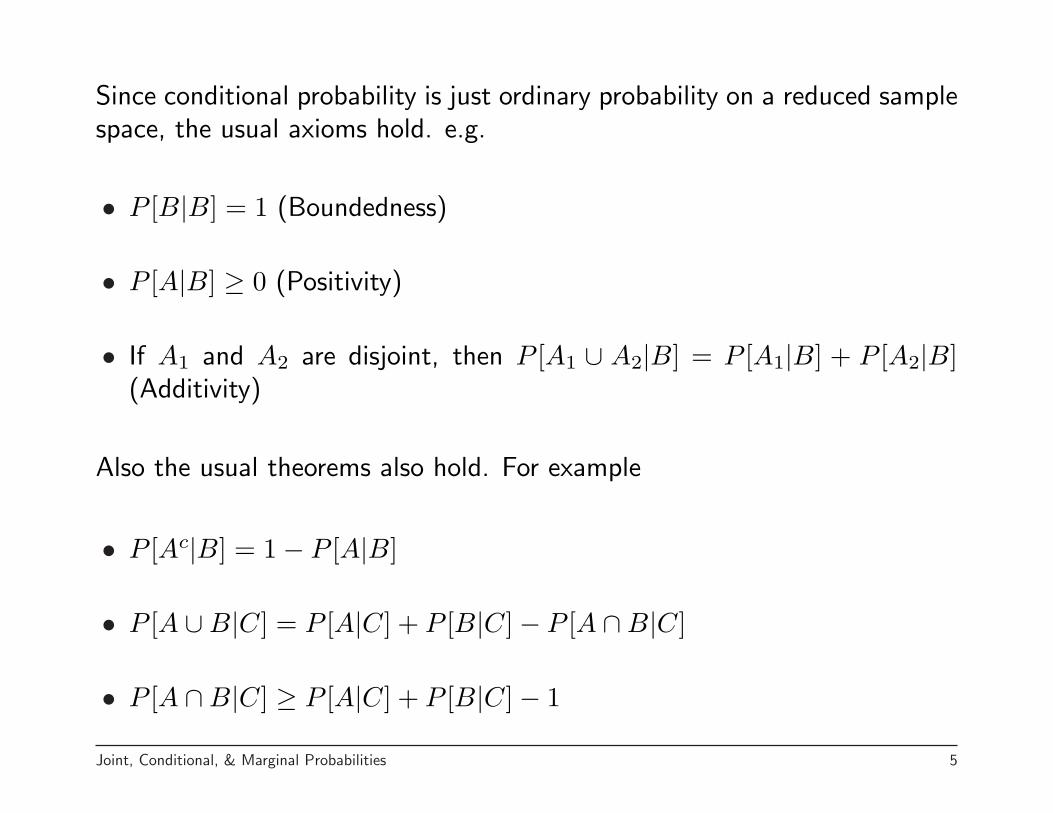
Since conditional probability is just ordinary probability on a reduced samplespace, the usual axioms hold. e.g.
• P [B|B] = 1 (Boundedness)
• P [A|B] ≥ 0 (Positivity)
• If A1 and A2 are disjoint, then P [A1 ∪ A2|B] = P [A1|B] + P [A2|B](Additivity)
Also the usual theorems also hold. For example
• P [Ac|B] = 1− P [A|B]
• P [A ∪B|C] = P [A|C] + P [B|C]− P [A ∩B|C]
• P [A ∩B|C] ≥ P [A|C] + P [B|C]− 1
Joint, Conditional, & Marginal Probabilities 5

We can use the definition of conditional probability to get
Multiplication Rule:
Let A and B be events. Then
P [A ∩B] = P [A|B]P [B]
Also the relationship also holds with the other ordering, i.e.
P [A ∩B] = P [B|A]P [A]
Note that P [A ∩ B] is sometimes known as the joint probability of A andB.
Back to ELISA example
To get P [HIV|+test] and P [Not HIV|−test] we need the followingquantities
P [HIV ∩+test], P [Not HIV ∩ −test], P [+test], P [−test]
Joint, Conditional, & Marginal Probabilities 6

The joint probabilities can be calculated using the multiplication rule
P [HIV ∩+test] = P [HIV]P [+test|HIV] = 0.01× 0.98 = 0.0098
P [HIV ∩ −test] = P [HIV]P [−test|HIV] = 0.01× 0.02 = 0.0002
P [Not HIV ∩+test] = P [Not HIV]P [+test|Not HIV]
= 0.99× 0.07 = 0.0693
P [Not HIV ∩ −test] = P [Not HIV]P [−test|Not HIV]
= 0.99× 0.93 = 0.9207
The marginal probabilities on test status are
P [+test] = P [HIV ∩+test] + P [Not HIV ∩+test]
= 0.0098 + 0.0693 = 0.0791
P [−test] = P [HIV ∩ −test] + P [Not HIV ∩ −test]
= 0.0002 + 0.9207 = 0.9209
Joint, Conditional, & Marginal Probabilities 7

It is often convenient to display the joint and marginal probabilities in a 2way table as follows
HIV Not HIV
+Test 0.0098 0.0693 0.0791
–Test 0.0002 0.9207 0.9209
0.0100 0.9900 1.0000
Note that the calculation of the test status probabilities is an example ofthe Law of Total Probability
Law of Total Probability:Let B1, B2, . . . , Bn be such that
⋃ni=1 Bi = Ω and Bi ∩ Bj for i 6= j with
P [Bi] > 0 for all i. Then for any event A,
P [A] =n∑
i=1
P [A|Bi]P [Bi]
Joint, Conditional, & Marginal Probabilities 8

Proof
P [A] = P [A ∩ Ω]
= P
[A ∩
(n⋃
i=1
Bi
)]
= P
[n⋃
i=1
(A ∩Bi)
]
Since the events A ∩Bi are disjoint
P
[n⋃
i=1
(A ∩Bi)
]=
n∑
i=1
P [A ∩Bi]
=n∑
i=1
P [A|Bi]P [Bi]
Joint, Conditional, & Marginal Probabilities 9

Note: If a set of events Bi satisfy the conditions above, they are said toform a partition of the sample space.
One way to think of this theorem is to find the probability of A, we cansum the conditional probabilities of A given Bi, weighted by P [Bi].
Now we can get the two desired conditional probabilities.
P [HIV|+test] =P [HIV ∩+test]
P [+test]=
0.00980.0791
= 0.124
P [Not HIV|−test] =P [Not HIV ∩ −test]
P [−test]=
0.92070.9209
= 0.99978
These numbers may appear surprising. What is happening here is that mostof the people that have positive test are actually uninfected and they areswamping out the the people that actually are infected.
One key thing to remember that P [A|B] and P [B|A] are completelydifferent things. In the example P [HIV|+test] and P [+test|HIV] aredescribing two completely different concepts.
Joint, Conditional, & Marginal Probabilities 10
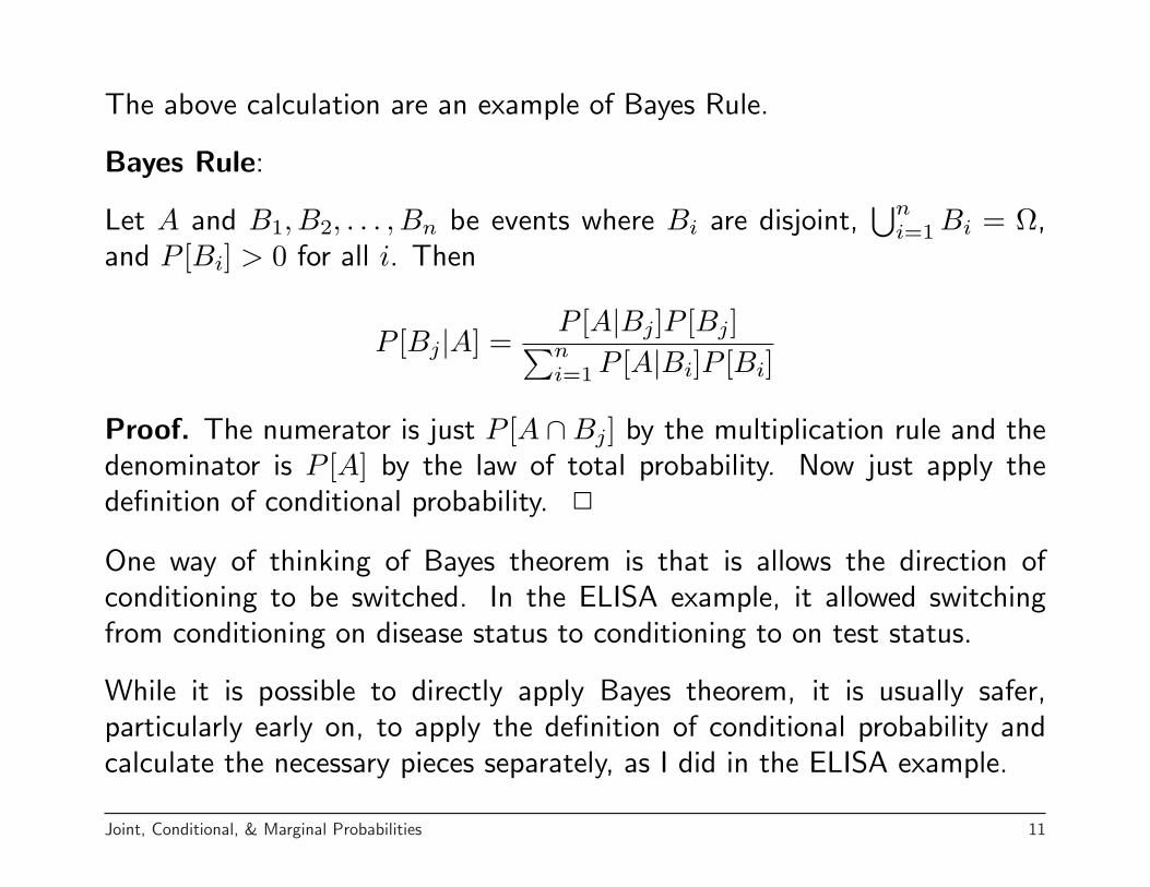
The above calculation are an example of Bayes Rule.
Bayes Rule:
Let A and B1, B2, . . . , Bn be events where Bi are disjoint,⋃n
i=1 Bi = Ω,and P [Bi] > 0 for all i. Then
P [Bj|A] =P [A|Bj]P [Bj]∑ni=1 P [A|Bi]P [Bi]
Proof. The numerator is just P [A ∩Bj] by the multiplication rule and thedenominator is P [A] by the law of total probability. Now just apply thedefinition of conditional probability. 2
One way of thinking of Bayes theorem is that is allows the direction ofconditioning to be switched. In the ELISA example, it allowed switchingfrom conditioning on disease status to conditioning to on test status.
While it is possible to directly apply Bayes theorem, it is usually safer,particularly early on, to apply the definition of conditional probability andcalculate the necessary pieces separately, as I did in the ELISA example.
Joint, Conditional, & Marginal Probabilities 11

There is another way of looking at Bayes theorem. Instead of probabilities,we can look at odds. An equivalent statement is
P [Bi|A]P [Bj|A]︸ ︷︷ ︸
Posterior Odds
=P [A|Bi]P [A|Bj]︸ ︷︷ ︸
Likelihood Ratio
× P [Bi]P [Bj]︸ ︷︷ ︸
Prior Odds
This approach is useful when B1, B2, . . . , Bn is a set of competinghypotheses and A is information (data) that we want to use to try tohelp pick the correct hypothesis.
This suggests another way of thinking of Bayes theorem. It tells us how toupdate probabilities in the presence of new evidence.
Joint, Conditional, & Marginal Probabilities 12

Who is this man?
This is reportedly the only known picture ofthe Reverend Thomas Bayes, F.R.S. — 1701?- 1761.
This picture was taken from the 1936 Historyof Life Insurance (by Terence O’Donnell,American Conservation Co., Chicago). Asno source is given, the authenticity of thisportrait is open to question.
So what is the probability that this is actuallyReverend Thomas Bayes?
However there is some additional information.How does this change our belief about whothis is?
Who is this man? 13
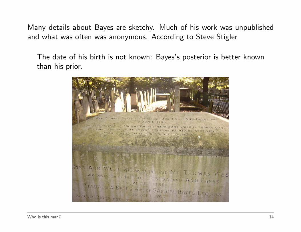
Many details about Bayes are sketchy. Much of his work was unpublishedand what was often was anonymous. According to Steve Stigler
The date of his birth is not known: Bayes’s posterior is better knownthan his prior.
Who is this man? 14

Actually his date of death isn’t that well known either. Its general consideredto be April 7, 1761 however it has also be reported as April 17th of thesame year.
There is some additional information we can get from this picture to helpuse decide whether this is Bayes or not.
1. The caption under the photo in O’Donnell’s book was “Rev. T. Bayes:Improver of the Columnar Method developed by Barrett”.
There are some problems with this claim. First Barrett was born in 1752and would have been about 9 years old when Bayes died. In addition, themethod that Bayes allegedly improved was apparently developed between1788 and 1811 and read to the Royal Society in 1812, long after Bayes’death.
So there is a problem here, but whether it is a problem with just thecaption or the picture as well isn’t clear.
Who is this man? 15
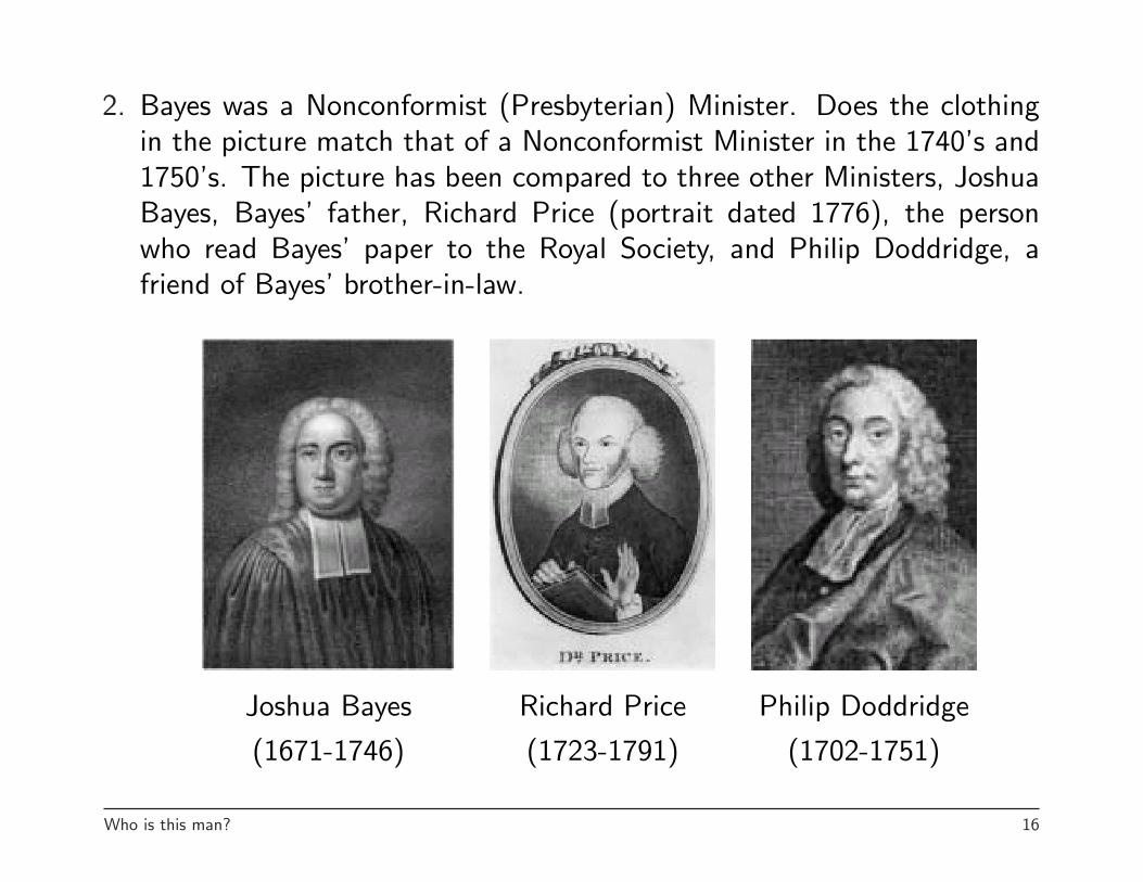
2. Bayes was a Nonconformist (Presbyterian) Minister. Does the clothingin the picture match that of a Nonconformist Minister in the 1740’s and1750’s. The picture has been compared to three other Ministers, JoshuaBayes, Bayes’ father, Richard Price (portrait dated 1776), the personwho read Bayes’ paper to the Royal Society, and Philip Doddridge, afriend of Bayes’ brother-in-law.
Joshua Bayes Richard Price Philip Doddridge
(1671-1746) (1723-1791) (1702-1751)
Who is this man? 16

Two things stand out in the comparisons.
(a) No wig. It is likely that Bayes should have been wearing a wig similarto Doddridge’s, which was going out of fashion in the 1740’s or similarto Price’s, which was coming into style at the time.
(b) Bayes appears to be wearing a clerical gown like his father or a largerfrock coat with a high collar. On viewing the other two pictures, wecan see that the gown is not in the style for Bayes’ generation and thefrock coat with a large collar is definitely anachronistic.
(Interpretation of David Bellhouse from IMSBulletin 17, No. 1, page 49)
Who is this man? 17

Question: How to we incorporate this information to adjust our probabilitythat this is actually a picture of Bayes?
Answer: P [This is Bayes|Data] which can be determined by Bayes’Theorem.
P [B|Data] =P [B]P [Data|B]
P [B]P [Data|B] + P [Bc]P [Data|Bc]
Note that this is not easy to do as assigning probabilities here is difficult.
For an example of how this can be done, see the paper (available on thecourse web site)
Stigler SM (1983). Who Discovered Bayes’s Theorem. AmericanStatistician 37: 290-296.
Who is this man? 18

In this paper, Stigler examines whether Bayes was the first person to discoverwhat is now known as Bayes’ Theorem. There is evidence that the resultwas known in 1749, 12 years before Bayes’ death and 15 years before Bayes’paper was published. In Stigler’s analysis
P [Bayes 1st discovered | Data] = 0.25
P [Saunderson 1st discovered | Data] = 0.75
Note that Bayes actually proved a special case of Bayes’ Theorem involvinginference on a Bernoulli success probability.
Who is this man? 19

Monty Hall Problem
There are three doors. One has a car behind it and theother two have farm animals behind them. You pick adoor, then Monty will have the lovely Carol Merrill openanother door and show you some farm animals and allowyou to switch. You then win whatever is behind yourfinal door choice.
You choose door 1 and then Monty opens door 2 and shows you the farmanimals. Should you switch to door 3?
Monty Hall Problem 20

Answer: It depends
Three competing hypotheses D1, D2, and D3 where
Di = Car is behind door i
What should our observation A be?
A = Door 2 is empty ?
or A = The opened door is empty ?
or something else?
We want to condition on all the available information, implying we shoulduse
A = After door 1 was selected, Monty chose door 2 to be opened
Monty Hall Problem 21
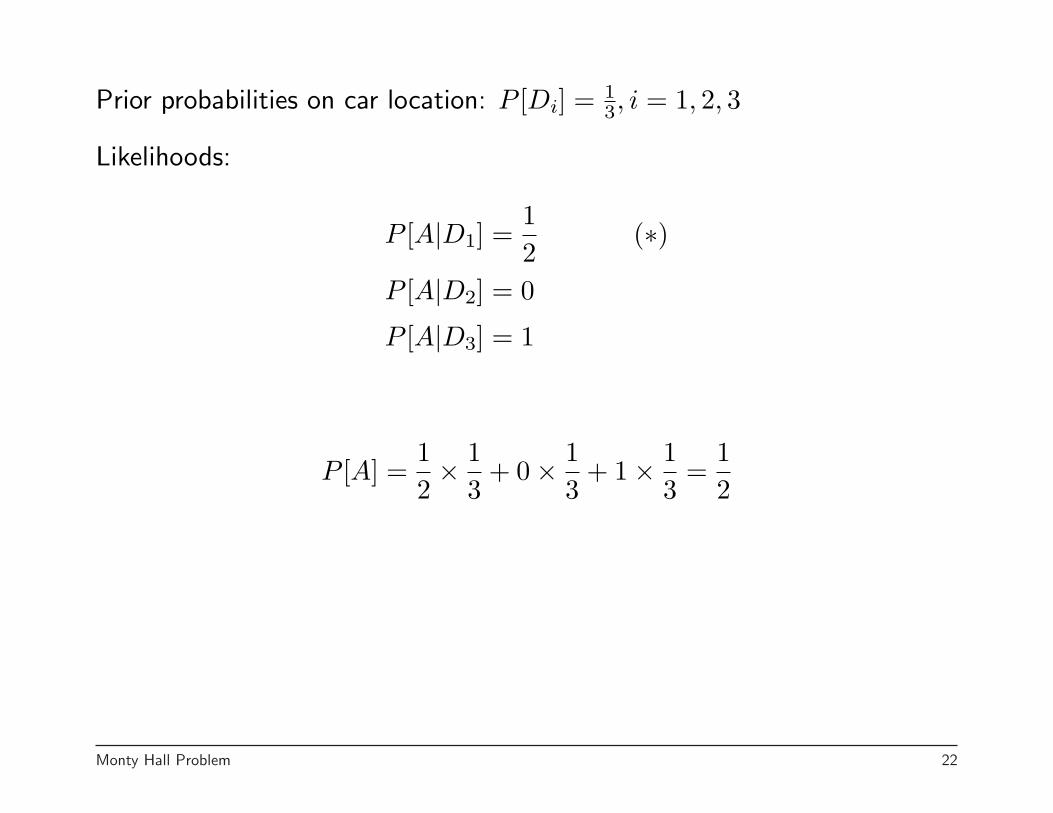
Prior probabilities on car location: P [Di] = 13, i = 1, 2, 3
Likelihoods:
P [A|D1] =12
(∗)P [A|D2] = 0
P [A|D3] = 1
P [A] =12× 1
3+ 0× 1
3+ 1× 1
3=
12
Monty Hall Problem 22

Posterior probabilities on car location:
P [D1|A] =12 × 1
312
=13
No change!
P [D2|A] =0× 1
312
= 0
P [D3|A] =1× 1
312
=23
Bigger!
If you are willing to assume that when two empty doors are available,Monty will randomly choose one of them to open (with equal probability)(assumption *), then you should switch. You’ll win the car 2
3 of the time.
Monty Hall Problem 23
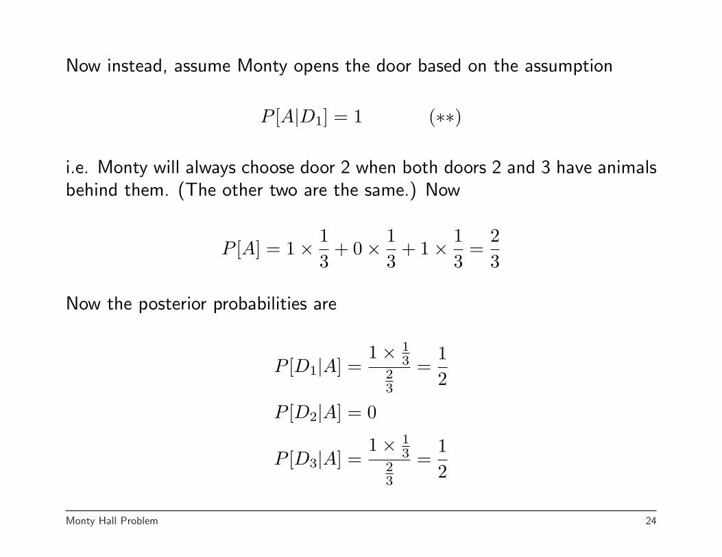
Now instead, assume Monty opens the door based on the assumption
P [A|D1] = 1 (∗∗)
i.e. Monty will always choose door 2 when both doors 2 and 3 have animalsbehind them. (The other two are the same.) Now
P [A] = 1× 13
+ 0× 13
+ 1× 13
=23
Now the posterior probabilities are
P [D1|A] =1× 1
323
=12
P [D2|A] = 0
P [D3|A] =1× 1
323
=12
Monty Hall Problem 24
So in this situation, switching doesn’t help (doesn’t hurt either).
Note: This is an extremely subtle problem that people have discussedfor years (go do a Google search on Monty Hall Problem). Some of thediscussion goes back before the show Let Make a Deal ever showed upon TV. The solution depends on precise statements about how doors arechosen to be opened. Changing the assumptions can lead to situationsthat changing can’t help and I believe there are situations where changingcan actually be worse. They can also lead to situations where the areadvantages to picking certain doors initially.
Monty Hall Problem 25

General Multiplication Rule
The multiplication rule discussed earlier can be extended to an arbitrarynumber of events as follows
P [A1 ∩A2 ∩ . . . ∩An] =
P [A1]× P [A2|A1]× P [A3|A1A2]× . . .× P [An|A1A2 . . . An−1]
This rule can be used to build complicated probability models.
General Multiplication Rule 26
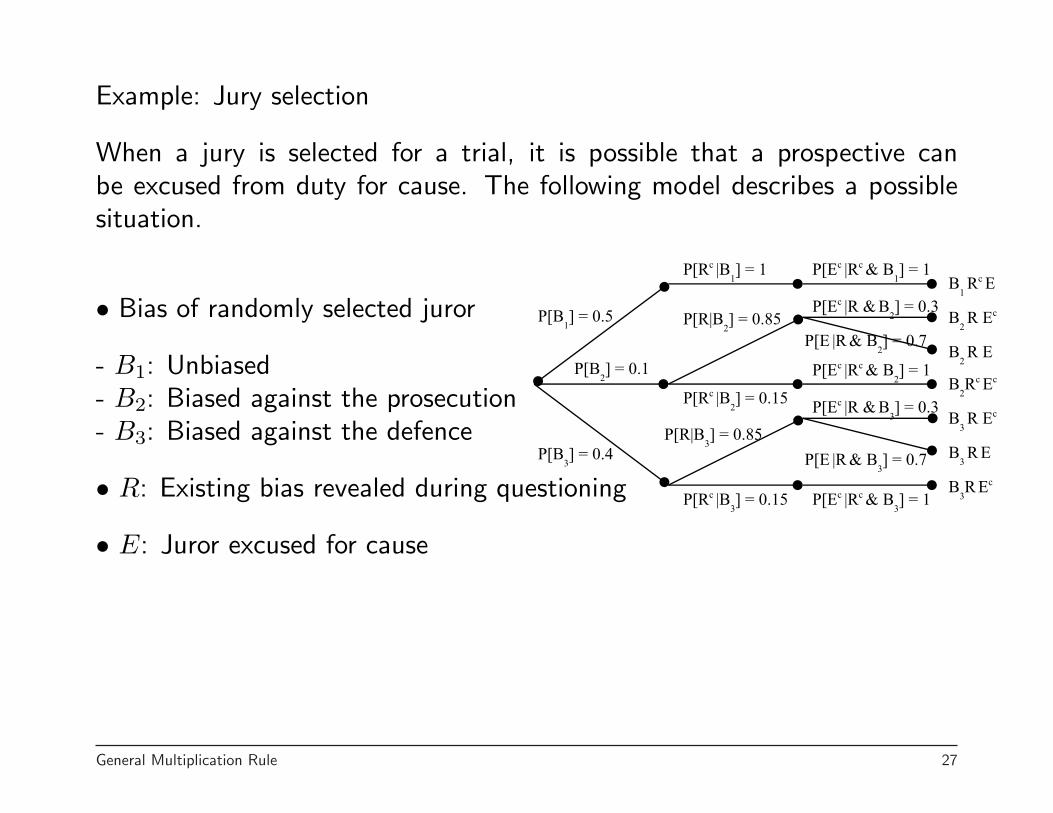
Example: Jury selection
When a jury is selected for a trial, it is possible that a prospective canbe excused from duty for cause. The following model describes a possiblesituation.
• Bias of randomly selected juror
- B1: Unbiased- B2: Biased against the prosecution- B3: Biased against the defence
• R: Existing bias revealed during questioning
• E: Juror excused for cause
General Multiplication Rule 27

The probability of any combination of these three factors can be determinedby multiplying the correct conditional probabilities. The probabilities for alltwelve possibilities are
R Rc
E Ec E Ec
B1 0 0 0 0.5000
B2 0.0595 0.0255 0 0.0150
B3 0.2380 0.1020 0 0.0600
For example P [B2 ∩R ∩ Ec] = 0.1× 0.85× 0.3 = 0.0255.
General Multiplication Rule 28

From this we can get the following probabilities
P [E] = 0.2975 P [Ec] = 0.7025P [R] = 0.4250 P [Rc] = 0.5750
P [B1 ∩ E] = 0 P [B2 ∩ E] = 0.0595 P [B3 ∩ E] = 0.238P [B1 ∩ Ec] = 0.5 P [B2 ∩ Ec] = 0.0405 P [B3 ∩ Ec] = 0.162
From these we can get the probabilities of bias status given that a personwas not excused for cause from the jury.
P [B1|Ec] = 0.50.7025 = 0.7117 P [B1|E] = 0
0.2975 = 0
P [B2|Ec] = 0.04050.7025 = 0.0641 P [B2|E] = 0.0595
0.2975 = 0.2
P [B3|Ec] = 0.16200.7025 = 0.2563 P [B3|E] = 0.238
0.2975 = 0.8
General Multiplication Rule 29