Joint Data Streaming and Sampling Techniques for Detection of Super Sourcesand Destinations

Qi (George) Zhao Abhishek Kumar Jun (Jim) XuCollege of Computing, Georgia Institute of Technology

Abstract

Detecting the sources or destinations that have communi-cated with a large number of distinct destinations or sourcesduring a small time interval is an important problem innetwork measurement and security. Previous detection ap-proaches are not able to deliver the desired accuracy at highlink speeds (10 to 40 Gbps). In this work, we propose twonovel algorithms that provide accurate and efficient solu-tions to this problem. Their designs are based on the in-sight that sampling and data streaming are often suitablefor capturing different and complementary regions of theinformation spectrum, and a close collaboration betweenthem is an excellent way to recover the complete informa-tion. Our first solution builds on the standard hash-basedflow sampling algorithm. Its main innovation is that thesampled traffic is further filtered by a data streaming mod-ule which allows for much higher sampling rate and hencemuch higher accuracy. Our second solution is more sophis-ticated but offers higher accuracy. It combines the powerof data streaming in efficiently estimating quantities asso-ciated with a given identity, and the power of sampling incollecting a list of candidate identities. The performanceof both solutions are evaluated using both mathematicalanalysis and trace-driven experiments on real-world Inter-net traffic.

1 IntroductionMeasurement of flow-level statistics, such as total activeflow count, sizes and identities of large flows, per-flowtraffic, and flow size distribution are essential for networkmanagement and security. Measuring such information onhigh-speed links (e.g., 10 Gbps) is challenging since thestandard method of maintaining per-flow state (e.g., us-ing a hash table) for tracking various flow statistics is pro-hibitively expensive. More specifically, at very high linkspeeds, updates to the per-flow state for each and every in-coming packet would be feasible only through the use ofvery fast and expensive memory (typically SRAM), whilethe size of such state is very large [7] and hence too expen-sive to be held in SRAM. Recently, the techniques for ap-proximately measuring such statistics using a much smallerstate, based on a general methodology called network datastreaming, have been used to solve some of the aforemen-tioned problems [5, 6, 12, 11, 22]. The main idea in net-

work data streaming is to use a small and fast memory toprocess each and every incoming packet in real-time. Sinceit is impractical to store all information in this small mem-ory, the principle of data streaming is to maintain only theinformation most pertinent to the statistic to be measured.In this work, we design data streaming algorithms thathelp detect super sources and destinations. A super source1is a source that has a large fan-out (e.g., larger than a pre-defined threshold) defined as the number of distinct des-tinations it communicates with during a small time in-terval. The concepts of super destination and fan-in canbe defined symmetrically. Our schemes in fact solve astrictly harder problem than making a binary decision ofwhether a source/destination is a super source/destinationor not: They actually provide accurate estimates of the fan-outs/fan-ins of potential super sources/destinations. In thiswork a source can be any combination of “source” fieldsfrom a packet header such as source IP address, source portnumber, or their combination, depending on target applica-tions. Similarly, a destination can be any combination ofthe “destination” fields from a packet header. We refer tothe source-destination pair of a packet as the flow label anduse these two terms interchangeably in the rest of this pa-per.The problem of detecting super sources and destinationsarises in many applications of network monitoring and se-curity. For example, port-scans probe for the existence ofvulnerable services across the Internet by trying to connectto many different pairs of destination IP address and portnumber. This is clearly a type of super source under ourdefinition. Similarly, in a DDoS (Distributed Denial of Ser-vice) attack, a large number of zombie hosts flood packetsto a destination. Thus the problem of detecting the launchof DDoS attacks can be viewed as detecting a super desti-nation. This problem also arises in detecting worm prop-agation and estimating their spreading rates. An infectedhost often propagates the worm to a large number of des-tinations, and can be viewed as a super source. Knowingits fan-out allows us to estimate the rate at which the wormmay spread. Another possible instance lies in peer-to-peerand content distribution networks, where a few servers orpeers might attract a larger number of requests (for con-tent) than they can handle while most of others in the net-work are relatively idle. Being able to detect such “hotspots” (a type of super destination) in real-time helps bal-

Internet Measurement Conference 2005 USENIX Association 77

ance the workload and improve the overall performance ofthe network. A number of other variations of the above ap-plications, such as detecting flash crowds [9] and reflectorattacks [15], also motivate this problem.Techniques proposed in the literature for solving thisproblem typically maintain per-flow state, and cannot scaleto high link speeds of 10 or 40 Gbps. For example, todetect port-scans, the widely deployed Intrusion Detec-tion System (IDS) Snort [19] maintains a hash table ofthe distinct source-destination pairs to count the destina-tions each source talks to. A similar technique is usedin FlowScan [17] for detecting DDoS attacks. The inef-ficiency in such an approach stems from the fact that mostof the source-destination pairs are not a part of port scansor DDoS attacks. Yet, they result in a large number ofsource-destination pairs that can be accommodated onlyin DRAM, which cannot support the high access rates re-quired for updates at line speed. More recent work [20] hasoffered solutions based on hash-based flow sampling tech-nique. However, its accuracy is limited due to the typicallylow sampling rate imposed by some inherent limitations ofthe hash-based flow sampling technique discussed later inSection 3. A more comprehensive survey of related workis provided in Section 7.In this paper we propose two efficient and accurate datastreaming algorithms for detecting the set of super sourcesby estimating the fan-outs of the collected sources. Thesealgorithms can be easily adapted symmetrically for detect-ing the super destinations. Their designs are based on theinsight that (flow) sampling and data streaming are oftensuitable for capturing different and complementary regionsof the information spectrum, and a close collaboration be-tween them is an excellent way to recover the complete in-formation. This insight leads to two novel methodologiesof combing the power of streaming and sampling, namely,“filtering after sampling” and “separation of counting andidentity gathering”. Our two solutions are built upon thesetwo methodologies respectively.Our first solution, referred to as the simple scheme, isbased on the methodology of “filtering after sampling”. Itenhances the traditional hash-based flow sampling algo-rithm to approximately count the fan-outs of the sampledsources. As suggested by its name, the design of this solu-tion is very simple. Its main innovation is that the sampledtraffic is further filtered by a simple data streaming module(a bit array), which guarantees that at most one packet fromeach flow is processed. This allows for much higher sam-pling rate (hence much higher accuracy) than achievablewith traditional hash-based flow sampling. Our second so-lution, referred to as the advanced scheme, is more sophis-ticated than the simple scheme but offers even higher accu-racy. Its design is based on the methodology of “separationof counting and identity gathering”, which combines thepower of streaming in efficiently estimating quantities (e.g.,

fan-out) associated with a given identity, and the power ofsampling in generating a list of candidate identities (e.g.,sources). Through rigorous theoretical analysis and exten-sive trace-driven experiments on real-world Internet traffic,we demonstrate these two algorithms produce very accu-rate fan-out estimations.We also extend our advanced scheme for detecting thesources that have large outstanding fan-outs, defined as thenumber of distinct destinations it has contacted but hasnot obtained acknowledgments (TCP ACK) from. Thisextension has several important applications. One exam-ple is that in port-scans, the probing packets, which targeta large number of destinations, will receive acknowledg-ments from only a small percentage of them. Another ex-ample is distributed TCP SYN attacks. In this case, thevictim’s TCP acknowledgments (SYN/ACK packets) to alarge number of hosts for completing the TCP handshake(the second step) are not acknowledged. Our evaluationon bidirectional traffic collected simultaneously on a linkshows that our solution estimates outstanding fanout withhigh accuracy.The rest of this paper is organized as follows. In the nextsection, we present our design methodologies and providean overview of the proposed solutions. Sections 3 and 4 de-scribe the design of the two schemes in detail respectivelyand provide a theoretical analysis of their complexity andaccuracy. Section 5 presents an extension of our schemefor estimating outstanding fan-outs. We evaluate our solu-tions in Section 6 using packet header traces of real-worldInternet traffic. We discuss the related work in Section 7before concluding in Section 8.

2 Overview of our schemesAs we mentioned above, accurate measurement and mon-itoring in high speed networks are challenging becausethe traditional per-flow schemes cannot scale to high linkspeeds. As a stop-gap solution, packet sampling has beenused to keep up with high link speeds. In packet sampling,a small fraction p of traffic is sampled and processed. Sincethe sampled packets constitute a much lower volume thanthe original traffic, a per-flow table stored in relatively in-expensive DRAM can handle all the updates triggered bythe sampled packets in real-time [14]. Thus we can typi-cally obtain complete information contained in the sampledtraffic. The statistics of the original traffic are then inferredfrom that of the sampled traffic by “inverting” the samplingprocess, i.e., by compensating for the effects of sampling.However the accuracy of such sampling-based estimationsis usually low, because the error is scaled by 1/p and p istypically small (e.g., 1/500) to make the sampling opera-tion computationally affordable [4, 11, 8]. In other words,although the sampling-based approach allows for 100% ac-curate digesting of information on sampled traffic, a largeamount of information may be lost during the sampling

Internet Measurement Conference 2005 USENIX Association78

process.Network data streaming2 has begun to be recognized asa better alternative to sampling for measurement and mon-itoring of high-speed links [10]. Contrary to sampling, anetwork data streaming algorithm will process each andevery packet passing through a high-speed link to glean themost important information for answering a specific typeof query, using a small yet well-organized data structure.This data structure is small enough to be fit into fast (yetexpensive) SRAM, allowing it to keep up with high linkspeeds. The challenge is to design this data structure insuch a way that it encodes the information we need, for an-swering the query, in a succinct manner. Data streamingalgorithms, if available, typically offer much more accu-rate estimations than sampling for measuring network flowstatistics. This is because, intuitively the sampling throwsaway a large percentage of information up front, while datastreaming, which processes each and every packet, is oftenable to retainmost of the most important information insidea small SRAM module.In our context of detecting super sources, however, bothsampling and data streaming are valuable for capturing dif-ferent and complementary regions of the information spec-trum, and a close collaboration between them is used torecover the complete information. There are two parts ofinformation that we would like to know in finding supersources: one is the identities (e.g., IP addresses) of thesources that may be super sources. The other is the fan-out associated with each source identity. We observe thatdata streaming algorithms can encode the fan-outs of var-ious sources into a very succinct data structure. Such adata structure, however, typically only provides a lookupinterface. In other words, if we obtain a source identitythrough other means, we are able to look up the data struc-ture to obtain its (approximate) fan-out, but the data struc-ture itself cannot produce any identities and is undecod-able without such identities being supplied externally. Onthe other hand, sampling is an excellent way of gatheringsource identities though it is not a great counting device aswe described earlier.The above observation leads to one of the two aforemen-tioned design methodologies, i.e., separating identity gath-ering and counting. The idea is to use a streaming datastructure as a counting device and use sampling to gatherthe identities of potential super sources. Then we look upthe streaming data structure using the gathered identities toobtain the corresponding counts. This methodology is usedin our advanced scheme that employs a 2-dimensional bitarray as the counting device, in parallel with an identitygathering module that adopts an enhanced form of sam-pling. We show that our sampling module has vanishinglysmall probability of missing the identity of any actual supersources and the estimation module produces highly accu-rate estimates of the fan-out of the potential super sources.

This scheme is especially suitable for very high link speedsof 10 Gbps and above. We describe this scheme in Sec-tion 4.We also explore another way of combing sampling andstreaming, i.e., “filtering after sampling”. Its idea is to em-ploy a data streaming module between the sampling op-eration and the final processing procedure to efficiently en-code whether a flow has been seen before. A careful designof this module guarantees that at most one packet in eachflow needs to be processed. This allows us to achieve muchhigher sampling rate and hence much higher accuracy thanthe traditional flow sampling scheme. This solution worksvery well for relatively lower link speeds (e.g., 10 Gbps andbelow). We describe this scheme in detail in Section 3.

3 The simple schemeIn this section we present a relatively simple scheme fordetecting super sources. It builds upon the traditional hash-based flow sampling technique but can achieve a muchhigher sampling rate, and hence more accurate estimation.We begin with a discussion of some limitations of the tradi-tional hash-based sampling approach, and then describe oursolution that alleviates these limitations. We also present ananalysis of the complexity and accuracy of the scheme.

3.1 Limitations of traditional hash-basedflow sampling

There are two generic sampling approaches for networkmeasurement: packet sampling and flow sampling. In theformer approach, each packet is sampled independentlywith a certain probability, while in the latter, the samplingdecision is made at the granularity of flows (i.e., all packetsbelonging to sampled flows are sampled). In the following,we only consider flow sampling since packet sampling isnot suitable for our context of detecting super sources. 3

A traditional flow sampling algorithm that estimates thefan-outs of sources works as follows. The algorithm ran-domly samples a certain percentage (say p) of source-destination pairs using a hashing technique (describednext). The fan-out of each source in the sampled pairs iscounted and then scaled by 1/p to obtain an estimate ofthe fan-out of the source in the original traffic (i.e., beforesampling). This counting process is typically performedusing a hash table that stores the fan-out values (after sam-pling) of all sources seen in the sampled traffic so far, anda newly sampled flow will increment the fan-out counterof the corresponding hash node (or trigger the creation of anew node). Since the estimation error is also scaled by 1/p,it is desirable to make the sampling rate p as high as pos-sible. However, we will show that, at high link speeds, thetraditional hash-based flow sampling approachmay preventus from achieving high sampling rate needed for accurateestimation.

Internet Measurement Conference 2005 USENIX Association 79

Flow sampling is commonly implemented using a sim-ple hashing technique [3] as follows. First a hash functiong that maps a flow label to a value uniformly distributedin [0, 1) is fixed. When a packet arrives, its flow label ishashed by g. Given a sampling probability p, the flow issampled if and only if the hashing result is no more thanp. Recall that the purpose of flow sampling is to reducethe amount of traffic that needs to be processed by theaforementioned hash table which performs the counting.Clearly, it is desirable that a hash table that runs slightlyfaster than p times the link speed, can keep up with the in-coming rate of the sampled traffic (with rate p). For exam-ple, we would like a hash table (in DRAM) that is able toprocess a packet in 400ns to handle all traffic sampled froma link with 10 million packets per second (i.e., one packetarrival per 100ns on the average) with slightly less than25% sampling rate. Unfortunately, we cannot achieve thisgoal with the current hash-based flow sampling approachfor the following reason.With hash-based flow sampling, if a flow is sampled, allpackets belonging to the flow need to be processed by thehash table. Internet traffic is very bursty in the sense thatthe packets belonging to a flow tend to arrive in bursts anddo not interleave well with packets from other flows andis also known to exhibit the following characteristic [5]: asmall number of elephant flows contain most of the overalltraffic while the vast majority of the flows are small. If afew elephant flows are sampled, their packets could gen-erate a long burst of sampled traffic that has much higherrate than that can be handled by the hash table4. Therefore,with hash-based flow sampling, the sampling rate p has tobe much smaller than the ratio between the operating speedof the hash table and the arrival rate of traffic, thus lead-ing to large estimation errors as discussed before. In thefollowing subsection, we present an efficient yet simple so-lution to this problem, allowing the sampling rate to reachor even well exceed this ratio.In [20] the authors propose a one-level filtering algo-rithm which uses the hash-based flow sampling approachdescribed above, in conjunction with a hash table for count-ing the fan-out values. It does not specify whether DRAMor SRAM will be used to implement the hash table. IfDRAM were used, it will not be able to achieve a highsampling rate as discussed before. If SRAM were used, thememory cost is expected to be prohibitive when the sam-pling rate is high. This algorithm appears to be effectiveand accurate for monitoring lower link speeds, but cannotdeliver a high estimation accuracy when operating at highlink speeds such as 10Gbps (the target link speeds are notmentioned in [20]).

3.2 Our schemeWe design a filtering technique that completely solves theaforementioned problem. It allows the sampling rate to be

Pakcet Stream

samplingflow

Traditional flow sampling:

Filtering after sampling:

Pakcet Stream

samplingflow Hash Estimation Result

Data

module

streamingHash Estimation Result

Table

Table

Figure 1: Traditional flow sampling vs. filtering after sampling

1. Initialize2. G[r] := 0, r=1,2,. . . , w3. /* w is the size of the array */4. u := w

5. /* variable u keep track the number of “0”s in G */

6. Filtering after sampling7. Upon each incoming sampled packet pkt

8. r := h(< pkt.src, pkt.dst >)9. if G[r] = 010. s := pkt.src

11. cNs := cNs + w

u

12. /* The (s, cNs) pairs are maintained as a hashtable L. */

13. G[r] := 114. u := u − 115. /* The number of “0”s is decreased by 1 */

Figure 2: Algorithm of updating data streaming module.

very close to the ratio between the hash table speed andthe link speed in the worst-case and well exceed the ra-tio otherwise. Its conceptual design is shown in Figure 1.Compared with the traditional flow sampling approach, ourapproach places a data streamingmodule between the hash-based flow sampling module and the hash table (for count-ing). This streaming module guarantees that at most onepacket from each sampled flow needs to be processed bythe hash table. This will completely smooth out the afore-mentioned traffic bursts in the flow-sampled traffic, sincesuch bursts are caused by highly bursty arrivals from oneor a small number of elephant flows and now only the firstpackets of these flowsmay trigger updates to the hash table.The data structure and algorithm of the data streamingmodule are shown in Figure 2. Its basic idea is to use abit array G to remember whether a flow label, a source-destination pair in our context, has been processed by thehash table. Let the size of the array be w bits. We fix ahash function h that maps a flow label to a value uniformlydistributed in [1, w]. The array is initialized to all “0”s atthe beginning of a measurement epoch. Upon the arrival ofa packet pkt, we hash its flow label (< pkt.src, pkt.dst >)using h and the result r is treated as an index into the array

Internet Measurement Conference 2005 USENIX Association80

G. If G[r] is equal to 1, our algorithm concludes that apacket with this flow label has been processed earlier, andtakes no further action. Otherwise (i.e.,G[r] is 0), this flowlabel will be processed to update the corresponding counterNpkt.src maintained in a hash table L. ThenG[r] is set to 1to remember the fact that a packet with this flow has beenseen and processed. This method clearly ensures that atmost one packet from each sampled flow is processed by L.However, due to hash collisions, some sampled flows maynot be processed at all since their corresponding bits in Gwould be set by their colliding counterparts.5 The updateprocedure of the hash table L, described next, statisticallycompensates for such collisions.Now we explain our statistical estimator, which is thecomputation result of the hash table update procedureshown in Figure 2 (line 11). Suppose the number of “0” en-tries in G (with size w) is u right before a packet pkt withsource s arrives (s := pkt.src in line 10). Assume pkt be-longs to a new flow and its flow label hashes to an index r.The value of G[r] has value 0 with probability u

w. There-

fore to obtain an unbiased estimator N̂s of the fan-out ofthe source s on the sampled traffic, we should statisticallycompensate for the fact that with probability 1− u

w, the bit

G[r] has value 1 and pkt will miss the update to L due toaforementioned hash collisions. It is intuitive that if we addwuto N̂s, the resulting estimator is unbiased. To be more

precise, suppose in a measurement epoch, the hash table isupdated by altogether K packets {pktj , j = 1, 2, ...,K}from a source s, whose flow labels hash to locations rj ’swhere G[rj ] = 0, and there are uj 0’s in G right beforepktj arrives, respectively. The output of the hash table L,which is an unbiased estimator of the fan-out of s on thesampled traffic, is

N̂s =K∑

j=1

w

uj

(1)

We show in the following lemma that this is an unbiasedestimator of Ns and its proof can be found in [24].

Lemma 1 N̂s is an unbiased estimator of Ns, i.e.,E[N̂s] = Ns.

Then an unbiased estimator of the fan-out Fs of source sis given by scaling N̂s by 1/p, i.e.,

F̂s =1

p

K∑

j=1

w

uj

(2)

where p is the sampling rate used in the flow sampling.We show in the following theorem that the estimator F̂s isunbiased. Its proof uses Lemma 1 and is also provided in[24].

Theorem 1 F̂s is an unbiased estimator of Fs, i.e.,E[F̂s] = Fs.

We now demonstrate that this solution will completelysmooth out the aforementioned problem of traffic bursts ,and allow the sampling rate to be close to the ratio betweenthe hash table speed and the link rate, the theoretical upperlimit in the worst case. The worst case for our scheme isthat each flow contains only one packet (e.g., in the case ofDDoS attacks)6. Even in this worst case, the update timesto the hash table (viewed as a random process) is very closeto Poisson7 (nonhomogeneous as the value of u varies overtime) since each new flow is sampled independently. Dueto the “benign” nature of this arrival process, by employinga tiny SRAM buffer (e.g., holding 20 flow labels of 64 ∼100 bits each), a hash table that operates slightly faster thanthe average rate of this process will only miss a negligiblefraction of updates due to buffer overflow. This processcan be faithfully modeled as a Markov chain for rigorousanalysis. We elaborate it with a numerical example in [24]and omit it here due to lack of space.Notice that in Figure 2 the variable u, the number of “0”entries in G, decreases as more and more sampled flowsare processed. When more and more packets pass throughthe data streaming module, u becomes small and hence theprobability for a new flow to be recorded, u

w, decreases.

Thereby the estimation error will increase. To maintainhigh accuracy, we specify a minimum value umin for u.Once the value of u drops below umin, the estimation pro-cedure will use a new array (set to all “0”s initially) andstart a new measurement epoch (with an empty hash ta-ble). Two sets of arrays and hash tables will be operated inan alternating manner so that the measurement can be per-formed without interruption. The parameter umin is typi-cally set to around w/2 (i.e., “half full”).

3.3 Complexity analysisThe above scheme has extremely low storage (SRAM)complexity and allows for very high streaming speed.Memory (SRAM) consumption. Each processed flowonly consumes a little more than one bit in SRAM. Thusa reasonable amount of SRAM can support very high linkspeeds. For example, assuming the average flow size of 10packets [11], 512KB SRAM is enough to support a mea-surement epoch which is slightly longer than 2 secondsfor a link with 10 million packets per second even withoutperforming any flow sampling. With 25% flow samplingwhich is typically set for OC-192 links the SRAM require-ment is even brought down to 128KB.8Streaming speed. Our algorithm in Figure 2 has twobranches to deal with the packets arriving at the datastreamingmodule. If the corresponding bit is “1”, the pack-ets only require one hash function computation and oneread to SRAM. Otherwise they require one hash functioncomputation, one read and one write (at the same location)to SRAM and an update to the hash table. Using efficienthardware implementation of hash function [18] and 5ns

Internet Measurement Conference 2005 USENIX Association 81

StreamingOnline

Module Module

1. Update 2. Sample

Packet stream

Identity

AlgorithmEstimation5. Estimation Result

Sampling

4. Query3. Data digest

Figure 3: System model of the advanced scheme

SRAM, all operations in the data streaming module can befinished in 10’s of ns in both cases.

3.4 Accuracy analysisNowwe establish the following theorem to characterize thevariance of the estimator F̂s in Formula 2. Its proof can befound in [24]

Theorem 2

V ar[F̂s] ≈

∑pFs

j=1w−uj

uj

p2+

Fs(1 − p)

p

Remark: The above variance consists of two terms. Thefirst term corresponds to the variance of the error term inestimating the sampled fan-out, scaled by 1

p2 (to compen-sate for sampling), and the second term corresponds to thevariance of the error term in inverting flow sampling pro-cess. Since these two errors are approximately orthogonalto each other, their total variance is the sum of their indi-vidual variances.

4 The advanced schemeIn this section we propose the advanced scheme that ismore sophisticated than the simple scheme but can offermore accurate fan-out estimations. It is based on the afore-mentioned design methodology of separating identity gath-ering from counting. Its system model is shown in Fig-ure 3. There are two parallel modules processing the in-coming packet stream. The data streaming module encodesthe fan-out information for each and every source (arc 1 inFigure 3) into a very compact data structure, and the iden-tity sampling module captures the candidate source identi-ties which have potential to be super sources (arc 2). Thesesource identities are then used by an estimation algorithmto look up the data structure (arc 3) produced by the datastreaming module (arc 4) to get their corresponding fan-outestimates. The design of these modules are described in thefollowing subsections.

4.1 Online streaming moduleThe data structure used in the online streaming module isquite simple: anm×n 2-dimensional bit arrayA. The bits

3 4 521 . . . n

...

1 1 1

11

11

1 1 1

1

11

1

1

23

54

m

1

1

1

1

1 1

111

11

11

111

11

1 1 1

src dst

h’

h hh 2 31

2D bit array A

00 0 0 0 0 0 0 0 00 0

00000

0 0 0 0 0 0 0 0 0 000

00000000000

000000 0 0 0 0 0 0 0 0

00000

000

00000

000

00 00

000 0

0

0 1

000

0

0000

0

0

Figure 4: An instance of online streaming module

1. Initialize2. A[i, j] := 0, i = 1, 2, ..., m j = 1, 2, · · · , n

3. Update4. Upon the arrival of a packet pkt

5. row := h′(< pkt.src, pkt.dst >)6. for i := 1 to k

7. col := hi(pkt.src)8. A[row, col] := 1

Figure 5: Algorithm of online streaming module

in A are set to all “0”s at the beginning of each measure-ment epoch. The algorithm of updating A is shown in Fig-ure 5. Upon the arrival of a packet pkt, pkt.src is hashed byk independent9 hash functions h1, h2, · · · , hk with range[1..n]. The hashing results h1(pkt.src), h2(pkt.src), ...,hk(pkt.src) are viewed as column indices into A. Inour scheme, k is set to 3, and the rationale behind itwill be discussed in Section 4.3. Then, the flow label< pkt.src, pkt.dst > is hashed by another independenthash function h′ (with range [1..m]) to generate a row in-dex of A. Finally, the k bits located at the intersectionsof the selected row and columns are set to “1”. An exam-ple is shown in Figure 4, in which the three intersectionbits (circled) are set to “1”s. When A is filled (by “1”)to a threshold percentage we terminate the current mea-surement epoch and start the decoding process10. In Sec-tion 4.2, we show that the above process produces a verycompact and accurate (statistical) encoding of the fan-outsof the sources, and present the corresponding decoding al-gorithm.Readers may feel that the above 2D bit arrayA is a vari-ant of Bloom filters [1]. This is not the case since althoughits encoding algorithm is similar to that of a Bloom filter(flipping some bits to “1”s), we decode the 2D bit arrayfor a different kind of information (the fan-out count) thanif we really use it as a Bloom filter (check if a particularsource-destination pair has appeared). Our encoding algo-

Internet Measurement Conference 2005 USENIX Association82

rithm is not well engineered for being used as a Bloom fil-ter. And our decoding algorithm, shown next, is also fun-damentally different from that of a Bloom filter.The proposed online streaming module has very lowmemory consumption and high streaming speed:Memory (SRAM) consumption. Our scheme is extremelymemory-efficient. Each source-destination pair (flow) willset 3 bits in the bit vectors to “1”s and consume a littlemore than 3 bits of SRAM storage11. We will show thatthe scheme provides very high accuracy using reasonableamount of SRAM (e.g., 128KB) in Section 6.Streaming speed. Each update requires only 4 hash func-tion computations and 3 writes to the SRAM. We requirethat these four hash functions are independent and amend-able to hardware implementation. They can be chosen fromthe H3 hash function family [2, 18], which, with hard-ware implementation, can produce a hash output within afew nanoseconds. Then with commodity 5ns SRAM ourscheme would allow around 40million packets per second,thereby supporting 40 Gbps traffic stream assuming a con-servative average packet size of 1,000 bits.

4.2 Estimation moduleFor each source identity recorded by the sampling mod-ule (described later), the estimation module decodes its ap-proximate fan-out from the 2D bit array A, the output ofthe data streaming module. In this section, we describe thisdecoding algorithm in detail.When we would like to know Fs, the fan-out of thesource s, s is hashed by the hash functions h1, · · · , hk,which are defined and used in the online streaming mod-ule, to obtain k column indices. Let Ai, i = 1, 2, · · · , k, bethe corresponding columns (viewed as bit vectors). In thefollowing, we derive, step by step, an accurate and almostunbiased estimator of Fs, as a function of Ai, i = 1, 2, · · · ,k.Let the set of packets hashed into column Ai during thecorrespondingmeasurement epoch be Ti and the number ofbits in Ai that are “0”s be UTi

. Note that the value UTiis

a part of our observation since we can obtain UTifrom Ai

through simple counting, although the notation itself con-tains Ti, the size of which we would like to estimate. Recallthe size of the column vector is m. A fairly accurate esti-mator of |Ti|, the number of packets of Ti, adapted from[21], is

DTi= m ln

m

UTi

(3)

Note that Fs, the fan-out of the source s, is equal to |T1∩T2 ∩ · · · ∩ Tk|, if during the measurement epoch, no othersources are hashed to the same k columnsA1, A2, · · · , Ak.Otherwise |T1 ∩ T2 ∩ · · · ∩ Tk| is the sum of the fan-outs of all (more than 1) the sources that are hashed intoA1, A2, · · · , Ak. We show in the next section, that the

probability with which the latter case happens is very smallwhen k = 3. We obtain the following estimator of Fs,which is in fact derived as an estimator for |T1 ∩T2 ∩ · · · ∩Tk|.

F̂s =∑

1≤i≤k

DTi−

∑

1≤i1<i2≤k

DTi1∪Ti2

+∑

1≤i1<i2<i3≤k

DTi1∪Ti2

∪Ti3

+ · · · + (−1)k−1DT1∪T2···∪Tk(4)

Here DTi∪···∪Tj, is defined as m ln m

UTi∪···∪Tj

, whereUTi∪···∪Tj

denotes the number of “0”s in the bit vectorBTi∪···∪Tj

which is the result of hashing the set of pack-ets Ti ∪ · · · ∪ Tj into a single empty bit vector. The bitvectorBTi∪···∪Tj

is computed as the bitwise-OR of Ai,. . . ,Aj . One can easily verify the correctness of this computa-tion with respect to the semantics of BTi∪···∪Tj

.We need to show that the RHS of Formula 4 is a fairlygood estimator of |T1 ∩ T2 ∩ · · · ∩ Tk|. Note that

|T1 ∩ T2 ∩ · · · ∩ Tk| =∑

1≤i≤k

Ti −∑

1≤i1<i2≤k

Ti1 ∪ Ti2

+∑

1≤i1<i2<i3≤k

Ti1 ∪ Ti2 ∪ Ti3

+ · · · + (−1)k−1T1 ∪ T2 · · · ∪ Tk (5)

by the principle of inclusion and exclusion. SinceDTi∪···∪Tj

is a fairly good estimator of |Ti ∪ · · · ∪ Tj | ac-cording to [21], we obtain the RHS of Formula 4 by replac-ing the terms |Ti ∪ · · · ∪ Tj | in Formula 5 by DTi∪···∪Tj

,1 ≤ i < j ≤ k. Note that it is not correct to di-rectly use the bitwise-AND of A1, A2, ..., Ak for estimat-ing |T1∩T2∩· · ·∩Tk| using Formula 3, because the bit vec-tor corresponding to the result of hashing the set of packetsT1∩T2∩ ...∩Tk into an empty bit vector, is not equivalentto the bitwise-AND of A1, ..., Ak.The estimator in Formula 4 generalizes the result in [21]which is developed for the special case k = 2. We willshow that our scheme only needs to use the special case ofk = 3, which is

F̂s =DT1+ DT2

+ DT3− DT1∪T2

− DT1∪T3− DT2∪T3

+ DT1∪T2∪T3(6)

The computational complexity of estimating the fan-outof a source is dominated by 2k − k − 1 bitwise-OR op-erations among k column vectors. Such vectors can beencoded as one or more unsigned integers so that the bit-parallelism can significantly reduce the execution time.Since m is typically 64 bits in our scheme, the whole vec-tor can be held in two 32-bit integers. Therefore, in ourscheme where k = 3, estimation of the fan-out of each

Internet Measurement Conference 2005 USENIX Association 83

source only needs 8 bitwise-OR operations between 32-bitintegers. We also need to count the number of “0”s in avector (to get UT values). This can be sped up significantlyby using a pre-computed table (in SRAM) of size 262,144(= 216 × 4) bits that stores the number of “0”s in all 16-bitnumbers. Our estimation of the execution time shows thatour scheme is fast enough to support OC-768 operations.

4.3 Accuracy analysis

In this section we first briefly explain the rationale behindsetting k to 3 in the estimator and then analyze the accuracyof our estimator rigorously. We set k (the number of “col-umn” hash functions) to 3 due to the following two consid-erations. First, we mentioned before that if two sources s1

and s2 both are hashed to the same k columns, our decod-ing algorithm will give us an estimate of their total fan-out,when we use s1 or s2 to lookup the 2D array. We cer-tainly would like the probability with which this scenariooccurs to be as small as possible. This can be achievedby making k as large as possible. However, larger k im-plies larger computational and storage complexities at theonline streaming module. We will show that k = 3 makesthe probability of the aforementioned hash collision verysmall, and at the same time keeps the computational andstorage complexities of our scheme modest.

Nowwe derive η, the probability that at least two sourceshappen to hash to the same set of k columns by h1, h2, ...,hk. It is not hard to show, using straightforward combi-

natorial arguments, that η = 1 −(nk

S )S!

nkS , where S is thetotal number of the distinct sources during the measure-ment epoch. We observe that, given typical values for nand S, η is quite large when k = 2, but drops to a verylow value when k = 3. For example, when n = 16K andS = 100, 000, η is close to 1 when k = 2, but drops to0.002 when k = 3.

The following theorem characterizes the variance of theestimator in Formula 6, which is also its approximate meansquare error (MSE), since the estimator is almost unbiasedand the impact of η (discussed above) on the estimationerror is very small when k = 3. Its proof can be found in[24]. This is an extension of our previous variance analysisin [23] which is derived for the special case k = 2. Let tT

denote |T |/m, which is the load factor of the bit vector(ofsizem) when the corresponding set T of source-destinationpairs are hashed into it, in the following theorem.

0

0.01

0.02

0.03

0.04

0.05

0.06

20 30 40 50 60 70 80

PMF

Estimation

Actual Value-->

-σ--> <--σ

<--2σ-2σ-->

Figure 6: Distribution of the estimation from Monte-Carlo simu-lation (m = 64b, k = 3 and Fs = 50). σ is the standard deviationcomputed from Theorem 3

Theorem 3 The variance of F̂s is given by

V ar[F̂s] ≈ −m

3∑

i=1

f(tTi) − m

∑

1≤i1<i2≤3

f(tTi1∪Ti2

)

+ 2m(f(tT1∪(T2∩T3)) + f(tT2∪(T1∩T3)) + f(tT3∪(T2∩T1)))

+ 2m∑

1≤i1<i2≤3

f(tTi1∩Ti2

)

− 2m(f(tT1∩(T2∪T3)) + f(tT2∩(T1∪T3)) + f(tT3∩(T2∪T1)))

+ mf(tT1∪T2∪T3)

where f(t) = et − t − 1.

An example distribution of F̂s with respect to the actualvalueFs is shown in Figure 6. We obtained this distributionwith 20,000 runs of the Monte-Carlo simulations with thefollowing parameters. In this empirical distribution, the ac-tual fan-out Fs is 50, the size of the column vectorm is 64bits. The load factor is set to tTi

= 1.5 for 1 ≤ i ≤ 3. Also,since the sets T1, T2, and T3 have 50 flows in common, weset tTi∩Tj

= 5064 = 0.78125, for 1 ≤ i < j ≤ 3. Here we

implicitly assume that pairs of them do not have any flowsin common other than these 50 flows, which happens withvery high probability (= 1− 1

n2 + 1n3 ) anyway given a large

n (e.g., 16K). In this example the standard deviation σ isaround 6.4 as computed from Theorem 3. We observe thatthe size of the tail that falls outside 2 standard deviationsfrom the mean is very small (< 4%). This shows that, withhigh probability, our estimator will not deviate too muchfrom the actual value. In Section 6, the trace-driven experi-ments on the real-world Internet traffic will further validatethis.12Note that given the size ofm, our scheme is only able toaccurately estimate fan-out values up to m lnm + O(m),because if the actual fan-out Fs is much larger than that, wewill see all 1’s in the corresponding column vectors withhigh probability (due to the result of the “coupon collec-tor’s problem” [13]). In this case, the only information wecan obtain aboutFs is that it is no smaller thanm lnm. For-tunately, for the purpose of detecting super sources, this in-formation is good enough for us to declare s a super source,

Internet Measurement Conference 2005 USENIX Association84

as long as the threshold for super sources is much smallerthanm lnm. However, in some applications (e.g., estimat-ing the spreading speed of a worm), we may also want toknow the approximate fan-out value. This can be achievedusing amulti-resolution extension of our advanced scheme.The methodology of multi-resolution is quite standard andhas been used in several recent works [6, 12, 11]. The ex-tension in our context is straightforward. We omit its de-tailed specifications here in interest of space.

4.4 Identity sampling moduleThe purpose of this module is to capture the identities ofpotential super sources that will be used to look up the2D array to get their fan-out estimations. The filtering af-ter sampling technique proposed in Section 3 is adoptedhere with a slightly different recording strategy. Instead ofconstructing a hash table to record the sources and theirfan-out estimation, here we only record the source identi-ties sequentially in the DRAM. Since this strategy avoidsexpensive hash table operations and sequential writes toDRAM can be made very fast (using burst mode), veryhigh sampling rate can be achieved. With commodity 5nsSRAM and 60ns DRAM, this recording strategy will beable to process more than 12.5 million packets per second.At this speed, we can record 100% and 25% flow labelsfor OC-192 and OC-768 links respectively. With such ahigh sampling rate, the probability that the identity of areal super source misses sampling is very low. For exam-ple, given 25% sampling rate the probability that a sourcewith fan-out 50 fails to be recorded is only 5.6 × 10−7

(=(1 − 25%)50).

5 Estimating outstanding fan-outsIn this section we describe how to extend the advancedscheme to detect the sources that have contacted but havenot obtained acknowledgments from a large number of dis-tinct destinations (i.e., the sources with large outstandingfan-outs). Although both of our schemes have the potentialto support this extension we focus on the advanced schemein this work and leave the extension of the simple schemefor future research. In the following sections we show howto slightly modify the operations of the online streamingmodule and the estimation module of the advanced schemefor estimating outstanding fan-outs. The sampling moduledoes not need to be modified.

5.1 Online streaming moduleThe online streaming module employs two 2D bit arraysAand B of identical size and shape. The array A encodesthe fan-outs of sources in traffic in one direction (called“outbound”) in the same way as in the advanced scheme(shown in Figure 5). The array B encodes the fan-insof the destinations of the acknowledgment packets in theopposite direction (called “inbound”). Its encoding algo-

1. Initialize2. B[i, j] := 0, i = 1, 2, ..., m j = 1, 2, · · · , n

3. Update4. Upon the arrival of a packet pkt

5. if pkt is an acknowledgment packet6. row := h′(< pkt.dst, pkt.src >)7. for i := 1 to k

8. col := hi(pkt.dst)9. B[row, col] := 1

Figure 7: Algorithm for updating the 2D bit array B to recordACK packets

rithm is shown in Figure 7. It is a transposed version ofthe algorithm shown in Figure 5 in the sense that all oc-currences of “pkt.src” are replaced with with “pkt.dst”and “pkt.dst” with “pkt.src”. This transposition is neededsince a source in the outbound traffic appears in the in-bound acknowledgment traffic as a destination, and aftertransposing two packets that belong to a flow and its “ac-knowledgment flow” respectively will result in a write of“1” to the same bit locations in A and B respectively. Thisallows us to essentially take a “difference” between A andB to obtain the decoding of outstanding fan-outs of varioussources, shown next.

5.2 Estimation moduleWe compute the bitwise-OR ofA andB, denoted asA∨B.For each source s, we decode its fan-out from A∨B usingthe same decoding algorithm as described in Section 4.2.Similarly, we decode its fan-in in the acknowledgment traf-fic fromB. Our estimator of the outstanding fan-out of s issimply the former subtracted by the latter.Now we explain why this estimator will provide an accu-rate estimate of the outstanding fan-out of a source s. LetS1 be the set of flows whose source is “s” in the outboundtraffic. Let S2 be the set of flows whose destination is “s”in the inbound acknowledgment traffic. Clearly the quan-tity we would like to estimate is simply |S1 − S2|. Thecorrectness of our estimator is evident from the followingthree facts: (a) |S1 − S2| is equal to |S1

⋃S2| − |S2|; (b)

decoding from A ∨ B will result in a fairly accurate esti-mate of |S1

⋃S2| and (c) decoding from B will result in a

fairly accurate estimate of |S2|.

6 EvaluationIn this section, we evaluate the proposed schemes usingreal-world Internet traffic traces. Our experiments aregrouped into three parts corresponding to the three algo-rithms presented: the simple scheme, the advanced scheme,and its extension to estimate outstanding fan-outs. The ex-perimental results show that our schemes allow for accu-

Internet Measurement Conference 2005 USENIX Association 85

Trace # of sources # of flows # of packetsIPKS+ 119,444 151,260 1,459,394IPKS− 96,330 125,126 1,655,992USC 84,880 106,626 1,500,000UNC 55,111 101,398 1,495,701

Table 1: Traces used in our evaluation. Note that source is <

src IP, src port >, destination is dst IP and flow label is thedistinct source-destination pair.

rate estimation of fan-outs and hence the precise detectionof super sources.

6.1 Traffic Traces and Flow definitionsTrying to make the experimental data as representative aspossible, we use packet header traces gathered at three dif-ferent locations of the Internet, namely, University of NorthCarolina (UNC), University of Southern California (USC),and NLANR. The trace form UNC was collected on a 1Gbps access link connecting the campus to the rest of theInternet, on Thursday, April 24, 2003 at 11:00 am. Thetrace from USC was collected at their Los Nettos tracingfacility on Feb. 2, 2004. We also use a pair of unidirec-tional traces from NLANR: IPKS+ and IPKS−, col-lected simultaneously on both directions of an OC192c linkon June 1, 2004. The link connects Indianapolis (IPLS) toKansas City (KSCY) using Packet-over-SONET. This pairof traces is especially valuable to evaluate the extended ad-vanced scheme for estimating outstanding fan-outs. Allthe above traces are either publicly available or availablefor research purposes upon request. Table 1 summarizesall the traces used in the evaluation. We will use USC,UNC and IPKS+ to evaluate our simple scheme and ad-vanced scheme and use the concurrent traces IPKS+ andIPKS− to evaluate the extension.As mentioned before, a source/destination label can beany combination of source/destination fields from the IPheader. Two different definitions of source and destinationlabels are used in our experiments, targeting different ap-plications. In the first definition, source label is the tuple<src IP, src port> and destination label is <dst IP>. Thisdefinition targets applications such as detecting worm prop-agation and locating popular web servers. The flow statis-tics displayed in Table 1 use this definition. In the seconddefinition, Second, source label is <src IP> and destina-tion label is the tuple <dst IP, dst port>. This definitiontargets applications such as detecting infected sources thatconduct port scans. The experimental results presented inthis section use the first definition of source and destinationlabels unless noted otherwise.

6.2 Accuracy of the simple schemeIn this section, we evaluate the accuracy of the simplescheme in estimating the fan-outs of sources and in detect-

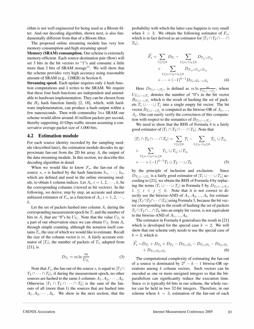
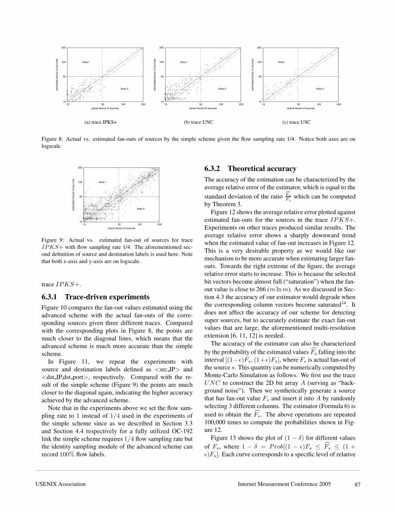
ing super sources. Figure 8 compares the fan-outs of thesources estimated using our simple scheme with the theiractual fan-outs in traces IPKS+, UNC, and USC re-spectively. In these experiments, a flow sampling rate of1/4 and a bit array of size 128K bits is used. The fig-ure only plots the points whose actual fan-out values areabove 15 since lower values (i.e., < 15) are not interestingfor finding super sources. The solid diagonal line in eachfigure denotes perfect estimation, while the dashed linesdenote an estimation error of ±15%. The dashed lines areparallel to the diagonal line since both x-axis and y-axis areon the log scale. Clearly the closer the points cluster aroundthe diagonal, the more accurate the estimation is. We ob-serve that the simple scheme achieves reasonable accuracyfor relatively large fan-outs in all three traces. Figure 8also reflects the false positives and negatives in detectingsuper sources. For a given threshold 50, the points that fallin “Area I” corresponds to false positives, i.e., the sourceswhose actual fan-outs are less than the threshold but theestimated fan-outs are larger than the threshold. Similarly,the points that fall in “Area II” corresponds to false nega-tives, i.e., the sources whose actual fan-outs are larger thanthe threshold but the estimated fan-outs are smaller thanthe threshold. We observe that in Figure 8, points rarelyfall into Areas I and II (i.e., very few false positives andnegatives13).While this scheme works well with 1/4 sampling rate,it cannot produce good estimations with smaller samplingrates (e.g., 1/16. We omit the experimental results heredue to lack of space.). However such lower sampling ratesmight be necessary to keep up with very high link speedssuch as 40 Gbps (OC-768).We repeat the above experiment under the aforemen-tioned second definition of source and destination, inwhich the source label is <src IP> and destination labelis <dst IP, dst port>. Figure 9 plots the estimated fan-outsof sources in trace IPKS+. With this definition the traceIPKS+ has 9,359 sources and 140,140 distinct source-destination pairs. We can see from the figure that our esti-mation is also quite accurate with this second definition ofsource and destination.

6.3 Accuracy of the advanced schemeIn this section we evaluate the accuracy of the advancedscheme using both trace-driven simulation and theoreticalanalysis. The estimation accuracy of the advanced schemeis a function of the various design parameters, includingthe size and shape of the 2D bit arrayA (i.e., the number ofrows m and columns n) and the number of hash functions(k).In the experiments we set the size of A to 128KB (64rows × 16,384 columns), k = 3 and the flow samplingrate to 1. This configuration is very space-efficient. Forexample it only uses 7 bits per flow on the average for the

Internet Measurement Conference 2005 USENIX Association86

15

50

100

200

15 50 100 200

estim

ated

fano

utof

sour

ces

actual fanout of sources

Area I

Area II

(a) trace IPKS+

15

50

100

200

15 50 100 200

estim

ated

fano

utof

sour

ces

actual fanout of sources

Area I

Area II

(b) trace UNC

15

50

100

200

15 50 100 200

estim

ated

fano

utof

sour

ces

actual fanout of sources

Area I

Area II

(c) trace USC

Figure 8: Actual vs. estimated fan-outs of sources by the simple scheme given the flow sampling rate 1/4. Notice both axes are onlogscale.

15

50

100

200

15 50 100 200

estim

ated

fano

utof

sour

ces

actual fanout of sources

Area I

Area II

Figure 9: Actual vs. estimated fan-out of sources for traceIPKS+ with flow sampling rate 1/4. The aforementioned sec-ond definition of source and destination labels is used here. Notethat both x-axis and y-axis are on logscale.

trace IPKS+.

6.3.1 Trace-driven experimentsFigure 10 compares the fan-out values estimated using theadvanced scheme with the actual fan-outs of the corre-sponding sources given three different traces. Comparedwith the corresponding plots in Figure 8, the points aremuch closer to the diagonal lines, which means that theadvanced scheme is much more accurate than the simplescheme.In Figure 11, we repeat the experiments withsource and destination labels defined as <src IP> and<dst IP,dst port>, respectively. Compared with the re-sult of the simple scheme (Figure 9) the points are muchcloser to the diagonal again, indicating the higher accuracyachieved by the advanced scheme.Note that in the experiments above we set the flow sam-pling rate to 1 instead of 1/4 used in the experiments ofthe simple scheme since as we described in Section 3.3and Section 4.4 respectively for a fully utilized OC-192link the simple scheme requires 1/4 flow sampling rate butthe identity sampling module of the advanced scheme canrecord 100% flow labels.

6.3.2 Theoretical accuracyThe accuracy of the estimation can be characterized by theaverage relative error of the estimator, which is equal to thestandard deviation of the ratio cFs

Fswhich can be computed

by Theorem 3.Figure 12 shows the average relative error plotted againstestimated fan-outs for the sources in the trace IPKS+.Experiments on other traces produced similar results. Theaverage relative error shows a sharply downward trendwhen the estimated value of fan-out increases in Figure 12.This is a very desirable property as we would like ourmechanism to be more accurate when estimating larger fan-outs. Towards the right extreme of the figure, the averagerelative error starts to increase. This is because the selectedbit vectors become almost full (“saturation”) when the fan-out value is close to 266 (m lnm). As we discussed in Sec-tion 4.3 the accuracy of our estimator would degrade whenthe corresponding column vectors become saturated14. Itdoes not affect the accuracy of our scheme for detectingsuper sources, but to accurately estimate the exact fan-outvalues that are large, the aforementioned multi-resolutionextension [6, 11, 12] is needed.The accuracy of the estimator can also be characterizedby the probability of the estimated values F̂s falling into theinterval [(1−ε)Fs, (1+ε)Fs], whereFs is actual fan-out ofthe source s. This quantity can be numerically computed byMonte-Carlo Simulation as follows. We first use the traceUNC to construct the 2D bit array A (serving as “back-ground noise”). Then we synthetically generate a sourcethat has fan-out value Fs and insert it into A by randomlyselecting 3 different columns. The estimator (Formula 6) isused to obtain the F̂s. The above operations are repeated100,000 times to compute the probabilities shown in Fig-ure 12.Figure 13 shows the plot of (1 − δ) for different valuesof Fs, where 1 − δ = Prob[(1 − ε)Fs ≤ F̂s ≤ (1 +ε)Fs]. Each curve corresponds to a specific level of relative

Internet Measurement Conference 2005 USENIX Association 87

15

50

100

200

15 50 100 200

estim

ated

fano

utof

sour

ces

actual fanout of sources

Area I

Area II

(a) trace IPKS+

15

50

100

200

15 50 100 200

estim

ated

fano

utof

sour

ces

actual fanout of sources

Area I

Area II

(b) trace UNC

15

50

100

200

15 50 100 200

estim

ated

fano

utof

sour

ces

actual fanout of sources

Area I

Area II

(c) trace USC

Figure 10: Actual vs. estimated fan-out of sources by the advanced scheme. Notice both axes are on logscale.

15

50

100

200

15 50 100 200

estim

ated

fano

utof

sour

ces

actual fanout of sources

Area I

Area II

Figure 11: Actual vs. estimated fan-outof sources for trace IPKS+ under thesecond flow definition by the advancedscheme. Notice both axes are on logscale.

0

0.05

0.1

0.15

0.2

0.25

0.3

0.35

0.4

0.45

0.5

20 40 60 80 100 120 140 160 180

Aver

age

Rel

ativ

eEr

ror

Fanout

Figure 12: Average relative error for vari-ous fan-out values in the trace IPKS+.

0.4

0.5

0.6

0.7

0.8

0.9

1

20 40 60 80 100 120 140

1-δ

Fanout

ε=0.2

ε=0.1

ε=0.15

Figure 13: Probability that the estimatecFS is within a factor of (1±ε) of the actualfan-out Fs for various values of ε.

error tolerance, i.e., a specific choice of ε, and representsthe probability that the estimated value is within this factorof the actual value. For example, the curve for ε = 0.2shows that around 85% of the time the estimate is within20% of the actual value. Notice how the curves in the figurehave an upward trend first and then show a downward trendas the fan-out increases further. This corresponds exactly tothe aforementioned “saturation” situation.

6.4 Accuracy of the extension to estimateoutstanding fan-outs

To evaluate the extension of the advanced scheme to es-timate outstanding fan-outs we use the pair of traces,IPKS+ and IPKS−, collected simultaneously on bothdirections of a link. We extract all the acknowledgmentpackets from IPKS− to produce the 2D bit array B us-ing the transposed update algorithm (Figure 7). The sameparameters are configured for both 2D bit arrays A andB. Figure 14 shows the scatter diagram of the fan-outestimated using our proposed scheme (y axis) vs. actualoutstanding fan-out (x axis). The fact that most points areconcentrated within a narrow band of fixed width along thediagonal line indicates that our estimator is accurate on es-timating outstanding fan-outs.

15

50

100

200

15 50 100 200

estim

ated

fano

utof

sour

ces

actual fanout of sources

Area I

Area II

Figure 14: Actual vs. estimated fan-out of sources by extensionof the advanced scheme including deletions. Notice both axes areon logscale.

7 Related workThe problem of detecting super sources and destinationshas been studied in recent years. In general, three ap-proaches have been proposed in the literature:1. A straightforward approach is to keep track, for eachsource/destination, the set of distinct destinations/sourcesthat it contacts, using a hash table. This approach isadopted in Snort [19] and FlowScan [17]. It is straightfor-ward to implement but not memory-efficient, since most ofthe source-destination pairs in the hash table do not come

Internet Measurement Conference 2005 USENIX Association88

from super sources/destinations. As mentioned before, thisapproach is not feasible for monitoring high-speed linkssince the hash table typically can only fit into DRAM.2. Data streaming algorithms are designed by Estan etal. [6] mainly for estimating the number of active flows inthe Internet traffic. However, it is stated in [6], that onevariant of their scheme, i.e., triggered bitmap, can be usedfor identifying the super sources. This algorithm maintainsa small bitmap (4 bytes) for each source (subject to hashcollision), for estimating its fan-out. Once the number ofbits set in the small bitmap exceeds a certain threshold (in-dicting a large fan-out), a large multi-resolution bitmap isallocated to perform a more accurate counting of its fan-out. Since the implementation of the binding between thesource and the bitmap is not elaborated in [6], we speculatethat the binding is implemented as a hash table, which canbe quite costly if it has to fit in SRAM (for high-speed pro-cessing). Also, its memory efficiency is further limited byallocating at least 4 bytes for each source.3. Recently Venkataraman et al. [20] propose twoflow sampling based techniques for detecting supersources/destinations. Their one-level and two-level filter-ing schemes both use a traditional hash-based flow sam-pling technique for estimating fan-outs. We explained inSection 3.1 that, when this scheme is used for high-speedlinks (e.g., 10 or 40 Gbps), the sampling rate is typicallylow due to the aforementioned traffic burst problem. Thisprevents the algorithms from achieving high estimation ac-curacy. In addition, the memory usage of both schemes,which use hash tables, is much higher than our advancedscheme. They only mentioned the possibility of replacinghash table with Bloom filters to save space, but did not fullyspecify the details of the scheme (e.g., parameter settings).This makes a head-on comparison of our schemes withtheirs very difficult. In fact, after this replacement (of hashtable with Bloom filters), their scheme becomes a variantof Space Code Bloom Filter (SCBF) we proposed in [12],with a slightly different decoding algorithm15. Their de-coding algorithm has similar computational complexity asthat of SCBF, which is an order magnitude more expensivethan that of our advanced scheme. This may prevent ourSCBF scheme (and their scheme as well) from operating atvery high link speeds (e.g., 40 Gbps).

8 ConclusionEfficient and accurate detection of super sources and des-tinations at high link speeds is an important problem inmany network security and measurement applications. Inthis work we attack the problem with a new insight thatsampling and streaming are often suitable for capturing dif-ferent and complementary regions of the information spec-trum, and a close collaboration between them is an excel-lent way to recover the complete information. This in-sight leads to two novel methodologies of combining the

power of streaming and sampling, namely, “filtering aftersampling” and “separation of counting and identity gath-ering”, upon which our two solutions are built respectively.The first solution improves the estimation accuracy of hash-based flow sampling by allowing for much higher samplingrate, through the use of a embedded data streaming mod-ule for filtering/smoothing the bursty incoming traffic. Oursecond solution combines the power of data streaming inefficiently retaining and estimating fan-out/fan-in associ-ated with a given source/destination, and the power of sam-pling in generating a list of candidate source/destinationidentities. Mathematical analysis and trace-driven exper-iments on real-world Internet traffic show that both solu-tions allow for accurate detection of super sources and des-tinations.

References[1] B. H. Bloom. Space/time trade-offs in hash codingwith allowable errors. CACM, 13(7):422–426, 1970.

[2] J. Carter and M. Wegman. Universal classes of hashfunctions. Journal of Computer and System Sciences,pages 143–154, 1979.

[3] N. Duffield andM. Grossglauser. Trajectory samplingfor direct traffic observation. IEEE transaction of Net-working, pages 280–292, June 2001.

[4] N. Duffield, C. Lund, and M. Thorup. Estimatingflow distribution from sampled flow statistics. InProc. ACM SIGCOMM, August 2003.

[5] C. Estan and G. Varghese. New Directions in TrafficMeasurement and Accounting. In Proc. ACM SIG-COMM, August 2002.

[6] C. Estan and G. Varghese. Bitmap algorithms forcounting active flows on high speed links. InProc. ACM/SIGCOMM IMC, October 2003.

[7] W. Fang and L. Peterson. Inter-AS traffic patternsand their implications. In Proc. IEEE GLOBECOM,December 1999.

[8] N. Hohn and D. Veitch. Inverting sampled traffic. InProc. ACM/SIGCOMM IMC, October 2003.

[9] J. Jung, B. Krishnamurthy, and M. Rabinovich. Flashcrowds and denial of service attacks: Characterizationand implications for cdn and web sites. In Proc. WorldWide Web Conference, May 2002.

[10] R. Karp, S. Shenker, and C. Papadimitriou. A sim-ple algorithm for finding frequent elements in streamsand bags. ACM Transactions on Database Systems(TODS), 28:51–55, 2003.

[11] A. Kumar, M. Sung, J. Xu, and J. Wang. Data stream-ing algorithms for efficient and accurate estimation offlow size distribution. In Proc. ACM SIGMETRICS,2004.

[12] A. Kumar, J. Xu, J. Wang, O. Spatschek, and L. Li.Space-Code Bloom Filter for Efficient per-flow Traf-fic Measurement. In Proc. IEEE INFOCOM, March

Internet Measurement Conference 2005 USENIX Association 89

2004.[13] R. Motwani and P. Raghavan. Randomized Algo-

rithms. Cambridge University Press, 1995.[14] CISCO Tech Notes. Cisco netflow. available at

http://www.cisco.com/warp/public/732/netflow/index.html.

[15] V. Paxon. An analysis of using reflectors for dis-tributed denial-of-service attacks. Computer Commu-nication Review, 2001.

[16] D. S. Phatak and T. Goff. A novel mechanism fordata streaming across multiple IP links for improvingthroughput and reliability in mobile environments. InProc. IEEE INFOCOM, June 2002.

[17] D. Plonka. Flowscan: A network traffic flow reportingand visualization tool. In Proc. USENIX LISA, 2000.

[18] M. Ramakrishna, E. Fu, and E. Bahcekapili. Ef-ficient hardware hashing functions for high perfor-mance computers. IEEE Transactions on Computers,pages 1378–1381, 1997.

[19] M. Roesch. Snort–lightweight intrusion detection fornetworks. In Proc. USENIX Systems AdministrationConference, 1999.

[20] S. Venkataraman, D. Song, P. Gibbons, and A. Blum.New streaming algorithms for fast detection of super-spreaders. In Proc. NDSS, 2005.

[21] K.Y. Whang, B.T. Vander-zanden, and H.M. Tay-lor. A linear-time probabilistic counting algorithm fordatabase applications. IEEE transaction of DatabaseSystems, pages 208–229, June 1990.

[22] Y. Zhang, S. Singh, S. Sen, N. Duffield, andC. Lund. Online identification of hierarchical heavyhitters: Algorithms, evaluation, and application. InProc. ACM/SIGCOMM IMC, October 2004.

[23] Q. Zhao, A. Kumar, J. Wang, and J. Xu. Data stream-ing algorithms for accurate and efficient measurementof traffic and flow matrices. In Proc. ACM SIGMET-RICS, June 2005.

[24] Q. Zhao, A. Kumar, and J. Xu. Joint data stream-ing and sampling techniques for detection of supersources and destinations. In Technical Report, July2005.

Notes

1. Super sources have also been referred to as “super-spreaders” in literature [20].

2. As a note of clarification, the term data streaming herehas no connection with the transmission of multimedia dataknown as media (audio and video) streaming [16].

3. There is no explicit inversion procedure to recover thenumber of flows if packet sampling is used. The techniqueused in [4] may be helpful but does not provide accurate

answers.

4. A small buffer in SRAM will not be able to smooth outsuch bursts since at high link speeds, such bursts can easilyfill up several Megabytes of buffer in a matter of millisec-onds.

5. We can use multiple independent hash functions to re-duce the probability of collisions. But it will significantlyincreases the overhead of updatingG and does not improvethe estimation result too much.

6. Note that the worst case for hash-based flow sampling isdifferent. It occurs when a few of the sampled flows containmost of the traffic on a link.

7. The inter-arrival time is in fact of geometric distribution.

8. We assume a conservative average packet size of 1,000bits, to our disadvantage. Measurements from real-worldInternet traffic report much larger packet sizes.

9. Such hash functions are referred to as k-universal hashfunction in literature [2]. It has been shown empiricallyin [2] that theH3 family of hash functions are very close tok-universal statistically when operating on real-world data,for small k values (e.g., k ≤ 4).

10. Again, two ping-pong modules can be used in an alter-nating fashion to avoid any operational interruption.

11. This is estimated based on the typical load factor (de-fined later) we place on the bit vector.

12. Note that we do not show an example distribution forthe previous simple scheme since the estimator F̂s of it re-lies on where the flows with source s appear in the packetstream, i.e., the values of uj when the flows arrive (cf. For-mula 2). Therefore the estimator may have different distri-butions given a fixed value of Fs.

13. One shall not simply compare this false positive andnegative ratios with the results in [20] since there onlywhen the scheme fails to detect a source whose fan-out isseveral (say 5) times larger than the threshold will a falsenegative be declared.

14. For more details about this please refer to [21].

15. In [12], we decode for the exact value of the parameterto be estimated while their scheme [20] decodes for a lowerbound of the parameter.

Internet Measurement Conference 2005 USENIX Association90