Embed Size (px)
Citation preview

Evaluating environmental joint extremes for the offshore industry using theconditional extremes model
Kevin Ewans
Sarawak Shell Bhd., 50450 Kuala Lumpur, Malaysia.
Philip Jonathan
Shell Projects and Technology Thornton, CH1 3SH, UK.
Abstract
Understanding extreme ocean environments and their interaction with fixed and floating structures is crit-
ical for the design of offshore and coastal facilities. The joint effect of various ocean variables on extreme
responses of offshore structures is fundamental in determining the design loads. For example, it is known
that mean values of wave periods tend to increase with increasing storm intensity, and a floating system
responds in a complex way to both variables. Specification of joint extremes in design criteria has often
been somewhat ad hoc, being based on fairly arbitrary combinations of extremes of variables estimated
independently. Such approaches are even outlined in design guidelines. Mathematically more consistent
estimates of the joint occurrence of extreme environmental variables fall into two camps in the offshore
industry – response-based and response-independent. Both are outlined here, with emphasis on response-
independent methods, particularly those based on the conditional extremes model recently introduced by
Heffernan and Tawn (2004), which has a solid theoretical motivation. We illustrate an application of the
conditional extremes model to joint estimation of extreme storm peak significant wave height and peak
period at a northern North Sea location, incorporating storm direction as a model covariate. We also dis-
cuss joint estimation of extreme current profiles with depth off the North West Shelf of Australia. Methods
such as the conditional extremes model provide valuable additions to the metocean engineer’s toolkit.
∗[email protected], Tel:+6085453498
Preprint submitted to Journal of Marine Systems 1st February 2013
Keywords: offshore design; floating structures; joint extremes; conditional extremes; covariates;
1. Introduction
Offshore structures must be designed to very low probabilities of failure due to storm loading. Design
codes stipulate that offshore structures should be designed to exceed specific levels of reliability, expressed
in terms of an annual probability of failure or return-period. This requires specification of values of
environmental variables with very low probabilities of occurrence. More specifically, since the goal is
to determine structural loading due to environmental forcing, it is the combination of environmental
phenomena with a given return-period that is sought. For example, most physical systems respond to
environmental conditions in a manner that cannot be represented by a single variable - the pitch of a vessel
is as much a function of the wave period or wave length as it is of the wave height, and it is necessary to
also specify appropriate associated values of period for a given extreme wave height.
The goal is thus to design an offshore facility to withstand extreme environmental conditions that will
occur during its lifetime with an appropriate optimum risk level. The level of risk is set by weighing the
consequences of failure against the cost of over-designing. Facilities with a 20 to 30 year lifetime generally
use 100-year metocean criteria, which with typical implicit and explicit safety factors, leads to annual
probabilities of failure of 10−3 to 10−5. For example, the load-resistance factor design (ISO, API) have an
environmental load factor, γE =1.35, to use with the loading calculated from an appropriate combination
of environmental variables with a return-period of 100 years. The challenge is the choice of the appropriate
combination of environmental variables through extreme value analyses.
Estimation of the extremes of single variables is relatively straight forward, given a long time series or
time history of that variable that spans many years, and as a consequence, combinations of independently
2

derived variables are often used for estimating environmental forces. One could for example, use the
maximum wave height, wind speed, and current speed each with a return period of 100 years to derive
the environmental loading with a return period of 100 years, but unless the winds, waves, and currents
are perfectly correlated, the probability of this combination of variables is considerably less than 0.01 per
annum. Some design codes and guidelines, would suggest taking the 100 year return period of one variable
together with the value of an associated variable for a shorter return period. For example, the DNV
recommended practice for on-bottom stability of pipelines suggests the combination of the 100-year return
condition for waves combined with the 10-year return condition for current or vice-versa, when detailed
information about the joint probability of waves and current is not available. Without prior knowledge,
the direction of the winds, waves, and currents can even be considered to be the same.
The simple combination of independent variables also glosses over the diverse climates that characterise
the World’s oceans. For example, the extreme meteorological phenomena in the Gulf of Mexico and the
northwest coast of Australia are hurricanes. These are characterised by waves and currents that are driven
by the local wind field, and there is a high probability of experiencing extreme winds, waves and currents
together. In the Gulf of Guinea, extreme wave events are associated with swells from South Atlantic
storms. The swells run normal to coast, while the currents from ocean circulation run along coast, and
are independent from the swell. Accordingly, the probability of experiencing extreme waves and extreme
currents is low, and the probability that the waves and currents are collinear is even smaller. In the
Arabian Gulf, the wave extremes are due to the Shamal, whereas the currents are dominated by tides.
As a result, and like the Gulf of Guinea case, the probability of experiencing extreme waves and extreme
currents together is relatively low, but unlike the Gulf of Guinea, they are largely inline.
It is therefore clear that simple and relatively arbitrary combinations of independent criteria will result in
joint criteria with an unknown probability, and further a given choice of combination will result in joint
criteria with different probabilities for different oceans, when in fact the desired outcome are conditions
3

that will give facilities designed to the same level of reliability. Accordingly, joint criteria with known
probability of occurrence are required.
There is a considerable literature on the theory and modelling of multivariate extremes. The interested
reader might consult Beirlant et al. (2004) for a general statistical introduction. Estimation of joint ex-
tremes is of interest in many environmental fields, particularly hydrology (see, e.g. Hawkes et al. (2002),
Hawkes (2008) and Keef et al. (2013)). The approaches used by the offshore industry to calculate joint ex-
treme environmental conditions essentially fall into two camps – response-based and response-independent.
The response-based approach relies on the specification of a response model giving load as a function of
environment and permitting a back calculation of the environmental variables once an extreme load has
been established. The response-independent or environmental approach involves developing joint criteria
for the environmental variables alone associated with rare return periods. An outline of the response-based
approach is given in Section 2. The main section of this paper is therefore Section 3, which gives a review of
contemporary methods for calculating joint extreme environmental variables. Discussion and conclusions
are presented in Sections 4 and 5 respectively.
2. Response–based methods
Response-based methods involve calculating a key response or several key responses via a response function
in which the variables are environmental variables. For example, Tromans and Vanderschuren (1995)
describe generic response functions for the mud-line base shear and over-turning moment of steel jacket
structures. Their response function is given in terms of a sum of terms involving variables of the winds,
waves, and currents. The coefficients of the terms are determined by calibration of large number of
conditions with a given wave kinematics and current profile on a one meter diameter vertical column.
With a given response function, a long-term data set of environmental variables can be converted into an
equivalently long-term data set of responses, allowing an extreme value analysis of the response variable
4

to be undertaken. Estimates of the extremes of the response variable can be made to a given annual
probability of exceedance or return-period, and this value can be used in the original response function
to back-calculate the environmental variables, to establish an appropriate design set of environmental
variables for detailed engineering design. It should be noted that the response variable calculated from the
response function need not be an actual engineering response or load, but it must have the same statistical
behaviour with the environmental variables as an actual engineering response or load.
The back-calculation of the environmental variables from the response function is not trivial. In its simplest
form the back-calculation involves establishing an optimum combination of environmental variables, based
on relationships established from the data and assumptions that these relationships will also apply in the
extreme. Usually, one of the variables, such as the wave height in the case of the steel jacket response
functions, is assumed to be dominant and the value of this variable is set at the return-period of interest.
The other variables are then determined from their respective relationships for this value of the dominant
variable. The optimum set of variables when substituted in the response function would give the extreme
value of the response variable. The optimum choice of variables can also be determined by extending
a response-independent method with the addition of the response variable. Distributions of the values
of the environmental variables conditional on an extreme response variable can then be established, and
an appropriate choice such as the most probable of each variable can be made. A consequence of the
response-based approach, and in particular to having the probability distribution for the response or load
variable, is that it is possible in principle to calculate the reliability of a structure against failure due to
the environmental loading. We assume that the structural strength or resistance, R, of a structure can
be characterised by a probability density function fR. For any given value x of structural resistance, the
structure fails if the environmental load E exceeds x. Writing the probability Pr(E > x) as FE(x), it
5

follows that the probability pF of structural failure is
pF =
∫FE(x)fR(x)dx
The estimation of reliability is central to the FORM and SORM methods (e.g. Winterstein and Engebretsen
1998). For a set of environmental variables X, a safety margin function g(X) is defined such that when
g(X) ≤ 0, the structure will fail, otherwise it is safe. In the case of the steel jacket structure discussed
above, g(X) = R−E; i.e., the structure will fail when the environmental load is greater than the resistance.
The probability of failure is then determined from
pF =
∫g(x)≤0
f(x)dx
where f(x) is now the joint probability density function of the set of environmental variables. The integral
is difficult to solve since both f(x) and the integration boundary, g(x) = 0, the failure surface, are multidi-
mensional and usually nonlinear. The problem is simplified by re-expressing the set X (= {X1, X2, ...}) as
a set of (independent) conditional random variables {X1, X2, ...}. For example, for appropriately ordered
variables we can write
X1 = X1, then X2 = X2|X1 and X3 = X3|X1, X2 and so on
with cumulative distribution functions FX1, FX2
, .... These independent random variables can now be
transformed in turn to standard normal random variables U1, U2, ... via the probability integral transform
FXj (x) = Φ(uj) for j = 1, 2, ...
where Φ is the cumulative distribution function of the standard normal distribution. The probability of
6
failure is then evaluated using
pF =
∫gU (u)≤0
φ(u)du
for transformed failure surface gU , where φ is the probability density function of a set of independent
standard normal random variables. Thus, the contours of constant probability density of the integrand
are concentric circles (bivariate case) or hyper-spheres in higher dimensions. To facilitate solution, the
integration boundary gU (u) = 0 is simplified by truncating its Taylor expansion about an as yet unknown
point, u∗, to first order (FORM) or second order (SORM). u∗ is the point that has the highest probability
density on gU (u) = 0, to minimise accuracy loss (the integrand function quickly diminishes away from the
expansion point), and is referred to as the Most Probable Point (MPP).
The MPP is found by minimising ‖u‖ for gU (u) = 0, the minimum distance from origin to the failure
surface. The minimum distance β = ‖u∗‖ is called the reliability index, and the probability of failure is
now simply pF = 1 − φ(β). The value of u∗ can be transformed back to a corresponding x∗ (in terms of
the original variables) to establish the failure design set.
3. Response-independent methods
Response-independent methods for establishing combinations of environmental variables for design require
joint distributions that describe the behaviour of the variables when one or more is extreme to be established
directly from the environmental variables themselves. A particular combination of variables with a given
low probability of occurrence can then be specified. Reference to a response variable is not required but
could be used to further optimise selection of variables. In this sense, response-based methods are only
different in that they involve finding the most likely combination of environmental variables to produce a
target response value.
In the case of FORM or SORM, the failure surface is the target and a failure probability is calculated, but
7
conversely if the target is a failure probability, a design point can be calculated on an associated failure
surface. Winterstein et al. (1993) demonstrate this approach, which they refer to as inverse FORM, to
calculate probability contours of joint occurrences of environmental variables. The design point, u∗, is
found by minimising gU (u) for ‖u‖ = β. The FORM and SORM failure surfaces are tangential to the
contour at u∗, but for design the behaviour of the system can be checked to ensure the actual failure
surface is outside the contour for that probability. Nerzic et al. (2007) use inverse FORM contours for a
West Africa location.
An example of the application of inverse FORM is given in Figure 1. The plot shows contours of equal
probability density for significant wave height, HS , and spectral period, TP , following the joint probability
model proposed by Haver and Nyhus (1986).
[Figure 1 about here.]
The inverse FORM approach requires us again to express the set of environmental variables in terms of
a product of independent random variables. In the bivariate case, we might model the distribution of X1
and X2|X1, if there is good physical justification for doing so. In the model of Haver and Nyhus (1986),
HS is modelled with a Weibull distribution and TP |HS is modelled with a log-normal distribution. These
model forms are motivated by good fitting performance to the body of a sample of data, but their validity
for extremes is not known. In addition, inverse FORM is difficult to model beyond two variables, requiring
a model for the probability density of a variable conditional on the occurrence of the others. In the case
of three variables, the objective is to estimate f(X1, X2, X3) with
f(X3, X2, X1) = f(X3|X2, X1)f(X2|X1)f(X1)
but the difficulty lies in justifying the choiceX3|X2, X1 on physical grounds, and then estimating f(X3|X2, X1)
- which is not straightforward.
8

The motivation for application of asymptotic distributions in extreme value analysis is the remarkable
concept of max-stability. It can be shown that (appropriately shifted and scaled versions of) maxima
from a large class of (“max-stable”) probability distributions have very similar statistical characteristics
and the same distributional form. As a result, in the univariate case, there is justification for modelling
extremes of block maximum data (e.g. monthly maxima) with a generalised extreme value distribution and
peaks over threshold data with a generalised Pareto distribution. However, in the multi-dimensional case,
max-stability is only possible when (often unrealistic) component-wise maxima assumptions are appropri-
ate. Nevertheless, the max-stable concept has been used for spatial extremes, with implicit asymptotic
dependence assumed (Jonathan and Ewans 2013).
The conditional extremes model of Heffernan and Tawn (2004) provides a more general framework based
on a (more realistic) limit assumption. It involves modelling the conditional distribution of one variable
when the value of the conditioning variate is large, but a distinct advantage over a typical FORM analysis
is that no prior knowledge of the forms of the distributions is required. Instead, asymptotic distributional
forms are used.
The method is most clearly and most easily described in the case of two variables (X,Y ) but can be trivially
extended to multi-dimensions. The marginal distribution of each variable is expressed on a Gumbel scale,
by modelling variables in turn using a generalised Pareto distribution (assuming threshold exceedences)
and then transforming using the probability integral transform. A parametric form then applies for the
conditional distribution of one variable given large value of other
(Y |X = x) = αx+ xβZ for x > u
for an appropriate threshold u, where α ∈ (0, 1] is the scale parameter, β ∈ (−∞, 1] is the shape parameter,
and Z is a random variable, independent of X, converging with increasing x to a non-degenerate limiting
distribution, G (which is assumed Gaussian for model fitting purposes only). Threshold u is selected by
9

inspecting a number of model fit diagnostics (see, e.g. Jonathan et al. 2012); the smallest value of threshold
u for which acceptable model fit diagnostics are observed, admitting the largest possible sample for model
fitting, is generally used. In application, using sample {xi, yi}ni=1 of n values of X and Y respectively, both
on Gumbel scale, the residuals
zi =yi − αxixβi
for i = 1, 2, ...
are assumed to provide a sample from the distribution of Z, where α and β are the fitted values of α and
β respectively. Then estimates of conditional extremes of Y given X are obtained by simulation by
• Drawing a threshold exceedance value x of X randomly from its standard Gumbel distribution,
• Drawing a value z of Z randomly from the set of estimated values of z,
• Calculating (y|x) = αx+ xβz, and finally
• Transforming the pair (x, y) from Gumbel to original physical scale using the probability integral
transform.
By way of example, an application of the Heffernan and Tawn method to wave data from several locations
is given in Jonathan et al. (2010). Figure 2 is a plot of measured storm peak significant wave height and
associated spectral peak period from measurements in the northern North Sea, together with estimates from
simulations for HS > 15m from conditional extremes modelling. The plot shows a generally increasing
trend in TP with HS . The most probable value of TP , which appears to be between 16s and 17s for
HS > 15m, is significantly less than the longest in the measured data. Jonathan et al. (2010) demonstrates
the improved performance of the conditional extremes model with respect to the model of Haver and
Nyhus (1986) for simulated samples from known multivariate distributions. The article also suggests how
the model of Haver and Nyhus (1986) might be improved to provide estimates with improved statistical
characteristics.
10
[Figure 2 about here.]
An example of an application of the Heffernan and Tawn method to multi-dimensional problems is given
by Jonathan et al. (2012), in which current profiles measured on the northwest shelf of Australia were
analysed to derive extreme profiles with depth. Two and half years of current measurements, including
both speed and direction, were made at eight depths through the water were available for the analysis.
The steps in the analysis involve
• Resolving currents into major and minor axes of total current at each depth,
• For each axes, separating tidal and residual components by a local harmonic analysis,
• Calculating hourly maxima for each of the tidal and residual components, with the residual maxima
to be used for the extreme value analysis, and the tidal maxima to be used for recombining with the
residual simulations from conditional extremes modelling,
• Applying the conditional extremes model to the residual hourly extremes
– fitting marginals with a generalised Pareto distribution,
– transforming to Gumbel marginal scale,
– fitting a multi-dimensional conditional extremes model (for all residual components) of the form
(Y[−k]|Yk = yk) = αkyk + yβkk Zk for k = 1, 2, ...
where Y[−k] (= {Y1, Y2, ..., Yj , ...}j 6=k) is the set random variables, excluding the conditioning
variate, on Gumbel scale. yk is the value of the conditioning variable Yk on Gumbel scale, and
αk and βk are vectors of parameters to be estimated as before. Zk (= {Zk1, Zk2, ..., Zkj , ...}j 6=k)
is a vector random variable whose jth component describes the “residual variation” in the model
11

for Yj |Yk = yk, j 6= k. Componentwise is multiplication is assumed (see Jonathan et al. (2012)
for details).
• Simulating samples of joint extremes, where
– tidal components are re-sampled with replacement, and
– sampled tidal components and residuals are added to provide hourly estimates of hourly maxima
and minima along the major and minor axes.
An example of the results is given in Figure 3, which shows median maxima hourly extremes conditioned on
exceedances of the 10-year return period current values at depth D1. The figure suggests that the minor
axis conditional extremes are approximately symmetric about zero at depths D1 to D3. At depth D4
however, there is systematic rotation of current components in a clockwise direction, with respect to axis
directions defined using unconditioned sample at this depth. At depths D5 to D8, this trend is reversed;
rotation is in an anti-clockwise direction.
[Figure 3 about here.]
The importance of accounting for covariates in univariate extreme value analyses has been demonstrated
by Jonathan et al. (2008). The conditional extremes model can also be extended to include covariates in
a relatively straight forward manner. The objective becomes to model the distribution of TP (say) when
HS is extreme, as a function of storm direction θ as covariate, for which the conditional extremes model
form becomes
(TP |HS = h, θ) = αθh+ hβθ(µθ + σθZ)
where HS and TP are assumed on Gumbel scale and h is the conditioning value of HS . αθ, βθ, µθ and σθ
are now all smooth functions of θ to be estimated, and Z is the “residual” random variable as before.
As an example of its application we give the results for hindcast storm peak HS and associated TP in the
12
northern North Sea reported by Jonathan et al. (2013, draft). The objective is to model the distribution
of TP for large storm peak HS as a function of storm direction. The location is particularly useful for
application of the model as the wave field has identifiable characteristics for various directional sectors, as
can be seen in Figure 4 and Figure 5. Storms with the largest sea states are those occurring in the north,
south, and southwest-west sectors; less severe sea states are associated with storms from the northwest
sector; and virtually no storms occur that cause waves from the easterly sector. Further, it can be seen
in Figure 5 that storm peak sea states from the northwest and southwest-west sectors are associated with
the longest TP values. These characteristics should be evident in the conditional extremes modelling and
can serve as a indicator of the success of the modelling. The joint distribution of HS and TP below the
threshold is modelled using quantile regression.
[Figure 4 about here.]
[Figure 5 about here.]
Conditional TP values corresponding to storm peak HS values with exceedance probability of 0.01 are
illustrated in Figure 6. The inner (black and white) dotted curves, drawn on the same scale, illustrate
estimates of the storm peak HS return value. The inner white dotted curve is an estimate for the directional
variation of the storm peak HS return value. For comparison the inner black dotted curve is an estimate for
the same return value ignoring directional effects. The influence of longer fetches from south (in particular),
the Atlantic and Norwegian Sea are visible. The outer (black and white) curves, drawn on the same scale,
illustrate estimates for return values of TP conditional on exceedences of the corresponding storm peak
HS value. Solid lines represent median values, and dashed lines 95% uncertainty bands, incorporating
(white) or ignoring (black) directional effects. The results clearly show increased associated periods from
the Atlantic and Norwegian sectors, as expected. When directionality is ignored, associated TP values are
underestimated for some sectors and overestimated for others. The importance of this difference for design
13

can be seen in the response of a simple system with a transfer function characteristic of the roll or heave
of a floating system with a natural period of around 17 seconds. Response is over-estimated by more than
30% in directional sectors with short fetches, but under-estimated by as much as 20% in sectors with long
fetches, particularly the Atlantic sector (see Jonathan et al. 2013, draft).
[Figure 6 about here.]
4. Discussion
Metocean engineers are often tasked with estimating joint extremes. This task is often framed as the
estimation of associated values of a set of environmental variables given the occurrence of large values of
a dominant environmental or structural response variable. Typical examples might be the specification of
associated peak period corresponding to a significant wave height with given return period, or the spe-
cification of significant wave height and spectral peak period corresponding to a large value of a particular
structural response. The task is therefore to model joint extremes of a sample of values, assumed drawn
from some multivariate distribution. The practitioner needs to estimate the tail behaviour of the mul-
tivariate distribution from which the sample is drawn, based on the sample alone, and might adopt one of
at least three generic approaches to complete the task well.
Firstly, the practitioner might choose to fit one or more of a large number of parametric models for
multivariate extremes. These models, for the joint tail of a multivariate distribution only (rather than the
whole distribution) are well understood (see, e.g. Tawn (1988) or Kotz and Nadarajah 2000). Different
model forms have different tail characteristics, different extremal dependence structures (see, e.g. Ledford
and Tawn (1997)), leading to different estimates for (joint) design values from the same sample. Given
sufficient sample, the most appropriate parametric model can be selected using statistical tests. A number
of simple diagnostic tools are available to characterise extremal structure, as summarised e.g. by Eastoe
et al. (2013). However, in practice due to limited sample size, it is often difficult if not impossible to select
14

appropriate model forms based on quality of fit alone, leading to considerable ambiguity in design values.
Secondly, the practitioner might choose to model the dependence structure of the extreme values using
an extremal dependence model motivated by asymptotic statistical arguments. This approach involves
first transforming extreme values to standard marginal scale using an appropriate univariate extreme value
distribution (e.g. generalised Pareto for threshold exceedances, or generalised extreme value for sample
maxima) and the probability integral transform (see section 3). With the sample now on common marginal
scale, the modeller can fit one or more appropriate dependence models, including the conditional extremes
model and extreme value copulas. The critical point here is that the dependence models adopted must be
appropriate to model multivariate extremes. Different copula models impose different extremal dependence
structures on the sample, and may not be appropriate. Only some (so-called max-stable) copula models
are appropriate for extreme value modelling of spatial extremes, for example. Similarly, FORM and in
particular inverse FORM offers the possibility for more realistic estimation of joint extremes and has been
used frequently by the offshore industry since the early 90s, but FORM generally relies on the estimation
of conditional distributions developed from the body of the distribution rather than the tail, is difficult to
extend to multi-dimensions, and imposes a particular (possible unjustified) extremal dependence structure.
The major advantage of the conditional extremes approach is that it allows the user to estimate the nature
of the extremal dependence present in the sample directly from the sample, and reflect any modelling
uncertainty in estimated design values in a natural way using simulation.
Thirdly, if the practitioner is interested in estimating spatial extremes, such as the values of significant
wave height at each point in a neighbourhood, methods of spatial extreme value analysis may be used.
Methods based on max-stable processes, motivated by the work of Smith (1990), are increasingly popular
in the statistics literature. Despite the fact that the full multivariate probability density function cannot
be written in closed form, composite likelihood methods provide one approach to inference as illustrated
e.g. by Padoan et al. (2010), Davison and Gholamrezaee (2012) and Davison et al. (2012). Censored
15

likelihood methods provide an approach to making these models, which assume componentwise maxima,
available for analysis of threshold exceedences (e.g. Huser and Davison (2012, draft)). Furthermore,
Wadsworth and Tawn (2012) propose the adoption of inverted multivariate extreme value distributions
with which to admit hybrid extremal dependence structures within the framework of max-stable processes.
However, these methods are technically demanding, and are generally only used in the statistics community.
Computationally, they do not scale well in general with increasing numbers of locations. Some applications
to extreme precipitation have been reported (see, e.g., Cooley et al. (2007)). Much work is needed before
spatial extremes methods can be used reliably in real-world engineering applications. In contrast, the
conditional extremes model provides a pragmatic alternative for spatial analysis also.
Covariate effects are important in extreme value analysis, for individual variables or for joint modelling.
Incorporating covariate effects in multivariate extreme value models is challenging in general. However, as
demonstrated in this paper, incorporation of covariate effects in the conditional extremes model is possible.
Moreover, for the northern North Sea application illustrated, estimated models including covariate effects
are different to those excluding covariates, reflect physical reality more adequately, and lead to different
estimates for return values.
5. Conclusion
Estimation of joint occurrences of extremes of environmental variables is crucial for design of offshore
facilities and achieving consistent levels of reliability. Specification of joint extremes in design criteria
has often been somewhat ad hoc, being based on fairly arbitrary combination of extremes of variables
estimated independently. Such approaches are even outlined in design guidelines. More rigourous methods
for modelling joint occurrences of extremes of environmental variables are now available. In particular,
the conditional extremes model provides a straight-forward approach to joint modelling of extreme values,
based on solid theory. It admits different forms of extremal dependence, ensuring that the data (rather
16

than unwittingly made modelling assumptions) drive the estimation of design values. The model admits
uni- and multi-variate covariate effects, is scalable to high dimensions and allows uncertainty analysis via
simulation. For this reason, we recommend the conditional extremes model for joint extremes modelling
in both response-based and response-independent metocean design.
Acknowledgement
The authors acknowledge numerous discussions with Jan Flynn and Hermione van Zutphen at Shell, and
Jonathan Tawn of Lancaster University, UK.
17

References
J. Beirlant, Y. Goegebeur, J. Segers, and J. Teugels. Statistics of Extremes: theory and applications. Wiley,
2004.
D Cooley, D Nychka, and P Naveau. Bayesian spatial modelling of extreme precipitation return levels.
J. Am. Statist. Soc., 102:824–840, 2007.
A. C. Davison and M. M. Gholamrezaee. Geostatistics of extremes. Proc. R. Soc. A, 468:581–608, 2012.
A. C. Davison, S. A. Padoan, and M. Ribatet. Statistical modelling of spatial extremes. Statistical Science,
27:161–186, 2012.
E Eastoe, S Koukoulas, and P Jonathan. Statistical measures of extremal dependence illustrated using
measured sea surface elevations from a neighbourhood of coastal locations. Ocean Eng. (accepted January
2013, draft at www.lancs.ac.uk/∼jonathan), 2013.
S. Haver and K.A. Nyhus. A wave climate description for long term response calculations. Proc. 5th OMAE
Symp., IV:27–34, 1986.
P. J. Hawkes. Joint modelling of environmental parameters for extreme sea states incorporating covariate
effects. Journal of Hydraulic Research, 46:246–256, 2008.
P J Hawkes, B P Gouldby, J A Tawn, and M W Owen. The joint probability of waves and water levels in
coastal defence design. Journal of Hydraulic Research, 40:241–251, 2002.
J. E. Heffernan and J. A. Tawn. A conditional approach for multivariate extreme values. J. R. Statist.
Soc. B, 66:497, 2004.
R. Huser and A. C. Davison. Space-time modelling of extreme events. Draft at arxiv.org/abs/1201.3245,
2012, draft.
18

P. Jonathan and K. C. Ewans. Statistical modelling of extreme ocean environments for marine design: a
review. Ocean Eng. (accepted January 2013, draft at www.lancs.ac.uk/∼jonathan), 2013.
P. Jonathan, K. C. Ewans, and G. Z. Forristall. Statistical estimation of extreme ocean environments: The
requirement for modelling directionality and other covariate effects. Ocean Eng., 35:1211–1225, 2008.
P. Jonathan, J. Flynn, and K. C. Ewans. Joint modelling of wave spectral parameters for extreme sea
states. Ocean Eng., 37:1070–1080, 2010.
P. Jonathan, K. C. Ewans, and J. Flynn. Joint modelling of vertical profiles of large ocean currents. Ocean
Eng., 42:195–204, 2012.
P. Jonathan, K. C. Ewans, and D. Randell. Joint modelling of environmental parameters for ex-
treme sea states incorporating covariate effects. In preparation for Ocean Engineering, draft at
www.lancs.ac.uk/∼jonathan, 2013, draft.
C. Keef, I. Papastathopoulos, and J. A. Tawn. Estimation of the conditional distribution of a vector
variable given that one of its components is large: additional constraints for the heffernan and tawn
model. J. Mult. Anal., 17:396–404, 2013.
S. Kotz and S. Nadarajah. Extreme Value Distributions: Theory and Applications. Imperial College Press,
London, UK, 2000.
A. W. Ledford and J. A. Tawn. Modelling dependence within joint tail regions. J. R. Statist. Soc. B, 59:
475–499, 1997.
R Nerzic, C Frelin, M Prevosto, and V Quiniou-Ramus. Joint distributions of wind, waves and current in
west africa and derivation of multivariate extreme i-form contours. In Proc. 17th International Offshore
and Polar Engineering Conference, Lisbon, Portugal, July 1-6, 2007, 2007.
19
S. A. Padoan, M. Ribatet, and S. A. Sisson. Likelihood-based inference for max-stable processes.
J. Am. Statist. Soc., 105:263–277, 2010.
R. L. Smith. Max-stable processes and spatial extremes. Unpublished, available from
http://www.stat.unc.edu/postscript/rs/spatex.pdf, 1990.
J A Tawn. Modelling multivariate extreme value distributions. Biometrika, 77:245–253, 1988.
P. S. Tromans and L. Vanderschuren. Risk based design conditions in the North Sea: Application of a new
method. Offshore Technology Confernence, Houston (OTC–7683), 1995.
J.L. Wadsworth and J.A. Tawn. Dependence modelling for spatial extremes. Biometrika, 99:253–272, 2012.
S. Winterstein and K. Engebretsen. Reliability-based prediction of design loads and responses for floating
ocean structures. In Proc. 27th International Conf. on Offshore Mechanics and Arctic Engineering,
Lisbon, Portugal, 1998.
S. R. Winterstein, T. C. Ude, C. A. Cornell, P. Bjerager, and S. Haver. Environmental parameters for
extreme response: Inverse Form with omission factors. In Proc. 6th Int. Conf. on Structural Safety and
Reliability, Innsbruck, Austria, 1993.
20

List of Figures
1 Contours of equal probability density for significant wave height and spectral peak period,for annual exceedance probabilities corresponding to 10-year (black), 100-year (dark grey),and 1000-year (light grey) return periods. . . . . . . . . . . . . . . . . . . . . . . . . . . . . 22
2 Measured storm peak significant wave height and associated spectral peak period from thenorthern North Sea (filled dots), and simulations of HS and conditional TP values for stormpeak HS > 15m following conditional extremes modelling. . . . . . . . . . . . . . . . . . . . 23
3 Illustration of median conditional total current components with depth (k= 1,2,...,8) forexceedances of 10-year return level of the major axis component at depthD1 from conditionalsimulation of hourly extremes. Uncertainty intervals for major (thick black) and minorcomponents (thick grey) at each depth are projected onto the positive major- and minor-axis at each depth k. The figure suggests systematic rotation of currents clockwise withrespect to unconditioned currents at depth D4, but anti-clockwise rotation at larger depths.See Jonathan et al. (2012) for details. . . . . . . . . . . . . . . . . . . . . . . . . . . . . . . 24
4 Northern North Sea location and directional sectors with distinctive wave characteristics. . 25
5 Scatter plots of associated TP against storm peak HS for different directions of arrival. . . . 26
6 Return values of storm peak HS (inner circle) and associated conditional values of TP (outercircle). Inner dashed lines (on common scale): storm peak HS with non-exceedance probab-ility 0.99 (in 34 years), with (white) and without (black) directional effects. Outer solid lines(on common scale): median associated TP with (white) and without (black) directional ef-fects; outer dashed lines give corresponding 2.5% and 97.5% percentile values for associatedTP . Design values are withheld for reasons of confidentiality. . . . . . . . . . . . . . . . . . 27
21

Figure 1: Contours of equal probability density for significant wave height and spectral peak period, for annual exceedanceprobabilities corresponding to 10-year (black), 100-year (dark grey), and 1000-year (light grey) return periods.
22

Figure 2: Measured storm peak significant wave height and associated spectral peak period from the northern North Sea (filleddots), and simulations of HS and conditional TP values for storm peak HS > 15m following conditional extremes modelling.
23
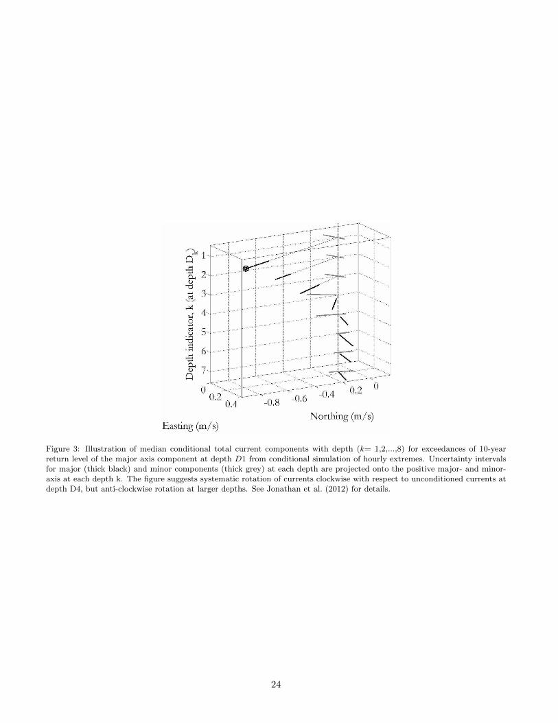
Figure 3: Illustration of median conditional total current components with depth (k= 1,2,...,8) for exceedances of 10-yearreturn level of the major axis component at depth D1 from conditional simulation of hourly extremes. Uncertainty intervalsfor major (thick black) and minor components (thick grey) at each depth are projected onto the positive major- and minor-axis at each depth k. The figure suggests systematic rotation of currents clockwise with respect to unconditioned currents atdepth D4, but anti-clockwise rotation at larger depths. See Jonathan et al. (2012) for details.
24

Figure 4: Northern North Sea location and directional sectors with distinctive wave characteristics.
25

Figure 5: Scatter plots of associated TP against storm peak HS for different directions of arrival.
26

Figure 6: Return values of storm peak HS (inner circle) and associated conditional values of TP (outer circle). Inner dashedlines (on common scale): storm peak HS with non-exceedance probability 0.99 (in 34 years), with (white) and without (black)directional effects. Outer solid lines (on common scale): median associated TP with (white) and without (black) directionaleffects; outer dashed lines give corresponding 2.5% and 97.5% percentile values for associated TP . Design values are withheldfor reasons of confidentiality.
27