1

Joint Transmit and Circuit Power Minimization inMassive MIMO with Downlink SINR Constraints:

When to Turn on Massive MIMO?Kamil Senel, Member, IEEE, Emil Bjornson, Member, IEEE, and Erik G. Larsson Fellow, IEEE

Abstract—In this work, we consider the downlink of a multi-cell multiple-input multiple-output (MIMO) system and findthe jointly optimal number of base station (BS) antennas andtransmission powers that minimize the power consumption whilesatisfying each user’s effective signal-to-interference-and-noise-ratio (SINR) constraint and the BSs’ power constraints. Differentfrom prior work, we consider a power consumption modelthat takes both transmitted and hardware-consumed power intoaccount. We formulate the joint optimization problem for bothsingle-cell and multi-cell systems. Closed-form expressions forthe optimal number of BS antennas and transmission powers arederived for the single-cell case. The analysis for the multi-cell casereveals that increasing the number of BS antennas in any cellalways improves the performance of the overall system in termsof both feasibility and total radiated power. A key contribution ofthis work is to show that the joint optimization problem can berelaxed as a geometric programming problem that can be solvedefficiently. The solution can be utilized in practice to turn on andoff antennas depending on the traffic load variations. Substantialpower savings are demonstrated by simulation.

Index Terms—Massive MIMO, power minimization.

I. INTRODUCTION

Massive multiple-input multiple-output (MaMIMO) is aphysical layer technology in which the BSs are equipped witha large number of antennas [2]. This allows MaMIMO systemsto spatially multiplex tens of users on the same time-frequencyresources, which greatly enhances the spectral efficiency of thenetwork [3]. Furthermore, simple signal processing techniques,such as linear precoding and detection schemes, are close tooptimal due to the quasi-orthogonality of the channels [4].These features makes MaMIMO a key technology for futurewireless networks [5].

A crucial design criterion for 5G systems is improved en-ergy efficiency [6]. For MaMIMO systems, it has been shownthat the required downlink transmission power to maintain aconstant SINR is inversely proportional to the number of BSantennas [7]. However, the total power consumption does notnecessarily decrease with increased number of antennas when

c©2019 IEEE. Personal use of this material is permitted. Permission fromIEEE must be obtained for all other uses, in any current or future media,including reprinting/republishing this material for advertising or promotionalpurposes, creating new collective works, for resale or redistribution to serversor lists, or reuse of any copyrighted component of this work in other works.

Parts of this work will be presented at the IEEE Wireless Communicationsand Networking Conference (WCNC), 2018 [1].

The authors are with the Department of Electrical Engineering, (ISY),Linkoping University, Sweden.

This work was supported by ELLIIT and the Swedish Foundation forStrategic Research (SSF).

using a realistic power consumption model that also takes thehardware-consumed power into account [8], [9].

There are various studies on the energy efficiency ofMaMIMO systems, which is commonly defined as the ratiobetween data rate and the power consumption. Numerical anal-ysis has shown that MaMIMO systems have the potential toimprove the energy efficiency up to a factor of 1000 comparedto a setup with typical LTE BSs [10]. For a given uplinksum rate, the optimal numbers of BS antennas and users areinvestigated for a single-cell system in [11]. However, the costof acquiring channel state information (CSI) is ignored, whichcan lead to misleading results. Another work that considers theenergy efficiency problem with perfect CSI at the receiversand provides an iterative approach is [12]. In [13], the jointuplink-downlink energy efficiency is maximized with respectto the number of BS antennas, data rate, number of users,and transmission powers. In a multi-cell setup, the energyefficiency optimization problem with respect to the numberof BS antennas is investigated in [14], which assumes perfectCSI. The total power consumption for a single-cell systemis minimized in [15] under a low traffic assumption. Theseprior works can provide general insights into the deploymentof energy-efficient networks, but when the network is in place,one cannot optimize the data rates or number of users—theseare given by the actual user traffic.

When the traffic load is low, the energy efficiency of amultiantenna systems can be increased by utilizing only asubset of the available BS antennas, referred to as antennaselection. Such an approach allows the BS to utilize only theantennas that, for the current small-scale fading realization,provide a high contribution to the SNR. An overview ofMIMO systems with antenna selection is presented in [16].Antenna selection based on small-scale fading realization wasrecently studied in the context of MaMIMO [17], [18]. Ithas been shown that antenna selection provides a significantincrease in capacity when the number of antennas is greaterthan RF chains and perfect CSI is available [19]. A geneticalgorithm for antenna selection that is capable of optimizingdifferent objective functions is proposed in [20]. In [21], asubset of the antennas is selected in a decentralized mannerby the receiving users under a setup with imperfect CSI. Aniterative water-filling scheme for antenna selection is presentedin [22]. A detailed comparison of antenna selection approachesis presented in [23]. In principle, the unselected antennascan be turned off to save energy, but in wideband systemswith many subcarriers it is unlikely that a certain antenna is

arX

iv:1

711.

1026

9v3

[cs

.IT

] 2

1 Fe

b 20

19

2

simultaneously unselected on all subcarriers; thus, antennascan generally not be turned off. Furthermore, antenna selectionbased on small-scale fading realizations requires all antennasto be turned on during the channel estimation, thus the sleeptime is very short.

In this work, we consider the downlink of a MaMIMOsystem and minimize the total power consumption by jointlyoptimizing the transmission powers and the number of activeantennas, with given constraints on the maximum transmitpower, the required effective SINRs, and available numberof antennas. The optimization is based on the large-scalefading coefficients, not the small-scale fading realizations,which enables us to turn off antennas to save power when thetraffic load is low. For downlink precoding, maximum ratiotransmission (MRT) and zero-forcing (ZF) are considered.A conference version of this work has been presented at[1], where only a single-cell setup is considered. This papercontains more general and complete results for the single-cell case along with the investigation of multi-cell setups. Tosummarize, the main contributions of this work are as follows:• The number of BS antennas and transmission powers

are jointly optimized, while satisfying individual powerand SINR constraints for both single-cell and multi-cell setups. The feasibility conditions are manifestedanalytically. The problem can be infeasible for a givennumber of antennas, but always becomes feasible as thenumber of antennas increases for a single-cell system.(Lemmas 1-2)

• We provide closed-form expressions for the optimumnumber of antennas and transmission powers when us-ing MRT or ZF precoding for a single-cell system.We compare these schemes analytically and numerically.(Theorem 2, Lemma 5)

• We prove that increasing the number of BS antennasin any cell does not deteriorate the performance of theoverall system. (Lemma 7)

• For the multi-cell case, we reformulate the joint optimiza-tion problem as a geometric programming problem thatcan be solved efficiently.

A. Organization and Notation

Vectors and matrices are denoted by boldface lowercase anduppercase letters, respectively. The superscripts (·)T and (·)Hrepresent the transpose and conjugate transpose. IN is the N×N identity matrix. The inverse of a matrix A is denoted byA−1 and r(A) is its spectral radius. R,Z are the sets of realnumbers and integers whereas the strictly positive integers arerepresented by Z+. The trace operator is denoted by tr(·) and‖ · ‖ is used for the Euclidean norm. The (i, j)-th element ofa matrix A is denoted by aij and similarly the mth elementof a vector is described by [a]m. For matrices/vectors �,�operators are used for component-wise inequalities.

The rest of the paper is organized as follows. The systemsetup is introduced in Section II. The single-cell setup isinvestigated in Section III, including the closed-form solutionfor the joint optimization problem. In Section IV, the resultsare extended to multi-cell systems and the joint optimization

problem is reformulated as a geometric programming problem.The numerical analysis is presented in Section V and SectionVI concludes the paper.

II. SYSTEM SETUP

We consider a massive MIMO system with L cells, indexedby l, and each cell has a BS with Ml active antennas,out of Mmax available antennas. Cell l contains K single-antenna users that simultaneously communicate with the BS.The system operates in time-division duplex (TDD) mode,where time-frequency resources are divided into coherenceintervals, such that each channel is constant and frequency-flatin each interval. The channels are assumed to take independentrealizations in each coherence interval from stationary ergodicprocesses. A coherence interval consists of three phases:uplink data transmission, uplink training, and downlink datatransmission. In this paper, we focus on the uplink trainingand downlink data transmission, while we leave uplink datatransmission analysis as future work.

Let N denote the length of the coherence interval (insamples) and assume that Np < N samples are used for uplinktraining. The remaining N−Np samples are used for downlinkdata transmission. During the training, the users simultane-ously transmit their pilot sequences, which are known to BSand the channels are estimated based on the received signals.As in practice, the active user set and the corresponding SINRconstraints in a given coherence interval are assumed to bedetermined by a preceding MAC-layer process.

III. SINGLE CELL SYSTEM

We first analyze a single-cell system and extend the resultsto multi-cell systems in Section IV. Since we consider asingle cell, we drop the cell index in this section. In thetraining phase, the users concurrently transmit Np-length pilotsequences. The pilot sequences are assumed to be orthogonaland therefore the length must be greater than the number ofusers, i.e., Np ≥ K. The channel between user k and the BSis represented by

gk =√βkhk (1)

where βk denotes the large-scale fading and hk is the M × 1vector representing the small-scale fading. The elements ofhk are assumed to be i.i.d. CN(0, 1). The large-scale fadingis assumed to be known at BS whereas the small-scalefading is to be estimated in each coherence interval1. Theminimum mean square estimator (MMSE) is utilized to obtainan estimate of gk [26]. Since the channels are statisticallyidentical across all antennas, the mean square of the channelestimate is same for all m ∈ {1, . . . ,M} and for the mthcomponent it is given by

γk =Npρulβ

2k

1 +Npρulβk. (2)

where ρul denotes the uplink SNR.

1Real measurements performed with both uniform linear array and uniformcylindrical array antennas reveal that correlation between antennas yields onlya minor penalty on the maximum rate of the users compared to the i.i.d.Rayleigh fading case [24], [25].

3

In the downlink, the BS precodes and scales the datasymbols to generate the transmit signal. Throughout this work,we only consider zero-forcing and maximum-ratio transmis-sion. Although there are other methods capable of achievingsomewhat better SINRs [29], closed-form expressions of theeffective SINRs for these methods are only available in theasymptotic region. Furthermore, ZF and MRT are nearlyoptimal when M � K under high and low SINR conditions,respectively [2]. Let pk be the normalized transmission powerfor user k, then the effective SINR is given by

SINRMRTk =

Mγkpk

1 + βk∑Kk′=1 pk′

(3)

for MRT and

SINRZFk =

(M −K) γkpk

1 + (βk − γk)∑Kk′=1 pk′

(4)

for ZF. Note that the “effective SINR” corresponds to the SNRof an additive white Gaussian noise (AWGN) channel withequivalent capacity, such that log2(1 + SINR) is an ergodicachievable rate [27], [28]. Further details on the derivation for(3) and (4) are given in [2], [32].

In a communication system each user has a quality-of-service (QoS) requirement determined by the user applicationand it must be satisfied by allocating system resources. QoSrequirements may depend on various different parameters suchas latency, rate, SINR, jitter, etc. In this work, we assume theserequirements are in the form of effective SINRs, i.e., each userk has a desired SINR αk > 0 such that the QoS requirementis

SINRk ≥ αk. (5)

This is equivalent to having a rate constraint of log2(1 +αk).In practice, the value of αk will change over time and it isimportant to have an efficient scheme to reallocate resourceswhen this happens.

A system is called feasible if it is possible to satisfy theSINR requirements of each user simultaneously for a givenM with a positive power vector p = [p1, p2, . . . , pk]T andinfeasible otherwise. The system resources to be allocated arethe number of BS antennas, M and the transmit powers, p.This is a generalization of prior works, in which the numberof antennas is usually constant.

Combining (3) for k = 1, . . . ,K with (5), we obtain(MIK −TF

)p ≥ ν (6)

where ν =[α1

γ1, . . . , αk

γk

]Tis the normalized noise vector,

T = [tij ] ∈ RK×K is a diagonal matrix given by

tij =

{αi, if i = j,

0, otherwise,(7)

and F = [fij ] ∈ RK×K is a rank one matrix with

fij =

{βi

γi, for MRT,

βi−γiγi

, for ZF,(8)

and

M =

{M, for MRT,M −K, for ZF.

(9)

Notice that M must be a positive integer, hence for ZFprecoding M must be greater than the number of users. Themaximum M is

Mmax =

{Mmax, for MRT,Mmax −K, for ZF,

(10)

where Mmax is the maximum number of antennas available atthe BS.

If (6) is satisfied with equality, we have

p† =(MIK −TF

)−1ν (11)

which is a feasible solution (i.e., the desired SINR values canbe satisfied simultaneously with a positive p) if and only ifthe spectral radius of TF, denoted by r(TF), is less than M .Furthermore, for the feasible case, the solution given by p† isthe unique minimum power vector, i.e., any p 6= p† satisfying(5) requires at least as much power component-wise [33], [34].

First, consider the power optimization problem

minimizep�0,M∈Z+

K∑k=1

pk

subject to SINRk ≥ αk,M ≤ Mmax,K∑k=1

pk ≤ ρd,

(P1)

where ρd is the maximum transmit power of the BS. AlthoughM is not explicitly included in the objective function, it is alsoan optimization parameter that affect the SINRs.

For a given M , the minimum power solution to (P1) isgiven by (11) if the system is feasible. Moreover, since (11)provides the minimum power solution, it must be the solutionto (P1) and satisfy the power constraints. Otherwise, (P1) hasno solution with the given power constraints for the givenM . An important property of multi-antenna systems is that,contrary to single-antenna systems, the number of antennas isalso a variable that can be optimized. We consider the problemof finding not only the optimal p, but the optimal (M,p)-pairfor (P1).

An important property of (P1) is that even without the powerconstraints the feasibility of the problem is not guaranteedand depends on the number of antennas, desired SINRs, andthe ratios βi

γi= 1 + 1

Npρulβk, which is an indicator of the

channel estimation quality. The desired SINRs and βi

γiare

fixed, whereas the number of BS antennas is an optimizationparameter. Some results on the feasibility of the problem isprovided below.

Lemma 1: Assume the problem defined by (P1) is infeasiblefor M = Mmax, then there exists no (p, M) pair whichprovides a solution to (P1).

Proof: Rewriting (11), we have

p† =1

M

(IK −B(M)

)−1ν, (12)

4

where B(M) = 1MTF.

Let the pair (p′, M ′) be a feasible solution to (P1) whereM ′ < Mmax, then r(B(M ′)) < 1 ≤ r(B(Mmax)).However, B(M ′) � B(Mmax) which implies r(B(M ′)) ≥r(B(Mmax)) [35, Corollary 8.1.19] and contradicts with theassumption that (p′, M ′) is a feasible solution.

This result suggests that it is impossible to turn an infeasiblesystem into a feasible one by reducing the number of antennas.Next, a simple extension of Lemma 1 is stated without proof.

Lemma 2: Let (p, M) be a pair that satisfies the SINRconstraints defined in (6), then there exist at least one p′ vectorfor any M ′ > M such that (p′, M ′) also satisfies the SINRconstraints.

The preceding analysis manifests the effect of changing thenumber of antennas on the feasibility of the system. However,the solution to (P1) must minimize the transmission powersamong all possible solutions in the feasible set.

Theorem 1: Consider the problem defined by (P1) andassume that there exists at least one feasible solution. Let thepair (p∗, M∗) denote the optimal solution to the problem, thenM∗ = Mmax and p∗ =

(MmaxIK −TF

)−1ν.

Proof: First, we need to show that for any (p′, M ′) pairwith M ′ < Mmax satisfying (6), we have p′ � p∗, where p∗ isthe minimum power solution corresponding to M∗ = Mmax.Recall that for a given M the minimum power solution isgiven by (11). Hence, it is sufficient to compare the resultingpower vectors using (11) which satisfies the SINR constraints(6) with equality, i.e.,(

MmaxIK −TF)p∗ = (M ′IK −TF)p′. (13)

Since M ′ < Mmax, the equality implies p′ � p. Since, withincreasing M , the transmission powers can be reduced and itis not possible to turn a feasible system into an infeasible oneby increasing the number of antennas, as shown in Lemma 2,we have M∗ = Mmax. Finally, the optimal power vector isgiven by (11) which concludes the proof.

This theorem proves that one should keep all antennas onin a MaMIMO system to minimize the transmission power,which is rather intuitive given the power-scaling laws in [7].

Remark 1: The solution provided by Theorem 1 is valid forboth precoding schemes, MRT and ZF. However, the exactvalues of the optimal solution are different since M and Fare defined differently. Furthermore, the feasibility of oneprecoding scheme does not imply the feasibility of the other.

Fig. 1 illustrates the change on the required transmissionpower as a function of the number of BS antennas, for differentnumbers of users uniformly distributed in a circular cell andZF precoding. The simulation parameters for the numericalanalysis provided throughout the paper are summarized inthe Table I. For this particular example, the SINR target isαk = 1 for each user. A low value is chosen to guarantee thefeasibility of the system when the number of antennas is small.As expected, Fig. 1 shows that the total power decreases withincreasing number of antennas, which verifies the precedinganalysis. The figure also shows that, as the number of usersincreases, the required total transmission power increases.Note that the gain from increasing M is very significant whenM is small but diminishes as M grows. Furthermore, the total

0 20 40 60 80 10010

−4

10−3

10−2

10−1

100

Number of Antennas (M)

Total

Transm

ission

Pow

er(W

)

K = 20K = 10K = 5

Fig. 1. Total transmission power as a function of number of BS antennas forvarious number of users.

transmission power grows faster than linear with respect to Kand decreases linearly with M , which is in alignment with theresults provided in [9].

So far, the cost of increasing the number of antennas hasbeen neglected. In a practical system, using more antennas hasa cost in terms of increased circuit power [10], [12]. Hence,a more practical consumption model is

c1M + c2

K∑k=1

pk (14)

where c1 ≥ 0 is the circuit power consumption per antennaand c2 > 1 represents the amplifier inefficiency factor whichaccounts for power dissipation in the amplifiers. The values ofc1 and c2 depends on the hardware quality deployed at the BS,operational frequency, quantization bits. The expected powerconsumption per antenna is 300 mW and the power amplifierhas 30% efficiency. These numbers are subject to technologicalscaling. Especially, the consumption per antenna reduces bya factor of two for every technology generation (every twoyears) [8], [9].

The joint optimization problem based on the consumptionmodel in (14) is

minimizep�0,M∈Z+

c1M + c2

K∑k=1

pk

subject to SINRk ≥ αk,M ≤ Mmax,K∑k=1

pk ≤ ρd.

Consider the following equivalent optimization problem,which is obtained by dividing the cost function by c2 anddefining the relative power cost of operating each antenna,

5

c = c1/c2,

minimizep�0,M∈Z+

cM +

K∑k=1

pk

subject to SINRk ≥ αk,M ≤ Mmax,K∑k=1

pk ≤ ρd.

(P2)

Note that we have also replaced M with M in the costfunction, which does not change the solution.2 Obviously, theoptimal solution depends on c and (P2) reduces to (P1) whenc = 0.

Let

U(p, M) = cM +

K∑k=1

pk (15)

denote the cost function for a given (p, M) pair. Beforewe state our main result for single-cell systems, we firstinvestigate the required number of antennas such that the SINRconstraints can be satisfied and state the following.

Lemma 3: Let MSINRmin be the minimum number of antennas

such that (11) results in a positive power vector that satisfiesthe SINR constraints given in (5). Then, MSINR

min = dM cSINRmin e

whereM cSINR

min = tr(TF). (16)

Proof: Recall that (11) provides a feasible solution if andonly if the spectral radius of TF is less than M . TF is a rank-one matrix and r(TF) = tr(TF). Hence, M cSINR

min ≥ r(TF) =tr(TF).Lemma 3 shows that the number of active antennas can beadjusted based on the traffic load of the system as MSINR

min

depends on the large-scale coefficients, channel estimationquality and target SINR levels.

The transmission powers are shown to decrease as thenumber of antennas increases in Theorem 1. Next, we derivethe minimum number of antennas required to satisfy the bothpower and SINR constraints of the joint optimization problemdefined in (P2).

Lemma 4: Consider the problem defined in (P2) and letMmin be the minimum number of antennas required to satisfyboth the SINR and power constraints. Then, Mmin = dM c

minewhere

M cmin =

1

ρd

K∑k′=1

αk′

γk′+ tr(TF). (17)

Proof: The power constraint can be written as

ρd ≥K∑k=1

pk (18)

= 1Tp (19)

= 1T(MIK −TF

)−1ν (20)

=1

M1T(IK +

1

M − tr(TF)TF

)ν (21)

2 Note that for ZF precoding, the first term of the cost function in (P2) isequal to c(M −K). Since cK is a constant term, the problem is equivalentto the one with cM and both problems have identical optimal solutions.

where (20) and (21) follows from (11) and Lemma 11,respectively. Finally (17) can be obtained by solving for M in(21). Note that M c

min > tr(TF) as α, γ and ρd are all strictlypositive variables. Hence, we have M c

min > M cSINRmin which

implies Mmin ≥ MSINRmin and Mmin = dM c

mine.Lemma 4 reveals the minimum required number of antennas

such that (P2) has a solution. This provides a lower boundon the optimum number of antennas. The main result for thesingle-cell systems regarding (P2) is stated below.

Theorem 2: Assume that there exists at least one (p, M ′)-pair that satisfies the constraints in (P2) with M ′ ≤ Mmax andlet (p∗, M∗) denote the optimal solution with M∗ ∈ R+, then

M∗ = min(Mmax,max(M†, Mmin)), (22)

where

M† = tr(TF) +

(1

c

K∑k′=1

αk′

γk′

)1/2

(23)

andp∗ =

1

M∗

(IK +

1

M∗ − tr(TF)TF

)ν. (24)

Proof: First, note that for a given M ≥ Mmin, thetransmit powers that minimize U(p, M) are given by (11).Hence, U(M) = U(p, M) can be considered a function ofonly M , given by

U(M) = cM + 1Tp

= cM + 1T(MIK −TF

)−1ν. (25)

Using (58), (25) can further be simplified as

U(M) = cM +1

M1T(IK +

1

M − tr(TF)TF

)ν

= cM +1

M

(τ +

tr(TF)

M − tr(TF)τ

)(26)

where

τ = 1Tν =

K∑k′=1

αk′

γk′. (27)

It is straightforward to show that U(M) is a strictly convexfunction with respect to M by examining the second derivativeof (26). Therefore, the optimal solution can be found by takingthe derivative of U(M) with respect to M and equating it tozero. Let µ = tr(TF), then

d U(M)

d M= c− τ

M2− µτ(2M − µ)

M2(M − µ)2(28)

which should be equal to zero when M = M†. Rearrangingthe terms we get

cM4 − 2µcM3 + (cµ2 − τ)M2 = 0 (29)(M − µ

)2=

τ

c. (30)

In (29), two zero roots are discarded as they correspond toM = 0. From (30), we get the possible solutions M = µ±

√τc

and the optimal solution is

M† = µ+

√τ

c(31)

6

20 40 60 80 10010

-1

100

101

102

103

Fig. 2. Cost function as a function of number of BS antennas for 10 users withvarious c values and MRT precoding. For each curve, the black × representthe optimal cost function value obtained by M† defined by (31).

as M = µ−√

τc corresponds to an infeasible system.

The optimal solution given by M† must satisfy the con-straints and therefore must be greater than Mmin. For thecase where max(Mmin, M

†) > Mmax, the optimal solutionis clearly M∗ = Mmax as U(M) is a convex function of M .

Remark 2: In Theorem 2, the integer constraint on M isrelaxed and the resulting optimal M is not necessarily aninteger. However, it is clear that the optimal M is either bMcor dMe as a result of the convexity of the cost function.

In Fig. 2, power consumption for various c values and MRTprecoding (M = M ) are depicted. In each trial, the optimalpower vector for the given M is obtained using (11) andU(p,M) is computed. Each point represents the average of5000 independent trials with uniformly random user locationsand the crosses (×) represent the average of M† computed by(31) and the corresponding U(p,M†). For each c, U(p,M†)is less than the minimum obtained. However, an importantpoint is that M† is not necessarily an integer whereas thecurves are obtained by using integer M values. As c decreases,the resulting cost functions decrease and the minimum isattained at a higher M as expected. It is only when c is smallthat it is optimal to turn all antennas on, while in other casesone can save energy by turning antennas off.

Next, we investigate the relation between the optimum Mfor MRT and ZF.

Lemma 5: Consider the problem defined by (P2) and letM†MRT and M†ZF denote the optimum M ∈ R+ for MRT andZF processing such that Mmin ≤ M ≤ Mmax, respectively.Then,

M†MRT − M†ZF =

K∑k′=1

αk′ −K. (32)

Proof: The difference M†MRT − M†ZF can be computed

by substituting the definitions of F and M for MRT and ZF

1 5 10 15 20 250

10

20

30

40

50

60

70

80

Number of Users (K)

Number

ofAntennas(M

)

MMRC , α = 0.5

MMRC , α = 2

MZF , α = 0.5

MZF , α = 2

MMRC and MZF , α = 1

Fig. 3. Comparison of the optimal number of antennas for (P2) with MRTand ZF as a function of number of users.

from (8) and (9) into (23), which gives

M†MRT − M†ZF =

K∑k′=1

αk′βk′

γk′−

(K∑k′=1

αk′

(βk′

γk′− 1

))−K.

This can be simplified to obtain (32).For the case when all users have the same SINR require-

ments, i.e., αk = α for all k, (32) reduces to M†MRT−M†ZF =

K(α − 1). If α = 1, then the optimal number of antennas isequal for both approaches assuming that the optimal numberof antennas is smaller or equal to Mmax. MRT requires moreantennas for α > 1 and vice versa.

Fig. 3 illustrates the optimum number of antennas for (P2)for MRT and ZF processing with c = 0.001. The integerconstraint is relaxed to obtain the smooth curves depicted inthe figure. The optimal number of antennas for MRT is lowerwhen α < 1, it is lower for ZF when α > 1, and equalwhen α = 1, which is in alignment with Lemma 5. In all ofthe considered cases, it is optimal to turn off a subset of theantennas. If MaMIMO is defined as a system with at least50 active antennas, then we need to have tens of users and/orhigh QoS constraints to make MaMIMO optimal.

Note that (32) allows us to also compare the two precodingtechniques in a setup with heterogeneous SINR requirementsand find the optimal number of antennas. It can be concludedthat if the average SINR target is smaller than 1, MRT resultsin fewer required antennas at the optimal solution and viceversa.

IV. MULTI-CELL SYSTEM

In this section, we extend the single-cell analysis in theprevious section to a multi-cell setting, where both inter-celland intra-cell interference are considered. Furthermore, it isusually not feasible to assign orthogonal pilot sequences toevery user in the system, which results in pilot contaminationthat deteriorates the channel estimation quality and leads tocoherent interference. We consider a setup where each BSserves K users and each user is associated with a single BS.We assume that the users in a cell have mutually orthogonal

7

SINRZFlk =

(Ml −K) γllkplk

1 +K∑k′=1

( ∑l′∈Pl

pl′k′(βl

′lk − γl

′lk

)+∑l′ /∈Pl

pl′k′βl′lk

)+

∑l′∈Pl\{l}

(Ml′ −K)γl′lkpl′k

(37)

pilots while the pilot sequences of two distinct cells areeither completely orthogonal or replicated. The cells whichassign identical pilot sequences to their users causes pilotcontamination to each other. The pilot contaminating cellscause coherent interference that grows with the number ofantennas, which is a crucial difference from single-cell systemswhere the interference terms are independent of the numberof antennas.

A. Uplink Training and Downlink Data Transmission

We adopt the notation from [2]. Let gjlk denote the channelbetween user k in cell l and BS j. Then, BS l receives thesignal

Yl =√Npρul

L∑l′=1

K∑k′=1

gll′k′ϕHl′k′ + Z (33)

where ϕlk denotes the pilot sequence of user k in cell l. Inorder to estimate gllk, BS l performs a de-spreading processon the received signal as follows

y′lk = Ylϕlk

=√Npρul

L∑l′=1

K∑k′=1

gll′k′ϕHl′k′ϕlk + z′. (34)

The MMSE estimate of gllk based on (34), is denoted by gllkand contains Ml identically distributed components CN(0, γllk)with

γllk =Npρul

(βllk)2

1 +Npρul∑Ll′=1

∑Kk′=1 β

ll′k′ |ϕHl′k′ϕlk|2

, (35)

where βjlk denote the large-scale fading coefficient [26]. Notethat the summation term in the denominator contains only theterms originating from the users with identical pilot sequences.The channel estimation error with MMSE, gllk = gllk − gllk,is independent of the estimate and its elements are i.i.d. withCN(0, βllk − γllk).

Similar to the single-cell case, we consider MRT and ZFprecoding. Let Pl denote the set of cells that share the samepilot sequences with cell l including the own cell, then theeffective SINR for MRT is [2], [30], [31], [32],

SINRMRTlk =

Mlγllkplk

1 +L∑l′=1

K∑k′=1

pl′k′βl′lk +

∑l′∈Pl\{l}

Ml′γl′lkpl′k

(36)where plk is the normalized power allocation of BS l for userk and we assume that in cells with shared pilots kth usershave identical pilot sequences. Similarly for ZF, the effectiveSINR is given by (37).

First, we consider a multi-cell system with MRT and startwith the following minimization problem:

minimizep1,...,pL�0,m∈Z+

L∑l=1

K∑k=1

plk

subject to SINRlk ≥ αlk, l = 1, . . . , L, k = 1, . . . ,K

Ml ≤Mmax, l = 1, . . . , LK∑k=1

plk ≤ ρd, l = 1, . . . , L.

(P3)where pl = [pl1, . . . , plK ]T denotes the transmission powervector for BS l and m = [M1, . . . ,ML]T is the vector withthe number of active antennas at each BS. Note that we haveassumed the same power constraint for all BSs and the powerconsumption of each BS contribute equally to the objectivefunction. The QoS requirement of user k in cell l is αlk > 0.

Combining the SINR constraints

SINRlk ≥ αlk (38)

with (36) and (37), and considering all cells in the system, weobtain

(M−TF−TAM)p ≥ v (39)

in vector notation. Here p = [p1, . . . ,pL]T is the power

vector, v =[α11

γ111, α12

γ112, . . . , αLK

γLLK

]Tis the normalized noise

vector,

M =

M1

M20

. . .0

ML

(40)

with each Mi = MiIK is a diagonal matrix where

Mi =

{Mi, for MRT,Mi −K, for ZF,

(41)

T = [tij ] ∈ RLK×LK is a diagonal matrix with

tij =

{αi′j′ , if i = j,

0, otherwise,(42)

where i′ = d iK e and j′ = (j − 1) modK + 1;F = [fij ] ∈ RLK×LK with

fij =βj

′

i′k′

γi′i′k′

, ∀i, j, (43)

for MRT and

fij =

βj′

i′k′

γi′i′k′

, if j′ /∈ Pi′ ,

βj′

i′k′−γj′

i′k′

γi′i′k′

, if j′ ∈ Pi′ ,(44)

8

for ZF. Here, i′ = d iK e, j′ = d jK e and k′ = (i−1) modK+1;

A = [aij ] ∈ RLK×LK with

aij =

γj′

i′k′′

γi′i′k′

, if k′ = k′′ and j′ ∈ Pi′\{i′},

0, otherwise,(45)

where i′ = d iK e, j′ = d jK e, k

′ = (i − 1) modK + 1 andk′′ = (j − 1) modK + 1 for both MRT and ZF.

It is straightforward to show that the optimal solution to(P3) is obtained when the SINR constraints are satisfied withequality. Hence, the minimum power solution is

p = (M−TF−TAM)−1v, (46)

if and only if the spectral radius of TFM−1 + TA is lessthan unity. The solution in (46) guarantees that the SINRconstraints are satisfied for all users. Furthermore, it is theminimum power solution, i.e., any other solution satisfying(38) requires at least as much power component-wise [34].This implies that if the solution given in (46) does not satisfythe power constraints in (P3), there exist no other powervector that satisfies the SINR and power constraints in (P3),simultaneously. Contrary to the single-cell case, in the multi-cell case there is a coherent interference term in (38) that scaleswith the number of BS antennas in the pilot-sharing cellswhich limits the SINRs of the system. Before we investigatethe effect of coherent interference on the system and theinterplay between the number of BS antennas and transmissionpowers, a brief introduction to M-matrices is provided.

Definition 1: Let A be a square matrix with nonpositiveoff-diagonal elements and nonnegative diagonal entries, thenA can be expressed as

A = sI−B, (47)

where s > 0 and B is a nonnegative matrix. Furthermore,assume that s > r(B), then A is a nonsingular M-matrix[36].Next, we summarize some of the properties of M-matriceswhich will be utilized in the succeeding analysis.

Lemma 6: Let A be a square matrix, then the followingstatements are equivalent [36, Chapter 6]:• A is a nonsingular M-matrix.• A−1 exists and A−1 � 0.• A is a monotone matrix, i.e., for all real vectors x, Ax �

0⇒ x � 0.The feasibility conditions based on the spectral radius of TFin single-cell case and TF+TAM in multi-cell case actuallycorrespond to the resulting matrix being an M-matrix.

In order to obtain the solution to (P3), we need to investigatethe interplay between the number of antennas and the transmis-sion powers. Although it is clear that increasing the number ofantennas in cell l will result in a smaller transmission powervector pl for cell l, the effect on the overall system is notclear, since the number of antennas also appear in the coherentinterference term. Next, we address this problem and state thefollowing.

Lemma 7: Consider the problem defined by (P3) and let(m1,p1), (m2,p2) be two solutions satisfying (38) withequality. If m1 �m2, then p1 � p2.

Proof: Since the SINR constraints are satisfied withequality, we have

(Mm1−TF−TAMm1

)p1 = (Mm2−TF−TAMm2

)p2

(48)where Mm1 , Mm2 are the antenna matrices defined in (40)for the corresponding m1 and m2. Let N = Mm1 −Mm2 bea diagonal matrix denoting the difference. It is a non-negativematrix since m1 �m2 and (48) can be simplified as(

ILK −TFM−1m2−TA

)−1(ILK −TA)Np1 =

Mm2(p2 − p1) . (49)

The left-hand side of (49) is non-negative since(ILK −TFM−1

m2−TA

)−1(ILK −TA) =

ILK +(ILK −TFM−1

m2−TA

)−1TFM−1

m2(50)

and(ILK −TFM−1

m2−TA

)is an M-matrix. Then, the non-

negativity of left-hand side of (49) implies that p2 − p1 � 0.

Lemma 7 reveals that the total transmission power can bereduced by increasing the number of antennas. Furthermore,increasing the number of antennas in one cell also resultsin a lower total transmission power. This shows that evenin the presence of coherent interference the overall systemperformance can be improved by increasing the number ofantennas of BSs.

Lemma 8: Let (m1,p1) be a pair satisfying (38). Then, thereexists at least one p′ for any m′ �m1 such that (m′,p′) alsosatisfies (38).

Proof: Note that T,F,A are all non-negative matricesand

TFM−1m′ + TA � TFM−1

m1+ TA. (51)

Since (m1,p1) satisfies (38), using [35, Corollary 8.1.19], wecan obtain

r(TFM−1m′ + TA) ≤ r(TFM−1

m1+ TA) < 1. (52)

which concludes the proof.Lemma 8 shows that it is not possible to turn a feasible

system into an infeasible one by increasing the number of an-tennas, similar to single-cell case. Furthermore, combined withLemma 7, a system with increased number of antennas willalso require less transmission power. Unfortunately, Lemmas 7and 8 do not imply that a feasible solution can always be foundby increasing the number of BS antennas. Next, we considerthe feasibility of the system with respect to the number ofantennas and state the following.

Lemma 9: Consider the problem defined by (P3) and assumethat r(TA) ≥ 1, then, there exist no (m,p) pair that satisfiesthe SINR constraints given in (38).

Proof: Recall that the SINR constraints given in (38) canconcurrently be satisfied if and only if the spectral radius ofTFM−1 + TA is less than unity. Notice that

TFM−1 + TA � TA (53)

which implies that

r(TFM−1 + TA

)≥ r (TA) , (54)

9

as all of the matrices are non-negative. Although increasingthe number of antennas will reduce the spectral radius ofTFM−1 +TA, even in the asymptotic region where the num-ber of antennas approaches infinity the term due to coherentinterference, TA, does not vanish. Hence, it is not possible tomake the system feasible.

A crucial difference between the single-cell and multi-cell setups is revealed in Lemma 9. In the single-cell case,TA = 0 and it is always possible to make a system feasibleby increasing the number of antennas whereas in a multi-cellsystem this is not the case. This phenomenon is a result ofthe coherent interference caused by pilot contamination, whichdoes not vanish with increasing M and limits the achievableSINRs. The maximum SINR that can be concurrently achievedby all users is summarized in the following lemma.

Lemma 10: Consider a multi-cell system with M1 =M2 . . . = ML = M and let α∗ denote the maximum SINRthat can be achieved by all users. Then,

0 < α∗ ≤ 1

r(A)(55)

and equality is satisfied only as M →∞.Proof: It is clear that α∗ is lower bounded by 0. As M →

∞, the non-coherent interference term TFM−1 vanishes andfor a feasible system r (TA) must be less than unity. Thisgives the upper bound on the α∗ stated in (55).An interesting property of the two precoding schemes isrevealed by Lemma 10. In the asymptotic region, MRT andZF give the same max-min SINR solution which agrees withthe asymptotic analysis given in [2, Section 4.4.1].

Remark 3: For a multi-cell system with orthogonal pilotsassigned to each user, there is no coherent interference and itis possible to reach a feasible system for any target value byincreasing the number of antennas (assuming Mmax =∞) inthe system similar to single cell case.

Next, we state the main result for the problem defined in(P3).

Theorem 3: Consider the problem defined in (P3) andassume that there exists at least a feasible solution for Ml =Mmax for all l. Then, M∗ = Mmax and

p∗ = (Mmax −TF−TAMmax)−1v (56)

where Mmax is the antenna matrix with each diagonal elementequal to Mmax.

Proof: The results of Lemma 7 suggests that increasingthe number of antennas results in a lower transmission powervector and it has been shown that it is impossible to transforma feasible system into an infeasible one by increasing thenumber of antennas. Hence, using the maximum number ofantennas at each BS will give us the solution to the problemdefined in (P3).

The problem of minimizing only the total transmissionpower in the system results in a solution which requires to usethe maximum number of BS antennas in multi-cell systems,similar to the Theorem 1 in the single-cell case. The totaltransmission power as a function of number of antennas isdepicted in Fig. 4 for a setup with MRT. However, the problem

0 20 40 60 80 10010

−5

10−4

10−3

10−2

10−1

100

Maximum Number of Antennas (Mmax )

Total

Transm

ission

Pow

er(W

)

K = 20

K = 10

K = 5

Fig. 4. Total transmission power of the optimal solution to (P3) as a functionof Mmax.

becomes more challenging when the cost of utilizing antennasis included in the cost function which is examined next.

The joint optimization problem which also includes a costfor utilizing BS antennas is

minimizep1,...,pL�0,m∈Z+

c1

L∑l=1

K∑k=1

plk + c2

L∑l=1

Ml

subject to SINRlk ≥ αlk, l = 1, . . . , L, k = 1, . . . ,K

Ml ≤Mmax, l = 1, . . . , LK∑k=1

plk ≤ ρd, l = 1, . . . , L.

Consider the following equivalent optimization problem,which can be obtained by dividing the cost function by c2 andutilizing the relative cost of operating each antenna, c = c1/c2,

minimizep1,...,pL�0,m∈Z+

L∑l=1

K∑k=1

plk + c

L∑l=1

Ml

subject to SINRlk ≥ αlk, l = 1, . . . , L, k = 1, . . . ,K

Ml ≤Mmax, l = 1, . . . , LK∑k=1

plk ≤ ρd, l = 1, . . . , L.

(P4)It is clear from Theorem 3 that increasing number of anten-

nas results in a lower transmission power vector. However, thisis not necessarily the optimal solution to (P4) as there is a costassociated with utilizing antennas. Contrary to the single-cellcase, it is not possible to obtain a closed-form expression forthe solution to (P4). In principle, we can use (46) to solve (P4),as it allows us to find the optimal power vector for a given m.Considering each m in the search space requires examining(Mmax − 1)L combinations and the corresponding optimalpower vector, then choosing the minimum among them wouldresult in finding the optimal solution to (P4). However, thisexhaustive search would not be scalable with L and may notbe suitable for practical applications.

Fortunately, the problem defined by (P4) can be relaxed asa geometric programming (GP) problem for which the optimal

10

solution can be obtained very efficiently and reliably. In orderto solve the optimization problem, the required informationis on the large scale-coefficients and the SINR constraints. Inpractice, the GP problem can either be solved by a central unitwhich conveys the solution to the BSs or each BS can obtainthe solution by acquiring the required information from otherBSs. A brief introduction to GP is provided in the AppendixB and further details can be found in [37].

The objective function of (P4) is a posynomial and it isstraightforward to modify all of the constraints except theSINR constraint to obtain a problem at a standard GP form.For the SINR constraint, taking the inverse of the inequality,we obtain

1 +L∑l′=1

K∑k′=1

pl′k′βll′k +

∑l′∈Pl\{l}

Ml′γll′kpl′k

Mlγllkplk≤ 1

αlk, (57)

for MRT. The left-hand side of (57) is a posynomial. For thecase with ZF, the SINR constraints can also be formulatedas posynomials in a similar way. Hence, the problem definedby (P4) can be relaxed as a geometric programming problemwhich can be solved effectively even for many users andlarge number of antennas. Using the inverse of the SINR totransform the SINR constraints into posynomial constraintshave previously been utilized for power control problems toreformulate them as geometric programming problems [37],but not for the type of problems that we consider here.Similar to the single-cell case the integer constraint on m isrelaxed and m is assumed to be a real-valued vector in theGP problem. In practice, the real-valued vector obtained viasolving the GP problem must be converted to an integer-valuedvector.

V. NUMERICAL ANALYSIS

In this section, we present the numerical analysis for themulti-cell case which not only verifies the preceding theoreti-cal analysis, but also provides valuable insight for the designof MaMIMO systems. The simulations were performed usingMatlab with CVX and the code will be made available online.

For the multi-cell simulations, we consider the cellular setupillustrated in Fig. 5. There are L = 16 cells that are distributedon a 4×4 square grid with a wrap-around topology. Each cellserves K users that are distributed uniformly in the 250 m ×250 m area. There is a minimum distance, dmin between usersand their serving BS. The rest of the simulation parameters aresummarize in Table I.

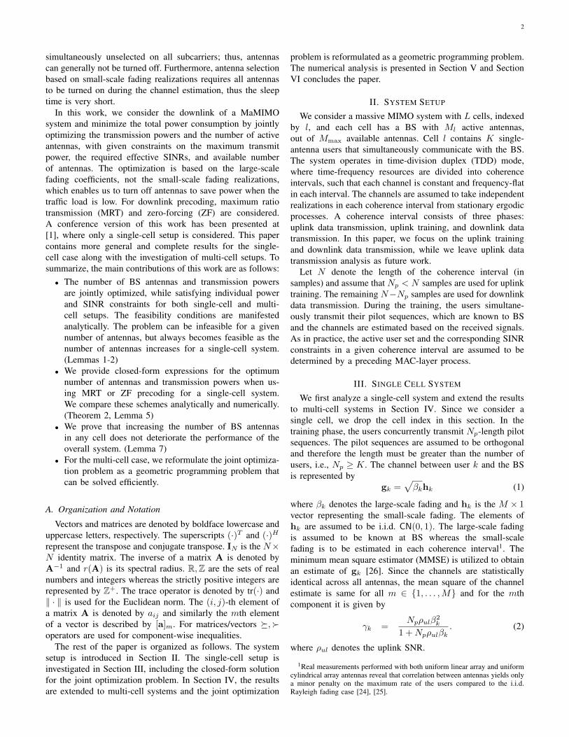
Fig. 6 illustrates the max-min SINR achieved by MRT andZF for various number of BS antennas. In this particularexample, each BS is assumed to have an identical numberof antennas. As expected, the achievable max-min SINRincreases with the number of BS antennas. However, thisincrease is limited due to the coherent interference and thereis a finite maximum SINR that can be achieved as M → ∞as proved by Lemma 10. Fig. 6 also provides an empiricalstudy for the feasibility of a system at a given M and targetSINR. For example, with M = 150 and target SINR α = 1.5,on average 30% of the realizations will be infeasible. This is

9 10 11 12

13 14 15 16

1 2

5 6

9 10

13 14

9 10

13 14

3 4

7 8

11 12

15 16

11 12

15 16

1 2

5 6

1 2 3 4

5 6 7 8

3 4

7 8

An arbitrary cell

0.25 km

1 2 3 4

5 6 7 8

9 10 11 12

13 14 15 16

Fig. 5. Multi-cell setup with cells distributed on a square grid.

TABLE ISIMULATION PARAMETERS

System Parameter ValuePath and penetration loss at distance d (km) 130 + 37.6 log10(d)Bandwidth (Bw) 20 MHzCell Edge Length (dedge) 250 mMinimum Distance (dmin) 15 mNumber of Cells (L) 16Total Noise Power (Bwσ2) 2·10−13 WMaximum DL-Transmission Power (ρd) 1 WUL-Transmission Power (ρul) 0.1 WRelative Pilot Length: Np/K 1Maximum number of BS antennas (Mmax) 100

a consequence of the random user locations and fixed SINRvalue we selected; in practice, the MAC-layer is responsiblefor assigning feasible SINR values to the users. Anotherimportant point is the performance of the different precoders.MRT provides a better performance when M is low whereasZF achieves a better performance at higher M .

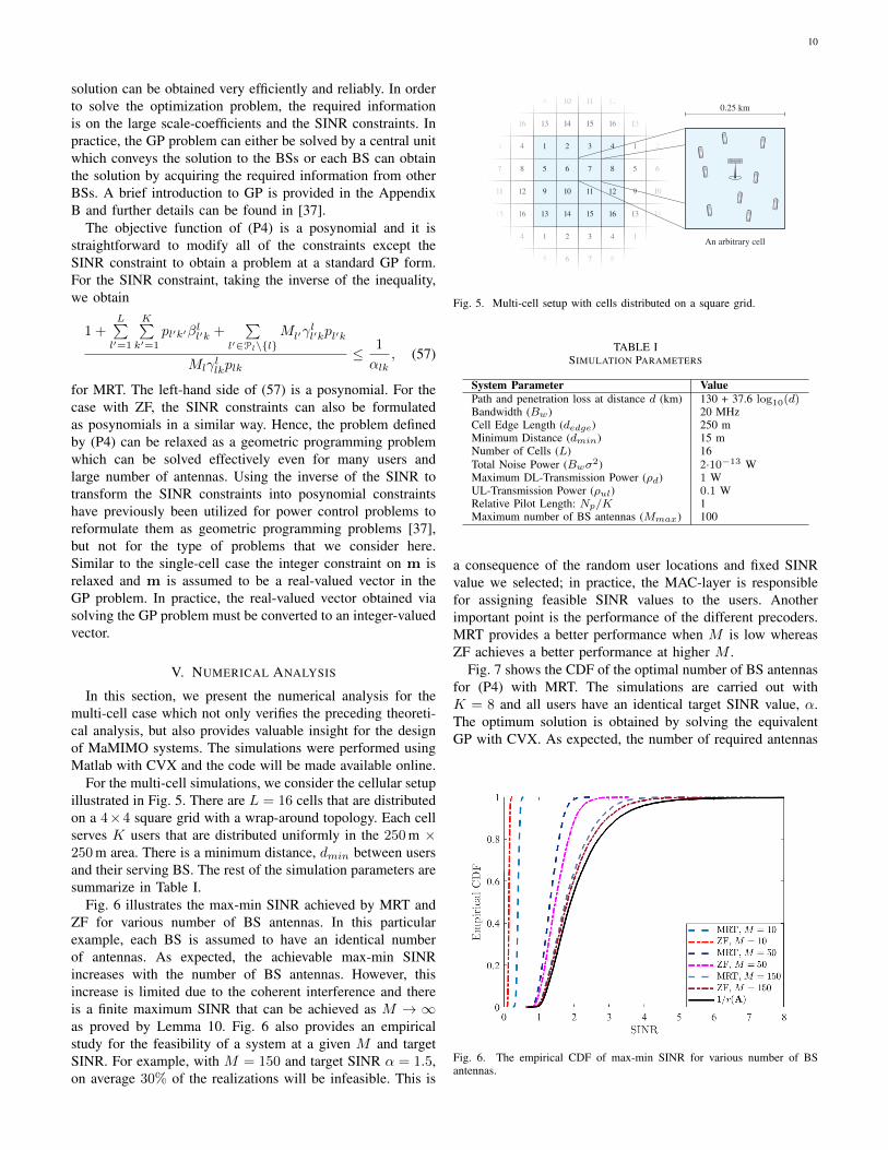
Fig. 7 shows the CDF of the optimal number of BS antennasfor (P4) with MRT. The simulations are carried out withK = 8 and all users have an identical target SINR value, α.The optimum solution is obtained by solving the equivalentGP with CVX. As expected, the number of required antennas

Fig. 6. The empirical CDF of max-min SINR for various number of BSantennas.

11

0 20 40 60 80 1000

0.2

0.4

0.6

0.8

1

Number of BS antennas (M )

EmpiricalCDF

α = 0.5

α = 1

α = 1.5

Fig. 7. The empirical CDF of the optimal number of BS antennas for (P4)with MRT.

increases as the target SINR value is increased. Note that someof the trials resulted in an infeasible system for the given targetSINR and those trials were discarded.

10−4

10−3

10−2

10−1

100

10−2

100

102

104

Relative Power Cost (c)

U(m

∗,p

∗)an

dD(m

∗,m

max)

D(m∗,mmax)

U (m∗,p∗)

Fig. 8. The difference between the cost functions for m = mmax and theoptimal solution along with the cost function of the optimal solution withrespect to the relative power cost for (P4).

Let D(m1,m2) = |U(m1,p1) − U(m2,p2)| be the dif-ference between the two cost function for m1 and m2 (andthe corresponding optimum power vectors). Fig. 8 depicts theoptimal solution to (P4) obtained via geometric programmingalong with the difference between the optimum solution andthe solution obtained by utilizing the maximum number of an-tennas, i.e., U(m∗,p∗) and D(m∗,mmax). There are K = 8users in each cell and MRT precoder is used. The differencebetween the optimal solution and the solution with maximumnumber of antennas increases with the relative power cost, asexpected. For the case where utilizing more antennas has nocost (c = 0), the optimum solution is utilizing the maximumnumber of antennas at each BS. Assuming a system with300 mW power consumption per antenna and 30% poweramplifier efficiency, c = 0.09. It is also important to notethat based on past trends, the power consumption per antennascales with a factor of two for each technology generation,whereas the power amplifier efficiency does not benefit fromthe technological advancements at the same scale which leads

to a smaller c value and suggest increased number of BSantennas in future cellular systems [8], [9].

101

102

103

104

0

0.2

0.4

0.6

0.8

1

Fig. 9. The difference between the cost functions with the integer solutionm = dm∗e and the optimal solution m∗ for different relative cost values.

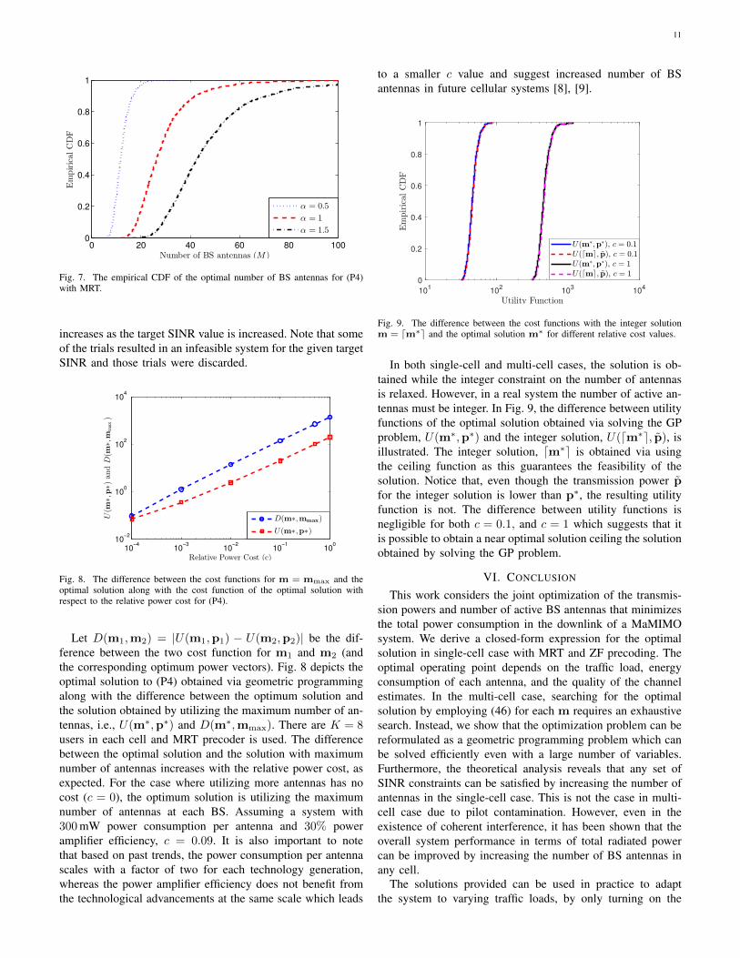
In both single-cell and multi-cell cases, the solution is ob-tained while the integer constraint on the number of antennasis relaxed. However, in a real system the number of active an-tennas must be integer. In Fig. 9, the difference between utilityfunctions of the optimal solution obtained via solving the GPproblem, U(m∗,p∗) and the integer solution, U(dm∗e, p), isillustrated. The integer solution, dm∗e is obtained via usingthe ceiling function as this guarantees the feasibility of thesolution. Notice that, even though the transmission power pfor the integer solution is lower than p∗, the resulting utilityfunction is not. The difference between utility functions isnegligible for both c = 0.1, and c = 1 which suggests that itis possible to obtain a near optimal solution ceiling the solutionobtained by solving the GP problem.

VI. CONCLUSION

This work considers the joint optimization of the transmis-sion powers and number of active BS antennas that minimizesthe total power consumption in the downlink of a MaMIMOsystem. We derive a closed-form expression for the optimalsolution in single-cell case with MRT and ZF precoding. Theoptimal operating point depends on the traffic load, energyconsumption of each antenna, and the quality of the channelestimates. In the multi-cell case, searching for the optimalsolution by employing (46) for each m requires an exhaustivesearch. Instead, we show that the optimization problem can bereformulated as a geometric programming problem which canbe solved efficiently even with a large number of variables.Furthermore, the theoretical analysis reveals that any set ofSINR constraints can be satisfied by increasing the number ofantennas in the single-cell case. This is not the case in multi-cell case due to pilot contamination. However, even in theexistence of coherent interference, it has been shown that theoverall system performance in terms of total radiated powercan be improved by increasing the number of BS antennas inany cell.

The solutions provided can be used in practice to adaptthe system to varying traffic loads, by only turning on the

12

number of antennas required to deliver the requested trafficwith minimal power consumption. The uplink analysis couldpotentially provide similar insights and will be considered forfuture work.

APPENDIX AMATRIX INVERSION LEMMA

The following is a special case of the Matrix inversionlemma (also known as Sherman-Morrison-Woodbury lemma)[35, pg. 19].

Lemma 11: Let B be a rank one matrix, then

(I−B)−1

= I +1

1− tr(B)B. (58)

APPENDIX BGEOMETRIC PROGRAMMING

This appendix provides a brief introduction to GP mainlybased on [37]. In order to model the optimization problemsintroduced in this paper, the following definitions are required.

A function is called monomial if it is of the form

f(x) = κxa11 xa22 . . . xann (59)

where κ > 0 and x = [x1, x2, . . . , xn]T is a vector withreal positive components. The exponents a1, a2, . . . , an arereal valued but not necessarily positive. A function is calledposynomial if it can be represented as a sum of one or moremonomial functions, i.e.,

f(x) =

K∑k=1

κkxa1k1 xa2k2 . . . xank

n (60)

is a posynomial. Note that, addition and multiplication of aposynomial with another one results in a posynomial. Fur-thermore, division of a posynomial by a monomial gives aposynomial.

An optimization problem of the form

minimize f0(x)

subject to fi(x) ≤ 1, i = 1, . . . , n,

gi(x) = 1, i = 1, . . . , l,

(61)

is called a standard form GP if fi are posynomial functionsand gi are monomial functions of optimization variable x. Ifan optimization problem is reduced to the standard form GP,it can be effectively solved by any GP software. In this work,CVX is used [38].

REFERENCES

[1] K. Senel, E. Bjornson, E. G. Larsson, “Adapting the Number of Antennasand Power to Traffic Load: When to Turn on Massive MIMO?”, submittedto IEEE Wireless Communications and Networking Conference (WCNC),2018.

[2] T. L. Marzetta, E. G. Larsson, H. Yang and H. Q. Ngo, “Fundamentalsof Massive MIMO”, Cambridge University Press, 2016.

[3] E. G. Larsson, and L. Van der Perre. ”Massive MIMO for 5G.” IEEE 5GTech Focus 1, no. 1 (2017).

[4] E. Bjornson, E. G. Larsson, and T. L. Marzetta, “Massive MIMO:Ten myths and one critical question”, IEEE Communications Magazine,vol. 54, no. 2, pp. 114–123, 2016.

[5] J. G. Andrews, S. Buzzi, W. Choi, S. V. Hanly, A. Lozano, A. CK. Soong,and J. C. Zhang, “What will 5G be?”, IEEE Journal on selected areasin communications, vol. 32, no. 6, pp. 1065–1082, 2014.

[6] K. N. R. S. V. Prasad, E. Hossain, and V. K. Bhargava, “Energy Efficiencyin Massive MIMO-Based 5G Networks: Opportunities and Challenges”,IEEE Wireless Communications, 2017.

[7] J. Hoydis, S. T. Brink, and M. Debbah, “Massive MIMO in the UL/DLof cellular networks: How many antennas do we need?”, IEEE Journalon selected Areas in Communications, vol. 31, no. 2, pp. 160–171, 2013.

[8] C. Desset, and B. Debaillie, “Massive MIMO for energy-efficient com-munications”, European Microwave Conference, pp. 138–141, 2016.

[9] C. Desset, B. Debaillie, and F. Louagie, “Modeling the hardware powerconsumption of large scale antenna systems”, IEEE Online Conferenceon Green Communications, pp. 1–6, 2014.

[10] H. Yang, and T. L. Marzetta, “Total energy efficiency of cellular largescale antenna system multiple access mobile networks”, in Proc. IEEEOnline Green Communications, pp. 27–32, 2013.

[11] S. K. Mohammed, “Impact of transceiver power consumption on theenergy efficiency of zero-forcing detector in massive MIMO systems”,IEEE Transactions on Communications, vol. 62, no. 11, pp. 3874–3890,2014.

[12] D. W. K. Ng, E. S. Lo, and R. Schober, “Energy-efficient resource allo-cation in OFDMA systems with large numbers of base station antennas”,IEEE Transactions on Wireless Communications, vol. 11, no. 9, pp. 3292–3304, 2012.

[13] E. Bjornson, L. Sanguinetti, J. Hoydis, and M. Debbah, “Optimal designof energy-efficient multi-user MIMO systems: Is massive MIMO theanswer?”, IEEE Transactions on Wireless Communications, vol. 14, no. 6,pp. 3059–3075, 2015.

[14] M. M. Hossain, C. Cavdar, E. Bjornson, and R. Jantti, “Energy Effi-ciency of Massive MIMO: Coping with Daily Load Variation”, [Online].Available: https://arxiv.org/abs/1512.01998

[15] H. V. Cheng, D. Persson, E. Bjornson, and E. G. Larsson, “MassiveMIMO at night: On the operation of massive MIMO in low traffic sce-narios”, In IEEE International Conference on Communications, pp. 1697–1702, 2015.

[16] A. F. Molisch, and M. Z. Win, “MIMO systems with antenna selection”,IEEE microwave magazine, vol. 5, no. 1, pp. 46–56, 2004.

[17] M. Arash, E. Yazdian, and M. Fazel, “Employing Antenna Selection toImprove Energy-Efficiency in Massive MIMO Systems”, 2017, [Online].Available: https://arxiv.org/abs/1701.00767

[18] B.- J. Lee, S. -L. Ju, N. Kim, and K. -S. Kim, “Enhanced Transmit-Antenna Selection Schemes for Multiuser Massive MIMO Systems”,Wireless Communications and Mobile Computing, 2017.

[19] X. Gao, O. Edfors, J. Liu, and F. Tufvesson, “Antenna selection inmeasured massive MIMO channels using convex optimization”, In IEEEGlobecom Workshops, pp. 129–134, 2013.

[20] B. Makki, A. Ide, T. Svensson, T. Eriksson, and M. -S. Alouini, “AGenetic Algorithm-Based Antenna Selection Approach for Large-but-Finite MIMO Networks”, IEEE Transactions on Vehicular Technology,vol. 66, no. 7, pp. 6591–6595, 2017.

[21] M. Benmimoune, E. Driouch, W. Ajib, and D. Massicotte, “Noveltransmit antenna selection strategy for massive MIMO downlink channel”,Wireless Networks, vol. 23, no. 8, pp. 2473–2484.

[22] J. Xu, and L. Qiu, “Energy efficiency optimization for MIMO broadcastchannels”, IEEE Transactions on Wireless Communications, vol. 12,no. 2, pp. 690-701, 2013.

[23] N. P. Le, and F. Safaei, “Antenna selection strategies for MIMO-OFDMwireless systems: An energy efficiency perspective”, IEEE Transactionson Vehicular Technology, vol. 65, no. 4, pp. 2048–2062, 2016.

[24] X. Gao, O. Edfors, F. Rusek, and F. Tufvesson, “Massive MIMOperformance evaluation based on measured propagation data”, IEEETransactions on Wireless Communications, vol. 14, no. 7, pp. 3899–3911,2015.

[25] F. Rusek, D. Persson, B. K. Lau, E. G. Larsson, T. L. Marzetta,O. Edfors, and F. Tufvesson, “Scaling up MIMO: Opportunities andchallenges with very large arrays”, IEEE signal processing magazine,vol. 30, no. 1, pp. 40–60, 2013.

[26] S. M. Kay, “Fundamentals of statistical signal processing, volume I:estimation theory”, Prentice Hall, 1993.

[27] G. Caire, “On the ergodic rate lower bounds with applications to massiveMIMO”, IEEE Transactions on Wireless Communications, vol. 17, no. 5,pp. 3258–3268, 2018.

[28] H. Q. Ngo, E. G. Larsson, and T. L. Marzetta, “Energy and spectralefficiency of very large multiuser MIMO systems”, IEEE Transactionson Communications, vol. 61, no. 4, pp. 1436–1449, 2013.

13

[29] E. Bjornson, M. Bengtsson and B. Ottersten, “Optimal multiuser transmitbeamforming: A difficult problem with a simple solution structure”, IEEESignal Processing Magazine, vol. 31, no. 4, pp. 142–148, 2014.

[30] A. Ashikhmin and T. L. Marzetta, “Pilot contamination precoding inmulti-cell large scale antenna systems”, IEEE International Symposiumon Information Theory Proceedings, pp. 1137–1141, 2012.

[31] H. Yang and T. L. Marzetta, “Total energy efficiency of cellularlarge scale antenna system multiple access mobile networks”, OnlineConference on Green Communications, pp. 27–32, 2013.

[32] T. V. Chien, and E. Bjornson, “Massive MIMO Communications”, 5GMobile Communications, Springer, pp. 77–116, 2017,

[33] Pillai, S. Unnikrishna, Torsten Suel, and Seunghun Cha. ”The Perron-Frobenius theorem: some of its applications.” IEEE Signal ProcessingMagazine 22, no. 2 (2005): 62-75.

[34] N. Bambos, S. C. Chen, and G. J. Pottie, “Channel access algorithmswith active link protection for wireless communication networks withpower control”, IEEE/ACM Transactions On Networking, vol. 8, no. 5,pp. 583-597, 2000.

[35] R. A. Horn and C. R. Johnson, “Matrix analysis”. Cambridge universitypress, 2012.

[36] A. Berman and R. J. Plemmons, “Nonnegative matrices in the mathe-matical sciences”, Society for Industrial and Applied Mathematics, 1994.

[37] S. Boyd, S. J. Kim, L. Vandenberghe and A. Hassibi, “A tutorial ongeometric programming”, Optimization and engineering, vol. 8, no. 1,2007.

[38] M. Grant and S. Boyd, CVX: Matlab software for disciplined convexprogramming, version 2.0 beta. http://cvxr.com/cvx.