João Rafael Cardoso de Brito Oliveira Abrantes

INFRARED THERMOGRAPHY AS A GROUND-BASED

SENSING TOOL TO ASSESS SURFACE HYDROLOGIC

PROCESSESS

Doctoral Thesis in Civil Engineering, in the scientific area of Hydraulics, Water Resources and Environment, supervised by Professor João Luís Mendes Pedroso de

Lima and Professor Abelardo Antônio de Assunção Montenegro (UFRPE, Brazil), and submitted to the Department of Civil Engineering of the Faculty of Sciences and

Technology of the University of Coimbra.

August 2019

Faculty of Sciences and Technology of the University of Coimbra

Department of Civil Engineering

INFRARED THERMOGRAPHY AS A

GROUND-BASED SENSING TOOL TO

ASSESS SURFACE HYDROLOGIC PROCESSES

João Rafael Cardoso de Brito Oliveira Abrantes

Doctoral Thesis in Civil Engineering, in the scientific area of Hydraulics, Water Resources and

Environment, supervised by Professor João Luís Mendes Pedroso de Lima and Professor Abelardo

Antônio de Assunção Montenegro (UFRPE, Brazil), and submitted to the Department of Civil

Engineering of the Faculty of Sciences and Technology of the University of Coimbra.

August 2019

Dedicated to the persons I love the most in this world:

my grandmother Fernanda

my parents Cristina and Manel

my sister Mariana

my brother Tomás

“The foolish man seeks happiness in the distance, the wise grows it under his feet.”

- James Oppenheim

“There will come a time when you believe everything is finished. That will be the beginning.”

- Louis L'Amour

Infrared thermography as a ground-based sensing tool to assess surface hydrologic processes i

ACKNOWLEDGEMENTS

I would like to express my gratitude and respect to my supervisors, without whom this Thesis would

not have been possible. To Professor João Pedroso de Lima, whose creativity, imagination and

inventiveness fostered my interest in scientific research. Professor João directly contributed to my

success, by acknowledging my capacities, investing his time and resources in me, providing the so

needed availability, patience, guidance and support whenever required and by transmitting to me

his immense knowledge and insatiable thirst for science. To Professor Abelardo Montenegro, who

believed in me and gave me the opportunity to work alongside him after completing my master’s

degree. For sure, that was a crucial moment that defined the following years. Professor Abelardo

whose cooperation, knowledge and advises contributed to this Thesis and my, still short, research

career. Thank you very much Professors for the supervision, but, above all, for the friendship.

I am thankful for the positive environment comprised of professors, researchers and colleagues that

was indispensable to the fulfilment of this Thesis. To Professor Isabel Pedroso de Lima, Doctor

Jacob Keizer, Professor Alexandre Silveira, Professor Rodrigo Moruzzi, Professor Nuno Simões

and Professor Jorge Isidoro, for their expertise, cooperation and motivation throughout these years.

To Raquel, Valdemir, Sérgio and Iraê for their help in the laboratory experiments. To Babar,

Cleene, Isabela, Marcelle, Mousinho and Nazmul for their company and fun moments in the

laboratory. To the laboratory technician Mr. Joaquim Cordeiro, for his suggestions, creativity and

talent during the design and construction of some installations used in the experiments. Also, thanks

for the pearls of wisdom learned during our lively talks.

To my closer friends (you know who you are) for the trusty words during the not so good times,

the so much needed leisure and fun moments and, above all, the endless long-time friendship.

Last but not least, I would like to express my eternal love and gratitude to my family for their

unconditional care, dedication and support expressed all over my life. To my grandmother Fernanda

for all the affection and tenderness, to my parents Cristina and Manel for all the sacrifices they

made to give me everything I could ask for, to my siblings Mariana and Tomás for their friendship

and for instilling in me an almost paternal sense of responsibility, to my aunts Lucinda, Guiga and

Gigi for being like second-mothers to me, to my cousins Teresa, Verónica and Artur, and, of course,

to my beloved buddy Baloo.

To all: THANK YOU VERY MUCH!

Infrared thermography as a ground-based sensing tool to assess surface hydrologic processes iii

FINANCIAL AND INSTITUTIONAL SUPPORT

The research presented in this Thesis was supported by the Doctoral grant SFRH/BD/103300/2014,

financed by Foundation for Science and Technology (FCT), Portugal, through the National

Strategic Reference Framework (QREN) and the Human Potential Operational Program (POPH),

co-financed by the European Social Fund (ESF).

The research was also partially supported by the:

• Project PTDC/ECM/105446/2008, “Experimental and Numerical set-up for validation of the

Dual-Drainage (sewer/surface) concept in an Urban Flooding Framework”, and Project

PTDC/ECM-HID/4259/2014 – POCI-01-0145-FEDER-016668, “HIRT - Modelling surface

hydrologic processes based on infrared thermography at local and field scales”, financed by

the Foundation for Science and Technology (FCT), Portugal, through the Operational

Programme ‘Thematic Factors of Competitiveness’ (COMPETE), co-financed by the

European Regional Development Fund (ERDF);

• Strategic project UID/MAR/04292/2013, granted to MARE- Marine and Environmental

Sciences Centre, Portugal, financed by the Foundation for Science and Technology (FCT);

• Project “RECARE - Preventing and Remediating degradation of soils in Europe through

Land Care" (Grant Agreement 603498), financed by the European Union (EU);

• Project “Estudo do desempenho de tecnologias para a conservação de água e solo no

Semiárido”, within the Special Visiting Researcher program (Process 400757/2013-3),

finance by the National Council of Scientific and Technological Development of the

Ministry of Science and Technology (CNPq/MCT), Brazil, through the Science Without

Borders program;

• Project “Análise de diferentes padrões de precipitação em estudos hidrológicos e

conservacionistas em parcelas no Semiárido” (Process PBPG-1532-5.03/13), within the call

FACEPE 14/2013, and Project “Pesquisa e tecnologias hídricas para o desenvolvimento do

Semiárido de Pernambuco” (Process APQ-0300-5.03/17), within the call FACEPE 04/2017,

financed by the Pernambuco State Research Support Foundation (FACEPE), Brazil;

• COST Action CA16219, ”HARMONIOUS - Harmonization of UAS techniques for

agricultural and natural ecosystems monitoring”, financed by the European Cooperation in

Science and Technology (COST), through the EU Framework Programme Horizon 2020.

iv Infrared thermography as a ground-based sensing tool to assess surface hydrologic processes

Researchers from the following institutions were involved in the research:

• MARE - Marine and Environmental Sciences Centre, Portugal;

• CESAM - Centre for Environmental and Maritime Studies, Aveiro, Portugal;

• Department of Civil Engineering of the Faculty of Sciences and Technology of the

University of Coimbra (FCTUC), Coimbra, Portugal;

• Department of Environment and Planning of the University of Aveiro (DAO/UA), Aveiro,

Portugal;

• Department of Agricultural Engineering, Rural Federal University of Pernambuco

(DEAGRI/UFRPE), Recife, PE, Brazil;

• Institute of Science and Technology, Federal University of Alfenas (ICT/UNIFAL-MG),

Poços de Caldas, MG, Brazil.

Infrared thermography as a ground-based sensing tool to assess surface hydrologic processes v

ABSTRACT

The harmful impacts of surface runoff and associated water erosion on the environment and

populations have been widely recognized throughout the history. Understanding and modelling

these processes is, therefore, of crucial importance for engineers, scientists and policy makers in

the field of Hydraulics, Water Resources and Environment, in order to predict beforehand their

impacts and develop proper protection and conservation policies and technologies. Attempts to

understand and investigate such processes encompass laboratory experiments, field monitoring and

numerical modelling. Each one of these approaches has its purpose, advantages and disadvantages.

One thing they all have in common is the necessity of cost-effective techniques to obtain good

quality hydrologic data. A recent technological boost in infrared thermography has drawn the

attention of the scientific community to the development and investigation of innovative

measurement techniques based on these systems. However, not all the potential of these systems

has been exploited so far and investigation is still needed.

The aim of this Thesis was to develop innovative techniques based on infrared thermography that

can be used as sensing tools to assess different morphologic and hydraulic characteristics of the

soil surface and flowing water, and investigate if the collected information can be useful to model

and better understand surface hydrologic processes, namely surface runoff and water erosion.

The research developed in this doctoral study started by the development of innovative techniques

based on infrared thermography to assess the morphology of the soil surface (microrelief and rills)

and soil surface hydraulic characteristics (permeability, macroporosity, water repellency). These

techniques were firstly developed in laboratory controlled conditions, in scenarios where some

more common measuring techniques cannot be applied successfully. A follow up study to

investigate the applicability of these techniques to assess soil water repellency in real field

conditions was then carried out. Afterwards, the research focused on the investigation of thermal

tracers to estimate basic hydraulic characteristics of shallow flows. The thermal tracer technique

was compared to other more tradicional tracer techniques, such as dye and salt. A numerical

approach to handle data from thermal tracers as an alternative method to estimate the velocity of

shallow flows was then explored. This was done by fitting an analytical solution of an advection–

dispersion transport equation to temperature data from thermal tracers. Finally, a two-dimensional

(2D) numerical model of surface runoff, infiltration and water erosion was developed. The model

combines the two-dimensional unsteady water flow equations on an infiltrating surface with a two-

dimensional sediment transport equation, distinguishing between rill erosion, interrill erosion and

sediment deposition. Numerical simulations were validated with data from laboratory rainfall

simulation experiments on a bi-directional soil flume.

vi Infrared thermography as a ground-based sensing tool to assess surface hydrologic processes

The research presented in this doctoral study revealed that infrared thermography can be used as a

ground-based sensing tool for acquisition of information on soil surface characteristics and flow

hydraulics. These techniques have shown great potential to: i) Estimate the spatial variability of

soil surface morphology where other techniques cannot be applied (presence of organic residues

concealing the soil surface); ii) Estimate the spatial variability of soil surface hydraulic

characteristics in a faster and expedite way, instead of multiple time-consuming point

measurements that need to be grouped or scaled to bring out spatial coherence; and iii) Estimate

the surface flow velocity in the occurrence of very shallow flows where many measurement

equipment cannot be used.

One big advantage of these techniques is the possibility of qualitative real time monitoring of the

spatial dynamics of some key processes in surface hydrology, using only one infrared camera.

However, in quantitative terms, the precision of some of these techniques relies on measurements

with other more common techniques. As usual, such novel sensing tools will require extensive

calibration and validation to be routinely adopted in field monitoring practices.

Observations from these techniques can be used to complement observations from other techniques.

Also, techniques and equipment can be combined; e.g. dual cameras with optical and infrared

sensors to combine both type of observations, infrared cameras couple with unmanned aerial

vehicles to combine observations at different spatial scales.

No doubt, the information collected with these techniques can be useful to calibrate and validate

numerical models of surface hydrology, such as surface runoff and water erosion, as well as to

better understand the underlying processes.

Keywords Surface hydrology; Measurement techniques; Infrared camera; Surface runoff; Water erosion;

Numerical model

Infrared thermography as a ground-based sensing tool to assess surface hydrologic processes vii

RESUMO

São conhecidos os vários impactos negativos do escoamento superficial e da erosão hídrica no meio

ambiente e nas populações. Entender e modelar esses processos é, portanto, crucial para

engenheiros, cientistas e responsáveis políticos na área da Hidráulica, Recursos Hídricos e

Ambiente. Investigações desses processos abrangem desde experiências de laboratório,

monitorizações de campo e modelações numéricas. Todas estas abordagens têm em comum a

necessidade de técnicas economicamente viáveis para a obtenção de dados hidrológicos de boa

qualidade. O recente salto tecnológico em termografia por infravermelhos tem chamado a atenção

da comunidade científica para o desenvolvimento e investigação de técnicas inovadoras de medição

baseadas nesses sistemas. No entanto, até ao momento, o seu potencial ainda não foi completamente

explorado, sendo ncessário mais investigação.

Esta Tese teve como objetivo principal o desenvolvimento de técnicas inovadoras baseadas em

termografia por infravermelha que possam ser usadas como ferramentas de deteção para avaliar

diferentes características morfológicas e hidráulicas da superfície do solo e do escomento

superficial, e investigar a utilidade dessa informação na melhoria da modelação e compreenção de

processos hidrológicos superficiais, nomeadamente o escoamento superficial e a erosão hídrica.

A investigação desenvolvida neste estudo de doutoramento iniciou-se com o desenvolvimento de

técnicas inovadoras baseadas em termografia por infravermelhos para avaliar a morfologia da

superfície do solo (microrrelevo e sulcos) e características hidráulicas da superfície do solo

(permeabilidade, macroporosidade e hidrofobicidade). Numa primeira fase, estas técnicas foram

desenvolvidas em condições controladas de laboratório, em situaçoes onde não é possível aplicar

com sucesso algumas técnicas de medição mais comuns. Numa segunda fase, efectuou-se um

estudo para investigar a aplicabilidade dessas técnicas para avaliar a hidrofobicidade do solo em

condições reais de campo. Posteriormente, a investigação centrou-se no estudo de traçadores

térmicos para avaliar características hidráulicas de escoamentos superficiais pouco profundos. A

técnica do traçador térmico foi comparada a outras técnicas de traçadores mais tradicionais, como

corante e sal. De seguida, explorou-se uma abordagem numérica para lidar com dados de traçadores

térmicos como um método alternativo para estimar a velocidade de escoamentos superficiais.

Finalmente, foi desenvolvido um modelo numérico bidimensional (2D) de escoamento superficial,

infiltração e erosão hídrica. O modelo combina as equações bidimensionais do escoamento numa

superfície permeável com uma equação bidimensional de transporte de sedimentos, distinguindo

entre erosão entre sulcos, erosão em sulcos e deposição de sedimentos. As simulações numéricas

foram validadas com dados experimentais de simulação de chuva em laboratório num canal de terra

bidirecional.

viii Infrared thermography as a ground-based sensing tool to assess surface hydrologic processes

A investigação apresentada neste estudo de doutoramento revelou que a termografia por

infravermelhos pode ser usada como uma ferramenta de aquisição de dados sobre as características

da superfície do solo e do escoamento superficial. Estas técnicas mostraram grande potencial no

sentido de: i) Estimar a variabilidade espacial da morfologia da superfície do solo onde outras

técnicas não podem ser aplicadas (presença de resíduos orgânicos sobre a superfície do solo);

ii) Estimar a variabilidade espacial de características hidráulicas da superfície do solo de forma

mais rápida e expedita, em vez de múltiplas medições pontuais que precisam ser agrupadas para se

obter coerência espacial; e iii) Estimar a velocidade superficial de escoamentos muito pouco

profundos, onde muitos equipamentos de medição não podem ser usados.

Uma grande vantagem destas técnicas é a possibilidade de monitorização qualitativa em tempo real

da dinâmica espacial de alguns processos chave em hidrologia de superfície, usando apenas uma

câmara de infravermelhos. No entanto, em termos quantitativos, a precisão de algumas destas

técnicas depende de medições com outras técnicas mais comuns. Como de costume, estas novas

ferramentas de deteção vão necessitar de trabalhos extensivos de calibração e validação para serem

adotadas como práticas comuns em monitorização de campo.

As observações com estas técnicas podem ser utilizadas para complementar observações de outras

técnicas. Além disso, técnicas e equipamentos podem ser combinados; por exemplo, câmaras

duplas com sensores óticos e infravermelhos para combinar observações; câmaras de

infravermelhas acopladas a veículos aéreos não tripulados para combinar observações a diferentes

escalas espaciais.

Sem dúvida, as informações obtidas com estas técnicas podem ser úteis para calibrar e validar

modelos numéricos de hidrologia de superfície, como escoamento superficial e erosão hídrica, bem

como para entender melhor os processos subjacentes.

Palavras-chave Hidrologia de superfície; Técnicas de medição; Câmara de infravermelhos; Escoamento superficial;

Erosão hídrica; Modelo numérico

Infrared thermography as a ground-based sensing tool to assess surface hydrologic processes ix

TABLE OF CONTENTS

ACKNOWLEDGEMENTS ..............................................................................................................i

FINANCIAL AND INSTITUTIONAL SUPPORT ....................................................................... iii

ABSTRACT ..................................................................................................................................... v

RESUMO ...................................................................................................................................... vii

TABLE OF CONTENTS ................................................................................................................ix

LIST OF FIGURES ........................................................................................................................ xv

LIST OF TABLES ..................................................................................................................... xxiii

1. INTRODUCTION ........................................................................................................................ 1

1.1. Framework and motivation .................................................................................................. 1

1.2. Research question and objectives ......................................................................................... 2

1.3. Thesis structure .................................................................................................................... 3

1.4. Publications .......................................................................................................................... 6

2. LITERATURE REVIEW ........................................................................................................... 11

2.1. Components and processes in surface hydrology ............................................................... 11

2.1.1. Rainfall ....................................................................................................................... 11

2.1.2. Infiltration .................................................................................................................. 12

2.1.3. Surface runoff ............................................................................................................. 13

2.2. Water erosion ..................................................................................................................... 14

2.2.1. Water erosion processes ............................................................................................. 14

2.2.2. Water erosion modelling ............................................................................................ 16

2.3. Conditioning factors in surface hydrology ......................................................................... 18

2.3.1. Rainfall characteristics ............................................................................................... 18

2.3.2. Soil surface morphology ............................................................................................ 19

2.3.3. Soil surface cover ....................................................................................................... 19

2.3.4. Soil hydraulic characteristics ..................................................................................... 21

x Infrared thermography as a ground-based sensing tool to assess surface hydrologic processes

2.4. Measurement techniques in surface hydrology ................................................................. 22

2.4.1. Rainfall characteristics .............................................................................................. 22

2.4.2. Soil surface morphology ........................................................................................... 23

2.4.3. Soil hydraulic characteristics ..................................................................................... 24

2.4.4. Flow velocity ............................................................................................................. 25

2.5. Infrared thermography ....................................................................................................... 27

2.5.1. Background, operating principles and applications ................................................... 27

2.5.2. Applications in surface hydrology............................................................................. 28

3. CAN INFRARED THERMOGRAPHY BE USED TO ESTIMATE SOIL SURFACE

MICRORELIEEF AND RILL MORPHOLOGY? ........................................................................ 37

3.1. Abstract ............................................................................................................................. 37

3.2. Introduction ....................................................................................................................... 37

3.3. Methodology...................................................................................................................... 39

3.3.1. Experimental setup .................................................................................................... 39

3.3.2. Soil surface microrelief scenarios ............................................................................. 40

3.3.3. Experimental procedure ............................................................................................ 42

3.3.4. Data analyses ............................................................................................................. 42

3.4. Results and discussion ....................................................................................................... 45

3.4.1. Scenarios with artificial rills ...................................................................................... 45

3.4.2. Scenarios with surface eroded by water .................................................................... 49

3.5. Conclusion ......................................................................................................................... 52

4. PREDICTION OF SKIN SURFACE SOIL PERMEABILITY BY INFRARED

THERMOGRAPHY: A SOIL FLUME EXPERIMENT .............................................................. 55

4.1. Abstract ............................................................................................................................. 55

4.2. Introduction ....................................................................................................................... 55

4.3. Materials and methods ....................................................................................................... 56

4.3.1. Setup .......................................................................................................................... 56

4.3.2. Experimental procedure ............................................................................................ 57

4.3.3. Data analyses ............................................................................................................. 58

4.4. Results and interpretation .................................................................................................. 59

Infrared thermography as a ground-based sensing tool to assess surface hydrologic processes xi

4.5. Conclusions ........................................................................................................................ 62

5. MAPPING SOIL SURFACE MACROPORES USING INFRARED THERMOGRAPHY: AN

EXPLORATORY LABORATORY STUDY ................................................................................ 65

5.1. Abstract .............................................................................................................................. 65

5.2. Introduction ........................................................................................................................ 65

5.3. Materials and methods........................................................................................................ 67

5.3.1. Laboratory setup ......................................................................................................... 67

5.3.2. Soil surface macropores ............................................................................................. 68

5.3.3. Experimental procedure ............................................................................................. 69

5.4. Results and discussion ........................................................................................................ 70

5.5. Conclusions ........................................................................................................................ 74

6. ASSESSING SOIL WATER REPELLENCY SPATIAL VARIABILITY USING A

THERMOGRAPHIC TECHNIQUE: AN EXPLORATORY STUDY USING A SMALL-SCALE

LABORATORY SOIL FLUME .................................................................................................... 77

6.1. Abstract .............................................................................................................................. 77

6.2. Introduction ........................................................................................................................ 77

6.3. Material and methods ......................................................................................................... 79

6.3.1. Experimental setup ..................................................................................................... 79

6.3.2. Soil water repellency (SWR)...................................................................................... 80

6.3.3. Experimental procedure ............................................................................................. 81

6.4. Results and discussion ........................................................................................................ 83

6.5. Conclusions ........................................................................................................................ 88

7. FIELD ASSESSMENT OF SOIL WATER REPELLENCY USING INFRARED

THERMOGRAPHY ....................................................................................................................... 93

7.1. Abstract .............................................................................................................................. 93

7.2. Introduction ........................................................................................................................ 93

7.3. Study area and soil surface repellency ............................................................................... 95

7.4. Infrared thermographic technique ...................................................................................... 96

7.5. Results and discussion ........................................................................................................ 97

7.6. Conclusion ........................................................................................................................ 101

xii Infrared thermography as a ground-based sensing tool to assess surface hydrologic processes

8. USING A THERMAL TRACER TO ESTIMATE OVERLAND AND RILL FLOW

VELOCITIES .............................................................................................................................. 105

8.1. Abstract ........................................................................................................................... 105

8.2 Introduction ...................................................................................................................... 105

8.3. Materials and methods ..................................................................................................... 107

8.3.1. Laboratory set-ups ................................................................................................... 107

8.3.2. Soil .......................................................................................................................... 107

8.3.3. Tracers ..................................................................................................................... 109

8.3.4. Video recording systems ......................................................................................... 109

8.3.5. Laboratory procedure .............................................................................................. 110

8.4. Results and discussion ..................................................................................................... 111

8.5. Conclusions ..................................................................................................................... 117

9. COMPARISON OF THERMAL, SALT AND DYE TRACING TO ESTIMATE SHALLOW

FLOW VELOCITIES: NOVEL TRIPLE-TRACER APPROACH ............................................ 121

9.1. Abstract ........................................................................................................................... 121

9.2. Introduction ..................................................................................................................... 122

9.3. Material and methods ...................................................................................................... 124

9.3.1. Hydraulic channel and simulated flows .................................................................. 124

9.3.2. Triple tracer ............................................................................................................. 126

9.3.3. Tracer detection systems ......................................................................................... 126

9.3.4. Data analyses ........................................................................................................... 127

9.4. Results and discussion ..................................................................................................... 131

9.4.1. Triple-tracer velocities ............................................................................................ 131

9.4.2. Advantages and disadvantages of the tracer techniques .......................................... 140

9.4.3. α and β correction factors ........................................................................................ 141

9.5. Conclusions ..................................................................................................................... 147

10. COMBINING A THERMAL TRACER WITH A TRANSPORT MODEL TO ESTIMATE

SHALLOW FLOW VELOCITIES ............................................................................................. 151

10.1. Abstract ......................................................................................................................... 151

10.2. Introduction ................................................................................................................... 152

Infrared thermography as a ground-based sensing tool to assess surface hydrologic processes xiii

10.3. Methodology .................................................................................................................. 155

10.3.1. Solute and heat transport model ............................................................................. 155

10.3.2. Analytical solution, initial and boundary conditions .............................................. 155

10.4. Experimental methodology ............................................................................................ 156

10.4.1. Setup and simulated flows...................................................................................... 156

10.4.2. Tracer techniques ................................................................................................... 158

10.4.3. Data analyses .......................................................................................................... 159

10.5. Results and discussion .................................................................................................... 161

10.6. Conclusions .................................................................................................................... 170

11. TWO-DIMENSIONAL (2D) NUMERICAL MODELLING OF RAINFALL INDUCED

OVERLAND FLOW, INFILTRATION AND SOIL EROSION: COMPARISON WITH

LABORATORY RAINFALL-RUNOFF SIMULATIONS ON A TWO-DIRECTIONAL SLOPE

SOIL FLUME ............................................................................................................................... 175

11.1. Abstract .......................................................................................................................... 175

11.2. Introduction .................................................................................................................... 176

11.3. Governing equations ...................................................................................................... 177

11.3.1. Overland flow and soil erosion .............................................................................. 177

11.3.2. Infiltration .............................................................................................................. 179

11.4. Numerical methods ........................................................................................................ 181

11.4.1. MacCormack operator-splitting scheme ................................................................ 181

11.4.2. Initial conditions ..................................................................................................... 183

11.4.3. Boundary conditions .............................................................................................. 183

11.5. Model application and simulation results ....................................................................... 184

11.5.1. Experimental tests .................................................................................................. 184

11.5.2. Model parameterisation .......................................................................................... 186

11.5.3. Model evaluation .................................................................................................... 187

11.5.4. Simulation results ................................................................................................... 187

11.6. Conclusion ...................................................................................................................... 191

12. FINAL REMARKS ................................................................................................................ 195

12.1. Conclusions .................................................................................................................... 195

xiv Infrared thermography as a ground-based sensing tool to assess surface hydrologic processes

12.2. Answer to research question .......................................................................................... 199

12.3. Future work ................................................................................................................... 200

13. REFERENCES ...................................................................................................................... 203

APPENDIX A............................................................................................................................... A.1

Infrared thermography as a ground-based sensing tool to assess surface hydrologic processes xv

LIST OF FIGURES

Figure 3.1. Sketch of the setup used in the laboratory tests (not at scale). ..................................... 39

Figure 3.2. Photographs of the soil surface of the flumes: a) Small study section with three small

artificially created rills; b) Small study section with three big artificially created rills; c) Bare soil

with microrelief created by water erosion; d) Low mulching cover; and e) High mulching cover. X

represents the distance along the width of the flumes and Y represents the distance along the length

of the flumes. .................................................................................................................................. 41

Figure 3.3. Soil surface elevation profiles of the scenarios with artificial rills: a) Scenario with three

small rills (see Figure 3.2a); b) Scenario with three large rills (see Figure 3.2b); c) Scenario with

three deep rills; and d) Scenario with a combination of three rills with different sizes. X represents

the distance along the width of the flume and H represents the soil surface elevation. ................. 41

Figure 3.4. Thermograms of the soil surface with artificially created rills: a) Scenario with three

small rills; b) Scenario with three large rills; c) Scenario with three deep rills; and d) Scenario with

a combination of three rills with different sizes. X represents the distance along the width of the

study section, Y represents the distance along the length of the study section and T represents the

temperature of the soil surface. ...................................................................................................... 45

Figure 3.5. Comparison between soil surface elevation data measured with the manual profile meter

(obs) and obtained with thermography (sim), for the scenarios with rills created artificially (see

Table 3.2): a) Coefficient of correlation (r) over the time; b) Root mean square error (RMSE) for

the different number of points used to convert the temperature data; and c) Relative differences of

random roughness (RR), for the different number of points used to convert the temperature data46

Figure 3.6. 3D models of the soil surface elevation obtained by thermography for the scenarios with

rills created artificially: a) Scenario with three small rills; b) Scenario with three large rills; c)

Scenario with three deep rills; and d) Scenario with a combination of three rills with different sizes.

X represents the distance along the width of the study section, Y represents the distance along the

length of the study section and H represents the soil surface elevation. ........................................ 48

Figure 3.7. Soil surface elevation profiles obtained with thermography and measured with the

manual profile meter, for the scenarios with artificial rills: a) Scenario with three small rills; b)

Scenario with three large rills; c) Scenario with three deep rills; and d) Scenario with combination

of three rills with different sizes. X represents the distance along the width of the study section and

H represents the soil surface elevation. .......................................................................................... 48

xvi Infrared thermography as a ground-based sensing tool to assess surface hydrologic processes

Figure 3.8. Thermograms of the surface eroded by water, for the scenarios with mulching cover: a)

Bare soil; b) Low mulching cover; c) Medium low mulching cover; d) Medium mulching cover; e)

Medium high mulching cover and f) High mulching cover. X represents the distance along the

width of the study section, Y represents the distance along the length of the study section and T

represents the temperature of the soil surface. ............................................................................... 49

Figure 3.9. Coefficient of correlation (r) and root mean square error (RMSE) comparing soil surface

elevation data measured with the manual profile meter and obtained with thermography, for

different mulching cover scenarios (see Figure 3.8). Thermograms used were obtained by snapshots

at 25 seconds. ................................................................................................................................. 50

Figure 3.10. 3D models of the soil surface elevation obtained by thermography of the scenarios

with surface eroded by water and mulching cover: a) Bare soil; b) Low mulching cover; c) Medium

low mulching cover; d) Medium mulching cover; e) Medium high mulching cover and f) High

mulching cover. X represents the distance along the width of the study section, Y represents the

distance along the length of the study section and H represents the soil surface elevation. .......... 51

Figure 3.11. Cumulative frequency distribution of soil surface elevation data of the scenarios with

surface eroded by water, measured with the manual profile meter and obtained with thermography

for bare soil, low and high mulching cover densities. H represents the soil surface elevation. .... 51

Figure 4.1. Sketch of the setup used in the laboratory tests (not at scale). .................................... 57

Figure 4.2. Photographs of the soil surface of the flumes for the four scenarios tested. The different

soil can be distinguished by the different brightness. X represents the distance along the length of

the flume and Y represents the distance along the width of the flume. Dimensions in metres. .... 58

Figure 4.3. Thermograms of the soil surface for the four scenarios tested. X represents the distance

along the length of the flume, Y represents the distance along the width of the flume and T

represents the temperature of the soil surface recorded with the infrared video camera. .............. 60

Figure 4.4. 3D view of the soil surface permeability obtained with thermography for the scenarios

tested. ............................................................................................................................................. 60

Figure 4.5. Comparison between soil surface permeability measured with the constant head

permeameter (blue straight lines) and obtained with thermography (red curved lines), along

longitudinal, transversal and oblique cross sections. ..................................................................... 61

Figure 5.1. Sketch of the laboratory setup using a soil flume and an infrared video camera. ....... 67

Figure 5.2. Top view (photographs) of the flume soil surface showing macropores of different sizes

scattered in accordance to the four scenarios described in the text: a) Scenario A; b) Scenario B; c)

Scenario C; and d) Scenario D. The x axis represents the downslope distance along the length of

the flume and the y axis represents the distance across the width of the flume (the dashed line

defines the measuring area with 0.50 × 0.30 m2). See Figure 5.1. ................................................ 68

Infrared thermography as a ground-based sensing tool to assess surface hydrologic processes xvii

Figure 5.3. Thermograms of the soil surface for the four scenarios: a) Scenario A; b) Scenario B;

c) Scenario C; and d) Scenario D. The dashed line defines the measuring area with 0.50 × 0.30 m2.

See also Figure 5.2. ........................................................................................................................ 70

Figure 5.4. Relation between threshold temperature (τ) and the number of macropores detected with

thermography, for the four scenarios: a) Scenario A; b) Scenario B; c) Scenario C; and d) Scenario

D. Temperature cumulative frequency distribution curves are also plotted, up to 2.5%. Critical

threshold temperature (τc) and corresponding critical threshold percentage of pixels (αc) are also

identified. ........................................................................................................................................ 72

Figure 5.5. Comparison between the boundaries of the actual macropores and the area detected with

thermography, for the four scenarios. Across the area scanned by the thermographic camera, the

macropores are located using (x,y) coordinates: The x axis represents the downslope distance along

the length of the flume (0.5 m) and the y axis represents the distance across the width of the flume

(0.3 m). See also Figures 5.2 and 5.3. ............................................................................................ 73

Figure 5.6. Comparison between the actual geometric centre of the macropores and their geometric

centre detected using thermography, for four scenarios. See Figure 5.5. ....................................... 73

Figure 6.1. Scheme of the setup used in the laboratory tests (not at scale). ................................... 80

Figure 6.2. SWR severity spatial patterns, in terms of percentage of ethanol, for the two tested

scenarios: a) Scenario 1; and b) Scenario 2. The photography of the soil surface of Scenario 1 after

induced SWR (lower left corner) shows that repellent areas could not be visually distinguished

from wettable areas. ....................................................................................................................... 82

Figure 6.3. Chronological sequence of thermograms obtained during the application of the

thermographic technique in Scenario 1: a) Instant just before the water application (0 s) where

repellent areas cannot be identified; b) During the passage of the cold water wave (0.5 s); and c) d)

e) f) and g) After the passage of the water wave through the scanned area (1.0, 1.5, 2.0, 2.5 and 3.0

s). .................................................................................................................................................... 84

Figure 6.4. Thermograms of the soil surface of 3 s after the water application for the two tested

scenarios: a) Scenario 1; and b) Scenario 2. Notice that the colour scale is different from the one in

Figure 6.3........................................................................................................................................ 85

Figure 6.5. Temperature frequency distributions (classes of 5 ºC), and median temperatures plotted

against the corresponding percentage of ethanol classes. ............................................................... 86

Figure 6.6. Empirical functions (filled areas) used to convert temperature data into percentage of

ethanol classes: a) Scenario 1; and b) Scenario 2. .......................................................................... 87

Figure 6.7. SWR spatial distribution, in terms of percentage of ethanol, obtained with the

thermographic technique: a) Scenario 1; and b) Scenario 2. See corresponding thermograms in

Figure 6.4........................................................................................................................................ 87

xviii Infrared thermography as a ground-based sensing tool to assess surface hydrologic processes

Figure 6.8. Comparison of SWR, in terms of percentage of ethanol, predicted on the basis of

thermography and measured using the MED test, along longitudinal and transversal cross sections

shown in the upper right corner of the plots (see SWR spatial distribution obtained with

thermography and measured with the MED test in Figures 6.2 and 6.7). ..................................... 88

Figure 7.1. Photographs of: a) study area with observation of the increasing layer of litter and,

consequently, increasing SWR; b) and c) scenarios 5 and 6, respectively, with representation of the

boundary between the wettable and the induced repellent areas (photographs taken immediately

after application of the waterproofing spray); and d) location of the places where the MED test was

used to measure the SWR in the scanned area, after removal of the litter layer............................ 95

Figure 7.2. Scheme of the setup used in the field tests (not at scale). ........................................... 96

Figure 7.3. Unprocessed soil surface thermograms of the six scenarios studied in the field tests,

before (ti = 0 s) and after (tf = 5 s) the application of the thermographic technique (i.e. application

of the cold water on the soil surface): a) scenario 1 with wettable soil surface; b) scenario 2 with

low SWR; c) scenario 3 with moderate SWR; d) scenario 4 with severe SWR; e) scenario 5 with

half of the area artificially induced with extreme repellency; and f) scenario 6 with circular areas

artificially induced with extreme repellency. ................................................................................ 98

Figure 7.4. Scheme of the procedure used in the temperature correction of the soil surface

thermograms, for scenario 1. ......................................................................................................... 99

Figure 7.5. a), b), c), d), e) and f) Thermograms of the soil surface after the correction procedure,

for all tested scenarios; and g) Average and standard deviation (19200 data points) of the corrected

temperatures plotted against the 5 SWR severity classes measured with the MED test (class 0 –

wettable, class 1 - low SWR, class 2 - moderate SWR, class 3 - severe SWR and class 4 - extreme

SWR). .......................................................................................................................................... 100

Figure 7.6. Soil surface corrected temperature (data points and average lines), for some cross

sections of the scanned area (shown in the right side of the plots): a) Longitudinal cross sections

for scenarios 1, 2, 3 and 4 (160 data points); b) Transversal cross sections for scenarios 1, 2, 3 and

4 (120 data points); c) Cross section for scenario 5 (90 data points); and d) Cross section for scenario

6 (60 points). ................................................................................................................................ 101

Figure 8.1. Schematic representation of the laboratory set-up (not to scale) for: a) Overland flow

tests; and b) Rill flow tests. ......................................................................................................... 108

Figure 8.2. Comparison between real imaging (left) and thermal imaging snapshots (right) of the

soil surface, during the overland flow (up) and rill flow tests (down). Flow and surface temperature

are approximately 20 ºC. ............................................................................................................. 111

Figure 8.3. Chronological sequence of thermal imaging snapshots for overland flow tests. Flow and

surface temperature are approximately 20 ºC. ............................................................................. 112

Infrared thermography as a ground-based sensing tool to assess surface hydrologic processes xix

Figure 8.4. Injected tracer leading edge velocities measured: a) Overland flow tests; and b) Rill

flow tests. Mean and standard deviation for all repetitions for each flow discharge. The vertical

scale is not the same in the two graphs. ........................................................................................ 114

Figure 8.5. Injected tracer leading edge velocities measured as function of the volume of tracer: a)

Overland flow test results for discharges of 19 ml s-1 (Q1), 70 ml s-1 (Q2) and 157 ml s-1 (Q3); and

b) Rill flow test results for discharges of 19 ml s-1 (Q2), 77 ml s-1 (Q4) and 151 ml s-1 (Q5). Dashed

curves are only indicative of a trend. ............................................................................................ 115

Figure 8.6. Comparison between velocities measured by the dye tracer technique (Udy) and by the

thermal tracer technique (Uth), for both the overland and rill flow tests. 1:1 line and linear

regression of all data were also plotted. ....................................................................................... 116

Figure 8.7. Relative differences between velocities measured by the dye tracer technique (Udy) and

by the thermal tracer technique (Uth), as a function of: a) Discharge; and b) Injected tracer leading

edge velocity measured with dye tracer technique. Dashed curves are only indicative of a trend.

...................................................................................................................................................... 116

Figure 9.1. Scheme (side view) of the laboratory setup used in the triple-tracer experiments. .... 124

Figure 9.2. Photographs of the hydraulic channel (top view without flowing water; side view with

flowing water), for the four bed surfaces tested. Channel walls and bed surface and approximate

water levels and roughness limits are marked. ............................................................................. 125

Figure 9.3. Scheme of the procedure used in the flow velocity measurement from thermal tracer: a)

Time series of thermograms extracted from the thermal videos; b) Identification of the leading edge

and centroid of the thermal tracer in the flow for flow velocity measurement. ........................... 128

Figure 9.4. Scheme of the procedure used in the analyses of the electrical conductivity data for

measurement of the flow velocity. ............................................................................................... 129

Figure 9.5. Series of photographs of a sand surface experiment with the passage of the dye tracer

identified by the four measuring sections used to measure the flow velocity. ............................. 130

Figure 9.6. Comparison between thermal (Vthe), salt (Vsal) and dye (Vdye) tracer velocities for all

simulated flows (subscripts LE and C stand for leading edge and centroid, respectively). ......... 134

Figure 9.7. Snapshots of the passage of the thermal tracer along the channel for two flow conditions

for each tested bed surface. S is the surface slope, Q is the discharge, VtheLE and VtheC are the

thermal tracer leading edge and centroid velocities, TMAX and TMAXt0 are the maximum and

threshold temperatures.................................................................................................................. 135

Figure 9.8. Thermal tracer estimated flow velocities as function of the distance to triple tracer

addition point: a) Leading edge velocity; and b) Centroid velocity. The flow velocity is presented

as a ratio between flow velocity at different locations along the length of the channel (VtheLEx and

VtheCx) and the mean flow velocity along the entire channel ( LEVthe and CVthe ). ................. 136

xx Infrared thermography as a ground-based sensing tool to assess surface hydrologic processes

Figure 9.9. Salt transport graphs for two flow conditions for each tested bed surface: a) Higher

velocities; and b) Lower velocities. S is the surface slope, Q is the discharge, VsalLE and VsalC are

the salt tracer leading edge and centroid velocities, EC is the electrical conductivity and ECMAX5s is

the threshold electrical conductivity. ........................................................................................... 137

Figure 9.10. Relation between estimated leading edge and centroid salt velocities (VsalLE and

VsalC) and the ratio between mass of transported (Mtransp) and added (Madded) salt. Vertical bars

indicate standard deviation. ......................................................................................................... 138

Figure 9.11. Photographs of the passage of the dye tracer in a measuring section (Section 2 in Figure

9.5) for two flow conditions for each tested bed surface. S is the surface slope, Q is the discharge,

VdyeLE is the dye leading edge velocity, Δx is the measuring section length and Δt is the time

interval. ........................................................................................................................................ 139

Figure 9.12. Ratio between dye tracer leading edge velocities for the three measuring sections

(VdyeLESection) and the mean dye tracer velocity along the entire channel (VdyeLE). ................... 140

Figure 9.13. Comparison between mean flow velocities (Vm) and thermal (Vthe), salt (Vsal) and

dye (Vdye) tracer velocities for all simulated flows (subscripts LE and C stand for leading edge and

centroid, respectively). ................................................................................................................ 141

Figure 9.14. Correction factors derived from the triple-tracer experiments, for the smooth acrylic,

sand and synthetic grass bed surfaces: a) α; and b) β. Columns with the same lowercase letter do

not differ significantly for Tukey’s test (p ˂ 0.05). ..................................................................... 142

Figure 9.15. Variation of thermal α and β with: a) Reynolds number; and b) Froude number. .. 144

Figure 9.16. Variation of thermal α and β with mean flow velocity (Vm). ................................. 144

Figure 9.17. Graphs for α for laminar and turbulent flows, against: a) Flow depth; and b) Bed slope.

Turbulent flow includes the transitional phase (Re ˃ 2000). ....................................................... 145

Figure 9.18. Graphs for α observed for the turbulent flows in the different bed surfaces, against: a)

Flow depth; and b) Bed slope. Turbulent flow includes the transitional phase (Re ˃ 2000). ...... 146

Figure 10.1. Schematic representation of the laboratory setup used in the experiments: a) Side view

(not to scale); b) View from above (to scale). ............................................................................. 157

Figure 10.2. Photographs of the three bed surfaces used in the experiments: a) Smooth acrylic sheet;

b) Rough sand board; c) Synthetic grass carpet. View from above, without flowing water (left) and

side view with flowing water (right). .......................................................................................... 157

Figure 10.3. Procedure used to calculate the velocity of the salt and thermal tracers: a) Data

observed experimentally from measurements with the electrical conductivity sensor or the infrared

video camera and identification of the threshold value (ECMAX or TMAX); b) Observed data

subtracted by the threshold value; c) Data normalisation and identification of the time taken by the

Infrared thermography as a ground-based sensing tool to assess surface hydrologic processes xxi

leading edge (tLE) and centroid (tC) of the tracers, as well as representation of the modelled data

(solid line) fitted to the observed data (markers). ......................................................................... 161

Figure 10.4. Salt tracer leading edge velocity (ULE) and centroid (UC) velocity, and velocity

estimated from fitting the analytical solution of solute transport to electric conductivity data (UAS)

for the three bed surfaces: a) Smooth acrylic sheet; b) Rough sand board; c) Synthetic grass carpet.

For each bed surface, data observed 2.1 m from the tracer injection point (markers) and the

corresponding fitted modelled curves (solid lines) of three simulated flows are shown. For each

simulated flow, data from one repetition is shown. ...................................................................... 162

Figure 10.5. Thermal tracer leading edge (ULE) and centroid (UC) velocities, as well as velocities

estimated from fitting the analytical solution of solute transport to temperature data (UAS) for the

three bed surfaces: a) Smooth acrylic sheet; b) Rough sand board; and c) Synthetic grass carpet.

For each bed surface, data observed 0.5, 1.0, 1.5 and 2.0 m from the tracer injection point (markers)

and the corresponding fitted modelled curves (solid lines) of two simulated flows are shown. For

each simulated flow, data from one repetition is shown. ............................................................. 163

Figure 10.6. Determination coefficient (r2) comparing modelled and experimentally observed data.

Temperature data from thermal tracer measurements at 0.5, 1.0, 1.5 and 2.0 m from the tracer

injection point and electrical conductivity data from salt tracer measurements at 2.1 m from the

tracer injection point. .................................................................................................................... 166

Figure 10.7. Ratio between mean flow velocity (UM) calculated from discharge/depth

measurements and: a) Leading edge velocity (ULE); b) Centroid velocity (UC); c) Velocity from

fitting the analytical solution of solute transport to observed data (UAS). Data from thermal tracer

measurements at 0.5, 1.0, 1.5 and 2.0 m from the tracer injection point and salt tracer measurements

at 2.1 m from the tracer injection point. ....................................................................................... 168

Figure 10.8. Comparison between salt and thermal tracer results: a) Leading edge (ULE), centroid

(UC) and analytical solution (UAS) velocities; and b) Hydrodynamic dispersion (DH) against thermal

dispersion (DT). Salt and thermal tracer results from measurements taken 2.1 and 2.0 m,

respectively, from the tracer injection point. ................................................................................ 169

Figure 11.1. Experimental tests: a) Sketch of the laboratory set-up with the square soil flume and

rainfall simulator comprising the water reservoir and pump, hydraulic circuit and nozzles (adapted

from Deng et al., 2008); and b) Photograph of the 2 × 2 m2 soil flume with adjustable slope in x-

and y-directions (represented by the arrows), with indication of downslope gutters. .................. 185

Figure 11.2. Rainfall intensity spatial distribution at the soil surface level. Major isohyets (black

lines) are in m s-1. Interval between minor isohyets (grey lines) is 0.5 × 10-5 m s-1. The arrows

represent the slope in x- and y-directions. .................................................................................... 185

Figure 11.3. Graphs of observed (markers) and modelled (solid curves) runoff (left) and transported

sediments (right) fin the x- and y-directions and for each of the four rainfall-runoff events: a) 1st

rainfall event; b) 2nd rainfall event; c) 3rd rainfall event; and d) 4th rainfall event. ....................... 188

Infrared thermography as a ground-based sensing tool to assess surface hydrologic processes xxiii

LIST OF TABLES

Table 3.1. Characteristics of the thermal imaging obtained with the infrared camera for the two

studied sections. .............................................................................................................................. 43

Table 3.2. Soil surface microrelief parameters and indexes calculated for the scenarios with rills

created artificially. Temperature data converted using 6 points of the soil surface. ...................... 47

Table 3.3. Soil surface microrelief parameters and indexes calculated for the mulching cover

scenarios. Temperature data converted using 6 points of the soil surface. ..................................... 50

Table 4.1. Characteristics of the three substrates used in the laboratory experiments. .................. 57

Table 4.2. Goodness of fit of soil surface permeability data obtained with thermography. ........... 61

Table 6.1. Ethanol concentrations (percentage of volume), respective apparent surface tensions and

associated descriptive severity classes used in this study (adapted from DOERR et al., 1998). .... 81

Table 8.1. Infrared video camera basic specifications .................................................................. 109

Table 8.2. Overland flow test results (average of three repetitions). ............................................ 112

Table 8.3. Rill flow test results for discharges (average of three repetitions). ............................. 113

Table 9.1. Overall results of the triple tracer experiments. .......................................................... 132

Table 10.1. Simulated flows. ........................................................................................................ 158

Table 10.2. Salt tracer velocities measured 2.1 m from the tracer injection point. Values are average

of three repetitions. ....................................................................................................................... 164

Table 10.3. Thermal tracer velocities measured 0.5, 1.0, 1.5 and 2.0 m from the tracer injection

point. Values are average of three repetitions. ............................................................................. 165

Table 11.1. Infiltration parameters used in the proposed model, for each of the four rainfall-runoff

events. ........................................................................................................................................... 186

Table 11.2. Observed (Obs) and modelled (Mod) results of runoff peak (Qp) and runoff volume (V)

for the four rainfall-runoff events. Relative error (Er), Coefficient of determination (r2) and Nash-

Sutcliffe coefficient of efficiency (NS) are shown. ...................................................................... 189

Table 11.3. Observed (Obs) and modelled (Mod) results of transported sediment peak (Qsp) and

total mass (Ms) for the four rainfall-runoff events. Relative error (Er), Coefficient of determination

(r2) and Nash-Sutcliffe coefficient of efficiency (NS) are shown. ............................................... 190

“The measure of greatness in a scientific idea is the extent to which it stimulates thought and

opens up new lines of research.”

- Paul Dirac

“If we knew what it was we were doing, it wouldn’t be called research, would it?”

- Albert Einstein (attributed)

Infrared thermography as a ground-based sensing tool to assess surface hydrologic processes 1

1. INTRODUCTION

The first part of this chapter explains the motivation of the research, framing it in the field of

Hydraulics, Water Resources and Environment. The second part presents the main research

question to which this Thesis attempts to answer and a list of specific objectives of this Thesis. The

third part outlines the organization of this Thesis with a brief summary of each chapter’s content.

Finally, the fourth part lists the publications compiled in this Thesis as well as a brief remark on

other studies developed during this doctoral study.

1.1. Framework and motivation

Surface runoff harmful impacts on the environment and populations have been widely recognized

throughout time. Surface runoff and associated water erosion processes (e.g. detachment, transport

and deposition of sediments and pollutants) can contribute to the destruction of terrestrial

ecosystems, unsustainable agriculture and deforestation due to soil degradation, to the

eutrophication and destruction of aquatic ecosystems due to pollution of freshwater bodies, to the

damage of hydraulic infrastructures due to deposition of sediments in water reservoirs and to the

destruction of rural and urban structures, or even casualties, due to floods and landslides.

Understanding and modelling surface runoff and water erosion is, therefore, crucial in order to

predict beforehand their impacts and develop proper protection and conservation policies and

technologies. This is a fundamental purpose of engineers, scientists and policy makers in the field

of Hydraulics, Water Resources and Environment (PANAGOS and KATSOYIANNIS, 2019; VAN

LEEUWEN et al. 2019).

Laboratory and field experiments can provide a detailed understanding of surface runoff and water

erosion. However, due to the complexity of such processes, it is difficult to extrapolate the data

from smaller scales (e.g. laboratory soil flume, field plot) to larger scales (e.g. hillslope, catchment).

A robust mathematical model can provide a cost-effective and flexible tool by which many of the

complex processes and scenarios at different scales can be quickly simulated in order to predict a

problem and choose beforehand the best alternative of addressing it. However, as

models’ robustness increases, the parameterization complexity and data requirements increase as

well. In many cases, the amount of data is not available or does not have good quality. Collecting

such data can be challenging, expensive and time-consuming. Some measurement techniques

present high costs, low portability and are only suited for laboratory conditions. Some have limited

resolution and only provide punctual data that must be grouped or scaled to bring out spatial

2 Infrared thermography as a ground-based sensing tool to assess surface hydrologic processes

coherence. Some may induce deformation to the soil surface or disturbance to the water flow. Some

have high toxicological impact on the environment. Therefore, the necessity of good quality

hydrologic data with lower costs, higher resolution and lower impact on the soil surface, flow and

environment have been fostering engineers and scientists to develop new measurement techniques

and modelling methodologies (KETEMA and DWARAKISH, 2019; PARSONS, 2019).

Infrared thermography is a versatile technique that allows to measure the spatial and temporal

variability of temperature in a non-invasive and a non-destructive way. During the last decades,

infrared cameras have undergone a great increase in portability, sensors accuracy and spatial

resolution, together with faster measuring and processing times and a reduction of equipment costs.

In the field of surface hydrology, this recent technological boost has increased the interest in the

development and investigation of innovative measurement methods, such as non-invasive infrared

systems coupled with the use of unmanned aerial vehicles, and new tracer methods (MANFREDA

et al., 2018; TAURO et al., 2018). However, the scientific community recognizes that not all the

potential of these innovative techniques has been exploited so far and investigation is needed. This

aspect was considered has one of the 23 unsolved problems in hydrology (BLÖSCHL et al., 2019):

“How can we use innovative technologies to measure surface and subsurface properties, states and

fluxes at a range of spatial and temporal scales?” Therefore, the development of innovative

techniques based on infrared thermography to be used in surface hydrology has shown to have huge

potential for investigation and motivated a doctoral study that is now described in this Thesis.

1.2. Research question and objectives

The motivation behind this Thesis led to the following main research goal, formulated in the form

of question: Can information collected at the soil surface level with techniques based on

infrared thermography be useful to model and better understand surface hydrologic

processes?

In order to attempt to provide an answer to this question, the following seven specific objectives

were defined for this Thesis:

• Objective 1. To develop, in laboratory, an innovative technique based on infrared

thermography to assess morphological characteristics of soil surface;

• Objective 2. To develop, in laboratory, innovative techniques based on infrared

thermography to assess different hydraulic characteristics of soil surface;

• Objective 3. To investigate the applicability in real field conditions of an innovative

technique based on infrared thermography to assess the hydraulic behaviour of the soil

surface due to differences in soil water repellency;

• Objective 4. To identify the strengths and drawbacks of the techniques based on infrared

thermography developed in this doctoral study;

Infrared thermography as a ground-based sensing tool to assess surface hydrologic processes 3

• Objective 5. To investigate the use of thermal tracers and infrared video cameras to estimate

the velocity of shallow flows;

• Objective 6. To develop a numerical approach to combine with thermal tracers to estimate

basic hydraulic characteristics of shallow flows;

• Objective 7. To develop a two-dimensional (2D) rainfall induced water erosion numerical

model.

1.3. Thesis structure

This Thesis was structured in 13 chapters. Their content is briefly summarized in the following

paragraphs.

• Chapter 1. Introduction. This chapter presents an overview of the motivation of the

research, framing it in the field of Hydraulics, Water Resources and Environment, identifies

the objectives of the research and describes the organization of this document.

• Chapter 2. Literature review. This chapter presents a literature review on processes and

conditioning factors in surface hydrology, with focus on surface runoff and water erosion.

Presents a brief state of the art about some measurement techniques used in surface

hydrology. Finally, introduces the concept of infrared thermography and its uses in surface

hydrology.

Chapters 3 to 7 focus on the development and investigation of innovative techniques based on

infrared thermography to assess soil surface morphologic and hydraulic characteristics. These

innovative techniques were firstly developed in laboratory using soil flumes in specific controlled

conditions, where some measuring techniques cannot be applied successfully. A follow up study to

investigate the applicability of one of these techniques in real field conditions was then carried out.

Thermal data acquired with infrared video cameras was analysed using proper processing software

and numeric procedures developed for each investigation. The calibration and evaluation of these

thermal data were performed using data obtained with more traditional and accepted techniques.

The content of each chapter is summarized next:

• Chapter 3. Can infrared thermography be used to estimate soil surface microrelief and

rill morphology? This chapter presents an innovative technique to map soil surface

microrelief and rill morphology using infrared thermography. The technique starts by

applying hot water over the soil surface. As it flows along the soil surface, it concentrates in

the lower topographic elements (e.g. rills, surface depressions), which, consequently, will

present higher temperatures. The technique was investigated in laboratory in a surface with

artificially created rills and in a surface eroded by flowing water, in bare soil and in the

presence of organic residues covering the soil surface. Soil surface elevation was measured

with a relief meter;

4 Infrared thermography as a ground-based sensing tool to assess surface hydrologic processes

• Chapter 4. Prediction of skin surface soil permeability by infrared thermography: a

soil flume experiment. This chapter presents an innovative technique to map soil surface

permeability and to identify preferential flow at the soil surface using infrared thermography.

The technique starts by applying hot water over the soil surface. As it flows along the soil

surface, it preferentially infiltrates and penetrates the soil in the higher permeability areas

which, consequently, will present higher temperatures. The technique was investigated in

laboratory, where different spatial patterns of soil surface permeability were created using

different soils. Soil permeability was expressed in terms of saturated hydraulic conductivity

measured using a constant head permeameter;

• Chapter 5. Mapping soil surface macropores using infrared thermography: an

exploratory laboratory study. This chapter presents an innovative technique to detect the

number, location and size of macropores at the soil surface using infrared thermography. The

technique starts by applying hot water over the soil surface. As it flows along the soil surface,

it briefly accumulates inside the macropores, which, consequently, will present higher

temperatures. The technique was tested in laboratory, with macropores of different sizes

artificially created at the soil surface;

• Chapter 6. Assessing soil water repellency spatial variability using a thermographic

technique: small-scale laboratory study. This chapter presents an innovative technique to

map areas of the soil surface that present different levels of water repellency. The technique

starts by applying cold water over the soil surface. As it flows along the soil surface, it is

repelled in the repellent areas and preferentially infiltrates in the non-repellent areas.

Consequently, the non-repellent areas will present lower temperatures. The technique was

firstly tested in laboratory, where some areas of the soil surface were artificially induced with

different levels of water repellency. Soil water repellency was measured in terms of surface

tension using the Molarity of an Ethanol Droplet test;

• Chapter 7. Field assessment of soil water repellency using infrared thermography. This

chapter presents a follow-up study to investigate the applicability of the technique presented

in the previous chapter in field conditions. While the experimental set-up and methodology

were similar, the data treatment procedure had to be adapted. Field tests were carried in

different sites, where the soil surface presented both naturally and artificially induced water

repellency. Soil water repellency was measured in terms of surface tension using the

Molarity of an Ethanol Droplet test.

Chapters 8 to 10 focus on the use of thermal tracers and infrared video cameras to estimate basic

hydraulic characteristics of shallow flows. As in the previous chapters, thermal data acquired with

was analysed using proper processing software and specifically developed numeric procedures. The

content of each chapter is summarized next:

• Chapter 8. Using a thermal tracer to estimate overland and rill flow velocities. This

chapter presents the investigation of thermal tracer techniques to estimate overland and rill

Infrared thermography as a ground-based sensing tool to assess surface hydrologic processes 5

flow space-averaged velocities. Laboratory experiments using a soil flume consisted in the

injection of a combined tracer (i.e. dyed-heated water, presenting the characteristics of a dye

and a thermal tracer) into the flow. Its movement with the flowing water was visualised using

infrared and optical video cameras. Therefore, results of the two techniques could be

compared;

• Chapter 9. Comparison of thermal, salt and dye tracing to estimate shallow flow

velocities: novel triple-tracer approach. This chapter presents the investigation of thermal

tracer techniques to estimate the velocity of very shallow water flowing over different

surfaces (e.g. smooth acrylic, rough sand, synthetic grass and stones), combining different

surface slopes and flow discharges. Laboratory experiments using a hydraulic channel

consisted in the injection of a triple tracer (i.e. dyed-salted-heated water, presenting the

characteristics of a dye, a salt and a thermal tracer) into the flow. Its movement with the

flowing water was visualised and tracked using infrared and optical video cameras and an

electrical conductivity sensor. Therefore, results of the three techniques could be compared.

Estimations of the mean flow velocity using discharge/depth measurements allowed to

investigate in detail the conversion factors used to convert tracer surface flow velocity into

actual mean flow velocity;

• Chapter 10. Combining a thermal tracer with a transport model to estimate shallow

flow velocities. This chapter presents a numerical approach to handle data from thermal

tracers as an alternative method to estimate the velocity of shallow flows, by fitting an

analytical solution of an advection–dispersion transport equation to temperature data from

thermal tracers. This is done by calibrating the velocity and dispersion coefficient terms of

the equation. This numerical approach was first developed to be used with data from salt

tracer. Thermal and salt tracer data from the triple tracer experiments presented in the

previous chapter were used in this investigation.

• Chapter 11. Two-dimensional (2D) numerical modelling of rainfall induced water

erosion: comparison with laboratory rainfall-runoff simulations on a two-directional

soil flume. This chapter presents the conceptualization and validation of a two-dimensional

(2D) water erosion numerical model. Surface runoff from rainfall was modelled using the

2D unsteady, non-uniform fully dynamic physically based Saint-Venant equations.

Infiltration was modelled using a combined Horton-SCS empirical scheme. Water erosion

was modelled using a 2D transport rate-based advection equation and a common detachment-

transport-deposition approach, distinguishing between interrill erosion, rill erosion and

sediment deposition. The governing equations were solved using an explicit finite-

differences method based on the MacCormack operator-splitting scheme. Numerical

simulations were validated with data from laboratory rainfall simulation experiments on a

two-directional 2 × 2 m2 soil flume set at 1% and 10% slopes in the x- and y-directions,

respectively.

6 Infrared thermography as a ground-based sensing tool to assess surface hydrologic processes

• Chapter 12. Final remarks. This chapter attempts to give an answer to the main research

question of this Thesis, summarizes the overall conclusions, and, finally, presents

suggestions for future investigations.

• Chapter 13. References. This chapter presents the list of the publications consulted in the

course of this doctoral study, which are referenced in this Thesis.

1.4. Publications

Chapters 3 to 10 of this Thesis were published in international journals and are presented here as

published by the journals, except for some layout changes, such as size, position and numbering of

figures and tables. Chapter 11 was submitted to an international journal and is currently under

review. It is presented here as submitted to the journal. References of the articles are presented

next:

• Chapter 3. DE LIMA, J.L.M.P. and ABRANTES, J.R.C.B. (2014). Can infrared

thermography be used to estimate soil surface microrelief and rill morphology? Catena, 113,

314-322. DOI:10.1016/j.catena.2013.08.011.

• Chapter 4. DE LIMA, J.L.M.P., ABRANTES, J.R.C.B., SILVA JR., V.P. and

MONTENEGRO, A.A.A. (2014). Prediction of skin surface soil permeability by infrared

thermography: a soil flume experiment. Quantitative InfraRed Thermography Journal,

11(2), 161-169. DOI:10.1080/17686733.2014.945325.

• Chapter 5. DE LIMA, J.L.M.P., ABRANTES, J.R.C.B., SILVA JR., V.P., DE LIMA,

M.I.P. and MONTENEGRO, A.A.A. (2014). Mapping soil surface macropores using

infrared thermography: an exploratory laboratory study. The Scientific World Journal, 2014,

84560. DOI:10.1155/2014/845460.

• Chapter 6. ABRANTES, J.R.C.B., DE LIMA, J.L.M.P., PRATS, S.A. and KEIZER, J.J.

(2017). Assessing soil water repellency spatial variability using a thermographic technique:

small-scale laboratory study. Geoderma, 287, 98-104.

DOI:10.1016/j.geoderma.2016.08.014.

• Chapter 7. ABRANTES, J.R.C.B., DE LIMA, J.L.M.P., PRATS, S.A. and KEIZER, J.J.

(2016). Field assessment of soil water repellency using infrared thermography. Forum

Geographic, 15(2), 12-18. DOI:10.5775/fg.2016.019.s.

• Chapter 8. DE LIMA, J.L.M.P. and ABRANTES, J.R.C.B. (2014). Using a thermal tracer

to estimate overland and rill flow velocities. Earth Surface Processes and Landforms, 3(10),

1293-1300. DOI:10.1002/esp.3523.

• Chapter 9. ABRANTES, J.R.C.B., MORUZZI, R.B., SILVEIRA, A. and DE LIMA,

J.L.M.P. (2018). Comparison of thermal, salt and dye tracing to estimate shallow flow

Infrared thermography as a ground-based sensing tool to assess surface hydrologic processes 7

velocities: novel triple tracer approach. Journal of Hydrology, 557, 362-377.

DOI:10.1016/j.jhydrol.2017.12.048.

• Chapter 10. ABRANTES, J.R.C.B., MORUZZI, R.B., DE LIMA, J.L.M.P., SILVEIRA, A.

and MONTENEGRO, A.A.A. (2019). Combining a thermal tracer with a transport model to

estimate shallow flow velocities. Physics and Chemistry of the Earth, 109, 59-69.

DOI:10.1016/j.pce.2018.12.005.

• Chapter 11. ABRANTES, J.R.C.B., SIMÕES, N.E. DE LIMA, J.L.M.P., and

MONTENEGRO, A.A.A. Two-dimensional (2D) numerical modelling of overland flow,

infiltration and erosion: comparison with laboratory data from rainfall simulations on a multi

slope soil flume. Submitted to Journal of Hydrology and Hydromechanics in August 2019.

Under review.

In the nine listed articles, first author position was typically assigned to the person that

conceptualised the study and article itself, which varied between the author of this Thesis (J.R.C.B.

Abrantes) and the main supervisor (J.L.M.P. de Lima). Independently of the authorship position,

the author of this Thesis was always involved in all aspects of the presented articles: execution of

the experiments, numerical simulations, data treatment, interpretation of results and writing, editing

and review of the article.

The research conducted in this doctoral study also contributed to publications and presentations

(oral and poster), authored and co-authored by the author of this Thesis, in several national and

international scientific meetings. Also, it contributed to the emergence of some related studies and

submission of articles in international journals authored and co-authored by the author of this

Thesis. A list of these publications is presented in Appendix A.

During this doctoral study, from 2013 to 2019, the author of this Thesis was also involved in several

other studies in the field of Hydraulics, Water Resources and Environment, namely: i) Laboratory

and numerical modelling of the effect of soil and water conservation techniques (e.g. mulching) on

surface runoff and water erosion; ii) Laboratory and numerical modelling of surface runoff and

transport of sediments and pollutants in urban areas (e.g. roofs); and iii) Numerical modelling of

the power output of a wave energy generation device. These studies contributed to publications in

international journals, as well as publications and presentations in national and international

scientific meetings, as listed in the Curriculum Vitae of the author.

“... we might say that the earth has a spirit of growth; that its flesh is the soil, its bones the

arrangement and connection of the rocks of which the mountains are composed, its cartilage

the tufa, and its blood the springs of water.”

- Leonardo da Vinci

Infrared thermography as a ground-based sensing tool to assess surface hydrologic processes 11

2. LITERATURE REVIEW

The first part of this review gives a summary of some components and processes in surface

hydrology. The second part gives a description of the water erosion processes and modelling. The

third part gives an overview of some conditioning factors in surface hydrology. The fourth part

gives a state of the art about some measurement techniques used in surface hydrology to assess the

characteristics of rainfall, soil morphology, soil cover, soil hydraulics and flow hydraulics. The

fifth part introduces the concept of infrared thermography and its application in surface hydrology

and presents some innovative techniques including the ones investigated during this doctoral study.

2.1. Components and processes in surface hydrology

For the purpose of this doctoral study it is important to first define what surface hydrology is, and

clearly identify its components and processes involved. Surface hydrology is the branch of

hydrology dealing with hydrological phenomena and processes which occur on the Earth's surface,

emphasizing surface flows (WMO, 2012). Despite most of the definitions of surface hydrology

found in the literature show some levels of discrepancy, this is a classification that fits within most

of the works in this field.

In this section, among the various components in surface hydrology, main attention will be given

to rainfall, infiltration and surface runoff.

2.1.1. Rainfall Rainfall consists of liquid water falling to Earth as individual raindrops, which occur in varying

numbers, sizes and fall speeds. Rainfall initiation is a two phase process: i) Saturation of air masses

with water vapour; and ii) Water vapour condensation that converts the suspended water particles

in the air into large water particles that become large enough so that they can get to the Earth before

evaporating (e.g. SUMN, 1988). Saturation of air masses can occur by accumulation of water

vapour originated by evaporation of water bodies (e.g. sea, aquifers) or by transpiration (e.g. plants,

animals). Water condensation can occur by saturated air masses cooling and consequent reduction

of condensation temperature, generally caused by the lifting of air masses (e.g. air mass moving

over a mountain, differences in air mass densities, air masses collide originating an upward

movement). These two phases can occur almost simultaneously or in two distinct phases, e.g.

saturated air masses can be carried by wind to other locations before suffer condensation, so, rainfall

will not in the same location where air saturation has occurred.

12 Infrared thermography as a ground-based sensing tool to assess surface hydrologic processes

Rainfall plays a dominant role in many hydrologic and hydraulic studies, in both natural and

urbanized catchments, regardless of the climate region. Water from rainfall is the major source of

surface runoff leading to the occurrence of extreme flash flood events in natural (e.g. BEVEN et

al., 1984; JINKANG et al., 2007; PAQUET et al., 2013; PASCHALIS et al., 2014) and urbanized

catchments (e.g. FLETCHER et al., 2013; ISIDORO, 2012; SMITH et al., 2007). Rainfall intensity

distribution is a key factor affecting the temporal variation of soil erosion (e.g. detachment of soil

particles by splash erosion, rill network initiation and development) during a storm event (e.g.

BERGER et al., 2010; DE LIMA et al., 2005, 2013a; MONTENEGRO et al., 2013a, 2013b;

PARSONS and STONE, 2006; RÖMKENS et al., 2001), especially in semiarid regions (e.g.

BAARTMAN et al., 2011; BOCHET et al., 2006; MONTENEGRO, 2013b) characterized by

highly spatial and temporal irregular precipitation, with high intensity and low frequency rainfall

events occurring mainly in the beginning of the rainy season when soil is more susceptible to

erosion (e.g. DE LIMA et al., 2013b; SANTOS and MONTENEGRO, 2012; SANTOS et al., 2010).

The amount of rain determines the crop productivity of rainfed agriculture and controls the

development of water dependent ecosystems, especially in arid and semiarid regions (e.g. KALFF

et al., 1985; ROCKSTRÖM et al., 2004, 2010). Rainfall temporal variability directly influences

temporal fluctuations of groundwater levels (e.g. JAN et al., 2007; PADILLA et al., 2014; WU et

al., 1996) and groundwater recharge amount presented a linear relationship with rainfall intensity

(OWOR et al., 2009). Rainfall strongly influences the urban structure as well as landscape

architecture, buildings and street furniture (e.g. GREENE, 2001). Rainfall intensity, duration and

frequency are crucial parameters in the design of urban hydraulic structures, such as drainage

systems, water treatment stations and flood control structures.

2.1.2. Infiltration Infiltration is a key process in the rainfall runoff relationship. It is one of the most important soil

parameters in watershed modelling (e.g. SINGH and WOOLHISER, 1976) and in the design and

evaluation of both rainfed and irrigated agricultural systems (e.g. SINGH et al., 1999), since it

controls the formation of surface runoff and plays a vital role in the water storage in the soil (i.e.

soil moisture) which is responsible for the growth and development of crops.

According to HORTON (1933) infiltration divides rainfall into two parts. One part goes via

overland flow and stream channels to the sea as surface runoff; the other goes initially into the soil

and thence through groundwater again to the stream or else is returned to the air by evaporative

processes. For more details see the review of Robert E. Horton's work by BEVEN (2004).

Infiltration occurs at two distinct phases. At the beginning, when the water supply rate (e.g. rainfall,

surface runoff from upslope areas) is lower than the infiltration capacity (i.e. the capacity of soil to

absorb water) all water infiltrates into the soil. Thus, during the first phase, the speed at which soil

is able to absorb water is greater than the water supply rate. As water continues to infiltrate, soil

infiltration capacity decreases due to soil surface crusting, pore saturation by water or clogging by

sediments and swelling of the clays (RÖMKENS et al., 1990). Infiltration capacity decreases with

Infrared thermography as a ground-based sensing tool to assess surface hydrologic processes 13

a logarithmic behaviour, from its maximum when soil is completely dry to a minimum in saturated

conditions (equivalent to saturated hydraulic conductivity). When the infiltration capacity is less

than the water supply rate, water will start to pond on soil surface and, once depressions are filled,

runoff over the soil surface will begin. This is the so called Hortonian overland flow or infiltration

excess overland flow. After the water supply ends, the soil starts to dry, and the restoration of the

infiltration capacity begins.

Infiltration is a dynamic process, both in time and space. In climates with contrasting seasons (e.g.

Mediterranean environments) the infiltration capacity will vary in time due to the seasonal climatic

fluctuations, which modify the antecedent soil moisture conditions (e.g. CERDÀ, 1996, 2010).

Spatial variability is the consequence of the wide range of factors that control infiltration (e.g.

SHARMA et al., 1980), such as, rainfall characteristics (e.g. intensity), soil hydraulic properties

(e.g. permeability), soil surface conditions (e.g. slope, roughness, vegetation type and cover, rock

fragment cover, crust cover), microclimatic properties and biological activities (e.g.

MONTENEGRO et al., 2013a; POESEN et al., 1999; RODRÍGUEZ-CABALLERO et al., 2012;

RÖMKENS et al., 2001; SOLÉ-BENET et al., 1997).

2.1.3. Surface runoff There is no doubt that surface runoff has great impact in surface hydrology. It affects the local water

balance and is the major responsible for water erosion and solute transport in natural and urbanized

catchments. Surface runoff is a major controlling factor of the water level and water quality of

surface water bodies (e.g. streams, rivers). Those water bodies show a fast reaction to the input of

surface runoff and sediments and solutes (e.g. nutrients, pesticides) associated to it (e.g. DONG

and WANG, 2013; BLANCHOUD et al., 2007; LOUCHART et al., 2001; TETZLAFF et al., 2013).

Surface runoff can be divided into overland flow, rill flow and stream flow. A full review on this

topic can be found in HOGG (1982). Overland flow is the surface water that flows over the surface

before it enters a defined channel. When overland flow concentrates in a defined channel it is called

rill flow or stream flow, depending on the characteristics of the channel. Rills are narrow and

shallow irregular incisions in the topsoil layer. Due to natural or artificial erosive processes rills

may evolve into gullies and streams, large structures where stream flow takes place. According to

VAN LOON (2001), the spatial and temporal transition between overland flow, rill flow and stream

flow, can only be defined subjectively and approximately.

Surface runoff initiation can occur by two mechanisms (e.g. APPELS, 2013; VAN LOON, 2001).

It can occur by saturation of the topsoil layer by excess of water input from above the surface,

called Hortonian overland flow or excess infiltration overland flow (see section 2.1.2), or by

saturation of the topsoil layer due to the rise of the groundwater table to the soil surface. This last

mechanism is called saturation excess or Dunne overland flow (DUNNE and BLACK, 1970). The

mechanism for surface runoff initiation depends on the hydraulic characteristics of the soil and

water input. In hillslopes of semiarid regions, excess infiltration is the main mechanism of surface

14 Infrared thermography as a ground-based sensing tool to assess surface hydrologic processes

runoff initiation (e.g. BUTZEN et al., 2014; GOMI et al., 2008; PEUGEOT et al., 1997) due to the

low infiltration capacity soils and extreme but short rainfall events. These regions present high risks

of suffer soil erosion by water. Surface runoff initiation by excess saturation is mostly related to

wetlands and riparian zones and to shallow soils, during the wet seasons when the soil is completely

saturated (e.g. MATUSHI et al., 2006; VERBIST et al., 2007; WILSON et al., 1991).

Surface runoff is highly variable in space and time, due to the spatial and temporal fluctuations of

groundwater levels that affect the saturation levels of the soil and the wide range and heterogeneity

of factors that control infiltration. While the first may affect surface runoff at the catchment scale

(e.g. GABRIELLI et al., 2012; HEATHWAITE, 2010) the second affects surface runoff even at

plot scale (e.g. MONTENEGRO et al., 2013a; POESEN et al., 1999; RÖMKENS et al., 2001). This

variability combined with temporal and spatial dynamics of rainfall create a large variability in the

initiation, rate, extent and duration of surface runoff and, consequently, in the soil erosion processes

associated to it.

2.2. Water erosion

Water erosion is one of the most widespread forms of soil degradation, representing a main threat

to the sustainability and productive capacity of agriculture, especially in arid and semiarid regions

(e.g. BOARDMAN et al., 2009; CANTÓN et al., 2011; KAGABO et al., 2013; ROUTSCHEK et

al., 2014). It can lead to decline in organic matter and nutrient contents, breakdown of soil structure

and reduction of the water holding capacity.

According to STROOSNIJDER (2012), water erosion is the most important land degradation

process of ten land degradation processes distinguished by the European Union.

2.2.1. Water erosion processes Water erosion consists in the detachment, transport and deposition of sediments (soil particles) by

the erosive forces of rainfall and surface runoff. Therefore, it directly comprises all the spatial and

temporal variability aspects of rainfall and surface runoff and indirectly comprises the variable

aspects of infiltration. Water erosion occurs in various forms (e.g. splash, sheet, rill, gully)

depending on the stage of progress and on the surface structures where it occurs.

Generally, splash erosion is the first mechanism of sediments detachment in the rainfall-runoff

process. It consists in the detachment of soil particles by raindrops, when their force of impact on

the surface overcomes the interstitial forces holding the soil particles together (e.g. KINNELL,

2005). It provides for the allocation of small soil particles that can be transported by either arising

or already generated surface runoff. As surface runoff starts to flow on soil surface, in the form of

overland flow, sheet erosion starts. This is the detachment and transport of sediments by overland

flow, in the form of a very thin broad sheet. Sediments may be dissolved or suspended in the

Infrared thermography as a ground-based sensing tool to assess surface hydrologic processes 15

overland flow (e.g. JULIEN and SIMONS, 1985) and may have been detached by the splash erosion

or by the own erosive power of the overland flow. As overland flow converges and becomes more

concentrated, it becomes sufficiently erosive to form small shallow channels on the soil surface,

called rills, and rill erosion starts. According to LOCH (1979) rill erosion can be the major

mechanism of soil loss from sloping, cultivated land, and can detach and transport much higher

sediment loads than sheet flow. As the erosive power increases, the small rills may converge to

form gullies, and gully erosion starts (e.g. POESEN et al., 2003). Eventually, if enough water

continues to flow in the rills and gullies, the erosional processes will originate well-defined

channels, such as streams and rivers. At any point of the erosion process, flow may no longer be

able to transport sediments (e.g. by reduction of flow velocity) and some may be deposited at the

soil surface.

The combined mechanism of splash and sheet erosion is called interrill erosion and is mainly

controlled by the kinetic energy of the raindrops, by the soil surface conditions (e.g. vegetation

cover, rock fragment cover, microrelief) and by the soil texture and strength (e.g. FAN and WU,

1999; JOMAA et al., 2012; MEYER, 1981; MIURA et al., 2002). According to KNAPEN et al.

(2007), soil erosion by concentrated flows in rills and gullies is highly dependent on flow conditions

(e.g. flow velocity, flow depth and hydraulic roughness). Surface cover conditions, such as rock

fragments and vegetation, soil compaction, texture and strength and plant roots also control rill

initiation and development (e.g. POESEN et al., 1999; TORRI et al., 2012). The balance between

interrill and rill erosion processes is highly dynamic and complex (e.g. GOVERS and POESEN,

1988) and, like overland and rill flows, it is difficult to define with precision the spatial and temporal

transition between the two processes.

The detachment capacity and transport capacity are interrelated variables of the flow and they are

the ones that control the detachment-deposition processes (e.g. ALI et al., 2013; COCHRANE and

FLANAGAN, 1996; FINKNER et al., 1989; JULIEN and SIMONS, 1985; SLAYMAKER, 2003;

YAN et al., 2008; ZHANG et al., 2009). The transport capacity of the flow is the maximum amount

of sediment that a given flow can carry, for a given hydraulic condition, without deposition. The

detachment capacity measures the ability of the flow to detach sediments and is dependent on soil

erodibility properties and the shear stress acting on the sediment by the flow. These two variables

determine respectively the lower and upper limit of sediment transport by runoff and their

interaction that controls the patterns and magnitudes of erosion (SAAVEDRA, 2005). If the

detachment capacity of the soil is significantly lower than the transport capacity then the amount

and magnitude of soil erosion is limited by the detachment capacity, e.g. in clay soils where the

binding forces of soil particles are large and resist detachment. If the detachment capacity is

significantly greater than the transport capacity then the amount and magnitude of soil erosion is

limited by the sediment transport capacity of runoff, e.g. for sandy soils that are easily detached.

16 Infrared thermography as a ground-based sensing tool to assess surface hydrologic processes

2.2.2. Water erosion modelling Modelling water erosion processes is a very useful tool to predict beforehand their environmental

impact and to develop regulations, policies and techniques for soil and water conservation

management. Laboratory and field studies using rainfall simulators have been widely used to

investigate water erosion (e.g. CERDÀ et al., 1997; DE LIMA et al., 2003, 2008, 2009, 2011,

2013a; MARTÍNEZ-MURILLO et al., 2013; MONTENEGRO et al., 2013a, 2013b; PÉREZ-

LATORRE et al., 2010). These studies enable a detailed exploration of a large range of hydrologic

conditions occurring at the plot and hillslope scale.

Numerical modelling of water erosion is based on an understanding of the physical laws and

processes that occur at the soil surface (e.g. rainfall, surface runoff, infiltration) at different scales

(e.g. catchment, hillslope, plot). It describes the fundamental processes of sediment detachment,

transport and deposition through mathematical relationships translating the components and

processes occurring at the surface (e.g. JETTEN et al., 2003; SAAVEDRA, 2005). Mathematical

models are cost-effective tools for improving our understanding of erosion processes and predict

its effects on soil and water quality. A robust mathematical model can provide a cost-effective tool

by which many scenarios can be simulated and compared in order to find the best alternative of

addressing a particular problem. Generally, three main types of models are used to describe

hydrologic processes: i) Empirical; ii) Conceptual; and iii) Physically based. The types of models

differ in the physical processes simulated, in the model algorithms describing the processes and in

the data dependency of the models. For more details see the review on theoretical consideration

and types of models in surface hydrology in JAJARMIZADEH et al. (2012) and SINGH and

WOOLHISER (2002) and the review of erosion and sediment transport models in BATISTA et al.

(2019), DE VENTE et al. (2013) and MERRITT et al. (2003).

Empirical models are generally the simplest of the three main types, because they require less data

and computational effort. They are based primarily on experiments and observations to characterize

the hydrological processes. They are particularly useful as a first step in identifying the erosional

processes, because they can be implemented in a situation with limited data and parameter inputs.

However, they should not be extrapolated beyond their data range and are often criticized for

employing unrealistic assumptions about the physics of the catchment system, for ignoring the

heterogeneity of catchment inputs and characteristics. Maybe the most used water erosion empirical

models are the Universal Soil Loss Equation (USLE, WISCHMEIER and SMITH, 1978) and the

Revised USLE version (RUSLE, RENARD et al., 1997)

Conceptual models lie between empirical and physically based models. Traditionally, they include

a general description of catchment processes, without including the specific details occurring in the

complex process interactions. Conceptual models tend to suffer from problems associated with the

identification of the parameter values.

Physically based models use mathematic equations stating the physical laws that govern the

fundamental hydrological and erosion processes. These models are based on the understanding of

Infrared thermography as a ground-based sensing tool to assess surface hydrologic processes 17

the physics of the erosion, using equations governing the transfer of mass, momentum and energy.

Normally, they can be applied outside the range of conditions used for calibration and they can be

evaluated from direct measurements, without the need for long hydrometeorological records.

Therefore, they are limited only by the physical laws on which they are based. Some examples are

the KINematic runoff and EROSion (KINEROS, WOOLHISER et al., 1990), the Water Erosion

Prediction Project (WEPP, FLANAGAN and NEARING, 1995), or the EUROpean Soil Erosion

Model (EUROSEM, MORGAN et al., 1998).

Physically based models are generally the most scientifically robust and flexible models and

provide an understanding of the fundamental and non-stationary processes involved in the

detachment, transport and deposition of sediments and provide an access to their spatial and

temporal variation (NEARING, 2000). However, due to the complexity of such processes, fully

physically based models have not yet become a practical tool. Their parametrisation is complex,

and they are data intensive. Also, such data always carry a level of uncertainty, are expensive and

time consuming and, therefore, most of the times the amount of data needed is not readily available

(STROOSNIJDER, 2005).

Equations used for soil erosion and sediment transport resulting from rainfall induced overland

flow vary significantly due to different understanding and treatments of the sediment detachment,

transport and deposition mechanisms (FLANAGAN and NEARING, 1995; KINNELL, 200;

MORGAN et al., 1998; WOOLHISER et al., 1990). A coupling approach is often used to describe

the detachment-transport-deposition processes in water erosion modelling (e.g. e.g. DENG et al.,

2008; LIU et al., 2006; NEARING et al., 1989). Usually, three fundamental water erosion processes

are considered: i) Interrill erosion, that reflects the detachment and transport of sediments by the

action of raindrops; ii) Rill erosion, that reflects the detachment and transport of sediments by the

action of surface runoff; and iii) Sediment deposition, that reflects the settling down of sediments.

Raindrop impact and/or surface runoff can detach sediments from the soil surface. A critical force

needs to be exerted by either a raindrop or a flow before detachment occur. Transport of detached

material can occur as the result of raindrops and flow acting singly or together. Sediment deposition

occurs when the flow can no longer support the suspended sediments, usually as result of a decrease

in the flow transport capacity. As flow conditions change, either detachment or deposition of

sediments will be favoured. This approach assumes that the available flow energy is preferentially

utilized for sediment transport and any excess energy will be used for sediment detachment.

Soil erosion by water is a complex process that mainly entails the processes of surface runoff and

infiltration. Therefore, a spatial and temporal dynamic water erosion model, coupling infiltration

and surface runoff, should be used. To simulate surface runoff over natural and artificial surfaces

both the kinematic and diffusive wave approximations of the 1D and 2D Saint-Venant shallow

water equations, stating the laws of conservation of mass and momentum, have been extensively

used (e.g. DE LIMA and SINGH, 2002; GARCIA and KAHAWITA, 1986; GARCIA-NAVARRO

and SAVIRON, 1992; SINGH, 1996). Water infiltration is usually modelled using the physically

18 Infrared thermography as a ground-based sensing tool to assess surface hydrologic processes

based Richards equation for the movement of water in unsaturated soils derived from Darcy's law

(e.g. RICHARDS, 1931) or empirical models, such as the Horton equation in its initial form

(HORTON, 1933, 1940) or the modified Horton equation that is a combination between the Soil

Conservation Service Curve Number method (SCS-CN) and a method derived from Horton

equation (e.g. BAUER, 2010; GABELLANI et al., 2008).

In Chapter 11 of this Thesis, an original two-dimensional (2D) numerical model of soil erosion and

sediment transport is presented. It is a spatial and temporal dynamic model combining physical and

empirical laws, comprising three main modules: i) An overland flow module that solves the two-

dimensional unsteady water flow equations on an infiltrating surface, using an explicit finite-

difference method based on the MacCormack operator-splitting scheme (GARCIA and

KAHAWITA, 1986; MACCORMACK, 1971; SIMÕES, 2006); ii) A soil infiltration module that

uses a modified version of the empirical Horton’s infiltration equation with a calibration

methodology of its parameters based on formal analogies with the SCS-CN method (GABELLANI

et al., 2008); and iii) A soil erosion and sediment transport module that solves the two-dimensional

sediment transport equation, distinguishing between rill erosion, interrill erosion and sediment

deposition (CAO et al., 2002; DENG et al., 2008). Specific procedures were used to handle the

wet/dry front and, therefore, simulations can start on an initially dry surface. The performance of

the model was evaluated by comparing its results with observed data from laboratory rainfall-runoff

experiments on a two-directional free-drainage square soil flume.

2.3. Conditioning factors in surface hydrology

When studying and modelling surface runoff and water erosion, some of the most important

parameters to be evaluated are related with the erosive characteristics of the rainfall (e.g. intensity,

raindrop sizes) and their spatial variability (e.g. DE LIMA et al., 2005, 2013a; KINNEL, 2005;

RÖMKENS et al., 2001), hydraulic characteristics of surface runoff (e.g. LEI et al., 1998;

PARSONS and WAINWRIGHT, 2006), soil morphological characteristics such as rill morphology

(e.g. width, depth) and soil surface microrelief (e.g. FAVIS-MORTLOCk et al., 2000; GÓMEZ

and NEARING, 2005), soil surface cover with vegetation, organic residues and rock fragments

(e.g. GOVERS et al., 2006; MONTENEGRO et al., 2013a, 2013b) and hydraulic characteristics of

the soil, such as permeability, macroporosity and water repellency (e.g. BEVEN and GERMANN,

1982, 2013; DEBANO, 2000b). All these parameters are space and time variable functions of the

water erosion evolutionary process and their non-static characteristic should not be neglected.

2.3.1. Rainfall characteristics The spatial variability of rainfall is a major source of error in hydrological modelling (e.g. SMITH

et al., 2004; TETZLAFF and UHLENBROOK, 2005). Especially for small catchments and

hillslopes, when runoff processes respond directly to precipitation, detailed rainfall information is

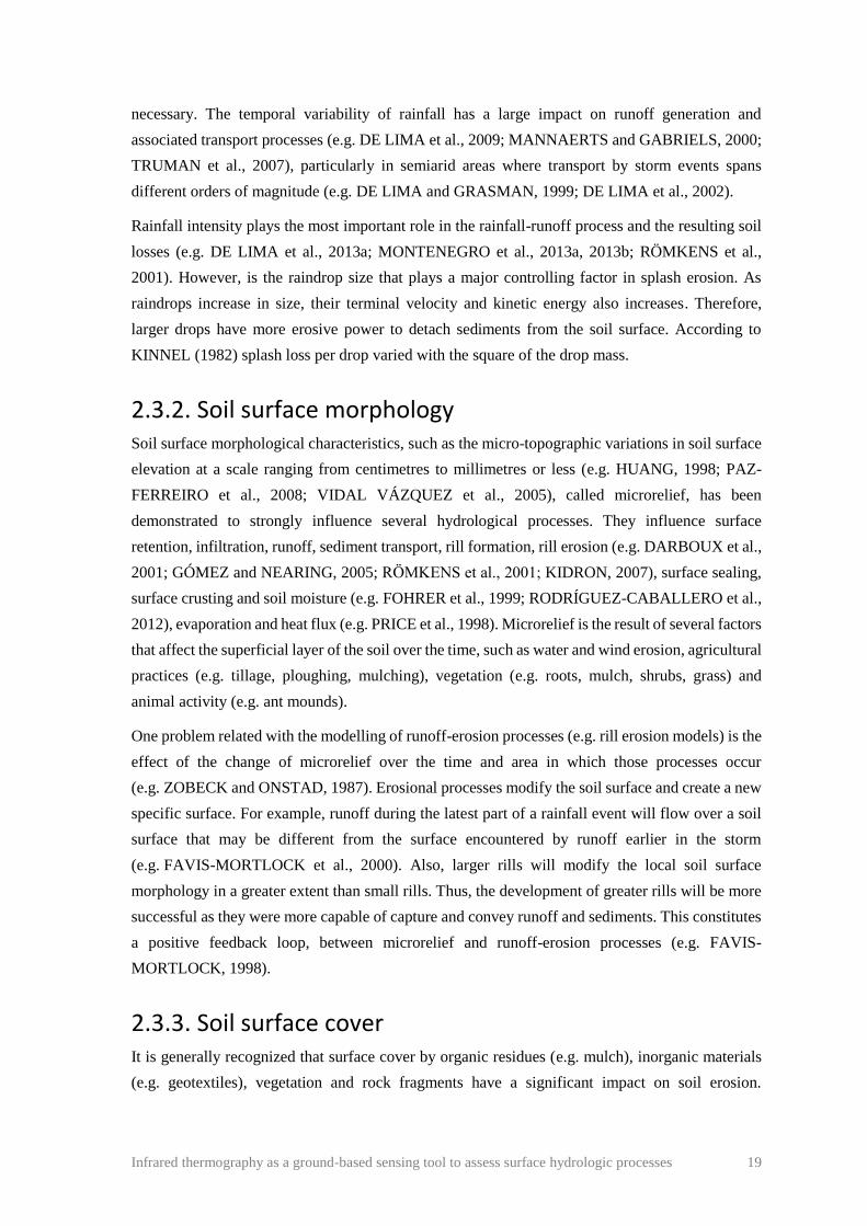
Infrared thermography as a ground-based sensing tool to assess surface hydrologic processes 19

necessary. The temporal variability of rainfall has a large impact on runoff generation and

associated transport processes (e.g. DE LIMA et al., 2009; MANNAERTS and GABRIELS, 2000;

TRUMAN et al., 2007), particularly in semiarid areas where transport by storm events spans

different orders of magnitude (e.g. DE LIMA and GRASMAN, 1999; DE LIMA et al., 2002).

Rainfall intensity plays the most important role in the rainfall-runoff process and the resulting soil

losses (e.g. DE LIMA et al., 2013a; MONTENEGRO et al., 2013a, 2013b; RÖMKENS et al.,

2001). However, is the raindrop size that plays a major controlling factor in splash erosion. As

raindrops increase in size, their terminal velocity and kinetic energy also increases. Therefore,

larger drops have more erosive power to detach sediments from the soil surface. According to

KINNEL (1982) splash loss per drop varied with the square of the drop mass.

2.3.2. Soil surface morphology Soil surface morphological characteristics, such as the micro-topographic variations in soil surface

elevation at a scale ranging from centimetres to millimetres or less (e.g. HUANG, 1998; PAZ-

FERREIRO et al., 2008; VIDAL VÁZQUEZ et al., 2005), called microrelief, has been

demonstrated to strongly influence several hydrological processes. They influence surface

retention, infiltration, runoff, sediment transport, rill formation, rill erosion (e.g. DARBOUX et al.,

2001; GÓMEZ and NEARING, 2005; RӦMKENS et al., 2001; KIDRON, 2007), surface sealing,

surface crusting and soil moisture (e.g. FOHRER et al., 1999; RODRÍGUEZ-CABALLERO et al.,

2012), evaporation and heat flux (e.g. PRICE et al., 1998). Microrelief is the result of several factors

that affect the superficial layer of the soil over the time, such as water and wind erosion, agricultural

practices (e.g. tillage, ploughing, mulching), vegetation (e.g. roots, mulch, shrubs, grass) and

animal activity (e.g. ant mounds).

One problem related with the modelling of runoff-erosion processes (e.g. rill erosion models) is the

effect of the change of microrelief over the time and area in which those processes occur

(e.g. ZOBECK and ONSTAD, 1987). Erosional processes modify the soil surface and create a new

specific surface. For example, runoff during the latest part of a rainfall event will flow over a soil

surface that may be different from the surface encountered by runoff earlier in the storm

(e.g. FAVIS-MORTLOCK et al., 2000). Also, larger rills will modify the local soil surface

morphology in a greater extent than small rills. Thus, the development of greater rills will be more

successful as they were more capable of capture and convey runoff and sediments. This constitutes

a positive feedback loop, between microrelief and runoff-erosion processes (e.g. FAVIS-

MORTLOCK, 1998).

2.3.3. Soil surface cover It is generally recognized that surface cover by organic residues (e.g. mulch), inorganic materials

(e.g. geotextiles), vegetation and rock fragments have a significant impact on soil erosion.

20 Infrared thermography as a ground-based sensing tool to assess surface hydrologic processes

GOVERS et al. (2006) reported that intensity of water erosion is strongly related to the presence

and density of rock fragments and vegetation (living plants and/or residues) on the soil.

Several investigations on the impact of mulching on runoff have been conducted, addressing the

effect of cover densities on surface flow, soil moisture, evapotranspiration and soil temperature

(e.g. COOK et al., 2006; MONTENEGRO et al., 2013a). JORDÁN et al. (2010) showed that long

term mulching application improved physical and chemical properties of a semiarid soil in Spain.

Increase in rainfall interception, delay in runoff generation, and reduction in runoff and sediment

yield were observed under mulching conditions. An important aspect highlighted by the authors

was the exhaustion of available erodible particles after storms longer than 30 minutes, thus reducing

sediment transport. In a laboratory study, MONTENEGRO et al. (2013a) applied a sequence of

intermittent rainfall patterns with different intensities and patterns, under the presence of different

mulch cover densities. They found that mulching dramatically reduced erosion rates, especially

during the rainfall events with higher intensity. Also, mulch increased infiltration and controlled

temperature fluctuations in soil. PRATS et al. (2015, 2017) observed that mulching 1/3, 2/3 and

3/3 of the flume’s length with forest residues at 70% ground cover, significantly reduced soil loss,

but not runoff. At 50% ground cover, only the application of mulch over the whole plot was able

to reduce soil loss significantly. Sieved forest residue mulch was less effective in reducing runoff

(10%) but more effective in reducing erosion (65%), as compared to the straw mulch (25 and 50%

runoff and soil loss reduction, respectively) in the study presented in ABRANTES et al. (2018b).

In these studies (ABRANTES et al., 2018b; PRATS et al., 2015, 2017) the authors observed that

mulching effectiveness decreased with water input. In a study by LOCH (2000), erosion from a

simulated storm was greatly reduced by vegetation cover, declining approximately 98% from 0 to

47% of vegetative covers. According to LI et al. (2008) the presence of vegetation cover resulted

in high infiltration rates, with unsaturated hydraulic conductivities significantly greater for the

vegetated surface than for the rock fragment covered surface and bare soil surface.

Rock fragment cover has ambiguous effects on overland flow and infiltration rates. While studying

the effect of rock fragments in the rain splash soil erosion, JOMAA et al. (2012) observed that the

presence of rock fragments protected the soil from raindrop splashes and from sealing, therefore

preserving the original soil structure and infiltration rate. However, this effect was conditioned by

the size and spatial distribution of the rock fragments. POESEN et al. (1999) found that surface

rock fragments are less efficient in decreasing concentrated flow erosion rates when the topsoil is

dry, than when the topsoil is wet. Surface rock fragments seemed to protect the underlying soil

more efficiently when it has been already wet for some time. According to LI et al. (2008) rock

fragments had no obvious effect on water infiltration and soil hydraulic conductivity as compared

with bare soils. In laboratory and field, PRATS et al. (2018) found that the presence of rocks, with

2 to 3 cm in size, on the top of the soil surface, significantly reduced soil loss. Surface runoff was

reduced but not significantly.

Infrared thermography as a ground-based sensing tool to assess surface hydrologic processes 21

2.3.4. Soil hydraulic characteristics Water movement on soil and the associated transport of fertilizers, pesticides and other pollutants

in the soil have significant impact on hydrological response and water quality (e.g. BEVEN et al.,

2006; KÖHNE et al., 2009; VAN DER HEIJDEN et al., 2013).

Permeability is the measure of the soil’s ability to allow water to flow through its pores or voids. It

depends not only on the pores but also to how they are connected and is affected, amongst other

factors, by land use, soil organisms, soil moisture and precipitation/irrigation. Permeability is one

of the most important soil property of interest to engineer’s purposes: i) Many hydrological models

require estimations of permeability to predict overland flow; ii) Changes in permeability can

provide an early warning of soil degradation, flood risk and erosion; and iii) Permeability is the key

factor for the design of subsurface drainage systems.

Macropores and water flow in soils and substrates are complex and related to topics like preferential

flow, non-equilibrium flow and dual-continuum, and have been the subject of many studies in the

last decades (e.g. the reviews by BEVEN and GERMANN, in 1982, and, most recently, 30 years

later, BEVEN and GERMANN, in 2013). Macropore is defined as a pore space which allows water

to move through the soil under gravity without being restrained by capillary tension (BEVEN and

GERMANN 1982) and can be formed by the cracking of the surface material or by biological

activity (e.g. ants, earthworms, burrowing mammals, roots). Some root systems, earthworm and ant

burrows extend for many metres below the surface and can have a significant effect on the

infiltration rate. Robert E. Horton was already aware of the effects of macropores on infiltration

(e.g. BEVEN, 2004). Since macropores affect soil permeability they directly influence other

hydrological processes (e.g. surface runoff and associated transport processes). Macropores convey

water to greater depths with higher speed, thus influencing water infiltration into the soil and solute

transport. According to VILLHOLTH (1998) in shallow unsaturated soils the effect of macropore

flow can be manifested through very short arrival times of surface-applied or derived substances to

the groundwater. Macropores also directly affect the flow of air into the soil, the root growth of

plants and biological activity (e.g. JARVIS, 2007; LUO et al., 2010; PERRET et al., 1999).

Therefore, a high macroporosity enhances air and water movement in the soil, promoting also

infiltration and root penetration.

Soil water repellency (also called soil hydrophobicity) is another characteristic of soil hydraulics

that affects different aspects of surface hydrology. Soil water repellency can alter infiltration and

water storage capacity of soils, enhancing infiltration by preferential flow and/or enhancing surface

runoff generation and associated erosion (KEIZER et al., 2005b; LEIGHTON-BOYCE et al., 2007;

RITSEMA and DEKKER, 1994; SHAKESBY et al., 1993; VIEIRA et al., 2014). Also, by altering

water availability SWR can indirectly affect seed germination, seed establishment and plant growth

(DOERR et al., 2000).

Repellent soils have been found in fire affected forest lands (BADÍA-VILLAS et al., 2014;

KEIZER et al., 2008; MATAIX-SOLERA and DOERR, 2004; SHAKESBY, 2011), but also in

22 Infrared thermography as a ground-based sensing tool to assess surface hydrologic processes

pine and eucalypt forest lands not affected by fires and in agricultural lands with high soil organic

matter content (DOERR et al., 2000, KEIZER et al., 2007, SANTOS et al., 2013). Other factors,

such as soil moisture (CHAU et al., 2014; FERREIRA et al., 2016; KEIZER et al., 2005a;

LEIGHTON-BOYCE et al., 2005), presence of fungi and bacteria species (SCHAUMANN et al.,

2007), soil texture and structure (URBANEK et al., 2007) and soil organic carbon content

(WIJEWARDANA et al., 2016) have shown to cause and/or influence soil water repellency.

However, its ultimate origin is the coating of soil particles with hydrophobic organic substances

usually released by plants or decomposing plant material (DEKKER and RITSEMA, 1994;

KEIZER et al., 2005c).

2.4. Measurement techniques in surface hydrology

2.4.1. Rainfall characteristics Many studies of rain have typically concentrated on its average properties over sufficiently large

volumes and time intervals, and not on characterizing the exact positions, sizes and fall speeds of

the individual raindrops. In such case, the stochastic and discrete nature of rainfall at smaller spatial

and temporal scales is usually treated only in a statistical sense. Some relatively recent

developments have contributed to the increased interest of the hydrological community in the

microstructure of rainfall and the attention devoted to understanding processes at the land surface,

such as soil detachment and erosion by raindrop impact, infiltration of rain water into the soil,

surface runoff and interception by vegetation canopies. In general, these are highly nonlinear

processes to which every raindrop can make a significant contribution. One example is the use of

weather radar for estimating the spatial and temporal distribution of rainfall (e.g. TETZLAFF and

UHLENBROOK, 2005).

Some examples of earlier proposed techniques that provide indirect estimation of the number and

size of the raindrops arriving at a surface during a particular sample interval, are: i) The flour

method (e.g. BENTLEY, 1904); ii) The blotter paper stain method (e.g. MAGARVEY, 1957); and

iii) The oil method (e.g. EIGEL and MOORE, 1983). PEARSON and MARTIN (1957) offer a

review of early attempts to assess the number, size and fall speed of raindrops, at the edge of

technological developments that have changed considerably the approaches used to obtain such

data. These latter measurement techniques will work well for sparse raindrops, not a heavy rain

(which will just spread all over the surfaces). Moreover, some of these simple techniques involve

quite time-consuming data processing; in addition, their accuracy and efficiency are limited

because they depend a lot on human measurement.

There have been some developments in relation to assessing raindrop properties. Examples of

devices and early studies that provide instantaneous measurements of the number and size of

raindrops, are the raindrop camera (e.g. JONES, 1992), the optical array probe

Infrared thermography as a ground-based sensing tool to assess surface hydrologic processes 23

(e.g. KNOLLENBERG, 1970), the electromechanical disdrometers (e.g. JOSS and

WALDVOGEL, 1969) and the optical spectrometers (e.g. BRADLEY and STOW, 1974). While

offering the possibility to acquire high resolution data and continuous records, some of the latter

techniques involve using expensive equipment and require the capability to handle and analyse

large data sets. The absence of required conditions makes it still necessary to consider the

possibility of using simplified methods to get insight into the drop size distribution.

2.4.2. Soil surface morphology An accurate modelling of surface hydrological processes requires detailed information on soil

surface microrelief and rill morphology with adequate resolution and precision (e.g. GOVERS et

al., 2007; KAMPHORST and DUVAL, 2001; KAMPHORST et al., 2000; LEI et al., 1998;

MANCILLA et al., 2005; NEARING, 1998; PLANCHON et al., 2001). A wide range of techniques

can be used to characterise and measure the soil surface microrelief and rill morphology (e.g. width,

depth) with an adequate resolution and precision for water erosion studies and modelling. Yet, this

is a task that may require a large consumption of time and/or resources (e.g. JESTER and KLIK,

2005). Measurement techniques can be classified as contact and noncontact and two-dimensional

(2D) and three-dimensional (3D).

The most common contact techniques, used to characterize soil surface roughness are profile or pin

meters (e.g. GILLEY and KOTTWITZ, 1995), chain and set methods (e.g. MERRILL et al., 2001)

and automatic relief meters (e.g. HANSEN et al., 1999). These techniques measure soil surface

roughness along a single profile. The main benefits of these techniques are the low cost and easy

handling. However, these techniques present limited resolution and may induce deformation to the

soil surface.

Nowadays, there are very accurate noncontact techniques that allow the generation of digital

elevation models with enough resolution for microrelief analysis, being the most commonly used

the laser techniques (e.g. DARBOUX and HUANG, 2003; EITEL et al., 2011) and the

photographic techniques like photogrammetry methods (e.g. RIEKE-ZAPP and NEARING, 2005;

WARNER, 1995) and shadow analyses (e.g. GARCIA MORENO et al., 2008, 2010). While laser

techniques consist mainly in 2D devices measuring roughness, photogrammetry is able to measure

soil surface roughness in 3D giving a more realistic value of the roughness measure. Other

noncontact techniques using ground based (e.g. SANKEY et al., 2011) and airborne (TURNER et

al., 2014) light detection and ranging devices (LiDAR) and acoustic backscatter devices (e.g.

OELZE et al., 2003; ZRIBI et al., 2014) have also been applied to characterize the surface

morphology.

One of the main problems when assessing information on soil surface microrelief for water erosion

studies is the presence of vegetation covering the soil surface (i.e. mulching). In fact, with high

vegetation covers microrelief cannot be estimated by these techniques, since you measure the mulch

characteristics instead of the soil surface bellow.

24 Infrared thermography as a ground-based sensing tool to assess surface hydrologic processes

2.4.3. Soil hydraulic characteristics Several experimental investigations have been carried out aiming to the development of

measurement techniques for estimating soil hydraulic characteristics (e.g. HAVERKAMP et al.,

2006; REYNOLDS and ELRICK, 1985; ŠIMŮNEK and HOPMANS, 2002; VEREECKEN et al.,

2007).

In general, small scale measurement techniques rely on precise and time-consuming experimental

procedures. In situ experimental measurements can be carried out in the field, based on small scale

infiltration tests under saturated or unsaturated soil conditions. Among these methods, the double-

ring infiltrometer, the Beerkan method developed by BRAUD et al. (2005) and the Guelph

Permeameter method, proposed by REYNOLDS and ELRICK (1985) have been largely adopted

(e.g. SILVA et al., 2012; XU et al., 2009). These methods can be conveniently applied to the field

conditions because of the simple experimental apparatus. However, e.g. the ring methods cannot

be used on a sloping soil surface. In such cases, experimental permeability measurements must be

obtained in the laboratory using disturbed or undisturbed soil samples. Since, permeability is highly

variable over different spatial scales, traditional permeability tests need to be grouped or scaled to

bring out spatial coherence (WANG et al., 2001) in order to properly represent distributed patterns

of variations and for distributed spatial analysis.

The development of simple cost-effective approaches for determining the occurrence of preferential

flow (e.g. through macropores) is required to identify risks of agrochemical mobilisation to

groundwater (e.g. HARDIE et al., 2013). A review of different approaches for identifying the

occurrence and extent of preferential flow through the soil is presented in ALLAIRE et al. (2009).

One approach identified by the author, is to use X-ray and magnetic resonance imaging (MRI) to

observe the soil structure and soil porosity. These techniques resulted in very good representations

of the network pore system with very high spatial resolution. However, these systems require staff

with very specific technical knowledge, are very expensive and are difficult to handle. Also, most

of the times, it is not possible to transport that equipment to the filed. Thus, requiring the transport

of samples to the scanning site (e.g. hospital), which, in general, is not feasible.

Other approach identified by ALLAIRE et al. (2009) is to use dye tracers. The dye tracer technique

(e.g. FLURY et al., 1994) consists in the application of a dye at the soil surface either with water

or before water infiltration, excavation of the soil profile after a specified infiltration time, analysis

of visual and/or photo interpretation of dye distribution with computer software. These approaches

are easy to apply, inexpensive and gives a range of macroporosity levels and other features causing

preferential flow. However, they are imprecise, the characteristics of the dye may affect

interpretation, are destructive and labour intensive. According to ALLAIRE et al. (2009) much

progress has recently been made in quantifying preferential flow in soil. In particular, dye tracing

with image analysis has significantly evolved in recent years so that dye concentrations from photos

can be quantified and even the type of interaction between macropores and the matrix can now be

evaluated.

Infrared thermography as a ground-based sensing tool to assess surface hydrologic processes 25

Regarding soil water repellency, the two most commonly used techniques to measure it are the

Molarity of an Ethanol Droplet (MED) test, also known as Percentage of Ethanol test or Critical

Surface Tension test (LETEY, 1969) and the Water Drop Penetration Time (WDPT) test

(VAN’TWOUDT, 1959).The MED test uses the surface tension of an ethanol solution to indirectly

measure the apparent surface tension of the soil surface, i.e. how strongly water is repelled. The

WDPT determines how long repellency persists in the contact area of a water drop. Both the MED

and WDPT tests provide quantitative data, but the subsequent classification or characterization of

these data vary with the objective of the investigator and perception of what constitutes low or high

repellency severity. Other techniques to measure soil water repellency include measurement of the

water-soil contact angle (LETEY et al., 1962), measurement of ethanol and water ethanol sorptivity

(TILLMAN et al., 1989), measurement of the water entry pressure head of a soil (CARRILLO et

al., 1999), and the sessile drop method using a goniometer-fitted microscope (BACHMANN et al.,

2000). Most of these techniques have been compared in various papers such as COSENTINO et al.

(2010), DEKKER et al. (2009), KING (1981) and LETEY et al. (2000).

An important problem in assessing the hydrological role of soil water repellency is that most of the

existing techniques to quantify soil water repellency require specialized equipment and are best

suited for use in the laboratory (DEKKER et al., 2009). Some of these techniques require air-dried

or oven-dried samples which may not be very representative of the conditions occurring in the field.

Also, some of these techniques (e.g. WDPT) can be very time consuming in the presence of strong

to extreme repellency. Other problem with most of the existing techniques is that they provide

punctual data, not revealing the spatial extent of the repellency severity. At field and landscape

scales, punctual measurements must be grouped or scaled to bring out spatial coherence, in order

to properly map soil water repellency and represent distributed patterns of variations. This presents

a laborious and time-consuming task.

2.4.4. Flow velocity Most research related to hydraulics and hydrology relies on the accurate measurements of flow

velocity. In particular, shallow flows that often occur in natural and urbanized drainage basins, have

important implications, such as water erosion and water quality. Flow velocity is a basic hydraulic

property of overland flow and its precise calculation is a necessary component of all process based

hydrological models such as soil erosion and rill development models (e.g. GIMÉNEZ et al., 2004;

GOVERS, 1992; WIRTZ et al., 2012), as well as in modelling sediment and solute transport by

runoff (e.g. LEI et al., 2010; MÜGLER et al., 2011).

Flow velocity measuring techniques vary with water body dimension, its accessibility and

characteristics. Recently, significant developments have been made in sensing technology,

resulting in a wide spectrum of powerful and versatile options for high accuracy flow velocity data.

However, measurement devices may have some limitations when operating outside their ideal

measurement conditions. Particularly for shallow flows, the characterization of the velocity fields

26 Infrared thermography as a ground-based sensing tool to assess surface hydrologic processes

is complicated, mostly because of their lack of depth (anything from several millimetres to a few

centimetres) and other problems, such as variability of the channel bed due to erosion, presence of

sediment and other debris in the flow or even the presence of vegetation concealing the measuring

area. This restricts the use of many flow measuring devices.

For deeper water bodies (e.g. large rivers) flow velocity can be measured with current meters or

acoustic Doppler techniques, such as acoustic Doppler velocimetry (ADV) or acoustic Doppler

current profiler (ADCP), at determined monitoring sections (e.g. KIMIAGHALAM et al., 2016;

MUSTE et al., 2004a, 2004b). Although intrusive, these techniques do provide a reliable

characterization of the flow velocity vertical profile; however, these instruments cannot always be

used in very shallow water. Other techniques, such as satellites, radars and microwave sensors,

hand-held or coupled in a drone, can be used to estimate surface flow velocity accurately and non-

intrusively (e.g. BJERKLIE, 2007; BJERKLIE et al., 2003; FULTON and OSTROWSKI, 2008);

however, these methods are usually very costly and satellite data are typically applied to large water

bodies.

For a long time, common techniques used in shallow flow velocity measurements for soil erosion

studies were based on the determination of the travel time of a tracer across a defined section, in

both laboratory (e.g. ABRAHAMS and ATKINSON, 1993; GIMÉNEZ and GOVERS, 2002) and

field conditions (e.g. HORTON et al., 1934; WIRTZ et al., 2012). In fact, many researchers regard

tracer methods as crude methods that yield a maximum flow velocity that must be corrected to give

a mean velocity. However, in shallow muddy flows, with depths of a few millimetres to a few

centimetres, it is not always possible to use the more sophisticated methods to measure true mean

flow velocity, such as ADV, ACDP. When using tracers, the accuracy of the measurement depends

to a great extent on the tracer added to the flow and on the quality of its detection in the flow.

According to FLURY and WAI (2003) an ideal tracer for hydro-environmental research should

have the following characteristics: i) Movement similar to water; ii) Be conservative, i.e. without

degradation during the measurement time; iii) Not show sorption to other environment components

(e.g. soil, sediments, rocks); iv) Be clearly distinguishable from the background of the system;

v) Be detectable either by chemical analysis or by visualization; and vi) Low toxicological impact

on the study environment.

Among the different materials that have been tested as tracers in flow velocity experiments are

natural and radioactive isotopes (NIAZI et al., 2017), floating objects (TAURO et al., 2012a),

fluorescent particles (TAURO et al., 2012a, 2012b, 2012c), bacteria (e.g. MAURICE et al., 2010),

salts (e.g. CALKINS and DUNNE, 1970; DAY, 1977; LEI et al., 2005, 2010; SHI et al., 2012) and

dyes (e.g. ABRAHAMS et al., 1986; DUNKERLEY, 2003; FLURY and FLÜHLER, 1993;

HOLDEN et al., 2008; TAZIOLI, 2011). Depending on the used tracer, optical cameras (e.g. for

dyes, floating objects), fluorometers (e.g. for fluorescent particles, fluorescent dyes) or electrical

conductivity sensors (e.g. for salt tracers), can be used. A review of tracer technology in hydrologic

studies is presented in LEIBUNDGUT et al. (2009).

Infrared thermography as a ground-based sensing tool to assess surface hydrologic processes 27

Optical methods for flow characterization, such as particle image velocimetry (PIV) and particle

tracking velocimetry (PTV), have seen great development and have been adjusted so that they can

be used in natural environments (e.g. COZ et al., 2010; KANTOUSH et al., 2011; TAURO et al.,

2014, 2016). These methods combine digital cameras and lasers to track the movement of particles

(tracers) dispersed in the water (e.g. fluorescent particles, air bubbles, floating objects) and thereby

better estimate the surface flow velocity. LEI et al. (2005) proposed an alternative methodology for

determining shallow flow velocities based on an advection-dispersion solute transport model. This

numerical technique consisted on fitting the analytical solution of the differential equation for

solute transport in shallow flows to solute transport data obtained by means of a salt tracer. This

fitting was done by minimising the sum of squared errors between modelled and experimentally

observed data. This method has been used in several studies involving the determination of shallow

flow velocity (BAN et al., 2016; CHEN et al., 2017; HUANG et al., 2018; LEI et al., 2010, 2013;

RAHMA et al., 2013; SHI et al., 2012, 2016; ZHUANG et al., 2018).

2.5. Infrared thermography

2.5.1. Background, operating principles and applications Infrared thermography is a technique with which it is possible to detect and measure the radiated

infrared (thermal) energy emitted from the surface of a given material. Infrared energy is the

electromagnetic radiation with wavelengths between 0.74 microns and 1000 microns, i.e. the zone

in the electromagnetic spectrum between the visible light and microwaves. Every object with

temperature above the absolute zero emits infrared energy and its emittance increases with

temperature. Since the human eye can only detect a narrow range of wavelengths, between 0.4 to

0.7 microns (visible wavelength), infrared thermographic systems must be used to detect and

measure the infrared radiation. These systems are mainly comprised of infrared cameras that use

special lenses to detect the infrared radiation in their field of view, which is converted to digital

signals. These signals are then processed and are converted to temperature values that are associated

to a colour scale and are displayed as a thermal image (i.e. group of pixels each one with a colour

associated to a temperature value) in a monitor associated to the camera or in a computer.

When using these systems, it is important to note that: i) Most common infrared cameras detect

radiation in the long-wavelength infrared (8μm-14μm), not the entire infrared spectrum (materials

in the temperature range from approximately -83 ºC to 726 ºC emit radiation in this spectral range);

ii) Human eye transparent materials (e.g. transparent glass, transparent acrylic) can be opaque in

the long-wavelength infrared, blocking the radiation emitted by the objects behind it; and iii) Two

materials with different emissivity (physical property of any material), at the same temperature,

may appear differently in the thermal image (the contrary can also happen, i.e. two materials with

different emissivity, at different temperatures, may appear equal in the thermal image).

28 Infrared thermography as a ground-based sensing tool to assess surface hydrologic processes

During the last decades, the development of thermographic systems has been rapidly growing.

According to GADE and MOESLUND (2014), although infrared light was discovered by William

Herschel around 1800, the first infrared scanning devices were only built in the late 1940s and

1950s, for the American military for the purpose of night vision. The first commercial products

were only produced in 1983 and opened up a large area of new applications. According to

ROGALSKI (2011), on the last 25 years array size has been increasing at an exponential rate, with

the number of pixels doubling every 19 months. Recently Teledyne Imaging Sensors developed an

infrared imaging sensor that combining a total of 35 arrays each with 2048 × 2048 pixels, producing

an image with 147 megapixels.

Thermography is a versatile technique and allows us to measure the spatial and temporal variability

of temperature in a non-invasive and a non-destructive way. Nowadays infrared thermography is

used in a variety of fields (BAGAVATHIAPPAN et al., 2013; GADE and MOESLUND, 2014):

i) In veterinary, to diagnose diseases, control reproductive processes, analyse animal behaviour,

detect and estimate population sizes; ii) In food production, to obtain information about the quality,

such as damage and bruises in fruits and vegetables; iii) In building inspection, to detect heat loss

from buildings (e.g. thermal bridges), to detect termites; iv) To detect an anomalous gas and track

to locate the source of the gas leak; v) In industry, as a diagnostic tool for electrical joints in power

transmission systems, to evaluate specific properties in different materials, detect malfunctions in

objects; vi) In motorized sports for dynamic analysis of the temperature of the tires during a race;

v) For fire detection in particular homes, industrial facilities and forests; vi) For military purposes,

to detect and locate the origin of a gunfire, detect mines, vi) In the surveillance and detection of

intruders; vii) For safety applications like the detection of fall accidents or unusual inactivity; vii) In

face recognition, to estimate anxiety levels, evaluate emotion of, drivers detection; viii) In

medicine, to breast cancer detection, diabetes neuropathy, fever screening, dental diagnosis, brain

imaging; and ix) In physical rehabilitation to monitor and interpret communications from people

with motor impairments.

For more information about the background history of infrared thermography, operating principles,

applications, types of sensors, composition of the lenses and other characteristics of the technology,

along with the recent developments observed in this field, see the reviews by

BAGAVATHIAPPAN et al. (2013), GADE and MOESLUND (2014) and ROGALSKI (2011).

2.5.2. Applications in surface hydrology Infrared thermography has been successfully employed as a high spatial and temporal resolution

non-intrusive imaging tool in surface hydrology. Some of the first hydrologic studies using infrared

thermography, rely on satellite data, and date back to the 1970's and 1980's, after the launch of the

first satellites equipped with infrared sensors. Infrared satellite imagery has been used to estimate

rainfall over large space and time scales (GRIFFITH et al., 1978), to assess evapotranspiration over

large agricultural regions (e.g. TACONET et al., 1986), to identify the potential of groundwater

Infrared thermography as a ground-based sensing tool to assess surface hydrologic processes 29

flow, that can provide valuable input to the hydrological modelling, the selection of sites for solid

waste disposal and non-point-source modelling (e.g. BOBBA et al., 1992). Satellite based infrared

systems have been used to characterize temperature patterns in oceans (e.g. EMERY and YU, 1997)

and lakes (e.g. HOOK et al., 2003).

Since the 1980’s, thermal sensing has been used and has been proved to be particularly useful for

the study of plant-water relations and to evaluate soil water deficit and crop water stress of several

agricultural and horticultural crops. A few examples are sunflowers (HASHIMOTO et al., 1984),

muskmelons (CLARKE 1997), grapevines (GRANT et al., 2007), soybean and cotton crops

(O'SHAUGHNESSY et al., 2011) and olive orchards (EGEA et al., 2017). URRESTARAZU

(2013) evaluate and determinate the capability of using infrared thermography as an early, rapid

and simple method for diagnosing salt tolerance or the salt stress level of a crop.

During the last decades, thanks to the technological development of high resolution, cost-effective

and robust handheld (i.e. portable) thermal imaging cameras, the use of infrared thermography

techniques in surface hydrology have undergone a significant increase. The increase in sensors

accuracy and spatial resolution, together with faster measurement and processing times and

improved quality of the thermographic data, allow hydrologists to rapidly image real-time

variations in temperature at high resolution in the field at scales from a few millimetres to several

meters. These studies can be carried at the air level by attaching the camera to an airborne vehicle

(e.g. drone) or at the ground level (e.g. hand-held, mounted on a tripod).

Differences between temperatures in a stream and surrounding sediments can be analysed to trace

the movement of groundwater to and from streams, and to better understand the magnitudes and

mechanisms of stream/groundwater exchanges (e.g. STONESTROM and CONSTANTZ, 2003).

DANIELESCU et al. (2009), KELLY et al. (2018) and MEJÍAS et al. (2012) used infrared cameras

mounted in aircrafts for mapping groundwater discharge in shallow estuaries and harbours,

provided that there is a thermal contrast between groundwater and the receiving surface waters.

Through handheld infrared data acquisition, CHEN et al. (2009) and SCHUETZ and WEILER

(2011) mapped and quantified localized groundwater inflow into streams.

Thermal infrared remote sensing has proven effective for mapping temperature heterogeneity of

streams and rivers (e.g. CARDENAS et al., 2008; TONOLLA et al., 2010). CARDENAS et al.

(2008) verified that remotely sensed stream temperatures acquired with handheld infrared camera

compared well with those measured with a digital thermometer. Thermal images shown a

significant spatial and temporal stream thermal variability. Such results have consequences for

thermally sensitive hydro-ecological processes and implications for their modelling. TONOLLA et

al. (2010) quantified the spatial and temporal thermal heterogeneity of entire river floodplains,

characterized aquatic and terrestrial floodplain habitat types, and quantified vertical temperature

patterns within unsaturated gravel sediment deposits. In this study, an infrared camera was mounted

on a tripod installed at the rim of steep mountains fringing on two floodplains, thereby allowing the

entire valley bottom to be thermally mapped.

30 Infrared thermography as a ground-based sensing tool to assess surface hydrologic processes

Climate change is altering river temperature regimes, modifying habitats temperatures and the

dynamics of temperature sensitive species. The ability to map river temperature is therefore

important for understanding the impacts of future warming (e.g. BAKER et al., 2019; DUGDALE

et al., 2019). DUGDALE et al., 2013 used an infrared camera mounted on a helicopter platform to

acquire thermal imagery of an Atlantic salmon river in Québec, Canada, with the objective of

characterize the temporal variability in thermal refuges and broader scale water temperature

complexity. According to BAKER et al. (2019), while ground-based infrared thermography can be

useful for qualitatively identifying stream temperature differences, acquisition of absolute stream

temperatures remains difficult due to interference from reflected radiation. In this study, analytical

and empirical methods were used to extract absolute stream temperatures from infrared imagery.

Since reflected temperatures and stream surface emissivity can be difficult to quantify, the

empirical correction approach offered the best alternative.

PFISTER et al. (2010) used ground-based thermal imagery as a simple, practical tool, for mapping

saturated area connectivity and dynamics. It was possible to discriminate between areas with snow

cover, snow melt, soil seepage and stream water. It was possible to detect when and where variably

saturated areas were active and when connectivity existed between the hillslope–riparian–stream

systems. According to PFISTER et al. (2010), this was a simple and inexpensive technology for

sequential mapping and characterisation of surface saturated areas and a useful complement to

conventional tracer techniques.

More recently, innovative infrared thermography techniques with specific methodologies have

been developed and tested to evaluate different hydraulic aspects of the soil (e.g. crust formations,

evaporative fluxes, rock porosity, permeability, macroporosity, soil water repellency). Generally,

these started with exploratory and proof of the concept studies performed under controlled

laboratory conditions, thus proposing a wide range of ideas for further scientific researches aiming

at implementing and validating these techniques, namely in real field conditions.

SOLIMAN et al. (2010) used infrared thermography to distinguishing soil surface crust formations.

Two samples of surface crust formed under different conditions and one sample of a bedrock soil,

with 6.0 × 4.5 × 2.5 cm3, were collected and used to evaluate the technique in laboratory. The

technique consisted in heating the samples for 420 min, using two 500 W halogen lamps, and in

recording the heating and later cooling with an infrared camera. Thermal inertia of the samples (i.e.

heating and cooling rates) showed to be directly proportional to density and inversely proportional

to porosity. Therefore, the two samples of surface crust presented higher thermal inertia. However,

no significant differences were observed between the two surface crust samples, despite the

differences in the formation process. The advantages this technique are: i) Minimum arrangements

and instrumentation (a heat input source and a suitable infrared camera); ii) Non-invasive nature

that requires minimum preparation of the samples and can estimate the thermal inertia from surface

measurements; and iii) Allow multiple comparisons of samples extracted from different

geomorphological units (e.g. comparing surface crusts formed in upstream and downstream of a

Infrared thermography as a ground-based sensing tool to assess surface hydrologic processes 31

dry valley), where variation of thermal inertia is linked to variation of depositional environments

and cementing processes. However, the technique requires large measurement time and it suits only

in dry and low moisture content samples. SHAHRAEENI and OR (2010, 2011) presented a new

method for the non-invasive determination of spatially and temporally resolved distributions of

evaporative fluxes from heterogeneous porous surfaces based on infrared thermography. High

resolution infrared imagery of evaporating surface temperature fields provides input to a surface

energy balance simplified solution to yield the evaporation rate spatial distribution. In laboratory

conditions, the authors studied evaporation patterns from surfaces of initially saturated sand

columns containing sharp vertical textural contrasts (fine‐sand inclusion in coarse‐sand

background) to evaluate the performance of the proposed method. Spatial and temporal infrared

thermal data were numerically inverted to obtain evaporation flux values that are compared with

rates of mass loss from direct weighing of the samples. MINEO and PAPPALARDO (2019),

presented an innovative potential laboratory test for the indirect estimation of porosity of intact

rock specimens. Their hypothesis was based on an existence of a relation between the cooling of

previously heated rocks and their porosity. After an initial heating phase, the cooling of the rocks

was monitored through infrared thermography. Results demonstrated that the cooling trend of rocks

within the first 10 min of test represented a reliable index for the indirect quantification of their

porosity.

Runoff initiation from raindrops falling onto an inclined planar impervious surface was investigated

in a laboratory experiment by NEZLOBIN et al. (2013). The authors used an infrared camera to

visualize different processes of runoff initiation, by applying simulated rainfall (water at a

temperature of approximately 18 ºC) over an inclined planar impervious surface (at a temperature

at around 23–24 ºC). The effect of the surface inclination on the runoff initiation process was

evaluated. Infrared thermography allowed visualizing drop cluster formation, clusters merging,

coalescence shrink and wetted trails at the surface.

One technique studied during this doctoral study was the estimation of raindrops size by means of

infrared thermography (DE LIMA et al., 2015a). Rain samples were collected on pre-heated acrylic

boards, which were exposed to rain during an instant, and thermograms were recorded. The area of

the thermal stains (i.e. signatures of the raindrops) emerging on the board was measured and

converted to drop diameters, applying a calibration equation. Diameters of natural raindrops,

estimated using this technique, were compared with laser disdrometer measurements. Results

confirmed the usefulness of this simple technique for sizing and counting raindrops, although it is

unsatisfactory in light rain or drizzle situations.

An innovative technique to estimate soil surface microrelief and rill morphology using infrared

thermography is presented in ABRANTES and DE LIMA (2014) and DE LIMA and ABRANTES

(2014a). The technique was tested in laboratory in a surface with artificially created rills and in a

surface eroded by flowing water, in bare soil conditions and in the presence of different mulch

densities. Heated water was used to create a temperature gradient on the soil surface and high-

32 Infrared thermography as a ground-based sensing tool to assess surface hydrologic processes

resolution soil surface thermal imaging were obtained using a portable infrared camera. The authors

were able to generate 3D models of soil surface elevation for both bare soil and soil covered with

organic residue. This technique is presented in Chapter 3 of this Thesis.

In DE LIMA et al. (2014b) a new technique to map soil surface permeability and to identify

preferential flow at the soil surface using infrared thermography is presented. The technique was

tested in a laboratory flume, where different scenarios were tested using soils with different

permeability. Heated water was applied to the soil surface and preferentially infiltrated and

penetrated the soil in the higher permeability areas which, consequently, presented higher

temperatures that could be recorded with an infrared video camera. This technique is presented in

Chapter 4 of this Thesis. Further tests were conducted in the field (data submitted for publication),

where infrared thermography was used for estimating the soil moisture and unsaturated hydraulic

conductivity of two distinct soils in the Mimoso representative catchment, located in the semiarid

region of Pernambuco state, Brazil. Based on the obtained data, it was possible to estimate the

unsaturated soil hydraulic conductivity of the two soils, relevant to the analysis of hydrological

processes, such as infiltration.

Infrared thermography was used to map soil surface macroporosity. This technique was first studied

in a laboratory soil flume (DE LIMA et al., 2014a). The technique consisted in applying heated

water to the soil surface and register the brief accumulation of water in macropores (artificially

created at the soil surface) with an infrared video camera. The technique allowed to estimate the

number, location and size of macropores with different sizes. This study is presented in Chapter 5

of this Thesis. The technique was further applied in the field on natural soil conditions in DE LIMA

et al. (2014c). Field tests were carried out in the campus of the Federal Rural University of

Pernambuco (UFRPE), Recife, Brazil; and in the Mimoso representative catchment, located in the

semiarid region of Pernambuco state, Brazil. The technique relied on heating the soil surface with

hot air for mapping soil surface macropores. In contrast to the hot water firstly used in the laboratory

(DE LIMA et al., 2014a), the hot air used in the field had no destructive impact on the soil.

A technique to map soil water repellency spatial variability using infrared thermography was also

developed. The technique was firstly tested in small-scale laboratory soil flume experiments, where

areas of the soil surface were artificially induced with repellency, and cold water was used to create

a temperature gradient on the soil surface (ABRANTES et al., 2017). A follow-up study in field

conditions with natural soil water repellency was conducted in a Pine (P. pinaster) and Eucalyptus

(E. globulus) forest site located in Pinhal de Marrocos, Coimbra, Portugal (ABRANTES et al.,

2016). These studies are presented in Chapters 6 and 7 of this Thesis.

Many authors have exploited the use of infrared cameras and thermal tracers to estimate flow

velocity (e.g. DE LIMA, 2013). SCHUETZ et al. (2012) used infrared thermal imaging combined

with the injection of heated water as an artificial tracer technique to characterize the spatial

distribution of flow paths and to assess transport properties in a 65 m2 experimentally constructed

wetland with water depths between 0.1-0.2 m. For the studied conditions the authors observed that

Infrared thermography as a ground-based sensing tool to assess surface hydrologic processes 33

heated water can be used as a conservative artificial tracer for plot scale experiments. LIANG et al.

(2012) studied the feasibility of using thermal imaging to investigate the scalar transport process in

shallow jet and wake flows with waters depths of 35 mm and 45 mm by adding warm water to the

flow. The authors found that the thermal imaging technique has great potential as a quantitative

flow visualisation technique for studying shallow turbulent dispersion characteristics. TAURO and

GRIMALDI (2017) applied PTV techniques to track the movement a thermal tracer deployed in a

natural stream, as a surface flow velocity measurement technique. Thermal videos were collected

with infrared camera and ice dices were used as tracer. Due to the meagre quantity of tracing

material and the simplicity of the experimental setup, the methodology showed to be promising and

advantageous against standard optical methods. Specifically, the combined use of thermal images

and PTV leads to reduced image pre-processing times and to accurate reconstruction of the surface

flow velocity field. Also, optical image-based methods are more severely affected by illumination

conditions and tracers’ visibility. On the other hand, some drawbacks of this methodology were the

practical handling of the ice dices, cost of thermal cameras, and higher degree of supervision in

applying PTV rather than algorithms based on high-speed cross-correlation. Under controlled

laboratory conditions, MUJTABA and DE LIMA (2018) tested the capability of cold oil droplets

as a new thermal particle tracer to measure the velocity of shallow overland flows (< 2 mm depth)

using an infrared-based PTV technique. Again, in this study, the authors stressed the potential of

using thermal imaging to estimate the velocity of shallow water bodies, because of the tracer's

conspicuous visibility and independence from illuminating conditions. LIN et al. (2019) tested

several thermal tracers, in both small natural streams and laboratory conditions, and developed a

proper tracking algorithm (i.e. PTV technique) to measure surface flow velocities. When applied

to imagery from a thermal camera, their tracking algorithm outperformed commonly used tracking

methods.

Part of the research developed in this doctoral study was dedicated to the development and

validation of thermal tracer techniques. Firstly, overland and rill flow velocities were estimated by

means of dye and thermal tracers and results of the two tracer techniques were compared (DE LIMA

and ABRANTES, 2014b). Secondly, a triple tracer experiment was conducted to compare the

thermal tracer technique with dye and salt tracer techniques under different hydraulic conditions,

namely bottom slope, bottom roughness and flow depth (ABRANTES et al., 2018a). Thirdly, an

analytical solution of an advection–dispersion transport equation was combined with thermal tracer

data to estimate shallow flow velocity (ABRANTES et al., 2019). These studies are presented in

Chapters 8, 9 and 10 of this Thesis. Field tests using thermal tracers were also carried out during

the doctoral study, and were presented in DE LIMA et al., 2015b. In the field, thermography was

particularly useful when dealing with very shallow water depths, where the current available

options have many limitations, often challenged by minimum working depths of equipment, or

other unfavourable conditions. The inexistence of constraints regarding the use of thermography in

the presence of sediments (muddy flows), debris or rocks is another advantage (usually also a

limitation for other methods).

“A rill in a barnyard and the Grand Canyon represent, in the main, stages of valley erosion

that began some millions of years apart.”

- George Gaylord Simpson

Infrared thermography as a ground-based sensing tool to assess surface hydrologic processes 37

3. CAN INFRARED THERMOGRAPHY BE USED TO ESTIMATE SOIL SURFACE MICRORELIEEF AND RILL MORPHOLOGY?1

3.1. Abstract

This study presents a new technique to estimate soil microrelief using infrared thermography. This

technique can be specifically useful to characterize soil surface microrelief, to identify preferential

flow paths in mulching conditions and to estimate soil surface elevation where other microrelief

measurement techniques cannot be successfully applied. Laboratory tests were carried out using

two soil flumes where different scenarios were tested: scenarios with artificial rills created at the

soil surface and scenarios with a surface eroded by flowing water. The technique was tested both

in bare soil conditions and in the presence of different mulching surface cover densities. Heated

water was used, and high-resolution soil surface thermal imaging was obtained using a portable

infrared video camera.

The proposed technique allows us to identify different microrelief structures at the soil surface and

to visualize preferential flow paths in mulching densities up to 4 t ha-1. Where other microrelief

measurement techniques cannot be used, the thermography allows obtaining 3D models of the soil

surface elevation, with satisfactory accuracy, knowing only 4 points of the soil surface. Higher

mulch cover densities (above 4 t ha-1) strongly affected the performance of the technique.

Keywords Soil microrelief; Measurement technique; Thermography; Rill visualization

3.2. Introduction

Microrelief is the spatial arrangement of the micro-topographic variations in soil surface elevation

at a scale ranging from centimetres to millimetres or less (e.g. HUANG, 1998; VIDAL VÁZQUEZ

et al., 2005; PAZ-FERREIRO et al., 2008). It is the result of several factors that affect the

superficial layer of the soil over the time, such as: water erosion (e.g. splash, interrill and rill

erosion), wind erosion, agricultural practices (e.g. tillage, ploughing, mulching), vegetation

(e.g. roots, mulch, shrubs, grass) and animal activity (e.g. ant mounds).

1 DE LIMA, J.L.M.P. and ABRANTES, J.R.C.B. (2014). Can infrared thermography be used to estimate soil

surface microrelief and rill morphology? CATENA, 113, 314-322. DOI:10.1016/j.catena.2013.08.011.

38 Infrared thermography as a ground-based sensing tool to assess surface hydrologic processes

Microrelief has been demonstrated to strongly influence several hydrological processes, such as

infiltration, runoff, sediment transport, rill formation, rill erosion (e.g. DARBOUX et al., 2001;

GÓMEZ and NEARING, 2005; KIDRON, 2007; RӦMKENS et al., 2001), surface sealing, surface

crusting and soil moisture (e.g. FOHRER et al., 1999; RODRÍGUEZ-CABALLERO et al., 2012),

evaporation and heat flux (e.g. PRICE et al., 1998). Most of the times, an accurate modelling of

those hydrological processes, especially the runoff-erosion processes (e.g. rill erosion), require

detailed information on soil surface microrelief and rill morphology with adequate resolution and

precision (e.g. GOVERS et al., 2007; KAMPHORST and DUVAL, 2001; KAMPHORST et al.,

2000; LEI et al., 1998; MANCILLA et al., 2005; NEARING, 1998; PLANCHON et al., 2001).

One problem related with the modelling of runoff-erosion processes (e.g. rill erosion models) is the

effect of the change of microrelief over the time and area in which those processes occur (e.g.

ZOBECK and ONSTAD, 1987). Erosional processes modify the soil surface and create a new

specific surface. For example, runoff during the latest part of a rainfall event will flow over a soil

surface that may be different from the surface encountered by runoff earlier in the storm (e.g.

FAVIS-MORTLOCK et al., 2000). Also, larger rills will modify the local micro-topography in a

greater extent than small rills. Thus, the development of greater rills will be more successful as they

were more capable of capture and convey runoff and sediments. This constitutes a positive feedback

loop, between microrelief and runoff-erosion processes (e.g. FAVIS-MORTLOCK, 1998).

A wide range of techniques can be used to characterise and measure the soil surface microrelief

and rill morphology (e.g. width, depth) with an adequate resolution and precision for water erosion

studies and modelling. Yet, this is a task that may require a large consumption of time and/or

resources (e.g. JESTER and KLIK, 2005). Measurement techniques can be classified according to

the sensing type as contact and noncontact techniques. The most common contact techniques, used

to characterize soil surface roughness, are profile or pin meters (e.g. GILLEY and KOTTWITZ,

1995), chain and set methods (e.g. MERRILL et al., 2001) and automatic relief meters (e.g.

HANSEN et al., 1999). The principal benefits of these techniques are the low cost and easy

handling. However, these techniques present limited resolution and may induce deformation to the

soil surface. Nowadays, there are very accurate noncontact techniques that allow the generation of

digital elevation models with enough resolution for microrelief analysis, being the most common

used: laser techniques (e.g. DARBOUX and HUANG, 2003; EITEL et al., 2011); and photographic

techniques like photogrammetry methods (e.g. RIEKE-ZAPP and NEARING, 2005; WARNER,

1995) and shadow analyses (GARCIA MORENO et al., 2008).

In agricultural and rural areas of arid and semiarid regions, water erosion is one of the most

important soil degradation processes (e.g. MARTINEZ-MENA, 2001; MAYOR et al., 2009;

CANTÓN et al., 2011). Runoff-erosion modelling is of great significance to improve soil and water

conservation management in those regions (HESSEL and TENGE, 2008). One of the main

problems when assessing information on soil surface microrelief for water erosion studies in

agricultural semiarid environments is the presence of vegetation covering the soil surface (i.e.

Infrared thermography as a ground-based sensing tool to assess surface hydrologic processes 39

mulching) that is one of the most used soil and water conservation method in those areas

(e.g. MONTENEGRO et al., 2013b; TOTIN et al., 2013). In fact, with high mulching covers

microrelief cannot be estimated by these techniques, since you measure the mulch characteristics

instead of the soil surface bellow.

This paper presents an innovative technique to estimate soil surface microrelief and rill morphology

using infrared thermography. Infrared thermography has been successfully applied as a high-

resolution imaging tool in hydrological studies: surface water temperature distributions

(e.g. DANIELESCU et al., 2009) and groundwater–surface water interaction (e.g. MEJÍAS et al.,

2012). In particular, studies carried with portable hand-held thermography systems have been

recently increasing, due to their easy handling and easy adjustment of measurement distance and

scale (e.g. CARDENAS et al., 2008; PFISTER et al., 2010; SCHUETZ et al., 2012).

The main goals of this study were: i) Verify if infrared thermography can be used to visualize

preferential flow paths and to identify microrelief elements (e.g. rills, depressions, mounds, ridges)

namely in the presence of mulch covering the soil surface; and ii) Try to generate a 3D model of

the soil surface, knowing only a few (at least two) points of the real topography. The technique

presented here pretends to be specifically useful when soil surface is covered with mulch, where

other microrelief measurement techniques cannot be successfully applied.

3.3. Methodology

3.3.1. Experimental setup A schematic representation of the experimental setup used in this study is shown in Figure 3.1. All

experiments presented here were conducted in laboratory.

Figure 3.1. Sketch of the setup used in the laboratory tests (not at scale).

40 Infrared thermography as a ground-based sensing tool to assess surface hydrologic processes

Soil flumes and soil characteristics The experiments were carried out using two rectangular free drainage soil flumes set at a 10%

slope: a narrower soil flume 0.3 m wide and a wider soil flume with a width of 1 m. Feeder boxes

were installed at the upslope end of each flume which allowed the application of a constant and

uniform flow of hot water to the soil surface of the flumes.

The sedimentary material used in the experiments consists of a sandy-loam soil and was collected

from the right bank of River Mondego (Coimbra, Portugal). Clear signs of water erosion (e.g. rills,

gullies) under natural rainfall were visible (DE LIMA et al., 2003). The soil presented 7% clay, 9%

silt and 84% sand and was mainly composed of quartz, feldspars, quartzite, muscovite and clay

minerals.

Both flumes and soil have been used in several research projects in the last years (e.g. DE LIMA

et al., 2003, 2011, 2013a; MONTENEGRO et al., 2013a).

Infrared video camera Soil surface and water temperatures (i.e. thermal videos and thermal imaging) were recorded with

an Optris PI-160 portable infrared video camera (Optris GmbH, Germany) with an optical

resolution of 160 × 120 pixels, a thermal resolution of 0.1 ºC, an accuracy of ±2%, a frame rate of

100 Hz and a lens with a field of view of 23° × 17° and focal length of 10 mm. The camera was

attached to a metal support structure over the soil surface with the focal length direction

perpendicular to the soil surface. The infrared camera can be moved in different directions, enabling

the study of different sections with different sizes.

The camera converts the invisible infrared energy emitted by the soil surface and water into a 2D

visual image. Because the imaging scale of the infrared camera is based on temperature emissivity

coefficients of the materials, it must be taken into account that, for the working spectral range of

the infrared camera (7.5-13.0 μm), water and soil emissivity coefficients are very similar and,

therefore, the associated errors could be ignored.

3.3.2. Soil surface microrelief scenarios Two study sections were defined at the surface of the flumes: i) A smaller section with

0.30 × 0.40 m2 at the narrower flume; and ii) A larger section with 0.75 × 1.00 m2 at the wider

flume. The study sections were defined 0.5 m downslope of the feeder boxes.

Different soil surface microrelief scenarios were tested on both study sections: scenarios with

artificial rills and scenarios on a surface eroded by flowing water where different mulch cover

densities were applied. Figure 3.2 shows photographs of the soil surfaces of the two flumes.

Infrared thermography as a ground-based sensing tool to assess surface hydrologic processes 41

Figure 3.2. Photographs of the soil surface of the flumes: a) Small study section with three small

artificially created rills; b) Small study section with three big artificially created rills; c) Bare soil

with microrelief created by water erosion; d) Low mulching cover; and e) High mulching cover.

X represents the distance along the width of the flumes and Y represents the distance along the

length of the flumes.

Scenarios with artificial rills Four scenarios with artificial rills were studied on the smaller section (narrower flume). The

artificial rills created at the soil surface had three different sizes (depth and width): i) Small rills

with 7 mm width and 7 mm deep; ii) Large rills with 12 mm width and 12 mm deep; and iii) Deep

rills with 7 mm width and 18 mm deep. Figure 3.3 presents the soil surface elevation profiles of the

four scenarios with artificial rills which were kept constant along the length of the study section.

Figure 3.3. Soil surface elevation profiles of the scenarios with artificial rills: a) Scenario with

three small rills (see Figure 3.2a); b) Scenario with three large rills (see Figure 3.2b); c) Scenario

with three deep rills; and d) Scenario with a combination of three rills with different sizes. X

represents the distance along the width of the flume and H represents the soil surface elevation.

42 Infrared thermography as a ground-based sensing tool to assess surface hydrologic processes

Scenarios on the surface eroded by water Six scenarios, with different mulching densities, were studied on the surface eroded by flowing

water created on the larger study section (wider flume): i) Bare soil (see Figure 3.2c); ii) Low

mulching cover with 0.5 t ha-1 density (see Figure 3.2d); iii) Medium low mulching cover with

1.0 t ha-1 density; iv) Medium mulching cover with 2.0 t ha-1; v) Medium high mulching cover with

4.0 t ha-1; and vi) High mulching cover with 8.0 t ha-1 density (see Figure 3.2e). Rice straw (Oryza

sativa L. ssp. japonica) was adopted as mulching.

3.3.3. Experimental procedure The air dried pre-sieved soil was manually spread along the flume and compacted, aiming to obtain

a bulk density of approximately 1700 kg m-3 (original soil bulk density). A sharp straight-edged

blade was used to produce a plane top surface. The soil was saturated and let to dry aiming to obtain

a desired consistency that allowed the creation of different reliefs at the soil surface, both artificially

and by water erosion. The artificial rills were created compressing rectangular wooden forms, of

known geometry and dimensions, against the soil surface. Microrelief created by water erosion was

obtained by applying a uniform water flux of approximately 500 ml s-1 over the soil surface, using

the feeder box installed upslope of the flume, during 30 min. The rice straw, previously air dried,

was applied uniformly along the study section trying not to disturb the soil surface microrelief.

The infrared thermography technique starts by applying to the soil surface, using the feeder boxes

located upslope of the flumes, water heated (e.g. in an electric kettle) to a temperature of

approximately 90ºC. Water was applied with the lowest possible discharge in order not to alter soil

surface microrelief. As the heated water flows along the study section, uniformly distributed, it

concentrates in the lower topographic elements (e.g. rills, surface depressions). Consequently, these

features should present higher temperatures. On the contrary, the higher topographic elements

(e.g. mounds) should present lower temperatures because the heated water does not concentrate

there. The thermal videos of the soil surface were monitored throughout the experiments in the

portable device. Three repetitions were conducted for each of the ten soil surface scenarios studied.

3.3.4. Data analyses The thermal videos obtained with the infrared camera were analysed with the objective of

identifying preferential flow paths and the existing microrelief elements on the soil surface

(e.g. rills, depressions, mounds, ridges). Thermograms of the soil surface (i.e. snapshots of the

thermal videos) were captured every second from the moment that the heated water reached the

upstream end of the study sections. The characteristics of the thermograms of the studied sections

(e.g. dimensions, number of pixels, pixel dimension) are shown in Table 3.1.

Infrared thermography as a ground-based sensing tool to assess surface hydrologic processes 43

Table 3.1. Characteristics of the thermal imaging obtained with the infrared camera for the two

studied sections.

Section Smaller Larger

Section dimension (m) 0.40 × 0.30 1.00 × 0.75

Optical resolution used (pixel) 144 × 108 160 × 120

Number of data points (pixel) 15552 19200

Pixel dimension (mm) 2.78 × 2.78 6.25 × 6.25

Temperature data extracted from the captured thermograms was converted into soil surface

elevation data, to generate 3D digital soil surface elevation models. The digital elevation models

were constructed by interpolation of the obtained data, using kringing method from Surfer 10

surface modelling program (Golden Software, Inc.).

Elevation data obtained with thermography was then compared with the real elevation data

measured with a manual profile meter, by means of statistical indexes and regression analyses. Real

elevation point data was measured at every 0.050 m and 0.001 m along the length and width of both

study sections. In the surface eroded by flowing water, real elevation measurements were taken

after the water erosion be induced. The surface remained almost the same during the experiments,

because after surface eroded by water be created it was left to rest, aiming to obtain a consistency

that allowed the application of the heated water without damage significantly the soil surface. Also,

heated water was applied with the lowest possible discharge in order not to alter soil surface

microrelief. For the experiments with the artificial rills, before each repetition of the experiments,

the soil surface microrelief and rills were created artificially with wooden forms. So, for each

scenario the microrelief was always the same.

Data conversion method The conversion method consists in transforming the temperature data of the thermograms into

elevation data using linear regressions comparing the real elevation of, at least, two points, chosen

from the soil surface with their corresponding temperatures extracted from the thermograms.

The conversion method was tested using five sets with different number points selected from the

soil surface: i) 2 points; ii) 4 points; iii) 6 points; iv) 8 points; and v) 10 points. Only the maximum

of 10 points were chosen because the aim of the technique is to be as simple as possible and

measuring soil surface elevation with precision is a laborious and time-consuming task. The points

were selected randomly. Only one restriction was defined on choosing the points: approximately

half of the points should be situated in lower microrelief elements (e.g. rills, depressions) and the

other half should be situated in higher microrelief elements (e.g. mounds, ridges). Five tests were

performed for each set of points, to ensure uniformity in the selection of points of the soil surface.

44 Infrared thermography as a ground-based sensing tool to assess surface hydrologic processes

Statistical indexes Random roughness (RR) is the index most commonly used in soil surface roughness and microrelief

studies (e.g. PLANCHON et al., 2001; RODRÍGUEZ-CABALLERO et al., 2012). ALLMARAS

et al. (1966) defined RR as the standard deviation (SD) of soil surface elevation after the slope and

tillage effects were removed, the upper and lower 10% of the measurements were eliminated and

with a log transformation of the raw data. However, in this study, RR was estimated simply as the

SD of soil surface elevation after the slope effect was removed, without removing the effect of the

rills, without the log transformation of the raw data (e.g. CURRENCY and LOVELY, 1970;

KAMPHORST et al., 2000) and without remove the upper and lower 10% of the measurements

(e.g. GARCIA MORENO et al., 2008; PAZ-FERREIRO, et al., 2008). RR was calculated using

Equation 3.1, for both measured values with the profile meter and obtained values with

thermography.

( )N

2

i

i 1

1RR H H

N =

= − (3.1)

where iH is the elevation value at data point i, and H is the average elevation data point and N is

the number of elevation data points. Minimum, maximum and average elevation values were also

calculated.

Regular regression and frequency analyses were also performed to estimate the accuracy of the

elevation data estimated with the technique presented in this study, comparing soil surface elevation

data measured with the manual profile meter and obtained with thermography. Goodness of fit was

evaluated based on the coefficient of correlation (r) and on the root mean square error (RMSE),

calculated as Equations 3.2 and 3.3.

( ) ( )( )

( ) ( )

N

i i

i 1

N N2 2

i i

i 1 i 1

Hobs Hobs Hsim Hsim

r

Hobs Hobs Hsim Hsim

=

= =

− −

=

− −

(3.2)

( )N

2i i

i 1

1RMSE Hobs Hsim

N =

= − (3.3)

where Hobsi is the observed (measured with the profile meter) elevation value at data point i, Hsimi

is the simulated (obtained with thermography) elevation value at data point i, Hobs is the average

observed elevation data point, Hsim is the average simulated elevation data point and N is the

number of elevation data points.

Infrared thermography as a ground-based sensing tool to assess surface hydrologic processes 45

3.4. Results and discussion

3.4.1. Scenarios with artificial rills Soil surface thermograms obtained for the scenarios with the artificially created rills are shown in

Figure 3.4. The visualization of these thermograms allows us to identify the rills at the soil surface,

perceptible by the vertical stripes with a lighter colour, which is the result of higher temperatures.

This happened because the heated water flowed into the rills, where it has concentrated. The points

at the top surface (i.e. points out of the rills) presented lower temperature, because the water in

these places has not concentrated as much as in the rills. Some thermograms presented points at the

top surface with a darker coloration (e.g. right side of Figure 3.4a and between the rills in

Figure 3.4d). This could be related to the dispersion of the water as it flowed along the study section.

In the thermograms it is also possible to identify some differences in the width of the rills: e.g. in

Figure 3.4b the rills with 12 mm thick present vertical stripes thicker than the rills with 7 mm thick

of Figure 3.4c. Beyond the distinction of the widths it is also perceptible the difference of the depth

between some rills: in Figure 3.4d the leftmost vertical stripe (rill with depth of 7 mm) presents a

darker coloration than the other vertical stripes (rills with 12 mm and 18 mm depth).

Figure 3.4. Thermograms of the soil surface with artificially created rills: a) Scenario with three

small rills; b) Scenario with three large rills; c) Scenario with three deep rills; and d) Scenario

with a combination of three rills with different sizes. X represents the distance along the width of

the study section, Y represents the distance along the length of the study section and T represents

the temperature of the soil surface.

Figure 3.5 presents a comparison between data measured with the manual profile meter and

obtained with the thermographic technique. The variation, in time, of the correlation between the

two types of data presented a similar trend in all the scenarios with artificial rills. As shown in

Figure 3.5a, the fit increased in the first 5 seconds and then remained approximately constant,

decreasing after, around, 20 seconds. That means that there is a considerable period of time when

it is possible to use the thermal imaging obtained, without loose too much accuracy.

46 Infrared thermography as a ground-based sensing tool to assess surface hydrologic processes

Figure 3.5. Comparison between soil surface elevation data measured with the manual profile

meter (obs) and obtained with thermography (sim), for the scenarios with rills created artificially

(see Table 3.2): a) Coefficient of correlation (r) over the time; b) Root mean square error (RMSE)

for the different number of points used to convert the temperature data; and c) Relative

differences of random roughness (RR), for the different number of points used to convert the

temperature data

Thermograms obtained 10 seconds after the water reached the upstream of the small study section

were chosen to test the performance of the thermographic technique. RMSE, RR and other

parameters presented in Table 3.2 were used to evaluate the effect of the use of different number

of points of the soil surface to transform the temperature data into elevation data. Both RMSE and

RR (Figures 3.5b and 3.5c) clearly indicate that at least 4 points of the soil surface should be used.

As more points were used the better of the performance of the technique. However, this

improvement is not meaningful, and it may not compensate the effort in measuring soil surface

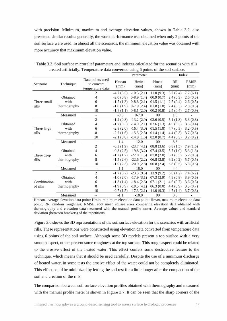
Infrared thermography as a ground-based sensing tool to assess surface hydrologic processes 47

with precision. Minimum, maximum and average elevation values, shown in Table 3.2, also

presented similar results: generally, the worst performance was obtained when only 2 points of the

soil surface were used. In almost all the scenarios, the minimum elevation value was obtained with

more accuracy that maximum elevation value.

Table 3.2. Soil surface microrelief parameters and indexes calculated for the scenarios with rills

created artificially. Temperature data converted using 6 points of the soil surface.

Parameter Index

Scenario Technique

Data points used

to convert

temperature data

Hmean

(mm)

Hmin

(mm)

Hmax

(mm)

RR

(mm)

RMSE

(mm)

Three small

rills

Obtained

with

thermography

2 -4.7 (6.5) -10.3 (2.1) 11.0 (9.3) 5.2 (2.4) 7.7 (6.1)

4 -2.0 (0.8) 0-8.9 (1.4) 00.9 (0.7) 2.4 (0.3) 2.6 (0.5)

6 -1.5 (1.3) 0-8.8 (2.1) 01.5 (1.1) 2.5 (0.4) 2.6 (0.5)

8 -1.0 (1.9) 0-7.9 (2.4) 01.8 (1.8) 2.4 (0.3) 2.8 (0.5)

10 -1.8 (1.1) 0-8.1 (2.0) 00.2 (0.8) 2.5 (0.4) 2.7 (0.9)

Measured - -0.5 0-7.0 00 1.8 -

Three large

rills

Obtained

with

thermography

2 -1.2 (0.8) -13.2 (2.9) 02.6 (0.5) 5.1 (1.8) 5.3 (0.8)

4 -1.7 (0.3) -14.9 (2.1) 02.6 (1.3) 4.5 (0.3) 3.5 (0.4)

6 -2.8 (2.0) -16.4 (3.0) 01.5 (1.8) 4.7 (0.5) 3.2 (0.8)

8 -2.7 (1.6) -15.5 (2.3) 01.4 (1.4) 4.4 (0.3) 3.7 (0.5)

10 -2.1 (0.8) -14.9 (1.6) 02.0 (0.7) 4.4 (0.3) 3.2 (0.2)

Measured - -1.4 -12.0 00 3.8 -

Three deep

rills

Obtained

with

thermography

2 -0.3 (1.9) -23.7 (4.1) 08.8 (3.6) 6.8 (1.5) 7.9 (1.6)

4 -0.3 (2.5) -19.8 (3.2) 07.4 (3.5) 5.7 (1.0) 5.3 (1.3)

6 -1.2 (1.7) -22.0 (1.5) 07.0 (2.0) 6.1 (0.3) 5.2 (0.3)

8 -1.5 (2.6) -22.6 (2.2) 06.8 (2.8) 6.2 (0.2) 5.7 (0.5)

10 -1.0 (2.3) -20.9 (2.8) 06.8 (2.4) 5.8 (0.5) 5.3 (0.5)

Measured - -1.1 -18.0 00 4.4 -

Combination

of rills

Obtained

with

thermography

2 -1.7 (6.7) -23.3 (9.5) 13.9 (9.2) 6.6 (4.2) 7.4 (6.2)

4 -1.0 (2.0) -17.9 (3.1) 07.3 (2.9) 4.5 (0.8) 3.9 (0.6)

6 -1.3 (1.4) -18.4 (2.6) 07.1 (2.1) 4.6 (0.7) 3.6 (0.5)

8 -1.9 (0.9) -18.5 (4.1) 06.3 (0.8) 4.4 (0.9) 3.5 (0.7)

10 -0.7 (1.5) -17.3 (2.1) 11.0 (9.3) 4.7 (1.4) 3.7 (0.3)

Measured - -1.1 -18.0 00 3.8 -

Hmean, average elevation data point; Hmin, minimum elevation data point; Hmax, maximum elevation data

point; RR, random roughness; RMSE, root mean square error comparing elevation data obtained with

thermography and elevation data measured with the manual profile meter. Average values and standard

deviation (between brackets) of the repetitions.

Figure 3.6 shows the 3D representations of the soil surface elevation for the scenarios with artificial

rills. These representations were constructed using elevation data converted from temperature data

using 6 points of the soil surface. Although some 3D models present a top surface with a very

smooth aspect, others present some roughness at the top surface. This rough aspect could be related

to the erosive effect of the heated water. This effect confers some destructive feature to the

technique, which means that it should be used carefully. Despite the use of a minimum discharge

of heated water, in some tests the erosive effect of the water could not be completely eliminated.

This effect could be minimized by letting the soil rest for a little longer after the compaction of the

soil and creation of the rills.

The comparison between soil surface elevation profiles obtained with thermography and measured

with the manual profile meter is shown in Figure 3.7. It can be seen that the sharp corners of the

48 Infrared thermography as a ground-based sensing tool to assess surface hydrologic processes

real topography are not well represented by the thermographic technique. This smoothing effect

could be caused by heat and turbulent diffusion.

Figure 3.6. 3D models of the soil surface elevation obtained by thermography for the scenarios

with rills created artificially: a) Scenario with three small rills; b) Scenario with three large rills;

c) Scenario with three deep rills; and d) Scenario with a combination of three rills with different

sizes. X represents the distance along the width of the study section, Y represents the distance

along the length of the study section and H represents the soil surface elevation.

Figure 3.7. Soil surface elevation profiles obtained with thermography and measured with the

manual profile meter, for the scenarios with artificial rills: a) Scenario with three small rills; b)

Scenario with three large rills; c) Scenario with three deep rills; and d) Scenario with combination

of three rills with different sizes. X represents the distance along the width of the study section

and H represents the soil surface elevation.

Infrared thermography as a ground-based sensing tool to assess surface hydrologic processes 49

3.4.2. Scenarios with surface eroded by water The application of the technique in a surface covered by mulch is presented in Figure 3.8.

Initially the soil was subjected to erosion by moving water; afterwards soil mulching covers with

different densities were applied. It can be seen that the presence of mulch affects the visualization

of water flow with the infrared camera, because straw conceals the paths of the water at the surface

of the soil. Also mulching creates a physical barrier to the flow altering the accumulation of water

at the soil surface and the preferential flow paths. However, below densities of 2 t ha-1 (medium

high mulching cover) it was still possible to identify satisfactory preferential flow paths and

distinguish different microrelief elements.

Figure 3.8. Thermograms of the surface eroded by water, for the scenarios with mulching cover:

a) Bare soil; b) Low mulching cover; c) Medium low mulching cover; d) Medium mulching

cover; e) Medium high mulching cover and f) High mulching cover. X represents the distance

along the width of the study section, Y represents the distance along the length of the study

section and T represents the temperature of the soil surface.

Higher mulching densities decreased the performance of the technique. Figure 3.9 shows a decrease

of the coefficient of correlation and an increase of the RMSE for increasing mulching cover

densities. For densities under 2 t ha-1 the performance of the technique was very similar. However,

the application of 4 t ha-1 strongly decrease the performance of the thermographic technique in

measuring soil surface elevation.

Relevant soil surface elevation data is presented in Table 3.3.

50 Infrared thermography as a ground-based sensing tool to assess surface hydrologic processes

Figure 3.9. Coefficient of correlation (r) and root mean square error (RMSE) comparing soil

surface elevation data measured with the manual profile meter and obtained with thermography,

for different mulching cover scenarios (see Figure 3.8). Thermograms used were obtained by

snapshots at 25 seconds.

Table 3.3. Soil surface microrelief parameters and indexes calculated for the mulching cover

scenarios. Temperature data converted using 6 points of the soil surface.

Parameter Index

Technique Mulching cover

density (t ha-1)

Hmean

(mm)

Hmin

(mm)

Hmax

(mm)

RR

(mm)

RMSE

(mm)

Obtained

with

thermography

0 -13.0 (1.2) -21.3 (2.5) -7.3 (1.7) 4.2 (1.0) 5.1 (0.3)

0,5 -11.6 (0.9) -20.3 (3.9) -6.5 (1.7) 3.9 (1.5) 5.2 (0.2)

1 -13.3 (0.9) -24.8 (4.4) -5.1 (2.9) 5.1 (1.8) 5.0 (0.6)

2 -13.5 (0.7) -28.0 (5.6) -3.5 (2.8) 5.3 (1.8) 5.3 (0.7)

4 -14.2 (1.6) -34.2 (6.5) -6.2 (3.1) 7.2 (1.4) 6.1 (0.7)

8 -15.8 (4.3) -54.7 (8.5) -5.3 (2.9) 8.1 (5.1) 9.3 (5.5)

Measured - -13.0 -30.4 -0.9 5.6 -

Hmean, average elevation data point; Hmin, minimum elevation data point; Hmax, maximum elevation

data point; RR, random roughness; RMSE, root mean square error comparing elevation data obtained with

thermography and elevation data measured with the manual profile meter. Average values and standard

deviation (between brackets) of the repetitions.

Figure 3.10 presents the 3D models of the soil surface elevation obtained with the thermographic

technique, converting data using 6 points of the real soil surface elevation.

As said before, the presence of higher mulching cover densities (i.e. 4 t ha-1 and above) affected the

performance of the studied technique. The cumulative empirical frequency distribution is strongly

affected by the presence of mulching, as it can be seen in Figure 3.11. For higher mulching densities

the empirical cumulative frequency distribution deviates from the measured surface elevation

distribution.

Infrared thermography as a ground-based sensing tool to assess surface hydrologic processes 51

Figure 3.10. 3D models of the soil surface elevation obtained by thermography of the scenarios

with surface eroded by water and mulching cover: a) Bare soil; b) Low mulching cover; c)

Medium low mulching cover; d) Medium mulching cover; e) Medium high mulching cover and f)

High mulching cover. X represents the distance along the width of the study section, Y represents

the distance along the length of the study section and H represents the soil surface elevation.

Figure 3.11. Cumulative frequency distribution of soil surface elevation data of the scenarios with

surface eroded by water, measured with the manual profile meter and obtained with

thermography for bare soil, low and high mulching cover densities. H represents the soil surface

elevation.

52 Infrared thermography as a ground-based sensing tool to assess surface hydrologic processes

3.5. Conclusion

This study presented a first approach to the use of an infrared thermography technique to estimate

soil surface microrelief and visualize preferential flow paths, namely in the presence of mulch

cover. It can be concluded that thermography:

• Can be used to visualize preferential flow paths and identify microrelief structures in the

presence of mulch covering the soil surface up to densities of 2 t ha-1 (valid for rice straw);

• Can be used to estimate soil surface microrelief and obtain 3D models of the soil surface

where other measurement techniques could not be applied.

The thermographic technique has shown to be of easy and fast application. The easy handling of

the equipment required, and low cost compared with other techniques make this technique to be

very usefully.

However, the following drawbacks can be appointed to the proposed thermographic technique:

• The precision of the technique in bare soil conditions was low compared with other

techniques available (e.g. laser scanning). This is especially true for sharp edges that tend to

be interpreted by this technique as being smoother;

• For high mulch cover densities (above 4 t ha-1) the measurements of the soil surface

temperatures are strongly affected;

• The technique can affect the soil surface microrelief (e.g. a second test will obtain a slightly

different soil surface microrelief), especially in easily erodible soils. It should be applied

carefully (e.g. use the lowest possible amount of heated water to avoid soil erosion).

“With reference to the expression ‘infiltration capacity’ I have found to my chagrin that there

are particularly in the Soil Conservation Service men who allege that they do not have

sufficient mental capacity to visualize the meaning of the word ‘capacity’ with but one of its

well accepted uses in physics and hydraulics, viz. as a volume. The Oxford English Dictionary

gives as the first definition of the word ‘capacity’: ‘ability to take in; ability to receive or

contain’. ... For the benefit of those having the limitations of mental capacity above suggested,

it may be well to point out that infiltration capacity is a volume per unit of time. A third

definition of ‘capacity’ given in the Oxford dictionary is ‘mental or intellectual receiving

power; ability to grasp or take in impressions, ideas, knowledge’. This is certainly something

more than the size of a man’s head.”

- Robert E. Horton

Infrared thermography as a ground-based sensing tool to assess surface hydrologic processes 55

4. PREDICTION OF SKIN SURFACE SOIL PERMEABILITY BY INFRARED THERMOGRAPHY: A SOIL FLUME EXPERIMENT2

4.1. Abstract

This study presents a new technique to map soil surface permeability using infrared thermography

and to identify preferential flow. Laboratory tests were carried out using a soil flume where

different scenarios were tested. Heated water was used to create a temperature gradient on the soil

surface and high-resolution soil surface thermal imaging were obtained using a portable infrared

camera. The technique was tested using soils with different permeability. The proposed technique

successfully allows us to identify different soil surface permeability and to visualize preferential

flows.

Keywords Thermography; Soil permeability; Preferential flow; Laboratory experiments; Soil flume

4.2. Introduction

Permeability is the measure of the soil’s ability to allow water to flow through its pores or voids. It

depends not only on the pores but also to how they are connected. Skin permeability is affected,

amongst other factors, by land use, soil organisms, soil moisture and precipitation/irrigation.

Permeability is probably the most important soil property of interest to engineer’s purposes. For

example: i) Many hydrological models require estimations of permeability to predict overland flow;

ii) Changes in permeability can provide an early warning of soil degradation, flood risk and erosion

(DIS4ME, 2013); and iii) Permeability is the key factor for the design of subsurface drainage

systems.

It is not possible to measure soil hydraulic properties everywhere by traditional methods. In general,

small scale measurement techniques rely on precise and time-consuming experimental procedures.

Several experimental investigations have been carried out over the last years aiming to the

development of measurement techniques for estimating soil hydraulic characteristics

2 DE LIMA, J.L.M.P., ABRANTES, J.R.C.B., SILVA JR., V.P. and MONTENEGRO, A.A.A. (2014).

Prediction of skin surface soil permeability by infrared thermography: a soil flume experiment. Quantitative

InfraRed Thermography Journal, 11(2), 161-169. DOI:10.1080/17686733.2014.945325.

56 Infrared thermography as a ground-based sensing tool to assess surface hydrologic processes

(e.g. REYNOLDS and ELRICK, 1985; ŠIMŮNEK and HOPMANS, 2002; HAVERKAMP et al.,

2006; VEREECKEN et al., 2007). In situ experimental measurements can be carried out in the

field, based on small scale infiltration tests under saturated or unsaturated soil conditions. Among

these methods, the double-ring infiltrometer, the Beerkan method developed by BRAUD et al.

(2005) and the Guelph Permeameter method, proposed by REYNOLDS and ELRICK (1985) have

been largely adopted (e.g. SILVA et al., 2012; XU et al., 2009). Large scale experiments (e.g.

pumping tests) cannot capture the spatial variability of permeability. Experimental permeability

measurements can also be obtained in the laboratory using disturbed or undisturbed soil samples.

Permeability is highly variable over different spatial scales, strongly influencing hydrological

processes. Hence, local scale traditional permeability tests need to be grouped or scaled to bring

out spatial coherence (WANG et al., 2001) in order to properly represent distributed patterns of

variations and for distributed spatial analysis.

Infrared thermography has been successfully applied as a high-resolution imaging tool in

hydrological studies: surface water temperature distributions and groundwater-surface water

interaction (e.g. DANIELESCU et al., 2009; MEJÍAS et al., 2012). Several recent studies have

appeared, carried out using portable hand-held thermography cameras due to their easy handling

and easy adjustment of measurement distance and scale (e.g. CARDENAS et al., 2008; DE LIMA

and ABRANTES, 2014a, 2014b; PFISTER et al., 2010; SCHUETZ et al., 2012).

The main goals of this study were: i) Verify if infrared thermography can be used to map areas of

lower and higher skin surface soil permeability; and ii) Verify if infrared thermography can be used

to identify preferential infiltration fluxes at the soil surface. This study follows several articles that

also made use of soil flumes in a controlled laboratory environment (e.g. DE LIMA and

ABRANTES, 2014a, 2014b; DE LIMA et al., 2003, 2011; MONTENEGRO et al., 2013a), some

of which have already used infrared thermography (DE LIMA and ABRANTES, 2014a, 2014b).

4.3. Materials and methods

4.3.1. Setup A schematic representation of the experimental setup used in the study presented here is shown in

Figure 4.1. The experiments were carried out using a 3.00 m long, 0.30 m wide and 0.12 m deep

free drainage soil flume set at a 10% slope. A feeder box was installed at the upslope end of the

flume which allowed the application of a volume of hot water uniformly to the soil surface.

The characteristics of the three substrates used in the experiments are presented in Table 4.1,

including saturated hydraulic conductivity (soil permeability) and bulk density.

Skin soil surface temperature distributions (e.g. thermal images) were recorded with a portable

infrared camera PI160 (Optris GmbH) with an optical resolution of 160 × 120 pixels, a thermal

resolution of 0.1 ºC, an accuracy of ±2%, and a frame rate of 100 Hz. The camera was positioned

Infrared thermography as a ground-based sensing tool to assess surface hydrologic processes 57

over the soil surface with the focal length direction perpendicular to the soil surface. A section of

the flume with 0.50 × 0.30 m2 was defined approximately 0.5 m of the hot water feeder box. The

section was surveyed by the infrared video camera.

Four different scenarios were tested: three scenarios with only two substrates (Soil_1 and Soil_2)

and one scenario with the three substrates (Soil_1, Soil_2 and Soil_3). Figure 4.2 shows sketches

of the soil surfaces of the flume for the different scenarios studied.

Figure 4.1. Sketch of the setup used in the laboratory tests (not at scale).

Table 4.1. Characteristics of the three substrates used in the laboratory experiments.

Material Brief characterization Saturated hydraulic

conductivity (m s-1)**

Bulk density

(kg m-3) Origin

Soil_1

Loamy sand soil (substrate)

presenting 4% silt, 11%

clay and 82% sand*

4.33 × 10-6 1750 Collected from the

left bank of River

Mondego

(Coimbra,

Portugal). Soil_2 Sieved sand 4.23 × 10-4 1500

Soil_3 Mixture of 50% Soil_1 and

50% Soil_2 1.75 × 10-5 1650

Mixed in the

laboratory

* Dry sieving for particles larger than 0.25 mm and wet sieving for particles finer than 0.25 mm; ** Data

obtained by using a constant head permeameter (30 mm layer of water over a 90 mm soil layer)

4.3.2. Experimental procedure The air dried substrates were manually placed along the flume and compacted in order to obtain

the different geometric shapes visualized in Figure 4.2, with the bulk densities shown in

Table 4.1.Thin (0.10 mm) flexible plastic film was used to create the different geometric shapes

and to separate the different substrates used avoiding mixing. A sharp straight-edged blade was

used to produce a plane top surface.

The technique starts by applying to the soil surface, using the feeder box located upslope of the

flume, approximately 1.5 L of heated water at a temperature between 80-85 ºC. Water was applied

with the lowest possible discharge in order not to alter soil surface configuration. The volume of

58 Infrared thermography as a ground-based sensing tool to assess surface hydrologic processes

applied water and discharge depend on the different characteristics of the soil (e.g. soil

permeability) and measurement section (e.g. area, shape).

Figure 4.2. Photographs of the soil surface of the flumes for the four scenarios tested. The

different soil can be distinguished by the different brightness. X represents the distance along the

length of the flume and Y represents the distance along the width of the flume. Dimensions in

metres.

As the heated water flows along the flume, uniformly distributed, part of the water infiltrates to the

soil and part flows freely out of the flume through the downslope outlet, as overland flow. The

heated water preferentially infiltrates and penetrates the soil in the higher permeability areas which,

consequently, will present higher temperatures. The more heated water infiltrates the soil the higher

will be the increase of temperature at the surface.

Thermal snapshots of the soil surface were taken just after overland flow has stopped

(approximately 30 s).

4.3.3. Data analyses The thermal videos obtained with the infrared camera were analysed with the objective of

identifying preferential flow and spatial differences in soil surface permeability. For each scenario,

the temperature data was converted into permeability data to generate soil surface permeability

maps. The conversion method consists in transforming the temperature data of the thermograms

into permeability data using linear regressions comparing the permeability of different points of the

soil surface with their corresponding temperatures extracted from the thermograms. Three points

for each substrate used were selected to convert the data. Permeability data (always positive)

obtained with the infrared thermographic technique were compared with the measured values

Infrared thermography as a ground-based sensing tool to assess surface hydrologic processes 59

obtained with a constant head permeameter (e.g. ELRICK and REYNOLDS, 1992; STOLTE,

1997), by means of statistical indexes and regression analyses.

Goodness of fit of soil surface permeability data was evaluated based on the coefficient of

correlation (r) and on the root mean square error (RMSE), calculated as (Equations 4.1 and 4.2):

( ) ( )( )

( ) ( )

N

i i

i 1

N N2 2

i i

i 1 i 1

Hobs Hobs Hsim Hsim

r

Hobs Hobs Hsim Hsim

=

= =

− −

=

− −

(4.1)

( )N

2i i

i 1

1RMSE Hobs Hsim

N =

= − (4.2)

where Hobsi is the observed permeability value (measured with constant-head hydraulic

conductivity test with permeameter) at data point i, Hsimi is the simulated permeability value

(obtained with thermography) at data point i, Hobs and Hsim are the average measured or

simulated permeability and N is the number of data points.

4.4. Results and interpretation

Thermograms of the four scenarios tested are presented in Figure 4.3. In the thermograms it is

clearly perceptible the delimitation of the areas with different permeability. The visualization of

thermograms allows us to identify the areas with higher permeability at the soil surface, perceptible

by the lighter colouration, which is the result of higher temperatures. This happened because more

heated water flowed into the soil in the higher permeability areas. Areas of lower surface

permeability presented lower temperature, because less water has infiltrated in these places.

Despite the soil in the eight circle areas of the scenarios A and D presented the same high

permeability (Soil_2), they have shown different surface temperatures. Infrared thermography

cannot adequately represent the smaller areas of high permeability. Also, small differences in

permeability are not easily detected, as shown in scenario D with Soil_1 and Soil_3.

Figure 4.4 presents a 3D representation of the permeability data obtained with the infrared

thermography. The technique enables the characterization of the spatial distribution of the soil

surface permeability.

Comparison between soil surface permeability obtained with thermography and measured with the

constant head permeameter (e.g. ELRICK and REYNOLDS, 1992; STOLTE, 1997), along cross

section lines, is shown in Figure 4.5. It can be seen that the sharp variation of permeability,

artificially created on the soil flume, were not well represented by the thermography technique.

This smoothing effect could be caused by higher diffusion of heat in those areas.

60 Infrared thermography as a ground-based sensing tool to assess surface hydrologic processes

Figure 4.3. Thermograms of the soil surface for the four scenarios tested. X represents the

distance along the length of the flume, Y represents the distance along the width of the flume and

T represents the temperature of the soil surface recorded with the infrared video camera.

Figure 4.4. 3D view of the soil surface permeability obtained with thermography for the scenarios

tested.

The technique is more efficient when characterizing larger high permeability areas. When areas of

different sizes, with the same permeability, are presented the technique tended to slightly

overestimate the permeability of larger areas and greatly underestimate permeability of smaller

areas. This is clearly visible in graphs of the cross sections A.1 and A.2 of scenario A and cross

sections D.1 and D.2 of scenario D.

Infrared thermography as a ground-based sensing tool to assess surface hydrologic processes 61

Figure 4.5. Comparison between soil surface permeability measured with the constant head

permeameter (blue straight lines) and obtained with thermography (red curved lines), along

longitudinal, transversal and oblique cross sections.

Coefficient of correlation (r) and root mean square error (RMSE) for the different scenarios are

presented in Table 4.2. The success of the technique in representing the soil surface permeability

of Scenarios B and C is shown by the high coefficient of correlation (r) of almost 1 and the lower

values of error (RMSE).

Table 4.2. Goodness of fit of soil surface permeability data obtained with thermography.

Scenarios Number of points Coefficient of correlation, r (-) Root mean square error, RMSE (m s-1)

A 9375 0.82 8.0 × 10-5

B 9375 0.90 7.9 × 10-5

C 9375 0.86 6.3 × 10-5

D 9375 0.85 7.0 × 10-5

62 Infrared thermography as a ground-based sensing tool to assess surface hydrologic processes

Scenarios A and D, which presented circular high permeability areas (Soil_2) of different sizes

presented lower values of r (approximately 0.5) and the higher values of RMSE. This is a

consequence of the difficulty of the technique in represent, at the same time, areas with very distinct

sizes (smaller circles with 7 mm radius and larger circles with 42 mm radius).

4.5. Conclusions

This technique can be specifically useful to identify preferential flow and to map areas of lower

and higher surface permeability in a expedite way. It can be concluded that infrared thermography:

• Can be used to visualize preferential flow;

• Can be used to estimate the spatial variability of soil surface permeability;

• Can be used to map approximate surface permeability spatial variation.

The thermographic technique has shown to be of easy and fast application. The easy handling of

the equipment required, and the small time spent compared with other techniques make this low-

cost procedure very interesting and promising.

The following drawbacks of the proposed thermographic technique should however be appointed

out:

• The precision of the technique has to rely on reliable measurements of permeability (in situ

or laboratory);

• Sharp variations of permeability tend to be interpreted by this technique as being smoother;

• The technique can affect the soil surface characteristics (e.g. a second test will obtain a

slightly different soil surface permeability map), especially in easily erodible soils, where

sediment transport can alter surface composition, or a surface crust can be formed.

In field application it is expected to allow the identification of areas with similar permeability,

therefore reducing the number of in situ random soil permeability tests (e.g. using double ring

infiltrometer), which are time consuming techniques. Future work has to be carried out to verify

the applicability of the proposed technique under different conditions, especially in field studies:

Test the influence of different soil surface conditions (e.g. soil surface roughness, initial soil

moisture content) and the presence of vegetation and other obstructions to the overland flow;

Test the technique at different scales, by increasing the measurement area (flooding area), and

observe how the technique is affected due to the need of higher amounts of heated water and loss

of uniformity of the flow.

“Engineers like to solve problems. If there are no problems handily available, they will create

their own problems.”

- Scott Adams

Infrared thermography as a ground-based sensing tool to assess surface hydrologic processes 65

5. MAPPING SOIL SURFACE MACROPORES USING INFRARED THERMOGRAPHY: AN EXPLORATORY LABORATORY STUDY3

5.1. Abstract

Macropores and water flow in soils and substrates are complex and are related to topics like

preferential flow, nonequilibrium flow, and dual continuum. Hence, the quantification of the

number of macropores and the determination of their geometry are expected to provide a better

understanding on the effects of pores on the soil’s physical and hydraulic properties. This

exploratory study aimed at evaluating the potential of using infrared thermography for mapping

macroporosity at the soil surface and estimating the number and size of such macropores. The

presented technique was applied to a small-scale study (laboratory soil flume).

Keywords Thermography; Soil surface macropores; Laboratory experiments; Soil flume

5.2. Introduction

Macropores and water flow in soils and substrates are complex, are related to topics like preferential

flow, nonequilibrium flow, and dual-continuum, and have been addressed by many studies in the

last decades, e.g. the reviews by BEVEN and GERMANN (1982) and, most recently, 30 years later,

BEVEN and GERMANN (2013). Since macropores affect soil permeability, they directly influence

other hydrological processes (e.g. surface runoff and associated transport processes).

The water movement and the fertilizers, pesticides, and other pollutants transporting in the soil

through macropores have significant impact on hydrological response and water quality

(e.g. BEVEN et al., 2006). These structures convey water to greater depths with higher speed, thus

influencing water infiltration into the soil and solute transport. The macropores also directly affect

the air flow into the soil, the plants root growth, and biological activity (e.g. JARVIS, 2007; LUO

et al., 2010; PERRET et al., 1999). Therefore, a high macroporosity enhances air and water

movement in the soil, promoting also infiltration and root penetration.

3 DE LIMA, J.L.M.P., ABRANTES, J.R.C.B., SILVA JR., V.P., DE LIMA, M.I.P. and MONTENEGRO,

A.A.A. (2014). Mapping soil surface macropores using infrared thermography: an exploratory laboratory

study. The Scientific World Journal, 2014, Article ID 84560. DOI:10.1155/2014/845460.

66 Infrared thermography as a ground-based sensing tool to assess surface hydrologic processes

Recently, infrared thermography has been successfully applied as a tool for high resolution imaging

in different hydrological studies, conducted at quite different spatial scales. Thermographic

techniques are based on records of bodies’ temperatures, which are taken at certain instants or over

time and at a given space scale; this technology is allowing for a nonconventional acquisition of

data and analysis of different processes and their time and space dynamics.

The use of portable infrared cameras or thermal imaging cameras has gained popularity due to their

easy handling and adjustment of the vision field to a specific study area. DANIELESCU et al.

(2009) and MEJÍAS et al. (2012) used infrared cameras mounted in aircrafts for mapping

groundwater discharge in shallow estuaries, provided that there is a thermal contrast between

groundwater and the receiving surface waters. CARDENAS et al. (2008) characterized the thermal

heterogeneity in a small stream during different flow conditions. PFISTER et al. (2010) used

ground-based thermal imagery as a simple, practical tool, for mapping saturated area connectivity

and dynamics. It was possible to discriminate between areas with snow cover, snow melt, soil

seepage, and stream water. It was possible to detect when and where variably saturated areas were

active and when connectivity existed between the hillslope-riparian-stream systems. This was a

simple and inexpensive technology for sequential mapping and characterisation of surface saturated

areas and a useful complement to conventional tracer techniques. SCHUETZ et al. (2012) used

infrared thermal imaging combined with the injection of heated water as an artificial tracer

technique to characterize the spatial distribution of flow paths and to assess transport properties in

a 65 m2 experimentally constructed wetland with water depths between 0.1 and 0.2 m. For the

studied conditions, the authors observed that heated water can be used as a conservative artificial

tracer for plot scale experiments.

Infrared thermographic techniques studied in laboratory conditions were used to assess different

surface hydrological processes. A technique to estimate soil surface microrelief and rill morphology

using infrared thermography is presented in DE LIMA and ABRANTES (2014a). The authors were

able to generate 3D models of soil surface elevation for both bare soil and soil covered with organic

residue. In DE LIMA and ABRANTES (2014b) the authors estimated very shallow flow velocities

(overland and rill flow), by injecting a thermal tracer (e.g. heated water) into very shallow flows

and visualizing the leading edge of the tracer by means of infrared video. Soil flume laboratory

experiments have been conducted for many years aiming at studying specific processes and

interactions in controlled conditions allowing for repetitions in a short period of time (e.g. DE

LIMA et al., 2003, 2005, 2011, 2013a; MONTENEGRO et al., 2013a, 2013b).

In situ small scale infiltration tests (e.g. profile or plot scale), under saturated or unsaturated soil

conditions, normally have difficulty to cope with macropores. The quantification of the number of

macropores, which are drivers of water, and the determination of their geometry will provide a

better understanding of the effects of pores on the physical and hydraulic properties of the soil

(e.g. SORACCO et al., 2012). Thus, this exploratory study aimed at evaluating the potential of

using infrared thermography for mapping macroporosity at the soil surface and estimating the

Infrared thermography as a ground-based sensing tool to assess surface hydrologic processes 67

number and size of such macropores. The presented technique was applied to a small laboratory

scale study (i.e. soil flume). Thus, upscaling results to field, hillslope, and even plot scales will

require further investigation, which is beyond the scope of the presented analysis.

5.3. Materials and methods

5.3.1. Laboratory setup A schematic representation of the used exploratory laboratory setup is shown in Figure 5.1. The

experiments were carried out using a 3.00 m long, 0.30 m wide, and 0.12 m deep free drainage soil

flume, set at a 10% slope (round number also used in many other works). A feeder box installed at

the upslope end of the flume allowed the application of a defined volume of hot water uniformly

over the soil surface. A rectangular measuring area (0.50 × 0.30 m2) with macropores was defined

at the flume soil surface, approximately 0.5 m downstream of the hot water feeder box.

Figure 5.1. Sketch of the laboratory setup using a soil flume and an infrared video camera.

The experiments were carried out using a loamy-sand soil collected from the River Mondego banks

(Coimbra, Portugal). The soil presented 6% clay, 11% silt, 82% sand, and a 1750 kg m-3 bulk

density. Saturated hydraulic conductivity was 4.51 × 10−6 m s-1, for the macropores-free soil.

Thermal videos of the soil surface were recorded with an Optris PI-160 portable infrared video

camera (Optris GmbH, Germany) with an optical resolution of 160 × 120 pixels, a thermal

resolution of 0.1 °C, an accuracy of ±2%, a frame rate of 100 Hz, and a lens with a view field of

23º × 27º and focal length of 10 mm. The camera was attached to a metal support structure 0.75 m

hot water

feeder box

soil surface

soil flume at

10% slope

infrared video camera

scanned surface area

(0.5×0.3 m2)

outlet

surface flow direction

surface flow

excess

free drainage

portable

monitor

outlet acrilic

protection

macropores

68 Infrared thermography as a ground-based sensing tool to assess surface hydrologic processes

above the flume soil surface with the focal length direction perpendicular to the soil surface

(Figure 5.1).

5.3.2. Soil surface macropores Soil surface vertical macropores with three different rectangular cross section areas were artificially

created to test the proposed thermographic technique: i) Large macropores with an area of 256 mm2

(16 × 16 mm2); ii) Medium macropores with an area of 120 mm2 (12 × 10 mm2); and iii) Small

macropores with an area of 36 mm2 (6 × 6 mm2). The tests were conducted for four different

macropores spatial arrangement’s scenarios; these scenarios are shown in Figures 5.2: a) 9 large

macropores (Scenario A); b) 9 medium macropores (Scenario B); c) 9 small macropores (Scenario

C); and d) a combination of 3 large, 3 medium, and 3 small macropores (Scenario D). It should be

noted that field conditions are quite different from a uniform plane surface, clean of stones, debris,

and vegetation, with homogeneous colours and macropores with well-defined shapes, used in this

exploratory study.

Figure 5.2. Top view (photographs) of the flume soil surface showing macropores of different

sizes scattered in accordance to the four scenarios described in the text: a) Scenario A; b)

Scenario B; c) Scenario C; and d) Scenario D. The x axis represents the downslope distance along

the length of the flume and the y axis represents the distance across the width of the flume (the

dashed line defines the measuring area with 0.50 × 0.30 m2). See Figure 5.1.

x

y

x

y

x

y

x

y

(a) (b)

Scenario A Scenario B

(d)

Scenario D

(c)

Scenario C

Surface flow direction

Scanned surface area

Infrared thermography as a ground-based sensing tool to assess surface hydrologic processes 69

5.3.3. Experimental procedure Air dried pre-sieved soil was manually spread over the flume and gently tapped to obtain a soil

layer with a uniform thickness of 0.10 m with a bulk density of 1750 kg m-3. A sharp straight-edged

blade was used to produce a smooth plane soil surface. The soil was saturated and left to dry, aiming

to obtain a consistency that allowed the artificial creation of vertical macropores at the soil surface;

this was carried out by perforating the soil layer, throughout its 0.10 m thickness, with rectangular

cross-section metal rods that were described in section 5.3.2. After the creation of the macropores,

the soil was again saturated.

The technique starts by applying approximately 1.5 L of heated water over the soil surface, at a

temperature around 80-85 °C. The water was manually released using the feeder box located

upslope of the flume (Figure 5.1). It was applied with the lowest possible discharge in order to

guarantee flow depth uniformity over the measuring area, minimum soil surface disturbance, and

the unaltered structure of the macropores by the flowing water. The volume of hot water used (and

applied discharge) should be adjusted to the test’s conditions (e.g. dimension of the measuring area,

slope, water temperature, soil permeability, and dimension of macropores).

The hot water created a wave that covered uniformly the soil surface; along the flume, part of the

water flows to the macropores, part infiltrates into the soil, and part flows out of the flume through

the downslope outlet, as overland flow. The hot water briefly accumulates inside the macropores

before exiting freely the soil layer due to the flume free drainage (Figure 5.1). Since macropores

were filled with flowing hot water, they present higher temperatures in the thermal videos, recorded

with the infrared video camera, which allowed the mapping of their spatial location and the

estimation of their approximate area. Because the soil was close to the field capacity at the

beginning of the experiments, the percentage of water infiltrated into the soil was very low

compared to the percentage flowing into the macropores.

Soil surface thermal videos were recorded with the infrared camera throughout the experiments.

However, thermograms of the surface of the overland flow layer did not provide any spatial

variability of temperature. therefore, for each scenario (Figure 5.2), a thermogram of the soil surface

was selected, corresponding to an instant just after (approximately 30 s) the passage of the wave of

hot water through the scanned area; thermogram is a graphic record of temperature variations, and

represent radiation in the infrared range of the electromagnetic spectrum, providing identification

of pixels associated with different surface temperatures. Because, in general, macropores present

higher temperatures, a threshold temperature (τ) can be selected that allows identifying the pixels

associated with the macropores (i.e. pixels with temperature values above a given threshold

temperature), thus distinguishing them from the remaining pixels that cover the soil surface scanned

area (i.e. pixels with temperature values below the temperature threshold). The percentage of pixels

that have temperature above the threshold temperature was called threshold percentage of pixels

(α).

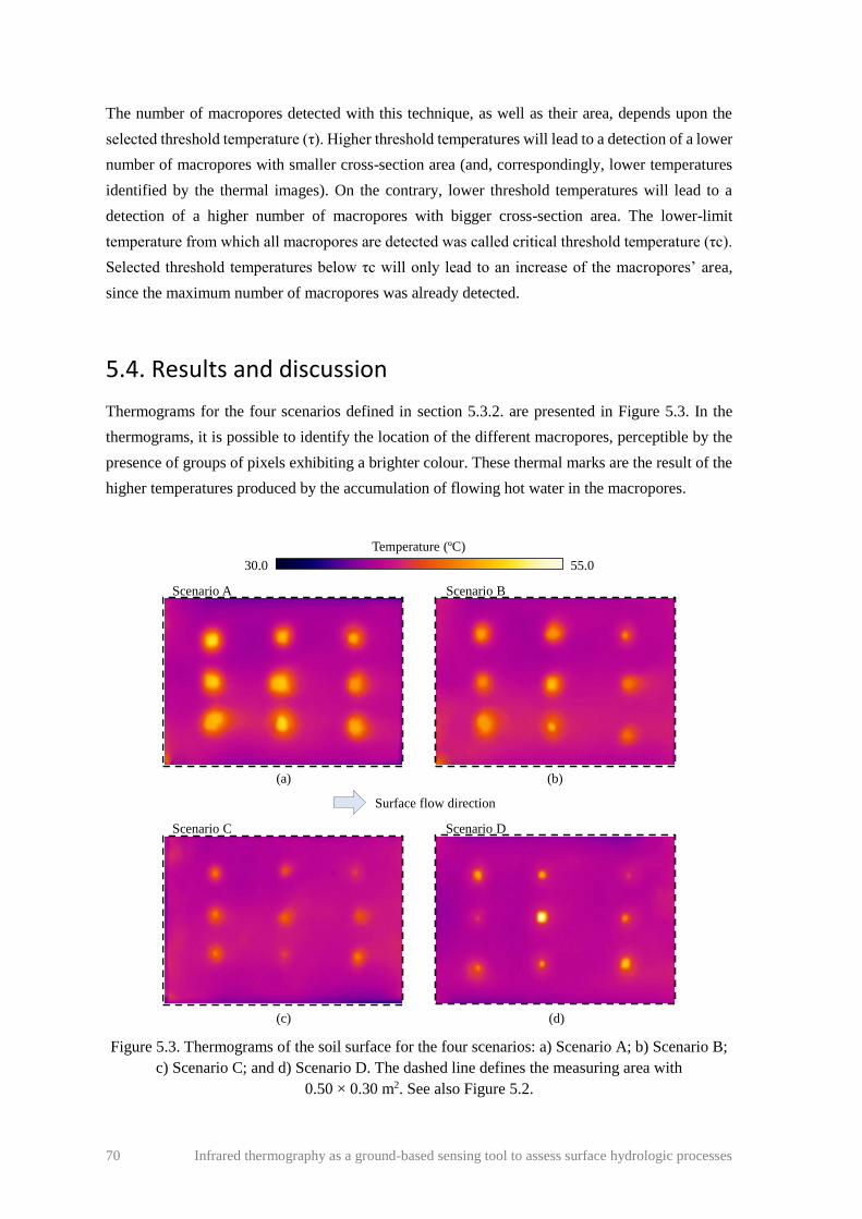
70 Infrared thermography as a ground-based sensing tool to assess surface hydrologic processes

The number of macropores detected with this technique, as well as their area, depends upon the

selected threshold temperature (τ). Higher threshold temperatures will lead to a detection of a lower

number of macropores with smaller cross-section area (and, correspondingly, lower temperatures

identified by the thermal images). On the contrary, lower threshold temperatures will lead to a

detection of a higher number of macropores with bigger cross-section area. The lower-limit

temperature from which all macropores are detected was called critical threshold temperature (τc).

Selected threshold temperatures below τc will only lead to an increase of the macropores’ area,

since the maximum number of macropores was already detected.

5.4. Results and discussion

Thermograms for the four scenarios defined in section 5.3.2. are presented in Figure 5.3. In the

thermograms, it is possible to identify the location of the different macropores, perceptible by the

presence of groups of pixels exhibiting a brighter colour. These thermal marks are the result of the

higher temperatures produced by the accumulation of flowing hot water in the macropores.

Figure 5.3. Thermograms of the soil surface for the four scenarios: a) Scenario A; b) Scenario B;

c) Scenario C; and d) Scenario D. The dashed line defines the measuring area with

0.50 × 0.30 m2. See also Figure 5.2.

30.0 55.0

Temperature (ºC)

(a) (b)

Scenario A Scenario B

(d)

Scenario D

(c)

Scenario C

Surface flow direction

Infrared thermography as a ground-based sensing tool to assess surface hydrologic processes 71

Despite the rectangular shape of the macropores, the thermal marks identified visually in the

thermograms are of approximate circular shapes. Also, the thermal marks are, in general, larger

than the actual area of the macropores. This temperature smearing around the macropores is caused

by thermal diffusion, by the higher infiltration of hot water around the macropores, and by the

relatively low resolution of the camera.

In general, larger macropores led to larger thermal marks, exhibiting higher temperatures at the

centre. Thermograms of Scenarios A, B and C, of Figures 5.3a to 5.3c, clearly show thermal marks

with different areas, which are in accordance to the different areas of the macropores of each

scenario. In the thermogram of Scenario D, in Figure 5.3d, it is also possible to distinguish the

macropores of different areas in the same thermogram. Macropores concentrate water which flows

into these hollows and are, therefore, in contact with more hot water. This is why macropores have

a different temperature than the surrounding soil.

The relation between the threshold temperature (τ) and the number of macropores detected with

thermography is shown in Figure 5.4 (right axis). The same graph shows the temperature

cumulative frequency distribution of the pixels’ temperature (T), corresponding to the four

thermograms in Figure 5.3, curve up to 2.5% (left axis).

For each scenario, the critical threshold temperature (τc) and corresponding critical threshold

percentage of pixels (αc) are identified in the figure. We highlight that both τc and αc depend on

the area of the thermal marks in the thermograms: e.g. Scenario A, with only large macropores,

leads to the highest τc and αc. The threshold τc depends also on the temperature of the hot water

applied, the initial surface temperature and the macropores present at the soil surface. Therefore, is

not possible to specify single τc or αc values, representative of all scenarios. Nevertheless, such

values are essential for processing the data and mapping existing soil surface macropores.

Therefore, bearing in mind the results obtained in our experiment for all the tests (Figure 5.4), we

have further adopted a threshold percentage of pixels (α) of 2.5% for all scenarios, since in our tests

we found always αc < 2.5%. For each scenario, the corresponding temperature frequency

distribution curve (Figure 5.4) yields a specific value of the threshold temperature (τ) for α = 2.5%,

which we have used to study the area and location of the macropores, using thermography.

Soil surface macropores were identified by applying to the temperature data the threshold

temperature (τ) corresponding to α = 2.5%; the selected τ were subtracted to all temperature values

from the thermograms: positive values, which correspond to pixels with temperature values above

τ, are associated to the macropores.

72 Infrared thermography as a ground-based sensing tool to assess surface hydrologic processes

Figure 5.4. Relation between threshold temperature (τ) and the number of macropores detected

with thermography, for the four scenarios: a) Scenario A; b) Scenario B; c) Scenario C; and d)

Scenario D. Temperature cumulative frequency distribution curves are also plotted, up to 2.5%.

Critical threshold temperature (τc) and corresponding critical threshold percentage of pixels (αc)

are also identified.

The comparison between the boundaries of the actual macropores and the macropores’ area

detected with thermography is shown in Figure 5.5. The macropores’ area detected with

thermography was, in general, larger than their actual area. Therefore, the technique did not

accurately estimate the actual area of the macropores, especially for the smaller ones. It is possible

to observe in Figure 5.5d that the proposed technique can be used to distinguish macropores with

different size (i.e. cross-section area), since larger macropores were detected with thermography as

having also larger areas. This has already been suggested by observing the thermal marks in the

thermograms in Figure 5.3 and the photographs in Figure 5.2.

Figure 5.6 shows the comparison between the position of the actual geometric centre of the

macropores and their geometric centre detected using thermography. In general, the proposed

technique allowed the correct estimation of the macropores’ location. Although, the technique did

not assess accurately the actual area of macropores, it clearly allowed mapping the macropores and

identifying their spatial distribution and position across the studied soil surface area.

35 40 45 50 55

Threshold temperature, (ºC)

0123456789

Num

ber

of

mac

ropore

s

det

ecte

d w

ith t

her

mo

grp

hy

0

0.5

1

1.5

2

2.5

Tem

per

atu

re c

um

ula

tive

freq

uen

cy d

istr

ibuit

ion (

%)

35 40 45 50 55

Threshold temperature, (ºC)

0123456789

Num

ber

of

mac

ropore

s

det

ecte

d w

ith t

her

mogrp

hy

0

0.5

1

1.5

2

2.5

Tem

per

ature

cu

mula

tiv

e

freq

uen

cy d

istr

ibuit

ion (

%)

35 40 45 50 55

Threshold temperature, (ºC)

0123456789

Num

ber

of

mac

ropore

s

det

ecte

d w

ith t

her

mogra

phy

0

0.5

1

1.5

2

2.5

Tem

per

ature

cum

ula

tive

freq

uen

cy d

istr

ibuit

ion (

%)

35 40 45 50 55

Threshold temperature, (ºC)

0123456789

Num

ber

of

mac

ropore

s

det

ecte

d w

ith t

her

mogrp

hy

0

0.5

1

1.5

2

2.5T

emper

ature

cu

mula

tiv

e

freq

uen

cy d

istr

ibuit

ion (

%)

(a)

τc = 47.0ºC

αc = 2.30%

Scenario A

(c)

τc = 39.5 ºC

αc = 1.55%

Scenario C

(b)

τc = 42.9 ºC

αc = 1.90%

Scenario B

(d)

τc = 40.0 ºC

αc = 1.25%

Scenario D

Number of macropores

detected by thermography

Temperature cumulative

frequency distribuition

Infrared thermography as a ground-based sensing tool to assess surface hydrologic processes 73

Figure 5.5. Comparison between the boundaries of the actual macropores and the area detected

with thermography, for the four scenarios. Across the area scanned by the thermographic camera,

the macropores are located using (x,y) coordinates: The x axis represents the downslope distance

along the length of the flume (0.5 m) and the y axis represents the distance across the width of the

flume (0.3 m). See also Figures 5.2 and 5.3.

Figure 5.6. Comparison between the actual geometric centre of the macropores and their

geometric centre detected using thermography, for four scenarios. See Figure 5.5.

0 0.1 0.2 0.3 0.4 0.5

x (m)

0

0.1

0.2

0.3

y (

m)

0 0.1 0.2 0.3 0.4 0.5

x (m)

0

0.1

0.2

0.3

y (

m)

0 0.1 0.2 0.3 0.4 0.5

x (m)

0

0.1

0.2

0.3

y (

m)

0 0.1 0.2 0.3 0.4 0.5

x (m)

0

0.1

0.2

0.3

y (

m)

Actual bounderies of

macropores

Area of macropores detected

with thermography

(a)

Scenario A

α = 2.5% τ = 46.7 ºC

(b)

Scenario B

α = 2.5% τ = 42.0 ºC

(c)

Scenario C

α = 2.5% τ = 38.5 ºC

(d)

Scenario D

α = 2.5% τ = 38.1 ºC

0 0.1 0.2 0.3 0.4 0.5

x (m)

0

0.1

0.2

0.3

y (

m)

0 0.1 0.2 0.3 0.4 0.5

x (m)

0

0.1

0.2

0.3

y (

m)

0 0.1 0.2 0.3 0.4 0.5

x (m)

0

0.1

0.2

0.3

y (

m)

0 0.1 0.2 0.3 0.4 0.5

x (m)

0

0.1

0.2

0.3

y (

m)

(a)

Scenario A

α = 2.5% τ = 48.1 ºC

(b)

Scenario B

α = 2.5% τ = 45.9 ºC

(c)

Scenario C

α = 2.5% τ = 41.9 ºC

(d)

Scenario D

α = 2.5% τ = 42.6 ºC

Actual geometric

centre of macropores

Geometric centre of macropores

detected with thermography

74 Infrared thermography as a ground-based sensing tool to assess surface hydrologic processes

5.5. Conclusions

A novel technique to detect and characterize soil surface macropores based on infrared

thermography was presented and discussed, based on exploratory laboratory soil flume

experiments. For our laboratory conditions, the thermographic technique was successful in

identifying the presence of macropores at the soil surface, providing a low cost and fast

methodology to map soil surface macropores. Although uncertainties arise during the analysis

about the macropores boundaries at the soil surface, which therefore restricts the quantification of

their shape and size, the technique seems promising and able to identify macropores’ spatial

distribution with satisfactory accuracy.

Only extensive field work can, in fact, reveal the relevance of the technique in real (field)

conditions. Future work has to be carried out to verify the applicability of the proposed technique

under different field conditions, such as e.g. soil type, dimensions of scanned area, surface

microrelief and roughness, presence of vegetation, stones and other obstructions, which is beyond

the scope of the presented analysis.

“Start by doing what's necessary; then do what's possible; and suddenly you are doing the

impossible.”

- Unknown

Infrared thermography as a ground-based sensing tool to assess surface hydrologic processes 77

6. ASSESSING SOIL WATER REPELLENCY SPATIAL VARIABILITY USING A THERMOGRAPHIC TECHNIQUE: AN EXPLORATORY STUDY USING A SMALL-SCALE LABORATORY SOIL FLUME4

6.1. Abstract

This exploratory study presents a technique to assess soil water repellency (SWR) spatial variability

based on infrared thermography. Small-scale laboratory tests were carried out using a soil flume

and a loamy-sand soil, where SWR was induced on soil surface with waterproofing spray and

repellent areas were mapped through thermal imaging, using a portable infrared video camera. Cold

water was used to create a temperature gradient on the soil surface in order to assess SWR.

The technique was, in overall terms, successful in mapping SWR spatial variability, distinguishing

repellent from wettable areas as well as distinguishing between areas with different levels of SWR

severity, in particular, between areas with extreme as opposed to low to medium SWR. The

proposed technique apparently has high potential to contribute to a better understanding of the

hydrological impacts of different spatial patterns of SWR due to its capacity to monitor in real time

the dynamics of these impacts.

Keywords Soil water repellency; Infrared thermography; Spatial variability; Laboratory soil flume

experiments

6.2. Introduction

Soil water repellency (SWR) is now recognised as a global phenomenon with important

implications for hydrology and, therefore, of major concern to both hydrogeologists and land

managers over a century (DEBANO, 2000b).SWR can alter infiltration and water storage capacity

of soils, enhancing infiltration by preferential flow and/or surface runoff generation and associated

erosion (KEIZER et al., 2005b; LEIGHTON-BOYCE et al., 2007; RITSEMA and DEKKER, 1994;

4 ABRANTES, J.R.C.B., DE LIMA, J.L.M.P., PRATS, S.A. and KEIZER, J.J. (2017). Assessing soil water

repellency spatial variability using a thermographic technique: small-scale laboratory study. Geoderma, 287,

98-104. DOI:10.1016/j.geoderma.2016.08.014.

78 Infrared thermography as a ground-based sensing tool to assess surface hydrologic processes

SHAKESBY et al., 1993). Also, by altering water availability SWR can indirectly affect seed

germination, seed establishment and plant growth (DOERR et al., 2000). A large number of studies

have indicated a variety of factors causing and influencing SWR, such as soil moisture (CHAU et

al., 2014; FERREIRA et al., 2016; KEIZER et al., 2005a; LEIGHTON-BOYCE et al., 2005),

incidence of fires (BADÍA-VILLAS et al., 2014; DEBANO, 2000b; KEIZER et al., 2008;

MATAIX-SOLERA and DOERR, 2004), presence of fungi and bacteria species (SCHAUMANN

et al., 2007), soil texture and structure (URBANEK et al., 2007) and soil organic carbon content

(WIJEWARDANA et al., 2016). However, the ultimate origin of SWR is the coating of soil

particles with hydrophobic organic substances usually released by plants or decomposing plant

material (DEKKER and RITSEMA, 1994; KEIZER et al., 2005c).

The two most commonly used techniques to measure SWR are the Molarity of an Ethanol Droplet

(MED) test, also known as Percentage of Ethanol test or Critical Surface Tension test (LETEY,

1969) and the Water Drop Penetration Time (WDPT) test (VAN’TWOUDT, 1959).The MED test

uses the surface tension of an ethanol solution to indirectly measure the apparent surface tension of

the soil surface, i.e. how strongly water is repelled. The WDPT determines how long SWR persists

in the contact area of a water drop. Both the MED and WDPT tests provide quantitative data, but

the subsequent classification or characterization of these data vary with the objective of the

investigator and perception of what constitutes low or high SWR severity. Also, although SWR

strength and persistence are often related somehow, this relationship is not always clear or

consistent (DEKKER and RITSEMA, 1994; KEIZER et al., 2008). Other techniques to measure

SWR include measurement of the water-soil contact angle (LETEY et al., 1962), measurement of

ethanol and water ethanol sorptivity and using their ratio as SWR index (TILLMAN et al., 1989),

measurement of the water entry pressure head of a soil, which is a function of water-soil contact

angle (CARRILLO et al., 1999), and the sessile drop method using a goniometer-fitted microscope

(BACHMANN et al., 2000). Most of these techniques have been compared in various papers such

as COSENTINO et al. (2010), DEKKER et al. (2009), KING (1981) and LETEY et al. (2000).

An important problem in assessing the hydrological role of SWR is that most of the existing

techniques to quantify SWR require specialized equipment and are best suited for use in the

laboratory (DEKKER et al., 2009). Also, some of these techniques require air-dried or oven-dried

samples which may not be very representative of the conditions occurring in the field. The WDPT

test can be performed on field-moist samples for the actual persistence of SWR (COSENTINO et

al., 2010), or on dried samples for the potential persistence of SWR (DEKKER and RITSEMA,

1994). However, while the WDPT method demonstrates infinite resolution in severe SWR

assessment, it lacks the precision required to distinguish intermediate degrees of soil repellency

(DEKKER and RITSEMA, 1994). Also, WDPT results do not have an obvious physical meaning,

and the technique can be very time consuming in the presence of strong to extreme SWR such as

prevailing in eucalypt plantations (e.g. DOERR et al., 1998; KEIZER et al., 2005c; LEIGHTON-

BOYCE et al., 2005). The MED test is usually more practical and more rapid than WDPT test and

has therefore been widely applied in especially intensive field monitoring studies (e.g. KEIZER et

Infrared thermography as a ground-based sensing tool to assess surface hydrologic processes 79

al., 2005c; 2007, 2008; MALVAR et al., 2016; SANTOS et al., 2013). Furthermore, its results are

related to the water-soil contact angle and, therefore, physically meaningful. However, MED test

results poorly predict the soil wetting behaviour (DOERR and THOMAS, 2000). Other problem

with most of the existing techniques to quantify SWR is that they provide punctual data, not

revealing the spatial extent of the SWR severity. At field and landscape scales, punctual

measurements must be grouped or scaled to bring out spatial coherence, in order to properly map

SWR and represent distributed patterns of variations. This presents a laborious and time-consuming

task. Moreover, the limited surface area sampled by the MED and WDPT tests contributes to wide

variability about the mean values (DEKKER and RITSEMA, 1994).

Infrared thermography is a versatile, accurate and fast technique of monitoring surface temperature

and has been used in a variety of fields, such as military surveillance, medical diagnosis, industrial

processes optimisation and building inspections. Its widespread use in different studies has been

increasing due to recent reductions in the prices of infrared cameras and substantial enhancements

of their portability and spatial resolution. In surface hydrology, it has been successfully employed

as a high spatial and temporal resolution non-invasive and non-destructive imaging tool to access

groundwater discharges into estuaries (MEJÍAS et al., 2012) and streams (CHEN et al., 2009),

quantify thermal heterogeneity of streams (BONAR and PETRE, 2015) and floodplains

(TONOLLA et al., 2010), and map saturated area connectivity and dynamics (PFISTER et al.,

2010). Combining thermal imaging with the injection of hot water, as an artificial tracer technique,

SCHUETZ et al. (2012) characterized the spatial distribution of flow paths and assessed flow

transport properties, while DE LIMA and ABRANTES (2014b) and DE LIMA et al. (2015b)

estimated very shallow overland and rill flow velocities. Some authors developed techniques based

on infrared thermography to assess different processes that occur at the soil surface level, such as

crust formation (SOLIMAN et al., 2010), evaporative fluxes (SHAHRAEENI and Or, 2010)

microrelief and rill morphology (DE LIMA and ABRANTES, 2014a), permeability and

preferential infiltration fluxes (DE LIMA et al., 2014b) and macroporosity (DE LIMA et al., 2014a,

2014c).

The main goal of this exploratory study was to investigate if infrared thermography can be used to

assess SWR severity and spatial distribution.

6.3. Material and methods

6.3.1. Experimental setup A schematic representation of the experimental setup used in this study is presented in Figure 6.1.

The experiments were carried out using a 1.00 m × 0.75 m free drainage soil flume, with a depth

of 0.05 m, set at 10% slope gradient (round number used in previous studies, e.g. DE LIMA and

ABRANTES, 2014a, 2014b; DE LIMA et al., 2014a, 2014b). The soil used in the experiments was

80 Infrared thermography as a ground-based sensing tool to assess surface hydrologic processes

collected from the banks of Mondego River in Coimbra, Portugal, and was classified as loamy-

sand, according to USDA (1993), comprising 82.6 ± 2.4% sand (2.0-0.05 mm), 10.7 ± 0.4% silt

(0.05-0.002 mm) and 6.7 ± 0.1% clay (< 0.002 mm). The soil presented an organic matter content

of 0.86 ± 0.05% and a saturated hydraulic conductivity of 4.51 × 10−6 m s-1, for a bulk density of

1750 kg m-3. A feeder box was installed at the upslope end of the flume, which allowed the uniform

application of determined volumes of cold water to the soil surface.

Figure 6.1. Scheme of the setup used in the laboratory tests (not at scale).

An Optris PI-160 portable infrared video camera (Optris GmbH, Germany) was used to record soil

surface and water temperatures. The infrared camera converts the invisible infrared energy

(working spectral range of 7.5-13.0 μm) emitted by a surface into temperature values that are then

converted into a visual image (i.e. thermogram). The camera had an optical resolution of 160 × 120

pixels, a thermal resolution of 0.1 ºC, a frame rate of 100 Hz and a lens with a field of view of

23° × 17°. The camera was attached to a support structure with the focal direction perpendicular to

the soil surface of the flume, at a distance of 2.0 m (Figure 6.1).

A rectangular area with 0.80 m × 0.60 m was defined at the soil surface and was scanned with the

infrared video camera (Figure 6.1), providing thermal imaging with a pixel size of

0.005 m × 0.005 m. The scanned area was defined smaller than the soil flume to avoid border

effects of the flume sides, to avoid higher turbulence near the feeder box caused by the application

of cold water to the soil surface and to avoid the downstream effect of the surface excess water

flowing out through the outlet.

6.3.2. Soil water repellency (SWR) To test the proposed technique, 32 rectangular areas of the soil surface, each of 0.06 m × 0.04 m,

were induced with different levels of SWR. SWR severity in each of these repellent areas as well

as in the surrounding wettable areas (i.e. without SWR) was determined at the soil surface using

the Molarity of an Ethanol Droplet (MED) test. To this end, three drops of an ethanol solution were

10% slope 0.75 m

0.60 m

Free

percolation

Surface flow

direction

Surface

flow excessOutlet

Portable infrared

video camera

Scanned

area

Soil flume

Soil surface

Cold water

feeder box

Portable

monitor

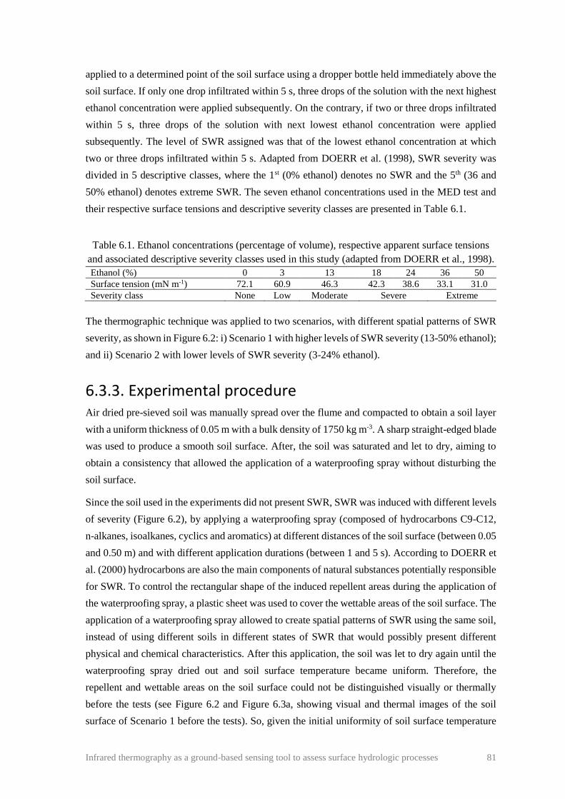
Infrared thermography as a ground-based sensing tool to assess surface hydrologic processes 81

applied to a determined point of the soil surface using a dropper bottle held immediately above the

soil surface. If only one drop infiltrated within 5 s, three drops of the solution with the next highest

ethanol concentration were applied subsequently. On the contrary, if two or three drops infiltrated

within 5 s, three drops of the solution with next lowest ethanol concentration were applied

subsequently. The level of SWR assigned was that of the lowest ethanol concentration at which

two or three drops infiltrated within 5 s. Adapted from DOERR et al. (1998), SWR severity was

divided in 5 descriptive classes, where the 1st (0% ethanol) denotes no SWR and the 5th (36 and

50% ethanol) denotes extreme SWR. The seven ethanol concentrations used in the MED test and

their respective surface tensions and descriptive severity classes are presented in Table 6.1.

Table 6.1. Ethanol concentrations (percentage of volume), respective apparent surface tensions

and associated descriptive severity classes used in this study (adapted from DOERR et al., 1998).

Ethanol (%) 0 3 13 18 24 36 50

Surface tension (mN m-1) 72.1 60.9 46.3 42.3 38.6 33.1 31.0

Severity class None Low Moderate Severe Extreme

The thermographic technique was applied to two scenarios, with different spatial patterns of SWR

severity, as shown in Figure 6.2: i) Scenario 1 with higher levels of SWR severity (13-50% ethanol);

and ii) Scenario 2 with lower levels of SWR severity (3-24% ethanol).

6.3.3. Experimental procedure Air dried pre-sieved soil was manually spread over the flume and compacted to obtain a soil layer

with a uniform thickness of 0.05 m with a bulk density of 1750 kg m-3. A sharp straight-edged blade

was used to produce a smooth soil surface. After, the soil was saturated and let to dry, aiming to

obtain a consistency that allowed the application of a waterproofing spray without disturbing the

soil surface.

Since the soil used in the experiments did not present SWR, SWR was induced with different levels

of severity (Figure 6.2), by applying a waterproofing spray (composed of hydrocarbons C9-C12,

n-alkanes, isoalkanes, cyclics and aromatics) at different distances of the soil surface (between 0.05

and 0.50 m) and with different application durations (between 1 and 5 s). According to DOERR et

al. (2000) hydrocarbons are also the main components of natural substances potentially responsible

for SWR. To control the rectangular shape of the induced repellent areas during the application of

the waterproofing spray, a plastic sheet was used to cover the wettable areas of the soil surface. The

application of a waterproofing spray allowed to create spatial patterns of SWR using the same soil,

instead of using different soils in different states of SWR that would possibly present different

physical and chemical characteristics. After this application, the soil was let to dry again until the

waterproofing spray dried out and soil surface temperature became uniform. Therefore, the

repellent and wettable areas on the soil surface could not be distinguished visually or thermally

before the tests (see Figure 6.2 and Figure 6.3a, showing visual and thermal images of the soil

surface of Scenario 1 before the tests). So, given the initial uniformity of soil surface temperature

82 Infrared thermography as a ground-based sensing tool to assess surface hydrologic processes

and of other characteristics (e.g. roughness, soil chemical characteristics, soil depth), the only

relevant characteristic that changes is the SWR induced on the soil surface.

Figure 6.2. SWR severity spatial patterns, in terms of percentage of ethanol, for the two tested

scenarios: a) Scenario 1; and b) Scenario 2. The photography of the soil surface of Scenario 1

after induced SWR (lower left corner) shows that repellent areas could not be visually

distinguished from wettable areas.

The proposed thermographic technique started by applying approximately 4.0 L of cold water, at a

temperature of 10-15 ºC (cooled in a refrigerator), over the soil surface. In previous studies of the

authors using infrared thermography to assess soil surface properties (DE LIMA and ABRANTES,

2014a; DE LIMA et al., 2014a, 2014b), hot water at a temperature of 80-85 ºC was used instead of

cold water. However, cold water was preferred in this study for its better performance and also its

easiness in future replication under field studies. The use of cold water in the field, will provide a

largest temperature contrast between soil and water, especially for dry and warm antecedent

weather conditions when SWR is expected to be most severe and, thus, to have greatest impact on

infiltration and runoff generation. The water was released manually by turning over the feeder box

located upslope of the flume (Figure 6.1). The feeder box was tipped in a quick and fast movement

in order to achieve a uniform discharge and a flow depth uniformity over the measuring area but,

at the same time, to induce minimum soil surface disturbances. The volume of water and consequent

applied discharge was adjusted to the conditions of the test (e.g. dimension of the measuring area,

slope, water temperature) and soil characteristics (e.g. permeability, roughness, macroporosity).

b) Scenario 2 a) Scenario 1

0.2 m 0.2 m

Scanned area

0% Ethanol

3% Ethanol

18% Ethanol

24% Ethanol

36% Ethanol

50% Ethanol

13% EthanolSlope

direction

0.2 m

Infrared thermography as a ground-based sensing tool to assess surface hydrologic processes 83

Thermal videos of the soil surface and water were recorded with the portable infrared video camera

throughout the tests. These videos were then analysed with the objective of identifying the repellent

and wettable areas. For each scenario, a thermogram (i.e. snapshot of the thermal video) was

selected and its temperatures were plotted against the corresponding SWR severity in terms of

percentage of ethanol classes. In order to map SWR severity spatial pattern with the thermographic

technique, the temperature of the thermograms was converted into percentage of ethanol classes

using a relation between the recorded temperatures and the actual SWR. Spatial patterns of

percentage of ethanol classes measured using the MED test and predicted on the basis of the

thermographic technique were then compared.

6.4. Results and discussion

Because the infrared camera converts the infrared radiation into temperature values based on the

materials emissivity coefficients, it should be noted that water and soil emissivity coefficients are

very similar in the operational spectral range of the present camera. Also, the proposed technique

does not aim to assess the exact actual temperatures of the soil surface and water but rather the

differences in temperature between repellent and wettable areas.

A chronological sequence of thermograms obtained for Scenario 1 (Figure 6.2a), from an instant

just before the cold water application to an instant after the passage of the water wave through the

scanned area is shown in Figure 6.3, illustrating how works the proposed technique. At the

beginning of the test (Figure 6.3a) soil surface temperature was almost uniform, with a mean value

of 26.3 ºC and a standard deviation of 0.4 ºC; therefore, it was not possible to distinguish between

wettable and repellent areas. As the water flowed down the flume over the soil surface (Figure

6.3b), it started to be repelled in the repellent areas (Figure 6.3c), starting to result in thermal

differences between warmer repellent areas and cooler wettable areas. After the passage of the

water wave through the measuring area (Figure 6.3d), repellent areas could be clearly distinguished

based on their lighter (reddish) colouration associated with higher temperatures (see colour scale

in Figure 6.3). Furthermore, stronger levels of SWR were associated with higher temperatures, as

illustrated in Figure 6.3 through the areas where SWR corresponded to the ethanol classes of 18

and 50%. After the water had exited from the soil flume (Figures 6.3e, 6.3f, 6.3g), thermal

differences between the wettable and repellent areas first increased for some instants. Then the

thermal differences again decreased when soil surface temperature became once more spatially

uniform as at the beginning of the test.

The imaging results were, in fact, driven by differences in soil water content, as observed in DE

LIMA et al. (2014b). Differences in soil water content were consequence of differences in SWR

severity. In wettable areas more cooled water flowed into the soil, therefore these areas presented

lower temperatures. Repellent areas presented higher temperatures, because less cooled water has

infiltrated in these places.

84 Infrared thermography as a ground-based sensing tool to assess surface hydrologic processes

Figure 6.3. Chronological sequence of thermograms obtained during the application of the

thermographic technique in Scenario 1: a) Instant just before the water application (0 s) where

repellent areas cannot be identified; b) During the passage of the cold water wave (0.5 s); and c)

d) e) f) and g) After the passage of the water wave through the scanned area (1.0, 1.5, 2.0, 2.5 and

3.0 s).

The thermograms of the two tested scenarios after the passage of the water wave through the

scanned area (i.e. 3 s after the water application) are shown in Figure 6.4. This specific instant was

chosen because it revealed the strongest thermal differences between the wettable and repellent

areas and, thus, allowed evaluating the best possible performance of the proposed technique. Both

thermograms allowed to distinguish repellent areas from wettable areas. Areas with higher SWR

severity were more clearly perceptible than areas with lower SWR severity, as was evident from a

comparison of the two thermograms with the scenarios’ respective spatial SWR patterns (see

Figure 6.2). Areas with severe and extreme SWR, which were more frequent in Scenario 1 than in

Scenario 2, revealed the highest recorded temperatures. In contrast, some of the areas with low

SWR in Scenario 2, especially those located on the 2nd and 6th rows, could not be distinguished in

terms of soil surface temperature from wettable areas. Likewise, in DE LIMA et al. (2014b), while

higher surface soil permeability differences were clearly perceptible, smaller differences were not

so easily detected.

a)

e)

b) c) d)

f) g)

0 s

2.0 s

0.5 s 1.0 s 1.5 s

2.5 s 3.0 s

25.8 ºC 13.0 ºC 14.1 ºC 14.6 ºC

15.1 ºC

20.4 ºC

18.9 ºC

15.6 ºC

21.8 ºC

19.3 ºC

15.8 ºC

22.2 ºC

17.2 ºC

26.4 ºC

26.3 ºC

14.4 ºC

13.6 ºC

14.8 ºC

13.9 ºC

18.3 ºC

15.9 ºC0.2 m

0.2 m

0.2 m

0.2 m

0.2 m

0.2 m

0.2 m

30 ºC20 ºC10 ºC

0% Ethanol

18% Ethanol

50% Ethanol

Surface flow

direction

26.7 ºC

25.9 ºC

14.6 ºC

12.8 ºC

15.0 ºC

15.5 ºC

15.6 ºC

18.4 ºC

16.2 ºC

19.6 ºC

16.6 ºC

20.5 ºC

16.9 ºC

20.9 ºC

Infrared thermography as a ground-based sensing tool to assess surface hydrologic processes 85

Figure 6.4. Thermograms of the soil surface of 3 s after the water application for the two tested

scenarios: a) Scenario 1; and b) Scenario 2. Notice that the colour scale is different from the one

in Figure 6.3.

The thermograms revealed some deformations of the rectangular areas where SWR was induced,

suggesting a leaching of SWR from these areas in the downslope direction. These deformations

could be artefacts of the present technique but, at the same time, could also reflect heat diffusion,

or transport of repellent soil particles by the water wave, as observed in DE LIMA and ABRANTES

(2014a) and in DE LIMA et al. (2014b). The thermograms also revealed a tendency to record higher

temperatures in the right side of the measuring area, which was attributed to a slightly lower flow

depth in this region during the passage of the cold water through the measuring area.

Figure 6.5 presents the frequency distribution of the temperature, in classes of 5 ºC, and their

median values, plotted against the seven percentage of ethanol classes. In the case of both scenarios,

the median temperatures increased monotonically with increasing ethanol class and, thus, level of

SWR. Furthermore, the median temperature for each ethanol class differed little between the two

scenarios, attesting to the reproducibility of results between different experiments. Worth

mentioning in this respect is that small variations in both soil surface temperature and the

temperature of the applied water are difficult to avoid, and, in this particular case, could help explain

the differences in the temperature distributions between the two scenarios, most noticeably at the

ethanol class of 24%.

a) Scenario 1 b) Scenario 2

0.2 m 0.2 m

25 ºC20 ºC15 ºC

Surface flow

direction

86 Infrared thermography as a ground-based sensing tool to assess surface hydrologic processes

Figure 6.5. Temperature frequency distributions (classes of 5 ºC), and median temperatures

plotted against the corresponding percentage of ethanol classes.

Figure 6.6 illustrates the two empirical functions for converting the temperatures extracted from

the thermograms into percentage of ethanol classes. Both functions were derived from the

information shown in Figure 6.5, assuming that the median temperatures varied linearly between

two consecutive percentage of ethanol classes and that the midpoints of the linear variations defined

the boundaries of the functions for each class. The lower and upper boundaries, respectively of the

lower and higher percentage of ethanol classes, corresponded to the minimum and maximum

recorded temperatures.

Applying in turn these functions to the thermograms allowed mapping the spatial patterns of SWR

for both scenarios, as shown in Figure 6.7. A single empirical function covering the conditions of

the two scenarios would be more valuable. However, the two scenarios did not presented the same

levels of SWR (Scenario 1 presented SWR levels from 3 to 24% of ethanol and Scenario 2 presented

SWR levels from 13 to 50% of Ethanol). Therefore, if such single empirical function was applied

levels of SWR that only exist in Scenario 1 will also appear in Scenario 2 and vice versa.

Figure 6.8 compares the percentage of ethanol as measured using the MED test with those predicted

on the basis of the thermograms and derived empirical functions. This is done for some longitudinal

and transversal cross sections of the scanned area. The thermography based predictions were more

reliable in the cases of none and medium to extreme SWR, even though medium to severe ethanol

classes were often overestimated. This overestimating effect was observed in previous studies of

the authors (DE LIMA and ABRANTES, 2014a; DE LIMA et al., 2014b). In the case of low SWR

its presence was not always correctly predicted.

0 25 50 0 25 50 0 25 50 0 25 50 0 25 50 0 25 50 0 25 50

15

16

17

18

19

20

21

22

23

24

25

0 3 13 18 24 36 50

Ethanol (%)

Tem

per

atu

re(º

C)

Frequency distribuition (%)

Medium

SWR

No

SWRSevere SWR Extreme SWR

Low

SWR

Temperature frequency distribuition

Scenario 2

Scenario 1

Median temperature

Scenario 2

Scenario 1

Infrared thermography as a ground-based sensing tool to assess surface hydrologic processes 87

Figure 6.6. Empirical functions (filled areas) used to convert temperature data into percentage of

ethanol classes: a) Scenario 1; and b) Scenario 2.

Figure 6.7. SWR spatial distribution, in terms of percentage of ethanol, obtained with the

thermographic technique: a) Scenario 1; and b) Scenario 2. See corresponding thermograms in

Figure 6.4.

Ethanol (%)

Tem

per

atu

re(º

C)

1516171819202122232425

0 13 18 24 36 50

Scenario 1a)

Low

SWR

No

SWR

Medium

SWR

Severe

SWR

1516171819202122232425

0 3 13 18 24

b) Scenario 2T

emp

era

ture

(ºC

)

Medium

SWR

No

SWR

Severe

SWR

Extreme

SWR

Empirical function

Scenario 2

Scenario 1

Median temperature

Scenario 2

Scenario 1

b) Scenario 2 a) Scenario 1

0.2 m 0.2 m

24% Ethanol

36% Ethanol

50% Ethanol

Surface flow

direction

0% Ethanol 18% Ethanol

13% Ethanol

3% Ethanol

88 Infrared thermography as a ground-based sensing tool to assess surface hydrologic processes

Figure 6.8. Comparison of SWR, in terms of percentage of ethanol, predicted on the basis of

thermography and measured using the MED test, along longitudinal and transversal cross sections

shown in the upper right corner of the plots (see SWR spatial distribution obtained with

thermography and measured with the MED test in Figures 6.2 and 6.7).

6.5. Conclusions

In the present small-scale exploratory laboratory study, a technique based on infrared thermography

was tested for assessing water repellency at the soil surface (SWR) and mapping its spatial

variability. The technique proved to be of easy and fast application and, in overall terms, successful

in distinguishing areas that were water repellent from areas that were wettable as well as in

distinguishing between areas with different levels of SWR, in particular, between areas with

extreme as opposed to low to medium SWR.

The proposed technique, however, also presented some drawbacks: i) It performed poorly in

identifying areas with low SWR; ii) It may require measurements of SWR as a basis for accurate

0

10

20

30

40

50

0 0.1 0.2 0.3 0.4 0.5 0.6 0.7 0.8

0

10

20

30

40

50

0 0.1 0.2 0.3 0.4 0.5 0.6

0

10

20

30

40

50

0 0.1 0.2 0.3 0.4 0.5 0.6 0.7 0.8

c) Scenario 1

0

10

20

30

40

50

0 0.1 0.2 0.3 0.4 0.5 0.6

0

10

20

30

40

50

0 0.1 0.2 0.3 0.4 0.5 0.6

a) Scenario 1E

than

ol

(%)

b) Scenario 1

d) Scenario 2

Eth

an

ol

(%)

f) Scenario 2e) Scenario 2

Eth

an

ol

(%)

Distance (m) Distance (m)

0

10

20

30

40

50

0 0.1 0.2 0.3 0.4 0.5 0.6

MED testThermography

– Scenario 1

Thermography

– Scenario 2

Infrared thermography as a ground-based sensing tool to assess surface hydrologic processes 89

predictions, as the underlying equation may depend strongly on local soil conditions as well as

experimental aspects (e.g. temperature of the applied water); iii) It may interfere with the spatial

SWR patterns themselves, by leaching, and, as such, is not necessarily a non-destructive technique;

and iv) It may also affect the soil surface characteristics, especially in easily erodible soils.

Overall, the proposed technique apparently has high potential to contribute to a better understanding

of the hydrological impacts of different spatial patterns of SWR due to its capacity to monitor in

real time the dynamics of these impacts (e.g. establish critical thresholds when SWR is diminished,

i.e. to look into when SWR areas turn from runoff sources to runoff sinks).

Results of this exploratory study suggest that is worthwhile to explore this technique in the field.

Only extensive field work can, in fact, reveal the suitability of the technique in real conditions.

Further work is therefore suggested for a more robust assessment of the applicability of the

proposed technique, under field conditions with the presence of natural SWR. Future testing should

analyse the impacts of applying different amounts of water and in different regimes, and evaluate

the technique at different spatial scales and for different spatial patterns of SWR as well as different

soil surface conditions in terms of, e.g. random roughness and cover of stones and mulch, which is

beyond the scope of the presented analysis. Also, future tests should include SWR measurements

with other techniques, such as the WDPT test, and measurements of soil water content to study its

relation with the SWR.

“Each soil has had its own history. Like a river, a mountain, a forest, or any natural thing, its

present condition is due to the influences of many things and events of the past.”

- Charles Kellogg

Infrared thermography as a ground-based sensing tool to assess surface hydrologic processes 93

7. FIELD ASSESSMENT OF SOIL WATER REPELLENCY USING INFRARED THERMOGRAPHY5

7.1. Abstract

This study aimed to evaluate the applicability of an infrared thermography technique relying on

cooling the soil surface with cold water for assessing soil water repellency (SWR) severity under

field conditions. This study is a follow-up of earlier exploratory small-scale laboratory tests, where

SWR spatial variability was mapped and repellent areas could be clearly detected on the thermal

imaging due to their higher temperatures, thus distinguishing them from the remaining wettable

areas.

Field tests were carried out, where both natural and artificial SWR were mapped through thermal

imaging, using a portable infrared video camera. Cold water was used to create a temperature

gradient on the soil surface in order to assess SWR. Naturally repellent soils were found in a pine

and eucalyptus forest and artificial SWR was induced with a waterproofing spray. The molarity of

an ethanol droplet (MED) test was used to measure both natural and artificial SWR severity.

The technique was, in overall terms, successful in mapping SWR spatial variability, distinguishing

repellent from wettable areas as well as distinguishing different levels of SWR severity. Only

extensive testing can, ultimately, validate the technique and reveal its suitability in different field

conditions (e.g. surface roughness, surface cover, spatial scale).

Keywords Soil water repellency; Infrared thermography; Field tests

7.2. Introduction

Soil water repellency (SWR) is recognized as a key hydrological and geomorphological process

since the earlier part of the 20th century. However, first observations of this phenomenon were

reported in the later part of the 18th century (DEBANO, 2000a, DOERR et al., 2000). SWR is a

major concern to hydrogeologists and land managers since it can alter infiltration and solute

5 ABRANTES, J.R.C.B., DE LIMA, J.L.M.P., PRATS, S.A. and KEIZER, J.J. (2016). Field assessment of

soil water repellency using infrared thermography. Forum Geographic, 15(2), 12-18.

DOI:10.5775/fg.2016.019.s.

94 Infrared thermography as a ground-based sensing tool to assess surface hydrologic processes

transport into the soil, enhancing surface runoff and associated erosion and affecting seed

germination and plant growth, triggering land degradation processes (KEIZER et al., 2005b;

LEIGHTON-BOYCE et al., 2007; RITSEMA and DEKKER, 1994; SHAKESBY et al., 1993).

SWR is originated by the coating of soil particles with hydrophobic organic substances usually

released by plants or decomposing plant material (DEKKER and RITSEMA, 1994; KEIZER et al.,

2005c). Repellent soils have been found in fire affected forest lands (BADÍA-VILLAS et al., 2014;

KEIZER et al., 2008; MATAIX-SOLERA and DOERR, 2004), but also in pine and eucalypt forest

lands not affected by fires and in agricultural lands with high soil organic matter content (DOERR

et al., 2000, KEIZER et al., 2007, SANTOS et al., 2013).

One of the most commonly used technique to measure SWR is the Molarity of an Ethanol Droplet

(MED) test (LETEY, 1969), which measures the surface tension between an ethanol solution and

the soil surface to indirectly determine how strongly the water is repelled. It provides quantitative

data, but the subsequent classification or characterization of these data varies with the objective of

the investigator and perception of what constitutes low or high SWR severity. The MED test is a

practical and quick test and has therefore been widely applied in especially intensive field

monitoring studies (KEIZER et al., 2005c; 2007, 2008; MALVAR et al., 2016; SANTOS et al.,

2013). Other techniques used to measure SWR include measurement of the time taken by a water

drop to completely penetrate into the soil, measurement of the water-soil contact angle,

measurement of ethanol and water ethanol sorptivity, measurement of the water entry pressure head

of a soil and the sessile drop method (DEKKER et al., 2009; KING, 1981). However, these

techniques only provide punctual data that must be grouped or scaled to bring out spatial coherence,

in order to properly map spatial variations of SWR at field and landscape scales.

Infrared thermography based methods have been used as high resolution imaging tools in hydrology

(BONAR and PETRE, 2015; MEJÍAS et al., 2012; SCHUETZ et al., 2012) and physical geography

(DEHVARI and HECK, 2007; POHL and VAN GENDEREN, 1998; RICCHETTI, 2001), in

particular those using portable hand-held infrared cameras have been increasing due to recent

reductions in their prices and substantial enhancements of their portability and spatial resolution.

In recent studies, infrared thermographic techniques were used by the authors to assess different

soil surface hydrological processes in laboratory and field conditions (ABRANTES and DE LIMA,

2014; ABRANTES et al., 2017; DE LIMA and ABRANTES, 2014a, 2014b; DE LIMA et al.,

2014a, 2014b, 2014c, 2015a, 2015b).

This study aimed to evaluate the applicability of a field infrared thermography technique relying

on cooling the soil surface with cold water for assessing small-scale SWR severity under field

conditions. This study is a follow-up of exploratory small-scale laboratory tests presented in

ABRANTES et al. (2017) where SWR spatial variability was mapped and repellent areas could be

clearly detected on the thermal imaging due to their different coloration associated with higher

temperatures, thus distinguishing them from the remaining wettable areas.

Infrared thermography as a ground-based sensing tool to assess surface hydrologic processes 95

7.3. Study area and soil surface repellency

The field tests presented in this study (Figure 7.1) were conducted in a Pine (P. pinaster) and

Eucalyptus (E. globulus) forest site located in Pinhal de Marrocos, Coimbra, Portugal, in the

surroundings of the Department of Civil Engineering of the Faculty of Sciences and Technology of

the University of Coimbra. The soils in this site were loamy sand soils with a surface slope between

15-20%. Soil surface was dry at the beginning of the tests.

Figure 7.1. Photographs of: a) study area with observation of the increasing layer of litter and,

consequently, increasing SWR; b) and c) scenarios 5 and 6, respectively, with representation of

the boundary between the wettable and the induced repellent areas (photographs taken

immediately after application of the waterproofing spray); and d) location of the places where the

MED test was used to measure the SWR in the scanned area, after removal of the litter layer.

The thermographic technique was tested in 6 areas of the study site, each with approximately

0.65 × 0.85 m2. The areas presented different characteristics (Figure 7.1a), such as areas with bare

soil surface in open patches of the tree canopy (i.e. wettable soil surface) and areas with soil surface

covered with a thick litter layer of pine and eucalyptus residues (i.e. repellent soil surface). Some

wettable areas of the soil surface were also induced with artificial repellency by applying a

waterproofing spray. This allowed to test the technique in different soil surface repellent conditions,

ranging from wettable to extremely repellent: scenario 1 with wettable soil surface; scenario 2 with

low SWR; scenario 3 with moderate SWR; scenario 4 with severe SWR; scenario 5 with half of the

96 Infrared thermography as a ground-based sensing tool to assess surface hydrologic processes

area artificially induced with extreme repellency (Figure 7.1b); and scenario 6 with circular areas

artificially induced with extreme repellency (Figure 7.1c).

SWR severity was determined at the soil surface after removal of the litter layer, using the MED

test (following proceeding used in ABRANTES et al., 2017). SWR severity was divided in 5

repellency intensity classes, according to the ethanol concentration, as follows (adapted from

DOERR et al., 1998): class 0, wettable (0%); class 1, low repellency (1, 3 and 5%); class 2,

moderate repellency (8.5 and 13%); class 3, severe repellency (18 and 24%) and class 4, extreme

repellency (36, 50% and more). In each scenario, SWR measurements were conducted randomly

at the soil surface on 16 points in a regular pattern, as shown in Figure 7.1d.

7.4. Infrared thermographic technique

A schematic representation of the experimental setup used in this study is presented in Figure 7.2.

The proposed thermographic technique tested previously in laboratory (ABRANTES et al., 2017),

started by applying approximately 4.0 L of cold water, at a temperature of 6.3 ± 0.5 ºC (cooled in

a refrigerator), over the soil surface. The water was released manually by turning over a feeder box

located upslope of the scanned area (Figure 7.2). The feeder box was tipped in a quick and fast

movement in order to achieve a uniform discharge and a flow depth uniformity over the scanned

area but, at the same time, to induce minimum soil surface disturbances.

Figure 7.2. Scheme of the setup used in the field tests (not at scale).

Thermal videos of the soil surface and water were recorded with an Optris PI-160 portable infrared

video camera (Optris GmbH, Germany) with an optical resolution of 160 × 120 pixels. The camera

was attached to a support structure with the focal direction perpendicular to the soil surface, at a

distance of 2.15 m (Figure 7.2).

These videos were then analysed with the objective of distinguish repellent from wettable areas as

well as identify different levels of SWR. For each scenario, two thermograms (i.e. snapshot of the

thermal video) were selected and its temperatures were analysed: one corresponding to an instant

Infrared thermography as a ground-based sensing tool to assess surface hydrologic processes 97

just before the cold water application; and other corresponding to an instant just after the passage

of the cold water wave through the scanned area, approximately 5 s after the cold water application.

This specific instant was chosen because, in general, it revealed the strongest thermal differences

between wettable and repellent areas and, thus, allowed evaluating the best possible performance

of the proposed technique.

7.5. Results and discussion

Thermograms of the six scenarios studied in the field experimental tests, using the proposed

infrared thermography technique, are presented in Figure 7.3. Each thermogram comprises a total

of 19200 pixels (i.e. temperature data points), each one with a size of 28.8 mm2.

At the beginning of the tests, soil surface temperature was not exactly the same in all scenarios.

Average soil surface temperature of scenarios with previous presence of a litter layer of forest

residues (removed at the beginning of the tests and before thermal images were captured) was lower

than bare soil scenarios (average values of 22.2 and 24.0 ºC, respectively). Before the application

of the thermographic technique (i.e. application of the cold water on the soil surface), the extremely

repellent area induced with waterproofing spray could not be distinguished from the wettable area

in scenario 5 (Figure 7.3e left). However, circular extremely repellent areas, induced with

waterproofing spray, in scenario 6 showed slightly lower temperatures than the remaining wettable

area. Even so, these thermal differences were not significant and, by themselves, were not sufficient

to identify the extremely repellent areas.

As the cold water flowed down the scanned areas, it started to be repelled in the repellent areas.

Therefore, after the passage of the water wave through the scanned areas, scenarios with stronger

levels of SWR presented higher average temperatures (cold water was repelled), as opposed to

scenarios with no (wettable soil) and lower levels of SWR, where more cold water infiltrated into

the soil, thereby cooling it. Extremely repellent areas induced with waterproofing spray in scenarios

5 and 6 (Figures 7.3e and 7.3f) could be clearly distinguished from the wettable area, based on their

lighter colouration associated with higher temperatures (also observed in ABRANTES et al., 2017).

Imaging results were driven by soil water content as a result of infiltration differences (also

observed in DE LIMA et al., 2014b). As stated before, in wettable areas more cooled water flowed

into the soil, therefore these areas presented lower temperatures. Repellent areas presented higher

temperatures, because less cooled water has infiltrated in these places since it was repelled.

Therefore, these imaging results are a clear indicator of the drainage pattern of each studied

scenario, especially Figures 7.3c and 7.3d.

98 Infrared thermography as a ground-based sensing tool to assess surface hydrologic processes

Figure 7.3. Unprocessed soil surface thermograms of the six scenarios studied in the field tests,

before (ti = 0 s) and after (tf = 5 s) the application of the thermographic technique (i.e. application

of the cold water on the soil surface): a) scenario 1 with wettable soil surface; b) scenario 2 with

low SWR; c) scenario 3 with moderate SWR; d) scenario 4 with severe SWR; e) scenario 5 with

half of the area artificially induced with extreme repellency; and f) scenario 6 with circular areas

artificially induced with extreme repellency.

Since the application of the thermographic technique only lasted 5 s (i.e. time taken from the

application of the cold water to its passage through the scanned area), temperature exchange

between the soil surface (and/or water flowing at the soil surface) and the atmosphere was

considered negligible.

Infrared thermography as a ground-based sensing tool to assess surface hydrologic processes 99

The thermogram of scenario 6 presented some deformations of the circular areas, where extreme

SWR was induced, suggesting leaching of SWR from these areas in the downslope direction (also

observed in ABRANTES et al., 2017). These deformations could result/reflect the transport of

repellent soil particles by the water wave and/or heat diffusion, as observed in DE LIMA and

ABRANTES (2014a) and DE LIMA et al. (2014b).

As stated before, soil surface temperature at the beginning of the tests (i.e. prior to cold water

application) was not exactly the same in all scenarios; therefore, the temperature in the thermograms

was corrected by subtracting the temperature of the thermograms before the cold water application

(Ti at ti = 0 s) to the temperature of the thermograms after the cold water application (Tf at tf = 5 s),

as schematized in Figure 7.4 for scenario 1. Since the temperature of the cold water applied to the

soil surface was approximately equal in all tested scenarios (6.3 ± 0.5 ºC) a correction of this

temperature was not done. However, a similar correction should be considered if the temperature

of the applied water would not equal.

Figure 7.4. Scheme of the procedure used in the temperature correction of the soil surface

thermograms, for scenario 1.

The correction procedure resulted in the final thermograms is shown in Figure 7.5, for all tested

scenarios. With this correction, temperature of all thermograms can be compared without

interference of the initial temperature of the soil surface. This is relevant because average soil

surface temperature of scenarios with previous presence of a litter layer of forest residues was lower

than bare soil scenarios.

As shown in Figure 7.5, scenarios with stronger levels of SWR presented a corrected temperature

(i.e. temperature difference) closer to 0 ºC, since its final temperature was more similar to the initial

temperature, due to lower cold water infiltration. By contrast, scenarios with no and lower levels

of SWR presented average lower corrected temperatures, due to higher infiltration of cold water

into the soil. This is shown in the graph of the Figure 7.5g which presents the average corrected

temperatures, extracted from the processed thermograms, and plotted against the 5 SWR severity

classes measured with the MED test.

100 Infrared thermography as a ground-based sensing tool to assess surface hydrologic processes

Figure 7.5. a), b), c), d), e) and f) Thermograms of the soil surface after the correction procedure,

for all tested scenarios; and g) Average and standard deviation (19200 data points) of the

corrected temperatures plotted against the 5 SWR severity classes measured with the MED test

(class 0 – wettable, class 1 - low SWR, class 2 - moderate SWR, class 3 - severe SWR and class 4

- extreme SWR).

Figure 7.6 shows corrected temperatures extracted from the thermograms, for some cross sections

of the scanned area, for all tested scenarios. The longitudinal (Figure 7.6a) as well as transversal

(Figure 7.6b) cross sections revealed that average corrected temperatures contrasted markedly

between scenarios 1, 2 and 3-4. However, almost no difference was observed between the average

corrected temperature of scenarios 3 and 4. For the induced extreme SWR scenarios (scenario 5 in

Figure 6c and scenario 6 in Figure 7.6d) a clear distinction existed between the corrected

temperature in the repellent and wettable areas.

Infrared thermography as a ground-based sensing tool to assess surface hydrologic processes 101

Figure 7.6. Soil surface corrected temperature (data points and average lines), for some cross

sections of the scanned area (shown in the right side of the plots): a) Longitudinal cross sections

for scenarios 1, 2, 3 and 4 (160 data points); b) Transversal cross sections for scenarios 1, 2, 3 and

4 (120 data points); c) Cross section for scenario 5 (90 data points); and d) Cross section for

scenario 6 (60 points).

7.6. Conclusion

In the present field study, a technique based on infrared thermography was tested for assessing

water repellency at the soil surface (SWR). The technique proved to be an easy and fast way for

gathering a high resolution SWR map in small scale field plots, allowing thermograms with 19200

data points versus the 16 MED measurements. The technique was, in general, successful in

distinguishing areas that were water repellent from areas that were wettable as well as in

distinguishing between areas with different levels of SWR. Overall, the proposed technique

102 Infrared thermography as a ground-based sensing tool to assess surface hydrologic processes

apparently has high potential to contribute to a better understanding of the hydrological impacts of

SWR, by also revealing the drainage pattern of the field plots.

However, the proposed technique presented some drawbacks: i) It may require measurements of

SWR as a basis for accurate predictions; ii) It can only be applied to relatively flat sloping soil

surfaces and its results may depend strongly on experimental aspects (e.g. temperature of applied

water), as well as on local soil conditions, such as roughness, temperature, moisture and

macroporosity, which could create preferential infiltration patterns even in highly repellent areas;

and iii) It may affect the soil surface characteristics, especially in easily erodible soils and it may

alter SWR levels and, especially through leaching, SWR spatial patterns.

Results of this study suggest that is worthwhile to explore this technique. Only extensive testing

can, in fact, validate the technique and reveal its suitability under different field conditions

(e.g. surface roughness, surface cover, spatial scale).

“The movement of heavenly bodies despite their distance from earth have presented fewer

difficulties to me than the movement of water which is within my reach.”

- Galileo

Infrared thermography as a ground-based sensing tool to assess surface hydrologic processes 105

8. USING A THERMAL TRACER TO ESTIMATE OVERLAND AND RILL FLOW VELOCITIES6

8.1. Abstract

Flow velocity is a basic hydraulic property of surface flows and its precise calculation is necessary

for process based hydrological models, such as soil erosion and rill development models, as well

as for modelling sediment and solute transport by runoff. This study presents a technique based on

infrared thermography to visualize very shallow flows and allow a quantitative measurement of

overland flow and rill flow velocities. Laboratory experiments were conducted to compare the

traditional dye tracer technique with this new thermal tracer technique by injecting a combined

tracer (heated dye) into shallow flowing surface water.

The leading edge tracer velocities estimated by means of infrared video and by the usual real

imaging video were compared. The results show that thermal tracers can be used to estimate both

overland and rill flow velocities, since measurements are similar to those resulting from using dye

tracers. The main advantage of using thermography was the higher visibility of the leading edge of

the injected tracer compared with the real image videos.

Keywords Shallow flow velocity; Thermal tracer; Infrared thermography

8.2 Introduction

Shallow flows (e.g. overland flow, rill flow) often occur in natural and urbanized drainage basins

and have important implications (e.g. water erosion, water quality). The understanding and

modelling of these flows are necessary in surface hydrology and soil and water conservation

studies. Flow velocity is a basic hydraulic property of overland flow and its precise calculation is a

necessary component of all process based hydrological models such as soil erosion and rill

development models (e.g. GOVERS, 1992; GIMÉNEZ et al., 2004; WIRTZ et al., 2012), as well

as in modelling sediment and solute transport by runoff (e.g. LEI et al., 2010; MÜGLER et al.,

2011).

6 DE LIMA, J.L.M.P. and ABRANTES, J.R.C.B. (2014). Using a thermal tracer to estimate overland and rill

flow velocities. Earth Surface Processes and Landforms, 3(10), 1293-1300. DOI:10.1002/esp.3523.

106 Infrared thermography as a ground-based sensing tool to assess surface hydrologic processes

For a long time, common techniques used in shallow flow velocity measurements for soil erosion

studies were based on the determination of the travel time of a tracer across a defined section, in

both laboratory (e.g. ABRAHAMS and ATKINSON, 1993; GIMÉNEZ and GOVERS, 2002) and

field conditions (e.g. HORTON et al., 1934; WIRTZ et al., 2012). More recently, a tracer technique

that combined high speed digital cameras and laser scanners, and called Large Scale Particle Image

Velocimetry (LSPIV), was used to estimate the temporal and spatial variability of shallow flow

velocities and flow depths (e.g. JODEAU et al., 2008; KIM et al., 2008; LEGOUT et al., 2012).

According to FLURY and WAI (2003) an ideal water tracer has the following characteristics:

i) Movement similar to water, without sorption to soils, sediments or rocks and without degradation

during the measurement time; ii) Low background concentration, i.e. clearly discernible from the

background of the system; iii) Behaviour unaffected by changes in the water chemistry (e.g. pH);

iv) Detectable either by chemical analysis or by visualization; and v) Low toxicological impact on

the study environment. Different materials have been tested as water tracers in flow velocity

experiments (e.g. chemicals, gases, natural and radioactive isotopes, magnetized materials,

fluorescent particles, floating objects, dyes, electrolytes). Dyes of different colours, fluorescent

dyes, fluorescent particles and electrolytes are the tracer materials most often used to measure flow

velocity in soil erosion studies (e.g. ABRAHAMS et al., 1986; LEI et al., 2005, 2010; SHI et al.,

2012; TATARD et al., 2008; TAURO et al., 2012a, 2012b). The usual procedure to estimate the

mean flow velocity with dye and electrolyte tracers is to measure the time from the injection of the

tracer to the arrival of the leading edge of the tracer concentration at a sampling point and then

divide this figure by the travel distance to give the leading edge velocity. The travel time of the

leading edge of the tracer concentration is usually observed visually in the case of dye tracers and

is measured using an electric conductivity sensor in the case of salt tracers. The leading edge

velocity is then multiplied by a correction factor to obtain the mean flow velocity

(e.g. DUNKERLEY, 2001; LI et al., 1996; ZHANG et al., 2010).

Infrared thermography has been successfully employed in hydrological studies as a high spatial and

temporal resolution non-intrusive imaging tool to measure water surface temperatures and detect

thermal sources: e.g. infrared thermography techniques were used to detect and quantify discharges

of groundwater and freshwater into nutrient-sensitive estuaries and coastal bays

(e.g. DANIELESCU et al., 2009; MEJÍAS et al., 2012). In particular, more field studies with

portable hand-held infrared thermography systems have been carried out recently because the

equipment is easy to handle and the measurement distance and scale are easy to adjust (e.g.

CARDENAS et al., 2008; PFISTER et al., 2010; SCHUETZ et al., 2012).

Some authors have studied the use of infrared thermography and thermal tracers to measure shallow

flow velocities. SCHUETZ et al. (2012) used infrared thermal imaging combined with the injection

of heated water as an artificial tracer technique to characterize the spatial distribution of flow paths

and to assess transport properties in a 65 m2 experimentally constructed wetland with water depths

between 0.1-0.2 m. For the studied conditions the authors observed that heated water can be used

Infrared thermography as a ground-based sensing tool to assess surface hydrologic processes 107

as a conservative artificial tracer for plot scale experiments. LIANG et al. (2012) studied the

feasibility of using thermal imaging to investigate the scalar transport process in shallow jet and

wake flows with waters depths of 35 mm and 45 mm by adding warm water to the water flow. The

authors found that the thermal imaging technique has great potential as a quantitative flow

visualisation technique for studying shallow turbulent dispersion characteristics.

The purpose of this study is to describe a technique based on infrared thermography to visualize

very shallow flows and enable a quantitative measurement of overland flow and rill flow velocities.

Laboratory experiments were conducted to compare the traditional dye tracer technique with this

new thermal tracer technique by injecting a combined tracer (heated dye) into these shallow flowing

surface waters. In fact, for these deeper flows, dye tracing is considered by many a crude method

that yields a maximum flow speed that has to be scaled to yield mean speed. However, in these

muddy flows, with depths of a few millimetres, it is not possible to use far more sophisticated

methods of measuring true mean flow speed that are reported in the literature for surface flows,

namely river flows. In this study the leading edge tracer velocities estimated by means of infrared

video and by a regular real imaging video were compared. The novelty of the proposed technique

for computing mean velocity of overland flow and rill flow lies in the tracer characteristics. A

thermal tracer is used instead of a dye tracer. The scientific question that arises from this paper is:

Can a thermal tracer be used to estimate very shallow flow velocities?

8.3. Materials and methods

8.3.1. Laboratory set-ups Two slightly different laboratory set-ups were used for the qualitative and quantitative comparison

of the thermal tracer technique and dye tracer technique, one for the estimation of overland flow

velocity (Figure 8.1a) and the other for rill flow velocity estimation (Figure 8.1b). Both experiments

were carried out in a 3.0 m long and 0.3 m wide soil flume, adjusted to a 10% slope, with a water

supply system installed upstream of the flume. The water supply system comprised a constant head

tank and a feeder tank and allowed the application of a known constant flow of water to the flume

soil surface.

8.3.2. Soil The soil was a sandy loam collected from the banks of River Mondego (Coimbra, Portugal),

exhibiting clear signs of water erosion (e.g. DE LIMA et al., 2003). The soil consisted of 7% clay,

9% silt and 84% sand and was mainly composed of quartz, feldspars, quartzite, muscovite and clay

minerals. Standard laboratory permeability tests estimated saturated hydraulic conductivity of

around 5.7 × 10-5 m s-1. The sieved soil was uniformly spread in the flume, positioned horizontally,

and a sharp straight-edged blade was used to remove excess soil to obtain a flat plane surface. The

108 Infrared thermography as a ground-based sensing tool to assess surface hydrologic processes

soil in the flume was gently tapped with a wooden block to compact it and to reproduce a uniform

bulk density of approximately 1700 kg m-3. The soil was then saturated and left to dry until it gained

a consistency that allowed the eroding effect of the water flux to be minimized and so preserve the

soil surface characteristics throughout the experiments.

Figure 8.1. Schematic representation of the laboratory set-up (not to scale) for: a) Overland flow

tests; and b) Rill flow tests.

The first series of experiments to measure overland flow velocity were performed on the uniformly

smooth plane surface, without any rough protuberances or other microtopographic elements. For

the second set of experiments an artificial rill was created along the length of the flume by

compressing a malleable plastic form against the soil surface. The rill had an average depth of

Infrared thermography as a ground-based sensing tool to assess surface hydrologic processes 109

8.9 ± 0.3 mm and width of 16.4 ± 2.3 mm and was fixed by spreading sieved white cement powder

over the entire rill.

8.3.3. Tracers To be able to compare the flow velocities measured with the thermal tracer and the dye tracer, the

two techniques were tested simultaneously in a combined tracer comprising both dye and thermal

characteristics. This was accomplished by heating the dye tracer solution, well above the average

surface flow water temperature which varied from 18 ºC to 20 ºC.

In the first set of experiments (overland flow tests), non-fat milk heated to a temperature of

approximately 80 ºC was used as a combined tracer. Non-fat milk was used because it can be heated

to high temperatures and it is visible when injected into the water flow due to the dark brownish

colour of the wetted soil surface. Also, it presents a similar density to other tracer solutions. In the

rill flow tests, heated blue litmus tracer at a temperature of approximately 80 ºC was used as a

combined tracer, due to the contrast with the whitish colour of the surface. The temperature of 80 ºC

was used for convenience: after heating the water in an electric kettle, it was transferred to the cups

for application on the flow.

Differences in water density and viscosity, which change slightly with temperature, do not seem to

have a visible influence on the dispersion of the dye tracer in these experiments, due to: i) Small

injected tracer volume (< 22 ml for overland flow and < 5 ml for rill flow); ii) Short sampling time

(< 4 s for overland flow and < 2 s for rill flow); and iii) Short sampling length (0.5 m). Relative

differences between tracer leading edge velocities measured with the same dye tracer at 15 ºC and

85 ºC were always less than 8%, under the tested experimental conditions, which is similar to the

relative errors for the same temperature. This is explained by the variability induced by the manual

implementation of this technique.

8.3.4. Video recording systems Thermal videos and imaging of the soil surface and water were recorded with an Optris PI 160

portable infrared video camera (Optris GmbH, Germany). Specifications of the infrared video

camera are presented in Table 8.1.

Table 8.1. Infrared video camera basic specifications

Specification Unit Value

Optical resolution pixel 160 × 120

Field of view (FOV) º 23 × 17

Focal length mm 10

Frame rate Hz 100

Thermal resolution ºC 0,1

Accuracy % ±2

Spectral range μm 7.5-13.0

110 Infrared thermography as a ground-based sensing tool to assess surface hydrologic processes

Real image videos were recorded with a regular optical video camera, Logitech QuickCam E 3500

Plus, using the respective product software, Logitech Webcam Software 1.1 (Logitech,

Switzerland), with a digital resolution of 320 × 240 pixels and a frame rate of 15 Hz. Both cameras

were attached to a metal support structure 0.75 m above the soil surface with the focal length

direction perpendicular to the soil surface. This distance guaranties good coverage of the soil flume

section being analysed. The cameras were side by side and so the angle of view slightly differed.

The infrared video camera converts the invisible infrared energy emitted by the wetted soil surface

and water into a 2D visual image. Because the imaging scale of the infrared camera is based on the

temperature emissivity coefficients of the materials, it must be taken into account that the water

and wetted soil emissivity coefficients are very similar for the working spectral range of the infrared

camera (7.5-13.0 μm) and, therefore, the associated errors could be ignored. To improve the

visualization of the dye tracer in the real image videos, the flume was positioned to minimize the

reflections of light in the water flow.

8.3.5. Laboratory procedure Flow velocity was measured for different flow discharge rates (19, 70 and 157 ml s-1 for overland

flow and 6, 19, 37, 77 and 151 ml s-1 for rill flow) and volumes of tracer. Initially, the discharge

applied to the soil flume surface through the feeder tank was controlled manually by the water

supply system installed at the upstream end of the flume. Volumetric discharge was measured

periodically at the downstream end.

Once discharge became stable, the velocity measurements were taken at the measuring section with

the optical and infrared video cameras. The measuring section was established 1.0 m downslope of

the feeder tank and had a length of 0.50 m. This length was limited by the area covered by the

thermograph video camera. Although other distances could be used, 0.50 m was sufficient and

guarantied precision with respect to thermal pixel size.

The combined tracer (dye plus thermal tracer) was injected at approximately 0.5 m upslope of the

measuring section to minimize the interference of the injection volume in the velocity

measurements. The movement of the combined tracer along the measuring section was recorded

with both the infrared and real image video cameras. This resulted in two independent videos for

each tracer injection.

Both videos were monitored in portable devices throughout the experiments in order to estimate

the velocity of the leading edge through manual evaluation of the video frames of its passage over

the measuring section. Three repetitions were performed for each flow discharge rate and volume

of tracer injected.

Infrared thermography as a ground-based sensing tool to assess surface hydrologic processes 111

8.4. Results and discussion

Real image and thermal videos were visualized and analysed separately with appropriate software,

in order to estimate flow velocities and compare the two tracer techniques. Real image videos were

analysed using a common media player software, Windows Media Player 11 (Microsoft

Corporation, USA), and thermal videos were analysed using a process imager software, Optris PI

Connect (Optris GmbH, Germany). For comparison purposes, the flow velocities were estimated

by measuring the travel time of the leading edge of the injected tracer over the measuring section.

Figure 8.2 shows video snapshots of the measuring sections. These illustrate the differences

between dye and thermal tracer in the rill flow tests. The combined tracer is clearly more visible in

the thermal videos and the leading edge is more perceptible.

Figure 8.2. Comparison between real imaging (left) and thermal imaging snapshots (right) of the

soil surface, during the overland flow (up) and rill flow tests (down). Flow and surface

temperature are approximately 20 ºC.

When the thermal tracer is injected in the overland flow its dispersion can be seen (Figure 8.3).

Whereas the thermal tracer leading edge movement is well defined and well-shaped, the remaining

volume of injected tracer leaves a thermal mark that takes some time to disappear from the thermal

videos. That mark is the residue of the tracer in the flow and is produced by the heating of the soil

surface as the thermal tracer passes over it. For repetitive injections this effect could be reduced by

reducing the amount of applied tracer and by reducing the temperature.

Injected tracer leading edge velocities measured with both dye and thermal tracer techniques are

presented in Table 8.2 for the overland flow and Table 8.3 for the rill flow tests.

112 Infrared thermography as a ground-based sensing tool to assess surface hydrologic processes

Figure 8.3. Chronological sequence of thermal imaging snapshots for overland flow tests. Flow

and surface temperature are approximately 20 ºC.

Table 8.2. Overland flow test results (average of three repetitions).

Flow velocity, U (m s-1)

Discharge, Q (ml s-1) Volume of tracer, Vtr (ml) Thermal tracer Dye tracer

19

9 0.134 0.134

19 0.164 0.164

22 0.254 0.254

Mean 0.184 0.184

S.D. 0.051 0.051

70

7 0.239 0.239

13 0.284 0.269

19 0.313 0.299

Mean 0.279 0.269

S.D. 0.031 0.024

157

13 0.328 0.313

19 0.343 0.328

22 0.358 0.343

Mean 0.343 0.328

S.D. 0.012 0.012

Infrared thermography as a ground-based sensing tool to assess surface hydrologic processes 113

Table 8.3. Rill flow test results for discharges (average of three repetitions). Flow velocity, U (m s-1)

Discharge, Q (ml s-1) Volume of tracer, Vtr (ml) Thermal tracer Dye tracer

6

0.2 - -

0.4 - -

0.6 0.314 0.319

0.8 0.326 0.324

1.0 0.336 0.333

2.0 0.344 0.338

3.0 0.347 0.350

4.0 0.352 0.355

5.0 0.360 0.364

Mean 0.340 0.340

S.D. 0.015 0.015

19

0.2 - -

0.4 0.435 -

0.6 0.435 0.414

0.8 0.447 0.429

1.0 0.449 0.455

2.0 0.460 0.452

3.0 0.466 0.453

4.0 0.470 0.474

5.0 0.475 0.471

Mean 0.455 0.450

S.D. 0.015 0.020

37

0.2 - -

0.4 0.495 -

0.6 0.498 0.506

0.8 0.509 0.485

1.0 0.512 0.494

2.0 0.519 0.500

3.0 0.521 0.520

4.0 0.523 0.511

5.0 0.526 0.522

Mean 0.513 0.505

S.D. 0.011 0.012

77

0.2 0.579 -

0.4 0.589 -

0.6 0.594 0.585

0.8 0.604 0.598

1.0 0.608 0.598

2.0 0.613 0.598

3.0 0.613 0.600

4.0 0.612 0.603

5.0 0.615 0.604

Mean 0.603 0.598

S.D. 0.012 0.006

151

0.2 0.631 -

0.4 0.631 -

0.6 0.633 0.615

0.8 0.637 0.637

1.0 0.639 0.619

2.0 0.641 0.624

3.0 0.644 0.631

4.0 0.644 0.638

5.0 0.652 0.637

Mean 0.639 0.629

S.D. 0.006 0.009

114 Infrared thermography as a ground-based sensing tool to assess surface hydrologic processes

Since the objective of this study was to compare dye and thermal tracer techniques, no attempt was

made to estimate the actual mean flow velocity for the entire cross-sectional area. The velocity

values presented in this paper were therefore not submitted to any correction factor, as suggested

by many authors (e.g. DUNKERLEY, 2001; LI et al., 1996; ZHANG et al., 2010).

Figure 8.4 shows that the injected tracer leading edge velocities estimated by both techniques are

similar for all flow discharges and volumes of tracer used. In both the overland and rill flow tests

the differences between the two techniques increased with higher flow discharge. However,

standard deviation (S.D.) decreased for higher discharges, which is related to the relative

importance of the volume of tracer used, as can be seen in Figure 8.5.

Larger volumes of tracer lead to higher flow velocities; this is clearly more relevant for small

discharges where the influence of the volume of injected tracer is more noticeable (Figure 8.5). The

optimal volume of tracer is the smallest amount that permits the application of the technique,

i.e. clearly visualization of the leading edge movement.

Figure 8.4. Injected tracer leading edge velocities measured: a) Overland flow tests; and b) Rill

flow tests. Mean and standard deviation for all repetitions for each flow discharge. The vertical

scale is not the same in the two graphs.

Infrared thermography as a ground-based sensing tool to assess surface hydrologic processes 115

In Figure 8.5b it can be seen that for some small volumes of combined tracer it was only possible

to estimate the flow velocity with the thermal tracer technique, because the dye tracer was not

perceptible. For lower discharges, the visualization of the thermal tracer was more difficult.

Figure 8.5. Injected tracer leading edge velocities measured as function of the volume of tracer: a)

Overland flow test results for discharges of 19 ml s-1 (Q1), 70 ml s-1 (Q2) and 157 ml s-1 (Q3); and

b) Rill flow test results for discharges of 19 ml s-1 (Q2), 77 ml s-1 (Q4) and 151 ml s-1 (Q5).

Dashed curves are only indicative of a trend.

The two techniques studied yielded very similar results, as can be seen in Figure 8.6; the

comparison between the velocities measured using dye tracer and thermal tracer showed a good

correlation, with a coefficient of determination (r2) of 0.96 and a linear regression of almost a

1:1 line. Higher discharges and velocities lead to larger differences between the results of the two

techniques.

Relative differences between the two tracer techniques (Figure 8.7) increased with higher flow

discharge and flow velocity to a maximum of around 5%, under the tested conditions. Also timing

errors, unavoidable in the use of video imagery, due to frame rate of the recording system, increase

with flow velocity, especially when using short flow path lengths for the tracer measurements.

116 Infrared thermography as a ground-based sensing tool to assess surface hydrologic processes

Figure 8.6. Comparison between velocities measured by the dye tracer technique (Udy) and by the

thermal tracer technique (Uth), for both the overland and rill flow tests. 1:1 line and linear

regression of all data were also plotted.

Figure 8.7. Relative differences between velocities measured by the dye tracer technique (Udy)

and by the thermal tracer technique (Uth), as a function of: a) Discharge; and b) Injected tracer

leading edge velocity measured with dye tracer technique. Dashed curves are only indicative of a

trend.

Infrared thermography as a ground-based sensing tool to assess surface hydrologic processes 117

8.5. Conclusions

The results show that thermal tracers can be used to estimate both overland and rill flow velocities;

measurements are similar to those observed using dye tracers, a technique widely used to estimate

shallow flow velocities, and shows potential for field application.

The main advantage of using thermography was the higher visibility of the leading edge of the

injected tracer compared with the real image videos. The thermal tracer technique allowed the

estimation of flow velocities for smaller amounts of tracer. In some tests the injected volume of

combined tracer was too small to be perceptible on the real image videos, but it was clearly visible

in the thermal videos. Lower volumes of tracer lead to smaller disturbances in the actual flow

velocity measurements. The thermal tracer technique also measures the flow velocity in a cleaner

and more ecological way, without leaving any residue in the water or the soil and with very little

temporal and spatial disturbance of the environment. Also, when compared with other flow velocity

measurement techniques, the chief merit of the thermography technique is that it involves a very

simple experimental setup; there is no need to insert an instrument in the water which makes this

approach appropriate for low depth flows. Also, it can allow continuous monitoring of flow velocity

observations. It would not be reasonable to think a sensor station that colours the flow every hour,

while with the thermal tracer it could be possible. The main reason is the environmental impact of

the dye tracers.

Some disadvantages of the technique were the need for a hot tracer (in field studies this might be

an obstacle) and the cost of the infrared video camera compared to the cost of an everyday optical

camera.

“Water is fluid, soft, and yielding. But water will wear away rock, which is rigid and cannot

yield. As a rule, whatever is fluid, soft, and yielding will overcome whatever is rigid and hard.

This is another paradox: What is soft is strong.”

- Lao-Tzu

Infrared thermography as a ground-based sensing tool to assess surface hydrologic processes 121

9. COMPARISON OF THERMAL, SALT AND DYE TRACING TO ESTIMATE SHALLOW FLOW VELOCITIES: NOVEL TRIPLE-TRACER APPROACH7

9.1. Abstract

The accurate measurement of shallow flow velocities is crucial to understand and model the

dynamics of sediment and pollutant transport by overland flow. In this study, a novel triple-tracer

approach was used to re-evaluate and compare the traditional and well established dye and salt

tracer techniques with the more recent thermal tracer technique in estimating shallow flow

velocities. For this purpose, a triple tracer (i.e. dyed-salted-heated water) was used. Optical and

infrared video cameras and an electrical conductivity sensor were used to detect the tracers in the

flow. Leading edge and centroid velocities of the tracers were measured, and the correction factors

used to determine the actual mean flow velocities from tracer measured velocities were compared

and investigated. Experiments were carried out for different flow discharges (32-1813 ml s-1) on

smooth acrylic, sand, stones and synthetic grass bed surfaces with 0.8, 4.4 and 13.2% slopes.

The results showed that thermal tracers can be used to estimate shallow flow velocities, since the

three techniques yielded very similar results without significant differences between them. The

main advantages of the thermal tracer were that the movement of the tracer along the measuring

section was more easily visible than it was in the real image videos and that it was possible to

measure space-averaged flow velocities instead of only one velocity value, with the salt tracer. The

correction factors used to determine the actual mean velocity of overland flow varied directly with

Reynolds and Froude numbers, flow velocity and slope and inversely with flow depth and bed

roughness. In shallow flows, velocity estimation using tracers entails considerable uncertainty and

caution must be taken with these measurements, especially in field studies where these variables

vary appreciably in space and time.

Keywords Shallow flow velocity; Thermal tracer; Infrared thermography

7 ABRANTES, J.R.C.B., MORUZZI, R.B., SILVEIRA, A. and DE LIMA, J.L.M.P. (2018). Comparison of

thermal, salt and dye tracing to estimate shallow flow velocities: novel triple tracer approach. Journal of

Hydrology, 557, 362-377. DOI:10.1016/j.jhydrol.2017.12.048.

122 Infrared thermography as a ground-based sensing tool to assess surface hydrologic processes

9.2. Introduction

Flow velocity is a basic hydraulic property of shallow flows (e.g. overland flow, rill flow, stream

flow) and most hydro-environmental research relies on its accurate measurement (e.g. GIMÉNEZ

et al., 2004; GOVERS, 1992; TAKKEN and GOVERS 2000). Shallow flows can occur in natural

and urbanized basins (e.g. hillslopes, drainage systems) and their characterization is crucial for

runoff, erosion and water quality modelling (e.g. KREIBICH et al., 2009; MÜGLER et al., 2011).

Flow velocity measuring techniques vary with water body dimension, its accessibility and

characteristics. Recently, significant developments have been made in sensing technology,

resulting in a wide spectrum of powerful and versatile options for high accuracy flow velocity data.

However, measurement devices may have some limitations when operating outside their ideal

measurement conditions. Particularly for shallow flows, the characterization of the velocity fields

is complicated, mostly because of their lack of depth (anything from several millimetres to a few

centimetres) and other problems, such as variability of the channel bed due to erosion, presence of

sediment and other debris in the flow or even the presence of vegetation concealing the measuring

area. This restricts the use of many flow measuring devices.

For deeper water bodies (e.g. large rivers) flow velocity can be measured with current meters or

acoustic Doppler techniques, such as acoustic Doppler velocimetry (ADV) or acoustic Doppler

current profiler (ADCP), at determined monitoring sections (e.g. KIMIAGHALAM et al., 2016;

MUSTE et al., 2004a, 2004b). Although intrusive, these techniques do provide a reliable

characterization of the flow velocity vertical profile; however, these instruments cannot always be

used in very shallow water. Other techniques, such as satellites, radars and microwave sensors,

hand-held or coupled in a drone, can be used to estimate surface flow velocity accurately and non-

intrusively (e.g. BJERKLIE, 2007; BJERKLIE et al., 2003; FULTON and OSTROWSKI, 2008);

however, these methods are usually very costly and satellite data are typically applied to large water

bodies.

For a long time, less accurate and less costly techniques used for shallow flow velocity

measurements were based on determining the travel time of a tracer across a predefined section. In

fact, many researchers regard tracer methods as crude methods that yield a maximum flow velocity

that has to be corrected to give a mean velocity. However, in shallow muddy flows, with depths of

a few millimetres to a few centimetres, it is not always possible to use the more sophisticated

methods to measure true mean flow velocity, such as ADV, ACDP. When using tracers, the

accuracy of the measurement depends to a great extent on the tracer added to the flow and on the

quality of its detection in the flow. According to FLURY and WAI (2003) an ideal tracer for hydro-

environmental research should have the following characteristics: i) Movement similar to water;

ii) Be conservative, i.e. without degradation during the measurement time; iii) Not show sorption

to other environment components (e.g. soil, sediments, rocks); iv) Be clearly distinguishable from

the background of the system; v) Be detectable either by chemical analysis or by visualization; and

vi) Low toxicological impact on the study environment. Among the different materials that have

Infrared thermography as a ground-based sensing tool to assess surface hydrologic processes 123

been tested as tracers in flow velocity experiments are natural and radioactive isotopes (NIAZI et

al., 2017), floating objects (TAURO et al., 2012a), fluorescent particles (TAURO et al., 2012b,

2012c), bacteria (e.g. MAURICE et al., 2010), salts (e.g. CALKINS and DUNNE, 1970; DAY,

1977; LEI et al., 2005, 2010; SHI et al., 2012) and dyes (e.g. ABRAHAMS et al., 1986;

DUNKERLEY, 2003; FLURY and FLÜHLER, 1993; HOLDEN et al., 2008; TAZIOLI, 2011).

Depending on the used tracer, optical cameras (e.g. for dyes, floating objects), fluorometers (e.g. for

fluorescent particles, fluorescent dyes) or electrical conductivity sensors (e.g. for salt tracers), can

be used. A review of tracer technology in hydrologic studies is presented in LEIBUNDGUT et al.

(2009). A more recent approach uses thermal tracers (e.g. water hotter or colder than the flow) that

can be detected by infrared sensor equipment (e.g. infrared video camera). Thermal tracers were

tested as instruments to measure flow velocities (BONNER et al., 2017; DE LIMA and

ABRANTES, 2014b; DE LIMA et al., 2015; SCHUETZ et al., 2012), as well as for assessing

microrelief (ABRANTES and DE LIMA, 2014; DE LIMA and ABRANTES 2014a), permeability

(DE LIMA et al., 2014b), macroporosity (DE LIMA et al., 2014a, 2014c) and repellency of the soil

surface (ABRANTES et al., 2016, 2017).

Traditionally, estimation of the mean flow velocity using tracers would consist of measuring the

time from the injection of the tracer to its arrival at a sampling point and then dividing this figure

by the travel distance. With dye tracers, the leading edge velocity is usually measured, since it is

frequently regarded as the surface velocity of the flow. With salt tracers, the leading edge, peak or

centroid of the tracer’s concentration at the sampling point are measured. The leading edge is

regarded as the surface velocity of the flow and the peak and centroid can be labelled as mean

theoretical velocities, if retention of the salt in the water flow is assumed. However, especially in

soil erosion processes, there can be constant exchanges of salt between the soil surface and water

flow as the soil absorbs the salts, or the salts are dissolved from the detached soil materials. Also,

infiltration processes lead to a decrease in the total amount of salt at the sampling point. Therefore,

none of the measured velocities are considered the actual mean velocity of the flow. A correction

factor has to be applied to obtain the mean flow velocity (e.g. HORTON et al., 1934). This

correction factor varies with the flow characteristics such as velocity, depth, Reynolds number and

Froude number, with the concentration of sediments in the flow and with the bed surface

characteristics such as slope and roughness (DUNKERLEY, 2001; EMMETT, 1970; LI and

ABRAHAMS, 1997; LI et al., 1996; PLANCHON et al., 2005; ZHANG et al., 2010).

Optical methods for flow characterization, such as particle image velocimetry (PIV) and particle

tracking velocimetry (PTV), have seen great development and have been adjusted so that they can

be used in natural environments (e.g. COZ et al., 2010; KANTOUSH et al., 2011, TAURO et al.,

2014, 2016). These methods combine digital cameras and lasers to track the movement of particles

dispersed in the water (e.g. fluorescent particles, air bubbles, floating objects) and thereby estimate

the surface flow velocity. Based on these optical methods, TAURO and GRIMALDI (2017) used

an infrared camera to track thermal particles (ice cubes) to monitor stream surface velocity.

124 Infrared thermography as a ground-based sensing tool to assess surface hydrologic processes

In the present study, laboratory experiments were conducted to compare the traditional dye and salt

tracer techniques to the more recent thermal tracer technique for estimating shallow flow velocities

and investigating the effects of a wide range of hydraulic conditions on the correction factor used

to determine mean flow velocity. This was done by adding a triple tracer (i.e. dyed-salted-heated

water) into shallow flows and detecting its passage with optical and infrared video cameras and an

electrical conductivity sensor. Experiments were carried out considering different bed surfaces

(smooth acrylic, sand, stones and synthetic grass), flow discharges (32-1813 ml s-1) and bed slopes

(0.8, 4.4 and 13.2%), resulting in flow velocities from 0.02-0.85 m s-1, flow depths from 1.4-

46.0 mm, Reynolds numbers from 785-19000 and Froude numbers from 0.05-4.66. For the salt and

thermal tracers, leading edge and centroid velocities of the tracers were measured. For the dye

tracer, only the leading edge velocity was measured. Correction factors used to determine mean

flow velocity were calculated by comparing triple-tracer measured velocities with velocities

calculated from measured discharges and flow depths. This novel triple-tracer approach can give

insight into the measurement of shallow flow velocities and provide a useful tool to re-evaluate and

compare the three techniques.

9.3. Material and methods

9.3.1. Hydraulic channel and simulated flows Dye, salt and thermal tracer techniques were compared using the laboratory setup schematized in

Figure 9.1. It comprised a hydraulic channel 3.00 m long and 0.15 m wide that uses a water

recirculation circuit with a 500 L reservoir, a pump and a flow control valve. The channel bed and

walls are made of smooth, transparent acrylic sheets, and are thus impermeable.

Figure 9.1. Scheme (side view) of the laboratory setup used in the triple-tracer experiments.

Infrared thermography as a ground-based sensing tool to assess surface hydrologic processes 125

The setup allows a manual adjustment of the bed slope. The channel has free inflow and outflow

and so flow velocity and flow depth are controlled by the flow discharge, bed slope and bed surface

roughness.

Shallow flow velocity measurements were taken on four different bed surfaces, as shown in

Figure 9.2: i) Smooth acrylic; ii) Sand; iii) Stones; and iv) Synthetic grass. Smooth acrylic tests

were performed on the smooth, transparent acrylic sheet of the channel bed. For the sand tests,

˂ 1.2 mm sieved sand particles were homogeneously glued to an acrylic board that was placed over

the channel bed. Stone tests were performed by uniformly distributing 10-20 mm sieved stones over

the channel bed. For the last tests, an 8.5 mm height synthetic grass carpet was fixed to the channel

bed. Three bed slopes of 0.8, 4.4 and 13.2% were considered for each surface.

Figure 9.2. Photographs of the hydraulic channel (top view without flowing water; side view with

flowing water), for the four bed surfaces tested. Channel walls and bed surface and approximate

water levels and roughness limits are marked.

Flow velocity was measured for a total of 32 different flow conditions, combining four bed surfaces,

three bed slopes and different flow discharges, as summarized in Table 9.1. For each flow condition,

flow velocity was measured in triplicate, using the triple tracer, and flow depth was measured using

a precision limnimeter. Flow discharge was controlled manually by the flow control valve in the

recirculation system and was measured at the channel outlet by the volumetric method.

126 Infrared thermography as a ground-based sensing tool to assess surface hydrologic processes

At the end of each set of tests (i.e. when bed surface was changed) the water from the reservoir was

removed and replaced for fresh water to avoid excessive accumulation of the tracers’ concentration

in the recirculating water and avoid affecting the precision of the flow velocity measurements:

during the experiments, average flow water temperature and electric conductivity varied between

28.0-31.9 ºC and 198-445 µS cm-1, respectively.

9.3.2. Triple tracer To be able to compare shallow flow velocities measured with dye, salt and thermal tracers, the three

techniques were tested simultaneously in a triple tracer combining dyed-salted-heated water. This

was made by adding dye and common table salt to tap water and heating this solution to a

temperature well above the average flow water temperature. Common food colouring solutions

(E104 yellow quinolone, E122 red carmoisine, E133 brilliant blue FCF and E147 green) and

common table salt, in a ratio of 50 g of dye and 5 g of salt per litre of water, were used. These

concentrations were established in preliminary tests and shown to be detectable in the flow either

by visualization (dye tracer) or by the electrical conductivity sensor (salt tracer). Average tracer

temperature immediately before addition to the flow was 71.3 ± 5.2 ºC. This was after heating the

tracer in an electric kettle to boiling point and transferring it to a cup for adding to the flow. Any

differences between flow and tracer density and viscosity due to differences in temperature, salt

and dye concentrations should be minimal and should not have a significant influence on the

transport of the triple tracer in the flow.

A volume of 10 ml of triple tracer per 100 ml s-1 of flow discharge was used in each flow velocity

measurement. This ratio of tracer to flow discharge was appropriate for enabling the triple tracer to

be detected in the flow with the three techniques. Also, in DE LIMA and ABRANTES (2014b),

this ratio showed minor differences between flow velocities measured with thermal and dye tracers.

The triple tracer was manually added to the flow in a quick movement, 2.1 m upslope of the channel

outlet (as shown in Figure 9.1) and half-way across it.

9.3.3. Tracer detection systems The movement of the triple tracer in the flow was recorded with an infrared and a real image video

camera and was detected with an electrical conductivity sensor at a spillway installed next to the

outlet. The videos and the electrical conductivity were all monitored by portable devices throughout

the experiments.

Infrared video camera Thermal videos were recorded with an Optris PI-160 infrared video camera (from Optris GmbH,

Germany) and monitored on a laptop using PI Connect software (from Optris GmbH, Germany).

The infrared video camera has an optical resolution of 160 × 120 pixels, a thermal resolution of

Infrared thermography as a ground-based sensing tool to assess surface hydrologic processes 127

0.1 °C, an accuracy of ±2%, a frame rate of 120 Hz, a lens with a field of view of 23° × 17° and

covers the spectral range of 7.5-13.0 μm.

The camera was fixed to a metal structure 4 m above the channel bed, with the focal direction

perpendicular to the soil surface to ensure minimum angular distortion. The field of view covered

1.6 m of the channel bed in the flow direction (0.1-1.7 m upslope of the outlet and 0.4-2.0 m

downslope of the triple tracer addition point) and the entire width of 0.15 m, providing thermal

imaging with 156 × 13 pixels.

Electrical conductivity sensor Electrical conductivity was monitored with a CON-BTA conductivity sensor (from Vernier

Software & Technology LLC, USA) using the respective LabQuest portable interface (from Vernier

Software & Technology LLC, USA). The sensor was placed in a spillway installed next to the

channel outlet. The spillway was used to produce a minimum water column of approximately 30

mm needed for the measurements.

Electrical conductivity data was collected with a temporal resolution of 0.2 s in mid-channel of 0-

2000 µS cm-1, with an accuracy of ±3%. The sensor has an automatic mechanism for temperature

compensation between 5-35 ºC, enough to offset the temperature of the tracer observed at the

channel outlet.

Optical video camera Real image videos were recorded with a regular optical video camera GoPro Hero 3 (from GoPro

Inc., USA) and monitored on a laptop using the product software GoPro Studio (from GoPro Inc.,

USA). The optical video camera has a digital resolution of 1920 × 1080 pixels, a frame rate of 30

Hz and a lens with a field of view of 120° × 70°. The camera was attached to a metal structure with

the focal direction diagonal to the channel bed to ensure good coverage of the point where the triple

tracer was added to the flow, its movement along the channel and its exit via the outlet.

9.3.4. Data analyses Thermal and real image videos and electrical conductivity data were analysed separately using

proper software to estimate flow velocity and compare the three tracer techniques. For the thermal

and salt tracers, flow velocity was estimated considering the leading edge and centroid of the tracers

as they passed through the measurement sections. Only the leading edge velocity was estimated for

the dye tracer.

Thermal data Thermal data was analysed according to the scheme shown in Figure 9.3. A series of

11 thermograms (i.e. thermal images) was extracted from each thermal video: the first corresponded

128 Infrared thermography as a ground-based sensing tool to assess surface hydrologic processes

to an instant (t0) just before the triple tracer addition to the flow and the rest corresponded to the

instants t1 to t10, as the triple tracer in the flow passed through the measurement section (1.6 m and

156 pixels length and 0.15 m and 13 pixels width in a total of 2028 pixels). Figure 9.3a shows the

images for instant t0 and t1 to t3.

Figure 9.3. Scheme of the procedure used in the flow velocity measurement from thermal tracer:

a) Time series of thermograms extracted from the thermal videos; b) Identification of the leading

edge and centroid of the thermal tracer in the flow for flow velocity measurement.

A threshold temperature was established for each series of thermograms, as the maximum flow

temperature observed in the instant t0 (TMAXt0). The threshold temperature enables the temperatures

associated with the tracer to be identified (i.e. pixels with temperature values above the threshold

temperature), thus distinguishing them from the other flow temperatures (i.e. pixels with

temperature values below the temperature threshold).

The threshold temperature was subtracted from the temperature of the thermograms to give the

thermograms in Figure 9.3b. It was then possible to specify the position of the leading edge at each

instant (PLE), as the first pixel at the front of the thermal tracer (i.e. in X direction) with a

temperature value above the threshold temperature and the position of the centroid at each instant

(PC), calculated according to the moment equation (Equation 9.1):

156 13

xy xy

x 1y 1C 156 13

xy

x 1y 1

T P

P

T

= =

= =

=

(9.1)

where Txy is the temperature (ºC) of the pixel xy, after subtraction of the threshold value TMAXt0, Pxy

is the location (m) of the pixel xy, x denotes the direction along the length of the channel (X

direction with 156 pixels) and y denotes the direction across the width of the channel (Y direction

with 13 pixels).

Infrared thermography as a ground-based sensing tool to assess surface hydrologic processes 129

The velocity of the leading edge (VtheLE) and centroid (VtheC) of the thermal tracer was calculated

by dividing the travelled distance (ΔPLE and ΔPC in Figure 9.3b) by the time interval between two

consecutive instants (Δt in Figure 9.3a).

Electrical conductivity data Electrical conductivity data was used to measure the velocity of the leading edge (VsalLE) and

centroid (VsalC) of the salt tracer, as shown in Figure 9.4. As with the thermal tracer, a threshold

salt concentration was used to distinguish concentrations associated with the tracer from the

background flow concentration, and this was subtracted from the measured salt concentration

during the passage of tracer. This threshold was set at the maximum salt concentration in the flow

observed in the 5 s before the addition of the tracer (ECMAX5s). The leading edge (VsalLE) and

centroid (VsalC) velocity of the salt tracer was calculated by dividing the distance travelled from

the addition of the tracer to the detection section (2.1 m) by the time taken from the triple tracer

addition to the first rise in conductivity above the threshold value (i.e. arrival of the leading edge,

tLE) and by the time it takes for the centroid of the salt concentration (tC) to arrive, calculated by the

moment equation (Equation 9.2):

t tLE B

t

t tLEC t tLE B

t

t tLE

EC t

t

EC

+

=

+

=

=

(9.2)

where ECt is the electrical conductivity (µS cm-1) at time t (s), after subtraction of the threshold

value ECMAX5s and tB is the base time (s) of the conductivity graphs, from the initial rise in

conductivity above the threshold value to the decay below the threshold value.

Figure 9.4. Scheme of the procedure used in the analyses of the electrical conductivity data for

measurement of the flow velocity.

130 Infrared thermography as a ground-based sensing tool to assess surface hydrologic processes

Optical data For the dye tracer, only the leading edge velocities (VdyeLE) were determined, following commonly

used procedure, by measuring the travel time of leading edge (Δt) during its passage over three

measuring sections, as illustrated in Figure 9.5.

Figure 9.5. Series of photographs of a sand surface experiment with the passage of the dye tracer

identified by the four measuring sections used to measure the flow velocity.

The first two sections were 0.5 m in length and were at a distance of 0.4-0.9 m and 0.9-1.4 m from

the triple tracer addition point. The third section was 0.7 m in length and covered the final stretch

of the channel, at a distance of 1.4-2.1 m from the triple tracer addition point. The travel time was

determined from visualizing the real image videos recorded with the optical video camera.

Flow discharge/depth data Flow discharge (measured at the channel outlet) and flow depth (measured with a precision

limnimeter) data were used to calculate mean flow velocity (Vm) for all simulated flows, using

Equation 9.3:

QVm

h w=

(9.3)

where Q is the flow discharge (m3 s-1), h is the measured flow depth (m) and w is the width of the

hydraulic channel (m).

Mean flow velocity and flow depth were used to calculate the Reynolds number (Re) and Froude

number (Fr), according to Equations 9.4 and 9.5 (EMMETT, 1970):

h4 R VmRe

=

(9.4)

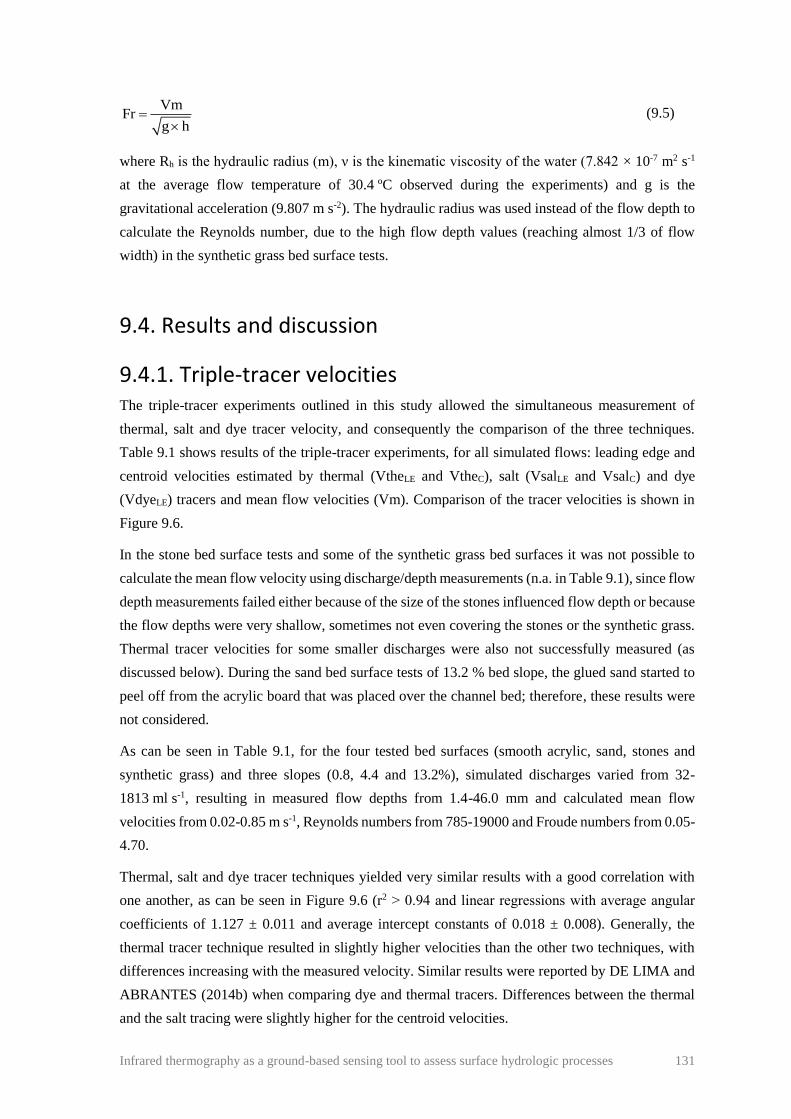
Infrared thermography as a ground-based sensing tool to assess surface hydrologic processes 131

VmFr

g h=

(9.5)

where Rh is the hydraulic radius (m), ν is the kinematic viscosity of the water (7.842 × 10-7 m2 s-1

at the average flow temperature of 30.4 ºC observed during the experiments) and g is the

gravitational acceleration (9.807 m s-2). The hydraulic radius was used instead of the flow depth to

calculate the Reynolds number, due to the high flow depth values (reaching almost 1/3 of flow

width) in the synthetic grass bed surface tests.

9.4. Results and discussion

9.4.1. Triple-tracer velocities The triple-tracer experiments outlined in this study allowed the simultaneous measurement of

thermal, salt and dye tracer velocity, and consequently the comparison of the three techniques.

Table 9.1 shows results of the triple-tracer experiments, for all simulated flows: leading edge and

centroid velocities estimated by thermal (VtheLE and VtheC), salt (VsalLE and VsalC) and dye

(VdyeLE) tracers and mean flow velocities (Vm). Comparison of the tracer velocities is shown in

Figure 9.6.

In the stone bed surface tests and some of the synthetic grass bed surfaces it was not possible to

calculate the mean flow velocity using discharge/depth measurements (n.a. in Table 9.1), since flow

depth measurements failed either because of the size of the stones influenced flow depth or because

the flow depths were very shallow, sometimes not even covering the stones or the synthetic grass.

Thermal tracer velocities for some smaller discharges were also not successfully measured (as

discussed below). During the sand bed surface tests of 13.2 % bed slope, the glued sand started to

peel off from the acrylic board that was placed over the channel bed; therefore, these results were

not considered.

As can be seen in Table 9.1, for the four tested bed surfaces (smooth acrylic, sand, stones and

synthetic grass) and three slopes (0.8, 4.4 and 13.2%), simulated discharges varied from 32-

1813 ml s-1, resulting in measured flow depths from 1.4-46.0 mm and calculated mean flow

velocities from 0.02-0.85 m s-1, Reynolds numbers from 785-19000 and Froude numbers from 0.05-

4.70.

Thermal, salt and dye tracer techniques yielded very similar results with a good correlation with

one another, as can be seen in Figure 9.6 (r2 ˃ 0.94 and linear regressions with average angular

coefficients of 1.127 ± 0.011 and average intercept constants of 0.018 ± 0.008). Generally, the

thermal tracer technique resulted in slightly higher velocities than the other two techniques, with

differences increasing with the measured velocity. Similar results were reported by DE LIMA and

ABRANTES (2014b) when comparing dye and thermal tracers. Differences between the thermal

and the salt tracing were slightly higher for the centroid velocities.

Table 9.1. Overall results of the triple tracer experiments.

Tracer velocity (m s-1)*

Slope

S (%)

Discharge

Q (ml s-1)

Mean flow

velocity

Vm (m s-1)

Thermal Salt Dye

Leading edge

VtheLE

Centroid

VtheC

Leading edge

VsalLE

Centroid

VsalC

Leading edge

VdyeLE

Sm

oo

th a

cry

lic

0.8 650 0.475 0.608 ± 0.013 0.608 ± 0.009 0.596 ± 0.033 0.547 ± 0.040 0.559 ± 0.008

0.8 856 0.516 0.703 ± 0.014 0.684 ± 0.010 0.639 ± 0.019 0.547 ± 0.047 0.629 ± 0.013

0.8 1158 0.580 0.762 ± 0.008 0.772 ± 0.020 0.637 ± 0.020 0.597 ± 0.027 0.709 ± 0.004

4.4 420 0.529 0.645 ± 0.012 0.639 ± 0.005 0.595 ± 0.043 0.552 ± 0.019 0.585 ± 0.016

4.4 696 0.623 0.828 ± 0.048 0.791 ± 0.016 0.717 ± 0.134 0.649 ± 0.071 0.715 ± 0.006

13.2 71 0.345 0.572 ± 0.058 0.378 ± 0.025 0.591 ± 0.009 0.460 ± 0.014 0.540 ± 0.015

13.2 164 0.619 0.777 ± 0.082 0.683 ± 0.015 0.725 ± 0.063 0.573 ± 0.030 0.630 ± 0.021

13.2 450 0.851 1.036 ± 0.018 0.944 ± 0.024 0.901 ± 0.095 0.945 ± 0.039 0.944 ± 0.027

San

d

0.8 47 0.035 0.092 ± 0.002 0.081 ± 0.005 0.080 ± 0.008 0.106 ± 0.003 n.a.

0.8 81 0.070 0.116 ± 0.002 0.121 ± 0.007 0.138 ± 0.001 0.108 ± 0.006 0.114 ± 0.006

0.8 210 0.079 0.172 ± 0.005 0.166 ± 0.005 0.156 ± 0.015 0.143 ± 0.009 0.163 ± 0.004

4.4 72 0.033 0.105 ± 0.002 0.102 ± 0.005 0.122 ± 0.006 0.095 ± 0.004 n.a.

4.4 259 0.178 0.332 ± 0.009 0.269 ± 0.004 0.317 ± 0.001 0.252 ± 0.002 0.343 ± 0.003

4.4 884 0.371 0.639 ± 0.017 0.530 ± 0.007 0.538 ± 0.049 0.441 ± 0.010 0.581 ± 0.028

* Tracer velocities are averages ± standard deviation of three repetitions; n.a. for not applicable (not able to measure)

Table 9.1. Overall results of the triple tracer experiments (Continuation).

Tracer velocity (m s-1)*

Slope, S

(%)

Discharge, Q

(ml s-1)

Mean flow

velocity, Vm

(m s-1)

Thermal Salt Dye

Leading edge, VtheLE Centroid, VtheC Leading edge, VsalLE Centroid, VsalC Leading edge, VdyeLE

Sto

nes

0.8 219 n.a. 0.130 ± 0.010 0.084 ± 0.009 0.117 ± 0.009 0.087 ± 0.002 0.132 ± 0.001

0.8 864 n.a. 0.359 ± 0.040 0.240 ± 0.008 0.313 ± 0.019 0.187 ± 0.003 0.277 ± 0.005

0.8 1813 n.a. 0.411 ± 0.032 0.342 ± 0.102 0.382 ± 0.088 0.288 ± 0.053 0.369 ± 0.009

4.4 256 n.a. 0.144 ± 0.004 0.099 ± 0.002 0.138 ± 0.011 0.100 ± 0.003 0.155 ± 0.007

4.4 547 n.a. 0.306 ± 0.041 0.170 ± 0.010 0.247 ± 0.007 0.167 ± 0.003 0.263 ± 0.002

4.4 1131 n.a. 0.466 ± 0.040 0.375 ± 0.015 0.398 ± 0.033 0.248 ± 0.005 0.422 ± 0.054

13.2 32 n.a. 0.059 ± 0.013 0.050 ± 0.009 0.084 ± 0.002 0.065 ± 0.001 n.a.

13.2 102 n.a. 0.092 ± 0.004 0.095 ± 0.005 0.096 ± 0.001 0.085 ± 0.001 0.088 ± 0.014

13.2 753 n.a. 0.351 ± 0.012 0.274 ± 0.005 0.374 ± 0.018 0.247 ± 0.003 0.451 ± 0.059

Sy

nth

etic

gra

ss

0.8 94 0.025 0.084 ± 0.003 0.089 ± 0.001 0.109 ± 0.002 0.052 ± 0.006 n.a.

0.8 438 0.080 0.192 ± 0.014 0.181 ± 0.006 0.225 ± 0.006 0.151 ± 0.008 0.205 ± 0.005

0.8 1067 0.156 0.338 ± 0.006 0.299 ± 0.007 0.307 ± 0.007 0.194 ± 0.025 0.255 ± 0.011

4.4 75 n.a. 0.043 ± 0.010 0.049 ± 0.005 0.072 ± 0.002 0.058 ± 0.001 n.a.

4.4 549 0.207 0.432 ± 0.009 0.312 ± 0.009 0.472 ± 0.026 0.284 ± 0.009 0.339 ± 0.014

4.4 1103 0.417 0.688 ± 0.014 0.530 ± 0.035 0.564 ± 0.030 0.371 ± 0.007 0.555 ± 0.027

13.2 52 n.a. 0.045 ± 0.002 0.036 ± 0.002 0.062 ± 0.004 0.055 ± 0.002 n.a.

13.2 202 0.118 0.175 ± 0.015 0.147 ± 0.008 0.210 ± 0.014 0.147 ± 0.007 0.239 ± 0.042

13.2 1239 0.461 0.834 ± 0.012 0.703 ± 0.075 0.752 ± 0.052 0.545 ± 0.060 0.831 ± 0.006

* Tracer velocities are averages ± standard deviation of three repetitions; n.a. for not applicable (not able to measure)

134 Infrared thermography as a ground-based sensing tool to assess surface hydrologic processes

Figure 9.6. Comparison between thermal (Vthe), salt (Vsal) and dye (Vdye) tracer velocities for

all simulated flows (subscripts LE and C stand for leading edge and centroid, respectively).

Thermal tracer velocities Figure 9.7 presents results of the thermal tracer flow velocity measurements. Two flow conditions

are shown for each tested bed surface, corresponding to the lowest and highest calculated mean

flow velocity (see Table 9.1). Two snapshots (time interval of 1 s) of the thermal videos of the

passage of the thermal tracer along the channel are shown for each flow condition.

The movement of the thermal tracer along the channel was always visible for all simulated flows;

however, whereas for higher flow velocities its movement is well defined and well-shaped

throughout the channel’s length, for lower flow velocities its movement in some cases was only

visible during the initial part of the measurement section (e.g. for stone bed surface with a discharge

of 32 ml s-1 and a 13.2% slope). This is related to the non-conservative aspect of the thermal tracer,

i.e. temperature diffusion. Lower velocities seem to result in higher temperature diffusion, which

can be seen by the dimension of the thermal marks (i.e. pixels with temperature above the threshold

value) and maximum temperature values of the tracer (TMAX in Figure 9.7) as it passes along the

channel. Overall, lower velocities have lower thermal marks and lower TMAX. Larger bed roughness

elements (e.g. stones) also induced higher tracer diffusion and lower tracer conservation, either by

the higher dissipation of flow energy or by heat transfer between flow and the rough element.

Infrared thermography as a ground-based sensing tool to assess surface hydrologic processes 135

Figure 9.7. Snapshots of the passage of the thermal tracer along the channel for two flow

conditions for each tested bed surface. S is the surface slope, Q is the discharge, VtheLE and VtheC

are the thermal tracer leading edge and centroid velocities, TMAX and TMAXt0 are the maximum and

threshold temperatures.

One aspect that should be taken into account in the previous observation is that, in general, higher

flow velocities were the result of higher discharges and therefore a higher volume of tracer, which

facilitates the conservation of the thermal tracer during its passage along the channel. However, for

lower flow velocities and lower discharges, the lower volumes of tracer did not facilitate their

conservation for the length of the channel. Therefore, one way to improve the conservation of the

thermal tracer is to increase the volume of added tracer; however, this will increase the error in

estimating the flow velocity, since larger volumes of tracer interfere with velocity, especially for

smaller discharges where the influence of the volume of added tracer would be more noticeable

(DE LIMA and ABRANTES, 2014b; DE LIMA et al., 2015b). Therefore, the optimal volume of

thermal tracer will be the smallest amount that permits the application of the technique, i.e. clear

visualization of the movement of the tracer in the flow.

An alternative to the presented methodology is to introduce a temperature sensor in the water flow

instead of using the infrared camera to detect the movement of the thermal tracer; however,

introducing a sensor in the water will perturb the flow itself and in these very shallow flows of

millimetres to a few centimetres, it is not always possible to properly measure the temperature with

a sensor, since these type of sensors usually need a minimum water depth to perform correct

measurements.

136 Infrared thermography as a ground-based sensing tool to assess surface hydrologic processes

Another way to diminish the non-conservative aspect of the thermal tracer is by reducing the

distance between the tracer addition point and the measuring section; however, this will again

increase the error in estimating the flow velocity, since the tracer addition can cause disturbances

in the flow that are more noticeable closer to the addition point and for smaller discharges. This can

be seen in Figure 9.8, which shows that estimated thermal velocities vary with the distance from

the tracer addition point. On the one hand, higher velocities closer to the tracer addition point can

be caused by the disturbance of the tracer addition, even considering the distance of 0.4 m between

the tracer addition point and the beginning of the measurement area. On the other hand, the non-

conservative aspect of the thermal tracer causes a decrease in estimated thermal velocity with

increasing distance to the tracer addition point.

The tracer temperature decreases as the distance to the tracer addition point increases and, therefore,

tracer temperature slowly dissipates in the background water temperature. This effect had more

impact on the leading edge velocity (Figure 9.8a) than on the centroid velocity (Figure 9.8b)

because the temperature dissipation occurs first in the interface between the tracer and the water.

This effect also increases as bed roughness increases and flow velocity decreases and is stronger

for the stone bed surface and weaker for the smooth acrylic bed surface (i.e. higher heat transfer

between flow and the rough element).

Figure 9.8. Thermal tracer estimated flow velocities as function of the distance to triple tracer

addition point: a) Leading edge velocity; and b) Centroid velocity. The flow velocity is presented

as a ratio between flow velocity at different locations along the length of the channel (VtheLEx and

VtheCx) and the mean flow velocity along the entire channel ( LEVthe and CVthe ).

Infrared thermography as a ground-based sensing tool to assess surface hydrologic processes 137

Another aspect to be considered when using a thermal tracer is its temperature. A higher tracer

temperature will improve the conservation of the tracer without significantly compromising

velocity measurements. In previous experiments, DE LIMA and ABRANTES (2014b) found that

the relative differences between the leading edge velocities of tracers at 15 and 85 ºC were similar

to the relative differences between tracers at the same temperature, as result of the variability

induced by the manual addition of the tracer.

Salt tracer velocities Salt transport graphs (i.e. electrical conductivity) recorded at the channel outlet for two flow

conditions and the four different tested bed surfaces are shown in Figure 9.9 (same tests presented

in Figure 9.7 for thermal tracer). For all experiments, it was always possible to detect the passage

of the salt in the outlet and therefore measure the flow velocity either by the leading edge or the

centroid. Unlike the thermal and dye tracers, the salt tracer only gave a one-off measurement of

flow velocity.

Figure 9.9. Salt transport graphs for two flow conditions for each tested bed surface: a) Higher

velocities; and b) Lower velocities. S is the surface slope, Q is the discharge, VsalLE and VsalC are

the salt tracer leading edge and centroid velocities, EC is the electrical conductivity and ECMAX5s

is the threshold electrical conductivity.

In general, higher mean velocities (see Table 9.1) lead to an earlier rise and peak of the salt transport

graph, resulting in higher leading edge (VsalLE) and centroid velocities (VsalC). As the estimated

salt velocities increased, so did the salt transport peak, while the base transport time (i.e. time from

138 Infrared thermography as a ground-based sensing tool to assess surface hydrologic processes

the initial rise in conductivity above the threshold value to the decay below the threshold value)

decreased.

The relation between the estimated salt velocities (VsalLE and VsalC) and the total mass of salt

transported by the flow, presented as a ratio of the total mass of salt detected by the electrical

conductivity sensor at the channel outlet (Mtransp) to the total mass of salt added to the flow (Madded),

is shown in Figure 9.10. Similar to the thermal tracer, the non-conservative aspect of the salt tracer

decreases with flow velocity, since salt transport increases. A major concern when using salt tracers

to measure flow velocity is how to ensure that the salt is completely dissolved in the flow so that it

can be properly detected (DAY, 1977). In the present study, salt was added as an aqueous solution

with hot water, which greatly helped the salt to mix in the flow. Therefore, the decrease of salt

transport with lower flow velocity would be closely related to the bed surface roughness. In fact,

the average ratio of salt transport for the different tested bed surfaces was 1.02 ± 0.07, 0.85 ± 0.13,

0.87 ± 0.13 and 0.74 ± 0.30 for the smooth acrylic, sand, stones and synthetic grass, respectively.

Figure 9.10. Relation between estimated leading edge and centroid salt velocities (VsalLE and

VsalC) and the ratio between mass of transported (Mtransp) and added (Madded) salt. Vertical bars

indicate standard deviation.

One way to improve the conservation of the salt tracer is to increase salt concentration and decrease

the distance from the tracer addition point to the sampling point. It should be noted, however, that,

similar to the thermal tracer, salt tracer velocities tend to decrease with increasing distance from

the salt addition point (CALKINS and DUNNE, 1970; PLANCHON et al., 2005). At the same time,

higher salt concentration would need a longer mixing time to ensure the salt is properly dissolved

in the flow. Therefore, when using a salt tracer, the salt solubility, concentration, addition method

(e.g. dry or as an aqueous solution), flow conditions (e.g. discharge, depth, velocity), bed surface

roughness and mixing length must all be taken into consideration.

Dye tracer velocities Figure 9.11 presents the results of the dye tracer flow velocity measurements (same tests presented

in Figures 9.7 and 9.9 for thermal and salt tracers, respectively). Two snapshots of the real image

Infrared thermography as a ground-based sensing tool to assess surface hydrologic processes 139

videos of the dye tracer passing along the 0.5 m measuring section (Section 2 in Figure 9.5) are

shown for each flow condition.

It was not always possible to estimate flow velocity with the dye tracer for the tested flow

conditions. This was because for lower discharges, and thus for lower volumes of added tracer, the

dye tracer could not be visualized as it passed along the channel (see Figure 9.11 and n.a. in

Table 9.1). This is related to the non-conservative aspect of the dye tracer and, as with the thermal

and salt tracers, it was more evident for lower flow velocities in the higher bed surface roughness

tests.

Figure 9.11. Photographs of the passage of the dye tracer in a measuring section (Section 2 in

Figure 9.5) for two flow conditions for each tested bed surface. S is the surface slope, Q is the

discharge, VdyeLE is the dye leading edge velocity, Δx is the measuring section length and Δt is

the time interval.

One way to increase the conservation of the dye tracer is to increase the dye concentration and

decrease the distance from the tracer addition point to the sampling point. But as with the thermal

and salt tracers, the dye tracer leading edge flow velocity decreases with increasing distance from

the tracer addition point (Figure 9.12). Furthermore, timing errors, unavoidable due to human

reaction time and the frame rate of the recording system, will tend to increase with shorter

measurement lengths (DE LIMA and ABRANTES, 2014b; DUNKERLEY, 2003). Other way to

improve dye tracing performance is to use an automated mechanism of detecting the passage of the

dye tracer such as the ones used in DUNKERLEY (2003) and HOLDEN et al. (2008).

140 Infrared thermography as a ground-based sensing tool to assess surface hydrologic processes

Figure 9.12. Ratio between dye tracer leading edge velocities for the three measuring sections

(VdyeLESection) and the mean dye tracer velocity along the entire channel (VdyeLE).

9.4.2. Advantages and disadvantages of the tracer techniques Overall, the main advantages of the thermal tracer technique over the dye tracer technique were:

i) Higher visibility of the tracer in the thermal videos compared with the real image videos;

ii) Estimation of flow velocities using smaller volume of tracer, and, therefore, smaller disturbances

in the actual flow velocity; and iii) Easy estimation of centroid velocities that are very difficult to

obtain from dye tracer measurements, since they require more sophisticated image processing and

specific light conditions that may not be always available, especially in field tests. The main

advantages of the thermal tracer technique over the salt tracer technique were: i) The visualization

of the movement of the thermal tracer along the measuring section; ii) The possibility of measuring

space-averaged flow velocities using only one infrared video camera instead of only one velocity

value using only one electrolyte sensor (space-averaged salt tracer velocities would require multiple

sensors placed along the flume); iii) The possibility of measuring the flow velocity without the need

of introducing any instrument (sensor) in the flow, causing less disturbances in the actual flow

velocity; and iv) The non-necessity of a minimum water depth, which usually is needed to

accurately measure the salt concentration with an electrolyte sensor. The thermal tracer also offers

a cleaner and more ecologically friendly way of measuring in situ flow velocities than the dye and

salt tracers do, since it leaves no residue in the water or the soil and causes very little temporal and

spatial disturbance to the environment.

Overall, the main disadvantages of the thermal tracer technique over the dye and salt tracers

techniques were: i) High price of an infrared video camera compared with a regular optical video

camera or an electrolyte sensor, despite recent falls in the cost of infrared equipment; and ii) The

need to have an energy source to heat or cool the water rather than simply having to add colouring

or salt might be an obstacle, especially in remote field studies. The thermal tracer showed less

conservation in the flow than the salt tracer and the accuracy of the measurement seemed to depend

more on the volume and/or temperature of the tracer than on the concentration of the salt. Measuring

Infrared thermography as a ground-based sensing tool to assess surface hydrologic processes 141

flow velocity using the dye tracer can be faster and more intuitive than the thermal tracer, since the

movement of the tracer can be simply observed by the operator without using any recording

equipment (e.g. camera, sensor), which can be especially useful in field applications.

9.4.3. α and β correction factors Figure 9.13 presents the comparison between mean flow velocities (Vm) calculated from flow

discharge/depth measurements and the leading edge and centroid velocities measured with the

triple-tracer technique. Results of the stone bed surface tests were not considered, since it was not

possible to calculate mean flow velocity.

Leading edge and centroid tracer velocities presented a good correlation with mean flow velocity

(r2 ˃ 0.89 in Figure 9.13). As expected, tracer velocities were higher than mean flow velocity, with

higher values for the leading edge. In fact, as stated before, leading edge is regarded as the surface

velocity of the flow, i.e. the theoretical maximum (or near maximum) value of the flow velocity

profile. In turn, centroid velocity is regarded as the theoretical mean value of the flow velocity

profile, if conservation of the tracer in the flow is assumed. However, since none of the tracers

exhibited absolute conservation during the experiments, centroid velocities were slightly higher

than mean flow velocity.

Figure 9.13. Comparison between mean flow velocities (Vm) and thermal (Vthe), salt (Vsal) and

dye (Vdye) tracer velocities for all simulated flows (subscripts LE and C stand for leading edge

and centroid, respectively).

Since tracer velocities were higher than mean flow velocity, a correction factor must be used to

convert the measured tracer velocities into actual mean flow velocities. In this study, two correction

factors were considered: i) α as the ratio between the mean flow velocity (Vm) and the leading edge

velocity measured by means of the triple-tracer technique (VtheLE, VsalLE and VdyeLE); and ii) β as

the ratio between the mean flow velocity (Vm) and the centroid velocity, measured by means of

thermal and salt tracers (VtheC and VsalC). Thermal, salt and dye tracer correction factors α and β

142 Infrared thermography as a ground-based sensing tool to assess surface hydrologic processes

calculated for the smooth acrylic, sand and synthetic grass (stone bed surface results were not

considered) are shown in Figure 9.14. As can be seen, there are no significant differences in the α

and β values for the tracer techniques. Thermal, salt and dye α correction factors ranged from 0.283-

0.879, 0.225-1.034 and 0.277-1.017 with average values of 0.595 ± 0.166, 0.626 ± 0.219 and

0.676 ± 0.193, respectively. Thermal and salt β correction factors ranged from 0.274-0.967 and

0.320-1.149 with average values of 0.666 ± 0.187 and 0.774 ± 0.223, respectively.

Figure 9.14. Correction factors derived from the triple-tracer experiments, for the smooth acrylic,

sand and synthetic grass bed surfaces: a) α; and b) β. Columns with the same lowercase letter do

not differ significantly for Tukey’s test (p ˂ 0.05).

The observed range of α included Horton’s theoretical value of 0.67 for an infinitely wide, perfect

laminar flow on a smooth and immobile bed (HORTON et al., 1934) and the α lower boundary of

0.225 agrees with the range of approximately 0.2-0.9 found in previous studies (DUNKERLEY,

2001; EMMETT, 1970; LI and ABRAHAMS, 1997; LI et al., 1996; PLANCHON et al., 2005;

ZHANG et al., 2010); however, the upper boundary was higher (1.034). For all simulated flows,

observed β values were higher than the α values, which is in line with the theory that tracer centroid

velocities are mean theoretical velocities, if conservation of the tracer is assumed. Lower and upper

boundaries of β (0.274-1.149) exceeded the range of 0.7-0.9 observed by LI et al. (1996) and 0.6-

1.0 observed by PLANCHON et al. (2005). However, all previous studies presented a broad variety

of findings and conclusions, without actually defining fixed conversion factors or relations. In fact,

the variation of α and β is the result of a very complex relation between the shape of the flow

velocity profile and the flow characteristics (e.g. velocity, depth, Reynolds number, Froude

number) and the bed surface characteristics (e.g. roughness, slope).

Infrared thermography as a ground-based sensing tool to assess surface hydrologic processes 143

As shown in Figure 9.14, significant differences were found for α and β (the latter to a lesser extent)

between the smooth acrylic bed surface and the rough bed surfaces (sand and synthetic grass), with

α and β being smaller for the rough bed surfaces. These findings are in agreement with EMMETT

(1970) who found smaller α in field experiments than in laboratory experiments, since natural field

soil surfaces had a wider range of roughness elements than the laboratory sand surfaces. Roughness

elements will perturb the flow and give rise to steeper velocity profiles with a wider gap between

the flow velocity profile mean and maximum (i.e. flow surface velocity) values, which implies

lower α values. DUNKERLEY (2001) also observed a tenuous inverse relation between roughness

and α.

Correction factors increased with increasing Reynolds number (Re) and Froude number (Fr), as

shown in Figure 9.15. Here, only thermal correction factors are presented, though it should be noted

that salt and dye correction factors showed similar behaviour. An increase in Re and Fr increases

flow turbulence and flow speed, which results in a better mixing of the flow, and a less steep

velocity profile, approaching the flow velocity profile mean and maximum values. Therefore, a

smaller correction of the tracer velocities is required (i.e. correction factors closer to 1).

The variation of α and β with Re reported in previous studies largely depends on the studied flow

regime (i.e. range of Re). EMMETT (1970) found lower values of α for laminar flow (Re ˂ 2000),

which increased during transitional flow (Re between 2000-8000), with the highest being for

turbulent flow (Re ˃ 8000). LI et al. (1996) observed an increase of α and β with Re in the

transitional flow regime. LI and ABRAHAMS (1997) observed lower values of α in laminar flow,

without a distinct trend with Re, a steep rise of α in the transitional flow and a slight rise in the

turbulent range. DUNKERLEY (2001), too, did not find any relation between α and Re in the

subcritical laminar range (Re between 100-500). In the present study, the variation of α and β with

Re was tenuous (power regressions with r2 of 0.26 and 0.29 in Figure 9.15a) and no clear distinction

could be made between the different bed surfaces and the different flow regimes, thus the best fit

was achieved when all data was plotted together. Only a slight distinction was found between a rise

in the laminar and transitional phase (Re ˂ 8000) and a slight decrease during the turbulent phase

(Re ˃ 8000). The rise in the laminar and transitional phase, without any distinction between them,

was also noted in ZHANG et al. (2010). The slight decrease during the turbulent phase has not been

reported in previous studies, but the highest Re studied previously was 13000 in LI and

ABRAHAMS (1997) and LI et al. (1996) whereas in the present study a maximum of 19000 was

reached.

In the present study, a stronger correlation was found with the variation of α and β with the Froude

number. Here, the variation of Fr was closely related to the roughness of the surface of the bed; on

the smooth acrylic bed surface the flow was supercritical (Fr ˃ 1), with Fr between 1.60-4.70, and

on the sand and synthetic grass surfaces the flow varied from subcritical (Fr ˂ 1) to critical (Fr ≈ 1),

with Fr between 0.05-1.09 (Figure 9.15b). As stated before, higher roughness leads to lower

correction factors. The variation of α and β with Fr, was also observed previously in LI and

144 Infrared thermography as a ground-based sensing tool to assess surface hydrologic processes

ABRAHAMS (1997) with Fr varying between 0.4-3.2. Such relations were not clear in other

studies, e.g. LI et al. (1996) and ZHANG et al. (2010) only studied critical to supercritical flow,

and DUNKERLEY (2001) only studied subcritical flow.

Variation of the correction factors with flow velocity, flow depth and bed slope was further

analysed. The correction factors α and β both increased with flow velocity regardless of the flow

regime, as shown in Figure 9.16, since these variations were similar for the laminar and turbulent

flow and for the subcritical and supercritical flow. Best fit was thus achieved when all data were

plotted together. Similar results have been reported in the literature (DUNKERLEY, 2001;

EMMETT, 1970; LI and ABRAHAMS, 1997; LI et al., 1996; PLANCHON et al., 2005; ZHANG

et al., 2010).

Figure 9.15. Variation of thermal α and β with: a) Reynolds number; and b) Froude number.

Figure 9.16. Variation of thermal α and β with mean flow velocity (Vm).

Infrared thermography as a ground-based sensing tool to assess surface hydrologic processes 145

The variation of α with flow depth and bed slope is shown in Figures 9.17 and 9.18. Here, only α

is presented, though it should be noted that β showed similar behaviour. These variations depended

on the flow regime, since they differed between the laminar and transitional plus turbulent flow.

No differences were observed between subcritical and supercritical flow, however. Therefore, best

fit was achieved when laminar and transitional plus turbulent data were plotted separately, has

shown in Figure 9.17. In Figure 9.18 data was plotted separately by surface bed. In this situation,

best fit was achieved when transitional plus turbulent data was plotted individually. When

separating data by bed surface, no clear relation was observed for laminar flow.

In the present study, α decreased with flow depth; this can be attributed to lower flow velocities

observed for the rough surfaces that had the higher flow depths. As stated before, higher roughness

leads to lower correction factors. The decrease in α with flow depth was also described in

DUNKERLEY (2001) and in LI and ABRAHAMS (1997) for laminar flow. However, in LI and

ABRAHAMS (1997), LI et al. (1996) and ZHANG et al. (2010) an increase of α with flow depth

for transactional and turbulent flow was observed. Each of the three previous studies used only one

type of bed surface: smooth acrylic bed surface in LI et al. (1996), and sand bed surface in LI and

ABRAHAMS (1997) and ZHANG et al. (2010). In the present study, an increase of α with flow

depth was only observed for transitional flow on the sand bed surface, as shown in Figure 9.18a. In

this case, as stated by ZHANG et al. (2010), the influence of grain roughness on flow velocity

profile may decrease as flow depth increases, resulting in smoother velocity profiles.

Figure 9.17. Graphs for α for laminar and turbulent flows, against: a) Flow depth; and b) Bed

slope. Turbulent flow includes the transitional phase (Re ˃ 2000).

146 Infrared thermography as a ground-based sensing tool to assess surface hydrologic processes

The variation of α with bed slope varied considerably with flow regime; while no clear relation was

observed for turbulent flow, for laminar flow there was a positive logarithmic relation with good

correlation (r2 = 0.86). Therefore, slope played an important role in controlling the shape of the

flow velocity profile in the laminar range. In fact, for a given flow discharge, as slope gradient

increased so did flow velocity, and flow depth decreased.

Figure 9.18. Graphs for α observed for the turbulent flows in the different bed surfaces, against: a)

Flow depth; and b) Bed slope. Turbulent flow includes the transitional phase (Re ˃ 2000).

As shown before, an increase in flow velocity results in higher α values. Previous studies had

different results; in LI et al. (1996) and ZHANG et al. (2010), α decreased with slope for transitional

and turbulent flow, but in LI and ABRAHAMS (1997) α did not vary with slope for laminar,

transitional or turbulent flow. However, it should be remembered that only one type of bed surface

was used in these studies. In the present study, a decrease of α with bed slope was only observed

for transitional flow on the sand bed surface, as shown in Figure 9.18b.

Infrared thermography as a ground-based sensing tool to assess surface hydrologic processes 147

9.5. Conclusions

To better understand and model the dynamics of sediment and pollutant transport by overland flow,

flow velocities must be measured. Traditional dye and salt tracer techniques and the more recent

thermal tracer technique have been used to measure flow velocity, especially in shallow muddy

overland flows in the field. In this study, a novel triple-tracer approach was tested, using dyed-

salted-heated water. This novel approach gave insight into the measurement of shallow flow

velocities and proved to be a useful tool to compare the three techniques. However, it is worth

mentioning that despite the improvement achieved by using this triple-tracer approach, many

difficulties remained in evaluating shallow flow velocity measurements because of the complexity

and spatial and temporal variability of shallow flow. Also, the simultaneous addition of the three

tracers may limit each other to their best measurement precisions and the effect of the heated water

on dye and salt and vice-versa, although presumably minimal, is not fully known.

Results showed that thermal tracing can be used to estimate shallow flow velocities, since the results

are similar to those given by other traditional and well-established flow velocity measurement

techniques, such as dye and salt tracing. In general, thermal tracer velocities were slightly higher,

followed by dye and salt tracer velocities; however, no significant differences were observed

between them.

In these triple-tracer experiments, the volume of added tracer was one of the most important limiting

factors of the thermal and dye tracer techniques, whereas for the salt tracer this limitation was not

so noticeable. It should be noticed that, the ideal volume for each tracer should be different and,

therefore, the triple-tracer approach may has conditioned the best performance of each method.

However, it is also true that the optimal volume of tracer should be the smallest amount that creates

the smallest disturbance to the actual flow velocity and, at the same time, permits its clear

visualization. In this case, the dye tracer was the less successful technique, since for some lower

discharges and lower volumes of added tracer it was not always possible to estimate flow velocity

with the dye tracer.

For field applications, the dye tracer technique seems to be faster and simpler, especially if only in

situ visual observation is performed (i.e. no recording device). However, the involvement of human

perception and reaction time is more prone to timing errors. If an optical video camera is used, the

operator should ensure that light conditions are suitable to post imaging analyses, especially if the

centroid velocity of the dye tracer is to be measured. For large scale field applications (e.g. hillslope

scale) the salt tracer seems to be more appropriate due to the higher conservation. However, the

movement of the salt tracer along the measuring section and the possibility of measuring space-

averaged flow velocities can only be achieved by installing multiple sensors, which can ultimately

cause higher disturbance to the actual flow velocity. Also, many sensors require a minimum water

depth that may not be available during shallow flow monitoring. Thermal tracer allows to clearly

visualise the movement of the tracer along the measuring section with high accuracy. However, it

148 Infrared thermography as a ground-based sensing tool to assess surface hydrologic processes

requires more expensive equipment (i.e. infrared video camera) and an energy source to heat the

tracer.

The results showed that the correction factors used to estimate the mean velocity of overland flow

from the tracer’s leading edge and centroid velocity measurements depend on the flow regime,

since they increased with higher Reynolds and Froude numbers. In this study, the correction factors

varied directly with flow velocity and slope and inversely with flow depth and bed roughness. In

soil erosion and solute transport studies these variables greatly vary in space and time, especially

in the field. Therefore, velocity estimation from tracers involves a large amount of uncertainty and

caution is required when using these measurements. Data presented in this study can provide new

insights on correction factors used in tracing velocity estimation, which is a field not yet clearly

understood.

Clear flowing water was used in this study. Further studies are therefore required to investigate the

effect of sediment load on the thermal tracer performance and on the respective correction factors.

Also, to achieve the best calibration of the thermal tracer technique, further tests should be

conducted using different volumes of tracer at different temperatures (hotter and colder water than

the flow) and different measuring sections.

“Research always takes three times longer than planned, even after taking this rule into

account.”

- Unknown

Infrared thermography as a ground-based sensing tool to assess surface hydrologic processes 151

10. COMBINING A THERMAL TRACER WITH A TRANSPORT MODEL TO ESTIMATE SHALLOW FLOW VELOCITIES8

10.1. Abstract

For a long time, tracer techniques based on dyes, salts and more recently heat have been used to

estimate shallow flow velocities. Traditionally, flow velocity estimation using tracers would consist

of tracking the movement of the leading edge or the centroid of the tracer with the flow. An

alternative methodology uses an analytical solution of an advection–dispersion transport equation

as the mathematical foundation for measuring shallow water flow velocity from tracer

measurements.

The main goal of the present study was to ascertain whether this alternative numerical methodology

can be used with temperature data from thermal tracer measurements. Salt and thermal tracer

techniques were applied simultaneously by injecting a double tracer of salted-heated water into

different shallow flows simulated in a laboratory hydraulic flume. Simulated flows combined

different bed surfaces (smooth acrylic sheet, rough sand board and synthetic grass carpet), flow

discharges (from 47 to 1239 ml s-1) and bed slopes (0.8, 4.4 and 13.2%), resulting in a wide range

of hydraulic conditions. Velocities determined with the abovementioned methodology were

compared with those estimated by measuring the tracers’ leading edge and centroid and with mean

flow velocity calculated using discharge/depth measurements.

Results from combining this alternative numerical methodology with thermal tracer data were

similar to results from the salt tracer. Also, the proposed alternative numerical methodology

predicted the mean flow velocity calculated from discharge/depth measurements better than the

measurements of the leading edge and centroid of the tracers.

Keywords Thermal tracer; Salt tracer; Advection-dispersion transport equation; Shallow flow velocity;

Hydraulic flume

8 ABRANTES, J.R.C.B., MORUZZI, R.B., DE LIMA, J.L.M.P., SILVEIRA, A. and MONTENEGRO,

A.A.A. (2019). Combining a thermal tracer with a transport model to estimate shallow flow velocities.

Physics and Chemistry of the Earth, 109, 59-69. DOI:10.1016/j.pce.2018.12.005.

152 Infrared thermography as a ground-based sensing tool to assess surface hydrologic processes

10.2. Introduction

Shallow flows can occur in natural and urbanised basins (e.g. hillslopes, drainage systems) and the

accurate measurement of their velocity has been of great concern to hydro-environmental

researchers since it would help to better understand and model the dynamics of sediment and

pollutant transport.

For a long time, tracer techniques have been used to estimate flow velocity. Many people regard

them as crude methods compared with far more sophisticated and accurate methods, such as those

based on acoustic and ultrasonic technologies (e.g. ADV, ACDP). However, those technologies

may have some limitations if used outside their ideal measurement conditions, and therefore they

cannot always be used, particularly in the case of very shallow flows with depths of millimetres to

a few centimetres. The most common materials used as tracers in flow velocity estimation are dyes

(e.g. ABRAHAMS et al., 1986; DUNKERLEY, 2003; FLURY and FLÜHLER, 1993; HOLDEN

et al., 2008; TAZIOLI, 2011) and salts (e.g. CALKINS and DUNNE, 1970; COMINA et al., 2014;

COMITI et al., 2007; DAY, 1977; TATARD et al., 2008). The movement of the dye with the flow

can be seen with the naked eye or using optical recording equipment. The passage of the salt can

be detected by an electrical conductivity sensor placed in contact with the flow.

A more recent approach in flow velocity measurement uses thermal tracers (e.g. hot water, ice

cubes) that can be detected by an infrared camera (ABRANTES et al., 2018a; DE LIMA and

ABRANTES, 2014b; DE LIMA et al., 2015b, 2018; SCHUETZ et al., 2012; TAURO and

GRIMALDI, 2017). Results show that thermal tracers can be used to estimate shallow flow

velocities, since the results are similar to those given by other traditional and well-established flow

velocity measurement techniques, such as dye tracers (ABRANTES et al., 2018a; DE LIMA and

ABRANTES, 2014b), salt tracers (ABRANTES et al., 2018a; SCHUETZ et al., 2012), current flow

meters (TAURO and GRIMALDI, 2017) and ADV equipment (DE LIMA et al., 2015b). One

advantage of thermal tracers is that the tracer is more visible in the thermal images than the dye

tracer is in the optical images. Thermal tracers can be especially useful when vegetation is

concealing the measuring area. Another advantage is the possibility of measuring space-averaged

flow velocity, which for salt tracers can only be achieved by installing multiple sensors. Some

disadvantages of thermal tracers are the equipment costs and tracer handling. Also, thermal tracers

have been shown to be less conservative than salt tracers, which can be important for large scale

field applications (e.g. hillslope scale).

Traditionally, flow velocity estimation using tracers would involve measuring the time from the

injection of the tracer to its arrival at a sampling point and then dividing this figure by the travel

distance. With dyes, the velocity of the leading edge is usually measured. With salts, either the

leading edge or centroid of the tracer’s concentration at the sampling point is usually measured.

The leading edge is regarded as the surface flow velocity and the centroid is regarded as the mean

theoretical flow velocity. However, the non-conservative aspects of the tracers, such as advection

and diffusion processes, infiltration and constant exchanges between the soil surface and water

Infrared thermography as a ground-based sensing tool to assess surface hydrologic processes 153

flow, mean that none of the measured velocities can be considered the actual mean flow velocity.

Therefore, correction factors have to be applied to obtain the mean flow velocity (HORTON et al.,

1934). Such correction factors vary with the flow characteristics (e.g. velocity, depth, regime) and

bed surface characteristics (e.g. slope, roughness), as studied in ABRANTES et al. (2018a),

DUNKERLEY (2001), EMMETT (1970), LI and ABRAHAMS (1997), LI et al. (1996),

PLANCHON et al. (2005) and ZHANG et al. (2010).

An alternative methodology for determining shallow flow velocities based on the advection-

dispersion solute transport model was proposed in LEI et al. (2005). This numerical technique

consists of fitting the analytical solution of the differential equation for solute transport in shallow

flows to solute transport data obtained by means of a salt tracer, i.e. the solute is a salt and its

transport in flow is detected by means of electrical conductivity sensors. This fitting is done by

minimising the sum of squared errors between modelled and experimentally observed data. This

method has been used in a number of studies involving the determination of shallow flow velocity

(BAN et al., 2016; CHEN et al., 2017; HUANG et al., 2018; LEI et al., 2010, 2013; RAHMA et

al., 2013; SHI et al., 2012, 2016; ZHUANG et al., 2018); it estimates flow velocity more accurately

and shows high stability relative to more traditional tracer techniques (e.g. measuring the leading

edge or centroid of the tracer). This methodology takes into account the physical processes of

advective transport caused by the shifting of the solute field (i.e. concentrated particles) due to the

flow movement and diffusive transport by which solute from particles of higher concentration is

transferred to particles of lower concentration that are in physical contact (Flick’s law).

The main goal of the present study was to ascertain whether the numerical methodology proposed

in LEI et al. (2005) could be adapted to temperature data obtained from thermal tracer experiments,

first shown in ABRANTES et al. (2018a). In fact, as with solute transport, heat transport in flowing

water is governed by advective transport caused by the translation of the energy field (i.e. heated

particles) as result of the flow movement and diffusive transport due to the transfer of energy from

higher temperature particles to lower temperature particles that are in physical contact

(Fourier's law). Therefore, heat transport in flowing water can be described using a differential

transport equation that takes both diffusive and advective transport into account, such as the one

used for solute transport.

The analogy of comparison between solute and heat transport has been made in previous

investigations. SCHUETZ et al. (2012) used thermal imaging and injections of heated-salted water

as an artificial tracer method to experimentally characterise the spatial distribution of flow paths

and to assess solute transport properties in shallow water in a constructed wetland. They found that,

at relatively small temporal and spatial scales, heated water can be regarded as a conservative tracer

with similar behaviour to salt tracer, and it allows the quantitative determination of transport

parameters such as flow velocity and hydrodynamic dispersion. Comparing salt and thermal tracer

techniques, ABRANTES et al. (2018a) observed that, for a small measuring section, the transport

of heat and solute was similar and differences between the two tracers were insignificant. The

154 Infrared thermography as a ground-based sensing tool to assess surface hydrologic processes

studies by ABRANTES et al. (2018a) and SCHUETZ et al. (2012) show that differences between

the salt and thermal tracers’ conservative properties are of the same magnitude as method errors

(e.g. different response times of the equipment , different measurement temporal frequency of the

equipment, differences between initial tracer temperature and concentration).

Numerical studies of solute and heat transport in saturated porous media (i.e. groundwater flow)

were performed by e.g. de MARSILY (1986), RAU et al. (2012) and VANDENBOHEDE et al.

(2009). Here, the same advection-dispersion transport model was used for both solute and heat

transport. Differences between solute and heat transport are simulated by the hydrodynamic and

thermal dispersion coefficients that represent both advective and diffusive transport mechanisms.

In these situations (i.e. groundwater flow in porous media) the similarity between heat and solute

transport is an approximation that may lack some precision because mass diffusion is orders of

magnitude greater in water than in minerals, whereas thermal diffusion is comparable in the two

media. However, in the present study, a single medium is considered (i.e. surface shallow flowing

water) and therefore differences between media are not important. Furthermore, in such shallow

flowing water with high flow rates, solute and heat transport processes are advection dominated

(i.e. the effect of the mechanical advection greatly exceeds that of the molecular diffusion), and

hydrodynamic and thermal dispersivity coefficients due to advection are considered to be

approximately equal.

For the purpose of this study, the analytical solution of the differential advection-dispersion

transport equation in shallow flows was fitted both to electrical conductivity data obtained with an

electrical conductivity sensor (salt tracer technique) and to temperature data obtained with an

infrared video camera (thermal tracer technique). The tracer techniques were applied

simultaneously by injecting a double tracer of salted-heated water into different shallow flows

simulated in a laboratory hydraulic flume. Simulated flows combined different bed surfaces

(smooth acrylic sheet, rough sand board and synthetic grass carpet), flow discharges (from 47 to

1239 ml s-1) and bed slopes (0.8, 4.4 and 13.2%), resulting in a wide range of hydraulic conditions.

Velocities determined with the abovementioned methodology were compared with those estimated

from measuring the tracers’ leading edge and centroid and with mean flow velocity calculated using

discharge/depth measurements.

With this adapted methodology the authors seek to combine the advantages of the thermal tracers

shown in ABRANTES et al. (2018a), DE LIMA and ABRANTES (2014b), DE LIMA et al.

(2015b), SCHUETZ et al. (2012) and TAURO and GRIMALDI (2017) with the advantages of the

numerical methodology proposed in LEI et al. (2005).

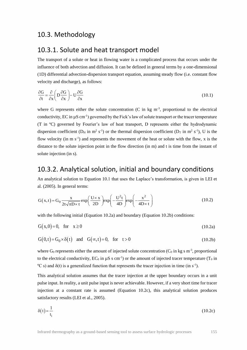
Infrared thermography as a ground-based sensing tool to assess surface hydrologic processes 155

10.3. Methodology

10.3.1. Solute and heat transport model The transport of a solute or heat in flowing water is a complicated process that occurs under the

influence of both advection and diffusion. It can be defined in general terms by a one-dimensional

(1D) differential advection-dispersion transport equation, assuming steady flow (i.e. constant flow

velocity and discharge), as follows:

G G GD U

t x x x

= −

(10.1)

where G represents either the solute concentration (C in kg m-3, proportional to the electrical

conductivity, EC in µS cm-1) governed by the Fick’s law of solute transport or the tracer temperature

(T in ºC) governed by Fourier’s law of heat transport, D represents either the hydrodynamic

dispersion coefficient (DH in m2 s-1) or the thermal dispersion coefficient (DT in m2 s-1), U is the

flow velocity (in m s-1) and represents the movement of the heat or solute with the flow, x is the

distance to the solute injection point in the flow direction (in m) and t is time from the instant of

solute injection (in s).

10.3.2. Analytical solution, initial and boundary conditions An analytical solution to Equation 10.1 that uses the Laplace’s transformation, is given in LEI et

al. (2005). In general terms:

( )2 2

0

x U x U t xG x, t G exp exp exp

2D 4D 4D t2t D t

= − −

(10.2)

with the following initial (Equation 10.2a) and boundary (Equation 10.2b) conditions:

( )G x,0 0, for x 0= (10.2a)

( ) ( ) ( )0G 0,t G t and G ,t 0, for t 0= = (10.2b)

where G0 represents either the amount of injected solute concentration (C0 in kg s m-3, proportional

to the electrical conductivity, EC0 in µS s cm-1) or the amount of injected tracer temperature (T0 in

ºC s) and δ(t) is a generalized function that represents the tracer injection in time (in s-1).

This analytical solution assumes that the tracer injection at the upper boundary occurs in a unit

pulse input. In reality, a unit pulse input is never achievable. However, if a very short time for tracer

injection at a constant rate is assumed (Equation 10.2c), this analytical solution produces

satisfactory results (LEI et al., 2005).

( )i

1t

t = (10.2c)

156 Infrared thermography as a ground-based sensing tool to assess surface hydrologic processes

where ti is the time for tracer injection (in s-1).

If conservation of the tracers in the flowing water is assumed, G0 can be calculated as the integral

area of the measured electrical conductivity or temperature curves with time (Equation 10.3).

However, since both tracers are not fully conservative, this is only an approximation of the real

value of G0.

( )0 0G G x, t dt

= (10.3)

Therefore, in this generalised analytical solution, two parameters need to be determined to describe

the transport of a solute or heat in the flow, i.e. DH and U in the case of solute transport and DT and

U in the case of heat transport. They can be determined by fitting the analytical solution to solute

or heat transport data obtained experimentally. For this purpose, solute transport data obtained with

an electrical conductivity sensor and temperature data obtained with an infrared video camera from

combined salt and thermal tracer experiments, described in ABRANTES et al. (2018a), were used.

10.4. Experimental methodology

10.4.1. Setup and simulated flows The 3.00 m long by 0.15 m wide hydraulic flume (Figure 10.1) was used to simulate flows in this

study. The flume uses a water recirculation circuit with a 500 L reservoir, a pump and a flow control

valve. The setup allows the manual adjustment of the bed slope. The flume has free inflow and

outflow and so flow velocity and depth are controlled by the flow discharge, bed slope and bed

surface roughness.

A total of 23 different flow conditions (velocities) were simulated, involving three bed surfaces

(smooth acrylic sheet, rough sand board and synthetic grass carpet), three bed slopes (0.8, 4.4 and

13.2%) and different flow discharges (between 47-1239 ml s-1), as summarised in Table 10.1.

Smooth acrylic simulations were performed on the bed’s smooth acrylic sheet. For the rough sand

simulations, ˂ 1.2 mm sieved sand particles were glued to an acrylic board that was fixed to the

flume bed. For the synthetic grass simulations, an 8.5 mm thick synthetic grass carpet was fixed to

the flume bed. Photographs, from above, of the three bed surfaces used in the experiments are

shown in Figure 10.2.

For each simulated flow, flow depth was measured using a point gauge (Figure 10.1a) and flow

discharge was measured at the flume outlet by the volumetric method.

Infrared thermography as a ground-based sensing tool to assess surface hydrologic processes 157

Figure 10.1. Schematic representation of the laboratory setup used in the experiments: a) Side

view (not to scale); b) View from above (to scale).

Figure 10.2. Photographs of the three bed surfaces used in the experiments: a) Smooth acrylic

sheet; b) Rough sand board; and c) Synthetic grass carpet. View from above, without flowing

water (left) and side view with flowing water (right).

158 Infrared thermography as a ground-based sensing tool to assess surface hydrologic processes

Table 10.1. Simulated flows.

Flow simulation S (%) Q (10-6 m3 s-1) h (10-3 m) UM (m s-1)

Smooth acrylic sheet

Acrylic_1 0.8 650 9.12 0.475

Acrylic_2 0.8 856 11.06 0.516

Acrylic_3 0.8 1158 13.31 0.580

Acrylic_4 4.4 420 5.29 0.529

Acrylic_5 4.4 696 7.45 0.623

Acrylic_6 13.2 71 1.37 0.345

Acrylic_7 13.2 164 1.77 0.619

Acrylic_8 13.2 450 3.5 0.851

Rough sand board

Sand_1 0.8 47 8.95 0.035

Sand_2 0.8 81 7.71 0.070

Sand_3 0.8 210 17.72 0.079

Sand_4 4.4 72 14.55 0.033

Sand_5 4.4 259 9.70 0.178

Sand_6 4.4 884 15.89 0.371

Synthetic grass carpet

Grass_1 0.8 94 25.07 0.025

Grass_2 0.8 438 36.50 0.080

Grass_3 0.8 1067 45.60 0.156

Grass_4 4.4 75 n.a.m. n.a.m.

Grass_5 4.4 549 17.68 0.207

Grass_6 4.4 1103 17.63 0.417

Grass_7 13.2 52 n.a.m. n.a.m.

Grass_8 13.2 202 11.41 0.118

Grass_9 13.2 1239 17.92 0.461

S for slope; Q for discharge; h for flow depth; UM for mean flow velocity from discharge/depth

measurements; n.a.m. for not able to measure.

10.4.2. Tracer techniques Flow velocity was measured using salt and thermal tracer techniques. The two techniques were

tested simultaneously in a double tracer consisting of salted-heated water (Figure 10.1a). This was

made by adding common table salt to tap water, in a ratio of 5 g of salt per litre of water

(corresponding to an electrical conductivity of approximately 9000 µS cm-1), and heating this

solution in an electrical kettle to a temperature well above the average flow water temperature (71.3

± 5.2 ºC immediately before injecting the tracer into the flow). A volume of 10 ml of tracer per 100

ml s-1 of flow discharge was used in each flow velocity measurement. Salt concentration,

temperature and volume of tracer were established in preliminary tests and shown to be appropriate,

enabling the tracer to be detected in the flow by the two techniques. Any differences in density and

viscosity between flow and tracer due to differences in salt concentration and temperature should

be minimal and should not have a significant influence on the transport of the tracer in the flow.

The tracer was injected manually into the flow in a quick movement, 2.1 m upslope of the channel

outlet (Figure 10.1b).

The movement of the tracer in the flow was detected with (Figure 10.1): i) A CON-BTA

conductivity sensor (from Vernier Software & Technology LLC, USA), with a temporal resolution

of 0.2 s, an accuracy of ±3%, at the mid-range of 0-2000 µS cm-1; and ii) An Optris PI-160 infrared

video camera (from Optris GmbH, Germany), with a temporal resolution of 0.01 s, a thermal

Infrared thermography as a ground-based sensing tool to assess surface hydrologic processes 159

resolution of 0.1 °C, an accuracy of ±2%, at the spectral range of 7.5–13.0 μm. The conductivity

sensor was placed in a spillway immediately in front of the channel outlet (Figure 10.1a). The

infrared camera was fixed to a metal structure 4 m above the flume, with the field of view

(23° × 17°) covering 1.60 m of the flume length and the entire width of 0.15 m, providing thermal

imaging of 156 × 13 pixels (Figure 10.1b).

The tracer techniques were applied three times for each simulated flow.

10.4.3. Data analyses Flow velocity was estimated following three different automatic methodologies, as schematised in

Figure 10.3: i) Velocities from the leading edge of the tracers (ULE); ii) Velocities from the centroid

of the tracers (UC); and iii) Velocities from fitting the analytical solution of solute transport to data

obtained from the tracers (UAS). Estimated velocities from the three methodologies and two tracers

were compared to mean flow velocity calculated using discharge/depth measurements, according

to Equation 10.4:

M

QU

hw= (10.4)

where UM is the mean flow velocity (m s-1), Q is the flow discharge (m3 s-1), h is the flow depth (m)

and w is the width of the hydraulic flume (m).

Hydraulic parameters for the different simulated flows are shown in Table 10.1.

Electrical conductivity and temperature data obtained with the tracer techniques were transformed

in order to properly estimate flow velocities automatically. Firstly, threshold values of electrical

conductivity and temperature were established to distinguish values associated with the tracer from

values associated with the background flow. These threshold values corresponded to the maximum

electrical conductivity and temperature measured in the 5 s before the injection of the tracer (ECMAX

and TMAX), as schematised in Figure 10.3a. A maximum value instead of a mean value was chosen

as a threshold value to be more certain that only values associated with the tracer were identified

automatically. These threshold values were subtracted from the corresponding electrical

conductivity and temperature measured during the passage of tracer (Figure 10.3b) and negative

values were set to 0. Secondly, since absolute values of electrical conductivity and temperature

were not important to estimate the flow velocity, they were normalised in order to compare the

curves of solute and heat transport. This was done by dividing the electrical conductivity and

temperature values by the respective concentration or temperature injected at the upper boundary.

In the generalised form:

( )( )

( )

( )

0

G x, t G x, tNG x, t ti

G 0, t G= = (10.5a)

160 Infrared thermography as a ground-based sensing tool to assess surface hydrologic processes

where NG represents either the dimensionless normalised values of solute concentration (NC,

proportional to the electrical conductivity, NEC) or the dimensionless normalised values of tracer

temperature (NT).

Since the tracer was injected manually into the flow in a quick movement in a very short time (i.e.

approximated to a unit pulse input), the time for tracer injection (ti) was practically impossible to

measure or estimate. Therefore, the normalised values were expressed as a ratio of the tracer

injection time (Equation 10.5b), i.e. dimensionless values of electrical conductivity or temperature

per second of tracer injection (NEC/ti or NT/ti in s-1), as represented in Figure 10.3c. This

normalisation assumes a consistent tracer injection time throughout the experiments.

( )( )

i 0

G x, tNGx, t

t G= (10.5b)

These normalised values (Equation 10.5b) can vary between 0 and ∞ (greatly depend on the tracer

injection time) and the integral area of the normalised curves with time is equal to 1.

The leading edge (ULE) and centroid (UC) velocities of the tracers were calculated automatically,

following procedure schematised in Figure 10.3c. In the first case this was done by dividing the

distance travelled from the injection of the tracer to the detection sections (2.1 m for the salt tracer

and 0.5, 1.0, 1.5 and 2.0 m for the thermal tracer as schematised in Figure 10.2b) by the time taken

from the tracer injection to the first rise (i.e. first non-zero value) in the normalised electrical

conductivity and temperature (tLE). In the second case, the travelled distance was divided by the

time taken for the centroid of the normalised electrical conductivity and temperature graphs to

arrive (tC), calculated as follows:

t 0i

C

t 0i

NG(x, t) t

tt

NG(x, t)

t

=

=

=

(10.6)

For each flow condition, velocities from fitting the analytical solution (Equation 10.2) to salt and

thermal tracers’ data (UAS) were determined by minimising the sum of squared errors between

modelled and experimentally observed data, as schematised in Figure 10.3c. The hydrodynamic

dispersion coefficient (DH) and thermal dispersion coefficient (DT) were also determined. The

performance of the numerical method was evaluated using the determination coefficient (r2) to

compare modelled and experimentally observed data. One-way analysis of variance (one-way

ANOVA) with post hoc Tukey-Kramer honestly significant difference (HSD) test at levels of

significance of 0.05 and 0.01 was performed as a multiple comparison of r2 values to ascertain if

the performance of the numerical methodology differed significantly between tracer techniques,

bed surfaces and measuring distances to tracer injection point.

Infrared thermography as a ground-based sensing tool to assess surface hydrologic processes 161

Figure 10.3. Procedure used to calculate the velocity of the salt and thermal tracers: a) Data

observed experimentally from measurements with the electrical conductivity sensor or the

infrared video camera and identification of the threshold value (ECMAX or TMAX); b) Observed

data subtracted by the threshold value; and c) Data normalisation and identification of the time

taken by the leading edge (tLE) and centroid (tC) of the tracers, as well as representation of the

modelled data (solid line) fitted to the observed data (markers).

10.5. Results and discussion

Graphs of experimentally observed electrical conductivity and temperature data (markers) and the

corresponding fitted analytical solute and heat transport curves (smooth solid curves) are shown in

Figures 10.4 and 10.5, respectively; results of three simulated flows for the salt tracer and two

simulated flows for the thermal tracer are shown. Velocity results for all bed surfaces and simulated

flows, comprising a total of 23 different flow conditions, are shown in Table 10.2 (salt tracer) and

Table 10.3 (thermal tracers). Salt tracer velocities (Figure 10.4 and Table 10.2) were measured

2.1 m from the tracer injection point and thermal tracer velocities were measured 0.5, 1.0, 1.5 and

2.0 m from the tracer injection point (Figure 10.5 and Table 10.3).

162 Infrared thermography as a ground-based sensing tool to assess surface hydrologic processes

From Figures 10.4 and 10.5 it can be seen that, in general, the analytical solution of the solute and

heat transport successfully modelled the electrical conductivity and temperature data observed in

the salt and thermal tracer experiments. The modelled data simulated the peaks and the increasing

and decreasing curves of the observed data well. As expected, due to diffusion effects the observed

and modelled temperature peaks (Figure 10.5) decreased with increasing distance from the tracer

injection point.

Figure 10.4. Salt tracer leading edge velocity (ULE) and centroid (UC) velocity, and velocity

estimated from fitting the analytical solution of solute transport to electric conductivity data (UAS)

for the three bed surfaces: a) Smooth acrylic sheet; b) Rough sand board; c) Synthetic grass

carpet. For each bed surface, data observed 2.1 m from the tracer injection point (markers) and

the corresponding fitted modelled curves (solid lines) of three simulated flows are shown. For

each simulated flow, data from one repetition is shown.

Infrared thermography as a ground-based sensing tool to assess surface hydrologic processes 163

Figure 10.5. Thermal tracer leading edge (ULE) and centroid (UC) velocities, as well as velocities

estimated from fitting the analytical solution of solute transport to temperature data (UAS) for the

three bed surfaces: a) Smooth acrylic sheet; b) Rough sand board; and c) Synthetic grass carpet.

For each bed surface, data observed 0.5, 1.0, 1.5 and 2.0 m from the tracer injection point

(markers) and the corresponding fitted modelled curves (solid lines) of two simulated flows are

shown. For each simulated flow, data from one repetition is shown.

Determination coefficients (r2) comparing modelled and experimentally observed data are shown

in Figure 10.6; thermal tracer results correspond to temperature measurements at 0.5, 1.0, 1.5 and

2.0 m from the tracer injection point and salt tracer results correspond to electrical conductivity

measurements at 2.1 m from the tracer injection point. For all simulated flows, on average, r2 values

higher than 0.85 were obtained. Generally, the solute transport model better represented the

electrical conductivity data observed with the salt tracer than the temperature data observed with

the thermal tracer. Also, the r2 of the temperature data decreased with increasing distance from the

tracer injection point. In previous studies of solute transport data (LEI et al., 2005, 2010, 2013; SHI

et al., 2012) no clear relation has been observed between the model performance and the distance

from the tracer injection point. As stated before, thermal tracers have been shown to be less

164 Infrared thermography as a ground-based sensing tool to assess surface hydrologic processes

conservative than salt tracers (ABRANTES et al., 2018a; SCHUETZ et al., 2012), and therefore it

is expected a lower performance of the heat transport model than the solute transport model. In any

case, differences in the model performance between both tracer techniques and between different

distances from the tracer injection point were never significant.

Table 10.2. Salt tracer velocities measured 2.1 m from the tracer injection point. Values are

average of three repetitions.

Salt tracer velocities (m s-1)

Flow simulation ULE UC UAS

Acrylic_1 0.596 0.540 0.453

Acrylic_2 0.639 0.547 0.481

Acrylic_3 0.637 0.597 0.506

Acrylic_4 0.595 0.552 0.461

Acrylic_5 0.717 0.649 0.534

Acrylic_6 0.591 0.460 0.310

Acrylic_7 0.725 0.573 0.401

Acrylic_8 0.901 0.945 0.567

Sand_1 0.080 0.106 0.090

Sand_2 0.138 0.108 0.129

Sand_3 0.156 0.143 0.087

Sand_4 0.122 0.095 0.078

Sand_5 0.317 0.252 0.213

Sand_6 0.538 0.441 0.381

Grass_1 0.109 0.052 0.043

Grass_2 0.225 0.151 0.144

Grass_3 0.307 0.194 0.214

Grass_4 0.072 0.058 0.045

Grass_5 0.472 0.284 0.248

Grass_6 0.564 0.371 0.334

Grass_7 0.062 0.055 0.043

Grass_8 0.210 0.147 0.118

Grass_9 0.752 0.545 0.425

ULE and UC for salt tracer leading edge and centroid velocities; UAS for velocities estimated from fitting

the analytical solution of solute transport to electrical conductivity data.

The performance of the solute and heat transport models was not influenced by the flow velocity

or bed slope; no clear relation was observed between them, as shown in previous studies for solute

transport in LEI et al. (2005, 2010, 2013), RAHMA et al. (2013) and SHI et al. (2012). However,

for both tracers, flow simulations on the synthetic grass carpet showed lower values of r2 than those

on the smooth acrylic sheet and rough sand board. It was expected that modelling the movement of

a tracer in the flow over a rough element such as the synthetic grass carpet would be a more complex

task due to the higher flow disturbances, higher diffusion, and higher exchanges of tracer between

the flow and the rough element. In any case, differences in the model performance between the

different simulated flows, bed surfaces and distances from the tracer injection point were never

significant. While this was reported before in RAHMA et al. (2013) for the electrical conductivity

data (salt tracer), it was a novelty for the temperature data (thermal tracer).

Table 10.3. Thermal tracer velocities measured 0.5, 1.0, 1.5 and 2.0 m from the tracer injection point. Values are average of three repetitions.

Thermal tracer velocities (m s-1)

Flow simulation

ULE UC UAS

x (m)

0.5 1.0 1.5 2.0 0.5 1.0 1.5 2.0 0.5 1.0 1.5 2.0

Acrylic_1 0.763 0.707 0.635 0.601 0.660 0.617 0.596 0.595 0.453 0.456 0.387 0.414

Acrylic_2 0.787 0.813 0.762 0.695 0.544 0.714 0.698 0.670 0.429 0.443 0.489 0.456

Acrylic_3 0.843 0.867 0.839 0.754 0.760 0.763 0.757 0.756 0.489 0.577 0.588 0.554

Acrylic_4 0.846 0.803 0.695 0.638 0.604 0.647 0.642 0.625 0.524 0.419 0.387 0.418

Acrylic_5 0.948 0.983 0.931 0.819 0.750 0.793 0.759 0.774 0.555 0.683 0.546 0.523

Acrylic_6 0.872 0.795 0.654 0.566 0.507 0.599 0.372 0.370 0.415 0.372 0.311 0.326

Acrylic_7 1.214 1.177 1.001 0.769 0.912 0.721 0.753 0.669 0.647 0.668 0.502 0.398

Acrylic_8 1.265 1.256 1.160 1.025 0.937 0.827 0.843 0.924 0.581 0.731 0.806 0.700

Sand_1 0.125 0.125 0.119 0.091 0.06 0.079 0.079 0.079 0.079 0.079 0.077 0.056

Sand_2 0.138 0.132 0.122 0.115 0.099 0.117 0.115 0.118 0.100 0.097 0.094 0.089

Sand_3 0.304 0.203 0.181 0.170 0.334 0.259 0.208 0.162 0.162 0.114 0.093 0.104

Sand_4 0.101 0.094 0.107 0.104 0.115 0.11 0.105 0.100 0.083 0.076 0.087 0.084

Sand_5 0.576 0.463 0.420 0.328 0.431 0.308 0.295 0.263 0.334 0.272 0.245 0.184

Sand_6 0.830 0.785 0.756 0.632 0.598 0.568 0.567 0.519 0.487 0.459 0.455 0.470

Grass_1 0.128 0.111 0.091 0.083 0.048 0.061 0.074 0.087 0.078 0.066 0.057 0.052

Grass_2 0.418 0.267 0.229 0.190 0.231 0.175 0.198 0.177 0.268 0.186 0.184 0.120

Grass_3 0.379 0.372 0.357 0.334 0.319 0.336 0.283 0.293 0.272 0.266 0.257 0.229

Grass_4 0.092 0.060 0.044 0.043 0.057 0.038 0.030 0.048 0.051 0.034 0.025 0.023

Grass_5 0.682 0.571 0.486 0.427 0.477 0.292 0.323 0.305 0.429 0.350 0.288 0.253

Grass_6 0.690 0.698 0.694 0.681 0.861 0.522 0.516 0.519 0.515 0.529 0.522 0.487

Grass_7 0.094 0.071 0.047 0.045 0.061 0.051 0.036 0.035 0.069 0.054 0.039 0.038

Grass_8 0.288 0.228 0.140 0.173 0.154 0.111 0.109 0.144 0.180 0.132 0.090 0.110

Grass_9 0.923 0.929 0.936 0.825 0.845 0.744 0.503 0.688 0.539 0.631 0.586 0.508

ULE and UC for thermal tracer leading edge and centroid velocities; UAS for velocities estimated from fitting the analytical solution of solute transport to temperature data; x

distance from tracer injection point.

166 Infrared thermography as a ground-based sensing tool to assess surface hydrologic processes

Figure 10.6. Determination coefficient (r2) comparing modelled and experimentally observed

data. Temperature data from thermal tracer measurements at 0.5, 1.0, 1.5 and 2.0 m from the

tracer injection point and electrical conductivity data from salt tracer measurements at 2.1 m from

the tracer injection point.

Ratios between the mean flow velocity (UM) calculated from discharge/depth measurements and

the leading edge (ULE), centroid (UC) and analytical solution (UAS) velocities for both tracers are

shown in Figure 10.7; thermal tracer results correspond to temperature measurements at 0.5, 1.0,

1.5 and 2.0 m from the tracer injection point and salt tracer results correspond to electrical

conductivity measurements at 2.1 m from the tracer injection point.

For both tracers, the leading edge (Figure 10.7a) and centroid (Figure 10.7b) velocities were higher

than mean flow velocity, with ratios lower than 1, as observed in ABRANTES et al. (2018a). The

leading edge had the higher velocity values, and therefore lower ratios, varying between 0.23-0.94

for the salt tracer and between 0.30-0.83 for the thermal tracer (for measurements at 2.0 m from the

tracer injection point), with average values of 0.62 and 0.60, respectively. As stated before, the

leading edge is regarded as the surface flow velocity, which corresponds to the maximum (or near

maximum) value of the flow velocity profile. These values are in accordance with Horton’s

theoretical value of 0.67 (HORTON et al., 1934) and with the range of approximately 0.2-0.9 found

in the previous studies of DUNKERLEY (2001), EMMETT (1970), LI and ABRAHAMS (1997),

LI et al. (1996), PLANCHON et al. (2005) and ZHANG et al. (2010). The centroid velocity,

meanwhile, is regarded as the theoretical mean value of the flow velocity profile, if conservation

of the tracer in the flow is assumed. However, since none of the tracers exhibited absolute

conservation during the experiments, centroid velocities were higher than mean flow velocity. For

the centroid velocities the corresponding ratios were 0.33-1.13 for the salt tracer and 0.33-0.93 for

the thermal tracer, with average values of 0.77 and 0.68, respectively. The lower value of 0.33 came

below the range of 0.7-0.9 observed by LI et al. (1996) and 0.6-1.0 observed by PLANCHON et

al. (2005).

Velocities from fitting the analytical solutions of solute and heat transport to data obtained from

both tracers (UAS) gave the highest ratios (Figure 10.7c), with values ranging between 0.39-1.54

for the salt tracer and between 0.39-1.55 for the thermal tracer (for measurements at 2.0 m from the

tracer injection point), with average values of 0.95 and 0.92, respectively. Therefore, on average,

Infrared thermography as a ground-based sensing tool to assess surface hydrologic processes 167

velocities from the numerical methods, were the ones that better predicted the mean flow velocity

calculated from discharge/depth measurements.

It should be noted that the ratios between the mean flow velocity and tracer velocities are the result

of a very complex relationship between the shape of the flow velocity profile and the flow

characteristics (e.g. velocity, depth, Reynolds number, Froude number) and the bed surface

characteristics (e.g. roughness, slope), as shown in ABRANTES et al. (2018a), DUNKERLEY

(2001), EMMETT (1970), LI and ABRAHAMS (1997), LI et al. (1996), PLANCHON et al. (2005)

and ZHANG et al. (2010). In the present study, a strong positive correlation was found between

these ratios and the flow regime. An increase in Reynolds and Froude numbers increases flow

turbulence and flow speed, which results in a better mixing of the flow, and a less steep velocity

profile, approaching the flow velocity profile mean and maximum values. Therefore, ratios between

the mean flow velocity and tracer velocities closer to 1. In general, these ratios varied directly with

flow velocity and slope and varied inversely with flow depth and bed roughness. In Figure 10.7,

perceptible differences can be seen between the smooth acrylic sheet, the rough sand board and the

synthetic grass carpet, with the two latter presenting lower values. Flow velocity estimation from

tracers involves a large amount of uncertainty and caution is required when using these

measurements. A more detailed analysis on the results of these tracer experiments and on the

variation of these ratios with the flow and bed surface characteristics can be seen in ABRANTES

et al. (2018a).

Thermal tracer velocities decreased with increasing distance from the tracer injection point, as can

be seen by the higher values in Figure 10.7. This effect was observed in ABRANTES et al. (2018a)

for the leading edge (Figure 10.7a) and centroid (Figure 10.7b) velocities and it can be related to

two aspects. On the one hand, higher velocities closer to the tracer injection point can be caused by

the disturbance of the tracer injection itself, even with the minimum distance of 0.5 m from the

tracer injection point. On the other hand, the non-conservative aspect of the thermal tracer results

in a decrease of tracer temperature as the distance from the tracer addition point increases, and

therefore the tracer temperature slowly dissipates in the background water temperature. This effect

had more impact on the leading edge than on the centroid because temperature dissipation occurs

first in the interface between the tracer and the flow. At a lesser extent, the thermal analytical

solution velocities (UAS) also decreased with increasing distance to the tracer injection point

(Figure 10.7c). On the contrary, in LEI et al. (2005, 2010, 2013), RAHMA et al. (2013) and SHI et

al. (2012) a slight increase of the numerically determined velocities with increasing distance from

the tracer injection point was observed with salt tracer measurements. In these studies, the flow was

considered to still be accelerating as it passed through the measuring points. However, the main

difference is that salt tracer measurements were conducted. As stated before, salt tracer was found

to be more conservative than thermal tracer and the transport of salt has shown higher stability with

increasing distance from the tracer injection point than the heat transport. Therefore, the accuracy

of the flow velocity measurements seem to depend more on the volume and temperature of the

thermal tracer (i.e. lower conservation may require a higher volume and/or temperature of the

168 Infrared thermography as a ground-based sensing tool to assess surface hydrologic processes

thermal tracer) than on the volume and concentration of the salt tracer (i.e. higher conservation may

require a lower volume and/or concentration of the salt tracer).

Figure 10.7. Ratio between mean flow velocity (UM) calculated from discharge/depth

measurements and: a) Leading edge velocity (ULE); b) Centroid velocity (UC); and c) Velocity

from fitting the analytical solution of solute transport to observed data (UAS). Data from thermal

tracer measurements at 0.5, 1.0, 1.5 and 2.0 m from the tracer injection point and salt tracer

measurements at 2.1 m from the tracer injection point.

Comparison between salt and thermal tracer velocities and between hydrodynamic and thermal

dispersion coefficients is shown in Figure 10.8; results of temperature measurements at 2.0 m from

the tracer injection point are shown to make comparison possible with electrical conductivity

measurements at 2.1 m from the tracer injection point. The thermal and salt tracer techniques

yielded very similar results with a good correlation with one another (r2 values higher than 0.94 in

Figure 10.8a). Generally, the thermal tracer resulted in slightly higher velocities than the salt tracer,

with differences increasing with the flow velocity. Even so, differences between both tracers were

never significant. A similar relationship between salt and thermal tracer techniques was noted in

ABRANTES et al. (2018a) and SCHUETZ et al. (2012). Differences between the thermal and salt

Infrared thermography as a ground-based sensing tool to assess surface hydrologic processes 169

tracing were very similar for the three tracer velocities (i.e. leading edge, centroid and analytical

solution), as can be seen by the linear regressions in Figure 10.8a. In turn, differences between

tracer techniques varied with the bed surface. On average, for the smooth acrylic sheet simulations

the thermal tracer leading edge, centroid and analytical solution velocities were 8, 11 and 2%

higher, respectively. For the rough sand board, the thermal tracer yielded 2 and 4% higher leading

edge and centroid velocities, but 5% lower analytical solution velocities. For the synthetic grass

carpet, the thermal tracer leading edge velocities were 11% lower, but the centroid and analytical

solution velocities were 17 and 1% higher.

Figure 10.8. Comparison between salt and thermal tracer results: a) Leading edge (ULE), centroid

(UC) and analytical solution (UAS) velocities; and b) Hydrodynamic dispersion (DH) against

thermal dispersion (DT). Salt and thermal tracer results from measurements taken 2.1 and 2.0 m,

respectively, from the tracer injection point.

170 Infrared thermography as a ground-based sensing tool to assess surface hydrologic processes

The correlation between hydrodynamic and thermal dispersion coefficients was not as marked as

that between the tracers’ velocities, as can be seen from the r2 value of 0.74 in Figure 10.8b. On

average, the thermal dispersion was higher than the hydrodynamic dispersion. This difference

between dispersion coefficients can be explained. Both dispersion coefficients contain a component

of pure diffusion (i.e. mass diffusion for solute transport and thermal diffusion for heat transport)

and a component of advection (i.e. hydrodynamic dispersivity for solute transport and thermal

dispersivity for heat transport). In the previous studies of de MARSILY (1986), RAU et al. (2012)

and VANDENBOHEDE et al. (2009) it is suggested that while usually the hydrodynamic and

thermal dispersivity coefficients are approximately equal, the thermal diffusion coefficient can be

up to orders of magnitude greater than the mass diffusion coefficient. Therefore, the thermal

dispersion coefficient can be approximately equal up to orders of magnitude greater than the

hydrodynamic dispersion coefficient. This difference depends on the type of flow. For advection

dominated flows, such as the shallow flows simulated in this study with high flow rates, the effect

of the mechanical advection greatly exceeds that of the molecular diffusion and the effect of pure

mass and thermal diffusion is minimal. Therefore, thermal dispersion was only 17% higher than

hydrodynamic dispersion. As a comparison, in the study of de MARSILY (1986) of solute and heat

transport by diffusion dominated flows in porous media, thermal dispersion coefficients up to

approximately 500 times greater than hydrodynamic dispersion coefficients were observed. The

higher thermal diffusivity ultimately explains the lower conservation of the thermal tracer than the

salt tracer, as observed in ABRANTES et al. (2018a) and SCHUETZ et al. (2012).

10.6. Conclusions

A numerical methodology to estimate shallow flow velocity combining temperature data from

thermal tracer measurements and an advection-dispersion heat transport model was tested. This

methodology was compared to an identical methodology combining an advection-dispersion solute

transport model with electrical conductivity data from salt tracer measurements. It can be concluded

the proposed methodology can be used to estimate shallow flow velocity. The analytical solution

of heat transport fitted the experimentally measured temperature data well under different shallow

flow conditions, i.e. different flow discharges, bed slopes, bed surfaces. In fact, results from the

numerical methodology predicted the mean flow velocity calculated from discharge/depth

measurements better than other more traditional and well-established methodologies, such as

measuring the leading edge and centroid of the tracer.

Differences were observed between salt and thermal tracer velocities and between hydrodynamic

and thermal dispersion coefficients. These differences result from the lower conservative aspect of

the thermal tracer than the salt tracer, which ultimately can be explained by the higher thermal

diffusion than the mass diffusion. This results in thermal tracer velocities less accurate and less

stable than the salt tracer velocities. However, it should be noted that for this study’s shallow flows

Infrared thermography as a ground-based sensing tool to assess surface hydrologic processes 171

and small measuring section, differences between both tracers were never significant. Also, some

of these differences can also be explained due to some method errors, such as errors that occur due

to differences in the response times and in the measurement temporal frequency between the

infrared camera (thermal tracer) and the electrical conductivity sensor (salt tracer).

Velocity estimation from tracers in hydrologic research (e.g. soil erosion and solute transport

studies) involves a large amount of uncertainty and caution is required when using these

measurements, especially in the field. Tracking the movement of a thermal tracer in flowing water

using an infrared camera has the advantage of measuring space-averaged flow velocity, which can

greatly vary in space and time. For salt tracers this can only be achieved by installing multiple

sensors, which can ultimately cause higher disturbance to the actual flow velocity. In this sense,

the tested methodology using a thermal tracer can be a useful tool in such research areas. Further

studies are therefore required to investigate performance of the numerical methodology in the

presence of different hydrological processes (e.g. presence of sediments in the flow). Also, to

achieve the best performance of the numerical methodology, further tests should be conducted

using different volumes of tracer at different temperatures.

“Soil erosion is as old as agriculture. It began when the first heavy rain struck the first furrow

turned by a crude implement of tillage in the hands or prehistoric man. It has been going on

ever since, wherever man's culture of the earth has bared the soil to rain and wind.”

- Hugh Hammond Bennett and Walter Clay Lowdermilk

Infrared thermography as a ground-based sensing tool to assess surface hydrologic processes 175

11. TWO-DIMENSIONAL (2D) NUMERICAL MODELLING OF RAINFALL INDUCED OVERLAND FLOW, INFILTRATION AND SOIL EROSION: COMPARISON WITH LABORATORY RAINFALL-RUNOFF SIMULATIONS ON A TWO-DIRECTIONAL SLOPE SOIL FLUME

11.1. Abstract

This paper presents an original two-dimensional (2D) numerical model of soil erosion and sediment

transport resulting from rainfall induced overland flow. It is a spatial and temporal dynamic model

combining physical and empirical laws and comprises: i) An overland flow module that solves the

two-dimensional unsteady water flow equations on an infiltrating surface; ii) A soil infiltration

module that uses a combined Horton-SCS scheme; and iii) A soil erosion and sediment transport

module that solves the two-dimensional sediment transport equation, distinguishing between rill

erosion, interrill erosion and sediment deposition.

The performance of the model was evaluated by comparing its results with observed data from

laboratory rainfall-runoff experiments on a two-directional 2 × 2 m2 soil flume set at 1% and 10%

slopes in the x- and y-directions, respectively. The x-direction produced remarkably lower runoff

and transported sediments than the y-direction. The numerical model significantly underestimated

x-direction lower values of runoff and transported sediments. However, in the y-direction the model

presented very good performance. Overall, in total terms (x- plus y-direction), the numerically

simulated graphs of runoff and sediment transport were in very good agreement with corresponding

experimental measurements, demonstrating the laboratory proof-of-concept of the model.

Keywords Two-dimensional modelling; Overland flow; Soil erosion; Horton-SCS infiltration; Two-

directional laboratory soil flume; Rainfall simulation

176 Infrared thermography as a ground-based sensing tool to assess surface hydrologic processes

11.2. Introduction

Soil erosion has been widely recognized as a serious environmental degradation problem

throughout the history (MONTGOMERY, 2007). It can reduce soil fertility and productivity and

increase the transport of sediment and pollutants to freshwater bodies. Accurate prediction of soil

erosion is therefore essential in land and water management.

Mathematical models are cost-effective tools for improving our understanding of erosion processes

and predict its effects on soil and water quality. A robust mathematical model can provide a cost-

effective tool by which many scenarios can be simulated and compared in order to find the best

alternative of addressing a particular problem. Consequently, a wide spectrum of soil erosion

models, ranging from simple empirical formulas, such as the Universal Soil Loss Equation (USLE,

WISCHMEIER and SMITH, 1978) or its revised version (RUSLE, RENARD et al., 1997), to

comprehensive physically based distributed descriptions, such as the KINematic runoff and

EROSion (KINEROS, WOOLHISER et al., 1990), the Water Erosion Prediction Project (WEPP,

FLANAGAN and NEARING, 1995), or the EUROpean Soil Erosion Model (EUROSEM,

MORGAN et al., 1998), have been proposed for the prediction of soil erosion and sediment

transport (BATISTA et al., 2019; SINGH and WOOLHISER, 2002).

Physically based models are generally the most scientifically robust and flexible models and

provide an understanding of the fundamental and non-stationary processes involved in the

detachment, transport and deposition of sediments and provide an access to their spatial and

temporal variation (NEARING, 2000). However, due to the complexity of such processes, fully

physically based models have not yet become a practical tool. Their parametrisation is complex,

and they are data intensive. Also, such data always carry a level of uncertainty, are expensive and

time consuming and, therefore, most of the times the amount of data needed is not readily available

(STROOSNIJDER, 2005).

Reduced-scale laboratory experiments using soil flumes and rainfall simulators allow observing the

fundamental mechanisms in the complex hydrologic processes (i.e. overland flow generation,

infiltration, erosion) under controlled conditions. They allow to investigate effect of specific factors

such as slope geometry, soil conditions and rainfall characteristics and allow for a quicker and

easier way to access good-quality data, such as peak discharges, sediment concentrations and time

to peaks. The availability of such good-quality data provides a good chance to evaluate the

performance of numerical models and improve them (ABRANTES et al., 2015, 2019; CUOMO et

al., 2016; DENG et al., 2005; ISIDORO and DE LIMA, 2013; SILVEIRA et al., 2016; SINGH and

DE LIMA, 2018).

This paper presents an original two-dimensional (2D) numerical model of soil erosion and sediment

transport resulting from rainfall induced overland flow. It is a spatial and temporal dynamic model

combining physical and empirical laws and comprises three main modules: i) An overland flow

module that solves the two-dimensional unsteady water flow equations on an infiltrating surface,

Infrared thermography as a ground-based sensing tool to assess surface hydrologic processes 177

using the using the explicit finite-difference method based on the MacCormack operator-splitting

scheme (GARCIA and KAHAWITA, 1986; MACCORMACK, 1971; SIMÕES, 2006); ii) A soil

infiltration module that uses a modified version of the empirical Horton’s infiltration equation with

a calibration methodology of its parameters based on formal analogies with the SCS-CN method

(GABELLANI et al., 2008); and iii) A soil erosion and sediment transport module that solves the

two-dimensional sediment transport equation, dividing soil erosion in rill erosion, interrill erosion

and sediment deposition processes (CAO et al., 2002; DENG et al., 2008). Specific procedures

were used to handle the wet/dry front and, therefore, simulations can start on an initially dry surface.

The performance of the model was evaluated by comparing its results with observed data from

laboratory rainfall-runoff experiments on a two-directional free-drainage square soil flume. The

experiments included four consecutive 5 min rainfall events of 211 mm h-1 average intensity.

11.3. Governing equations

11.3.1. Overland flow and soil erosion Overland flow was described by the two-dimensional shallow-flow equations commonly referred

to as the Saint-Venant equations, which include the equation of continuity and two equations of

motion for the coordinate directions x and y (ZHANG and CUNDY, 1989):

yxv hv hh

p it x y

+ + = −

(11.1)

x y2 2xx fx

v v hv h 1 Zv h gh gh S

t x 2 y x

+ + + = − −

(11.2)

y x y 2 2y fy

v h v v h 1 Zv h gh gh S

t x y 2 y

+ + + = − −

(11.3)

where h is the water depth, vx and vy are the depth-averaged flow velocity components in the x and

y directions, respectively, p is the rainfall intensity, i is the infiltration rate, g the gravitational

constant, Z is the bed elevation, t is the time and Sfx and Sfy are the friction slopes in the x and y

directions, respectively and were approximated by the Manning’s formula and expressed in terms

of conservation variables, as:

( ) ( )1 2 1 2

2 2 2 2 2 2x x y y x y

fx fy4 3 4 3

n v v + v n v v + vS = , S =

h h (11.4)

, where n is the Manning’s roughness coefficient. Assumptions and derivation of Equations 11.1 to

11.3 can be found in detail in ZHANG and CUNDY (1989).

178 Infrared thermography as a ground-based sensing tool to assess surface hydrologic processes

Equations used for soil erosion and sediment transport resulting from rainfall induced overland

flow vary significantly due to different understanding and treatments of the sediment detachment,

transport and deposition mechanisms (FLANAGAN and NEARING, 1995; MORGAN et al., 1998;

WOOLHISER et al., 1990). Raindrop impact and/or overland flow can detach sediments from the

soil surface. A critical force needs to be exerted by either a raindrop or a flow before detachment

occur. Transport of detached material can occur as the result of raindrops and flow acting singly or

together. Sediment deposition occurs when the flow can no longer support the suspended

sediments, usually as result of a decrease in the flow transport capacity (KINNELL, 2005).

According to these principles, soil erosion was divided into three main mechanisms: i) Interrill

erosion, that reflects the detachment and transport of sediments by the action of raindrops; ii) Rill

erosion, that reflects the detachment and transport of sediments by the action of overland flow; and

iii) Sediment deposition, that reflects the settling down of sediments. These mechanisms were

described by the following two-dimensional sediment transport equation:

yxi r

v hcv hchce e d

t x y

+ + = + −

(11.5)

, where c is the overland flow mass sediment concentration and ei and er are the volumetric interrill

and rill erosion, respectively, and d is the sediment deposition.

The right side of Equation 11.5 represents the constant exchange of sediment particles in the vertical

between the soil surface and the flow, and its terms can be expressed as follows (CAO et al., 2002;

DENG et al., 2008):

( )2

-ηhi s

s

pe = ρ exp

ω (11.6)

( )

c

2 2rs c x y c2 10

s

0 if θ θ

1e =ρ ξ θ - θ v + v if θ θ

hd

(11.7)

( )2

s sd = ρ ω αc 1- αc (11.8)

, where ds is the mean sediment particle diameter, θc is the dimensionless critical Shields parameter

for initiation of sediment movement and θ is the dimensionless flow shear stress and can be

expressed as (LIU and BELJADID, 2017):

( )( )

22 2

x y1 3s s

nθ = v + v

ρ ρ -1 d h (11.9)

, where ρ and ρs are the density of clear water and sediment particles, respectively. ωs is the settling

velocity of a single sediment particle in tranquil water (CHENG, 1997):

Infrared thermography as a ground-based sensing tool to assess surface hydrologic processes 179

2

ss s

s s

ρυ υω = 13.95 +1.09gd -1 -13.95

d ρ d

(11.10)

, where υ is the kinematic viscosity of water.

η, ξ and α are calibration parameters to control interrill erosion, rill erosion and sediment deposition,

respectively. η represents the damping rate due to the water depth, ξ controls the erosion force of

the of the overland flow and α describes the difference between the bed surface sediment

concentration and the overland flow sediment concentration and can be approximated as:

s1- pα = min 2,

c

(11.11)

, where ps is the soil porosity

11.3.2. Infiltration Infiltration was computed using a modified version of the Horton’s infiltration equation

(HORTON, 1933) with a calibration methodology of its parameters based on formal analogies with

the SCS-CN method (USDA, 2004). The result was presented in GABELLANI et al. (2008) and is

a general relation between SCS-CN and modified parameters of Horton’s method.

HORTON (1933) proposed an exponential decay equation to describe the variation in time of the

infiltration capacity of the soil during a rainfall event as:

( ) ( ) -kt0f t = f + f - f e (11.12)

, where f(t) is the infiltration rate at time t from the beginning of the rainfall event, f∞ and f0 are the

final (minimum) and initial (maximum) infiltration rates, respectively, and k is the exponential time

decay coefficient.

The main restrictions to the application of Horton’s equation in its original form are the difficulty

of considering rainfall with intensities lower than f0, the impossibility to describe the effect of dry

periods inside the rainfall event, and the difficulty of obtaining reliable estimates for its parameters.

This modified version of the Horton’s infiltration accounts for a relation between the infiltration

capacity and soil moisture conditions for a more successful parameter calibration and accounts for

intermittent and low-intensity rainfall events, namely lower than f0.

According to this methodology, the upper soil layer is modelled as a linear reservoir with a water

volume V(t) varying in time between 0 for dry soil condition and Vmax for saturated soil condition.

V(t) varies with the infiltration in the upper soil layer i(t) and the percolation to deeper soil layers

ip(t), according to the following mass-balance equation:

( ) ( )p

V= i t - i t

t

(11.13)

180 Infrared thermography as a ground-based sensing tool to assess surface hydrologic processes

i(t) is simultaneously regulated by the rainfall intensity p(t) and the infiltration capacity f(t), as

follows:

( )( ) ( ) ( )

( ) ( ) ( )

p t if p t f ti t =

f t if p t > f t

(11.14)

Both f(t) and ip(t) vary linearly with V(t), as follows:

( ) ( )( )

0 0max

V tf t = f - f - f

V (11.15)

( )( )

pmax

V ti t = f

V (11.16)

For dry soil condition, i.e. V(t) = 0, f(t) and ip(t) assume the values of f0 and 0, respectively. For

saturated soil condition, i.e. V(t) = Vmax, both are equal to f∞.

Substituting Equations 11.14 to 11.16 in Equation 11.13 and integrating it in Δt, results in:

( )

( )( )

( )( ) ( )

( ) ( ) ( )

f- ΔtVi max i maxmax

i i i

i+1 f f0 0- Δt - ΔtV Vmax max

max i i i

p t V p t V+ e V t - if p t f t

f f

V t =

V 1- e + V t e if p t > f t

(11.17)

where V(ti+1) is V(t) at t = ti+1 and p(ti) and f(ti) are the values of p(t) and f(t) at t = ti and are assumed

to be constant between ti and ti+1.

The calibration of the parameters f0, f∞ and Vmax was performed based on an analytical derivation

of the Horton’s equation and combination with the SCS-CN method (USDA, 2004), resulting in:

max max0

P max

V Vf = - ln

0.8T P + 0.8V (11.18)

f 0f = c f (11.19)

, where TP is the duration of the rainfall event, P is the cumulated rainfall of the event and cf is a

calibration parameter varying from 0 to 1. Vmax can be compared the maximum retention capacity

(S) of the SCS-CN method, calculated as:

max

1000V = S = 25.4 -10

CN

(11.20)

, where CN is the dimensionless curve number parameter.

It should be noted that this methodology is only valid from the moment that the cumulative rainfall

(P) exceeds the initial abstraction Ia, i.e. P > Ia = 0.2S. Till that moment, all rainfall is considered

to infiltrate into the upper soil layer, therefore becoming water input to the water reservoir, i.e. V(t).

Infrared thermography as a ground-based sensing tool to assess surface hydrologic processes 181

11.4. Numerical methods

11.4.1. MacCormack operator-splitting scheme In this paper, the governing equations were solved using the explicit finite-difference method based

on the MacCormack operator-splitting scheme (GARCIA and KAHAWITA, 1986;

MACCORMACK, 1971; SIMÕES, 2006). For simplification, Equations 11.1 to 11.3 and 11.5 were

further rewritten in the following vector format:

U Ex Ey Zx Zy+ + = gh + + G

t x y x y

(11.21)

, in which:

yx

2 2 x yx x

2 2y y

x y

x y

fx

fy

v hv hh

1 v v hv h v h + gh

2U = , Ex = , Ey = ,1v h v h + ghv v h 2hc

v hc v hc

p - i0 0

-ghS-Z 0Zx = , Zy = , G =

-ghS0 -Z

0 0 e - d

(11.22)

Equation 23 was divided into two separate one-dimensional problems by the operator-splitting

technique as:

U Ex Zx U Ey Zy+ = gh + G , + = gh + G

t x x t y y

(11.23)

, where the solution of U at time (n+l)Δt, for the computational point (i,j), i.e. U(iΔt,jΔt,(n+l)Δt),

can be obtained as follows:

n+1 ni, j 1 1 2 2 i, j

Δt Δt Δt ΔtU = Lx Ly Ly Lx U

2 2 2 2 (11.24)

, where Lx and Ly are one-dimensional finite-difference operators, each one composed of a

predictor-corrector computational sequence. In each of the Lx and Ly operators, the solution is

advanced by a time step Δt/2 as if the derivatives in the other direction were absent. Therefore, each

operator is computed twice to gain the solution at the next step.

Taking Lx1 and Ly1 operators as example, their solution can be written as:

182 Infrared thermography as a ground-based sensing tool to assess surface hydrologic processes

Lx1 predictor sequence (backward differences):

( ) ( )o oi, j i-1, jp o o o o o

i, j i, j i-1, j i, j i-1, ji, j

o oi, j i-1, j

h + hΔt ΔtU = U - Ex - Ex + g Zx - Zx

2Δx 2 2Δx

G + GΔt+

2 2

(11.25)

Lx1 corrector sequence (forward differences):

( ) ( )p pi+1, j i, jp p p p pc o

i, j i, j i, j i+1, j i, j i+1, j i, j

o oi+1, j i, j

h + h1 Δt ΔtU = U + U - Ex - Ex + g Zx - Zx

2 2Δx 2 2Δx

G + GΔt+

2 2

(11.26)

Ly1 predictor sequence (forward differences):

( ) ( )p pi, j i, j-1p o o o o o

i, j i, j i, j-1 i, j i, j-1i, j

o oi, j i, j-1

h + hΔt ΔtU = U - Ey - Ey + g Zy - Zy

2Δy 2 2Δy

G + GΔt+

2 2

(11.27)

Ly1 corrector sequence (backward differences):

( ) ( )p pi, j+1 i, jp p p p pc o

i, j i, j i, j i, j+1 i, j i, j+1 i, j

o oi, j+1 i, j

h + h1 Δt ΔtU = U + U - Ey - Ey + g Zy - Zy

2 2Δy 2 2Δy

G + GΔt+

2 2

(11.28)

, where the superscript o indicates that results from the previous operator (or time step in case of

Lx1) should be used and superscript p indicates that predicted quantities are used to obtain the

corrected quantities denoted by the superscript c. Δx, Δy and Δt are space and time intervals,

respectively. Lx2 and Ly2 are like Lx1 and Ly1 except that a forward difference is used in the

predictor step and a backward difference is used in the corrector step.

Although derivatives are discretized to first-order accuracy, the operator-splitting technique

achieve second-order accuracy in space and time. The stability of the scheme can be determined by

the Courant-Friederichs-Lewy condition, which for the two-dimensional case is:

( )2 2 2 2x y

max

ΔxΔy CFLΔt

Δx +Δy v + v + gh

(11.29)

, where CFL is the Courant-Friederichs-Lewy number which can take values up to 1.

Infrared thermography as a ground-based sensing tool to assess surface hydrologic processes 183

11.4.2. Initial conditions The numerical model considers rain falling on initially dry soil bed. In terms of initial conditions

this translates into flow depths, flow velocities and sediment concentrations all set equal to zero for

all computational points. Also, it is possible that, after the rainfall event, the soil dries up again.

This originates numerical complications that need to be solved using specific procedures. One is

the surging of very shallow water depths, in which case velocities need a special treatment

(ESTEVES et al., 2000). The other is the wetting/drying front that can originate computational

negative water depths that need to be corrected for the next time step (MARTINS et al., 2017).

In the case of very shallow water depths, velocities need a special treatment because the motion of

a very shallow flow is not correctly described by Equations 11.1 to 11.3. Also, unrealistically large

values of the friction slope are computed when such water depths occur. Therefore, in this model,

for water depths lower than 0.0001 m, velocities were computed considering the kinematic

approximation, as follows:

112 2223 3

x y

1 Z 1 Zv = h , v = h

n x n y

(11.30)

In the case of negative depths, the following procedure was implemented. Firstly, after each time

step, the computational points were differentiated between having negative depths (ηi,j = 0) and

having null or positive depths (ηi,j = 1). Secondly, whenever a point with a negative depth is

identified (ηi,j = 0), the sum of the positive depths of the four closer adjacent neighbours is

calculated (hsumi,j).

( ) ( ) ( ) ( )sum i, ji+1, j i-1, j i, j+1 i, j-1i, jh = ηh + ηh + ηh + ηh if η = 0 (11.31)

Finally, if hsumi,j is greater than the absolute value of the negative depth of the respective point

(|hnegi,j|), the negative depth is set to zero and the positive depths of the four neighbours that

contributed to hsumi,j are reduced a fraction, as exemplified for the neighbour point hi+1,j:

neg i+1, ji, j

i+1, j i+1, j i, j i+1, j sum negi, j i, jsumi, j

h hh = h - if η = 0 and η and h > h

h (11.32)

If hsumi,j < |hnegi,j| the positive depths of the next four closer adjacent neighbours (e.g. diagonal

neighbours) are added to the sum and the process is repeated.

11.4.3. Boundary conditions In the numerical model, the physical domain was represented as a square divided in a uniform grid

with longitudinal and transversal slope in x and y directions, respectively. Each direction is

represented with a closed boundary (i.e. solid wall limiting the flow) at the upper end and an open

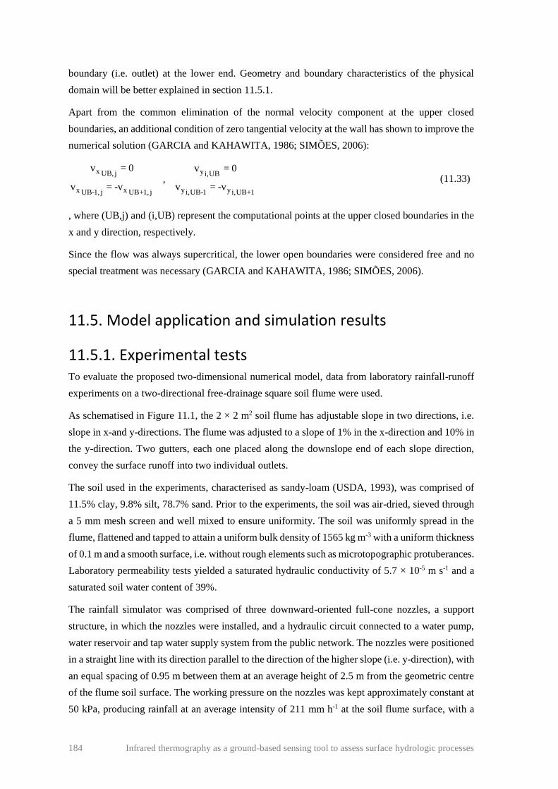
184 Infrared thermography as a ground-based sensing tool to assess surface hydrologic processes

boundary (i.e. outlet) at the lower end. Geometry and boundary characteristics of the physical

domain will be better explained in section 11.5.1.

Apart from the common elimination of the normal velocity component at the upper closed

boundaries, an additional condition of zero tangential velocity at the wall has shown to improve the

numerical solution (GARCIA and KAHAWITA, 1986; SIMÕES, 2006):

x yUB, j i,UB

x x y yUB-1, j UB+1, j i,UB-1 i,UB+1

v = 0 v = 0,

v = -v v = -v (11.33)

, where (UB,j) and (i,UB) represent the computational points at the upper closed boundaries in the

x and y direction, respectively.

Since the flow was always supercritical, the lower open boundaries were considered free and no

special treatment was necessary (GARCIA and KAHAWITA, 1986; SIMÕES, 2006).

11.5. Model application and simulation results

11.5.1. Experimental tests To evaluate the proposed two-dimensional numerical model, data from laboratory rainfall-runoff

experiments on a two-directional free-drainage square soil flume were used.

As schematised in Figure 11.1, the 2 × 2 m2 soil flume has adjustable slope in two directions, i.e.

slope in x-and y-directions. The flume was adjusted to a slope of 1% in the x-direction and 10% in

the y-direction. Two gutters, each one placed along the downslope end of each slope direction,

convey the surface runoff into two individual outlets.

The soil used in the experiments, characterised as sandy-loam (USDA, 1993), was comprised of

11.5% clay, 9.8% silt, 78.7% sand. Prior to the experiments, the soil was air-dried, sieved through

a 5 mm mesh screen and well mixed to ensure uniformity. The soil was uniformly spread in the

flume, flattened and tapped to attain a uniform bulk density of 1565 kg m-3 with a uniform thickness

of 0.1 m and a smooth surface, i.e. without rough elements such as microtopographic protuberances.

Laboratory permeability tests yielded a saturated hydraulic conductivity of 5.7 × 10-5 m s-1 and a

saturated soil water content of 39%.

The rainfall simulator was comprised of three downward-oriented full-cone nozzles, a support

structure, in which the nozzles were installed, and a hydraulic circuit connected to a water pump,

water reservoir and tap water supply system from the public network. The nozzles were positioned

in a straight line with its direction parallel to the direction of the higher slope (i.e. y-direction), with

an equal spacing of 0.95 m between them at an average height of 2.5 m from the geometric centre

of the flume soil surface. The working pressure on the nozzles was kept approximately constant at

50 kPa, producing rainfall at an average intensity of 211 mm h-1 at the soil flume surface, with a

Infrared thermography as a ground-based sensing tool to assess surface hydrologic processes 185

uniformity coefficient of 64.6%, calculated according to CHRISTIANSEN (1942). Spatial

distribution of the rainfall intensity at the soil surface is shown in Figure 11.2.

Figure 11.1. Experimental tests: a) Sketch of the laboratory set-up with the square soil flume and

rainfall simulator comprising the water reservoir and pump, hydraulic circuit and nozzles

(adapted from Deng et al., 2008); and b) Photograph of the 2 × 2 m2 soil flume with adjustable

slope in x-and y-directions (represented by the arrows), with indication of downslope gutters.

Figure 11.2. Rainfall intensity spatial distribution at the soil surface level. Major isohyets (black

lines) are in m s-1. Interval between minor isohyets (grey lines) is 0.5 × 10-5 m s-1. The arrows

represent the slope in x- and y-directions.

soil flume

water pump

and reservoir

nozzles

downslope gutters

soil surface

a) b)

hydraulic

circuit

y-d

irec

tio

n

x-direction

Rainfall intensity (m s-1)

186 Infrared thermography as a ground-based sensing tool to assess surface hydrologic processes

The experiments consisted on four rainfall simulations each lasting 5 min, with a 48 h interval of

no rain between them. The first rainfall was simulated on an initially dry soil condition with a low

soil water content of 0.1%. Initial soil moisture for the following events was the resulting from the

previous rainfall simulations and drying period. Before the start of a new event, the amount of

transported sediments in the previous event was replaced and the soil surface was levelled so that

microrelief (e.g. rills) formed during the previous event was removed, resulting in a new smooth

soil surface.

Samples of surface runoff of the x- and y-directions were collected separately at the two outlets

located at the downslope end of the soil flume, using metal containers. Sediments transported by

surface runoff were estimated by drying of samples in a low temperature oven.

11.5.2. Model parameterisation The following parameters were estimated using the data collected from the laboratory experiments:

i) Clear water density (ρ) and kinematic viscosity (υ), for water at a temperature of 20ºC, were fixed

in 998.2 kg m-3 and 1.003 × 10-6 m2 s-1, respectively, according to VENNARD and STREET (1975);

ii) Mean sediment particle diameter (ds) was estimated from the soil granulometric analysis and

was fixed to 4.0 × 10-4 m; iii) Soil porosity was estimated as equivalent to the saturated water

content and was fixed to 0.39; and iv) Sediment particles density (ρs) was estimated using the

measured soil bulk density of 1565 kg m-3 and estimated porosity of 0.39 and was fixed to 2566 kg

m-3.

The following parameters were estimated using the data from similar experimental work using the

same laboratory set-up (i.e. soil, soil flume, rainfall simulator) and similar numerical work using

similar numerical equations to express soil erosion (DENG et al., 2008): i) Manning’s roughness

coefficient (n) was fixed to 0.0265 s m-1/3; and ii) Interrill and rill erosion control parameters (η and

ξ) were fixed in 1.38 m-1 and 8.2 × 10-6 m1.2, respectively.

The dimensionless critical Shields parameter (θc) was estimated from PETIT (1994) and was fixed

in 0.047.

The parameters involved in the numerical simulation of infiltration (CN and cf) were obtained after

calibration till achievement of the best model performance. Such parameters are listed in Table

11.1.

Spatial discretization in both x- and y-directions (Δx and Δy) was fixed to 0.01 m.

Table 11.1. Infiltration parameters used in the proposed model, for each of the four rainfall-runoff

events.

Rainfall event

Infiltration parameter 1st 2nd 3rd 4th

CN (-) 95.0 99.0 99.5 99.5

cf (-) 0.200 0.050 0.050 0.025

Infrared thermography as a ground-based sensing tool to assess surface hydrologic processes 187

11.5.3. Model evaluation Different criteria were used to evaluate the performance of the numerical model. Firstly, the

accuracy of estimated runoff peak (Qp) and volume (V) and transported sediments peak (Qsp) and

total mass (Ms) and was quantified using the relative error (Er):

r

Obs - ModE = ×100

Obs (11.34)

, where Obs and Mod represent the observed and modelled data, respectively.

Secondly, the goodness of fit of the shape of the estimated runoff hydrographs and graphs of

transported sediments was quantified using the Coefficient of determination (r2) and the Nash-

Sutcliffe coefficient of efficiency (NS) according to NASH and SUTCLIFFE (1970):

( ) ( )( )

( ) ( )

2n

i i2 i=1

n n2 2

i i

i=1 i=1

Obs - Obs × Mod - Mod

r =

Obs - Obs × Mod - Mod

(11.35)

( )

( )

n2

i i

i 1n 2

i

i 1

Obs Mod

NS 1

Obs Obs

=

=

−

= −

−

(11.36)

, where Obsi and Modi represent the observed and modelled data at point i, respectively, Obs and

Mod represent the average observed and modelled data and n is the total number of data points.

11.5.4. Simulation results Graphs of experimentally observed (markers) and numerically modelled (solid curves) runoff (left)

and transported sediments (right) for the four simulated rainfall events, are shown in Figure 11.3.

Results of experimentally observed (Obs) and numerically modelled (Mod) runoff peak (Qp) and

runoff volume (V) and transported sediments peak (Qsp) and total mass (Ms), for the four rainfall-

runoff events, are shown in Tables 11.2 and 11.3; the Relative error (Er), the Coefficient of

determination (r2) and the Nash-Sutcliffe coefficient of efficiency (NS) comparing observed to

modelled results are also shown.

When compared to the higher slope of 10% in the y-direction, the lower slope of 1% in the x-

direction produced remarkably lower runoff and transported sediments (Figure 11.3). Overall, this

situation was more pronounced in the numerical model than in the experimental tests (see Er in

Tables 11.2 and 11.3).

188 Infrared thermography as a ground-based sensing tool to assess surface hydrologic processes

Figure 11.3. Graphs of observed (markers) and modelled (solid curves) runoff (left) and

transported sediments (right) fin the x- and y-directions and for each of the four rainfall-runoff

events: a) 1st rainfall event; b) 2nd rainfall event; c) 3rd rainfall event; and d) 4th rainfall event.

Infrared thermography as a ground-based sensing tool to assess surface hydrologic processes 189

The numerical model significantly underestimated x-direction runoff and transported sediments,

both in terms of peak and total amounts. In terms of numerical modelling goodness of fit, this

situation translated in a good performance in the y-direction as opposed to a poor performance in

the x-direction (see r2 and NS in Tables 11.2 and 11.3). For the x-direction, NS was always negative

for both runoff and transported sediments. For the y-direction, NS was always higher than 0.75

meaning a very good performance. Despite this results, r2 values were always higher than 0.75,

meaning a good correlation between observed and modelled data, even for the x-direction. Only

runoff results in the x-direction in the first rainfall event showed a different behaviour from the

other results. Here, x-direction runoff was overestimated and r2 value was close to 0.

Table 11.2. Observed (Obs) and modelled (Mod) results of runoff peak (Qp) and runoff volume

(V) for the four rainfall-runoff events. Relative error (Er), Coefficient of determination (r2) and

Nash-Sutcliffe coefficient of efficiency (NS) are shown.

Runoff

Rainfall

event Direction Data

Qp V r2 NS

ml s-1 Er (%) l Er (%)

1

x Obs 22.94

79.57 2.39

69.47 0.02 -1.16 Mod 4.69 0.73

y Obs 149.06

-2.38 24.18

-6.56 0.93 0.90 Mod 152.61 25.77

Total Obs 157.67

0.23 26.58

0.29 0.96 0.95 Mod 157.30 26.50

2

x Obs 5.34

-50.39 1.09

-80.33 0.51 -2.61 Mod 8.03 1.97

y Obs 228.73

4.03 55.70

-0.72 0.99 0.99 Mod 219.52 56.09

Total Obs 230.43

1.25 56.79

-2.25 0.99 0.98 Mod 227.55 58.06

3

x Obs 4.58

-84.05 1.25

-82.28 0.80 -12.99 Mod 8.43 2.28

y Obs 232.15

2.41 64.11

2.15 0.96 0.92 Mod 226.54 62.73

Total Obs 236.66

0.71 65.36

0.54 0.96 0.92 Mod 234.97 65.01

4

x Obs 5.96

-42.31 1.27

-81.39 0.83 -3.01 Mod 8.49 2.30

y Obs 237.82

4.15 63.68

0.51 0.99 0.98 Mod 227.95 63.35

Total Obs 241.80

2.22 64.95

-1.09 0.99 0.98 Mod 236.44 65.66

190 Infrared thermography as a ground-based sensing tool to assess surface hydrologic processes

Table 11.3. Observed (Obs) and modelled (Mod) results of transported sediment peak (Qsp) and

total mass (Ms) for the four rainfall-runoff events. Relative error (Er), Coefficient of

determination (r2) and Nash-Sutcliffe coefficient of efficiency (NS) are shown.

Transported sediments

Rainfall

event Direction Data

Qsp × 102 Ms r2 NS

g m2 s-1 Er (%) g Er (%)

1

x Obs 0.50

-13.70 2.31

-2.83 0.79 -0.79 Mod 0.57 2.38

y Obs 34.07

-10.89 188.97

-7.95 0.85 0.80 Mod 37.78 204.00

Total Obs 34.57

-10.93 191.28

-7.89 0.85 0.80 Mod 38.35 206.38

2

x Obs 4.96

70.03 17.26

24.28 0.82 -0.08 Mod 1.49 13.07

y Obs 74.28

7.24 634.54

-3.81 0.85 0.80 Mod 68.90 658.74

Total Obs 75.61

6.90 651.80

-3.07 0.85 0.79 Mod 70.39 671.81

3

x Obs 0.85

-88.47 6.86

-139.52 0.75 -8.97 Mod 1.61 16.44

y Obs 69.39

-4.46 690.12

-12.26 0.91 0.79 Mod 72.49 774.73

Total Obs 69.99

-5.87 696.33

-13.62 0.91 0.79 Mod 74.10 791.17

4

x Obs 1.17

-39.22 9.28

-80.77 0.87 -2.02 Mod 1.63 16.78

y Obs 74.05

1.11 688.33

-14.39 0.88 0.76 Mod 73.23 787.41

Total Obs 74.69

-0.22 697.61

-15.28 0.88 0.76 Mod 74.86 804.19

As expected, due to the initial dry soil condition, observed time to runoff was significantly higher

in the first rainfall event (60 s) when compared to the following events (20, 15 and 14 s). Also, the

hydrograph and sediment transport graph in the first event presented significantly less steep rising

limbs and lower peaks. The last three rainfall events presented similar results due to the similar

initial wet condition of the soil (i.e. 24h dry period between rainfall events). In numerical terms,

since infiltration parameters were calibrated according to each rainfall event, the initial soil

moisture condition did not had a visible impact in the performance model.

Since runoff and transported sediments in the x-direction were almost meaningful, the numerical

performance of the model in total terms (i.e. x- plus y-direction) was considered to be very good.

Overall, runoff was slightly better modelled than sediment transport. However, as stated before,

whereas the infiltration parameters were calibrated according to each rainfall event the sediment

transport parameters were fixed for all rainfall events.

Infrared thermography as a ground-based sensing tool to assess surface hydrologic processes 191

11.6. Conclusion

A two-dimensional mathematical model was developed for simulating soil erosion and sediment

transport resulting from rainfall induced overland flow. The model comprised: i) Two-dimensional

unsteady water flow equations on an infiltrating surface; ii) Combined Horton-SCS infiltration

scheme; and iii) Two-dimensional sediment transport equation with three distinct soil erosion

processes (interrill erosion, rill erosion and sediment deposition).

Overall, if the sum of the x- and y-direction results is considered, the numerically simulated graphs

of runoff and sediment transport were in very good agreement with corresponding experimental

measurements, demonstrating the laboratory proof-of-concept of the model. However, if x- and y-

directions results are analysed separately, the numerical model was only able to properly simulate

the runoff and sediment transport observed in the y-direction with the higher slope of 10%. A poor

agreement was observed for the remarkably lower values of runoff and sediment transport observed

in the x-direction with the lower slope of 1%. Overall, since the infiltration parameters were

calibrated, the initial moisture condition of the soil did not had impact on the performance of the

numerical model.

Although the agreement between the presented model and the experimental observations of runoff

and sediment transport were satisfactory, a performance evaluation of the spatial and temporal

evolution of flow velocity, flow depth, soil surface moisture conditions, soil surface microrelief

development (e.g. rills) and rainfall characteristics, should be performed. Future experimental tests

should contemplate such measurements, e.g. using new instrumental methodologies based on

infrared thermography such as the ones presented in ABRANTES et al. (2014, 2016, 2017, 2018a,

2019), DE LIMA and ABRANTES (2014a, 2014b), DE LIMA et al. (2014a, 2014b, 2014c, 2015a,

2015b) and MUJTABA and DE LIMA (2018).

“No research is ever quite complete. It is the glory of a good bit of work that it opens the way

for something still better, and this repeatedly leads to its own eclipse.”

- Mervin Gordon

"The outcome of any serious research can only be to make two questions grow where only one

grew before."

- Thorstein Veblen

Infrared thermography as a ground-based sensing tool to assess surface hydrologic processes 195

12. FINAL REMARKS

The first part of this chapter summarizes the overall conclusions reached during this doctoral study.

The second part attempts to give an answer to the main research question of this Thesis. The third

part presents some suggestions for future research.

12.1. Conclusions

The aim of this Thesis was to develop and investigate innovative techniques based on infrared

thermography that can be used as sensing tools to assess different hydrologic processes that occur

at the soil surface, namely in the study of surface runoff and water erosion. For that, seven specific

objectives were defined in Chapter 1. Those research objectives were achieved during this doctoral

study and the overall conclusions of this Thesis are drawn in the following paragraphs.

Objective 1. To develop, in laboratory, an innovative technique based on infrared thermography to

assess morphological characteristics of soil surface.

• The technique allows to identify the spatial variability of soil surface microrelief, rill

geometry and preferential flow paths at the soil surface;

• Visual thermal patterns distinguished in the infrared imaging are driven by differences in

hot water depth at the soil surface, i.e. hot water concentrates more in lower morphologic

features, therefore presenting different temperature than higher morphologic features;

• Thermal data can be converted into 3D models of the soil surface, using elevation point

measurements.

Objective 2. To develop, in laboratory, innovative techniques based on infrared thermography to

assess different hydraulic characteristics of soil surface.

• The technique allows to identify the spatial variability of soil surface permeability,

macroporosity and soil water repellency;

• Visual thermal patterns distinguished in the infrared imaging are driven by differences in

hot or cold water content in the soil and hot or cold water accumulation; i.e. hot or cold

water infiltrates more in more permeable and less water repellent areas and flows

preferentially to the macropores, therefore presenting different temperature than less

permeable areas, more water repellent areas and areas without macropores;

196 Infrared thermography as a ground-based sensing tool to assess surface hydrologic processes

• Thermal data can be converted into maps of soil surface permeability and soil water

repellency, using point measurements of soil hydraulic conductivity and surface tension,

respectively.

Objective 3. To investigate the applicability in real field conditions of an innovative technique

based on infrared thermography to assess the hydraulic behaviour of the soil surface due to

differences in soil water repellency.

• The applicability of the technique in real field conditions is comparable to the applicability

in controlled laboratory conditions, presenting very similar experimental set-up,

application methodology and measuring accuracy;

• The natural spatial variability of soil surface temperature in the field (i.e. before the

application of the technique), requires an adaptation of the data treatment procedure.

Objective 4. To identify the strengths and drawbacks of the techniques based on infrared

thermography developed in this doctoral study.

The following strengths of the techniques were identified:

• The techniques can be used in a very expedite way;

• The techniques are specifically useful to identify the spatial variability of morphologic

structures and visualise preferential flow paths at the soil surface in the presence of mulch

(i.e. organic residue covering the soil surface), where other techniques

(e.g. photogrammetry and laser techniques) may not be applied with success;

• The easy handling and low cost of the equipment (i.e. infrared camera, recipient with water

hotter or colder than the soil surface) compared with other techniques (e.g. laser scanners)

make them useful for measuring the spatial variation of soil surface characteristics;

• The fast application makes them interesting techniques to obtain spatially distributed data,

when compared to some time-consuming point measurement techniques (e.g. pin or relief

meters, constant head permeameters, MED test);

• The techniques are independent of illumination condition, which is known to severely

affect optical and laser measurement techniques; furthermore, the techniques based on

infrared thermography can be used during night-time without artificial lighting.

The following drawbacks of the techniques were identified:

• Overall, the precision of the techniques in measure the spatial variation of soil surface

characteristics is low compared with other more accurate measurement techniques

(e.g. photogrammetry and laser techniques);

• The precision of some techniques relies on point measurements of surface morphology and

hydraulic characteristics (e.g. with a pin meter, double ring infiltrometer, MED test);

Infrared thermography as a ground-based sensing tool to assess surface hydrologic processes 197

• Due to heat propagation in the soil, sharp variations of soil surface characteristics (e.g. rill

and macropores geometry) tend to be interpreted as being smoother;

• The assessment of a determined soil surface morphologic or hydraulic characteristic can

be affected by the spatial variability of other soil surface morphologic and hydraulic

characteristics; e.g. high variable soil surface morphology (e.g. rills, ponds, mounds) or the

presence of macropores at the soil surface can affect the assessment of soil surface

permeability or soil water repellency;

• The techniques themselves can affect the soil surface morphology and hydraulic

characteristics, so a second test in easy erodible soils may obtain a slightly different result.

Objective 5. To investigate the use of thermal tracers and infrared video cameras to estimate the

velocity of shallow flows.

• The visualization of the movement of a thermal tracer within flowing water, using an infrared

camera, can be used to measure the surface velocity of distributed overland flows and

concentrated rill flows, as well as to identify preferential flow paths at the surface of the

water;

• Overall, thermal tracer velocities are slightly higher than velocities measured using other

traditional and well-established tracer techniques, such as dye and salt tracers; however,

differences are not significant;

• The correction factors used to estimate the mean flow velocity from the tracers’

measurements greatly vary with the hydraulic characteristics of the flow (e.g. velocity, depth,

Reynolds number, Froude number) and the characteristics of the bottom surface

(e.g. roughness, slope);

The main advantage of using thermal tracers are:

• Higher visibility compared with the dye tracers, which leads to the estimation of flow

velocity using smaller volume of tracer, and, therefore, smaller disturbances in the actual

flow velocity;

• Easier image processing than dye tracers that usually require more sophisticated and

specific light conditions that may not be always available, especially in field tests;

• The visualization of the movement of the tracer within the flow, which cannot be done with

salt tracing;

• The possibility of measuring the flow velocity without the need of introducing any

instrument (e.g. sensor) in the flow, causing less disturbances in the actual flow velocity;

• Non-necessity of a minimum water depth, which usually is needed to accurately measure

flow velocity with some instruments (e.g. sensors);

198 Infrared thermography as a ground-based sensing tool to assess surface hydrologic processes

• Thermal tracers are more environmentally friendly than dye and salt tracers; they are

cleaner and more ecological, do not leave any residue in the water or the soil and cause

very little temporal and spatial disturbance on the environment.

The main disadvantages of using thermal tracers are:

• Higher price of an infrared video camera compared with a regular optical video camera or

an electrolyte sensor, despite recent falls in the cost of infrared equipment;

• The necessity of water hotter or colder than the flowing water may be an obstacle in remote

field places;

• Thermal tracers are less conservative than salt tracers;

• Measuring flow velocity using the dye tracer can be faster and more intuitive than the

thermal tracer, since the movement of the tracer can be simply observed by the operator

without using any recording equipment; however, at the cost of a worst accuracy;

Objective 6. To develop a numerical approach to combine with thermal tracers to estimate basic

hydraulic characteristics of shallow flows.

• The developed numerical approach by fitting an analytical solution of an advection–

dispersion transport equation to temperature data from thermal tracers can be used to estimate

the velocity and the dispersion coefficient (hydrodynamic or thermal) of shallow flows;

• Results from the numerical methodology predicted the mean flow velocity better than other

more traditional and well-established methodologies, such as measuring the leading edge and

centroid of the tracer.

Objective 7. To develop a two-dimensional (2D) rainfall induced water erosion numerical model.

• The mathematical model comprises a rainfall-runoff module using the 2D unsteady

physically based Saint-Venant equations, a rainfall-infiltration module using a combined

Horton-SCS empirical scheme and a water erosion and sediment transport module using a

2D transport rate-based advection equation and a detachment-transport-deposition

approach, distinguishing between interrill erosion, rill erosion and sediment deposition;

• The governing equations are solved using an explicit finite-differences method based on

the MacCormack operator-splitting scheme;

• The parameterization and calibration procedure of the model can be difficult due to the

large amount of simulation parameters;

• Overall, the numerically simulated graphs of runoff and sediment transport are in very good

agreement with corresponding experimental measurements; even so, lower volumes of

runoff and sediment transport are not so well simulated as higher volumes.

Infrared thermography as a ground-based sensing tool to assess surface hydrologic processes 199

12.2. Answer to research question

In Chapter 1, the following research question was presented to be discussed and analysed in this

Thesis: Can information collected at the soil surface level with techniques based on infrared

thermography be useful to model and better understand surface hydrologic processes?

The research presented in this doctoral study revealed that infrared thermography can be used as a

ground-based sensing tool for acquisition of information on soil surface characteristics and flow

hydraulics. These techniques have shown great potential to: i) Estimate the spatial variability of

soil surface morphology where other techniques cannot be applied (e.g. presence of organic

residues concealing the soil surface); ii) Estimate the spatial variability of soil surface hydraulic

characteristics in a faster and expedite way, instead of multiple time-consuming point

measurements that need to be grouped or scaled to bring out spatial coherence; and iii) Estimate

the surface flow velocity in the occurrence of very shallow flows where many measurement

equipment cannot be used.

One big advantage of these techniques is the possibility of qualitative real time monitoring of the

spatial dynamics of some key processes in surface hydrology, using a fast and expedite

methodology with a simple set-up and only one equipment, i.e. one infrared video camera. Usually,

gathering such amount of data would normally require different types of equipment, more complex

setups, time-consuming methodologies and specialized personal. However, in quantitative terms,

the precision of some of these techniques relies on measurements with other more common

techniques. As usual, such novel sensing tools will need thorough assessment to be routinely

adopted in field monitoring practices. Their development will require extensive calibration,

validation and collaboration from the scientific community.

Observations from these techniques can be used to complement observations from other techniques.

Also, nowadays, the technological advances provide a great variety of equipment and technologies

that can be combined, taking advantage each other’s potentials, e.g. dual cameras with optical and

infrared sensors to combine optical and infrared observations, infrared cameras couple with

unmanned aerial vehicles to combine observations at different scales. Main attention should be

drawn to the ability to complement these new observations with other observations from other

techniques with different temporal and spatial resolutions, different precisions and different

physical meanings.

No doubt, the information collected with these innovative techniques based on infrared

thermography can be useful to calibrate and validate numerical models of surface hydrology, such

as surface runoff and water erosion, as well as to better understand the underlying processes.

200 Infrared thermography as a ground-based sensing tool to assess surface hydrologic processes

12.3. Future work

Further research could include:

• Extensive field testing at different spatial and temporal scales and different soil surface and

hydraulic conditions to calibrate and validate these innovative techniques as suitable

monitoring techniques for surface hydrology;

• Investigation on the use of infrared cameras to asses other hydrologic processes at the soil

surface, such as ponding;

• Investigation on the use of dual cameras with infrared and optical sensors to assess surface

hydrologic processes combining both observations;

• Coupling of infrared cameras with unmanned aerial vehicles to gather data at different

spatial scales;

• Development of a numerical algorithm to analyse thermal imaging (or thermal and optical

imaging) and automatically identify the different morphologic and hydraulic characteristics

of the soil surface;

• Installation of equipment (e.g. infrared cameras, automatic thermal tracer devices) in

natural systems or at existing observation stations to continuous automatic monitoring of

surface hydrologic processes;

• Carry out of laboratory and field experiments focusing on water erosion, applying the

developed innovative techniques based on infrared thermography, in order to validate the

developed numerical model.

“The common facts of today are the products of yesterday’s research.”

- Duncan MacDonald

Infrared thermography as a ground-based sensing tool to assess surface hydrologic processes 203

13. REFERENCES

ABRAHAMS, A.D. and ATKINSON, J.F. (1993). Relation between grain velocity and sediment

concentration in overland flow. Water Resources Research, 29(9), 3021-3028.

DOI:10.1029/93WR00771.

ABRAHAMS, A.D., PARSONS, A.J. and LUK, S.H. (1986). Field measurement of the velocity of

overland flow using dye tracing. Earth Surface Processes and Landforms, 11(6), 653-657.

DOI:10.1002/esp.3290110608.

ABRANTES, J.R.C.B. and DE LIMA, J.L.M.P. (2014). Termografia para determinação da

microtopografia da superfície do solo em diferentes condições de cobertura morta. Revista

Brasileira de Ciências Agrárias, 9(3), 445-453. DOI:10.5039/agraria.v9i3a3602.

ABRANTES, J.R.C.B., DE LIMA, J.L.M.P. and MONTENEGRO, A.A.A. (2015). Desempenho

da modelagem cinemática do escoamento superficial para chuvas intermitentes em solos com

cobertura morta. Revista Brasileira de Engenharia Agrícola e Ambiental, 19(2), 166-172.

DOI:10.1590/1807-1929/agriambi.v19n2p166-172.

ABRANTES, J.R.C.B., DE LIMA, J.L.M.P., PRATS, S.A. and KEIZER, J.J. (2017). Assessing

soil water repellency spatial variability using a thermographic technique: an exploratory study

using a small-scale laboratory soil flume. Geoderma, 287, 98-104.

DOI:10.1016/j.geoderma.2016.08.014.

ABRANTES, J.R.C.B., DE LIMA, J.L.M.P., PRATS, S.A. and KEIZER, J.J. (2016). Field

assessment of soil water repellency using infrared thermography. Forum Geographic, 15(2), 12-

18. DOI:10.5775/fg.2016.019.s.

ABRANTES, J.R.C.B., MORUZZI, R.B., DE LIMA, J.L.M.P., SILVEIRA, A. and

MONTENEGRO, A.A.A. (2019). Combining a thermal tracer with a transport model to estimate

shallow flow velocities. Physics and Chemistry of the Earth, 109, 59-69.

DOI:10.1016/j.pce.2018.12.005.

ABRANTES, J.R.C.B., MORUZZI, R.B., SILVEIRA, A., DE LIMA, J.L.M.P. (2018a).

Comparison of thermal, salt and dye tracing to estimate shallow flow velocities: novel triple

tracer approach. Journal of Hydrology, 557, 362-377. DOI:10.1016/j.jhydrol.2017.12.048.

ABRANTES, J.R.C.B., PRATS, S.A., KEIZER, J.J., and DE LIMA, J.L.M.P. (2018b).

Effectiveness of the application of rice straw mulching strips in reducing runoff and soil loss:

Laboratory soil flume experiments under simulated rainfall. Soil & Tillage Research, 180, 238-

249. DOI:10.1016/j.still.2018.03.015.

ALI, M., SEEGER, M., STERK, G. and MOORE, D. (2013). A unit stream power based sediment

transport function for overland flow. CATENA, 101, 197-204.

DOI:10.1016/j.catena.2012.09.006.

ALLAIRE, S.E., ROULIER, S. and CESSNA, A.J. (2009). Quantifying preferential flow in soils:

a review of different techniques. Journal of Hydrology, 378(1-2), 179-204.

DOI:10.1016/j.jhydrol.2009.08.013.

ALLMARAS, R.R., BURWELL, R.E., LARSON, W.E. and HOLT, R.F. (1966). Total porosity

and random roughness of the interrow zone as influenced by tillage. Conservation Research

Report No. 7. Washington, DC, USA: USDA. 22 pp.

204 Infrared thermography as a ground-based sensing tool to assess surface hydrologic processes

APPLES, W.M. (2013). Water redistribution at the soil surface: ponding and surface runoff in flat

areas. PhD Thesis, Wageningen University, Wageningen, The Netherlands. 164 pp.

BAARTMAN, J.E.M., JETTEN, V.G., RITSEMA, C.J. and DE VENTE, J. (2011). Exploring

effects of rainfall intensity and duration on soil erosion at the catchment scale using open

LISEM: Prado catchment, SE Spain. Hydrological Processes, 26 (7), 1034-1049.

DOI:10.1002/hyp.8196.

BACHMANN, J., ELLIES, A. and HARTGE, K.H. (2000). Development and application of a new

sessile drop contact angle method to assess soil water repellency. Journal of Hydrology, 231-

232, 66-75. DOI:10.1016/S0022-1694(00)00184-0.

BADÍA-VILLAS, D., GONZÁLEZ-PÉREZ, J.A., AZNAR, J.M., ARJONA-GRACIA, B. and

MARTÍ-DALMAU, C. (2014). Changes in water repellency, aggregation and organic matter of

a mollic horizon burned in laboratory: soil depth affected by fire. Geoderma, 213, 400-407.

DOI:10.1016/j.geoderma.2013.08.038.

BAGAVATHIAPPAN, S., SARAVANAN, T., PHILIP, J. and JAYAKUMAR, T. (2013). Infrared

thermography for condition monitoring - a review. Infrared Physics & Technology, 60, 35-55.

DOI:10.1016/j.infrared.2013.03.006.

BAKER, E.A., LAUTZ, L.K., MCKENZIE, J.M. and AUBRY-WAKE, C. (2019). Improving the

accuracy of time-lapse thermal infrared imaging for hydrologic applications. Journal of

Hydrology, 571, 60-70. DOI:10.1016/j.jhydrol.2019.01.053.

BAN, Y., LEI, T., LIU, Z. and CHEN, C. (2016). Comparison of rill flow velocity over frozen and

thawed slopes with electrolyte tracer method. Journal of Hydrology, 534, 630-637.

DOI:10.1016/j.jhydrol.2016.01.028.

BATISTA, P.V.G., DAVIES, J., SILVA, M.L.N. and QUINTON, J.N. (2019). On the evaluation

of soil erosion models: are we doing enough? Earth-Science Reviews, 197, 102898.

DOI:10.1016/j.earscirev.2019.102898.

BAUER, S.W. (2010). A modified Horton equation for infiltration during intermitente rainfall.

Hydrological Sciences Bulletin, 19(2), 219-225. DOI:10.1080/02626667409493900.

BENTLEY, A. (1904). Studies of raindrops and raindrop phenomena. Monthly Weather Review,

32, 450-456. DOI:10.1175/1520-0493(1904)32<450:SORARP>2.0.CO;2.

BERGER, C., SCHULZE, M., RIEKE-ZAPP, D. and SCHULUNEGGER, F. (2010). Rill

development and soil erosion: a laboratory study of slope and rainfall intensity. Earth Surface

Processes and Landforms, 35 (12), 1456–1467. DOI:10.1002/esp.1989.

BEVEN, K. (2004). Robert E. Horton’s perceptual model of infiltration processes. Hydrological

Processes, 18 (17), 3447-3460.

BEVEN, K.J. and GERMANN, P.F. (1982). Macropores and water flow in soils. Water Resources

Research, 18 (5), 1311-1325. DOI:10.1029/WR018i005p01311.

BEVEN, K.J. and GERMANN, P.F. (2013). Macropores and water flow in soils revisited. Water

Resources Research, 49 (6), 3071-3092. DOI:10.1002/wrcr.20156.

BEVEN, K.J., KIRKBY, M.J., SCHOFIELD, N. and TAGG, A.F. (1984). Testing a physically-

based flood forecasting model (TOPMODEL) for three U.K. catchments. Journal of Hydrology,

69(1-4), 119-143. DOI:10.1016/0022-1694(84)90159-8.

BEVEN, K.J., ZHANG, D. and MERMOUD, A. (2006). On the value of local measurements on

prediction of pesticide transport at the field scale. Vadoze Zone Journal, 5(1), 222-233.

DOI:10.2136/vzj2005.0016.

BJERKLIE, D.M., (2007). Estimating the bankfull velocity and discharge for rivers using remotely

sensed river morphology information. Journal of Hydrology, 341(3-4), 144-155.

DOI:10.1016/j.jhydrol.2007.04.011.

Infrared thermography as a ground-based sensing tool to assess surface hydrologic processes 205

BJERKLIE, D.M., DINGMAN, S.L., VOROSMARTY, C.J., BOLSTER, C.H. and

CONGALTON, R.G. (2003). Evaluating the potential for measuring river discharge from space.

Journal of Hydrology, 278(1-4), 13-78. DOI:10.1016/S0022-1694(03)00129-X.

BLANCHOUD, H., MOREAU-GUIGON, E., FARRUGIA, F., CHEVREUIL, M. and

MOUCHEL, J. M. (2007). Contribution by urban and agricultural pesticide uses to water

contamination at the scale of the Marne watershed. Science of the Total Environment, 375(1-3),

168-179. DOI:10.1016/j.scitotenv.2006.12.009.

BLÖSCHL, G. et al. (2019). Twenty-three Unsolved Problems in Hydrology (UPH): a community

perspective. Hydrological Sciences Journal, 64(10), 1141-1158,

DOI:10.1080/02626667.2019.1620507

BOARDMAN, J., SHEPHEARD, M.L., WALKER, E. and FOSTER, I.D.L. (2009). Soil erosion

and risk-assessment for on- and off-farm impacts: A test case using the Midhurst area, West

Sussex, UK. Journal of Environmental Management, 90(8), 2578-2588.

DOI:10.1016/j.jenvman.2009.01.018.

BOBBA, A.G., BUKATA, R.P. and JEROME, J.H. (1992). Digitally processed satellite data as a

tool in detecting potential groundwater flow systems. Journal of Hydrology, 31(1-4), 25-62.

DOI:10.1016/0022-1694(92)90212-E.

BOCHET, E., POESEN, J. and RUBIO, J.L. (2006). Runoff and soil loss under individual plants

of a semi-arid Mediterranean shrubland: influence of plant morphology and rainfall intensity.

Earth Surface Processes and Landforms, 31(5), 536-549. DOI:10.1002/esp.1351.

BONAR, S.A. and PETRE, S.J. (2015). Ground-based thermal imaging of stream surface

temperatures: technique and evaluation. North American Journal of Fisheries Management,

35(6), 1209-1218. DOI:10.1080/02755947.2015.1091410.

BONNER, R., AYLWARD, A., HARLEY, C., KAPPELMEYER, U. and SHERIDAN, C.M.

(2017). Heat as a hydraulic tracer for horizontal subsurface flow constructed wetlands. Journal

of Water Process Engineering, 16, 183-192. DOI:10.1016/j.jwpe.2017.01.007.

BRADLEY, S.G. and STOW, C.D. (1974). The measurement of charge and size of raindrops: part

I. The disdrometer. Journal of Applied Meteorology, 13(1), 114-130. DOI:10.1175/1520-

0450(1974)013<0114:TMOCAS>2.0.CO;2.

BRAUD, I., DE CONDAPPA, D., SORA, J.M., HAVERKAMP, R., ANGULO-JARAMILLO, R.,

GALLE, S. and VAUCLIN, M. (2005). Use of scaled forms of the infiltration equation for the

estimation of unsaturated soil hydraulics properties (the Beerkan method). European Journal of

Soil Science, 56 (3), 361-374. DOI:10.1111/j.1365-2389.2004.00660.x.

BUTZEN, V., SEEGER, M., WIRTZ, S., HUEMANN, M., MUELLER, C., CASPER, M. and

RIES, J.B. (2014). Quantification of Hortonian overland flow generation and soil erosion in a

Central European low mountain range using rainfall experiments. CATENA, 113, 202-212.

DOI:10.1016/j.catena.2013.07.008.

CALKINS, D. and DUNNE, T. (1970). A salt tracing method for measuring channel velocities in

small mountain streams. Journal of Hydrology, 11(4), 379-392. DOI:10.1016/0022-

1694(70)90003-X.

CANTÓN, Y., SOLÉ-BENET, A., DE VENTE, J., BOIX-FAYOS, C., CALVO-CASES, A.,

ASENSIO, C. and PUIGDEFÁBREGAS, J. (2011). A review of runoff generation and soil

erosion across scales in semiarid south-eastern Spain. Journal of Arid Environments, 75(12),

1254-1261. DOI:10.1016/j.jaridenv.2011.03.004.

CAO, Z., PENDER, G., WALLIS, S. and CARLING, P. (2002). Computational dam-break

hydraulics over erodible sediment bed. Journal of Hydraulic Engineering, 128(5), 460-72.

DOI:10.1061/(ASCE)0733-9429(2004)130:7(689).

206 Infrared thermography as a ground-based sensing tool to assess surface hydrologic processes

CARDENAS, M.B., HARVEY, J.W., PACKMAN, A.I. and SCOTT, D.T. (2008). Ground-based

thermography of fluvial systems at low and high discharge reveals potential complex thermal

heterogeneity driven by flow variation and bioroughness. Hydrological Processes, 22(7), 980-

986. DOI:10.1002/hyp.6932.

CARRILLO, M.L.K., LETEY, J. and YATES, S.R. (1999). Measurement of initial soil-water

contact angle of water repellent soils. Soil Science Society of America Journal, 63(3), 433-436.

DOI:10.2136/sssaj1999.03615995006300030002x.

CERDÀ, A. (1996). Seasonal variability of infiltration rates under contrasting slope conditions in

southeast Spain. Geoderma, 69 (3-4), 217-232. DOI:10.1016/0016-7061(95)00062-3.

CERDÀ, A. (2010). Seasonal and spatial variations in infiltration rates in badland surfaces under

Mediterranean climatic conditions. Water Resources Research, 35(1), 319-328.

DOI:10.1029/98WR01659.

CERDÀ, A., IBÁÑEZ, S. and CALVO, A. (1997). Design and operation of a small and portable

rainfall simulator for rugged terrain. Soil Technology, 11(2), 163-170. DOI:10.1016/S0933-

3630(96)00135-3.

CHAU, H.W., BISWAS, A., VUJANOVIC, V. and SI, B.C. (2014).Relationship between the

severity, persistence of soil water repellency and the critical soil water content in water repellent

soils. Geoderma, 221-222, 113-120. DOI:10.1016/j.geoderma.2013.12.025.

CHEN, C., BAN, Y., WANG, X. and LEI, T. (2017). Measuring flow velocity on frozen and non-

frozen slopes of black soil through leading edge method. International Soil and Water

Conservation Research, 5(3), 180-189. DOI:10.1016/j.iswcr.2017.02.004.

CHEN, X., SONG, J., CHENG, C., WANG, D. and LACKEY, S.O. (2009). A new method for

mapping variability in vertical seepage flux in streambeds. Hydrogeology Journal, 17(3), 519-

525. DOI:10.1007/s10040-008-0384-0

CHENG, N.S. (1997). Simplified settling velocity formula for sediment particle. Journal of

Hydraulic Engineering, 123(2), 149-152. DOI:10.1061/(ASCE)0733-9429(1997)123:2(149).

CHRISTIANSEN, J.E. (1942). Irrigation by Sprinkling. California Agricultural Experiment

Station Bulletin 670. Berkeley, CA, USA: University of California. 124 pp.

CLARKE, T. R. (1997). An empirical approach for detecting crop water stress using multispectral

airborne sensors. HortTechnology, 7(1), 9-16. DOI:10.21273/HORTTECH.7.1.9.

COCHRANE, T.A. and FLANAGAN, D.C. (1996). Detachment in a simulated rill. Transactions

of the American Society of Agricultural Engineers 40 (1), 111-119. DOI:10.13031/2013.21255.

COMINA, C., LASAGNA, M., DE LUCA, D.A. and SAMBUELLI, L. (2014). Geophysical

methods to support correct water sampling locations for salt dilution gauging. Hydrology and

Earth System Science, 18(8), 3195-3203. DOI:10.5194/hess-18-3195-2014.

COMITI, F., MAO, L., WILCOX, A., WOHL, E.E. and LENZI, M.A. (2007). Field-derived

relationships for flow velocity and resistance in high-gradient streams. Journal of Hydrology,

340(1-2), 48-62. DOI:10.1016/j.jhydrol.2007.03.021.

COOK, H.F., VALDES, G.S.B. and LEE, H.C. (2006). Mulch effects on rainfall interception, soil

physical characteristics and temperature under Zea mays L. Soil & Tillage Research, 91(1-2),

227-235. DOI:10.1016/j.still.2005.12.007.

COSENTINO, D., HALLETT, P.D., MICHEL, J.C. and CHENU, C. (2010). Do different methods

for measuring the hydrophobicity of soil aggregates give the same trends in soil amended with

residue? Geoderma, 159(1-2), 221-227. DOI:10.1016/j.geoderma.2010.07.015.

COZ, J.L., HAUET, A., PIEEFEU, G., DRAMAIS, G. and CAMENEN, B. (2010). Performance

of image-based velocimetry LSPIV applied to flash-flood discharge measurements in

Infrared thermography as a ground-based sensing tool to assess surface hydrologic processes 207

Mediterranean rivers. Journal of Hydrology, 394(1-2), 42-52.

DOI:10.1016/j.jhydrol.2010.05.049.

CUOMO, S., DELLA SALA, M. and PIERRI, M. (2016). Experimental evidences and numerical

modelling of runoff and soil erosion in flume tests. CATENA, 147, 61-70.

DOI:10.1016/j.catena.2016.06.044.

DANIELESCU, S., MACQUARRIE, K.T.B. and FAUX, R.N. (2009). The integration of thermal

infrared imaging, discharge measurements and numerical simulation to quantify the relative

contributions of freshwater inflows to small estuaries in Atlantic Canada. Hydrological

Processes, 23(20), 2847-2859. DOI:10.1002/hyp.7383.

DARBOUX, F. and HUANG, C. (2003). An instantaneous-profile laser scanner to measure soil

surface microtopography. Soil Science Society of America Journal, 67(1), 92-99.

DOI:10.2136/sssaj2003.9200.

DARBOUX, F., DAVY, PH., GASCUEL-ODOUX, C. and HUANG, C. (2001). Evolution of soil

surface roughness and flowpath connectivity in overland flow experiments. CATENA, 46(2-3),

124-139. DOI:10.1016/S0341-8162(01)00162-X.

DAY, T.J. (1977). Observed mixing lengths in mountain streams. Journal of Hydrology, 35(1-2),

125-136. DOI:10.1016/0022-1694(77)90081-6.

DE LIMA, C.A., DE LIMA, J.L.M.P., MONTENEGRO, A.A.A., ABRANTES, J.R.C.B.,

MUJTABA, B. and SILVEIRA, A. (2018). Comparative evaluation of factors influencing seed

displacement over the soil of nonconventional perennial crops: moringa (Moringa oleifera

Lam.) and neem (Azadirachta indica A. Juss.). Soil Science, 182(8), 267-277.

DOI:10.1097/SS.0000000000000219.

DE LIMA, J.L.M.P. and ABRANTES, J.R.C.B. (2014a). Can infrared thermography be used to

estimate soil surface microrelief and rill morphology? Catena, 113, 314-322.

DOI:10.1016/j.catena.2013.08.011.

DE LIMA, J.L.M.P. and ABRANTES, J.R.C.B. (2014b). Using a thermal tracer to estimate

overland and rill flow velocities. Earth Surface Processes and Landforms, 39(10), 1293-1300.

DOI:10.1002/esp.3523.

DE LIMA, J.L.M.P. and SINGH, V.P. (2002). The influence of the pattern of moving rainstorms

on overland flow. Advances in Water Resources, 25(7), 817-828. DOI:10.1016/S0309-

1708(02)00067-2.

DE LIMA, J.L.M.P., ABRANTES, J.R.C.B., SILVA JR., V.P., DE LIMA, M.I.P. and

MONTENEGRO, A.A.A. (2014a). Mapping soil surface macropores using infrared

thermography: exploratory laboratory study. Scientific World Journal, 2014, 845460.

DOI:10.1155/2014/845460.

DE LIMA, J.L.M.P., ABRANTES, J.R.C.B., SILVA, JR., V.P. and MONTENEGRO, A.A.A.

(2014b). Prediction of skin surface soil permeability by infrared thermography: a soil flume

experiment. Quantitative InfraRed Thermography Journal, 11(2), 161-169.

DOI:10.1080/17686733.2014.945325.

DE LIMA, J.L.M.P., CARVALHO, S.C.P. and DE LIMA, M.I.P. (2013a). Rainfall simulator

experiments on the importance of when rainfall burst occurs during storm events on runoff and

soil loss. Zeitschrift für Geomorphologie, 57(1), 91-109. DOI:10.1127/0372-8854/2012/S-

00096.

DE LIMA, J.L.M.P., DE LIMA, M.I.P. and SINGH, V.P. (2005). The importance of the direction,

speed, intensity and length of moving storms on water erosion. In A. FAZ CANO, R. ORTIZ

SILLA and A.R. MERMUT (Eds.), Advances in Geoecology 36 - Sustainable Use and

Management of Soils: Arid and Semiarid Regions. Reiskirchen, Germany: Catena Verlag. pp.

163-176.

208 Infrared thermography as a ground-based sensing tool to assess surface hydrologic processes

DE LIMA, J.L.M.P., DINIS, P.A., SOUZA, C.S., DE LIMA, M.I.P., CUNHA, P.P., AZEVEDO,

J.M., SINGH, V.P. and ABREU, J.M. (2011). Patterns of grain-size temporal variation of

sediment transported by overland flow associated with moving storms: interpreting soil flume

experiments. Natural Hazards and Earth System Science, 11, 2605-2615. DOI:10.5194/nhess-

11-2605-2011.

DE LIMA, J.L.M.P., SILVA JR., V.P., ABRANTES, J.R.C.B., MONTENEGRO, A.A.A. and DE

LIMA, M.I.P. (2014c). In situ observation of soil macropores using infrared thermography. Die

Bodenkultur: Journal of Land Management, Food and Environment, 65(3-4), 57-62. Retrieved

from https://boku.ac.at/en/fos/themen/die-bodenkultur/inhalte/band-65-2014/band-65-heft-3-

4/de-lima-silva.

DE LIMA, J.L.M.P., SILVA, JR., V.P., DE LIMA, M.I.P., ABRANTES, J.R.C.B. and

MONTENEGRO, A.A.A. (2015a). Revisiting simple methods to estimate drop size

distributions: a novel approach based on infrared thermography. Journal of Hydrology

Hydromechanics, 63(3), 220-227. DOI:10.1515/johh-2015-0025.

DE LIMA, J.L.M.P., SINGH, V.P. and DE LIMA, M.I.P. (2003). The influence of storm movement

on water erosion: Storm direction and velocity effects. CATENA, 52(1), 39-56.

DOI:10.1016/S0341-8162(02)00149-2.

DE LIMA, J.L.M.P., SOUZA, C.S. and SINGH, V.P. (2008). Granulometric characterization of

sediments transported by surface runoff generated by moving storms. Nonlinear Processes in

Geophysics, 15, 999-1011. DOI:10.5194/npg-15-999-2008.

DE LIMA, J.L.M.P., TAVARES, P., SINGH, V.P. and DE LIMA, M.I.P. (2009). Investigating the

nonlinear response of soil loss to storm direction using a circular soil flume. Geoderma, 152(1-

2), 9-15. DOI:10.1016/j.geoderma.2009.05.004.

DE LIMA, M.I.P. and GRASMAN, J. (1999). Multifractal analysis of 15-min and daily rainfall

from a semi-arid region in Portugal. Journal of Hydrology, 220(1-2), 1-11. DOI:10.1016/S0022-

1694(99)00053-0.

DE LIMA, M.I.P., ESPÍRITO SANTO, F., RAMOS, A.M. and DE LIMA, J.L.M.P. (2013b).

Recent changes in daily precipitation and surface air temperature extremes in mainland Portugal,

in the period 1941-2007. Atmospheric Research, 127, 195-209.

DOI:10.1016/j.atmosres.2012.10.001.

DE LIMA, M.I.P., SCHERTZER, D., LOVEJOY, S. and DE LIMA, J.L.M.P. (2002). Multifractals

and the study of extreme precipitation events: a case study from semi-arid and humid regions in

Portugal. In V.P. SINGH, M. AL-RASHID and M.M. SHERIF (Eds.), Surface Water

Hydrology. Rotterdam, The Netherlands: A.A. Balkema Publishers. pp. 195-211.

DE LIMA, R.L.P (2013). Development of a method using infrared thermography for shallow flow

visualization and quantitative estimation of velocity. MSc Thesis, University of Coimbra,

Coimbra, Portugal. 77 pp.

DE LIMA, R.L.P., ABRANTES, J.R.C.B., DE LIMA, J.L.M.P. and DE LIMA, M.I.P. (2015b).

Using thermal tracers to estimate flow velocities of shallow flows: laboratory and field

experiments. Journal of Hydrology Hydromechanics, 63(3), 255-262. DOI:10.1515/johh-2015-

0028.

DE MARSILY, G. (1986). Quantitative Hydrogeology: Groundwater Hydrology for Engineers.

San Diego, California, USA: Academic Press. 440 pp.

DE VENTE, J., POESEN, J., VERSTRAETEN, G., GOVERS, G., VANMAERCKE, M.,

ROMPAEY, A.V., ARABKHEDRI, M. and BOIX-FAYOS, C. (2013). Predicting soil erosion

and sediment yield at regional scales: where do we stand? Earth-Science Reviews, 127, 16-29.

DOI:10.1016/j.earscirev.2013.08.014.

Infrared thermography as a ground-based sensing tool to assess surface hydrologic processes 209

DEBANO, L.F. (2000a). The role of fire and soil heating on water repellency in wildland

environments: a review. Journal of Hydrology, 231-232, 195-206. DOI:10.1016/S0022-

1694(00)00194-3.

DEBANO, L.F. (2000b). SWR in soils: a historical overview. Journal of Hydrology, 231-232, 4-

32. DOI:10.1016/S0022-1694(00)00180-3.

DEHVARI, A. and HECK, R.J. (2007). Comparison of object-based and pixel based infrared

airborne image classification methods using DEM thematic layer. Journal of Geography and

Regional Planning, 2(4), 86-96. DOI:10.5897/JGRP2009.5B0C0A51198.

DEKKER, L.W. and RITSEMA, C.J. (1994). How water moves in a water-repellent sandy soil: 1.

Potential and actual water-repellency. Water Resources Research, 30(9), 2507-2517.

DOI:10.1029/94WR00749.

DEKKER, L.W., RITSEMA, C.J., OOSTINDIE, K., MOORE, D. and WESSELING, J.G. (2009).

Methods for determining soil water repellency on field-moist samples. Water Resources

Research 45(4), W00D33. DOI:10.1029/2008WR007070.

DENG Z.Q. DE LIMA J.L.M.P. and SINGH V.P. (2005). Transport rate-based model for overland

flow and solute transport: Parameter estimation and process simulation. Journal of Hydrology,

315(1-4), 220-235. DOI:10.1016/j.jhydrol.2005.03.042.

DENG, Z.Q., DE LIMA, J.L.M.P. and JUNG, H.S. (2008). Sediment transport rate-based model

for rainfall-induced soil erosion. CATENA, 76 (1), 54-62. DOI:10.1016/j.catena.2008.09.005.

DIS4ME (2013). EU Research Project - DESERTLINKS. Retrieved from

http://www.kcl.ac.uk/projects/desertlinks/accessdis4me.htm. Accessed at 7 November 2013.

DOERR, S.H. and THOMAS, A.D. (2000). The role of soil moisture in controlling water

repellency: new evidence from forest soils in Portugal. Journal of Hydrology, 231-232, 134-

147. DOI:10.1016/S0022-1694(00)00190-6

DOERR, S.H., SHAKESBY, R.A. and WALSH, R.P.D. (1998). Spatial variability of

hydrophobicity in fire-prone eucalyptus and pine forests, Portugal. Soil Science, 163(4), 313-

324. DOI:10.1097/00010694-199804000-00006.

DOERR, S.H., SHAKESBY, R.A. and WALSH, R.P.D. (2000). Soil water repellency: its causes,

characteristics and hydro-geomorphological significance. Earth-Science Reviews, 51(1-4), 33-

65. DOI:10.1016/S0012-8252(00)00011-8.

DONG, W. and WANG, Q. (2013). Modeling soil solute release into runoff and transport with

runoff on a Loess slope. Journal of Hydrologic Engineering, 18(5), 527-535.

DOI:10.1061/(ASCE)HE.1943-5584.0000622.

DUGDALE, S.J., BERGERON, N.E. and ST-HILAIRE, A. (2013). Temporal variability of thermal

refuges and water temperature patterns in an Atlantic salmon river. Remote Sensing of

Environment 136, 358-373. DOI:10.1016/j.rse.2013.05.018.

DUGDALE, S.J., KELLEHER, C.A., MALCOLM, I.A., CALDWELL, S. and HANNAH, D.M.

(2019). Assessing the potential of drone‐based thermal infrared imagery for quantifying river

temperature heterogeneity. Hydrological Processes, 33(7), 1152-1163.

DOI:10.1002/hyp.13395.

DUNKERLEY, D. (2001). Estimating the mean speed of laminar overland flow using dye

injection-uncertainty on rough surfaces. Earth Surface Processes and Landforms, 26(4), 363-

374. DOI:10.1002/esp.185.

DUNKERLEY, D. (2003). An optical tachometer for short-path measurement of flow speeds in

shallow overland flows: improved alternative to dye timing. Earth Surface Processes and

Landforms, 28(7), 777-786. DOI:10.1002/esp.468.

210 Infrared thermography as a ground-based sensing tool to assess surface hydrologic processes

DUNNE, T. and BLACK, R. (1970). Partial area contributions to storm runoff in a small New

England watershed. Water Resources Research 6(5), 1296-1311.

DOI:10.1029/WR006i005p01296.

EGEA, G., PADILLA-DÍAZ, C.M., MARTINEZ-GUANTER, J., FERNÁNDEZ, J.E. and

PÉREZ-RUIZ, M. (2017). Assessing a crop water stress index derived from aerial thermal

imaging and infrared thermometry in super-high density olive orchards. Agricultural Water

Management, 187, 210-221. DOI:10.1016/j.agwat.2017.03.030.

EIGEL, J.D. and MOORE, I.D. (1983). A simplified technique for measuring raindrop size and

distribution. Transactions of the American Society of Agricultural Engineers, 26 (4), 1079-1084.

DOI:10.13031/2013.34080.

EITEL, J.U.H., WILLIAMS, C.J., VIERLING, L.A., AL-HAMDAN, O.Z. and PIERSON, F.B.

(2011). Suitability of terrestrial laser scanning for studying surface roughness effects on

concentrated flow erosion processes in rangelands. CATENA 87 (3), 398-407.

DOI:10.1016/j.catena.2011.07.009.

ELRICK, D.E. and REYNOLDS, W.D. (1992). Methods for analyzing constant-head well

permeameter data. Soil Science Society of America Journal 56 (1), 320-323.

DOI:10.2136/sssaj1992.03615995005600010052x.

EMERY, W.J. and YU, Y. (1997). Satellite sea surface temperature patterns. International Journal

of Remote Sensing, 18 (2), 323-34. DOI:10.1080/014311697219097.

EMMETT, W.W. (1970). The Hydraulics of Overland Flow on Hillslopes. Geological Survey

Professional Paper 662-A. Washington, D.C., USA: U.S. Government Printing Office. 74 pp.

ESTEVES, M., FAUCHER, X., GALLE, S. and VAUCLIN, M. (2000). Overland flow and

infiltration modelling for small plots during unsteady rain: numerical results versus observed

values. Journal of Hydrology, 228(3-4), 265-282. DOI:10.1016/S0022-1694(00)00155-4.

FAN, J.C. and WU, M.F. (1999). Effects of soil strength, texture, slope steepness and rainfall

intensity on interrill erosion of some soils in Taiwan. In D.E. STOTT, R.H. MOTHAR and D.C.

STEIHARDT (Eds.), Sustaining the Global Farm - Selected Papers from the 10th International

Soil Conservation Organization Meeting. West Lafayette, IN, USA: Purdue University. pp. 588-

593.

FAVIS-MORTLOCK, D.T. (1998). A self-organizing dynamic systems approach to the simulation

of rill initiation and development on hillslopes. Computers & Geosciences, 24(4), 353-372.

DOI:10.1016/S0098-3004(97)00116-7.

FAVIS-MORTLOCK, D.T., BOARDMAN, J., PARSONS, A.J. and LASCELLES, B. (2000).

Emergence and erosion: a model for rill initiation and development. Hydrological Processes,

14 (11-12), 2173-2205. DOI:10.1002/1099-1085(20000815/30)14:11/12<2173::AID-

HYP61>3.0.CO;2-6.

FERREIRA, C.S.S., WALSH, R.P.D., SHAKESBY, R.A., KEIZER, J.J., SOARES, D.,

GONZÁLEZ-PELAYO, O., COELHO, C.O.A. and FERREIRA, A.J.D. (2016). Differences in

overland flow, hydrophobicity and soil moisture dynamics between Mediterranean woodland

types in a peri-urban catchment in Portugal. Journal of Hydrology, 533, 473-485.

DOI:10.1016/j.jhydrol.2015.12.040.

FINKNER, S.C., NEARING, M.A., FOSTER, G.R. and GILLEY, E. (1989). A simplified equation

for modeling sediment transport capacity. Transactions of the American Society of Agricultural

Engineers, 32(5), 1545-1550. DOI:10.13031/2013.31187.

FLANAGAN, D.C. and NEARING, M.A. (1995). USDA-Water Erosion Prediction Project:

Hillslope Profile and Watershed Model Documentation. NSERL Report No. 10. West Lafayette,

IN, USA: USDA-ARS.

Infrared thermography as a ground-based sensing tool to assess surface hydrologic processes 211

FLETCHER, T.D., ANDRIEU, H. and HAMEL, P. (2013). Understanding, management and

modelling of urban hydrology and its consequences for receiving waters: a state of the art.

Advances in Water Resources, 51, 261-279. DOI:10.1016/j.advwatres.2012.09.001.

FLURY, M. and FLÜHLER, H. (1993). Brilliant Blue FCF as a dye tracer for solute transport

studies: a toxicological overview. Journal of Environmental Quality, 23(5), 1108-1112.

DOI:10.2134/jeq1994.00472425002300050037x.

FLURY, M. and WAI, N.N. (2003). Dyes as tracers for vadose zone hydrology. Reviews of

Geophysics, 41(1), 1002. DOI:10.1029/2001RG000109.

FLURY, M., FLÜHLER, H., JURY, W.A. and LEUENBERGER, J. (1994). Susceptibility of soils

to preferential flow of water: a field study. Water Resources Research, 30(7), 1945-1954.

DOI:10.1029/94WR00871.

FOHRER, N., BERKENHAGEN, J., HECKER, J.M. and RUDOLPH, A. (1999). Changing soil

and surface conditions during rainfall: Single rainstorm/subsequent rainstorms. CATENA, 37(3-

4), 355-375. DOI:10.1016/S0341-8162(99)00026-0.

FULTON, J. and OSTROWSKI, J. (2008). Measuring real-time streamflow using emerging

technologies: Radar, hydroacoustics, and the probability concept. Journal of Hydrology, 357(1-

2), 1-10. DOI:10.1016/j.jhydrol.2008.03.028.

GABELLANI, S., SILVESTRO, F., RUDARI, R. and BONI, G. (2008). General calibration

methodology for a combined Horton-SCS infiltration scheme in flash flood modeling. Natural

Hazards and Earth System Sciences, 8, 1317-1327. DOI:10.5194/nhess-8-1317-2008.

GABRIELLI, C.P., MCDONNELL, J.J. and JARVIS, W.T. (2012). The role of bedrock

groundwater in rainfall–runoff response at hillslope and catchment scales. Journal of

Hydrology, 450-451, 117-133. DOI:10.1016/j.jhydrol.2012.05.023.

GADE, R. and MOESLUND, T.B. (2014). Thermal cameras and applications: a survey. Machine

Vision and Applications, 25, 245-262. DOI:10.1007/s00138-013-0570-5.

GARCÍA MORENO, R., DÍAZ ÁLVAREZ, M.C., TARQUIS, M., PAZ GONZÁLEZ, A. and

SAA REQUEJO, A. (2010). Shadow analysis of soil surface roughness compared to the chain

set method and direct measurement of micro-relief. Biogeosciences, 7, 2477-2487.

DOI:10.5194/bg-7-2477-2010.

GARCIA MORENO, R., SAA REQUEJO, A., TARQUIS ALONSO, A.M., BARRINGTON, S.

and DÍAZ, M.C. (2008). Shadow analysis: A method for measuring soil surface roughness.

Geoderma, 146(1-2), 201-208. DOI:10.1016/j.geoderma.2008.05.026.

GARCIA, R. and KAHAWITA, R.A. (1986). Numerical solution of the St. Venant equations with

the MacCormack finite-differece scheme. International Journal for Numerical Methods in

Fluids, 6(5), 259-274. DOI:10.1002/fld.1650060502.

GARCIA-NAVARRO, P. and SAVIRON, J.M. (1992). McCormack's method for the numerical

simulation of one-dimensional discontinuous unsteady open channel flow. Journal of Hydraulic

Research, 30(1), 95-105. DOI:10.1080/00221689209498949.

GILLEY, J.E. and KOTTWITZ, E.R. (1995). Random roughness assessment by the pin and chain

method. Applied Engineering in Agriculture, 12(1), 39-43. DOI:10.13031/2013.25437.

GIMÉNEZ, R. and GOVERS, G. (2002). Flow detachment by concentrated flow on smooth and

irregular beds. Soil Science Society of America Journal, 66(5), 1475-1483.

DOI:10.2136/sssaj2002.1475.

GIMÉNEZ, R., PLANCHON, O., SILVERA, N. and GOVERS, G. (2004). Longitudinal velocity

patterns and bed morphology interaction in a rill. Earth Surface Processes and Landforms,

29(1), 105-114. DOI:10.1002/esp.1021.

212 Infrared thermography as a ground-based sensing tool to assess surface hydrologic processes

GÓMEZ, J.A. and NEARING, M.A. (2005). Runoff and sediment losses from rough and smooth

soil surfaces in a laboratory experiment. CATENA, 59 (3), 253-266.

DOI:10.1016/j.catena.2004.09.008.

GOMI, T., SIDLE, R.C., UENO, M., MIYATA, S. and KOSUGI, K. (2008). Characteristics of

overland flow generation on steep forested hillslopes of central Japan. Journal of Hydrology,

361(3-4), 275-290. DOI:10.1016/j.jhydrol.2008.07.045.

GOVERS, G. (1992). Relationship between discharge, velocity and flow area for rills eroding

loose, non layered materials. Earth Surface Processes and Landforms, 17(5), 515-528.

DOI:10.1002/esp.3290170510.

GOVERS, G. and POESEN, J. (1988). Assessment of the interrill and rill contributions to total soil

loss from an upland field plot. Geomorphologie, 1(4), 343-354. DOI:10.1016/0169-

555X(88)90006-2.

GOVERS, G., GIMÉNEZ, R. and OOST, K.V. (2007). Rill erosion: exploring the relationship

between experiments, modelling and field observations. Earth-Science Reviews, 84 (3-4), 87-

102. DOI:10.1016/j.earscirev.2007.06.001.

GOVERS, G., VAN OOST, K. and POESEN, J. (2006). Responses of a semi-arid landscape to

human disturbance: a simulation study of the interaction between rock fragment cover, soil

erosion and land use change. Geoderma, 133(1-2), 19-31.

DOI:10.1016/j.geoderma.2006.03.034.

GRANT, O.M., TRONINA, L., JONES, L., JONES, H.G. and CHAVES, M.M. (2007). Exploring

thermal imaging variables for the detection of stress responses in grapevine under different

irrigation regimes. Journal of Experimental Botany, 58(4), 815-825. DOI:10.1093/jxb/erl153.

GREENE, D. (2001). Architecture and the rain. The Journal of Architecture, 6(2), 195-200.

DOI:10.1080/13602360110048212.

GRIFFITH, C.G., WOODLEY, W.L., GRUBE, P.G., MARTIN, D.W., STOUT, J. and SIKDAR,

D.N. (1978). Rain estimation from geosynchronous satellite imagery: visible and infrared

studies. Monthly Weather Review, 106(8), 1153-1171. DOI:10.1175/1520-

0493(1978)106<1153:REFGSI>2.0.CO;2.

HANSEN, B., SCHJØNNING, P. and SIBBESEN, E. (1999). Roughness indices for estimation of

depression storage capacity of tilled soil surfaces. Soil & Tillage Research, 52(1-2), 103-111.

DOI:10.1016/S0167-1987(99)00061-6.

HARDIE, M., LISSON, S., DOYLE, R. and COTCHING, W. (2013). Determining the frequency,

depth and velocity of preferential flow by high frequency soil moisture monitoring. Journal of

Contaminant Hydrology, 144, 66-77. DOI:10.1016/j.jconhyd.2012.10.008.

HASHIMOTO, Y., INO, T., KRAMER, P.J., NAYLOR, A.W. and STRAIN, B.R. (1984).

Dynamic analysis of water stress of sunflower leaves by means of a thermal image processing

system. Plant Physiology, 76, 266-269. DOI:10.1104/pp.76.1.266.

HAVERKAMP, R., DEBIONNE, S., VIALLET, P., ANGULO-JARAMILLO, R. and DE

CONDAPPA, D. (2006). Soil properties and moisture movement in the unsaturated zone. In

J.W. DELLEUR (Ed.), The Handbook of Groundwater Engineering. Boca Raton, FL, USA:

CRC Press. pp. 6.1-6.59.

HEATHWAITE, A.L. (2010). Multiple stressors on water availability at global to catchment scales:

understanding human impact on nutrient cycles to protect water quality and water availability

in the long term. Freshwater Biology, 55(s1), 241-257. DOI:10.1111/j.1365-

2427.2009.02368.x.

HESSEL, R. and TENGE, A. (2008). A pragmatic approach to modelling soil and water

conservation measures with a catchment scale erosion model. CATENA, 74(2), 119-126.

DOI:10.1016/j.catena.2008.03.018.

Infrared thermography as a ground-based sensing tool to assess surface hydrologic processes 213

HOGG, S.E. (1982). Sheetfloods, sheetwash, sheetflow, or ...? Earth-Science Reviews, 18(1), 59-

76. DOI:10.1016/0012-8252(82)90003-4.

HOLDEN, J., KIRKBY, M.J., LANE, S.N., MILLEDGE, D.G., BROOKES, C.J., HOLDEN, V.

and MCDONALD, A.T. (2008). Overland flow velocity and roughness properties in peatlands.

Water Resources Research, 44(6), W06415. DOI:10.1029/2007WR006052.

HOOK, S.J., PRATA, F.J., ALLEY, R.E., ABTAHI, A., RICHARDS, R.C., SCHLADOW, S.G.

and PÁLMARSSON, S. (2003). Retrieval of lake bulk and skin temperatures using along-track

scanning radiometer (ATSR-2) data: a case study using Lake Tahoe, California. Journal of

Atmospheric and Oceanic Technology, 20(4), 534-548. DOI:10.1175/1520-

0426(2003)20<534:ROLBAS>2.0.CO;2.

HORTON, R.E. (1933). The role of infiltration in the hydrologic cycle. Transactions of the

American Geophysical Union, 14(1), 446-460. DOI:10.1029/TR014i001p00446.

HORTON, R.E. (1940). An approach towards physical interpretation of infiltration capacity. Soil

Science Society of America Journal, 5, 399-417.

DOI:10.2136/sssaj1941.036159950005000C0075x

HORTON, R.E., LEACH, H.R. and VLIET, V.R. (1934). Laminar sheet flow. Transactions of the

American Geophysical Union, 15(2), 393-404. DOI:10.1029/TR015i002p00393.

HUANG, C. (1998). Quantification of soil microtopography and surface roughness. In P.

BAVEYE, J.Y. PARLANGE and B.A. STEWART (Eds.), Fractals in Soil Science. Boca Raton,

FL, USA: CRC Press. pp. 143-168.

HUANG, Y., CHEN, X., LI, F., ZHANG, J., LEI, T., LI, J., CHEN, P. and WANG, X. (2018).

Velocity of water flow along saturated loess slopes under erosion effects. Journal of Hydrology,

561, 304-311. DOI:10.1016/j.jhydrol.2018.03.070.

ISIDORO J.M.G.P. and DE LIMA J.L.M.P. (2013). An analytical closed form solution for 1D

kinematic overland flow under moving rainstorms. Journal of Hydrological Engineering, 18(9),

1148-1156. DOI:10.1061/(ASCE)HE.1943-5584.0000740.

ISIDORO, J.M.G.P. (2012). Modelling the influence of storm movement and wind-driven rainfall

on overland flow in urban areas. PhD Thesis, University of Coimbra, Coimbra, Portugal. 207

pp.

JAJARMIZADEH, M., HARUN, S. and SALARPOUR, M. (2012). A review on theoretical

consideration and types of models in hydrology. Journal of Environmental Science and

Technology, 5(5), 249-261. DOI:10.3923/jest.2012.249.261.

JAN, C.D., CHEN, T.H. and LO, W.C. (2007). Effect of rainfall intensity and distribution on

groundwater level fluctuations. Journal of Hydrology, 332(3-4), 348-360.

DOI:10.1016/j.jhydrol.2006.07.010.

JARVIS, N.J. (2007). A review of non-equilibrium water flow and solute transport in soil

macropores: Principles, controlling factors and consequences for water quality. European

Journal of Soil Science, 58, 523-546. DOI:10.1111/j.1365-2389.2007.00915.x.

JESTER, W. and KLIK, A. (2005). Soil surface roughness measurement-methods, applicability,

and surface representation. CATENA, 64(2-3), 174-192. DOI:10.1016/j.catena.2005.08.005.

JETTEN, V., GOVERS, G. and HESSEL, R. (2003). Erosion models: quality and spatial

predictions. Hydrological Processes 17 (5), 887-900. DOI:10.1002/hyp.1168.

JINKANG, DU., SHUNPING, X., YOUPENG, X., XU, C. and SINGH, V.P. (2007). Development

and testing of a simple physically-based distributed rainfall-runoff model for storm runoff

simulation in humid forested basins. Journal of Hydrology, 336(3-4), 334-346.

DOI:10.1016/j.jhydrol.2007.01.015.

214 Infrared thermography as a ground-based sensing tool to assess surface hydrologic processes

JODEAU, M., HAUET, A., PAQUIER, A., LE COZ, J. and DRAMAIS, G. (2008). Application

and evaluation of LS-PIV technique for the monitoring of river surface velocities in high flow

conditions. Flow Measurement and Instrumentation, 19(2), 117-127.

DOI:10.1016/j.flowmeasinst.2007.11.004.

JOMAA, S., BARRY, D.A., BROVELLI, A., HENG, B.C.P., SANDER, G.C., PARLANGE, J.Y.

and ROSE, C.W. (2012). Rain splash soil erosion estimation in the presence of rock fragments.

CATENA, 92, 38-48. DOI:10.1016/j.catena.2011.11.008.

JONES, D.M.A. (1992). Raindrop spectra at the ground. Journal of Applied Meteorology, 31(10),

1219-1225. DOI:10.1175/1520-0450(1992)031<1219:RSATG>2.0.CO;2.

JORDÁN, A., ZAVALA, L.M. and GIL, J. (2010). Effects of mulching on soil physical properties

and runoff under semi-arid conditions in Southern Spain. CATENA, 81(1), 77-85.

DOI:10.1016/j.catena.2010.01.007.

JOSS, J. and WALDVOGEL, A. (1969). Raindrop size distribution and sampling size errors.

Journal of the Atmospheric Sciences, 26(3), 566-569. DOI:10.1175/1520-

0469(1969)026<0566:RSDASS>2.0.CO;2.

JULIEN, P.Y. and SIMMONS, D.B. (1985). Sediment transport capacity of overland flow.

Transactions of the American Society of Agricultural Engineers, 28(3), 755-762.

DOI:10.13031/2013.32333.

KAGABO, D.M., STROOSNIJDER, L., VISSER, S.M. and MOORE, D. (2013). Soil erosion, soil

fertility and crop yield on slow-forming terraces in the highlands of Buberuka, Rwanda. Soil &

Tillage Research, 128, 23-29. DOI:10.1016/j.still.2012.11.002.

KALFF, A., DOWNING, J.A. and SMITH, T.T. (1985). Rainfall, agriculture, livestock and human

density in the dry regions of Kenya. Journal of Arid Environments, 9, 173-183.

DOI:10.1016/S0140-1963(18)31499-X.

KAMPHORST, E.C. and DUVAL, Y. (2001). Validation of a numerical method to quantify

depression storage by direct measurements on moulded surfaces. CATENA, 43(1), 1-14.

DOI:10.1016/S0341-8162(00)00123-5.

KAMPHORST, E.C., JETTEN, V., GUÉRIF, J., PITKÄNEN, J., IVERSEN, B.V., DOUGLAS,

J.T. and PAZ, A. (2000). Predicting depressional storage from soil surface roughness. Soil

Science Society of America Journal, 64(5), 1749-1758. DOI:10.2136/sssaj2000.6451749x.

KANTOUSH, S.A., SCHLEISS, A.J., SUMI, T. and MURASAKI, M. (2011). LSPIV

implementation for environmental flow in various laboratory and field cases. Journal of Hydro-

environment Research, 5(4), 263-276. DOI:10.1016/j.jher.2011.07.002.

KEIZER, J.J., COELHO, C.O.A., MATIAS, M.J.S., DOMINGUES, C.S.P. and FERREIRA,

A.J.D. (2005a). Soil water repellency under dry and wet antecedent weather conditions for

selected land-cover types in the coastal zone of central Portugal. Soil Research, 43(3), 297-308.

DOI:10.1071/SR04095.

KEIZER, J.J., COELHO, C.O.A., SHAKESBY, R.A., DOMINGUES, C.S.P., MALVAR, M.C.,

PEREZ, I.M.B., MATIAS, M.J.S. and FERREIRA, A.J.D. (2005b). The role of soil water

repellency in overland flow generation in pine and eucalypt forest stands in coastal Portugal.

Soil Research, 43(3), 337-349. DOI:10.1071/SR04085.

KEIZER, J.J., DOERR, S.H., MALVAR, M.C., FERREIRA, A.J.D. and PEREIRA, V.M.F.G.

(2007). Temporal and spatial variations in topsoil water repellency throughout a crop-rotation

cycle on sandy soil in north central Portugal. Hydrological Processes, 21(17), 2317-2324.

DOI:10.1002/hyp.6756.

KEIZER, J.J., DOERR, S.H., MALVAR, M.C., PRATS, S.A., FERREIRA, R.S.V., OÑATE,

M.G., COELHO, C.O.A. and FERREIRA, A.J.D. (2008). Temporal variation in topsoil water

Infrared thermography as a ground-based sensing tool to assess surface hydrologic processes 215

repellency in two recently burnt eucalypt stands in north-central Portugal. CATENA, 74(3), 192-

204. DOI:10.1016/j.catena.2008.01.004.

KEIZER, J.J., FERREIRA, A.J.D., COELHO, C.O.A., DOERR, S.H., MALVAR, M.C.,

DOMINGUES, C.S.P., PEREZ, I.M.B., RUIZ, C. and FERRARI, K. (2005c). The role of tree

stem proximity in the spatial variability of soil water repellency in a eucalypt plantation in

coastal Portugal. Soil Research, 43(3), 251-259. DOI:10.1071/SR04096.

KELLY, J.L., DULAI, H., GLENN, C.R. and LUCEY, P.G. (2018). Integration of aerial infrared

thermography and in situ radon‐222 to investigate submarine groundwater discharge to Pearl

Harbor, Hawaii, USA. Limnology and Oceanography, 64(1), 238-257. DOI:10.1002/lno.11033.

KETEMA, A. and DWARAKISH, G.S. (2019). Water erosion assessment methods: a review.

Journal of Hydraulic Engineering. DOI: 10.1080/09715010.2019.1567398

KIDRON, G.J. (2007). Millimeter-scale microrelief affecting runoff yield over microbiotic crust in

the Negev Desert. CATENA, 70(2), 266-273. DOI:10.1016/j.catena.2006.08.010.

KIM, Y., MUSTE, M., HAUET, A., KRAJEWSKI, W.F., KRUGER, A. and BRADLEY, A.

(2008). Stream discharge using mobile large-scale particle image velocimetry: a proof of

concept. Water Resources Research, 44(9), W09502. DOI:10.1029/2006WR005441.

KIMIAGHALAM, N., GOHARROKHI, M. and CLARK, S.P. (2016). Assessment of wide river

characteristics using an acoustic Doppler current profiler. Journal of Hydraulic Engineering,

21(12), 06016012. DOI:10.1061/(ASCE)HE.1943-5584.0001447.

KING, P.M. (1981) Comparison of methods for measuring severity of water repellence of sandy

soils and assessment of some factors that affect its measurement (Australia). Australian Journal

of Soil Research, 19(3), 275-285. DOI:10.1071/SR9810275.

KINNELL, P.I.A. (2005). Raindrop-impact-induced erosion processes and prediction: a review.

Hydrological Processes, 19(14), 2815-2844. DOI:10.1002/hyp.5788.

KNAPEN, A., POESEN, J., GOVERS, G., GYSEELS, G. and NACHTERGAELE, J. (2007).

Resistance of soils to concentrated flow erosion: a review. Earth-Science Reviews, 80(1-2), 75-

109. DOI:10.1016/j.earscirev.2006.08.001.

KNOLLENBERG, R.G. 1970. The optical array: An alternative to scattering or extinction for

airborne particle size determination. Journal of Applied Meteorology, 9(1), 86-103.

DOI:10.1175/1520-0450(1970)009<0086:TOAAAT>2.0.CO;2.

KÖHNE, J.M., KÖHNE, S. and ŠIMŮNEK, J. (2009). A review of model applications for

structured soils: a) water flow and tracer transport. Journal of Contaminant Hydrology, 104(1-

4), 4-35. DOI:10.1016/j.jconhyd.2008.10.002.

KREIBICH, H., PIROTH, K., SEIFERT, I., MAIWALD, H., KUNERT, U., SCHWARZ, J.,

MERZ, B. and THIEKEN, A.H. (2009). Is flow velocity a significant parameter in flood damage

modelling? Natural Hazards and Earth System Sciences, 9(5), 1679-1692. DOI:10.5194/nhess-

9-1679-2009.

LEGOUT, C., DARBOUX, F., NÉDÉLEC, Y., HAUET, A., ESTEVES, M., RENAUX, B.,

DENIS, H. and CORDIER, S. (2012). High spatial resolution mapping of surface velocities and

depths for shallow overland flow. Earth Surface Processes and Landforms, 37(9), 984-993.

DOI:10.1002/esp.3220.

LEI, T., CHUO, R., ZHAO, J., SHI, X. and LIU, L. (2010). An improved method for shallow water

flow velocity measurement with practical electrolyte inputs. Journal of Hydrology, 390(1-2),

45-56. DOI:10.1016/j.jhydrol.2010.06.029.

LEI, T., NEARING, M.A., HAGHIGHI, K. and BRALTS, V.F. (1998). Rill erosion and

morphological evolution: a simulation model. Water Resources Research, 34(11), 3157-3168.

DOI:10.1029/98WR02162.

216 Infrared thermography as a ground-based sensing tool to assess surface hydrologic processes

LEI, T., XIA, W., ZHAO, J., LIU, Z. and ZHANG, Q. (2005). Method for measuring velocity of

shallow water flow for soil erosion with an electrolyte tracer. Journal of Hydrology, 301(1-4),

139-145. DOI:10.1016/j.jhydrol.2004.06.025.

LEI, T., YAN, Y., SHI, X., CHUO, R. and ZHAO, J. (2013). Measuring velocity of water flow

within a gravel layer using an electrolyte tracer method with a Pulse Boundary Model. Journal

of Hydrology, 500, 37-44. DOI:10.1016/j.jhydrol.2013.07.025.

LEIBUNDGUT, C.H., MALOSZEWSKI, P., KÜLLS, C.H., (2009). Tracers in Hydrology.

Chichester, West Sussex, UK: John Wiley & Sons Ltd. 432 pp.

LEIGHTON-BOYCE, G., DOERR, S.H., SHAKESBY, R.A. and WALSH, R.P.D. (2007).

Quantifying the impact of soil water repellency on overland flow generation and erosion: a new

approach using rainfall simulation and wetting agent on in situ soil. Hydrological Processes,

21(17), 2337-2345. DOI:10.1002/hyp.6744.

LEIGHTON-BOYCE, G., DOERR, S.H., SHAKESBY, R.A., WALSH, R.P.D., FERREIRA,

A.J.D., BOULET, A.K. and COELHO, C.O.A. (2005). Temporal dynamics of water repellency

and soil moisture in eucalypt plantations, Portugal. Australian Journal of Soil Research, 43(3),

269-280. DOI:10Ð1071/SR04082.

LETEY, J. (1969). Measurement of contact angle, water drop penetration time, and critical surface

tension. In L.F. DEBANO and J. LETEY (Eds.), Proceedings of the Symposium on Water-

Repellent Soils. Riverside, CA, USA: University of California. pp. 43-47.

LETEY, J., CARRILLO, M.L.K. and PANG, X.P. (2000). Approaches to characterize the degree

of water repellency. Journal of Hydrology, 231-232, 61-65. DOI:10.1016/S0022-

1694(00)00183-9.

LETEY, J., OSBORN, J. and PELISHEK, R.E. (1962). Measurement of liquid-solid contact angles

in soil and sand. Soil Science, 93(3), 149-153. DOI:10.1097/00010694-196203000-00001.

LI, G. and ABRAHAMS, A.D. (1997). Effect of saltating sediment load on the determination of

the mean velocity of overland flow. Water Resources Research, 33(2), 341-347.

DOI:10.1029/96WR02937.

LI, G., ABRAHAMS, A.D. and ATKINSON, J.F. (1996). Correction factors in the determination

of mean velocity of overland flow. Earth Surface Processes and Landforms, 21(6), 509-515.

DOI:10.1002/SICI1096-983719960621:6<509::AID-ESP613>3.0.CO;2-Z.

LI, X.Y., CONTRERAS, S. and SOLÉ-BENET, A. (2008). Unsaturated hydraulic conductivity in

limestone dolines: influence of vegetation and rock fragments. Geoderma, 145(3-4), 288-294.

DOI:10.1016/j.geoderma.2008.03.018.

LIANG, D., CHEN, J.M., CHONG, K.J.Y. and MCCORKELL, C. (2012). Thermal imaging study

of temperature fields in shallow flows. Measurement, 45(5), 1015-1022.

DOI:10.1016/j.measurement.2012.01.042.

LIN, D., GRUNDMANN, J. and ELTNER, A. (2019). Evaluating Image Tracking Approaches for

Surface Velocimetry With Thermal Tracers. Water Resources Research, 55(4), 3122-3136.

DOI:10.1029/2018WR024507.

LIU, Q.Q., XIANG, H. and SINGH, V.P. (2006). A simulation model for unified interrill erosion

and rill erosion on hillslopes. Hydrological Processes, 20(3), 469-486. DOI:10.1002/hyp.5915.

LIU, X. and BELJADID, A. (2017). A coupled numerical model for water flow, sediment transport

and bed erosion. Computers and Fluids, 154, 273-284. DOI:10.1016/j.compfluid.2017.06.013.

LOCH, R.J. (1979). The measurement and description of rill erosion. In The Hydrology of Areas of

Low Precipitation - Proceedings of the Canberra Symposium. IAHS-AISH Publ. No. 128.

Wallingford, UK: IAHS. pp. 429-433.

Infrared thermography as a ground-based sensing tool to assess surface hydrologic processes 217

LOCH, R.J. (2000). Effects of vegetation cover on runoff and erosion under simulated rain and

overland flow on a rehabilitated site on the Meandu Mine, Tarong, Queensland. Australian

Journal of Soil Research, 38(2), 299-312. DOI:10.1071/SR99030.

LOUCHART, X., VOLTZ, M., ANDRIEUX, P. and MOUSSA R. (2001). Herbicide transport to

surface waters at field and watershed scales in a Mediterranean vineyard area. Journal of

Environmental Quality, 30(3), 982-991. DOI:10.2134/jeq2001.303982x.

LUO, L.F., LIN, H.S. and LI, S.C. (2010). Quantification of 3-D soil macropore networks in

different soil types and land uses using computed tomography. Journal of Hydrology, 393(1-2),

53-64. DOI:10.1016/j.jhydrol.2010.03.031.

MACCORMACK, R.W. (1971). Numerical solution of the interaction of a shock wave with a

laminar boundary layer. In M. Holt (Ed.), Proceedings of the Second International Conference

on Numerical Methods in Fluid Dynamics. Lecture Notes in Physics, 8. Heidelberg, Germany:

Springer. pp. 151-163.

MAGARVEY, R.H. (1957). Stain method of drop-size determination. Journal of Meteorology,

14(2), 182-184. DOI:10.1175/1520-0469(1957)014<0182:SMODSD>2.0.CO;2.

MALVAR, M.C., PRATS, S.A., NUNES, J.P. and KEIZER, J.J. (2016). Soil water repellency

severity and its spatio-temporal variation in burnt eucalypt plantations in north-central Portugal.

Land Degradation and Development, 27(5), 1463-1478. DOI:10.1002/ldr.2450.

MANCILLA, G.A., CHEN, S. and MCCOOL, D.K. (2005). Rill density prediction and flow

velocity distributions on agricultural areas in the Pacific Northwest. Soil & Tillage Research,

84(1), 54-66. DOI: DOI:10.1016/j.still.2004.10.002.

MANFREDA, S., MCCABE, M.F., MILLER, P.E., LUCAS, R., PAJUELO MADRIGAL, V.,

MALLINIS, G., BEN DOR, E., HELMAN, D., ESTES, L., CIRAOLO, G., MÜLLEROVÁ, J.,

TAURO, F., DE LIMA, M.I.P., DE LIMA, J.L.M.P., MALTESE, A., FRANCES, F., CAYLOR,

K., KOHV, M., PERKS, M., RUIZ-PÉREZ, G., SU, Z., VICO, G. and TOTH, B. (2018). On

the use of Unmanned Aerial Systems for environmental monitoring. Remote Sensing, 2018(10),

641. DOI:10.3390/rs10040641.

MANNAERTS, C.M. and GABRIELS, D. (2000). A probabilistic approach for predicting rainfall

soil erosion losses in semiarid areas. CATENA, 40(4), 403-420. DOI:10.1016/S0341-

8162(00)00089-8.

MARTINEZ-MENA, M., CASTILLO, V. and ALBALADEJO, J. (2001). Hydrological and

erosional response to natural rainfall in a semi-arid area of south-east Spain. Hydrological

Processes, 15(4), 557-571. DOI:10.1002/hyp.146.

MARTÍNEZ-MURILLO, J.F., NADAL-ROMERO, E., REGÜÉS, D., CERDÀ, A. and POESEN,

J. (2013). Soil erosion and hydrology of the western Mediterranean badlands throughout rainfall

simulation experiments: a review. CATENA, 106, 101-112. DOI:10.1016/j.catena.2012.06.001.

MARTINS, R., LEANDRO, J. and DJORDJEVIĆ, S. (2018). Wetting and drying numerical

treatments for the Roe Riemann scheme. Journal of Hydraulic Research, 56(2), 256-267.

DOI:10.1080/00221686.2017.1289256.

MATAIX-SOLERA, J. and DOERR, S.H. (2004). Hydrophobicity and aggregate stability in

calcareous topsoils from fire-affected pine forests in southeastern Spain. Geoderma, 118(1-2),

77-88. DOI:10.1016/S0016-7061(03)00185-X.

MATSUSHI, Y., HATTANJI, T. and MATSUKURA, Y. (2006). Mechanisms of shallow

landslides on soil-mantled hillslopes with permeable and impermeable bedrocks in the Boso

Peninsula, Japan. Geomorphology, 76 (1-2), 92-108. DOI:10.1016/j.geomorph.2005.10.003.

MAURICE, L., ATKINSON, T.C., WILLIAMS, A.T., BARKER, J.A. and FARRANT, A.R.

(2010). Catchment scale tracer testing from karstic features in a porous limestone. Journal of

Hydrology, 389(1-2), 31-41. DOI:10.1016/j.jhydrol.2010.05.019.

218 Infrared thermography as a ground-based sensing tool to assess surface hydrologic processes

MAYOR, A.G., BAUTISTA, S. and BELLOT, J. (2009). Factors and interactions controlling

infiltration, runoff, and soil loss at the microscale in a patchy Mediterranean semiarid landscape.

Earth Surface Processes and Landforms 34 (12), 1702-1711. DOI:10.1002/esp.1875.

MEJÍAS, M., BALLESTEROS, B.J., ANTÓN-PACHECO, C., DOMÍNGUEZ, J.A., GARCIA-

ORELLANA, J., GARCIA-SOLSONA, E.G. and MASQUÉ, P. (2012). Methodological study

of submarine groundwater discharge from a karstic aquifer in the Western Mediterranean Sea.

Journal of Hydrology, 464-465, 27-40. DOI:10.1016/j.jhydrol.2012.06.020.

MERRILL, S.D., HUANG, C., ZOBECK, T.M. and TANAKA, D.L. (2001). Use of the chain set

for scale-sensitive and erosion-relevant measurement of soil surface roughness. In D.E. STOTT,

R.H. MOTHAR, and D.C. STEIHARDT (Eds.), Sustaining the Global Farm - Selected papers

from the 10th International Soil Conservation Organization Meeting. West Lafayette, IN, USA:

USDA. pp. 594-600.

MERRIT, W.S., LETCHER, R.A. and JAKEMAN, A.J. (2003). A review of erosion and sediment

transport models. Environmental Modelling & Software, 18(8-9), 761-799.

DOI:10.1016/S1364-8152(03)00078-1.

MEYER, L.D. (1981). How rain intensity affects interrill erosion. Transactions of the American

Society of Agricultural Engineers, 24(6), 1472-1475. DOI:10.13031/2013.34475.

MINEO, S. and PAPPALARDO, G. (2019). InfraRed Thermography presented as an innovative

and non-destructive solution to quantify rock porosity in laboratory. International Journal of

Rock Mechanics and Mining Sciences, 115, 99-110. DOI:10.1016/j.ijrmms.2019.01.012.

MIURA, S. HIRAI, K. and YAMADA, T. (2002). Transport rates of surface materials on steep

forested slopes induced by raindrop splash erosion. Journal of Forest Research, 7(4), 201-211.

DOI:10.1007/BF02763133.

MONTENEGRO, A.A.A., ABRANTES, J.R.C.B., DE LIMA, J.L.M.P., SINGH, V.P. and

SANTOS, T.E.M. (2013a). Impact of mulching on soil and water dynamics under intermittent

simulated rainfall. CATENA, 109, 139-149. DOI:10.1016/j.catena.2013.03.018.

MONTENEGRO, A.A.A., DE LIMA, J.L.M.P., ABRANTES, J.R.C.B. and SANTOS, T.E.M.

(2013b). Impact of mulching on soil and water conservation in semiarid catchment: simulated

rainfall in the field and in the laboratory. Die Bodenkultur: Journal of Land Management, Food

and Environment, 64(3-4), 79-85. Retrieved from https://boku.ac.at/en/fos/themen/die-

bodenkultur/inhalte/band-64-2013/band-64-heft-3-4/montenegro#c89101.

MONTGOMERY, D.R. (2007). Dirt: The Erosion of Civilizations. Berkeley, CA, USA: University

of California Press. 296 pp.

MORGAN, R.P.C., QUINTON, J.N., SMITH, R.E., GOVERS, G., POESEN, J.W.A.,

AUERSWALD, K., CHISCI, G., TORRI, D. and STYCZEN, M.E. (1998). The European Soil

Ersoion Model (EUROSEM): a dynamic approach for predicting sediment transport from fields

and small catchments. Earth Surfaces Processes and Landforms, 23, 527-544.

DOI:10.1002/(SICI)1096-9837(199806)23:6<527::AID-ESP868>3.0.CO;2-5.

MÜGLER, C., PLANCHON, O., PATIN, J., WEILL, S., SILVERA, N., RICHARD, P. and

MOUCHEA, E. (2011). Comparison of roughness models to simulate overland flow and tracer

transport experiments under simulated rainfall at plot scale. Journal of Hydrology, 402(1-2), 25-

40. DOI:10.1016/j.jhydrol.2011.02.032.

MUJTABA, B. and DE LIMA, J.L.M.P. (2018). Laboratory testing of a new thermal tracer for

infrared-based PTV technique for shallow overland flows. CATENA, 169, 69-79.

DOI:10.1016/j.catena.2018.05.030.

MUSTE, M., YU, K., PRATT, T. and ABRAHAM, D. (2004a). Practical aspects of ADCP data

use for quantification of mean river flow characteristics; part II: fixed-vessel measurements.

Flow Measurement and Instrumentation, 15(1), 17-28.

DOI:10.1016/j.flowmeasinst.2003.09.002.

Infrared thermography as a ground-based sensing tool to assess surface hydrologic processes 219

MUSTE, M., YU, K., PRATT, T. and SPASOJEVIC, M. (2004b). Practical aspects of ADCP data

use for quantification of mean river flow characteristics; part I: moving-vessel measurements.

Flow Measurement and Instrumentation, 15(1), 1-16.

DOI:10.1016/j.flowmeasinst.2003.09.001.

NASH, J.E. and SUTCLIFFE, J.V. (1970). River flow forecasting through conceptual models part

I: a discussion of principles. Journal of Hydrology, 10(3), 282-290. DOI:10.1016/0022-

1694(70)90255-6.

NEARING, M.A. (1998). Why soil erosion models over-predict small soil losses and under-predict

large soil losses. CATENA, 32(1), 15-22. DOI:10.1016/S0341-8162(97)00052-0.

NEARING, M.A. (2000). Evaluating soil erosion models using measured plot data: accounting for

variability in the data. Earth Surface Processes and Landforms, 25, 1035-1043.

DOI:10.1002/1096-9837(200008)25:9<1035::AID-ESP121>3.0.CO;2-B.

NEARING, M.A. FOSTER, G.R., LANE, L.J. and FINKNER, S.C. (1989). A process-based soil

erosion model for USDA - Water Erosion Prediction Project technology. Transactions of the

American Society of Agricultural Engineers, 32(5), 1587-1593. DOI:10.13031/2013.31195.

NEZLOBIN, D., RUBIN, H., LAVEE, H., SARAH, P. and SACHS, E. (2013). Runoff initiation

from raindrops falling onto planar inclined surface. Experimental Thermal and Fluid Science,

46, 8-19. DOI:10.1016/j.expthermflusci.2012.11.004.

NIAZI, A., BENTLEY, L.R. and HAYASHI, M. (2017). Estimation of spatial distribution of

groundwater recharge from stream baseflow and groundwater chloride. Journal of Hydrology,

546, 380-392. DOI:10.1016/j.jhydrol.2017.01.032.

O’SHAUGHNESSY, S.A., EVETT, S.R., COLAIZZI, P.D. and HOWELL, T.A. (2011). Using

radiation thermography and thermometry to evaluate crop water stress in soybean and cotton.

Agricultural Water Management, 98(10), 1523-1535. DOI:10.1016/j.agwat.2011.05.005.

OELZE, L., SABATIER, J.M. and RASPET, R. (2003). Roughness measurements of soil surfaces

by acoustic backscatter. Soil Science Society of America Journal, 67(1), 241-250.

DOI:10.2136/sssaj2003.2410.

OWOR, M., TAYLOR, R.G., TINDIMUGAYA, C. and MWESIGWA, D. (2009). Rainfall

intensity and groundwater recharge: empirical evidence from the Upper Nile Basin.

Environmental Research Letters, 4(3), 035009. DOI:10.1088/1748-9326/4/3/035009.

PADILLA, C., ONDA, Y., IIDA, T., TAKAHASHI, S. and UCHIDA, T. (2014). Characterization

of the groundwater response to rainfall on a hillslope with fractured bedrock by creep

deformation and its implication for the generation of deep-seated landslides on Mt. Wanitsuka,

Kyushu Island. Geomorphology, 204, 444-458. DOI:10.1016/j.geomorph.2013.08.024.

PANAGOS, P. and KATSOYIANNIS, A. (2019). Soil erosion modelling: The new challenges as

the result of policy developments in Europe. Environmental Research, 172, 470-474.

DOI:10.1016/j.envres.2019.02.043.

PAQUET, E., GARAVAGLIA, F., GARÇON, R. and GAILHARD, J. (2013). The SCHADEX

method: a semi-continuous rainfall–runoff simulation for extreme flood estimation. Journal of

Hydrology, 495, 23-27. DOI:10.1016/j.jhydrol.2013.04.045.

PARSONS, A.J. (2019). How reliable are our methods for estimating soil erosion by water? Science

of the Total Environment, 676, 215-221. DOI:10.1016/j.scitotenv.2019.04.307.

PARSONS, A.J. and STONE, P.M. (2006). Effects of intra-storm variations in rainfall intensity on

interrill runoff and erosion. CATENA, 67(1), 68-78. DOI:10.1016/j.catena.2006.03.002.

PARSONS A.J. and WAINWRIGHT, J. (2006). Depth distribution of interrill overland flow and

the formation of rills. Hydological Processes, 20(7), 1511-1523. DOI:10.1002/hyp.5941.

220 Infrared thermography as a ground-based sensing tool to assess surface hydrologic processes

PASCHALIS, A., FATICHI, S., MOLNAR, P., RIMKUS, S. and BURLANDO, P. (2014). On the

effects of small scale space–time variability of rainfall on basin flood response. Journal of

Hydrology, 514, 313-327. DOI:10.1016/j.jhydrol.2014.04.014.

PAZ-FERREIRO, J., BERTOL, I. and VIDAL VÁZQUEZ, E. (2008). Quantification of tillage,

plant cover, and cumulative rainfall effects on soil surface microrelief by statistical,

geostatistical and fractal indices. Nonlinear Processes in Geophysics, 15(4), 575-590.

DOI:10.5194/npg-15-575-2008.

PEARSON, J.E. and MARTIN, G.E. (1957). An Evaluation of Raindrop Sizing and Counting

Techniques. Scientific Report No. 1. Urbana, IL, USA: Illinois State Water Survey and

University of Illinois. 116 pp.

PÉREZ-LATORRE, F.J., DE CASTRO, L. and DELGADO, A. (2010). A comparison of two

variable intensity rainfall simulators for runoff studies. Soil & Tillage Research, 107(1), 11-16.

DOI:10.1016/j.still.2009.12.009.

PERRET, J., PRASHER, S.O., KANTZAS, A. and LANGFORD, C. (1999). Three-dimensional

quantification of macropore networks in undisturbed soil cores. Soil Science Society of America

Journal, 63, 1530-1543. DOI:10.2136/sssaj1999.6361530x.

PEUGEOT, C., ESTEVES, M., GALLE, S., RAJOT, J.L. and VANDERVAERE, J.P. (1997).

Runoff generation processes: results and analysis of field data collected at the East Central

Supersite of the HAPEX-Sahel experiment. Journal of Hydrology 188-189, 179-202.

DOI:10.1016/S0022-1694(96)03159-9.

PFISTER, L., MCDONNELL, J.J., HISSLER, C. and HOFFMAN, L. (2010). Ground-based

thermal imagery as a simple, practical tool for mapping saturated area connectivity and

dynamics. Hydrological Processes, 24(21), 3123-3132. DOI:10.1002/hyp.7840.

PLANCHON, O., ESTEVES, M., SILVERA, N. and LAPETITE, J.M. (2001). Microrelief induced

by tillage: measurement and modelling of Surface Storage Capacity. CATENA, 46(2-3), 141-

157. DOI:10.1016/S0341-8162(01)00163-1.

PLANCHON, O., SILVERA, N., GIMENEZ, R., FAVIS-MORTLOCK, D., WAINWRIGHT, J.,

LE BISSONNAIS, Y. and GOVERS, G. (2005). An automated salt-tracing gauge for flow-

velocity measurement. Earth Surface Processes and Landforms, 30(7), 833-844.

DOI:10.1002/esp.1194.

POESEN, J., DE LUNA, E., FRANCA, A., NACHTERGAELE, J. and GOVERS, G. (1999).

Concentrated flow erosion rates as affected by rock fragment cover and initial soil moisture

content. CATENA, 36(4), 315-329. DOI:10.1016/S0341-8162(99)00044-2.

POESEN, J., NACHTERGAELE, J., VERSTRAETEN, G. and VALENTIN, C. (2003). Gully

erosion and environmental change: importance and research needs. CATENA, 50(2-4), 91-113.

DOI:10.1016/S0341-8162(02)00143-1.

POHL, C. and VAN GENDEREN, J.L. (1998). Review article Multisensor image fusion in remote

sensing: concepts, methods and applications. International Journal of Remote Sensing, 19(5),

823-854. DOI:10.1080/014311698215748. DOI:10.1080/014311698215748.

PRATS, S.A., ABRANTES, J.R.C.B., COELHO, C.O.A., KEIZER, J.J. and DE LIMA, J.L.M.P.

(2018). Comparing topsoil charcoal, ash, and stone cover effects on the postfire hydrologic and

erosive response under laboratory conditions. Land Degradation and Environment, 29(7), 2102-

2111. DOI:10.1002/ldr.2884.

PRATS, S.A., ABRANTES, J.R.C.B., CREMA, I.P., KEIZER, J.J. and DE LIMA, J.L.M.P. (2015).

Testing the effectiveness of three forest residue mulch application schemes for reducing postfire

runoff and soil erosion using indoor simulated rain. FLAMMA, 6(3), 113–116. Retrieved from

https://sites.google.com/site/flammafgr/texto/volumen-6-2015/6-3-2015/6-3-3.

Infrared thermography as a ground-based sensing tool to assess surface hydrologic processes 221

PRATS, S.A., ABRANTES, J.R.C.B., CREMA, I.P., KEIZER, J.J. and DE LIMA, J.L.M.P. (2017).

Runoff and soil erosion mitigation with sieved forest residue mulch strips under controlled

laboratory conditions. Forest Ecology and Management, 396, 102–112.

http://dx.doi.org/10.1016/j.foreco.2017.04.019.

PRICE, J., ROCHEFORT, L. and QUINTY, F. (1998). Energy and moisture considerations on

cutover peatlands: surface microtopography, mulch cover and Sphagnum regeneration.

Ecological Engineering, 10(4), 293-312. DOI:10.1016/S0925-8574(98)00046-9.

RAHMA, A.E., LEI, T., SHI, X., DONG, Y., ZHOU, S. and ZHAO, J. (2013). Measuring flow

velocity under straw mulch using the improved electrolyte tracer method. Journal of Hydrology,

495, 121-125. DOI:10.1016/j.jhydrol.2013.04.049.

RAU, G.C., ANDERSEN, M.S. and ACWORTH, R.I. (2012). Experimental investigation of the

thermal dispersivity term and its significance in the heat transport equation for flow in

sediments. Water Resources Research, 48(3), W03511. DOI:10.1029/2011WR011038.

RENARD, K., FOSTER, G.R., WEESIES, G.A., MCCOOL, D.K. and YODER, D.C. (1997).

Predicting Soil Erosion by Water: A Guide to Conservation Planning with the Revised Universal

Soil Loss Equation (RUSLE). Agricultural Handbook 703. Tucson, AZ, USA: USDA-ARS.

407 pp.

REYNOLDS, W.D. and ELRICK, D.E. (1985). In situ measurement of field-saturated hydraulic

conductivity, sorptivity, and the [alpha]-parameter using the Guelph permeameter. Soil Science,

140(4), 292-302. Retrieved from

https://journals.lww.com/soilsci/Fulltext/1985/10000/IN_SITU_MEASUREMENT_OF_FIEL

D_SATURATED_HYDRAULIC.8.aspx.

RICCHETTI, E. (2001). Visible-infrared and radar imagery fusion for geological application: a

new approach using DEM and sun-illumination model. International Journal of Remote

Sensing, 22(11), 2219-2230. DOI:10.1080/713860801. DOI:10.1080/713860801.

RICHARDS, L.A. (1931). Capillary conduction of liquids through porous mediums. Journal of

Applied Physics, 1(5), 318-333. DOI:10.1063/1.1745010.

RIEKE-ZAPP, D.H. and NEARING, M.A. (2005). Digital close range photogrammetry for

measurement of soil erosion. The Photogrammetric Record, 20(109), 69-87.

DOI:10.1111/j.1477-9730.2005.00305.x.

RITSEMA, C.J. and DEKKER, L.W. (1994). How water moves in a water repellent sandy soil: 2.

dynamics of fingered flow. Water Resources Research, 30(9), 2519-2531.

DOI:10.1029/94WR00750.

ROCKSTRÖM, J., FOLKE, C., GORDON, L., HATIBU, N., JEWITT, G., PENNING DE VRIES,

F., RWEHUMBIZA, F., SALLY, H., SAVENIJE, H. and SCHULZE, R. (2004). A watershed

approach to upgrade rainfed agriculture in water scarce regions through Water System

Innovations: an integrated research initiative on water for food and rural livelihoods in balance

with ecosystem functions. Physics and Chemistry of the Earth, 29(15-18), 1109-1118.

DOI:10.1016/j.pce.2004.09.016.

ROCKSTRÖM, J., KARLBERG, L., WANI, S.P., BARRON, J., HATIBU, N., OWEIS, T.,

BRUGGEMAN, A., FARAHANI, J. and QIANG, Z. (2010). Managing water in rainfed

agriculture: the need for a paradigm shift. Agricultural Water Management, 97(4), 543-550.

DOI:10.1016/j.agwat.2009.09.009.

RODRÍGUEZ-CABALLERO, E., CANTÓN, Y., CHAMIZO, S., AFANA, A. and SOLÉ-BENET,

A. (2012). Effects of biological soil crusts on surface roughness and implications for runoff and

erosion. Geomorphology, 145-146, 81-89. DOI:10.1016/j.geomorph.2011.12.042.

ROGALSKI, A. (2011). Recent progress in infrared detector technologies. Infrared Physics &

Technology, 54(3), 136-154. DOI:10.1016/j.infrared.2010.12.003.

222 Infrared thermography as a ground-based sensing tool to assess surface hydrologic processes

RÖMKENS, M.J.M., HELMING, K. and PRASAD, S.N. (2001). Soil erosion under different

rainfall intensities, surface roughness, and soil water regimes. CATENA, 46(2-3), 103-123.

DOI:10.1016/S0341-8162(01)00161-8.

RÖMKENS, M.J.M., PRASAD, S.N. and WHISLER, F.D. (1990). Surface sealing and infiltration.

In M.G. ANDERSON and T.P. BURT (Eds.), Process Studies in Hillslope Hydrology.

Chichester, West Sussex, UK: John Wiley & Sons Ltd. pp. 127-172.

ROUTSCHEK, A. SCHMIDT, J., ENKE, W. and DEUTSCHLAENDER, TH. (2014). Future soil

erosion risk: results of GIS-based model simulations for a catchment in Saxony/Germany.

Geomorphology, 206, 299-306. DOI:10.1016/j.geomorph.2013.09.033.

SAAVEDRA, C. (2005). Estimating spatial patterns of soil erosion and deposition in the Andean

region using geo-information techniques. Phd Thesis, Wageningen University, Wageningen,

The Netherlands, 265 pp.

SANKEY, J.B., EITEL, J.U.H., GLENN, N.F., GERMINO, M.J. and VIERLING, L.A. (2011).

Quantifying relationships of burning, roughness, and potential dust emission with laser altimetry

of soil surfaces at submeter scales. Geomorphology, 135(1-2), 181-190.

DOI:10.1016/j.geomorph.2011.08.016.

SANTOS, J.M., VERHEIJEN, F.G.A., WAHREN, F.T., WAHREN, A., FEGER, K.H.,

BERNARD-JANNIN, L., RIAL-RIVAS, M.E., KEIZER, J.J. and NUNES, J.P. (2013). Soil

water repellency dynamics in pine and eucalypt plantations in Portugal: a high resolution time

series. Land Degradation and Development, 27(5), 1334-1343. DOI:10.1002/ldr.2251.

SANTOS, T.E.M. and MONTENEGRO, A.A.A. (2012). Erosividade e padrões hidrológicos de

precipitação no Agreste Central pernambucano. Revista Brasileira de Engenharia Agrícola e

Ambiental, 16(8), 971-880. DOI:10.1590/S1415-43662012000800009.

SANTOS, T.E.M., SILVA, D.D. and MONTENEGRO, A.A.A. (2010). Temporal variability of

soil water content under different surface conditions in the semiarid region of the Pernambuco

state. Revista Brasileira de Ciência do Solo, 34(5), 1733-1741. DOI:10.1590/S0100-

06832010000500025.

SCHAUMANN, G. E., BRAUN, B., KIRCHNER, D., ROTARD, W., SZEWZYK, U. and

GROHMANN, E. (2007). Influence of biofilms on the water repellency of urban soil samples.

Hydrological Processes, 21(17) 2276-2284. DOI:10.1002/hyp.6746 DOI:10.1002/hyp.6746.

SCHUETZ, T. and WEILER, M. (2011). Quantification of localized groundwater inflow into

streams using ground‐based infrared thermography. Geophysical Research Letters, 38(3),

L03401. DOI:10.1029/2010GL046198.

SCHUETZ, T., WEILER, M., LANGE, J. and STOELZLE, M. (2012). Two-dimensional

assessment of solute transport in shallow waters with thermal imaging and heated water.

Advances in Water Resources, 43, 67-75. DOI:10.1016/j.advwatres.2012.03.013.

SHAHRAEENI, E. and OR, D. (2010). Thermo-evaporative fluxes from heterogeneous porous

surfaces resolved by infrared thermography. Water Resources Research, 46(9), W09511.

DOI:10.1029/2009WR008455.

SHAHRAEENI, E. and OR, D. (2011). Quantification of subsurface thermal regimes beneath

evaporating porous surfaces. International Journal of Heat and Mass Transfer, 54(19–20),

4193–4202. DOI:10.1016/j.ijheatmasstransfer.2011.05.024.

SHAKESBY, R.A. (2011). Post-wildfire soil erosion in the Mediterranean: review and future

research directions. Earth-Science Reviews, 105(3-4), 71-100.

DOI:10.1016/j.earscirev.2011.01.001.

SHAKESBY, R.A., COELHO, C.O.A., FERREIRA, A.D., TERRY, J.P. and WALSH, R.P.D.

(1993). Wildfire impacts on soil erosion and hydrology in wet Mediterranean forest, Portugal.

International Journal of Wildland Fire, 3(2), 95-110. DOI:10.1071/WF9930095.

Infrared thermography as a ground-based sensing tool to assess surface hydrologic processes 223

SHARMA, M.L., GANDER, G.A. and HUNT, C.G. (1980). Spatial variability of infiltration in a

watershed. Journal of Hydrology, 45(1-2), 101-122. DOI:10.1016/0022-1694(80)90008-6.

SHI, X., LEI, T., YAN, Y. and ZHANG, F. (2016). Determination and impact factor analysis of

hydrodynamic dispersion coefficient within a gravel layer using an electrolyte tracer method.

International Soil and Water Conservation Research, 4(2), 87-92.

DOI:10.1016/j.iswcr.2016.05.001.

SHI, X., ZHANG, F., LEI, T., CHUO, R., ZHOU, S. and YAN, Y. (2012). Measuring shallow

water flow velocity with virtual boundary condition signal in the electrolyte tracer method.

Journal of Hydrology, 452-453, 172-179. DOI:10.1016/j.jhydrol.2012.05.046.

SILVA, J.R.L., MONTENEGRO, A.A.A. and SANTOS, T.E.M. (2012). Caracterização física e

hidráulica de solos em bacias experimentais do semiárido brasileiro, sob manejo

conservacionista. Revista Brasileira de Engenharia Agrícola e Ambiental, 16(1), 27-36.

DOI:10.1590/S1415-43662012000100004.

SILVEIRA, A., ABRANTES, J.R.C.B., DE LIMA, J.L.M.P. and LIRA, L.C. (2016). Modelling

runoff on ceramic tile roofs using the kinematic wave equations. Water Science and Technology,

73(11), 2824-2831. DOI:10.2166/wst.2016.148.

SIMÕES, N.E. (2006). Modelação bidimensional de escoamentos variáveis em superfície livre:

aplicação ao estudo de cheias. MSc thesis. University of Coimbra, Coimbra, Portugal. 123 pp.

ŠIMŮNEK, J. and HOPMANS, J.W. (2002). Parameter optimization and non linear fitting. In J.H.

DANE and G.C. TOPP (Eds.), Methods of Soil Analysis: Part 1 - Physical Methods. Madison,

WI, USA: SSSA. pp. 139-157.

SINGH V.P. (1996). Kinematic Wave Modelling in Water Resources: Surface-Water Hydrology.

New York, NY, USA: John Wiley & Sons Ltd. 1424 pp.

SINGH, R., SUBRAMANIAN, K. and REFSGAARD, J.C. (1999). Hydrological modelling of a

small watershed using MIKE SHE for irrigation planning. Agricultural Water Management,

41(3), 149-166. DOI:10.1016/S0378-3774(99)00022-0.

SINGH, V.P. and DE LIMA, J.L.M.P. (2018). One-dimensional linear kinematic wave solution for

overland flow under moving storms using the method of characteristics. Journal of Hydrologic

Engineering, 23(7), 04018029. DOI:10.1061/(ASCE)HE.1943-5584.0001676.

SINGH, V.P. and WOOLHISER, D.A. (1976). Sensitivity of linear and nonlinear surface runoff

models to input errors. Journal of Hydrology, 29(3-4), 243-249. DOI:10.1016/0022-

1694(76)90039-1.

SINGH, V.P. and WOOLHISER, D.A. (2002). Mathematical modeling of watershed hydrology.

Journal of Hydrologic Engineering, 7(4), 270-292. DOI:10.1061/(ASCE)1084-

0699(2002)7:4(270).

SLAYMAKER, O. (2003). The sediment budget as conceptual framework and management tool.

Hydrobiologia, 494(1-3), 71-82. DOI:10.1023/A:1025437509525.

SMITH, J.A., BAECK, M.L., MEIERDIERCKS, K.L., MILLER, A.J. and KRAJEWSKI, W.F.

(2007). Radar rainfall estimation for flash flood forecasting in small urban watersheds. Advances

in Water Resources, 30(10), 2087-2097. DOI:10.1016/j.advwatres.2006.09.007.

SMITH, M.B., KOREN, V.I., ZHANG, Z. REED, S.M., PAN, J.J. and MOREDA, F. (2004).

Runoff response to spatial variability in precipitation: an analysis of observed data. Journal of

Hydrology, 298(1-4), 267-286. DOI:10.1016/j.jhydrol.2004.03.039.

SOLÉ-BENET, A., CALVO, A., CERDÀ, A., LÁZARO, R., PINI, R. and BARBERO, J. (1997).

Influences of micro-relief patterns and plant cover on runoff related processes in badlands from

Tabernas (SE Spain). CATENA, 31(1-2), 23-38. DOI:10.1016/S0341-8162(97)00032-5.

224 Infrared thermography as a ground-based sensing tool to assess surface hydrologic processes

SOLIMAN, A.S., RAHMAN, M.E.A. and HECK, R.J. (2010). Comparing time-resolved infrared

thermography and X-ray computed tomography in distinguishing soil surface crusts. Geoderma,

158(3–4), 101-109. DOI:10.1016/j.geoderma.2010.02.008.

SORACCO, C.G., LOZANO, L.A., BALBUENA, R., RESSIA, J.M. and FILGUEIRA, R.R.

(2012). Contribution of macroporosity to water flux of a soil under different tillage systems.

Revista Brasileira de Ciência do Solo, 36(4), 1149-1156. DOI:10.1590/S0100-

06832012000400009.

STOLTE, J. (1997). Manual for Soil Physical Measurements. Technical Document No. 37.

Wageningen, The Netherlands: DLO-Staring Center. 77 pp.

STONESTROM, D.A. and CONSTANTZ, J. (2003). Heat as a Tool for Studying the Movement of

Ground Water Near Streams. Circular 1260. Reston, Virginia, USA: U.S. Geological Survey.

105 pp.

STROOSNIJDER, L. (2005). Measurement of erosion: is it possible? CATENA, 64, 162-173.

DOI:10.1016/j.catena.2005.08.004.

STROOSNIJDER, L. (2012). Myths in Land Degradation and Development. Wageningen, The

Netherlands: Wageningen University. 36 pp.

SUMN, G. (1988). Precipitation: Process and Analysis. Chichester, West Sussex, UK: John Wiley

& Sons Ltd. 472 pp.

TACONET, O., BERNARD, R. and VIDAL-MADJAR, D. (1986). Evapotranspiration over an

agricultural region using a Surface Flux/Temperature model based on NOAA-AVHRR data.

Journal of Climate and Applied Meteorology, 25(3), 284–307. DOI:10.1175/1520-

0450(1986)025<0284:EOAARU>2.0.CO;2.

TAKKEN, I. and GOVERS, G. (2000). Hydraulics of interrill overland flow on rough, bare soil

surfaces. Earth Surface Processes and Landforms, 25(13), 1387-1402. DOI:10.1002/1096-

9837(200012)25:13<1387::AID-ESP135>3.0.CO;2-D.

TATARD, L., PLANCHON, O., WAINWRIGHT, J., NORD, G, FAVIS-MORTLOCK, D.,

SILVERA, N., RIBOLZI, O., ESTEVES, M. and HUANG, C.H. (2008). Measurement and

modelling of high-resolution flow-velocity data under simulated rainfall on a low-slope sandy

soil. Journal of Hydrology, 348(1-2), 1-12. DOI:10.1016/j.jhydrol.2007.07.016.

TAURO, F. and GRIMALDI, S. (2017). Ice dices for monitoring stream surface velocity. Journal

of Hydro-environment Research, 14, 143-149. DOI:10.1016/j.jher.2016.09.001.

TAURO, F., GRIMALDI, S., PETROSELLI, A. and PORFIRI, M. (2012a). Fluorescent particle

tracers for surface flow measurements: A proof of concept in a natural stream. Water Resources

Research, 48(6), W06528. DOI:10.1029/2011WR011610.

TAURO, F., GRIMALDI, S., PETROSELLI, A., RULLI, C. and PORFIRI, M. (2012b).

Fluorescent particle tracers in surface hydrology: A proof of concept in a semi-natural hillslope.

Hydrology and Earth System Sciences, 16(8), 2973-2983. DOI:10.5194/hess-16-2973-2012.

TAURO, F., PAGANO, G., PORFIRI, M. and GRIMALDI, S. (2012c). Tracing of shallow water

flows through buoyant fluorescent particles. Flow Measurement and Instrumentation, 26, 93-

101. DOI:10.1016/j.flowmeasinst.2012.03.007.

TAURO, F., PORFIRI, M. and GRIMALDI, S. (2014). Orienting the camera and firing lasers to

enhance large scale particle image velocimetry for streamflow monitoring. Water Resources

Research, 50(9), 7470-7483. DOI:10.1002/2014WR015952.

TAURO, F., PORFIRI, M. and GRIMALDI, S. (2016). Surface flow measurements from drones.

Journal of Hydrology, 540, 240-245. DOI:10.1016/j.jhydrol.2016.06.012.

TAURO, F., SELKER, J., VAN DE GIESEN, N., ABRATE, T., UIJLENHOET, R., PORFIRI, M.,

MANFREDA, S., CAYLOR, K., MORAMARCO, T., BENVENISTE, J., CIRAOLO, G.,

Infrared thermography as a ground-based sensing tool to assess surface hydrologic processes 225

ESTES, L., DOMENEGHETTI, A., PERKS, M.T., CORBARI, C., RABIEI, E., RAVAZZANI,

G., BOGENA, H., HARFOUCHE, A., BROCCA, L., MALTESE, A., WICKERT, A.,

TARPANELLI, A., GOOD, S., ALCALA, J.M.L., PETROSELLI, A., CUDENNEC, C.,

BLUME, T., HUT, R. and GRIMALDI, S. (2018). Measurements and Observations in the XXI

century (MOXXI): innovation and multi-disciplinarity to sense the hydrological cycle.

Hydrological Sciences Journal, 63(2), 169-196. DOI:10.1080/02626667.2017.1420191.

TAZIOLI, A., (2011). Experimental methods for river discharge measurements: comparison among

tracers and current meter. Hydrological Sciences Journal, 56(7), 1314-1324.

DOI:10.1080/02626667.2011.607822.

TETZLAFF, B., FRIEDRICH, K., VORDERBRÜGGE, T., VEREECKEN, H. and WENDLAND,

F. (2013). Distributed modelling of mean annual soil erosion and sediment delivery rates to

surface waters. CATENA, 102, 13-20. DOI:10.1016/j.catena.2011.08.001.

TETZLAFF, D. and UHLENBROOK, S. (2005). Significance of spatial variability in precipitation

for process-oriented modelling: results from two nested catchments using radar and ground

station data. Hydrology and Earth System Sciences, 9, 29-41. DOI:10.5194/hess-9-29-2005.

TILLMAN, R.W., SCOTTER, D.R., WALLIS, M.G. and CLOTHIER, B.E. (1989). Water

repellency and its measurement by using intrinsic sorptivity. Australian Journal of Soil

Research, 27(4), 637–644. DOI:10.1071/SR9890637.

TONOLLA, D., ACUÑA, V., UEHLINGER, U., FRANK, T. andTOCKNER, K. (2010). Thermal

heterogeneity in river floodplains. Ecosystems, 13(5), 727-740. DOI:10.1007/s10021-010-9350-

5.

TORRI, D., POESEN, J., BORSELLI, L., BRYAN, R. and ROSSI, M. (2012). Spatial variation of

bed roughness in eroding rills and gullies. CATENA, 90, 76-86.

DOI:10.1016/j.catena.2011.10.004.

TOTIN, E., STROOSNIJDER, L. and AGBOSSOU, E. (2013). Mulching upland rice for efficient

water management: a collaborative approach in Benin. Agricultural Water Management, 125,

71-80. DOI:10.1016/j.agwat.2013.04.012.

TRUMAN, C.C., STRICKLAND, T.C., POTTER, T.L., FRANKLIN, D.H., BOSCH, D.D. and

BEDNARZ, C.W. (2007). Variable rainfall intensity and tillage effects on runoff, sediment and

carbon losses from a loamy sand under simulated rainfall. Journal of Environmental Quality,

36(5), 1495-1502. DOI:10.2134/jeq2006.0018.

TURNER, R., PANCIERA, R., TANASE, M.A., LOWELL, K., HACKER, J.M. and WALKER,

J.P. (2014). Estimation of soil surface roughness of agricultural soils using airborne LiDAR.

Remote Sensing of Environment, 140, 107-117. DOI:10.1016/j.rse.2013.08.030.

URBANEK, E., HALLETT, P., FEENEY, D. and HORN, R. (2007). Water repellency and

distribution of hydrophilic and hydrophobic compounds in soil aggregates from different tillage

systems. Geoderma, 140(1-2), 147-155. DOI:10.1016/j.geoderma.2007.04.001.

URRESTARAZU, M. (2013). Infrared thermography used to diagnose the effects of salinity in a

soilless culture. Quantitative InfraRed Thermography Journal, 10(1), 1-8.

DOI:10.1080/17686733.2013.763471.

USDA (1993). Soil Survey Manual. USDA-SCS Handbook 18. Washington, DC, USA: U.S.

Government Publishing Office. 639 pp.

USDA (2004). National Engineering Handbook, Section 4. Hydrology, Chapter 10. Estimation of

Direct Runoff from Storm Rainfall. Washington, DC, USA: U.S. Government Publishing Office.

79 pp.

VAN DER HEIJDEN, G., LEGOUT, A., POLLIER, B., BRÉCHET, C., RANGER, J. and

DAMBRINE, E. (2013). Tracing and modeling preferential flow in a forest soil: potential impact

on nutrient leaching. Geoderma 195-196, 12-22. DOI:10.1016/j.geoderma.2012.11.004.

226 Infrared thermography as a ground-based sensing tool to assess surface hydrologic processes

VAN LEEUWEN, C.C.E., CAMMERAAT, E.L.H., DE VENTE, J. and BOIX-FAYOS, C. (2019).

The evolution of soil conservation policies targeting land abandonment and soil erosion in

Spain: A review. Land Use Policy, 83, 174-186. DOI:10.1016/j.landusepol.2019.01.018.

VAN LOON, E.E. (2001). Overland flow: interacting models with measurements. PhD Thesis,

Wageningen University, Wageningen, The Netherlands, 185 pp.

VAN’TWOUDT, B.D. (1959). Particle coatings affecting the wettability of soils. Journal of

Geophysical Research, 64(2), 263-267. DOI:10.1029/JZ064i002p00263.

VANDENBOHEDE, A., LOUWYCK, A. and LEBBE, L. (2009). Conservative solute versus heat

transport in porous media during push-pull tests. Transport in Porous Media, 76(2), 265-287.

DOI:10.1007/s11242-008-9246-4.

VENNARD, J.K. and STREET, R.L. (1975). Elementary Fluid Mechanics. New York, NY, USA:

Wiley. 350 pp.

VERBIST, K., CORNELIS, W.M., SCHIETTECATTE, W., OLTENFREITER, G., VAN

MEIRVENNE, M. and GABRIELS, D. (2007). The influence of a compacted plow sole on

saturation excess runoff. Soil & Tillage Research, 96(1-2), 292-302.

DOI:10.1016/j.still.2007.07.002.

VEREECKEN, H., KASTEEL, R., VANDERBORGHT, J. and HARTER, T. (2007). Upscaling

hydraulic properties and soil water flow processes in heterogeneous soils: a review. Vadose

Zone Journal, 6(1), 1-28. DOI:10.2136/vzj2006.0055.

VIDAL VÁZQUEZ, E., VIVAS MIRANDA, J.G. and PAZ GONZÁLEZ, A. (2005).

Characterizing anisotropy and heterogeneity of soil surface microtopography using fractal

models. Ecological Modelling, 182(3-4), 337-353. DOI:10.1016/j.ecolmodel.2004.04.012.

VIEIRA, D.C.S., PRATS, S.A., NUNES, J.P., SHAKESBY, R.A., COELHO, C.O.A. and

KEIZER, J.J. (2014). Modelling runoff and erosion, and their mitigation, in burned Portuguese

forest using the revised Morgan-Morgan-Finney model. Forest Ecology and Management, 314,

150-165. DOI:10.1016/j.foreco.2013.12.006.

VILLHOLTH, K.G., JENSEN, K.H. and FREDERICIA, J. (1998). Flow and transport processes

in a macroporous subsurface-drained glacial till soil I: field investigations. Journal of

Hydrology, 207(1-2), 98-120. DOI:10.1016/S0022-1694(98)00129-2.

WANG, J., FU, B.J., QIU, Y., CHEN, L.D. and WANG, Z. (2001). Geostatistical analysis of soil

moisture variability on Da Nangou catchments of the loess plateau, China. Environmental

Geology, 41(1-2), 113-116. DOI:10.1007/s002540100350.

WARNER, W.S. (1995). Mapping a three-dimensional soil surface with hand-held 35 mm

photography. Soil & Tillage Research, 34(3), 187-197. DOI:10.1016/0167-1987(95)00462-2.

WIJEWARDANA, N.S., MÜLLER, K., MOLDRUP, P., CLOTHIER, B., KOMATSU, T.,

HIRADATE, S., DE JONGE, L.W. and KAWAMOTO, K., (2016). Soil-water repellency

characteristic curves for soil profiles with organic carbon gradients. Geoderma, 264, 150-159.

DOI:10.1016/j.geoderma.2015.10.020.

WILSON, G.V., JARDINE, P.M., LUXMORE, R.J., ZELAZNY, L.W., LIETZKE, D.A. and

TODD, D.E. (1991). Hydrogeochemistry processes controlling subsurface transport from an

upper subcatchment of Walker Branch watershed during storm events. 1. Hydrologic transport

processes. Journal of Hydrology, 123(3-4), 297-316. DOI:10.1016/0022-1694(91)90096-Z.

WIRTZ, S., SEEGER, M. and RIES, J.B. (2012). Field experiments for understanding and

quantification of rill erosion process. CATENA, 91, 21-34. DOI:10.1016/j.catena.2010.12.002.

WISCHMEIER, W.H. and SMITH, D.D. (1978). Predicting rainfall erosion losses: a guide to

conservation planning. Agricultural Handbook No. 537. Washington, DC, USA: USDA, 58 pp.

WMO (2012). International Glossary of Hydrology. Geneva, Switzerland: WMO. 473 pp.

Infrared thermography as a ground-based sensing tool to assess surface hydrologic processes 227

WOOLHISER, D.A., SMITH, R.E., GOODRICH, D.C., 1990. KINEROS, A kinematic runoff and

erosion model: Documentation and user manual. ARS-77. West Lafayette, IN, USA: USDA.

130 pp.

WU, J., ZHANG, R. and YANG, J. (1996). Analysis of rainfall-recharge relationships. Journal of

Hydrology, 177(1-2), 143-160. DOI:10.1016/0022-1694(95)02935-4.

XU, X., KIELY, G. and LEWIS, C. (2009). Estimation and analysis of soil hydraulic properties

through infiltration experiments: comparison of BEST and DL fitting methods. Soil Use and

Management, 25(4), 354-361. DOI:10.1111/j.1475-2743.2009.00218.x.

YAN, L.J. YU, X.X., LEI. T.W., ZHANG, Q.W. and QU, L.Q. (2008). Effects of transport capacity

and erodibility on rill erosion processes: a model study using the Finite Element method.

Geoderma, 146(1-2), 114-120. DOI:10.1016/j.geoderma.2008.05.009.

ZHANG, G.H., LIU, Y., HAN, Y. and ZHANG, X.C. (2009). Sediment transport and soil

detachment on steep slopes: I. Transport Capacity estimation. Soil Science Society of America

Journal, 73(4), 1291-1297. DOI:10.2136/sssaj2008.0145.

ZHANG, G.H., LUO, R.T., CAO, Y., SHEN, R.C. and ZHANG, X.C. (2010). Correction factor to

dye-measured flow velocity under varying water and sediment discharges. Journal of

Hydrology, 389(1-2), 205-213. DOI:10.1016/j.jhydrol.2010.05.050.

ZHANG, W. and CUNDY, T.W. (1989). Modelling of two dimensional overland flow. Water

Resources Research, 25(9), 2019-2035. DOI:10.1029/WR025i009p02019.

ZHUANG, X., WANG, W., MA, Y., HUANG, X. and LEI, T. (2018). Spatial distribution of sheet

flow velocity along slope under simulated rainfall conditions. Geoderma, 321, 1-7.

DOI:10.1016/j.geoderma.2018.01.036.

ZOBECK, T.M. and ONSTAD, C.A. (1987). Tillage and rainfall effects on random roughness: a

review. Soil & Tillage Research, 9(1), 1-20. DOI:10.1016/0167-1987(87)90047-X.

ZRIBI, M., GORRAB, A. and BAGHADADI, N. (2014). A new soil roughness parameter for the

modelling of radar backscattering over bare soil. Remote Sensing of Environment, 152, 62-73.

DOI:10.1016/j.rse.2014.05.009.

Infrared thermography as a ground-based sensing tool to assess surface hydrologic processes A.1

APPENDIX A

This appendix presents a list of publications authored and co-authored by the author of this Thesis,

published and submitted to national and international journals, conferences and meetings, that

emerged from the research presented in this Thesis. This list does not include the articles included

in Chapters 3 to 11 of this Thesis (see section 1.4), nor other publications listed in the Curriculum

Vitae of the author.

Articles in journals • ABRANTES, J.R.C.B. and DE LIMA, J.L.M.P. (2014). Termografia para determinação da

microtopografia da superfície do solo em diferentes condições de cobertura morta. Revista

Brasileira de Ciências Agrárias, 9(3), 445-453. DOI:10.5039/agraria.v9i3a3602.

• DE LIMA, J.L.M.P., SILVA JR., V.P., ABRANTES, J.R.C.B., MONTENEGRO, A.A.A.

and DE LIMA, M.I.P. (2014). In situ observation of soil macropores using infrared

thermography. Die Bodenkultur: Journal of Land Management, Food and Environment,

65(3-4), 57-62. Retrieved from https://boku.ac.at/en/fos/themen/die-

bodenkultur/inhalte/band-65-2014/band-65-heft-3-4/de-lima-silva.

• DE LIMA, R.L.P., ABRANTES, J.R.C.B., DE LIMA, J.L.M.P. and DE LIMA, M.I.P.

(2015). Using thermal tracers to estimate flow velocities of shallow flows: laboratory and

field experiments. Journal of Hydrology and Hydromechanics, 63(3), 259-266.

DOI:10.1515/johh-2015-0028.

• DE LIMA, J.L.M.P., SILVA JR., V.P., DE LIMA, M.P.I., ABRANTES, J.R.C.B. and

MONTENEGRO, A.A.A. (2015). Revisiting simple methods to estimate drop size

distributions: a novel approach based on infrared thermography. Journal of Hydrology and

Hydromechanics, 63(3), 224-231. DOI:10.1515/johh-2015-0025.

• DA SILVA, J.R.L., SILVA JR., V.P., DE LIMA, J.L.M.P., MONTENEGRO, A.A.A. and

ABRANTES, J.R.C.B. Exploratory in situ study on the effect of vegetal mulching impact on

soil surface temperature in semiarid Brazil. Submitted to Die Bodenkultur in January 2019.

Under Review.

• SILVA JR., V.P., MONTENEGRO, A.A.A., DA SILVA, J.R.L., DE LIMA, J.L.M.P. and

ABRANTES, J.R.C.B. Estimating soil moisture and hydraulic conductivity of two soils in

the Brazilian semiarid using infrared thermography. Submitted to Quantitative InfraRed

Thermography Journal in January 2019. Under review.

Articles in conferences and meetings • DE LIMA, J.L.M.P. and ABRANTES, J.R.C.B. (2013). The use of infrared thermography

to estimate soil surface microrelief. In Proceedings of 8th Simpósio de Meteorologia e

Geofísica da APMG and 14th Encontro Luso-Espanhol de Meteorologia. 18-20 March 2013,

Ericeira, Portugal. 6 pp. Oral presentation by J.L.M.P. de Lima.

• ABRANTES, J.R.C.B. and DE LIMA, J.L.M.P. (2014). Utilização de termografia para a

estimativa de velocidades e profundidades de escoamentos superficiais pouco profundos e

A.2 Infrared thermography as a ground-based sensing tool to assess surface hydrologic processes

caracterização do microrelevo. In Proceedings of 12º Congresso da Água, 16º Encontro de

Engenharia Sanitária e Ambiental (ENaSB) and XVI Simpósio Luso-Brasileiro de

Engenharia Sanitária e Ambiental (SILUBESA). 5-7 March 2014, Lisboa, Portugal. 11 pp.

Oral presentation by J.R.C.B. Abrantes.

• DE LIMA, J.L.M.P., ABRANTES, J.R.C.B., SILVA JR., V.P., DE LIMA, M.I.P. and

MONTENEGRO, A.A.A. (2014). Mapeamento de macroporos superficiais utilizando

termografia por infravermelhos. In Proceedings of UMS 2014 - VI Congresso sobre o Uso e

Manejo do Solo. 19-21 March 2014, Recife, PE, Brazil. 4 pp. Oral presentation by J.L.M.P.

de Lima.

• DE LIMA, J.L.M.P. and ABRANTES, J.R.C.B. (2014). Use of thermal tracers to

characterize overland flow velocities. In Proceedings of 3rd IAHR Europe Congress. 14-16

April 2014, Porto, Portugal. 7 pp. Oral presentation by J.R.C.B. Abrantes.

• SILVA JR., V.P., DE LIMA, J.L.M.P., DE LIMA, M.I.P., MONTENEGRO, A.A.A. and

ABRANTES, J.R.C.B. (2014). Caracterização da distribuição do diâmetro de gotas da chuva:

Utilização de termografia por infravermelhos. In Proceedings of XII Simpósio de Recursos

Hídricos do Nordeste. 4-7 November 2014, Natal, RN, Brazil. 10 pp. Oral presentation by

J.L.M.P. de Lima.

• DE LIMA, J.L.M.P., ABRANTES, J.R.C.B., SILVA JR., V.P.,MONTENEGRO, A.A.A.

and DE LIMA, M.I.P. (2015). Validação de uma nova tecnologia termográfica para a

monitorização da superfície do solo. In Proceedings of 12º Simpósio de Hidráulica e

Recursos Hídricos dos Países de Língua Portuguesa (SILUSBA) and XXI Simpósio

Brasileiro de Recursos Hídricos. 22-27 November 2015, Brasília, DF, Brazil. 10 pp. Oral

presentation by A.A.A. Montenegro.

• MONTENEGRO, A.A.A., DOS SANTOS, T.E.M., DE LIMA, J.L.M.P., SILVA, D.D.

ABRANTES, J.R.C.B. and BORGES, T.K.S. 2016. Desempenho de cobertura morta no

controle de processos hidrológicos, de aquecimento do solo e no incremento da produção

agrícola. In Proceedings of XIII Simpósio de Recursos Hídricos do Nordeste. 8-11 November

2016, Aracaju, SE, Brazil. 10 pp. Oral presentation by A.A.A. Montenegro.

• DE LIMA, J.L.M.P., ABRANTES, J.R.C.B., ISIDORO, J.M.G.P. and DE LIMA, M.I.P.

(2019). Avaliação de características da superfície do solo usando termografia por

infravermelhos. In Proceedings of 30º Congresso ABES. 16-19 June 2019, Natal, RN, Brazil.

5 pp. Oral presentation by J.M.G.P. Isidoro.

Abstracts in conferences and meetings • DE LIMA, J.L.M.P. and ABRANTES, J.R.C.B. (2013). A thermographic technique to

characterize soil surface microrelief: application at the laboratory scale. In Book of Abstracts

of EGU General Assembly 2013. EGU2013-6455. 7-12 April 2013, Vienna, Austria. Oral

presentation by J.L.M.P. de Lima.

• ABRANTES, J.R.C.B. and DE LIMA, J.L.M.P. (2013). Aplicação de termografia como

instrumento de apoio à gestão de ecossistemas: estimativa de velocidades do escoamento e

caracterização da microtopografia da superfície do solo. In Book of Abstracts of VIII

Congresso Ibérico de Gestão e Planeamento da Água. 5-7 December 2013, Lisboa, Portugal.

Poster presentation by J.R.C.B. Abrantes.

• ABRANTES, J.R.C.B., DE LIMA, J.L.M.P., SILVA JR., V.P. and MONTENEGRO,

A.A.A. (2014). Mapping soil permeability using infrared thermography. In Book of Abstracts

of 15th Biennial Conference ERB 2014. 9-13 September 2014, Coimbra, Portugal. Poster

presentation by J.R.C.B. Abrantes.

• DE LIMA, J.L.M.P, ABRANTES, J.R.C.B., SILVA JR., V.P., DE LIMA, M.I.P. and

MONTENEGRO, A.A.A. (2014). Locating soil macropores with thermography. In Book of

Infrared thermography as a ground-based sensing tool to assess surface hydrologic processes A.3

Abstracts of 15th Biennial Conference ERB 2014. 9-13 September 2014, Coimbra, Portugal.

Oral presentation by J.R.C.B. Abrantes.

• ABRANTES, J.R.C.B., DE LIMA, J.L.M.P., PRATS, S.A. and KEIZER, J.J. (2016).

Caracterização da variabilidade espacial da hidrofobicidade do solo: Utilização de

termografia por infravermelhos. In Book of Abstracts of UMS 2016 - VII Congresso sobre o

Uso e Manejo do Solo. 13-15 June 2016, Coimbra, Portugal. Poster presentation by J.R.C.B.

Abrantes.

• DE LIMA, J.L.M.P., ABRANTES, J.R.C.B., SILVA JR., V.P., MONTENEGRO, A.A.A.,

DE LIMA, M.I.P., GONÇALVES, J.M., PRATS, S.A. and KEIZER, J.J. (2016).

Monitorização da superfície do solo usando termografia por infravermelhos. In Book of

Abstracts of UMS 2016 - VII Congresso sobre o Uso e Manejo do Solo. 13-15 June 2016,

Coimbra, Portugal. Oral presentation by J.L.M.P. de Lima.

• DE LIMA, J.L.M.P., ABRANTES, J.R.C.B., PRATS, S.A. and KEIZER, J.J. (2016).

Assessing soil water repellency spatial variability using infrared thermographic. In Book of

Abstracts of 16th Biennial Conference ERB 2016. 5-8 September 2016, Bucharest, Romania.

Oral presentation by J.L.M.P. de Lima.

• ABRANTES, J.R.C.B., DE LIMA, J.L.M.P., PRATS, S.A., LIRA, L.M.C. and KEIZER, J.J.

(2016). Using infrared thermography to assess soil water repellency: laboratory and field

tests. In Book of Abstracts of Reunión Internacional Fuegored 2016. 23-26 November 2016,

Aveiro, Portugal. Poster presentation by S.A. Prats.

• DE LIMA, J.L.M.P., ABRANTES, J.R.C.B., MUJTABA, B., SILVA JR., V.P., DE LIMA,

R.L.P., SANTOS, L.I.V., NAGEL, G.W., VARGA, M., MONTENEGRO, A.A.A., DE

LIMA, M.I.P., GONÇALVES, J.M., PRATS, S.A., KEIZER, J.J., ISIDORO, J.M.P.G. and

SILVEIRA, A. (2017). Using thermal infrared imagery for quantifying soil surface

processes. In Book of Abstracts of ERB 2017 Steering Committee Meeting. 1 September

2017, Sopron, Hungary. Oral presentation by J.L.M.P. de Lima.

• ABRANTES, J.R.C.B., DE LIMA, J.L.M.P., MORUZZI, R.B. and SILVEIRA, A. (2017).

Comparing thermal, salt and dye tracers to estimate shallow flow velocities. In Book of

Abstracts of EcoHCC'17 - 4th International Conference on Ecohydrology, Soil and Climate

Change. 21-23 September 2017, Figueira da Foz, Portugal. Oral presentation by J.R.C.B.

Abrantes.

• ABRANTES, J.R.C.B., DE LIMA, J.L.M.P., PRATS, S.A., KEIZER, J.J., DE LIMA, M.I.P.

and MONTENEGRO, A.A.A. (2017). Using infrared thermography to assess soil water

repellency: Laboratory and field applications. In Book of Abstracts of IAHS Measurements

and observations in the XXI Century (MOXXI) and WMO Hydro-Hub Joint Meeting 2017.

4-5 December 2017, Geneva, Switzerland. Oral presentation by J.R.C.B. Abrantes.

• ABRANTES, J.R.C.B., DE LIMA, J.L.M.P., MORUZZI, R.B., SILVEIRA, A. and A.A.A.

MONTENEGRO. (2018). Traçadores térmicos na deteção de velocidade de escoamentos

superficiais pouco profundos. In Book of Abstracts of UMS 2018 - VIII Congreso sobre o

Uso e Manejo do Solo. 25-27 June 2018, A Coruña, Spain. Poster presentation by J.R.C.B.

Abrantes.

• ABRANTES, J.R.C.B. and DE LIMA, J.L.M.P. (2018). Detecting the movement of very

shallow surface flows by means of thermal tracers: results from laboratory to field tests. In

Book of Abstracts of 17th Biennial Conference ERB 2018, 11-14 September 2018,

Darmstadt, Germany. Oral presentation by J.R.C.B. Abrantes.