The Financial Trilemma in China and a Comparative Analysis with India*

By

Joshua Aizenman and Rajeswari Sengupta

UCSC and the NBER; IFMR, India

August 2012

ABSTRACT

A key challenge facing most emerging market economies today is how to simultaneously maintain monetary independence, exchange rate stability and financial integration subject to the constraints imposed by the Trilemma, in an era of widespread globalization. In this paper we overview and contrast the Trilemma policy choices and tradeoffs faced by the two key drivers of global economic growth-China and India. China’s Trilemma configurations are unique relative to other emerging markets in the predominance of exchange rate stability, and in the failure of the Trilemma regression to capture a consistently significant role for financial integration. In contrast, the Trilemma configurations of India are in line with choices made by other emerging countries. India like other emerging economies has overtime converged towards a middle ground between the three policy objectives, and has achieved comparable levels of exchange rate stability and financial integration buffered by sizeable international reserves.

Joshua Aizenman Economics Department; E2 1156 High St., UCSC,  Santa Cruz, CA 95064, USA jaizen@ucsc.edu Rajeswari Sengupta The Institute for Financial Management and Research 24 Kothari Road, Nungambakkam, Chennai - 600 034, India. rajeswari.sen@ifmr.ac.in Keywords: Financial Trilemma, International reserves, Foreign exchange intervention, Monetary policy, Capital account openness. JEL Classification: E4, E5, F3, F4

*We thank an anonymous referee for insightful comments, Abhijit Sengupta for helpful discussions and participants at the 8th Annual APEA Conference in Singapore for their valuable suggestions. All remaining errors are our own.

2

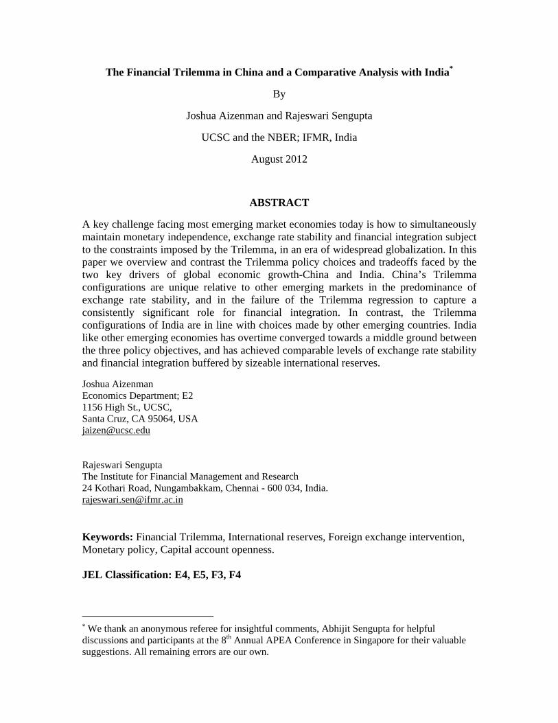
1. Introduction

The Great Recession that originated in 2008 has raised questions about the current

international financial architecture as well as individual countries’ international

macroeconomic policies. Policy makers dealing with the current global crisis are

confronted with the “Impossible Trinity” or the “Trilemma”- a potent paradigm of open

economy macroeconomics, asserting that a country may not simultaneously target the

exchange rate, conduct an independent monetary policy, and have full financial

integration. A key message of the Trilemma is scarcity of policy instruments. Policy

makers face a tradeoff, wherein increasing one Trilemma variable (for e.g. higher

financial integration) induces a drop in the weighted average of the other two variables

(i.e. lower exchange rate stability, or lower monetary independence, or a combination of

the two). Analyzing and understanding the predictions of the Trilemma hypothesis under

such mixed or hybrid regimes has now become a key challenge to policy makers and

practitioners alike, especially as countries all over the world recover from the effects of

the Great Recession.1

The rapid as well as massive financial globalization of most countries of the world

over the past 20 years, and the fast deepening of domestic and international financial

markets have modified the context of the Trilemma paradigm. Most emerging market

economies in particular have opted for increasing financial integration. The Trilemma

implies that a country choosing this path of higher capital mobility has to either forego

exchange rate stability if it intends to preserve certain degree of monetary independence,

or give up monetary independence if it wishes to retain exchange rate stability. As noted

in Aizenman, Chinn and Ito (2008), over the last couple of decades emerging market

economies have consistently pursued a balanced combination of the three

macroeconomic policy goals along with a substantial amount of international reserve (IR)

1 See Obstfeld, Shambaugh, and Taylor (2010) for further discussion and references dealing with the Trilemma, and Aizenman, Chinn and Ito (2008, 2010b, 2010c, 2011) for testing a continues version of the Trilemma tradeoffs. Related papers have discussed the possibility that a pegged exchange rate is a trap in the era of greater financial integration (e.g., Edwards and Levy-Yeyati, 2005; Aizenman and Glick, 2009).

3

holding. Emerging markets have mostly opted for hybrid exchange rate regimes -

managed exchange rate flexibility buffered by holding sizeable IR while increasing

financial integration and reducing the importance given to monetary independence. In

other words, among this group of countries, the three dimensions of the Trilemma

configurations: monetary independence, exchange rate stability, and financial openness,

are increasingly converging towards a “middle ground”.

All of these issues are highly pertinent in the context of the two major emerging

market economies, namely China and India. Economists, policymakers and practitioners

in recent debates and discussions, make an inevitable comparison between these two

rising giants in Asia, which together account for one third of the world population, and

also happen to be the world’s emerging super-powers displaying spectacular economic

ascent over the past couple of decades. While India is the eleventh largest economy by

nominal GDP, China occupies the second position surpassing Japan and after the US.

China and India are both large, poor countries facing similar challenges in

developing their economies and both have benefited from greater integration into the

world economy. In both countries, financial systems and markets were regulated and

controlled for a long period of time and were largely dominated by publicly owned

enterprises. In recent decades however, both countries have moved towards market-

driven economies through financial and trade liberalization. While economic

liberalization and deregulation policies were introduced in India in the 1990s, China

started receiving foreign direct investment from the mid-1980s onwards.

The similarities of India and China (their size, timing of takeoffs, and the

challenges facing them) raise important questions: Are these similarities reflected in the

macroeconomic Trilemma configurations adopted by China and India? What are the

implications of any differential choice of the Trilemma configurations made by these two

Asian giants? This paper attempts to address these issues using the framework of the

Trilemma and in the context of the macro history of China and India in the last two

decades.

China has been pursuing the objective of greater financial openness albeit more

cautiously than emerging economies elsewhere. As detailed in Glick and Hutchison

4

(2008), in order to deal with the Trilemma policy trade-offs, China has recently allowed

more exchange rate flexibility. However growing balance of payments surpluses through

both current and financial accounts have put upward pressure on its currency -- the

Renminbi. Chinese monetary authorities have been actively intervening in the foreign

exchange market thereby accumulating massive amounts of IR, so as to prevent the

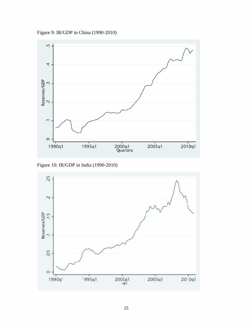
currency from appreciating. Between 1990 and 2010, China’s holdings of IR have risen

from close to $29 billion (8.3 percent of GDP) to over $2.8 trillion (close to 50 percent of

GDP).

As China continues to slowly liberalize its capital account while actively

intervening in the foreign exchange market to stabilize its currency, it faces the key

challenge of retaining domestic monetary policy autonomy and hence maintaining price

stability. In the recovery from the Great Recession of 2008-09, China has been facing

serious credit-boom fueled inflationary concerns. Chinese monetary authorities have

addressed this current challenge by raising banks’ reserve requirement ratios. However,

in the pursuit of higher financial openness and exchange rate stability, China is facing the

crucial trade-off of having to give up monetary policy independence. Clearly, the extent

to which China will successfully confront the Trilemma problem depends on achieving

the right balance of policy objectives.

India too fits the general pattern of most emerging market economies operating in a

range of partial financial integration and managed floating exchange rate regimes

accompanied by massive accumulation of IR. Following a balance of payments crisis in

1991, a comprehensive series of liberalization, privatization and deregulation policies

were implemented in the banking sector, trade sector as well as financial markets. Over

the next couple of decades the Indian economy witnessed several structural changes

(Shah, 2008; Mohan and Kapur, 2009; Hutchison, Sengupta, Singh, 2011). However,

with regard to capital account liberalization, Indian policy-makers adopted a cautious

stance from the very start (Hutchison, Kendall, Pasricha and Singh, 2010) as a result of

which the process has been a continuous albeit a slow and gradual one.

The Indian economy was among the first to recover from the global crisis of 2008-

09. While in the immediate aftermath of the crisis, capital outflows, higher exchange rate

5

volatility and loss of reserves to limit exchange rate depreciation presented a

contractionary influence on domestic monetary policy, the scenario has changed rapidly

in 2009-10 as capital inflows began surging again. (Hutchison, Sengupta, Singh, 2011).

Moreover, growing inflationary pressures (headline WPI inflation averaging around 10

percent) have forced the Reserve Bank of India (RBI) to resort to rate hikes and hence

adopt a tighter monetary policy. The RBI now clearly faces the challenge to strike a

balance between maintaining exchange rate stability and regaining monetary autonomy in

the face of growing capital inflows. All these economic developments and structural

changes, both in domestic and international environments may surely be expected to

influence the effective policy tradeoffs between the Trilemma choices facing the Indian

policy makers.

In this paper, we trace the evolution of the Financial Trilemma in China and India

over time from 1990 to 2010 and analyze the extent of the tradeoffs faced by policy

makers in both countries, between financial integration, monetary independence and

exchange rate stability. We calculate a Trilemma index for each of the two countries

separately using a methodology developed for a cross-section of countries by Aizenman,

Chinn and Ito-henceforth ACI (2008, 2010a, b and c, 2011). We also analyze the impact

of the evolving Trilemma configurations on macroeconomic indicators such as inflation

and examine the role of international reserves in the context of China and India’s

Trilemma.

We find that China’s Trilemma configurations are unique relative to the one

characterizing other emerging markets in the predominance of exchange rate stability and

in the failure of the Trilemma regression to capture any consistently significant role for

financial integration. One possible interpretation is that the fragmentation of the domestic

capital market in China, its array of capital controls and the large hoarding of IR imply

that the “policy interest rate” does not reflect the stance of monetary policy. In contrast,

the Trilemma configurations of India are in line with the regression results of other

emerging countries as reported in ACI (2008) and are consistent with the predictions of

the Trilemma tradeoffs. India like other emerging economies has overtime converged

towards a middle ground between the three policy objectives (i.e. increased financial

6

integration, managed exchange rate flexibility and active monetary policy) buffered by

sizeable international reserves.

2. Data and Methodology

We follow the methodology of ACI (2008, 2010a, b and c, 2011), henceforth ACI, in

constructing indices for each of the Trilemma policy objectives, namely, monetary

independence, exchange rate stability and capital account openness. However, while ACI

analyze the Trilemma configurations for a host of countries and study the implications

thereof, we do so individually for two key emerging market economies, namely China

and India and compare our results. In order to have more observations in our dataset and

hence more time variation for a single country, we use quarterly data as opposed to

annual data used in their analysis. We also use a different measure of capital account

openness than ACI.

For China, our data set extends from 1990Q1 to 2010Q4 spanning as many as 84

quarters. For the monetary independence index, we use weekly data on the lending rates

in China and 3-month LIBOR rates in US to compute quarterly correlations, as described

in the next sub-section. For the exchange rate stability index, we use the weekly series of

Renminbi-Dollar exchange rates to compute quarterly standard deviations, again as

delineated in the next subsection. All above-mentioned data are obtained from the

International Financial Statistics (IFS) database of the International Monetary Fund. In

order to compute the capital openness index we use data from the State Administration of

Foreign Exchange (SAFE) on outward and inward FDI, Portfolio and Other types of

capital flows as well as GDP data from IFS. Later on, for calculating China’s inflation

rate, we use consumer price index (CPI) data from Global Financial Statistics and

compute the YoY inflation rate using the quarterly CPI data. Finally to examine the

impact of IR we use quarterly data on foreign exchange reserves minus gold, from IFS

and normalize it by quarterly GDP.

For India, our data ranges from 1990Q1 to 2010Q4. For the Trilemma indices, we use

quarterly data on GDP, foreign investment inflows and outflows, from the International

7

Financial Statistics (IFS) database of the IMF. Same as for China, we use weekly

exchange rate series to construct a quarterly index of exchange rate stability, as described

below. The weekly, nominal Rupee-to-US dollar exchange rate series is from the Global

Financial Database. From the same source, we use weekly 90-day rates on

government/treasury securities for the US and India to calculate quarterly correlations

used to create the monetary independence index. Later on we use quarterly data on

wholesale price index (WPI) to calculate YoY inflation and data on foreign exchange

reserves minus gold to analyze the impact of reserves management and Trilemma indices

on inflation, both series obtained from the IFS database.

The monetary independence (MI), exchange rate stability (ES) and capital account

openness (KO) indices are constructed as follows for each of the two countries and each

index has been rescaled to lie between 0 and 1.2

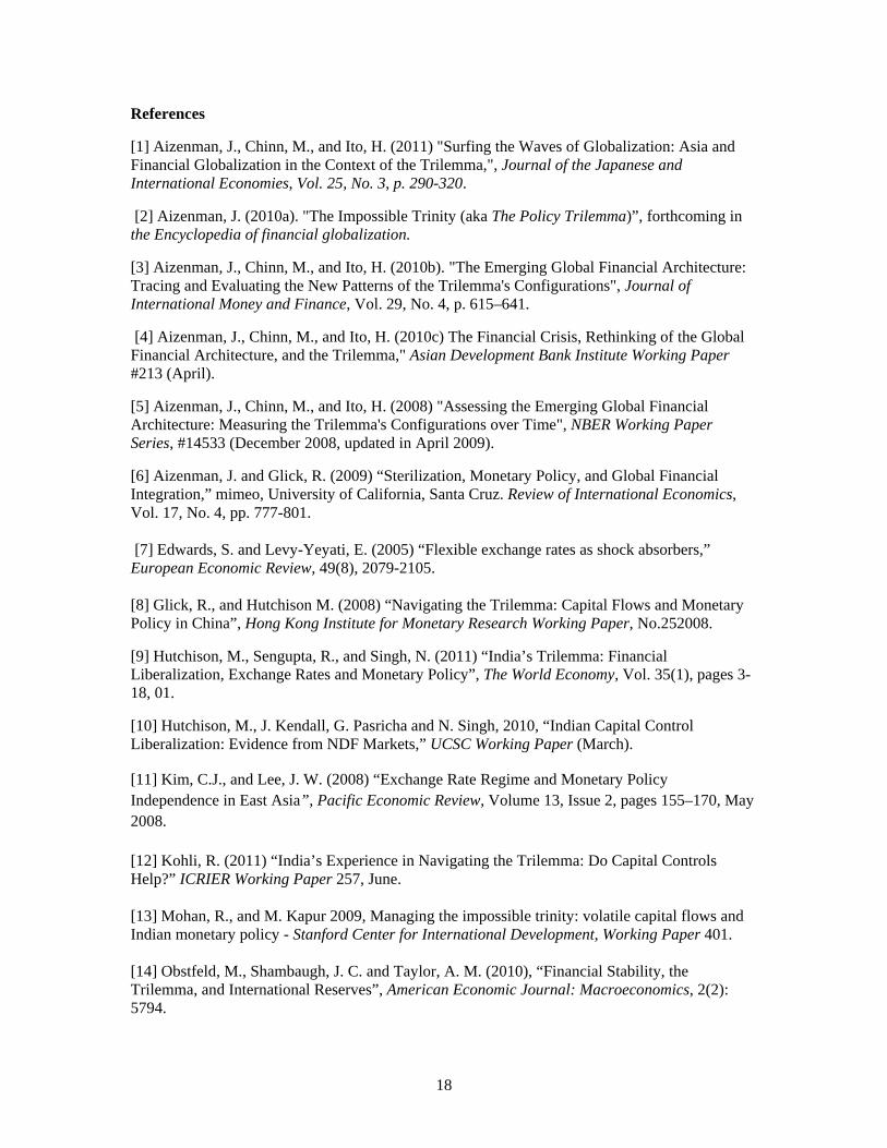
MI Index

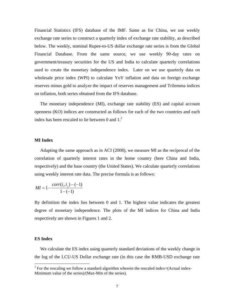
Adapting the same approach as in ACI (2008), we measure MI as the reciprocal of the

correlation of quarterly interest rates in the home country (here China and India,

respectively) and the base country (the United States). We calculate quarterly correlations

using weekly interest rate data. The precise formula is as follows:

( , ) ( 1)1

1 ( 1)i jcorr i i

MI

By definition the index lies between 0 and 1. The highest value indicates the greatest

degree of monetary independence. The plots of the MI indices for China and India

respectively are shown in Figures 1 and 2.

ES Index

We calculate the ES index using quarterly standard deviations of the weekly change in

the log of the LCU-US Dollar exchange rate (in this case the RMB-USD exchange rate

2 For the rescaling we follow a standard algorithm wherein the rescaled index=(Actual index-Minimum value of the series)/(Max-Min of the series).

8

for China and the Rupee-USD exchange rate for India). The formula used for the

construction of the index is as follows:

Like the MI Index, by definition the ES index ranges from 0 to 1 and the higher the value

the greater is the exchange rate stability. The evolution of the ES indices for China and

India during our sample period is shown in Figures 3 and 4, respectively.

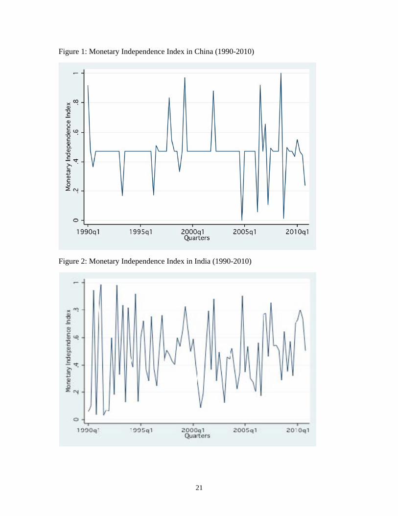
KO Index

We depart from ACI (2008) for the construction of the KO index in that instead of

using the Chinn-Ito index (that gives a number between 0 and 1 for a country’s financial

openness), we use a simple de-facto measure of capital account openness. We define the

KO index as the ratio of the sum of inward and outward foreign investment flows to

GDP, and we consider three types of capital flows-FDI, Portfolio and Others, as reported

by SAFE for China and the IFS for India.

During our sample period, slow and gradual changes have been taking place as

regards the capital account openness policy of both China and India and the Chinn-Ito

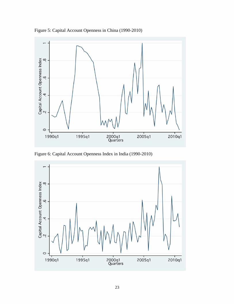
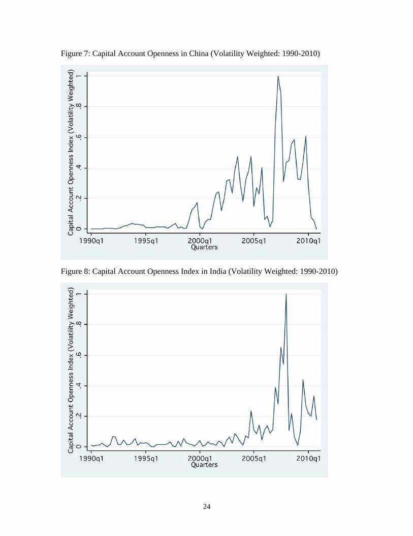
index may not necessarily capture these continuous changes very well. As a robustness

check, we also construct a second KO index measure wherein we weigh the different

types of capital flows by their respective annual volatility. One drawback of our measures

is that the KO indices are not bound between 0 and 1 by construct. In order to resolve this

issue we rescale both un-weighted and volatility-weighted measures of the KO index

[rescaled index=(Actual index-Minimum value of the series)/(Max-Min of the series)]

such that the indices lie between 0 and 1 and hence are comparable in values to the other

two indices, namely MI and ES. The time-series evolution of the KO indices using both

the weighted and un-weighted definitions for China and India have been presented in

Figures 5-8. All data details and descriptions have been presented in a Table in the

Appendix.

9

The Trilemma represents a binding trade-off between three policy objectives.

Accordingly, the main principle governing the methodology of the Trilemma estimation

is that an increase in any one of the three indices has to be balanced by a corresponding

decrease in one or two of the other indices, so that the constraint can be a binding one.

However, policy makers can choose to attain a combination of the three policy goals as

well subject to the constraint that neither of the indices reaches its maximum value. If all

three goals are simultaneously desirable, then whichever index has a higher value

represents the policy objective that authorities or central bankers want to focus on more.

This principle can be empirically captured using the methodology from ACI (2008).

Since there is no specific functional form of the policy trade-offs or the linkages

of these three policy goals, following ACI (2008) we test the simplest functional

specification for the three Trilemma indices and examine whether the three Trilemma

policy goals are linearly related. Thus the approach we use here for the estimation is to

regress a constant (in our case, two) on all three indices at the same time, omitting the

constant term on the right hand side of the regression equation. Specifically we examine

the goodness of fit of the following linear regression:

2 ai(MI)it bi(ES)it ci(KO)it it (1) where i= China or India. The estimated coefficients in the above regression should give

us some approximate ideas regarding the weights attached by policy makers to the three

policy goals. Moreover, if we find that the goodness of fit for the above regression model

is high, it would suggest that a linear specification is rich enough to explain the trade off

faced by policy makers among the three policy objectives. Thus, unlike ACI (2008), here

we use a time series for a single country to estimate the Trilemma configurations.

Both China and India underwent several changes in their respective exchange rate

regimes during the sample period. So apart from the baseline estimations for the full

sample, we also identify four sub-periods for each of the two countries and then estimate

equation (1) for each sub-period as an additional analysis. In the case of China, between

December 1989 and end of 1993, Chinese RMB went through a phase of devaluation.

Then on January 1994, official and swap markets were unified which amounted to a

10

massive devaluation against the USD. 1994 was an important break point in the exchange

rate regime, based on actual events rather than statistical tests so far and thus the first

sub-period we identify is 1990Q1-1994Q1. When the two rates were unified in 1994, the

currency was revalued till October 1997. Accordingly the second sub-period is 1994Q2-

1997Q4. From November 1997 to July 2005 (before the initiation of the reforms), RMB

fluctuated vis-à-vis USD in a very narrow range. So the third sub-period that we identify

is 1998Q1-2005Q3. In July 2005, China switched to a new exchange rate regime wherein

the rate was set with reference to a basket of currencies thereby signifying a shift away

from a dollar peg. The currency was allowed to ‘float’ more freely. Accordingly the final

sub-period is 2005Q4-2010Q4.

In the case of India the changes in exchange rate regime were relatively less

prominent. So we split the sample into four equal sub-periods roughly coinciding with

some regime changes as explained in Shah, Patnaik, Sethy and Balasubramaniam (2011).

The four sub-periods are 1990Q1-1995Q1, 1995Q2-2000Q2, 2000Q3-2005Q3 and

2005Q4-2010Q4.

According to ACI (2008), policymakers in emerging economies balance the

different trade-offs presented by the Trilemma in the short run through their reserve

management policies. In other words, they view reserves as a fourth dimension of these

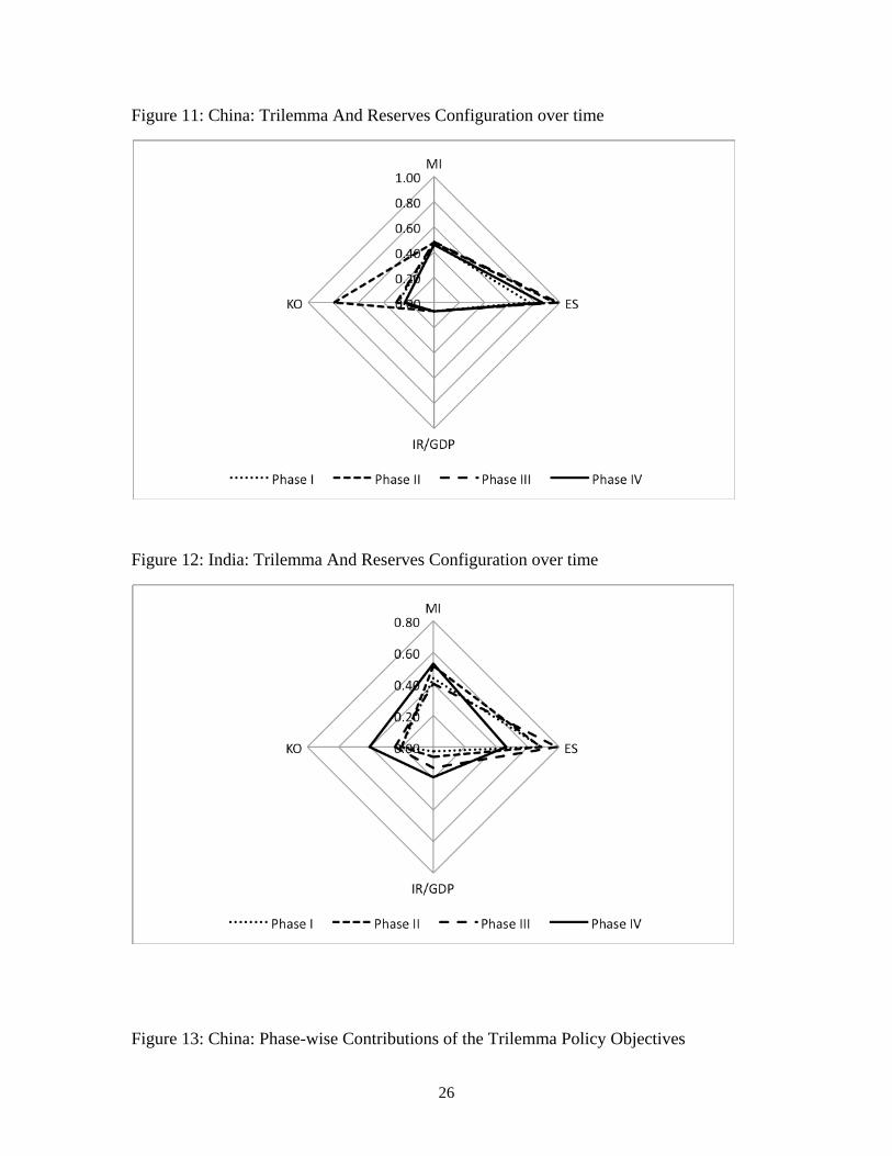
policy-trade offs. In Figures 11 and 12 we present the evolution of different

configurations of the Trilemma policy objectives for China and India respectively, along

with their reserves to GDP ratios, over the sub-periods. For each country we plot the

averages of each index over each sub-period using the ‘diamond chart’ popularized by

ACI (2008). Figure 11 shows that over time China’s policy stance has become more and

more skewed towards the ES objective at the expense of KO and especially MI. On the

other hand Figure 12 demonstrates that India over time has moved more towards the

middle of the diamond implying that like EMEs, India has been balancing all three policy

objectives and attaining a somewhat middle-ground perhaps through changes in its

reserves stock.

Estimation results for both countries are reported in Tables 1-4 and results are

discussed in detail in the next section.

11

3.1 Empirical Results: Trilemma Policy Stance

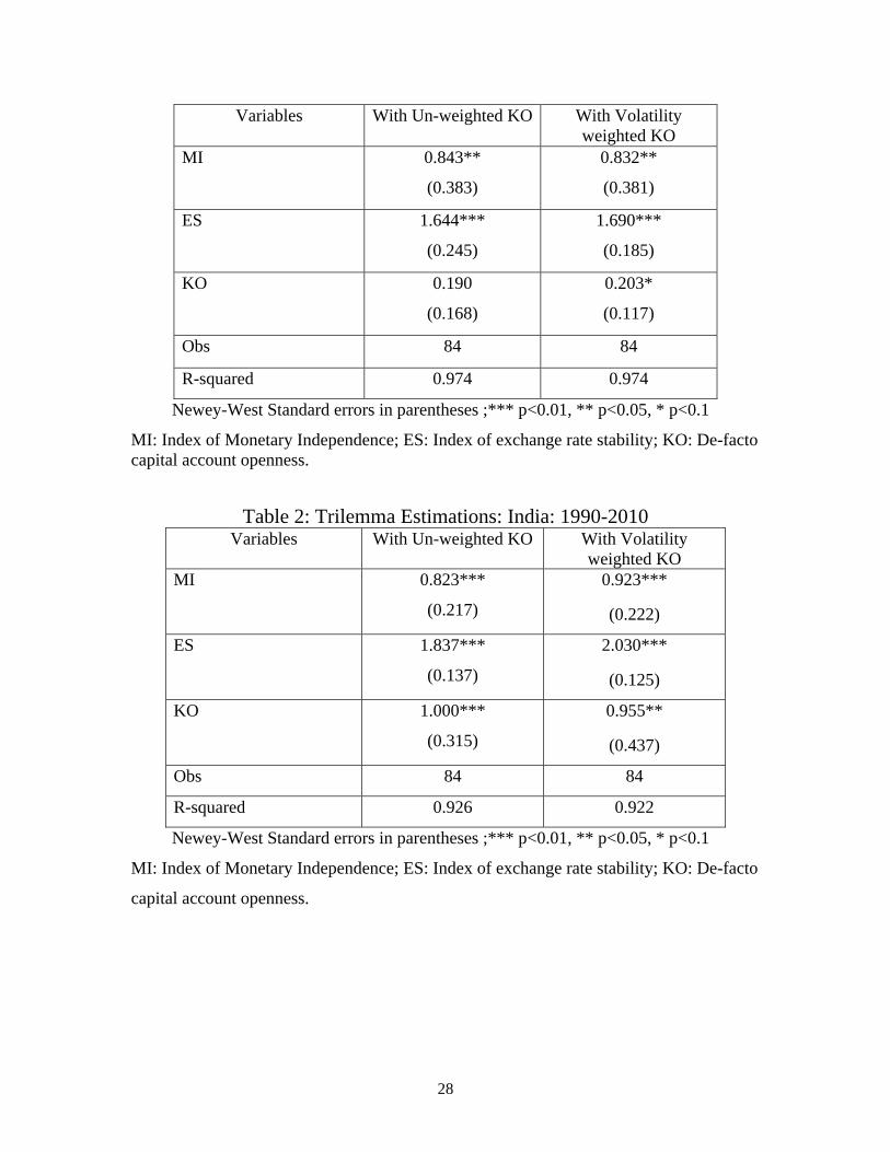
The baseline estimation results for China are reported in Table 1. In Column 1 we use

the KO index as defined in the previous section. In Column 2 of Table 1, we use a

weighted version of the KO index wherein the different types of capital flows (FDI,

portfolio and others) are weighted by their respective volatilities. In both regressions the

the estimated coefficients of the ES index are statistically significant and also have higher

magnitudes than the other two indices implying that China has clearly been placing more

priority on minimizing exchange rate fluctuations as a tool for macroeconomic

management. While the MI index also has statistically significant coefficients, the weight

attached to it is clearly less than the ES index as seen from the size of the coefficients.

Capital account openness does not come out to be statistically significant in our baseline

estimation in Column 1 and is only marginally significant at 10% level in Column 2. The

overall model-fit is also extremely good as reflected in the high R-squared numbers.3 The

adjusted R-squared is found to be above 98 percent, which indicates that the three policy

goals are linearly related to each other, that is, policy makers in China do indeed face the

trade-off among the three policy goals.

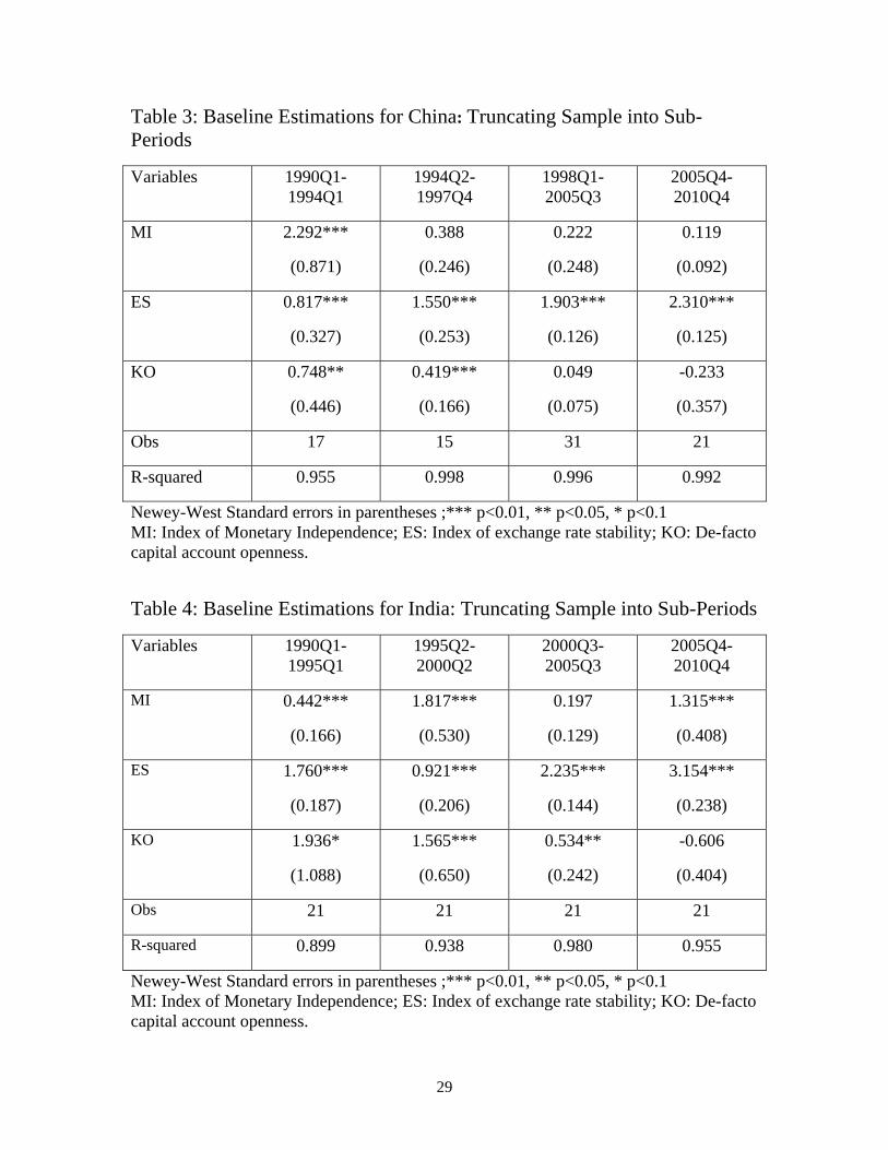
The predominance of exchange rate stability as a policy objective becomes even

more prominent when we look at the sub-periods in Table 3. Once again the one result

that stands out in Table 3 across all sub-periods is the consistent statistical significance of

the ES index compared to the other two indices. The exchange rate stabilization objective

has also been given more policy weight perhaps at the behest of monetary independence

and capital account openness.

We now turn to the baseline estimation results for India in Table 2 wherein

Columns 1 and 2 show estimation results using the un-weighted and volatility-weighted

KO indices respectively. The findings are strikingly different than China. All three

indices are consistently and statistically significant in the regressions in both Columns 1

and 2. Going by the size of the estimated coefficients, exchange rate stability and

financial integration are given marginally more importance followed by monetary

autonomy. These results for India are overall consistent with those found in ACI (2008)

3 Since there is no constant term on the right hand side, the R-squared is non-centered.

12

for a broader group of EMEs. Among this group the policy combination of exchange rate

stability and financial openness has been the most dominant over the past two decades.

The results in Table 4 also point at similar conclusions. All three policy objectives come

out significant for India with relatively higher weight being placed on the ES index.

Putting the regression results in the broader perspective, China’s Trilemma

configurations are unique relative to the one characterizing other emerging countries both

in the predominance of exchange rate stability, and in the failure of the Trilemma

regression to capture a consistently significant role for financial integration. In contrast,

the Trilemma configurations of India are in line with the regression results of ACI (2008,

2010a, b and c, 2011), and are consistent with the predictions of the Trilemma tradeoffs.

One possible interpretation is that the fragmentation of the domestic capital market in

China and the capital controls applied there implies that the “policy interest rate” is not

reflective of the stance of monetary policy. This would be the case if a large share of

borrowing is allocated directly by the state banking system, with preferential treatment of

the state owned enterprises (SOE), and if the supply of credit to the private sector is

segmented. Another unique feature of China is a combination of more stringent capital

controls and massive hoarding of IR. China has been increasing its IR/GDP relentlessly

without signs of convergence to a target IR/GDP during the sample period. These

policies may relax the Trilemma constraints in the intermediate run, as is suggested by

ACI (2010b, c and d). Furthermore, the emergence of endogenous capital flows

circumventing the controls in China (including trade mis-invoicing) may reduce the

explanatory power of the Trilemma variables in China. Needless to say, these conjectures

need further investigations.

In contrast, the Trilemma configurations of India and the tradeoffs among the

policy goals there are in line with the results of other emerging markets. This is reflected

both by the significant positive sign of the Trilemma variables, and by the “middle

ground” choices of India, in line with the trend among most other emerging economies

[see ACI (2010a, b and c)]. Overtime the Trilemma configuration that has evolved in

India is one of greater exchange rate stability and financial integration, combined with an

13

attempt to retain monetary autonomy through active intervention in foreign exchange

markets.

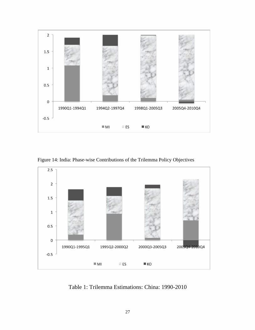
We also graphically demonstrate the contributions of the Trilemma policy

objectives over time, for both China and India in Figures 13 and 14 respectively.4 Once

again for China, it is clearly evident that exchange rate stability has been assigned the

maximum weight in the Trilemma trade-offs whereas in India, over time, all three policy

objectives seem to matter in the overall trade-off. The contributions add up to almost to

two (trilemma constant) for both countries in each sample period implying relatively high

goodness of fit of the model estimated.

3.2 Empirical Results: Trilemma and Inflation

In this section we examine econometrically how various choices regarding the

three policies affect inflation in both China and India. Inflation is a leading indicator of

macroeconomic stability.5 The effect on inflation of the various Trilemma policy choices,

independently as well as in conjunction with international reserves can throw some useful

insights on how to manage inflation. This is especially pertinent in recent times since

both China and India are now confronted with serious domestic inflationary pressures.

Given this, we empirically explore the linkages between inflation and our time-varying

measures of the policy goals associated with the Trilemma configuration. In particular we

estimate the following model:

(2)

where, yit is a measure for YoY inflation calculated using quarterly data, for country i

(China or India) in year t.6 TLMit is a vector of any two of the three Trilemma indices,

4Contributions are measured by multiplying the estimated coefficient of each index from Tables 3 and 4 with the respective series average for each sub-period. 5While ACI (2008) also look at the effect of Trilemma on output volatility, for our study output data is not available for sufficiently high frequencies to allow construction of a quarterly output volatility series for individual countries. That is another reason why we focus on inflation alone.6 While consumer price index is used for China, in case of India we use the wholesale price index to calculate inflation.

14

namely, MI, ES, and KO. (IR/GDP)it is the level of international reserves (excluding gold)

as a ratio to GDP. [TLMit x (IR/GDP)it] is an interaction term between the Trilemma

indices and the IR/GDP. Xit is a vector of country-specific determinants of inflation such

as output growth rate (quarterly growth rate of real GDP) and money growth rate

(quarterly growth rate of money supply or M1). The effect of the interaction terms will

help to identify whether IR complement or act as a substitute for other policy stances.7

Our objective is to analyze the impact of the evolving Trilemma configurations on

domestic inflation in both countries and to investigate how has the surge in IR

accumulation affected this macroeconomic policy dynamics.

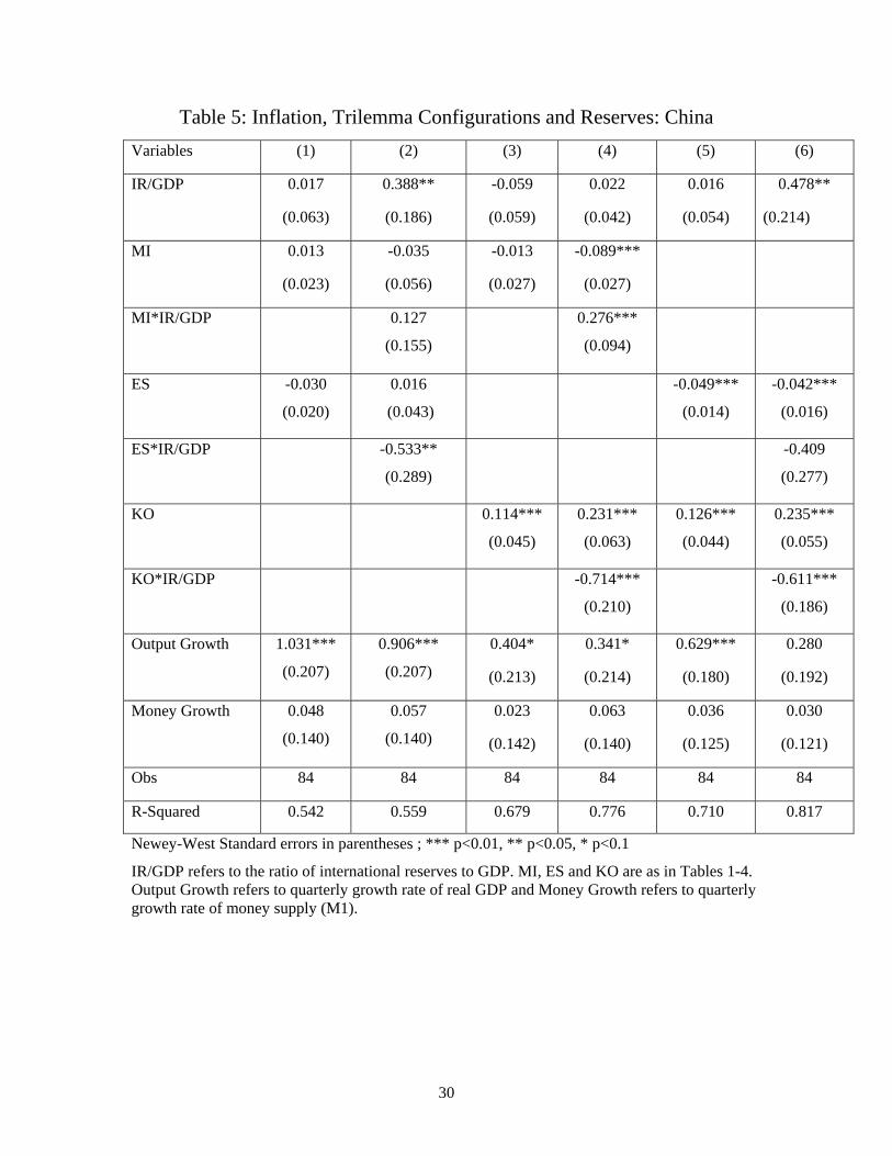
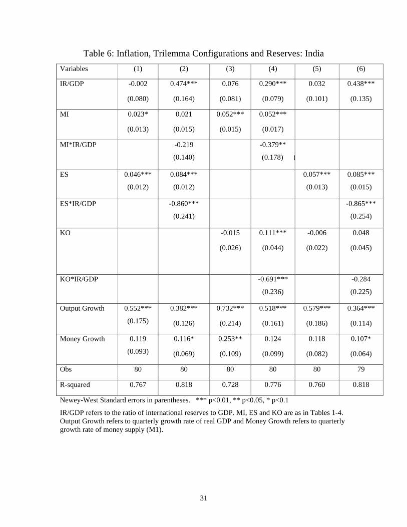
Results of the estimation are reported in Tables 5 and 6 respectively for China and

India. In case of China, higher IR/GDP increases inflation at a rate that increases with

MI. If IR/GDP is 0.5, the net coefficient on MI for China is 0.045 (0.27*0.5 - 0.09),

positive, yet it is negative for IR/GDP of 0.2. This suggests that high IR hoarding may

induce inflationary pressure with a given MI. It also seems that throughout most of the

sample, both countries managed to sterilize effectively, preventing spillover effects from

hoarding international reserves to domestic prices. This is reflected in the insignificant

coefficient of the IR/GDP in columns 1, 3 and 5, in the baseline regressions with no

interaction terms in both Tables 5 and 6. Adding the interaction terms does not change

this result much. While the direct effect of IR/GDP is positive, evaluating the marginal

impact of increasing IR/GDP on inflation, conditioning it on the sample levels of MI, ES,

and KO indicates that the marginal impact of higher IR/GDP was close to nil.8 This

result may reflect the financial repression stance of both countries, where the authorities

occasionally adjusted banks’ reserve/deposit rates at times of abundance liquidity. Yet,

this result should be taken with a grain of salt, as it reflects the average patters observed

during sample period, and thereby is backward looking. As IR/GDP trends upwards in

both countries, reaching more than 50 percent in China, past experience does not

guarantee the success of future sterilization. 7 Since output data is not available for sufficiently high frequencies to allow construction of a quarterly output volatility series, we focus on inflation alone. 8 To illustrate, note that column 2 implies that . Substituting the sample averages of the Trilemma indices into the regression results suggests that the marginal effect of raising IR/GDP on the inflation was practically nil.

15

In the case of China, monetary independence seems to have no statistically

significant effect on inflation. However, greater exchange rate stability, as well as capital

market openness, seem to have come at the cost of higher inflation. This may reflect the

real exchange rate appreciation induced by the rapid growth of the Chinese economy,

where nominal exchange rate stability induces higher inflation rate. This interpretation

suggests that greater exchange rate flexibility, allowing nominal appreciation, would

reduce inflation in China. This view is consistent with the long run neutrality of

exchange rate regimes. In a fast growing economy, a choice in favor of exchange rate

stability overtime shifts the adjustment to appreciating real exchange rate from the

nominal exchange rate appreciation to the domestic inflation.

For India, on the other hand, monetary autonomy is positively related to inflation.

Similarly to China, greater exchange rate stability has been associated with higher

inflation, possibly again due to the real exchange rate appreciation associated with rapid

growth. Capital account openness does not seem to have a major effect on inflation in this

case. It is possible that greater ES may have been adopted to reduce inflation in future

periods. Also to be noted that if IR/GDP in India is 0.15, the net effect of ES on inflation

is positive (0.1*1.5-1). Similarly, MI will increase inflation if there is no attempt to use

MI to target a low inflation. Once again capital account openness is associated with

higher inflation. A surge of capital inflows may often lead to overheated asset prices in

the stock market as well as in the real estate sector, which in turn could feed, into

inflation. On the other hand, if the capital inflows are absorbed into higher reserve

accumulation through sterilized intervention by the RBI in the foreign exchange market,

then the transmission into higher prices is likely to be subdued—this could explain the

significant, negative coefficient of the interaction term between KO and IR/GDP in the

case of both China and India.

4. Concluding Remarks

A key challenge facing most emerging market economies today is how to

simultaneously maintain monetary independence, exchange rate stability and financial

integration subject to the constraints imposed by the Financial Trilemma, in an era of

16

deepening globalization. In this paper we study the Trilemma choices of the two key

drivers of global growth, China and India which together account for one third of the

world population, rank among the front-runners of the global economy and are among the

biggest and fastest growing developing countries. Their success stories are defined by

consistently high growth rates of both aggregate and per capita incomes in recent

decades, competing aggressively in the global markets.

We overview and contrast the policy choices followed by these two countries

during 1990-2010 and empirically test their Trilemma tradeoffs. We calculate a Trilemma

index for each of the two countries separately, analyze the impact of the evolving

Trilemma configurations on macroeconomic indicators such as inflation and examine the

role of international reserves in the context of their Trilemma. We find that China’s

Trilemma configurations are quite unique relative to the one characterizing other

emerging markets. China has clearly been placing more priority on minimizing exchange

rate fluctuations as a tool for macroeconomic management during the period of our

analysis. The predominance of exchange rate stability has been achieved to some extent

at the expense of monetary autonomy and financial integration. On the other hand, we

find that India has overtime converged towards a middle ground between the three policy

objectives, and has achieved comparable levels of exchange rate stability and financial

integration buffered by sizeable international reserves.

The comparative Trilemma analysis of China and India as presented here is quite

pertinent in the current global economic scenario. The Global Financial Crisis proved the

short-run resilience of both countries-the two fastest growing economies that kept the

global growth engine moving despite stagnation in the developed world. However in

recent times both countries seem to be facing significant domestic economic challenges

as well as adverse external shocks originating from the Euro zone slow down.

In the aftermath of the Global Financial Crisis, India is struggling to deal with its

fiscal and current account deficits as well as a high domestic inflation rate. In 2010,

annual average whole-sale price inflation was as high as 10.2 percent. The Reserve Bank

of India has been raising interest rates consistently since November 2010 to counter

inflation that went into the double digits fueled by growing consumer demand and

17

increasing food and fuel prices. Growth has also slowed down significantly from 9% to

6% in the last 2 years. China on the other hand is grappling with slowing exports given

the global economic slowdown. Uncertainty is also looming large about the growing non-

performing loans in the domestic banking system. Against this background, it will be

interesting to see how the Trilemma policy trade-offs evolve for both these economies in

the years to come, especially as the global economy recovers from the Great Recession.

18

References

[1] Aizenman, J., Chinn, M., and Ito, H. (2011) "Surfing the Waves of Globalization: Asia and Financial Globalization in the Context of the Trilemma,", Journal of the Japanese and International Economies, Vol. 25, No. 3, p. 290-320.

[2] Aizenman, J. (2010a). "The Impossible Trinity (aka The Policy Trilemma)”, forthcoming in the Encyclopedia of financial globalization.

[3] Aizenman, J., Chinn, M., and Ito, H. (2010b). "The Emerging Global Financial Architecture: Tracing and Evaluating the New Patterns of the Trilemma's Configurations", Journal of International Money and Finance, Vol. 29, No. 4, p. 615–641.

[4] Aizenman, J., Chinn, M., and Ito, H. (2010c) The Financial Crisis, Rethinking of the Global Financial Architecture, and the Trilemma," Asian Development Bank Institute Working Paper #213 (April).

[5] Aizenman, J., Chinn, M., and Ito, H. (2008) "Assessing the Emerging Global Financial Architecture: Measuring the Trilemma's Configurations over Time", NBER Working Paper Series, #14533 (December 2008, updated in April 2009).

[6] Aizenman, J. and Glick, R. (2009) “Sterilization, Monetary Policy, and Global Financial Integration,” mimeo, University of California, Santa Cruz. Review of International Economics, Vol. 17, No. 4, pp. 777-801. [7] Edwards, S. and Levy-Yeyati, E. (2005) “Flexible exchange rates as shock absorbers,” European Economic Review, 49(8), 2079-2105. [8] Glick, R., and Hutchison M. (2008) “Navigating the Trilemma: Capital Flows and Monetary Policy in China”, Hong Kong Institute for Monetary Research Working Paper, No.252008.

[9] Hutchison, M., Sengupta, R., and Singh, N. (2011) “India’s Trilemma: Financial Liberalization, Exchange Rates and Monetary Policy”, The World Economy, Vol. 35(1), pages 3-18, 01.

[10] Hutchison, M., J. Kendall, G. Pasricha and N. Singh, 2010, “Indian Capital Control Liberalization: Evidence from NDF Markets,” UCSC Working Paper (March).

[11] Kim, C.J., and Lee, J. W. (2008) “Exchange Rate Regime and Monetary Policy Independence in East Asia”, Pacific Economic Review, Volume 13, Issue 2, pages 155–170, May 2008. [12] Kohli, R. (2011) “India’s Experience in Navigating the Trilemma: Do Capital Controls Help?” ICRIER Working Paper 257, June. [13] Mohan, R., and M. Kapur 2009, Managing the impossible trinity: volatile capital flows and Indian monetary policy - Stanford Center for International Development, Working Paper 401. [14] Obstfeld, M., Shambaugh, J. C. and Taylor, A. M. (2010), “Financial Stability, the Trilemma, and International Reserves”, American Economic Journal: Macroeconomics, 2(2): 5794.

19

[15] Patnaik, I., A. Shah, A. Sethy, and V. Balasubramaniam. (2011), “The exchange rate regime in Asia: From crisis to crisis”, International Review of Economics and Finance, 20, 32-43. [16] Shah, A., 2008, New issues in Indian macro policy. In T. N. Ninan, editor, Business Standard India. New Delhi: Business Standard Books. [17] Sokolov, V., Lee, B.J., and Mark, N. (2011) “Linkages between Exchange Rate Policy and Macroeconomic Performance”, Pacific Economic Review, Volume 16, Issue 4, pages 395–420.

20

Appendix: Data Details and Sources Variable Name Description Components Data Sources

MI Monetary Independence Index: As defined in Text

Domestic and US interest rates

China: Weekly Lending rates from International Financial Statistics Database (IFS)

India: Weekly 90-day rates on government securities from Global Financial Database (GFD)

Interest rate (USA): 3 month LIBOR from IFS

ES Exchange Rate Stability: As defined in Text

Domestic Exchange Rate (LCU/USD)

China: Weekly RMB/USD exchange rate from IFS.

India: Weekly Rupee/USD exchange rate from GFD.

KO Capital Openness Index: Sum of Capital Inflows and Outflows divided by GDP

FDI, Portfolio and Other inflows and outflows and GDP

China: Quarterly FDI, Portfolio and Other flows from the State Administration of Foreign Exchange (SAFE); GDP from IFS.

India: Foreign investment inflows and outflows from IFS.

Volatility-Weighted KO

Sum of each type of capital flows weighted by respective volatilities, divided by GDP

FDI, Portfolio and Other inflows and outflows and GDP

China: Quarterly FDI, Portfolio and Other flows from the State Administration of Foreign Exchange (SAFE); GDP from IFS.

India: Foreign investment inflows and outflows from IFS.

IR/GDP International Reserves to GDP Ratio

Foreign Exchange Reserves minus gold and GDP

Reserves and GDP from IFS

Inflation YoY Inflation calculated using quarterly price index data

Consumer Price Index for China and Wholesale Price Index for India

China: CPI from GFD

India: WPI from GFD

Output Growth Quarterly growth rate of real GDP

Nominal GDP, CPI and WPI

China: CPI from GFD; GDP from IFS

India: WPI from GFD; GDP from IFS

Money Growth Quarterly growth rate of money supply

M1 China and India: M1 from GFD

21

Figure 1: Monetary Independence Index in China (1990-2010)

Figure 2: Monetary Independence Index in India (1990-2010)

22

Figure 3: Exchange Rate Stability Index in China (1990-2010)

Figure 4: Exchange Rate Stability Index in India (1990-2010)

23

Figure 5: Capital Account Openness in China (1990-2010)

Figure 6: Capital Account Openness Index in India (1990-2010)

24

Figure 7: Capital Account Openness in China (Volatility Weighted: 1990-2010)

Figure 8: Capital Account Openness Index in India (Volatility Weighted: 1990-2010)

25

Figure 9: IR/GDP in China (1990-2010)

Figure 10: IR/GDP in India (1990-2010)

26

Figure 11: China: Trilemma And Reserves Configuration over time

Figure 12: India: Trilemma And Reserves Configuration over time

Figure 13: China: Phase-wise Contributions of the Trilemma Policy Objectives

27

Figure 14: India: Phase-wise Contributions of the Trilemma Policy Objectives

Table 1: Trilemma Estimations: China: 1990-2010

28

Variables With Un-weighted KO With Volatility weighted KO

MI 0.843**

(0.383)

0.832**

(0.381)

ES 1.644***

(0.245)

1.690***

(0.185)

KO 0.190

(0.168)

0.203*

(0.117)

Obs 84 84

R-squared 0.974 0.974

Newey-West Standard errors in parentheses ;*** p<0.01, ** p<0.05, * p<0.1

MI: Index of Monetary Independence; ES: Index of exchange rate stability; KO: De-facto capital account openness.

Table 2: Trilemma Estimations: India: 1990-2010 Variables With Un-weighted KO With Volatility

weighted KO MI 0.823***

(0.217)

0.923***

(0.222)

ES 1.837***

(0.137)

2.030***

(0.125)

KO 1.000***

(0.315)

0.955**

(0.437)

Obs 84 84

R-squared 0.926 0.922

Newey-West Standard errors in parentheses ;*** p<0.01, ** p<0.05, * p<0.1

MI: Index of Monetary Independence; ES: Index of exchange rate stability; KO: De-facto

capital account openness.

29

Table 3: Baseline Estimations for China: Truncating Sample into Sub-Periods

Variables 1990Q1-1994Q1

1994Q2-1997Q4

1998Q1-2005Q3

2005Q4-2010Q4

MI 2.292***

(0.871)

0.388

(0.246)

0.222

(0.248)

0.119

(0.092)

ES 0.817***

(0.327)

1.550***

(0.253)

1.903***

(0.126)

2.310***

(0.125)

KO 0.748**

(0.446)

0.419***

(0.166)

0.049

(0.075)

-0.233

(0.357)

Obs 17 15 31 21

R-squared 0.955 0.998 0.996 0.992

Newey-West Standard errors in parentheses ;*** p<0.01, ** p<0.05, * p<0.1 MI: Index of Monetary Independence; ES: Index of exchange rate stability; KO: De-facto capital account openness.

Table 4: Baseline Estimations for India: Truncating Sample into Sub-Periods

Variables 1990Q1-1995Q1

1995Q2-2000Q2

2000Q3-2005Q3

2005Q4-2010Q4

MI 0.442***

(0.166)

1.817***

(0.530)

0.197

(0.129)

1.315***

(0.408)

ES 1.760***

(0.187)

0.921***

(0.206)

2.235***

(0.144)

3.154***

(0.238)

KO 1.936*

(1.088)

1.565***

(0.650)

0.534**

(0.242)

-0.606

(0.404)

Obs 21 21 21 21

R-squared 0.899 0.938 0.980 0.955

Newey-West Standard errors in parentheses ;*** p<0.01, ** p<0.05, * p<0.1 MI: Index of Monetary Independence; ES: Index of exchange rate stability; KO: De-facto capital account openness.

30

Table 5: Inflation, Trilemma Configurations and Reserves: China

Variables (1) (2) (3) (4) (5) (6)

IR/GDP 0.017

(0.063)

0.388**

(0.186)

-0.059

(0.059)

0.022

(0.042)

0.016

(0.054)

0.478**

(0.214)

MI 0.013

(0.023)

-0.035

(0.056)

-0.013

(0.027)

-0.089***

(0.027)

MI*IR/GDP 0.127

(0.155)

0.276***

(0.094)

ES -0.030

(0.020)

0.016

(0.043)

-0.049***

(0.014)

-0.042***

(0.016)

ES*IR/GDP -0.533**

(0.289)

-0.409

(0.277)

KO 0.114***

(0.045)

0.231***

(0.063)

0.126***

(0.044)

0.235***

(0.055)

KO*IR/GDP -0.714***

(0.210)

-0.611***

(0.186)

Output Growth 1.031***

(0.207)

0.906***

(0.207)

0.404*

(0.213)

0.341*

(0.214)

0.629***

(0.180)

0.280

(0.192)

Money Growth 0.048

(0.140)

0.057

(0.140)

0.023

(0.142)

0.063

(0.140)

0.036

(0.125)

0.030

(0.121)

Obs 84 84 84 84 84 84

R-Squared 0.542 0.559 0.679 0.776 0.710 0.817

Newey-West Standard errors in parentheses ; *** p<0.01, ** p<0.05, * p<0.1

IR/GDP refers to the ratio of international reserves to GDP. MI, ES and KO are as in Tables 1-4. Output Growth refers to quarterly growth rate of real GDP and Money Growth refers to quarterly growth rate of money supply (M1).

31

Table 6: Inflation, Trilemma Configurations and Reserves: India

Variables (1) (2) (3) (4) (5) (6)

IR/GDP -0.002

(0.080)

0.474***

(0.164)

0.076

(0.081)

0.290***

(0.079)

0.032

(0.101)

0.438***

(0.135)

MI 0.023*

(0.013)

0.021

(0.015)

0.052***

(0.015)

0.052***

(0.017)

MI*IR/GDP -0.219

(0.140)

-0.379**

(0.178) (

ES 0.046***

(0.012)

0.084***

(0.012)

0.057***

(0.013)

0.085***

(0.015)

ES*IR/GDP -0.860***

(0.241)

-0.865***

(0.254)

KO -0.015

(0.026)

0.111***

(0.044)

-0.006

(0.022)

0.048

(0.045)

KO*IR/GDP -0.691***

(0.236)

-0.284

(0.225)

Output Growth 0.552***

(0.175)

0.382***

(0.126)

0.732***

(0.214)

0.518***

(0.161)

0.579***

(0.186)

0.364***

(0.114)

Money Growth 0.119

(0.093)

0.116*

(0.069)

0.253**

(0.109)

0.124

(0.099)

0.118

(0.082)

0.107*

(0.064)

Obs 80 80 80 80 80 79

R-squared 0.767 0.818 0.728 0.776 0.760 0.818

Newey-West Standard errors in parentheses. *** p<0.01, ** p<0.05, * p<0.1

IR/GDP refers to the ratio of international reserves to GDP. MI, ES and KO are as in Tables 1-4. Output Growth refers to quarterly growth rate of real GDP and Money Growth refers to quarterly growth rate of money supply (M1).