Middlesex University Research RepositoryAn open access repository of

Middlesex University research

http://eprints.mdx.ac.uk

Huyck, Christian R. ORCID: https://orcid.org/0000-0003-4015-3549 (2009) Variable binding bysynaptic strength change. Connection Science, 21 (4) . pp. 327-357. ISSN 0954-0091 [Article]

(doi:10.1080/09540090902954188)

This version is available at: https://eprints.mdx.ac.uk/4301/

Copyright:

Middlesex University Research Repository makes the University’s research available electronically.

Copyright and moral rights to this work are retained by the author and/or other copyright ownersunless otherwise stated. The work is supplied on the understanding that any use for commercial gainis strictly forbidden. A copy may be downloaded for personal, non-commercial, research or studywithout prior permission and without charge.

Works, including theses and research projects, may not be reproduced in any format or medium, orextensive quotations taken from them, or their content changed in any way, without first obtainingpermission in writing from the copyright holder(s). They may not be sold or exploited commercially inany format or medium without the prior written permission of the copyright holder(s).

Full bibliographic details must be given when referring to, or quoting from full items including theauthor’s name, the title of the work, publication details where relevant (place, publisher, date), pag-ination, and for theses or dissertations the awarding institution, the degree type awarded, and thedate of the award.

If you believe that any material held in the repository infringes copyright law, please contact theRepository Team at Middlesex University via the following email address:

eprints@mdx.ac.uk

The item will be removed from the repository while any claim is being investigated.

See also repository copyright: re-use policy: http://eprints.mdx.ac.uk/policies.html#copy

Journal …Connection Science Article ID … CCOS395590

TO: CORRESPONDING AUTHOR

AUTHOR QUERIES - TO BE ANSWERED BY THE

CORRESPONDING AUTHOR Dear Author Please address all the numbered queries on this page which are clearly identified on the proof for your convenience. Thank you for your cooperation Q1 Please confirm affiliation details. Q2 Please provide publisher location for the following

references: Abeles (1991), Amit (1989), Anderson and Lebiere (1998), Churchland and Sejnowski (1992), Dayan and Abbott (2005), Filmore (1968), Hebb (1949), Hofstadter (1979), Hopcroft and Ullman (1979), Jackendoff (2002), Klatzky (1980), Maass and Bishop (2001), Malsburg (1986), Newell (1990), Rumelhart and McClelland (1986), Schank and Abelson (1977), Shieber (1986), Wennekers and Palm (2000).

Q3 Please provide editors initials and publisher location for reference Braitenberg (1989).

Q4 Please provide more details for reference Huyck (2008, 2009).

Q5 Please provide page range for reference Sompolinsky (1987).

Production Editorial Department, Taylor & Francis 4 Park Square, Milton Park, Abingdon OX14 4RN

Telephone: +44 (0) 1235 828600 Facsimile: +44 (0) 1235 829000

0.8C

opye

dite

dby

:A

A

1234567891011121314151617181920212223242526272829303132333435363738394041424344454647484950

Connection ScienceVol. 00, No. 00, Month 2009, 1–31

Variable binding by synaptic strength change

Christian R. Huyck*

School of Computing Science, Middlesex University, The Burroughs, London, NW4 4BT, UK Q1

(Received 11 September 2008; final version received 7 April 2009 )

Variable binding is a difficult problem for neural networks. Two new mechanisms for binding by synapticchange are presented, and in both, bindings are erased and can be reused. The first is based on the commonlyused learning mechanism of permanent change of synaptic weight, and the second on synaptic change whichdecays. Both are biologically motivated models. Simulations of binding on a paired association task areshown with the first mechanism succeeding with a 97.5% F-Score, and the second performing perfectly.Further simulations show that binding by decaying synaptic change copes with cross talk, and can be usedfor compositional semantics. It can be inferred that binding by permanent change accounts for these, but itfaces the stability plasticity dilemma. Two other existing binding mechanisms, synchrony and active links,are compatible with these new mechanisms. All four mechanisms are compared and integrated in a CellAssembly theory.

Keywords: variable binding; cell assembly; short-term potentiation; long-term potentiation; synchrony;stability plasticity dilemma

1. Introduction

Symbol systems have been enormously successful and it has been proposed that, at least at somelevel, humans are symbol processors (Newell 1990). Whether humans are symbol processors ornot, they can effectively use rules, and symbolic systems, such as ACT (Anderson and Lebiere1998), have been very successful as models of human cognition. This success is probably due tothe rule based or at least rule-like behaviour of humans in a wide range of tasks such as naturallanguage processing.

Unfortunately, symbolic systems also have problems with brittleness (Smolensky 1987). Thesymbols are not grounded (Harnad 1990) and it is difficult or impossible to learn new sym-bols that are not just some combination of existing symbols (Frixione, Spinelli, and Gaglio1989).

These and other problems provided motivation for the rise of connectionism, particularly inthe 1980s. Connectionist systems are particularly good at learning, and thus may be able to learn

*Email: c.huyck@mdx.ac.uk

ISSN 0954-0091 print/ISSN 1360-0494 online© 2009 Taylor & FrancisDOI: 10.1080/09540090902954188http://www.informaworld.com

Techset Composition Ltd, Salisbury CCOS395590.TeX Page#: 31 Printed: 23/4/2009

51525354555657585960616263646566676869707172737475767778798081828384858687888990919293949596979899100

2 C.R. Huyck

new symbols. If the systems learn from an environment, the newly learned symbols might evenhave semantic content grounded in that environment.

However, early connectionist systems were criticised for their inability to perform symbolicprocesses (Lindsey 1988). In particular, they were criticised for their lack of compositional syntaxand semantics (Fodor and Pylyshyn 1988).

Variable binding offers an answer to these criticisms.A good variable binding solution allows forthe implementation of rules; connectionist primitives can be combined, and variables instantiatedas constants. If this can be done so that the result has compositional syntax and semantics, thecriticism will have been answered.

For a binding mechanism to be functional, it must be able to support a range of bindingbehaviours (Section 2.1). Binding by synchrony (Malsburg 1981) is a well explored mechanismthat is functional, but it can only support a limited number of bindings. Similarly, binding byactive links (van der Velde and de Kamps 2006) has also been explored and is functional. Bothmechanisms are restricted to active bindings, that is, the bindings must be continuously supportedby neural firing, and when that firing ceases so do the bindings. This may limit the effectivenessof a neural system, particularly as it relates to composition (Section 6.2).

After some background for reader orientation, binding by synaptic change is introduced. Thiscomes in two forms, binding by short-term potentiation (STP) and binding by compensatory long-term potentiation (LTP). Simulations that indicate these mechanisms are functional are described,in particular showing bindings can be formed and erased, that bindings can overlap, that a largenumber of bindings can be supported simultaneously, and that they can provide compositionalsyntax and semantics. It is shown that the four binding mechanisms, two existing and the twonovel synaptic change mechanisms, are not mutually exclusive, and one system could use all fourmechanisms. Ramifications for memory formation speed and duration are also explored alongwith other issues in the discussion and conclusion.

2. Background

Humans behave as if they have compositional syntax and semantics, so if systems based solely onneural models are to duplicate human behaviour, they too must exhibit compositional syntax andsemantics behaviour. One way for neural systems to exhibit compositional syntax and semanticsis by variable binding.

A good cognitive model should have compositional syntax and semantics (Fodor and Pylyshyn1988). Standard symbolic cognitive architectures have this compositionality, but it is more difficultfor connectionist models to exhibit it.

Compositional semantics means that the semantics of a complex thing includes the semanticsof that thing’s constituents. So sentence 1

Pat loves Jody. Sentence 1Includes the semantics of Pat, love, and Jody. Compositional syntax means that the syntacticstructure of complex things affects the underlying semantics. For example, the semantics ofsentence 1 is different from the semantics of sentence 2.

Jody loves Pat. Sentence 2So the semantics of a sentence must be more than the sum of its parts.

Variable binding can be used to solve these problems in a neural system by binding the semanticsof constituents in a syntax sensitive way. Sentence 1 could be represented by a case frame (Filmore1968) for love where the actor slot is bound to Pat, and the object slot to Jody.

101102103104105106107108109110111112113114115116117118119120121122123124125126127128129130131132133134135136137138139140141142143144145146147148149150

Connection Science 3

2.1. The variable binding problem

The variable binding problem is a key neural network problem that involves combining represen-tations. It is also called the binding problem (Malsburg 1986), and the dynamic binding problem(Shastri and Aijanagadde 1993).

Perhaps the simplest variable binding problem is binding the features of an object. This isrequired when a new object is presented. If an object is composed of features, then when an objectis presented, its features need to be bound together. One classic example is the red-square problem.If the system is presented with two objects, a red-square and a blue-circle, it can relatively easilyactivate the internal representation of all four of these features. The question is, how does thesystem know which pairs are bound.

A system can use a solution based on existing objects. For example, if there are two sets of100 features that can be bound, the problem can be solved by having 10,000 stored bindings, butthis number will grow exponentially with the number of features, and the number of potentialcombinations. This solution is just a form of auto-associative memory that is open to the problemof exponential growth and thus combinatorial explosion. However, the features being bound intoan object do not need to be a variant of an existing object, but can be a combination that is novelfor the system.

Another example of this problem is binding parts into a whole, such as binding elements of asquare lattice into rows or columns (Usher and Donnelly 1998). A third variant of this problemis the what-where problem. If a system can recognise multiple objects simultaneously and theirlocations, how does it know where each thing is and which things are in each location. This is anexample of the above problem; in this case, location is one of the features, so one variant is theleft-square right-circle problem.

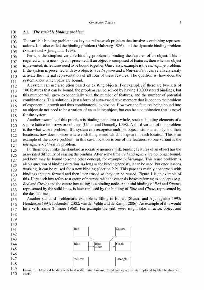
Furthermore, unlike the standard associative memory task, binding features of an object has theassociated difficulty of erasing the binding. After some time, red and square are no longer bound,and both may be bound to some other concept, for example red-triangle. This reuse problem isalso a question of binding duration. As long as the binding persists, it can be used, but once it stopsworking, it can be reused for a new binding (Section 2.2). This paper is mainly concerned withbindings that are formed and then later erased so they can be reused. Figure 1 is an example ofthis. Here each box refers to a group of neurons with the outer six boxes referring to concepts (e.g.Red and Circle) and the centre box acting as a binding node. An initial binding of Red and Square,represented by the solid lines, is later replaced by the binding of Blue and Circle, represented bythe dashed lines.

Another standard problematic example is filling in frames (Shastri and Aijanagadde 1993;Henderson 1994; Jackendoff 2002; van der Velde and de Kamps 2006). An example of this wouldbe a verb frame (Filmore 1968). For example the verb move might take an actor, object and

Red Square

Blue BindNode

Circle

Yellow Triangle

Figure 1. Idealised binding with bind node: initial binding of red and square is later replaced by blue binding withcircle.

151152153154155156157158159160161162163164165166167168169170171172173174175176177178179180181182183184185186187188189190191192193194195196197198199200

4 C.R. Huyck

location. In the sentence Pat moved the ball to the door. Pat would be the actor, the ball theobject, and to the door the location. When processing a sentence, the system would have tofill in the details by binding these objects to these slots. Perhaps frames are a common taskfor systems that use variable binding due to the compositional syntax and semantics prob-lems mentioned by early critics of connectionist systems (Fodor and Pylyshyn 1988). Framesare a flexible knowledge representation format (Schank and Abelson 1977); they are a rela-tional structure where data is used to fill in structures with variables. The basic frames aretemplates that need to be instantiated, and reused. Erasing the original’s filler is one mech-anism that can enable reuse. Moreover, if properly implemented, frames give compositionalsemantics.

Rules are another important case where variable binding is needed. Firstly, rule based systemsare Turing complete (Hopcroft and Ullman 1979), so a neural implementation of rules wouldbe Turing complete. This is not particular surprising as others have shown other connectionistsystems to be Turing complete (Siegelmann and Sontag 1991). Secondly, rules are widely usedas a means of modelling human cognition (Laird, Newell, and Rosenbloom 1987; Anderson andLebiere 1998), so rules are important for cognitive modelling. An example rule would be if Xgave Y to Z, then Z possesses Y. Finally, sequences are important and can be implemented byrules and by connectionist systems. For example, one system uses dynamic connections to learnsequences (Feldman 1982). These learned sequences are then automatically forgotten by a processof connection weight decay.

Unification is a more complex form of variable binding. This is done by symbolic systemssuch as language processing systems (Shieber 1986) and logic programming. There are a range ofunification approaches, and complex structures such as directed acyclic graphs may be com-bined (unified). It is a complex form of pattern matching. This can lead to a case where astructure may be illegally combined with a subset of itself, known as the occurs check (Browneand Sun 1999). Unification in neural systems may incorporate soft constraints making the sys-tem more flexible (Hofstadter 1979; Kaplan, Weaver, and French 1990). For instance, theremay be a grammar rule that combines a noun phrase and a verb phrase and requires that theyagree in number; a soft constraint may allow the same rule to apply, in some circumstances,when they do not agree in number, and this rule could be used to recognise ungrammaticalsentences.

A problem that is closely related to variable binding is Hetero-associative memory, which refersto the association of an input with an output. This is roughly what Smolensky (Smolensky 1990)refers to as variable binding, which differs from the term as used in this paper because hetero-associative memories are permanent or extremely long-lasting. Perhaps this difference is the basisof the term dynamic binding. To avoid confusion, in this paper, variable binding will only referto the case where a binding can be erased and reused.

Hetero-associative memory is a common and well understood form of memory (Willshaw,Buneman, and Longuet-Higgins 1969). Here items are combined, and each is linked to thatcombination. Presentation of one enables the system to retrieve the combined representation.Of course restrictions can be placed on the inputs, and several features may be needed toactivate the full set of items (Furber, Bainbridge, Cumpstey, and Temple 2004). Standard neu-ral models can account for this problem using standard Hebbian learning rules to implementa form of LTP (Gerstner and van Hemmen 1992) for permanent synaptic change. How-ever, this work is not easily extended to associative memories like semantic nets (Quillian1967). The problem here is that one memory needs to be associated with another, yet thetwo must remain separate. One excellent graph theoretic approach to this problem deals withbiological constraints on connectivity and activation (Valiant 2005). Both hetero-associativememory and associative memory, though related, are different from variable binding (but seeSection 6.3).

201202203204205206207208209210211212213214215216217218219220221222223224225226227228229230231232233234235236237238239240241242243244245246247248249250

Connection Science 5

2.2. Properties of binding mechanisms

Different binding mechanisms have different properties. This paper proposes that three propertiesare particularly important. These properties are:

(1) Persistence of binding(2) Number of bindings supported(3) Speed to bind

Others have discussed the number of bindings property (e.g. Shastri 2006; van der Velde andde Kamps 2006), but persistence of binding and speed to bind are not typically discussed. Thismay be due to other work on binding being almost exclusively based on bindings being supportedby neural firing (Section 6.2).

Persistence of binding has already been mentioned. Hetero-associative memories (Section 2.1),as typically modelled, persists forever. At the other extreme, binding via synchrony only persistsas long as at least one of the bound items is firing, and binding by active links persists as long asthe binding node is firing. This leaves a wide range of times that a binding might persist.

The number of bindings supported refers to how many entirely independent bindings, or distinctentities, can be supported simultaneously. One mechanism might be based on reusable bindingnodes. Each node might be used to support one binding, and there are as many bindings as nodes.Figure 1 has one binding node that can support any of the nine possible bindings of one colour andone shape. A second, or third, node could be added to support another. The solution of forminga dedicated binding node for each possible binding is impractical because it would require anexponential number of nodes, so the nodes must be reusable. Therefore, in the case of verb frames(Filmore 1968), each slot of each verb might be a binding node. The slot fillers could be simplenouns, or they could consist of other verbs, in for example the case of sentential complements, toallow an arbitrary degree of complexity. Of course complex noun phrases would also need bindingslots. With active links (van der Velde and de Kamps 2006) each binding node is represented bya circuit, and these can be combined to form verb frames. Binding via synchrony does not usenodes but has a limited number of bindings that a system can store (Sections 2.4.1 and 6.1).

Finally, time to bind is an important consideration. How long must items be coactive beforethey can be bound? Binding via synchrony is very fast and can occur within tens of ms (Wennekersand Palm 2000). The binding via LTP mechanism proposed below (Sections 3.1 and 4.2) takesmuch longer.

2.3. Cell assemblies and learning

A cell assembly (CA) is the neural basis of a symbol (Hebb 1949). A CA is a subset of neurons thathave high mutual synaptic strength enabling neurons in the CA to persistently fire after externalstimulation ceases. In the simulations discussed in this paper, a small subset of all the neuronsrepresents a symbol. If many of the neurons in the CA are firing, the symbol is active.

CAs give a sound answer to the neural representation of two types of memory, long-termmemory and short-term (or working) memory. The firing of many neurons in a CA is the neuralimplementation of short-term memory; this high frequency and persistent firing makes the CAactive.

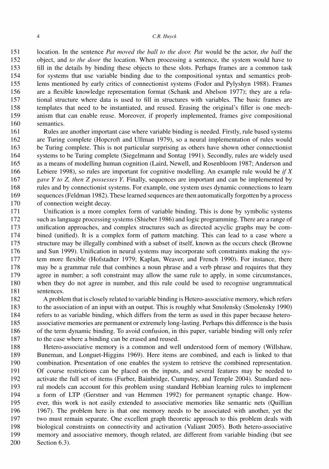
The red-square problem can be restated in terms of CAs. There is a CA each for red, blue,square, and circle. When a red-square and a blue-circle are presented, all four base CAs areactive. Figure 2 is an example of this problem. In this example, each cell represents a neuron withcircles representing neurons that fire in a given period. The relevant rows are labelled with allneurons in a row representing the appropriate feature, and CAs are represented by orthogonal sets

251252253254255256257258259260261262263264265266267268269270271272273274275276277278279280281282283284285286287288289290291292293294295296297298299300

6 C.R. Huyck

Square

Circle

Blue

Red

Figure 2. Sample neural firing pattern for red-square and blue-circle.

of neurons. In this case some, but not all, of the relevant neurons are firing. Somehow the pairsmust be bound, so that the system can ascertain, for example, the colour of the square, and thisbinding should only persist for a relatively small amount of time.

A CA is formed by a process of synaptic modification, and typically, this synaptic modi-fication is modelled as a form of LTP and long-term depression (LTD). CAs are long-termmemories with Hebbian learning rules providing the link between long- and short-term mem-ories (Hebb 1949; O’Neill, Senior, Allen, Huxter, and Csicsvari 2008). When neurons co-fire,they become more likely to fire together because their mutual synapses are strengthened (Hebb1949), and eventually, this can lead to the formation of a CA. Hebbian learning is local; itoccurs between two neurons that are connected and takes information based solely on theseneurons. Typically the synaptic weight is increased when both the pre-synaptic and post-synapticneurons fire. For all but the simplest forms of Hebbian learning, there is an associated formof forgetting that is, somewhat oddly, called anti-Hebbian learning. Here, if one neuron firesand the other does not, the synaptic weight is decreased (White, Levy, and Steward 1988),preventing the weight from growing without limit. There is significant biological evidence forHebbian learning (Miyashita 1988; Brunel 1996; Messinger, Squire, Zola, and Albright 2005).Moreover, as this learning is based on pairs of neurons, biological experiments are relativelysimple, so there is good reason to believe that some sort of Hebbian learning does occur inbrains.

None the less, the precise mechanisms that are used by biological systems are not entirelyclear. There are a range of Hebbian learning algorithms that follow the above definition, butdiffer from each other; none account for all biological data, and the biological data is far fromcomplete.

The simplest rule merely increases the synaptic weight when both neurons co-fire. There is noanti-Hebbian rule, and the weight may be clipped at some value (Sompolinsky 1987) to preventit growing without limit.

Timing is also important to learning. The Hebbian rule involves the firing of neurons at thesame time. In a model that uses continuous time, the same time requires some degree of flex-ibility. Work on Spike Timing Dependent Plasticity (Gerstner and Kistler 2002) adds anotherdimension to the complexity of Hebbian rules. In these rules, precise timing dynamics are impor-tant with the order of neural firing affecting whether the change in synaptic weight is positive ornegative.

The interaction between learning and firing leads to a complex dual dynamics (Hebb 1949).Once a CA is learned, it is hard to forget because any activation of it strengthens its intra-CAconnections; this is a form of the stability plasticity dilemma (Carpenter and Grossberg 1988; Fusi,Drew, and Abbott 2005). Similarly, it is difficult to do anything with a CA until it has formed.

Hebbian learning rules are the most widely accepted model of the mechanism used by thebrain to form CAs, the neural basis of concepts. Binding is not necessarily related to Hebbianlearning, but if CAs, once formed, can be appropriately bound, then the resulting system can havecompositional semantics and syntax. It then remains to ask what mechanisms can be used to bindCAs together?

301302303304305306307308309310311312313314315316317318319320321322323324325326327328329330331332333334335336337338339340341342343344345346347348349350

Connection Science 7

2.4. Solutions to the problem

The mechanism that is most commonly used in neural simulations of variable binding is synchrony(Malsburg 1981). A lesser used mechanism is active links (van der Velde and de Kamps 2006),and both require neural firing to maintain the binding.

2.4.1. Binding via synchrony

Binding via synchrony requires neurons that are bound together to fire together. Therefore, iftwo neurons are bound, they might fire at times X, X + 0.2, X + 0.5, X + 0.8, and X + 1. Forexample, the neurons might fire at 0.1, 0.3, 0.6, 0.9, and 1.1; and then repeat the pattern at 1.5,1.7, 2.0, 2.3, and 2.5. Of course there is some room for variation, and the binding usually appliesto a much larger number of neurons than two.

A good example of this is SHRUTI, a non-neural connectionist mechanism (Shastri andAijanagadde 1993). In this model, different sets of concept nodes are bound together by fir-ing at roughly the same time. Rules can be instantiated in the nodes, and these can continue topropagate the bindings to new items. SHRUTI has been used to develop, among other things, asyntactic parser (Henderson 1994). Here synchrony is used to bind slots and fillers. Unfortunately,the system only allows 10 bindings, so only relatively simple sentences can be processed.

There is significant evidence for synchronous firing in biological neural systems (Eckhornet al. 1988; Abeles, Bergman, Margalit, and Vaddia 1993; Bevan and Wilson 1999). Some reallyconvincing evidence that synchronous firing is used for biological binding is provided by a studythat shows how binding is facilitated by a stimulus that is presented synchronously (Usher andDonnelly 1998).

There are several simulated neural models of binding via synchrony (e.g. Bienenstock andMalsburg 1987; Wennekers and Palm 2000). Networks of spiking neurons are used to segmenta visual scene into different objects based on the firing timing of neurons associated with thoseobjects (Knoblauch and Palm 2001); a scene with a triangle and a square is presented, and neuronsassociated with the square fire together and the triangle neurons fire together, but at different timesfrom the square neurons. Spiking neurons are also used to parse simple text (Knoblauch, Markert,and Palm 2004) using binding via synchrony.

One major problem with binding via synchrony is the number of bindings that it supports(Section 2.2). The connectionist SHRUTI parser (Henderson 1994) is limited to 10 bindings, andShastri and Ajjanagadde suggest that this limit is about 10 (Shastri and Aijanagadde 1993). Allbound items must fire in roughly the same pattern, but to handle variations within neural behaviour,this pattern must be somewhat flexible. Similarly, items that are bound differently must fire in adifferent pattern. For example, the neurons in red and square must fire in roughly the same pattern,while the neurons in blue must fire in a pattern that is different from red. As these firing patternsmust occur in relatively brief time scales (∼33 ms), and they must be relatively flexible, thereare only a restricted number of bindings that can be maintained simultaneously. It is not entirelyclear how many bindings biological neural systems allow, but as more bindings exist, there is anincreased likelihood that closely related patterns will coalesce thus incorrectly combining sets ofbound items.

2.4.2. Binding via active links

A more recent approach to the binding problem creates active neural circuits to support the binding(van der Velde and de Kamps 2006). Both primitives and binding nodes are represented by neuralcircuits, similar to CAs. The binding is selected by active primitives and is maintained by neural

351352353354355356357358359360361362363364365366367368369370371372373374375376377378379380381382383384385386387388389390391392393394395396397398399400

8 C.R. Huyck

firing in the binding node. Like binding by synchrony, the binding stops once firing stops in thebinding node and stopping the binding circuit erases the binding. Binding can persist beyondfiring in the primitives.

Effective simulations of natural language processing and vision have been demonstrated. This isa promising mechanism for variable binding. The active neural circuit solution is similar to an olderconnectionist solution called dynamic connections (Feldman 1982). Dynamic connections areused to store bindings that are activated by a pair of inputs, and then persist for a considerableperiod. The persistence automatically decays allowing the node to be reused later.

2.4.3. Binding via LTP

Another option is to bind by changing synaptic weights. An earlier version of the work presentedin this paper used a fatiguing leaky integrate and fire (fLIF) neural model to implement rules tocount from one number to another (Huyck and Belavkin 2006). A Hebbian learning rule is usedto change synaptic weights permanently as a form of LTP.

Sougne provides an interesting blend between binding by changing synaptic weights and bind-ing by synchrony (Sougne 2001). The changing synapses regulate synchrony by modifying delayson connections.

Unfortunately, a general binding solution based on LTP faces the stability plasticity dilemma(Carpenter and Grossberg 1988). The dilemma is how is it possible to add new knowledge withoutdisrupting existing knowledge in a neural net (Lindsey 1988). With binding, base CAs would needto be stable, bindings would need to be plastic, and new CAs would still need to be formed. Thusany system that allowed a LTP based binding to be erased could have the problem of erasing thebase CAs that are being bound.

2.4.4. Other connectionist binding mechanisms

One standard mechanism is to create a new binding element for each possible binding. As men-tioned earlier (Section 2.1), this has the problem of combinatorial explosion. This combinatorialexplosion might be addressed by use of hierarchically allocated binding nodes (Hadley 2007)using prespecified roles. For natural language parsing, this requires millions of nodes, but thebrain has billions of neurons, so this is plausible.

Another connectionist mechanisms for binding is to merely combine the bound representations,but this leads to systems that have problems with compositional syntax. An example is TensorProduct binding (Smolensky 1990) which forms a type of cross product of the variables that arebeing bound.

While some work has been done on binding via synaptic change in neural systems, mostneural binding work has been done using synchronous firing. Some non-neural connectionistwork is relevant to the problem. However, the possibility of binding via synaptic change is anunder-explored area.

3. Binding via LTP and STP

There is strong evidence that distinct features that co-occur in a particular object cause synchronousneural firing (Eckhorn et al. 1988;Abeles et al. 1993; Usher and Donnelly 1998).While this appearsto be solid evidence for binding via synchrony, it is not conclusive proof. Synchronous firing maysimply be an emergent property of the neural representation of the new object as it is an emergentproperty of standard long-term CAs (Wennekers and Palm 2000). Assuming there is binding bysynchrony, it still has a problem with capacity and a problem with duration of binding.

401402403404405406407408409410411412413414415416417418419420421422423424425426427428429430431432433434435436437438439440441442443444445446447448449450

Connection Science 9

It is not entirely clear how many bindings can be maintained by a network at any given time,but each binding must have its own unique pattern of synchrony (Section 2.4.1). Natural languageprocessing may require many bindings as do other tasks such as object recognition. Since CAscross brain areas (Pulvermuller 1999), orthogonalising domains (e.g. vision and language) is nota viable solution; that is, the brain can not be partitioned into areas where bindings are distinct sothat binding frequencies can simultaneously support multiple distinct bindings.

Also, the synchronous binding only persists as long as the CAs are active. Once they stop, thebinding is lost. While it is not entirely clear how long memories persist, there is a wide range oftimes over which a binding might persist.

Even if binding via synchrony occurs in the brain, this does not mean that there are not othertypes of binding. A different mechanism for binding, as is shown below, is change in synapticweights. There are at least two variants of known biological synaptic weight change, LTP and STP.

3.1. Binding via LTP

One possible solution to the binding problem is permanent synaptic change; biologically this isLTP and LTD. Objects are bound using synaptic weight change, and these weight changes remainuntil future learning erases them.

For LTP to be able to solve the variable binding problem, the binding must be able to be erased.The mechanism then faces the stability plasticity dilemma (Carpenter and Grossberg 1988). If thesame mechanism is used to form the initial memories and to do the binding, something else mustprevent the initial memories from being erased when the bindings are erased.

3.2. Binding via STP

Most simulation work that involves learning relies on LTP. However there is another type of learn-ing, STP, and there is extensive evidence that STP occurs in biological neural systems (Buonomano1999; Hempel, Hartman, Wang, Turrigiano, and Nelson 2000). It is still a type of Hebbian learn-ing, based on the firing behaviour of the neurons a synapse connects, so that co-firing increasesthe synaptic weight. However, unlike LTP, the change is not permanent.

Some have proposed that STP provides support for LTP (Kaplan, Sontag, and Chown 1991).That is, in the initial stage of CA formation, short-term connection strength adds activation to thenascent CA that supports the co-firing that provides impetus for LTP. More recently, short-termconnection strength has been proposed as another basis of working memory (Fusi 2008; Mongillo,Barak, and Tsodyks 2008). This contradicts the basic idea of active CAs as the basis of workingmemory, but the two proposals may be compatible.

Another use for STP is for binding. In this case, the base memories are bound using STP. Asthe STP is automatically erased, so is the associated binding. This paper is the first to describethe use of STP in simulations of binding.

Note that the four binding mechanisms, synchrony, active links, compensatory LTP and STP,are not mutually exclusive. Section 5.4 shows synchronous firing behaviour alongside bindingvia LTP and STP, and describes how all four mechanisms could be combined in a single system.

4. Simulating binding with LTP and STP

To show that the STP and compensatory LTP binding mechanisms function, simulations of asimple paired association task, similar to the red-square problem (Section 2.1), are described.These and all the simulations described in this paper, use the same basic fLIF neural model.

451452453454455456457458459460461462463464465466467468469470471472473474475476477478479480481482483484485486487488489490491492493494495496497498499500

10 C.R. Huyck

4.1. fLIF model

The neural model that is used for the simulations described in this paper is an extension of thestandard leaky integrate and fire (LIF) model which is in turn an extension of the integrate and fire(IF) model. A similar model (Chacron, Pakdaman, and Longtin 2003) has been shown to accountfor inter-spike intervals under various input conditions better than the standard LIF model. TheIF model, commonly called the McCulloch Pitts neuron (McCulloch and Pitts 1943), has a longstanding history and is quite simple. Roughly, neurons are connected by uni-directional synapses.A neuron integrates activity from the synapses connected to it, and if the activity surpasses athreshold, the neuron fires sending activity to the neurons it connects to. Connections may beexcitatory or inhibitory; excitatory connections adding activity from the post-synaptic neuron andinhibitory connections subtract activity. LIF models are more biologically faithful than simple IFmodels (Churchland and Sejnowski 1992). In the IF model, if a neuron does not fire, it loses allits activity. In the LIF model, a neuron retains a portion of that activity making it easier to firelater. Typically, the neuron loses all its activity when it fires (Maass and Bishop 2001). All of thesemodels are less complex and less accurate than Hodgkin Huxley models (Hodgkin and Huxley1952) and other compartmental models (Dayan and Abbott 2005) which are extremely faithfulto biology, breaking each neuron into several compartments and modelling interactions on a finetime grain (<1 ms).

The simulator runs in discrete steps with every neuron being modified in each step, and activitybeing collected in the next. The network of neurons can be broken into a series of subnets. Eachneuron has two variables associated with it, and an array of synapses, and each subnet has fourconstants associated with all its neurons.

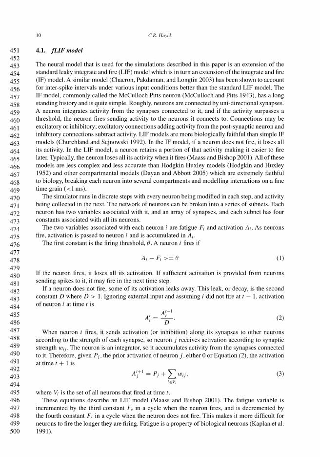
The two variables associated with each neuron i are fatigue Fi and activation Ai . As neuronsfire, activation is passed to neuron i and is accumulated in Ai .

The first constant is the firing threshold, θ . A neuron i fires if

Ai − Fi >= θ (1)

If the neuron fires, it loses all its activation. If sufficient activation is provided from neuronssending spikes to it, it may fire in the next time step.

If a neuron does not fire, some of its activation leaks away. This leak, or decay, is the secondconstant D where D > 1. Ignoring external input and assuming i did not fire at t − 1, activationof neuron i at time t is

Ati = At−1

i

D. (2)

When neuron i fires, it sends activation (or inhibition) along its synapses to other neuronsaccording to the strength of each synapse, so neuron j receives activation according to synapticstrength wij . The neuron is an integrator, so it accumulates activity from the synapses connectedto it. Therefore, given Pj , the prior activation of neuron j , either 0 or Equation (2), the activationat time t + 1 is

At+1j = Pj +

∑

i∈Vi

wij , (3)

where Vi is the set of all neurons that fired at time t .These equations describe an LIF model (Maass and Bishop 2001). The fatigue variable is

incremented by the third constant Fc in a cycle when the neuron fires, and is decremented bythe fourth constant Fr in a cycle when the neuron does not fire. This makes it more difficult forneurons to fire the longer they are firing. Fatigue is a property of biological neurons (Kaplan et al.1991).

501502503504505506507508509510511512513514515516517518519520521522523524525526527528529530531532533534535536537538539540541542543544545546547548549550

Connection Science 11

The model has a loose link with time in biological neurons. The model does not incorporateconductance delays or refractory periods, and these behaviours all happen in under 10 ms, soeach given cycle can be considered to be roughly 10 ms. Consequently, each neuron emits atmost one spike per 10 ms. of simulated time, and the timing precision is at most 10 ms. This is ashortcoming of the model, but enables efficient simulation of hundreds of thousands of neuronson a standard PC.

The model also has some degree of topological faithfulness. The Hopfield Net (Hopfield 1982)has been a popular system for modelling brain function (Amit 1989), but it requires neurons to bewell connected and connections to be bi-directional. Neither constraint is biologically accurate.However, one key point that these and other attractor nets (e.g. Rumelhart and McClelland 1982;Ackley, Hinton, and Sejnowski 1985) show is that attractor states are important; an attractor stateis where roughly the same neurons and only those neurons fire in each cycle. This is a key pointof CAs (Section 2.3).

The system uses neurons that are either inhibitory or excitatory but not both. While there issome debate over the biological behaviour, this follows the strict constraint of Dale’s Law (Eccles1986). In the simulations described in this section, the ratio is 4 excitatory to 1 inhibitory neuronas is claimed in the mammalian cortex (Braitenberg 1989).

The connectivity of the network, and subnets is also important. Like the mammalian brain,excitatory neurons are likely to connect to neurons that are nearby. The network is broken intoa series of rectangular subnets. As distance is relevant, the topology of each subnet is toroidal(the top is adjacent to the bottom, and sides are adjacent to each other, like folding a piece ofpaper into a donut) to avoid edge problems. In the simulations described in this section, excitatoryneurons also have one long distance axon with several synapses. So a neuron connects to nearbyneurons and to neurons in one other area of the subnet. These connections are assigned randomly,so each new subnet is extremely unlikely to have the same topology as another subnet with thesame number of neurons. Equation (4) is used for connectivity.

r <1

(N ∗ 8)−→ connect. (4)

It is initially called for each neuron with N (distance) of one for three adjacent neurons. It issubsequently called recursively on all four adjacent neurons with distance increasing one on eachrecursive call, and the recursion is stopped at distance 5. r is a random number between 0 and 1.The long-distance axon uses the same process though starts with distance 2. Inhibitory neuronsare connected randomly within a subnet. This makes it easier for localised CAs to inhibit eachother. There are approximately 60 synapses leaving a neuron to other neurons in the subnet, forboth inhibitory and excitatory neurons.

4.2. Simulating binding by compensatory LTP

The first set of simulations being reported in this paper involve binding via permanent changes ofsynaptic strength. This involves a compensatory Hebbian learning mechanism (Huyck 2004) thatmakes permanent changes to increase a synapse’s strength, akin to LTP, and permanent changesthat decrease the strength, akin to LTD. The simulation also makes use of spontaneous neuralactivation, a known biological phenomenon (Amit and Brunel 1997), to support erasing bindings.

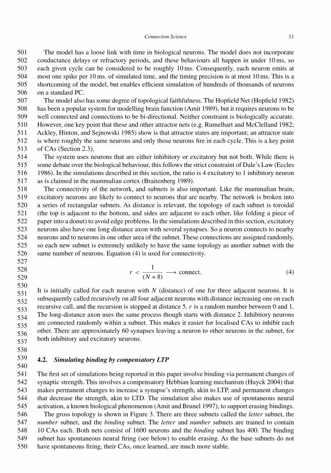
The gross topology is shown in Figure 3. There are three subnets called the letter subnet, thenumber subnet, and the binding subnet. The letter and number subnets are trained to contain10 CAs each. Both nets consist of 1600 neurons and the binding subnet has 400. The bindingsubnet has spontaneous neural firing (see below) to enable erasing. As the base subnets do nothave spontaneous firing, their CAs, once learned, are much more stable.

551552553554555556557558559560561562563564565566567568569570571572573574575576577578579580581582583584585586587588589590591592593594595596597598599600

12 C.R. Huyck

NumberSubnet

LetterSubnet

BindSubnet

Figure 3. Topology of intra-subnet connections in the compensatory LTP binding simulation: each neuron in the basesubnets connect to the bind subnet, and each neuron in the bind subnet connects to the base subnets.

In addition to the intra-subnet connection, each bind neuron has 15 connections to both theother subnets. The neurons of the base subnets, letter and number, have 16 connections to thebind subnet and all inter-subnetwork connections are randomly assigned. The initial weights areinitialised to a number close to 0.

The compensatory learning mechanism is another type of Hebbian learning. It forces the totalsynaptic strength leaving a neuron towards the desired weight, WB . Elsewhere (Huyck 2007),this learning mechanism has been used to learn hierarchical categories where categories shareneurons. Compensatory learning is biologically plausible because the overall activation a neuroncan emit is limited. Since a neuron is a biological cell, it has limited resources, and synapticstrength may well be one such resource.

The compensatory rule modifies the correlatory learning rules to include a goal total synapticweight WB . Equation (5) is the compensatory increase rule and Equation (6) is the compensatorydecreasing rule; that is, Equation (5) is a Hebbian rule and Equation (6) an anti-Hebbian rule. WB

is a constant which represents the desired total synaptic strength of the pre-synaptic neuron, andWi is the current total synaptic strength. R is the learning rate, which is 0.1. P is a constant andmust be greater than 1. The larger it is, the less variance the total synaptic weight has from WB . P ,WB , and R are constants associated with a particular subnet. When the two neurons co-fire thereis an increase in synaptic weight corresponding to Equation (5). If the pre-synaptic neuron firesand the post-synaptic neuron does not fire, the weight is decreased according to Equation (6).

�+wij = (1 − wij ) ∗ R ∗ P (WB−Wi), (5)

�−wij = wij ∗ −R ∗ P (Wi−WB). (6)

Compensatory learning is important in the erasing process described below.A summary of the value of the constants used in the first simulation can be found inTable 1.These

values were determined by exploration of the parameter space via simulation. The parameter space,including topology, is practically infinite. This particular location is almost certainly not optimal,but does show solid results. An understanding of the dynamics of CA activation and formationis essential to select these parameters; this includes knowledge of various tradeoffs betweenparameters such as reducing firing threshold is similar to increasing synaptic strength. To a lesserextent, biological constraints also help in directing the search. For instance, excitatory synapticweight is in the range of 0–1, and it is known that several neurons are needed to cause another

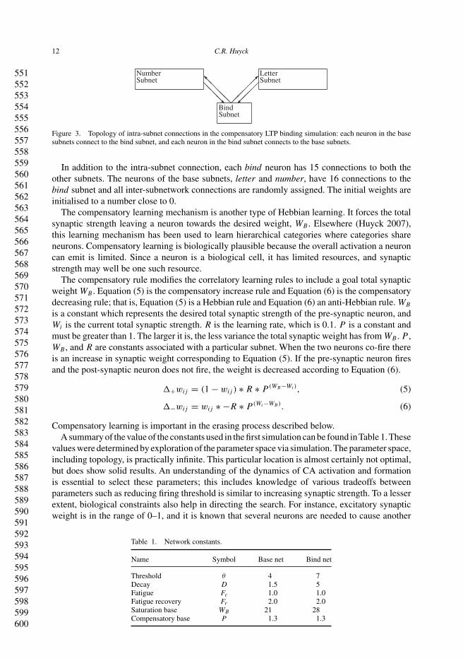
Table 1. Network constants.

Name Symbol Base net Bind net

Threshold θ 4 7Decay D 1.5 5Fatigue Fc 1.0 1.0Fatigue recovery Fr 2.0 2.0Saturation base WB 21 28Compensatory base P 1.3 1.3

601602603604605606607608609610611612613614615616617618619620621622623624625626627628629630631632633634635636637638639640641642643644645646647648649650

Connection Science 13

to fire (Abeles 1991) so the threshold θ is much greater than that. In one study of anaesthetisedguinea pigs, simulated models accounted for spiking behaviour when decay was roughly D = 1.25(Lansky, Sanda, and He 2006).

During the entire run, there is spontaneous activation in the binding net. Spontaneous neuralfiring is a property of biological neurons (Abeles et al. 1993; Amit and Brunel 1997; Bevan andWilson 1999), and it has been proposed as a mechanism for weakening and even erasing memories(Huyck and Bowles 2004).

In this simulation, some neurons may be spontaneously activated. This is modelled by theselection of a random number 0 ≤ r < 1 for each neuron in each cycle. If the r < 0.03 the neuronis spontaneously active. Therefore, roughly 3% of neurons in the bind subnet fire spontaneouslyeach cycle.

The simulation first learns the base number and letter CAs, then one of each is randomlyselected to be bound. This is a simple paired association task similar to the task performed inearlier connectionist simulations (Feldman 1982) and those done in psychological experiments(e.g. Sakai and Miyashita 1991). Once bound, the binding is tested, followed by a test for anunbound letter and number. The binding is then erased by spontaneous activation; and the testsare rerun. For measurement, this binding, testing, erasing, and retesting process is repeated 10times on each of 10 different networks.

The base CAs are learned by merely presenting components of them. As both the base netsconsist of 1600 neurons, they can be divided into 10 orthogonal CAs of 160 neurons each. Fiftyrandomly selected neurons of a particular CA are selected and presented for 10 cycles. This isakin to clamping, but these neurons are given θ ∗ (1 + random) units of activation. After fatiguehas accumulated they may not fire. After the 10 cycles of activation, the network is allowed torun for 40 more cycles. It is then reset with all activation and fatigue zeroed. Then a new CA ispresented. Each set of 50 cycles of activation, run-on, and short-term variable resetting is calledan epoch.

Each base CA is presented in a rotation so that all CAs are presented once every 1000 cycles.The complete training phase is 20,000 cycles so that each base CA is presented 20 times. Notethat spontaneous activation in the bind net continues throughout this time.

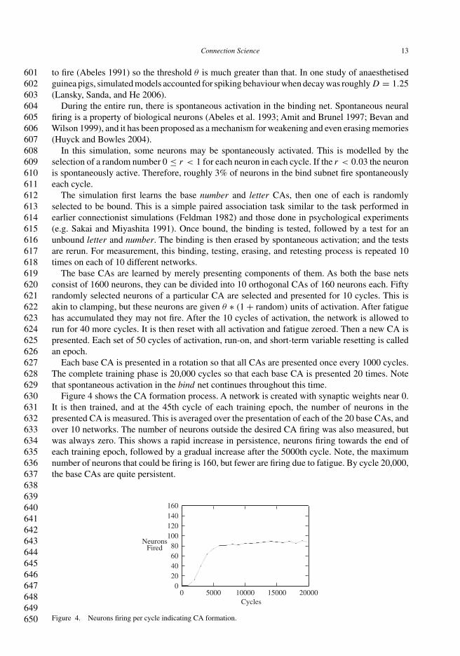
Figure 4 shows the CA formation process. A network is created with synaptic weights near 0.It is then trained, and at the 45th cycle of each training epoch, the number of neurons in thepresented CA is measured. This is averaged over the presentation of each of the 20 base CAs, andover 10 networks. The number of neurons outside the desired CA firing was also measured, butwas always zero. This shows a rapid increase in persistence, neurons firing towards the end ofeach training epoch, followed by a gradual increase after the 5000th cycle. Note, the maximumnumber of neurons that could be firing is 160, but fewer are firing due to fatigue. By cycle 20,000,the base CAs are quite persistent.

020406080

100120140160

0 5000 10000 15000 20000

NeuronsFired

Cycles

Figure 4. Neurons firing per cycle indicating CA formation.

651652653654655656657658659660661662663664665666667668669670671672673674675676677678679680681682683684685686687688689690691692693694695696697698699700

14 C.R. Huyck

After the training phase, the epoch duration is lengthened to 1000 cycles for the binding phase.Arandomly selected letter CA and a randomly selected number CA are presented simultaneously.In a system that accepted visual input, both items would be presented simultaneously as in apaired association task. In this simulation, 50 neurons from both CAs are selected at randomand presented for 10 cycles. As the CAs are already formed, these almost always persist for theduration of the binding epoch.

As ever, the bind subnet is spontaneously activated during this phase. Throughout this periodthe synaptic weights between the subnets gradually increase. When binding is successful, neuronsin the bind subnet fire due to input from the active number and letter CA. This in turn causes theinter-subnet synapses to increase. In essence, a new CA is being formed and it includes neuronsfrom all three subnetworks.

It is crucial that two CAs in the base subnets are simultaneously active. This is similar to themechanism used for node activation by dynamic connections (Feldman 1982). Along with thespontaneously active bind neurons, these base neurons provide sufficient activation to fire someof the neurons in the bind subnet. Firing these base neurons causes the mutual synaptic strengthbetween them and the base neurons to increase leading to further neural firing in the bind subnet.By the end of the binding epoch, a CA has been formed that includes the binding neurons, andthis composite CA can be reactivated at any time over a significant period of time.

In the second epoch, the bound number is presented, and in the third, the bound letter ispresented. When successful, this leads to activation of the binding CA and the opposite base CA.This further reinforces the inter-subnet synaptic strengths, improving the binding.

In the fourth epoch a randomly selected unbound number is presented, and an unbound letteris presented in the fifth. The correct result here is that no neurons in the opposite subnetwork fire.

The synaptic strength from the binding subnet that supports the binding is being reduced duringthe test unbound phase, but four further epochs of no base presentation are run to allow the bindingto be sufficiently erased. The synapses from the binding subnet that support the binding moverapidly towards zero due to the application of compensatory learning rules (Equations (5) and(6)) caused by spontaneous firing.

Synapses from the bind subnet to the base subnets are erased during the period of no presenta-tion. During this period, neurons in the bind subnet fire, but no neurons in the base subnets fire.Consequently, the weights are reduced towards 0.

However, the synapses to the bind subnet from the base subnets are not changed during thetesting of unbound items or during the period of no presentation. Instead, these synapses arereduced by the compensatory learning mechanism during the next two test epochs (epochs sevenand eight).

The synaptic weights from neurons in the base subnets to the bind subnet do not change betweenthe last binding test, and the first bind retest. Why then does the presentation of the here to forebound item not cause the bind subnet to activate as it had done during the presentation in thesecond and third epochs?

Firstly, there are fewer neurons firing in the just bound item. This is due to the loss of intra-subnet synaptic strength during the binding. Secondly, there is little initial feedback from the bindnode since its neurons no longer have much synaptic weight to the recently bound item. Duringthis initial phase, the synaptic weights in the just bound item are changing. The weights to thebind node are being reduced while the weights within the just bound item are increasing. Thereis only a small part of the parameter space where this difficult task can be solved (Section 4.4).

Finally, there are four tests to assure that the binding has been erased. The formerly boundnumber and letter CAs are presented, followed by the formerly tested unbound number and letter.

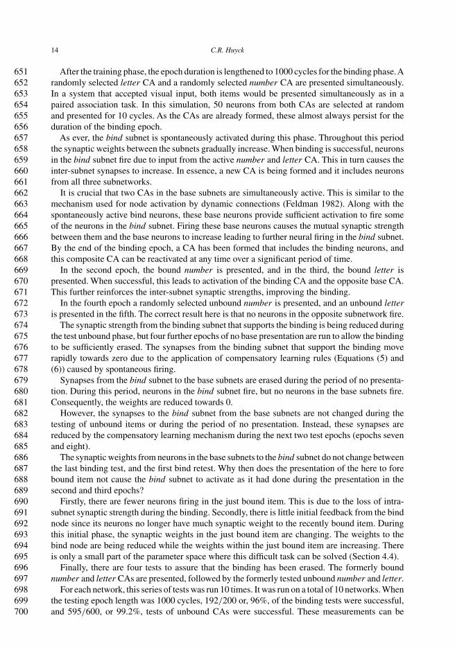
For each network, this series of tests was run 10 times. It was run on a total of 10 networks. Whenthe testing epoch length was 1000 cycles, 192/200 or, 96%, of the binding tests were successful,and 595/600, or 99.2%, tests of unbound CAs were successful. These measurements can be

701702703704705706707708709710711712713714715716717718719720721722723724725726727728729730731732733734735736737738739740741742743744745746747748749750

Connection Science 15

combined using a standard F-2 (2 ∗ Bound ∗ Unbound)/(Bound + Unbound). The F-score is97.5%.

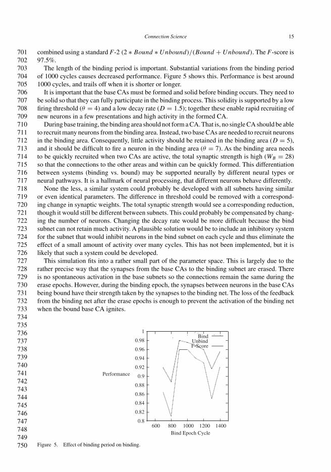
The length of the binding period is important. Substantial variations from the binding periodof 1000 cycles causes decreased performance. Figure 5 shows this. Performance is best around1000 cycles, and trails off when it is shorter or longer.

It is important that the base CAs must be formed and solid before binding occurs. They need tobe solid so that they can fully participate in the binding process. This solidity is supported by a lowfiring threshold (θ = 4) and a low decay rate (D = 1.5); together these enable rapid recruiting ofnew neurons in a few presentations and high activity in the formed CA.

During base training, the binding area should not form a CA. That is, no single CA should be ableto recruit many neurons from the binding area. Instead, two base CAs are needed to recruit neuronsin the binding area. Consequently, little activity should be retained in the binding area (D = 5),and it should be difficult to fire a neuron in the binding area (θ = 7). As the binding area needsto be quickly recruited when two CAs are active, the total synaptic strength is high (WB = 28)so that the connections to the other areas and within can be quickly formed. This differentiationbetween systems (binding vs. bound) may be supported neurally by different neural types orneural pathways. It is a hallmark of neural processing, that different neurons behave differently.

None the less, a similar system could probably be developed with all subnets having similaror even identical parameters. The difference in threshold could be removed with a correspond-ing change in synaptic weights. The total synaptic strength would see a corresponding reduction,though it would still be different between subnets. This could probably be compensated by chang-ing the number of neurons. Changing the decay rate would be more difficult because the bindsubnet can not retain much activity. A plausible solution would be to include an inhibitory systemfor the subnet that would inhibit neurons in the bind subnet on each cycle and thus eliminate theeffect of a small amount of activity over many cycles. This has not been implemented, but it islikely that such a system could be developed.

This simulation fits into a rather small part of the parameter space. This is largely due to therather precise way that the synapses from the base CAs to the binding subnet are erased. Thereis no spontaneous activation in the base subnets so the connections remain the same during theerase epochs. However, during the binding epoch, the synapses between neurons in the base CAsbeing bound have their strength taken by the synapses to the binding net. The loss of the feedbackfrom the binding net after the erase epochs is enough to prevent the activation of the binding netwhen the bound base CA ignites.

0.8

0.82

0.84

0.86

0.88

0.9

0.92

0.94

0.96

0.98

1

600 800 1000 1200 1400

Performance

Bind Epoch Cycle

BindUnbindF-Score

Figure 5. Effect of binding period on binding.

751752753754755756757758759760761762763764765766767768769770771772773774775776777778779780781782783784785786787788789790791792793794795796797798799800

16 C.R. Huyck

Since this is so precise, minor changes to parameters cause a rapid decrease in performance.Changing the number of synapses from each base neuron to the bind neurons from 16 to 15 givesBound/Unbound/F-Score results of 87%/95.5%/91.1%, and changing the number from 16 to17 gives B/U/F results of 78.5%/94.8%/85.9%. Similarly, changing the base nets’ desired totalsynaptic strength (WB) from 21 to 20 gives B/U/F results of 45%/99.2%/61.9%, and changing itfrom 21 to 22 gives results of 80.5%/89.8%/84.9%. Changing parameters individually is a formof gradient descent search; while gradient descent is not the best way to find an optimal place inthe space, it can help to find local minima.

This is a particularly difficult binding simulation because there is no spontaneous activation inthe base nets to facilitate erasing the binding. However, the lack of this spontaneous activationallows those CAs to persist indefinitely. Additionally, binding still works quite effectively.

4.3. Simulating binding by STP

Another option to implement variable binding by synaptic modification is to change the basicmechanism of synaptic change. LTP and LTD require the synaptic weight to remain unchangeduntil there is another application of one of the rules. Since synaptic change is caused by neuralfiring, the synaptic weights will remain unchanged until the appropriate neurons fire.

Another option is to have the weights automatically revert to zero over time. A rule that did thiswould be akin to STP. Note that the rule is still Hebbian in nature, changing the synaptic weightbased solely on the firing behaviour of the two neurons that a synapse connects, but in this case,the weight also changes towards 0 when there is no firing.

The binding via STP simulations reported below are identical to the binding via compensatoryLTP simulations (Section 4.2) except the bind subnet is removed, neurons are replaced by neuronsthat learn via both LTP and STP, and the binding epochs are 50 cycles. The bind subnet wasprovided to localise erasing of bindings; with STP the bindings are automatically erased at theneural level.

For STP, the simulation uses a new type of model neuron, termed a fast-bind neuron. The basicproperties remain the same (Section 4.1), but some of the synapses leaving these neurons changetheir weights based on a different mechanism that accounts for STP.

The learning rule for fast-bind synapses that was used in these simulations is the simplest typeof Hebbian learning. For each fast-bind synapse, if the pre-synaptic neuron fires in the same cycleas the post-synaptic neuron, the strength increases by the learning constant, which is 0.1. Theweight is clipped at 1.

The rule for reducing synaptic weight is equally simple. If the neuron does not fire in a cycle, allfast-bind synapses leaving it have their weight decreased by a constant k (in this case k = 0.004which was selected to assure the binding persisted for roughly 250 cycles after last use). Therefore,a maximally weighted synapse, will return to 0 after 250 cycles of inactivity. Similarly, a minimallyweighted synapse will go to 1 after 10 cycles of pre and post-synaptic co-firing.

The topology of the number and letter subnets is the same as in the LTP simulations, with 80%excitatory and 20% inhibitory, and inhibitory neurons have no fast-bind synapses. Each neuronhas two fast-bind synapses to neurons in each CA in the opposite subnet, and those neurons arerandomly selected.

The constants of the letter and number nets are the same as those in the LTP experiment; theseare shown in Table 1. The training length is the same, 20,000 cycles, and the procedure is thesame. The testing patterns are the same: binding epoch, two bind test epochs, two unbound testepochs, four epochs with no presentation, then two more tests of the formerly bound CAs, andtwo tests of the unbound CAs.

When the epoch lengths are 50 cycles, the system performs perfectly over 10 bindings on each of10 nets. That is, all 100 bindings were successful, and all associated 100 erasings were successful.

801802803804805806807808809810811812813814815816817818819820821822823824825826827828829830831832833834835836837838839840841842843844845846847848849850

Connection Science 17

The Bound/Unbound/F-Score results are 100%/100%/100%. The bindings only need 10 cyclesto be fully established, and as they are given 50, they are firmly established. Similarly, only 250cycles are needed for the bindings to be fully erased. As there are two unbound test epochs, andfour non-presentation epochs after the binding, there are 300 cycles of erasing, so erasing is alsoperfect.

4.4. Performance of LTP vs. STP

It has been significantly simpler to use binding by STP than to use binding by compensatory LTP.The portion of the parameter space that has been explored, where binding via compensatory LTPfunctions acceptably, is quite small. This has required the use of relatively precise topologies,precise training and use regimes, and spontaneous activation has been used only in the Bindsubnet to support erasing. On the other hand, binding by STP works in a much larger range ofconditions, and no exploration was done as the parameters for the LTP experiment were used.The manipulation of learning and forgetting weights allows for a corresponding manipulation ofbind and unbind times (Section 5.2). Consequently, the next section discusses simulations usingbinding by STP to account for crosstalk and compositionality.

Compensatory LTP should be able to account for these phenomena, but complex trainingregimes may be needed, so at this juncture it seems unwise to describe further LTP simulations.The basic problem with binding by compensatory LTP along with erasing by spontaneous acti-vation is that it faces the stability plasticity dilemma. Some memories are stable, the items beingbound, and some are not, the bindings. It is difficult for the same mechanism to account for both.Formation of bindings is slow and they persist for a long time, just like CAs, so it may be betterto view binding by compensatory LTP as a form of associative memory. However, this provides anew way of addressing the stability plasticity dilemma that is more fully discussed in Section 6.3.

The above simulations use fLIF neurons, but binding by compensatory LTP and STP shouldboth be applicable to other neural systems. Spiking models are particularly appropriate (e.g. Maassand Bishop 2001). The rules may force breaking of the constraints of some attractor nets (e.g.Hopfield Net connections would no longer be bidirectional), but this is not incompatible from asimulation perspective (Amit 1989). Continuous value output neural models (e.g. Rumelhart andMcClelland 1982) should also be compatible with binding via STP. It is not entirely clear howspontaneous activation would be implemented in these models, but compensatory learning shouldstill work. It is also not clear how these mechanisms would apply to connectionist systems that donot have a close relationship to biological neurons like multi-layer perceptrons (Rumelhart andMcClelland 1986).

The binding by compensatory LTP and binding by STP models that are presented in this paperare examples of classes of learning algorithms. The compensatory LTP mechanism was chosenbecause a compensatory mechanism eases recruitment of new neurons to a CA, binding, andsupports erasing. The STP mechanism was chosen because of its simplicity. Ultimately, it ishoped that the neurobiological basis of neural learning will be sufficiently illuminated to saywhich algorithms are used for memory formation and variable binding in the biological system.Until then, an exploration of different binding algorithms and their use in large systems to simulatecomplex behaviour may be a good way to explore alternative neural binding mechanisms.

5. Further evaluation of binding by STP

In the binding by compensatory LTP simulation (Section 4.2), a binding node was used. In theSTP simulation (Section 4.3) no explicit binding node was used, but implicitly, each CA was a

851852853854855856857858859860861862863864865866867868869870871872873874875876877878879880881882883884885886887888889890891892893894895896897898899900

18 C.R. Huyck

binding node so that 20 bindings could be supported. This required that each CA was connectedto each CA in the opposite subnet, and this would require a geometric growth in synapses as thenumber of base CAs grew linearly. The use of binding nodes can make growth of synapses growlinearly as the base CAs grow linearly with each base CA connecting to the binding node. Ofcourse, it is also possible to have many binding nodes to support multiple bindings at a giventime. How do multiple bindings interact and how many can be supported?

5.1. Crosstalk

In this section, a system that stores multiple bindings is described. Storing these bindings couldlead to problems of cross talk, but none are seen. The simulation combines both STP and LTP ona single neuron with specific synapses devoted to each. The gross topology is similar to that ofFigure 3, but in this experiment there are multiple binding nodes.

There are four CAs in the letter subnet, four in number and four in bind. The letter and numberCAs consist of 160 neurons each and the bind CAs have 100.All excitatory neurons have synapsesleaving them that are modified by the compensatory LTP rule and synapses that are modified by theSTP rule. The intra-subnet connections are the same as in the experiment described in Section 4.2and all of these are modified by compensatory LTP.

Each neuron also has connections outside of the subnet and these are governed by the STP rule.Each neuron in the letter and number subnets has two connections to a randomly selected neuronin each CA in the bind subnet, and each of the bind neurons had three connections to each CAin the other subnets. This means that each neuron received roughly the same number of fast bindinputs as those in Section 4.3.

As in Sections 4.2 and 4.3, the base CAs were trained for 20 epochs of 50 cycles each. Thisformed stable CAs, and there was no spontaneous activation. The constants were the same as thosefor the base subnets in Table 1 (θ = 4, D = 1.5, Fc = 1.0, Fr = 2.0,WB = 21, and P = 1.3).

Bindings were set by a single epoch of 50 cycles of presentation of one letter, one bind, andone number CA. Initially this was A0, B1, C2, and D3 each with a unique binding node.

Testing followed immediately with the numbers being presented in order. At the end of 50cycles, the net was reset and the next number presented. On 100 nets, 400 of 400 correct bind andletter CAs fired in cycle 49 and no other neurons in those subnets fired. As expected, a randomone to one binding (e.g. A1, B2, C3, D0 each with a unique binding node) faired as well.

This test means that bindings are set and then allowed to be maintained without activation for150 cycles. With automatic synaptic reduction set at 0.004 (k = 0.004) for each cycle when thepre-synaptic neuron does not fire, the synaptic weights return to zero after 250 cycles of inactivity.The simulation is run with a 50 cycle rest after the last binding, for a total of 200 cycles betweenthe last cycle of each binding and each test. On 100 nets, none of the letter CAs have neuronsfiring, though 21 of the 400 bind nodes have some firing. The simulation was run with a 100 cyclerest after the bindings are set, and indeed the weights have returned to 0 and no firing was foundin the bind and letter subnets.

The bindings are not formed simultaneously. So simultaneous presentation of red-square andblue-circle to the visual channel could not readily form two separate bindings. An attentionalmechanism might be used with one object being attended to first and bound, followed by thesecond. Alternately, a different mechanism, e.g. active links, could be used to solve this problem(Section 5.4).

One common problem with binding is the presentation of two overlapping bindings, e.g. ared-triangle, and a red-square. This has been called the problem of two (Jackendoff 2002). Thishas been solved by a separate binding node for each pair (van der Velde and de Kamps 2006);elsewhere, this binding has been modelled with a computer simulation of CAs (deVries 2004) toaccount for psychological evidence.

901902903904905906907908909910911912913914915916917918919920921922923924925926927928929930931932933934935936937938939940941942943944945946947948949950

Connection Science 19

The simulation was modified so that A0, B1, C0, and D1 were presented, each with a uniquebinding node. When the letter was presented the correct number CA was highly active with noincorrect neurons firing for each of the 400 presentations on 100 tests. This shows that the bindingby STP addresses the problem of two.

Another test was done by presenting the number. When 0 was presented either A, C, or bothcould ignite; and B, D, or both could ignite for 1. On 100 runs, when 2 or 3 were presented, noletter neuron fired. Of the 200 positive tests, both of the bound letter CAs had over 100 neuronsfire 158 times, between 10 and 100 fired in one and the other was over 100 21 times, and in 21tests fewer than 10 neurons fired in one while the other was near peak. This means that usuallyboth of the bound CAs ignited, but occasionally, due to competition, only one did.

As described in Section 4.1, each subnet is set up as a competitive subnetwork, with inhibitoryneurons that connect randomly within the subnet. In this case, each inhibitory neuron had 60synapses. Fewer synapses lead to less competition, and more synapses to more competition. With30 synapses on one hundred runs, both letter CAs fired on each of the 200 tests, though on twotests less than 100 neurons fired in one CA. With 90 synapses on 100 runs on all 200 tests onlyone was active and the other had less than ten neurons firing. Note that an inappropriate neuronwas never seen firing. Therefore, with ambiguous bindings, behaviour is dependent on the extentof competition.

5.2. Capacity

In some sense, an exploration of the number of bindings that can be simultaneously supportedby STP is unnecessary. It is obvious that different orthogonal bindings can be independentlysupported. For instance, filling in the topology for Figure 1 with values from the simulationsof Section 5.1 means that each orthogonal binding set can be represented by six base CAs of160 neurons, and one binding CA of 100 neurons, or 1060 neurons. Therefore, the brain has acapacity for billions of these orthogonal bindings, though it is extremely doubtful that the brainhas anything like that many orthogonal bindings.

Note that orthogonalising for synchrony is not the same as orthogonalising for STP bindingnodes. With STP, CAs can be involved with multiple bindings simultaneously without beingactive, and there is no constraint on how many orthogonal bindings it can be in and be active.With synchrony, if a CA is in multiple distinct bindings it has to fire in synchrony with all of them.

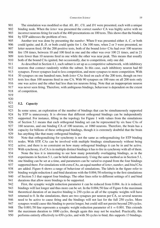
None the less it is interesting to see how many potentially overlapping bindings, as in theexperiments in Section 5.1, can be held simultaneously. Using the same method as in Section 5.1,one binding can be set at a time, and parameters can be varied to expand from the four bindingssupported there. For simulations with extra CAs, an equal number of letter, number, and bind CAsare added. Figure 6 shows a range of behaviour of simulations. The labels in the figure refer tobinding weight reduction k and bind durations with the 0.004/50 referring to the first simulationsof Section 5.1 that support four bindings. The other lines refer to different settings of k and binddurations that allow more bindings to be supported.

First, the synaptic weight reduction parameter k can be reduced from 0.004. As it is reduced,bindings will last longer and thus more can be set. In the 0.004/50 line of Figure 6 the maximumtheoretical duration of an inactive binding is 250 cycles as all of the synaptic weights will havereturned to 0. In the simulations, there are two synapses per neuron per CA, so several neuronsneed to be active to cause firing and the bindings will not last for the full 250 cycles. Moresynapses would cause this binding to persist longer, but could still not persist beyond 250 cycles.The 0.001/50 line represents a synaptic weight reduction parameter of k = 0.001. This extendsthe maximum duration to 1000 cycles, though again this may not be reached. Practically, thisperforms entirely effectively to 650 cycles, and with 50 cycles to bind, this supports 13 bindings.

9519529539549559569579589599609619629639649659669679689699709719729739749759769779789799809819829839849859869879889899909919929939949959969979989991000

20 C.R. Huyck

0

0.2

0.4

0.6

0.8

1

0 100 200 300 400 500 600 700 800

CorrectBindings

Simulation Cycle

.004/50

.004/20

.001/50

.002/20

Figure 6. Duration of bindings via STP varying by reduction rate and time to bind.

Similarly, reducing bind time increases the bindings that can be maintained. With a learningweight of 0.1, 10 cycles are the minimum to fully bind. The 0.004/20 line in the figure representsa bind epoch of 20 cycles. This has the same maximum duration of 250 cycles, but more bindingscan be supported over this time. There is theoretical limit of 10 bindings, but 7 are maintainedperfectly.

Reduced bind time and smaller synaptic weight reduction combine multiplicatively. The0.002/20 line in Figure 6 theoretically supports 20 bindings, four times two for the synapticweight reduction parameter times 50/20 for the bind time. Practically it is supporting 15 perfectlyeffectively. A further set of simulations was run with 0.001/20 (not shown in figure). This shows30 bindings being supported perfectly.

There is evidence that STP can last over 30 s (Varela, Sen, Gibson, Abbott, and Nelson 1997),which is 3000 cycles in the model. With 10 presentations to bind, 300 overlapping bindings cantheoretically be supported simultaneously following the above binding setting mechanism.

5.3. Compositionality

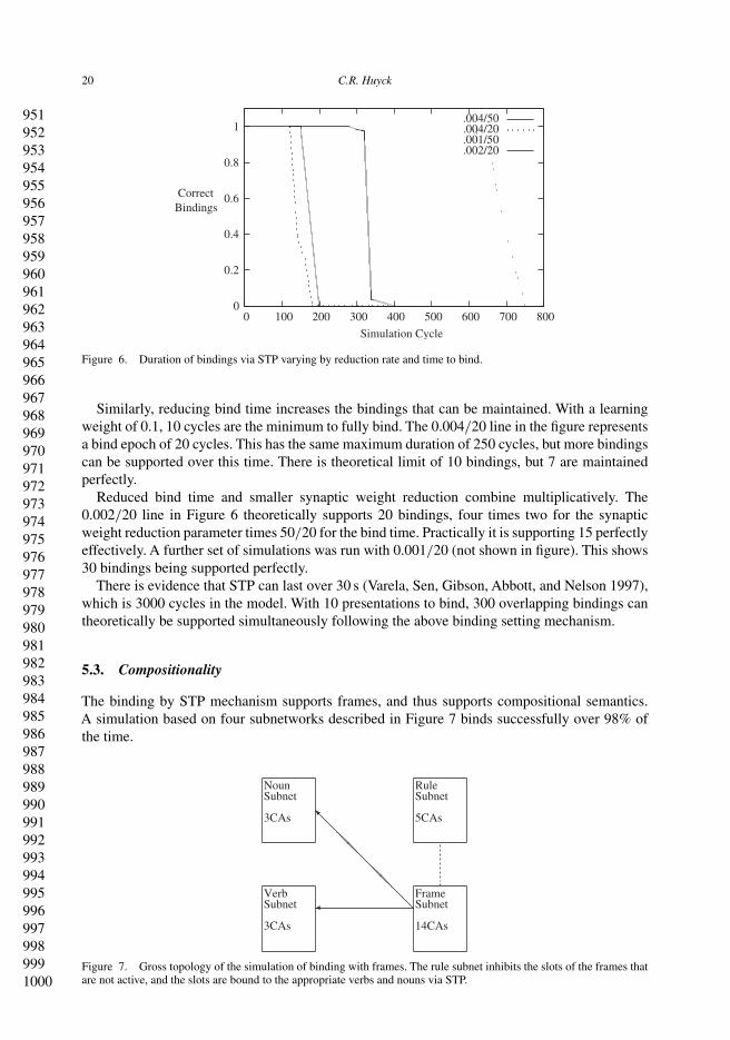
The binding by STP mechanism supports frames, and thus supports compositional semantics.A simulation based on four subnetworks described in Figure 7 binds successfully over 98% ofthe time.

NounSubnet

3CAs

RuleSubnet

5CAs

VerbSubnet

3CAs

FrameSubnet

14CAs

Figure 7. Gross topology of the simulation of binding with frames. The rule subnet inhibits the slots of the frames thatare not active, and the slots are bound to the appropriate verbs and nouns via STP.

10011002100310041005100610071008100910101011101210131014101510161017101810191020102110221023102410251026102710281029103010311032103310341035103610371038103910401041104210431044104510461047104810491050

Connection Science 21

The four subnets are the Verb, Noun, Rule, and Frame subnets. The Verb and Noun subnet consistof three CAs each of 160 neurons each representing a word; the Rule subnet of five CAs each of800 neurons each representing a rule; and the Frame net consists of 14 CAs each of 100 neuronswhich represent two frames each of seven slots. The constants were again the same as those forthe base subnets in Table 1 (θ = 4, D = 1.5, Fc = 1.0, Fr = 2.0,WB = 21, and P = 1.3).

As in the earlier simulations, connectivity within each subnet was distance biased with 80–20excitatory to inhibitory neurons. In the Frame subnet this was extended with synapses that learnvia the STP rule. Each frame consisted of seven slots, so the simulation has two frames. The baseslot was connected to the frame’s other slots, and, as in the simulations from Section 5.1, each ofthe neurons had two fast bind synapses to each of the appropriate CAs, along with the existingsynapses. The sentential complement slot had fast-bind synapses within the Frame subnet (seebelow).

Connectivity between the subnets was from the Frame subnet to the Verb and Noun subnets,represented by the arrows in Figure 7; and from the Rule subnet to the Frame subnet, representedby the dashed line. Each frame consisted of seven slots: base, base verb, actor, object, location,instrument, and sentential complement. The actor, object, and location slots had connectionsto each of the nouns, and the base verb slot had connections to each of the verbs. Each of theexcitatory neurons had two synapses to each of the appropriate CAs, and these synapses aremodified by the STP rule. The sentential complement slot was also connected to the base slotof the other frame in the same fashion as the other slots were connected to nouns and verbs.The instrument slot was not used in this simulation.

The rules inhibited the frame slots that were incompatible. Each inhibitory neuron had 15connections to each of those slots, and the rule CAs had 800 neurons to provide sufficient inhibitionto prevent those slots from igniting even when bound.

As in the earlier simulations the net was trained by 20 presentations of 50 cycles for each ofthe base CAs. As the rule CAs were 800 neurons, 400 neurons were presented during traininginstead of 50 for CAs in the other nets.

The relevant binding parameters are 20 cycles and k = 0.004. Binding was done by framesthat correlated to the sentences Jody loves Pat., Pat loves Jody., Pat went to the store, and Jodysaid Pat went to the store. This was done by presenting the appropriate rule, slot and filler. Forexample, the verb love, the first frame’s base slot, the first frame’s base verb slot, and the start VPrule were presented for 20 cycles. For the first three sentences this was three presentations; forJody loves Pat:

(1a) the first frame’s base and base verb, verb love, and the start VP rule;(1b) the first frame’s base and actor slot, noun Jody, and add actor rule;(1c) the first frame’s base and object slot, noun Pat, and add object rule;

The second sentence inverted the actor and object; the third used the verb go and replaced theobject rule and slot with location, and used the noun store. For the fourth sentence there was sevenpresentations:

(4a) the first frame’s base and base verb, verb said, and the start VP rule;(4b) the first frame’s base and actor slot, noun Jody, and add actor rule;(4c) the first frame’s base and scomp, and add scomp rule;(4d) the first frame’s scomp, second frame’s base, and add scomp rule;(4e) the second frame’s base and base verb, verb went and the start VP rule;(4f )the second frame’s base and actor slot, noun Pat, and add actor rule;(4g) the second frame’s base and location slot, noun store, and add location rule.

10511052105310541055105610571058105910601061106210631064106510661067106810691070107110721073107410751076107710781079108010811082108310841085108610871088108910901091109210931094109510961097109810991100

22 C.R. Huyck

The complete test was done in three phases. The first phase bound the slots for Jody loves Pat.into the first frame. There was then a period of erasing of 250 cycles. The second phase bound theslots for Pat loves Jody. into the first frame and the slots for Pat went to the store. into the secondframe. There was then another period of erasing followed by the slots for Jody said Pat went tothe store. being bound into the first and second frame.

Testing followed the phases before erasing. Testing was done by presenting the base frame slotand the rule. The simulation was run on 10 different nets and each net did all three phases 10times. The correct binding was considered to have occurred if more than 10 neurons in the correctnode were firing in the 19th cycle after presentation; no incorrect binding was considered to haveoccurred if no other neuron in the appropriate net fired. For any given run, there were 14 possiblecorrect bindings, and 13 possible incorrect bindings (the sentential complement could not havegotten the wrong base frame as both should be active). All of the correct bindings were formed andin 1290 of the 1300 runs no incorrect bindings occurred. This gives a Bound/Unbound/F-Scoreresult of 100%/99.2%/99.6%. Note that the failures that occurred all occurred within one nettowards the end of the run, and were based on the base frame slot CAs recruiting each other viaLTP.

A sentence is represented by a verb frame that has slots that are dynamically filled. Pat loves Jody.includes the semantics of Pat, love and Jody, and is different from Jody loves Pat. The simulationshows the difference between these two sentences and shows that frames can be implemented bySTP. Similarly, the simulation of the semantic representation of Pat went to the store. shows thatextra slots can be added seamlessly, and that multiple sentences can be stored simultaneously.

The phenomena is recursive. The simulation of the sentence Jody said Pat went to the store.shows that verb frames can be slot fillers. There is no theoretical limitation to the depth froma psycholinguistic standpoint. From a simulation standpoint, reactivation of bindings might benecessary during parsing to support the bindings, but Section 5.2 shows how 300 bindings mightbe stored without recourse to separation.

CAs are associative structures but frames are relational. This difference is bridged, above, byfast-bind connections. Initially, the frame is represented by the base slot, and the remaining slotsare inactive. As slots are filled, the base slot and the particular slots are coactive; STP causes themto be bound so the base slot will activate the bound slots, but not the unbound slots. In the test,the unbound slots are explicitly activated via external activation.

A more sophisticated framing mechanism has been used in a natural language parser (Huyck2009). This parser uses frames for both Noun and Verb phrases because both can have others ascomponents. Rules no longer suppress frames, but instead activate particular slots in combinationwith existing activation. The parser is stackless and follows other psycholinguistic models (Lewisand Vasishth 2005).

When multiple rules are applicable because of simultaneous activation, competition via inhi-bition selects the rule to apply. For instance, when parsing a simple sentence like I saw. two itemsare active the NP I and the VP saw. Two rules are also applicable the AddActor rule and theAddObject rule. The VP is more active since it has been more recently activated, so the AddActorrule wins and is applied. Once a slot is bound, it is marked as bound (neurally) and cannot berebound. In more complex sentences, several frames can be simultaneously active. In Pat saidgo to the store yesterday. The frames VP1 said actor-Pat scomp VP2, VP2 go loc-to-store, PP1to-store, and NP3 yesterday are all simultaneously active; the NP1 Pat frame is inactive sinceit can no longer be modified. The rule that adds yesterday as the time of VP1 will activate theappropriate slot in that frame and the binding will be complete; the other two frames VP2 andPP1 are already bound. The rule causes the binding, but the binding persists after the rule ceasesfiring.

It is fair to note that during parsing of a sentence, multiple constituents may be simultaneouslyactive. Only the appropriate items must be used to fill the appropriate slots. Binding by STP has

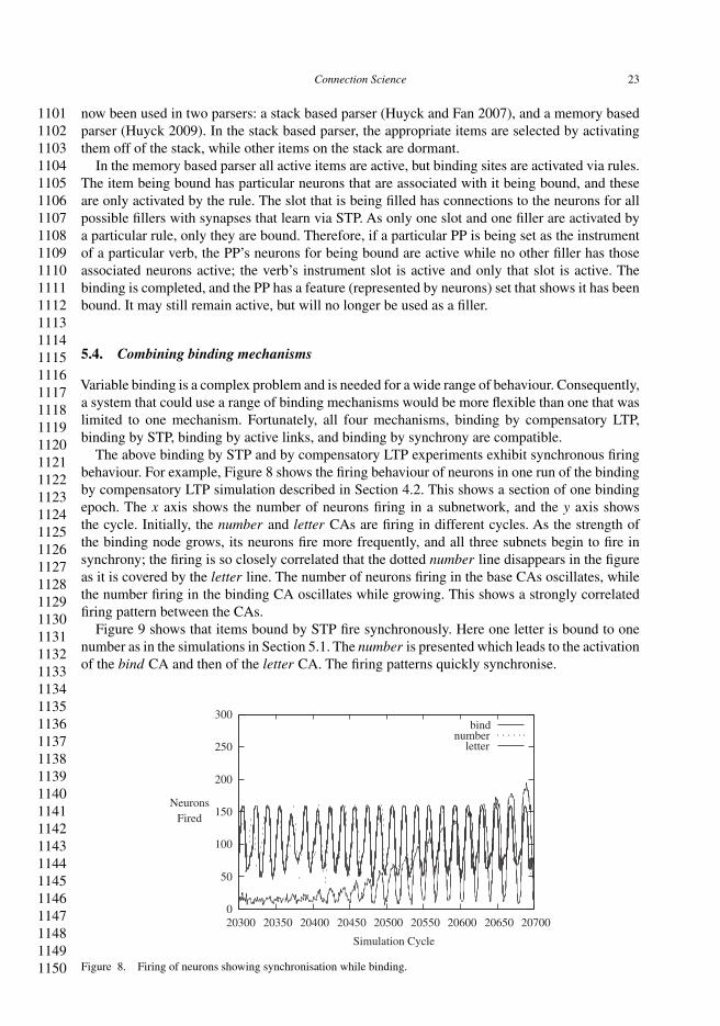
11011102110311041105110611071108110911101111111211131114111511161117111811191120112111221123112411251126112711281129113011311132113311341135113611371138113911401141114211431144114511461147114811491150

Connection Science 23

now been used in two parsers: a stack based parser (Huyck and Fan 2007), and a memory basedparser (Huyck 2009). In the stack based parser, the appropriate items are selected by activatingthem off of the stack, while other items on the stack are dormant.

In the memory based parser all active items are active, but binding sites are activated via rules.The item being bound has particular neurons that are associated with it being bound, and theseare only activated by the rule. The slot that is being filled has connections to the neurons for allpossible fillers with synapses that learn via STP. As only one slot and one filler are activated bya particular rule, only they are bound. Therefore, if a particular PP is being set as the instrumentof a particular verb, the PP’s neurons for being bound are active while no other filler has thoseassociated neurons active; the verb’s instrument slot is active and only that slot is active. Thebinding is completed, and the PP has a feature (represented by neurons) set that shows it has beenbound. It may still remain active, but will no longer be used as a filler.

5.4. Combining binding mechanisms

Variable binding is a complex problem and is needed for a wide range of behaviour. Consequently,a system that could use a range of binding mechanisms would be more flexible than one that waslimited to one mechanism. Fortunately, all four mechanisms, binding by compensatory LTP,binding by STP, binding by active links, and binding by synchrony are compatible.

The above binding by STP and by compensatory LTP experiments exhibit synchronous firingbehaviour. For example, Figure 8 shows the firing behaviour of neurons in one run of the bindingby compensatory LTP simulation described in Section 4.2. This shows a section of one bindingepoch. The x axis shows the number of neurons firing in a subnetwork, and the y axis showsthe cycle. Initially, the number and letter CAs are firing in different cycles. As the strength ofthe binding node grows, its neurons fire more frequently, and all three subnets begin to fire insynchrony; the firing is so closely correlated that the dotted number line disappears in the figureas it is covered by the letter line. The number of neurons firing in the base CAs oscillates, whilethe number firing in the binding CA oscillates while growing. This shows a strongly correlatedfiring pattern between the CAs.

Figure 9 shows that items bound by STP fire synchronously. Here one letter is bound to onenumber as in the simulations in Section 5.1. The number is presented which leads to the activationof the bind CA and then of the letter CA. The firing patterns quickly synchronise.

0

50

100

150

200

250

300

20300 20350 20400 20450 20500 20550 20600 20650 20700

NeuronsFired

Simulation Cycle

bindnumber

letter

Figure 8. Firing of neurons showing synchronisation while binding.

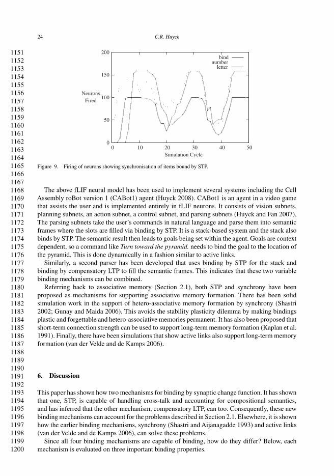
11511152115311541155115611571158115911601161116211631164116511661167116811691170117111721173117411751176117711781179118011811182118311841185118611871188118911901191119211931194119511961197119811991200

24 C.R. Huyck

0

50

100

150

200

0 10 20 30 40 50

NeuronsFired

Simulation Cycle

bindnumber

letter

Figure 9. Firing of neurons showing synchronisation of items bound by STP.

The above fLIF neural model has been used to implement several systems including the CellAssembly roBot version 1 (CABot1) agent (Huyck 2008). CABot1 is an agent in a video gamethat assists the user and is implemented entirely in fLIF neurons. It consists of vision subnets,planning subnets, an action subnet, a control subnet, and parsing subnets (Huyck and Fan 2007).The parsing subnets take the user’s commands in natural language and parse them into semanticframes where the slots are filled via binding by STP. It is a stack-based system and the stack alsobinds by STP. The semantic result then leads to goals being set within the agent. Goals are contextdependent, so a command like Turn toward the pyramid. needs to bind the goal to the location ofthe pyramid. This is done dynamically in a fashion similar to active links.

Similarly, a second parser has been developed that uses binding by STP for the stack andbinding by compensatory LTP to fill the semantic frames. This indicates that these two variablebinding mechanisms can be combined.

Referring back to associative memory (Section 2.1), both STP and synchrony have beenproposed as mechanisms for supporting associative memory formation. There has been solidsimulation work in the support of hetero-associative memory formation by synchrony (Shastri2002; Gunay and Maida 2006). This avoids the stability plasticity dilemma by making bindingsplastic and forgettable and hetero-associative memories permanent. It has also been proposed thatshort-term connection strength can be used to support long-term memory formation (Kaplan et al.1991). Finally, there have been simulations that show active links also support long-term memoryformation (van der Velde and de Kamps 2006).

6. Discussion

This paper has shown how two mechanisms for binding by synaptic change function. It has shownthat one, STP, is capable of handling cross-talk and accounting for compositional semantics,and has inferred that the other mechanism, compensatory LTP, can too. Consequently, these newbinding mechanisms can account for the problems described in Section 2.1. Elsewhere, it is shownhow the earlier binding mechanisms, synchrony (Shastri and Aijanagadde 1993) and active links(van der Velde and de Kamps 2006), can solve these problems.

Since all four binding mechanisms are capable of binding, how do they differ? Below, eachmechanism is evaluated on three important binding properties.

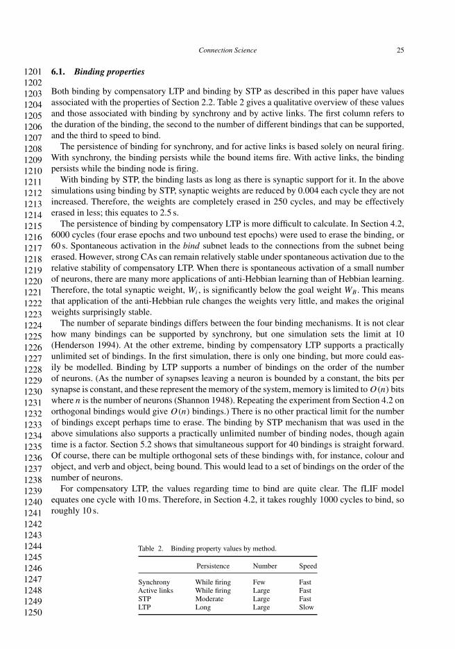
12011202120312041205120612071208120912101211121212131214121512161217121812191220122112221223122412251226122712281229123012311232123312341235123612371238123912401241124212431244124512461247124812491250

Connection Science 25

6.1. Binding properties

Both binding by compensatory LTP and binding by STP as described in this paper have valuesassociated with the properties of Section 2.2. Table 2 gives a qualitative overview of these valuesand those associated with binding by synchrony and by active links. The first column refers tothe duration of the binding, the second to the number of different bindings that can be supported,and the third to speed to bind.

The persistence of binding for synchrony, and for active links is based solely on neural firing.With synchrony, the binding persists while the bound items fire. With active links, the bindingpersists while the binding node is firing.

With binding by STP, the binding lasts as long as there is synaptic support for it. In the abovesimulations using binding by STP, synaptic weights are reduced by 0.004 each cycle they are notincreased. Therefore, the weights are completely erased in 250 cycles, and may be effectivelyerased in less; this equates to 2.5 s.

The persistence of binding by compensatory LTP is more difficult to calculate. In Section 4.2,6000 cycles (four erase epochs and two unbound test epochs) were used to erase the binding, or60 s. Spontaneous activation in the bind subnet leads to the connections from the subnet beingerased. However, strong CAs can remain relatively stable under spontaneous activation due to therelative stability of compensatory LTP. When there is spontaneous activation of a small numberof neurons, there are many more applications of anti-Hebbian learning than of Hebbian learning.Therefore, the total synaptic weight, Wi , is significantly below the goal weight WB . This meansthat application of the anti-Hebbian rule changes the weights very little, and makes the originalweights surprisingly stable.

The number of separate bindings differs between the four binding mechanisms. It is not clearhow many bindings can be supported by synchrony, but one simulation sets the limit at 10(Henderson 1994). At the other extreme, binding by compensatory LTP supports a practicallyunlimited set of bindings. In the first simulation, there is only one binding, but more could eas-ily be modelled. Binding by LTP supports a number of bindings on the order of the numberof neurons. (As the number of synapses leaving a neuron is bounded by a constant, the bits persynapse is constant, and these represent the memory of the system, memory is limited to O(n) bitswhere n is the number of neurons (Shannon 1948). Repeating the experiment from Section 4.2 onorthogonal bindings would give O(n) bindings.) There is no other practical limit for the numberof bindings except perhaps time to erase. The binding by STP mechanism that was used in theabove simulations also supports a practically unlimited number of binding nodes, though againtime is a factor. Section 5.2 shows that simultaneous support for 40 bindings is straight forward.Of course, there can be multiple orthogonal sets of these bindings with, for instance, colour andobject, and verb and object, being bound. This would lead to a set of bindings on the order of thenumber of neurons.

For compensatory LTP, the values regarding time to bind are quite clear. The fLIF modelequates one cycle with 10 ms. Therefore, in Section 4.2, it takes roughly 1000 cycles to bind, soroughly 10 s.

Table 2. Binding property values by method.

Persistence Number Speed

Synchrony While firing Few FastActive links While firing Large FastSTP Moderate Large FastLTP Long Large Slow

12511252125312541255125612571258125912601261126212631264126512661267126812691270127112721273127412751276127712781279128012811282128312841285128612871288128912901291129212931294129512961297129812991300

26 C.R. Huyck

Compared with this, binding via STP is quite rapid. In the simulations in Sections 4.3 and 5the learning rate is set to 0.1 and the weight is clipped at 1; so binding happens in 10 cycles, andthis equates to times about 100 ms. This contradicts the statement ‘it is unlikely that there existmechanisms that support widespread structural changes and growth of new links within’hundredsof ms (Shastri and Aijanagadde 1993). There is biological evidence of STP based on short burstsof spikes that persist for seconds to minutes (Hempel et al. 2000).

There is a vast range of evidence for synaptic changes of short duration (see Zucker and Regehr(2002) for a review), and there are a wide range of behaviours, including different behaviours forneurons in different portions of the brain (Castro-Alamancos and Connors 1997). Evidence showsthat short-term synaptic change can persist from under a second to over 30 (Varela et al. 1997).It has been shown that as few as 10 spikes at 50 Hz can lead to STP of synapses (Tecuapetla,Crillo-Reid, Bargas, and Galarraga 2007). In the simulations described in this paper, that wouldbe 10 sets of neural firings in alternating cycles. For all that is known to the contrary, it is possiblethat the relevant form of rapid binding could be implemented by synaptic change. Bursts of 100 Hzfirings for as little as 300 ms. leads to STP that endures for tens of minutes (Schulz and Fitzgibbons1997).

It should also be noted that the time courses of the binding by STP and binding by compensatoryLTP are affected by the constants, topologies, and presentation mechanics. The above simulationsprovide example time courses.

Binding by synchrony can occur in tens of ms (Wennekers and Palm 2000). As active linkstake only a few neural firings to form a binding, they too should occur on the order of tens of ms(van der Velde and de Kamps 2006).

A related property is the number of items per binding. The compensatory LTP mechanismlimits this, but binding by STP and binding by synchrony do not. Binding by active links allowsthe developer to program this.

6.2. Maintaining binding by firing vs. by synapses

It has been stated that ‘the number of dynamic bindings expressed via some form of activity(e.g. synchrony) will be comparable with the number of ignited (fired) CAs’. If bindings aremaintained by neural firing, this is the case, so it is the case for both binding by synchrony andactive links. However, if binding is done by synaptic modification, CAs do not need to be activeto remain bound; consequently, synaptic modification allows a much larger range of bindings tobe supported.

If all of the bound items remain active, as in synchrony, or all of the binding nodes remain active,as in active links, a large number of items are active. This can lead to problems of crosstalk. Thesecan be addressed programmatically, but it is clearly useful to be able to deactivate CAs and retainbindings.

Furthermore, maintaining a binding created by synaptic change, requires fewer neurons firing,and neural firing is biologically expensive (Attwell and Laughlin 2001; Aiello and y Rita 2002).Maintaining bindings by firing is thus biologically expensive. It costs a lot of energy.

Therefore, binding by firing may be useful, but it comes at a cost. However, binding by synapticchange has to pay much less.

6.3. Binding and memory

The three properties, speed to bind, number of bindings supported, and speed to unbind are alsoissues of general memory formation. Recall that CAs give an explanation for short-term memory(CA activation and persistence) and long-term memory (stable state CA formation based on LTP).

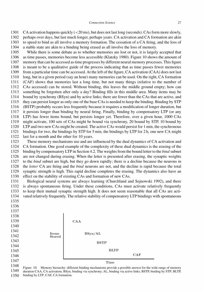
13011302130313041305130613071308130913101311131213131314131513161317131813191320132113221323132413251326132713281329133013311332133313341335133613371338133913401341134213431344134513461347134813491350

Connection Science 27

CA activation happens quickly (<20 ms), but does not last long (seconds). CAs form more slowly,perhaps over days, but last much longer, perhaps years. CA activation and CA formation are akinto speed to bind as all involve a memory formation. The cessation of a CA firing, and the loss ofa stable state are akin to a binding being erased as all involve the loss of memory.

While there is some debate as to whether memories are lost or not, it is largely accepted thatas time passes, memories become less accessible (Klatzky 1980). Figure 10 shows the amount ofmemory that can be accessed as time progresses by different neural memory processes. This figureis meant to be a qualitative guide of the process indicating that as time passes fewer memoriesfrom a particular time can be accessed. At the left of the figure, CA activation (CAA) does not lastlong, but in a given period (say an hour) many memories can be used. On the right, CA formation(CAF) shows that memories last a long time, but not many things (relative to the number ofCAs accessed) can be stored. Without binding, this leaves the middle ground empty; how cansomething be forgotten after only a day? Binding fills in this middle area. Many items may bebound by synchrony (BSyn) and by active links; there are fewer than the CAs that are active, andthey can persist longer as only one of the base CAs is needed to keep the binding. Binding by STP(BSTP) probably occurs less frequently because it requires a modification of longer duration, butit persists longer than binding by neural firing. Finally, binding by compensatory LTP (or anyLTP) has fewer items bound, but persists longer yet. Therefore, over a given hour, 1000 CAsmight activate, 100 sets of CAs might be bound via synchrony, 20 bound by STP, 10 bound byLTP and two new CAs might be created. The active CAs would persist for 1 min, the synchronousbindings for two, the bindings by STP for 5 min, the bindings by LTP for 2 h, one new CA mightlast for a month and the other for 10 years.

These memory mechanisms use and are influenced by the dual dynamics of CA activation andCA formation. One good example of the complexity of these dual dynamics is the erasing of thebinding by compensatory LTP in Section 4.2. The weights from the bound letter to the bind subnetare not changed during erasing. When the letter is presented after erasing, the synaptic weightsto the bind subnet are high, but they go down rapidly; there is a decline because the neurons inthe letter CA are firing and the bind neurons are not, and the decline is rapid because the totalsynaptic strength is high. This rapid decline completes the erasing. The dynamics also have aneffect on the stability of existing CAs and formation of new CAs.

Biological neural systems are always learning (Churchland and Sejnowski 1992), and thereis always spontaneous firing. Under these conditions, CAs must activate relatively frequentlyto keep their mutual synaptic strength high. It does not seem reasonable that all CAs are acti-vated relatively frequently. The relative stability of compensatory LTP bindings with spontaneous

Figure 10. Memory hierarchy: different binding mechanisms provide a possible answer for the wide range of memoryduration CAA, CA activation; BSyn, binding via synchrony; AL, binding via active links; BSTP, binding by STP; BLTP,binding by LTP; CAF, CA formation.

13511352135313541355135613571358135913601361136213631364136513661367136813691370137113721373137413751376137713781379138013811382138313841385138613871388138913901391139213931394139513961397139813991400

28 C.R. Huyck

activation provides some hope that this problem may be resolved, but it has not yet been since thesystem either is stable without spontaneous activation, or plastic with, but in neither case both.

Binding by synchrony, active links, and STP have a lesser effect on CA stability and plasticity,but they still have an effect. They have less of an effect because they are not based on long-termsynaptic change. They still have an effect because they cause the simultaneous firing of neuronsin CAs, and this will lead to increased permanent synaptic weight between the bound CAs. Thismight lead to the CAs recruiting each other, so that they no longer can be independently active.

Binding by compensatory LTP can now be looked at as an associative memory mechanism.CAs that are frequently bound may become more related but, perhaps due to topology, may notrecruit each other. Other options for resolving stability problems include modified spontaneousactivation mechanisms, subassemblies, and learning rules involving fatigue. In the simulationsdescribed in this paper, spontaneous activation is purely random; this might be modified to makeneurons fire when they have not fired for a long time, and these neurons might co-fire based ontheir last activity. Subassemblies are merely sets of neurons that do not persist, but can be activatedby spontaneous activation leading to synaptic support. Finally, if synaptic weights only changedsignificantly when neurons were fatigued, spontaneous activation would have little effect on them.These mechanisms are, of course, speculative.

Binding by compensatory LTP, and to a lesser extent the other binding mechanisms, provides awindow into the stability plasticity dilemma of associative memory. It is relatively easy to modelthe indefinite storage of memories as once stored all memories are stable. When the memorystore is large, this may cause no obvious problems. However, access to all memories can not beretained, and access to psychological memories is lost on a range of scales. Perhaps binding bycompensatory LTP will provide an answer to how memories can be forgotten after days or years.

7. Conclusion

Binding is an important problem because a solution to it allows a system to have compositionalsyntax and semantics. This composition is necessary for a system to model the full range of humanbehaviour. If the particular problems of binding features in an object, frames, and rules can besolved, then a system can be built that is compositional.

This paper has introduced a new variable binding mechanism, binding by STP and made useof the relatively novel variable binding by compensatory LTP. Simulations have shown that thesemechanisms, like synchrony and active links, can bind features in an object, and implement rulesand frames. Simulations have shown that binding by STP also solves the problem of two and thatbinding by LTP should be able to.

Binding by STP is fast to bind, persists beyond the activity of the bound CAs, is relativelyeasy to engineer, and works consistently. Binding by compensatory LTP works, but faces thestability plasticity dilemma. It is slower to bind and the bindings persist longer. Neither of thesemechanisms faces a combinatorial explosion to bind items, and both can support a very largenumber of bindings.

Binding via compensatory LTP and by STP can be used together and with the earlier definedbinding mechanisms, binding via synchrony and binding by active links, to complement eachother. They each have different behaviours on time to bind, time to erase, and capacity. Alongwith CA activation and CA formation, these binding mechanisms give a wide range of memoryformation and retention behaviour.

Together, these mechanisms allow for a sophisticated use of compositional syntax and semanticsin a simulated neural system. This will support the development of complex symbol processingagents from simulated neurons bridging the gap between subsymbolic and symbolic systems.

14011402140314041405140614071408140914101411141214131414141514161417141814191420142114221423142414251426142714281429143014311432143314341435143614371438143914401441144214431444144514461447144814491450

Connection Science 29

Acknowledgements

This work was supported by EPSRC grant GR/R13975/01 and EP/D059720. Thanks go to Dan Diaper, ThomasWennekers, Pieter DeVries, Stephen Kaplan and the SESAME group, and anonymous reviewers for comments on thisarticle.

References

Abeles, M. (1991), Corticonics: Neural Circuits of the Cerebral Cortex, Cambridge University Press. Q2Abeles, M., Bergman, H., Margalit, E., and Vaddia, E. (1993), ‘Spatiotemporal Firing Patterns in the Frontal Cortex of

Behaving Monkeys’, Journal of Neurophysiology, 70(4), 1629–1638.Ackley, D., Hinton, G., and Sejnowski, T. (1985), ‘A Learning Algorithm for Boltzmann Machines’, Cognitive Science,

9, 147–169.Aiello, G., and y Rita, P.B. (2002), ‘The Cost of an Action Potential’, Journal of Neuroscience Methods, 103(2), 145–149.Amit, D. (1989), Modelling Brain Function: The World of Attractor Neural Networks, Cambridge University Press. Q2Amit, D., and Brunel, N. (1997), ‘Model of Global Spontaneous Activity and Local Structured Activity During Delay

Periods in the Cerebral Cortex’, Cerebral Cortex, 7, 237–252.Anderson, J., and Lebiere, C. (1998), The Atomic Components of Thought. Lawrence Erlbaum. Q2Attwell, D., and Laughlin, S. (2001), ‘An Energy Budget for Signaling in the Gray Matter of the Brain’, Journal of

Cereberal Blood Flow Metabolism, 21(10), 1133–1145.Bevan, M., and Wilson, C. (1999), ‘Mechanisms Underlying Spontaneous Oscillation and Rhythmic Firing in Rat

Subthalamic Neurons’, Neuroscience, 19, 7617–7628.Bienenstock, E., and Malsburg, C.V.D. (1987), ‘A Neural Network for Invariant Pattern Recognition’, Europhysics Letters,

4(1), 121–126.Braitenberg, V. (1989), ‘Some Arguments for a Theory of Cell Assemblies in the Cerebral Cortex’, in Neural Connections,

Mental Computation, eds. Nadel, Cooper, Culicover, and Harnish, MIT Press. Q3Browne, A., and Sun, R. (1999), ‘Connectionist Variable Binding’, Expert Systems, 16(3), 189–207.Brunel, N. (1996), ‘Hebbian Learning of Context in Recurrent Neural Networks’, Neural Computation, 8, 1677–1710.Buonomano, D. (1999), ‘Distinct Functional Types ofAssociative Long-term Potentiation in Neocortical and Hippocampal

Pyramidal Neurons’, Neuroscience, 19(16), 6748–6754.Carpenter, G., and Grossberg, S. (1988), ‘The Art of Adaptive Pattern Recognition by a Self-organizing Neural Network’,

IEEE Computer, 21, 77–88.Castro-Alamancos, M., and Connors, B. (1997), ‘Distinct Forms of Short-term Plasticity at Excitatory Synapses of

Hippocampus and Neocortex’, Proceedings of the National Academy of Sciences USA, 94, 4161–4166.Chacron, M., Pakdaman, K., and Longtin, A. (2003), ‘Interspike Interval Correlations, Memory, Adaptation, and

Refractoriness in a Leaky Integrate-and-fire Model with Threshold Fatigue’, Neural Computation, 15, 253–278.Churchland, P., and Sejnowski, T. (1992), The Computational Brain. MIT Press. Q2Dayan, P., and Abbott, L. (2005), Theoretical Neuroscience: Computational and Mathematical Modeling of Neural

Systems, MIT Press. Q2deVries, P. (2004), ‘Effects of Binding in the Identification of Objects’, Psychological Research, 69, 41–66.Eccles, J. (1986), ‘Chemical Transmission and Dale’s Principle’, Progress in Brain Research, 68, 3–13.Eckhorn, R., Bauer, R., Jordan, W., Brosch, M., Kruse, W., Munk, M., and Reitboeck, H. (1988), ‘Coherent Oscillations:

A Mechanism of Feature Linking in the Visual Cortex?’ Biological Cybernetics, 60, 121–130.Feldman, J. (1982), ‘Dynamic Connections in Neural Networks’, Biological Cybernetics, 46, 27–39.Filmore, C. (1968), ‘The Case for Case’, in Universals in Linguistic Theory, eds. E. Back and R. Harms, Holt, Rinheart

and Winston Inc. Q2Fodor, J., and Pylyshyn, Z. (1988), ‘Connectionism and Cognitive Architecture: A Criticial Analysis’, Cognition, 28,

3–71.Frixione, M., Spinelli, G., and Gaglio, S. (1989), ‘Symbols and Subsymbols for Representing Knowledge: A Catalogue

Raisonne’, in Proceedings of the Eleventh International Joint Conference on Artificial Intelligence, pp. 3–7.Furber, S., Bainbridge, W., Cumpstey, J., and Temple, S. (2004), ‘Sparse Distributed Memory Using n-of-m Codes’,

Neural Networks, 17(10), 1437–1451.Fusi, S. (2008), ‘A Quiescent Working Memory’, Science, 319, 1495–1496.Fusi, S., Drew, P., and Abbott, L. (2005), ‘Cascade Models of Synaptically Stored Memories’, Neuron, 45, 599–611.Gerstner, W., and Kistler, W. (2002), ‘Mathematical Formulations of Hebbian Learning’, Biological Cybernetics, 87,

404–415.Gerstner, W., and van Hemmen, J. (1992), ‘Associative Memory in a Network of Spiking Neurons’, Network, 3, 139–164.Gunay, C., and Maida, A. (2006), ‘Using Temporal Binding for Hierarchical Recruitment of Conjunctive Concepts Over

Delayde Lines’, Neurocomputing, 69, 317–367.Hadley, R. (2007), ‘Synchronous vs. Conjunctive Binding: A False Dichotomy?’ Connection Science, 19(2), 111–130.Harnad, S. (1990), ‘The Symbol Grounding Problem’, Physica D, 42, 335–346.Hebb, D.O. (1949), The Organization of Behavior, John Wiley and Sons. Q2Hempel, C., Hartman, K., Wang, X., Turrigiano, G., and Nelson, S. (2000), ‘Multiple Forms of Short-term Plasticity at

Excitatory in Rat Medial Prefrontal Cortex’, Journal of Neurophysiology, 83, 3031–3041.

14511452145314541455145614571458145914601461146214631464146514661467146814691470147114721473147414751476147714781479148014811482148314841485148614871488148914901491149214931494149514961497149814991500

30 C.R. Huyck

Henderson, J. (1994), ‘Connectionist Syntactic Parsing Using Temporal Variable Binding’, Journal of PsycholinguisticResearch, 23(5), 353–379.

Hodgkin, A., and Huxley, A. (1952), ‘A Quantitative Description of Membrane Current and Its Application to Conductionand Excitation in Nerve’, Journal of Physiology, 117, 500–544.

Hofstadter, D. (1979), Godel, Escher and Bach: An Eternal Golden Braid. Basic Books.Q2Hopcroft, J., and Ullman, J. (1979), Introduction to Automata Theory, Languages and Computation, Addison-Wesley.

Q2 Hopfield, J. (1982), ‘Neural Nets and Physical Systems with Emergent Collective Computational Abilities’, Proceedingsof the National Academy of Sciences USA, 79, 2554–2558.

Huyck, C. (2004), ‘Overlapping Cell Assemblies From Correlators’, Neurocomputing, 56, 435–439.Huyck, C. (2007), ‘Creating Hierarchical Categories Using Cell Assemblies’, Connection Science, 19(1), 1–24.Huyck, C. (2008), ‘Cabot1: A Videogame Agent Implemented in fLIF Neurons’, in IEEE Systems, Man and Cybernetics

Society.Q4Huyck, C. (2009), ‘A Psycholinguistic Model of Natural Language Parsing Implemented in Simulated Neurons,’Cognitive

Neurodynamics.Q4Huyck, C., and Belavkin, R. (2006), ‘Counting With Neurons: Rule Application With Nets of Fatiguing Leaky Integrate

and Fire Neurons’, in Proceedings of the Seventh International Conference on Cognitive Modelling, pp. 142–147.Huyck, C., and Bowles, R. (2004), ‘Spontaneous Neural Firing in Biological and Artificial Neural Systems’, Journal of

Cognitive Systems, 6(1), 31–40.Huyck, C., and Fan, Y. (2007), ‘Parsing With fLIF Neurons’, in IEEE Systems, Man and Cybernetics Society, pp. 35–40.Jackendoff, R. (2002), Foundations of Language: Brain, Meaning, Grammar, Evolution, Oxford University Press.Q2Kaplan, S.,Weaver, M., and French, R. (1990), ‘Active Symbols and Internal Models: Towards a Cognitive Connectionism’,

AI and Society, 4, 51–71.Kaplan, S., Sontag, M., and Chown, E. (1991), ‘Tracing Recurrent Activity in Cognitive Elements (TRACE): A Model of

Temporal Dynamics in a Cell Assembly’, Connection Science, 3, 179–206.Klatzky, R. (1980), Human Memory: Structures and Processes, W. H. Freeman and Co.Q2Knoblauch,A., and Palm, G. (2001), ‘Pattern Separation and Synchronization in SpikingAssociative Memories and Visual

Areas’, Neural Networks, 14, 763–780.Knoblauch, A., Markert, H., and Palm, G. (2004), ‘An Associative Model of Cortical Language and Action Processing’,

in Proceedings of the Ninth Neural Computation and Psychology Workshop, pp. 79–83.Laird, J., Newell, A., and Rosenbloom, P. (1987), ‘Soar: An Architecture for General Cognition’, Artificial Intelligence,

33, 1.Lansky, P., Sanda, P., and He, J. (2006), ‘The Parameters of the Stochastic Leaky Integrate-and-fire Neuronal Model’,

Journal of Computational Neuroscience, 21, 211–223.Lewis, R., and Vasishth, S. (2005), ‘An Activation-based Model of Sentence Processing as Skilled Memory Retrieval’,

Cognitive Science, 29(3), 375–419.Lindsey, R. (1988), ‘Can This Treatment Raise the Dead’, Behavioral and Brain Sciences, 11(1), 41–42.Maass, W., and Bishop, C. (2001), Pulsed Neural Networks, MIT Press.Q2Malsburg, C.V.D. (1981), ‘The Correlation Theory of Brain Function’, Technical Report, Dept. of Neurobiology, Max-

Planck-Institute for Biophyscial Chemistry.Malsburg, C.V.D. (1986), ‘Am I Thinking Assemblies?’ in Brain Theory, ed. G. Palm and A. Aertsen, Springer-Verlag,

pp. 161–176.Q2McCulloch,W., and Pitts,W. (1943), ‘A Logical Calculus of Ideas Immanent in NervousActivity’, Bulletin of Mathematical

Biophysics, 5, 115–133.Messinger, A., Squire, L., Zola, S., and Albright, T. (2005), ‘Neural Correlates of Knowledge: Stable Representation of

Stimulus Associations Across Variations in Behavioural Performance,’ Neuron, 48, 359–371.Miyashita, Y. (1988), ‘Neuronal Correlate of Visual Associative Long-term Memory in the Primate Temporal Cortex’,

Nature, 335, 817–820.Mongillo, G., Barak, O., and Tsodyks, M. (2008), ‘Synaptic Theory of Working Memory’, Science, 319, 1543–1546.Newell, A. (1990), Unified Theories of Cognition, Harvard University Press.Q2O’Neill, J., Senior, T.,Allen, K., Huxter, J., and Csicsvari, J. (2008), ‘Reactivation of Experience-dependent CellAssembly

Patterns in Hippocampus’, Nature Neuroscience, 11, 209–215.Pulvermuller, F. (1999), ‘Words in the Brain’s Language’, Behavioral and Brain Sciences, 22, 253–336.Quillian, M. (1967), ‘Word Concepts: A Theory of Simulation of Some Basic Semantic Capabilities’, Behavioral Science,

12, 410–30.Rumelhart, D., and McClelland, J. (1982), ‘An Interactive Activation Model of Context Effects in Letter Perception: Part

2. The Contextual Enhancement and Some Tests and Extensions of the Model’, Psychological Review, 89(1), 60–94.Rumelhart, D., and McClelland, J., (ed.) (1986), Parallel Distributed Processing, MIT Press.Q2Sakai, K., and Miyashita, Y. (1991), ‘Neural Organization for the Long-term Memory of Paired Associates’, Nature, 354,

152–155.Schank, R., and Abelson, R. (1977), Scripts, Plans, Goals and Understanding, Lawrence Erlbaum.Q2Schulz, P., and Fitzgibbons, J. (1997), ‘Differing Mechanisms of Expression for Short- and Long-term Potentiation’,

Journal of Neurophysiology, 78, 321–334.Shannon, C. (1948), ‘A Mathematical Theory of Communication’, Bell System Technical Journal, 27, 379–423.Shastri, L. (2002), ‘A Computationally Efficient Abstraction of Long-term Potentiation’, Neurocomputing, 44–46, 33–41.Shastri, L. (2006), ‘Comparing the Neural Blackboard and the Temporal Synchrony Based SHRUTI Architectures’,

Behaviour and Brain Science, 29, 84–86.

15011502150315041505150615071508150915101511151215131514151515161517151815191520152115221523152415251526152715281529153015311532153315341535153615371538153915401541154215431544154515461547154815491550

Connection Science 31

Shastri, L., and Aijanagadde, V. (1993), ‘From Simple Associations to Systematic Reasoning: A Connectionist Represen-tation of Rules, Variables, and Dynamic Bindings Using Temporal Synchrony’, Behaviour and Brain Science, 16,417–494.

Shieber, S. (1986), An Introduction to Unification-Based Approaches to Grammar, Center for the Study of Language andInformation. Q2

Siegelmann, H., and Sontag, E. (1991), ‘On the Computational Power of Neural Nets’, Technical Report, SYCON.Smolensky, P. (1987), ‘Connectionist AI, Symbolic AI, and the Brain’, Artificial Intelligence Review, 1, 95–109.Smolensky, P. (1990), ‘Tensor Product Variable Binding and the Representation of Symbolic Structures in Connectionist

Systems’, Artificial Intelligence, 46, 159–216.Sompolinsky, H. (1987), ‘The Theory of Neural Networks: The Hebb Rule and Beyond’, in Proceedings of Heidelberg

Colloquium on Glassy Dynamics. Q5Sougne, J. (2001), ‘Binding and Multiple Instantiation in a Distributed Network of Spiking Neurons’, Connection Science,

13, 99–126.Tecuapetla, F., Crillo-Reid, L., Bargas, J., and Galarraga, E. (2007), ‘Dopaminergic Modulation of Short-term Synaptic

Plasticity at Striatal Inhibitory Synapses’, Proceedings of the National Academy of Sciences USA, 104(24), 10258–10263.

Usher, M., and Donnelly, N. (1998), ‘Visual Synchrony Affects Binding and Segmentation in Perception’, Nature, 394,179–182.

Valiant, L. (2005), ‘Memorization and Association on a Realistic Neural Model’, Neural Computation, 17, 527–555.van der Velde, F., and de Kamps, M. (2006), ‘Neural Blackboard Architectures of Combinatorial Structures in Cognition’,

Behavioral and Brain Sciences, 29, 1–72.Varela, J., Sen, K., Gibson, J., Abbott, L., and Nelson, S. (1997), ‘A Quantitative Description of Short-term Plasticity at

Excitatory Synapses in Layer 2/3 of Rat Primary Visual Cortex’, Journal of Neuroscience, 17, 7926–7940.Wennekers, T., and Palm, G. (2000), ‘Cell Assemblies, Associative Memory and Temporal Structure in Brain Signals’, in

Time and the Brain: Conceptual Advances in Brain Research (Vol. 2), ed. R. Miller, Harwood Academic Publishers,pp. 251–274. Q2

White, G., Levy, W., and Steward, O. (1988), ‘Evidence that Associative Interactions Between Afferents During theInduction of Long-term Potentiation Occur Within Local Dendritic Domains’, Proceedings of the National Academyof Sciences USA, 85, 2368–2372.

Willshaw, D., Buneman, O., and Longuet-Higgins, H. (1969), ‘Non-holographic Associative Memory’, Nature, 222,960–962.

Zucker, R., and Regehr, W. (2002), ‘Short-term Synaptic Plasticity’, Annual Review of Physiology, 64, 355–405.