Journal of Accounting and Economics 64 (2017) 123–149

Contents lists available at ScienceDirect

Journal of Accounting and Economics

journal homepage: www.elsevier.com/locate/jacceco

Employee quality and financial reporting outcomes

�

Andrew C. Call a , ∗, John L. Campbell b , Dan S. Dhaliwal c , 1 , James R. Moon Jr. d

a School of Accountancy, W.P. Carey School of Business, Arizona State University, United States b J.M. Tull School of Accounting, Terry College of Business, University of Georgia, United States c Department of Accounting, Eller College of Business, University of Arizona, United States d School of Accountancy, J. Mack Robinson College of Business, Georgia State University, United States

a r t i c l e i n f o

Article history:

Received 18 August 2015

Revised 8 June 2017

Accepted 12 June 2017

Available online 15 June 2017

Keywords:

employee characteristics

employee quality

education

financial reporting quality

a b s t r a c t

We examine the association between employee quality and financial reporting outcomes.

Using the average workforce education level in MSA(s) where the firm operates as a proxy

for employee quality, we find that firms with a high-quality workforce exhibit higher ac-

cruals quality, fewer internal control violations, and fewer restatements. These firms also

issue superior management forecasts, in terms of frequency, timeliness, accuracy, preci-

sion, and bias. Employees located at the firm’s headquarters primarily drive our findings.

Our evidence suggests employee quality, particularly at a firm’s headquarters, is associated

with both mandatory and voluntary disclosure quality.

© 2017 Elsevier B.V. All rights reserved.

“Educate and inform the whole mass of the people… They are the only sure reliance for the preservation of our liberty .”

Thomas Jefferson, 1787

1. Introduction

Following a series of accounting scandals in the early 20 0 0s (e.g., Enron and WorldCom), capital market participants

questioned how auditors and regulators failed to identify the misreporting. However, in a comprehensive examination of

fraud cases from 1996 to 2004, Dyck et al. (2010) find that a firm’s employees identify and reveal fraud more often (17%

of the time) than both auditors (10%) and the corporate finance division of the Securities and Exchange Commission (SEC)

(7%). Given that employees provide ex-post discipline of financial reporting by helping uncover fraud after it has occurred,

a natural question is whether employees are able to impose ex-ante discipline on financial reporting before violations take

place.

� We thank an anonymous reviewer, Anwer Ahmed, Kris Allee, Bruce Billings, Allen Blay, Dane Christensen, James Chyz, Matt Ege, Enrique Gomez, Frank

Heflin, David Koo, Phil Lamoreaux, Josh Lee, Landon Mauler, Sean McGuire, Rick Mergenthaler, Rick Morton, Spencer Pierce, Santhosh Ramalingegowda,

Stephanie Rasmussen, Lynn Rees, John Robinson, Sarah Shaikh, Nate Sharp, Laura Swenson, Jake Thornock, Senyo Tse, Connie Weaver, Ben Whipple, Joanna

Wu (the Editor), Holly Yang, Eric Yeung, and Tim Zhang for helpful comments and suggestions. We also appreciate comments from workshop partici-

pants at Georgia State University, Florida State University, National University of Singapore, Texas A&M University, the AAA 2015 annual meeting, the 2015

Brigham Young University Accounting Research Symposium, the AAA 2016 FARS mid-year meeting, and the doctoral students in James Chyz’s seminar at

the University of Tennessee. Andy Call, John Campbell, and Robbie Moon acknowledge the profound impact Dan Dhaliwal had on them both professionally

and personally. ∗ Corresponding author.

E-mail address: andycall@ASU.edu (A.C. Call). 1 Deceased.

http://dx.doi.org/10.1016/j.jacceco.2017.06.003

0165-4101/© 2017 Elsevier B.V. All rights reserved.

124 A.C. Call et al. / Journal of Accounting and Economics 64 (2017) 123–149

We examine whether the quality of a firm’s workforce is associated with financial reporting quality. We proxy for the

quality of a firm’s workforce in two ways: (1) the average education level of the workforce in the Metropolitan Statistical

Area (MSA) where the firm is headquartered, and (2) the average education level of the workforce across all MSAs mentioned

in the firm’s Form 10-K filing. 2 Using these measures, we examine two broad research questions. First, are highly educated

employees associated with improved mandatory disclosure quality? Second, are highly educated employees associated with

improved voluntary disclosure quality?

Prior research examines whether executive (i.e., CEO and CFO) characteristics contribute to financial reporting quality

( Aier et al., 2005; Bamber et al., 2010; Dyreng et al., 2010; Ge et al., 2011; Demerjian et al., 2013 ). However, the literature

largely ignores whether characteristics of the firm’s entire workforce are associated with financial reporting outcomes. Be-

cause a firm’s financial data originate far from the C-suite, we argue that the firm’s entire workforce plays an important

role in shaping the quality of a firm’s financial reporting. Furthermore, while lawmakers and regulators have traditionally

focused on other firm monitors (i.e., investors, board of directors, the SEC, auditors, and corporate executives) to improve

reporting quality, we examine whether a high-quality workforce is associated with better reporting outcomes.

High-quality employees can improve their firm’s financial reporting environment in at least two ways. First, they can

provide superior information as inputs to executives’ reporting choices. Second, high-quality employees can identify and

uncover intentional financial misreporting, perhaps even before it develops into a larger misreporting event. Our proxy for

high-quality employees, the education level of the firm’s workforce, is associated with both channels through which em-

ployees can improve financial reporting. First, more educated employees provide their superiors with higher-quality inputs

(i.e., fewer errors), resulting in higher-quality reporting outcomes ( Merchant and Rockness, 1994; O’ Fallon and Butterfield,

2005 ). Second, highly educated employees are more likely to recognize when a transaction appears abnormal, elevating con-

cerns to management before it becomes a more serious misstatement ( Glaeser and Saks, 2006 ). 3 Consistent with this point,

Call et al. (2016) find that executives grant more stock options to rank and file employees during periods of misreporting in

an effort to discourage whistleblowing, suggesting that executives engaged in misconduct believe their employees have the

ability to uncover information that would bring financial misconduct to light.

We find significant variation in education levels throughout the United States. 4 Specifically, the highest education levels

are in Boston, Silicon Valley, and several cities that are home to large public universities (e.g., Iowa City, IA, Columbia, MO,

Madison, WI), suggesting that firms with operations in these areas employ more highly educated employees with greater

ability to improve financial reporting quality. On the other hand, Dallas, Los Angeles, and Las Vegas are in MSAs that are

among the bottom half of workforce education, suggesting that firms with operations in these areas often rely on employees

with less ability to improve reporting quality.

We first examine the association between education levels and three attributes of mandatory reporting quality—the qual-

ity of the firm’s accruals, the propensity of the firm to report an internal control weakness, and the likelihood the firm

restates its financial statements ( Dechow and Dichev, 2002; Hennes et al., 2008; McGuire et al., 2012 ). After controlling

for several MSA-level attributes (i.e., macroeconomic indicators, microeconomic indicators, and location specific monitoring

variables), we find that the average education level of a firm’s workforce is positively associated with accruals quality, neg-

atively associated with the likelihood that the firm reports an internal control weakness, and negatively associated with

the likelihood that the firm restates its financial statements. These findings suggest that firms with high-quality employees

exhibit superior mandatory disclosure quality.

Next, we examine whether these findings extend to the firm’s voluntary reporting quality—namely, the quality of man-

agement earnings forecasts. These forecasts differ from mandatory disclosures in that they are “forward-looking” (rather

than “backward-looking”) and are not subject to an external audit. As a result, there is more discretion afforded to managers

when making voluntary disclosure choices, and the impact of high-quality employees on the quality of these disclosures is

unclear. Consistent with our results related to mandatory disclosures, we find that the average education level of a firm’s

workforce is positively associated with the frequency and horizon of management forecasts, and is negatively associated

with absolute forecast errors, forecast bias, and forecast range. These findings suggest that employee quality is positively

associated with voluntary disclosure quality.

In additional analyses, we find strong support for the notion that employee quality at the firm’s headquarters is as-

sociated with reporting outcomes, with relatively weaker support for the role of employees at non-headquarter locations.

Further, although only a very limited number of firms in our sample changed their headquarters location during our sample

period, we find that changes in the education level in the headquarters location for these firms (i.e., moving from a less

educated MSA to a more educated MSA) is generally positively associated with changes in both mandatory and voluntary

2 These proxies do not distinguish between the quality of the firm’s senior executives (i.e., CEO, CFO) and the quality of its other employees. However,

we note that (a) average education levels in a given MSA are more likely to capture the education level of a firm’s non-executive employees, and (b) we

formally control for the education level of the executives and directors named in the firm’s regulatory filings. Therefore, our analyses focus on employees

who are outside the C-suite, and the association between their education and financial reporting outcomes. 3 As explained more fully in Section 3 , employees need not understand generally accepted accounting principles (GAAP) to act as effective monitors over

financial reporting quality. For example, an employee who recognizes when production and shipping activities are abnormal (i.e., concentrated at the end

of the quarter, shipped without a purchase order) or when standard procedures are bypassed (i.e., reduction in quality-control checks, skipping planned

maintenance) would be able to effectively monitor the firm’s reported revenue. 4 We use data from the United States Census Bureau’s American Community Survey (ACS) to capture the average education level of each Metropolitan

Statistical Area (MSA). See Section 4.1 and Appendix A for detailed descriptions on our data.

A.C. Call et al. / Journal of Accounting and Economics 64 (2017) 123–149 125

disclosure reporting quality. We therefore conclude that our main findings are primarily driven by the quality of employ-

ees at the firm’s headquarters, suggesting that aggregating and summarizing accounting data from across the firm plays a

unique role in the firm’s reporting outcomes. However, we note that we measure the education level of non-headquarter

employees with considerable error, which may contribute to our relatively weaker results for these employees. Therefore,

our findings should not be interpreted to suggest that employees at non-headquarter locations are irrelevant to financial

reporting outcomes. 5

Our study contributes to the literature on financial misreporting and corporate governance. Recent research suggests that

employees play a role in monitoring the firm’s financial reporting. For example, Bowen et al. (2010) find that employee

whistleblowing events are associated with negative stock price reactions, future earnings restatements, subsequent lawsuits,

and poor future firm performance. Similarly, Dyck et al. (2010) find that employees detect and reveal 17% of frauds, ex-

ceeding the rate of auditors (10%) and regulators (7%). Collectively, the findings of these studies suggest employees play an

important governance role after fraud has been committed. We extend this research by providing evidence that employees

can discipline financial reporting before the incidence of fraud.

We also contribute to the literature examining the effect of idiosyncratic, employee-specific attributes on financial report-

ing outcomes. Prior research focuses on the relation between CEO and CFO personal traits and the impact of these charac-

teristics on their firms’ policy choices. For example, CEO and CFO traits such as age, education, financial and legal expertise,

and personal risk-aversion have been linked to voluntary disclosure ( Bamber et al., 2010 ), earnings quality ( Demerjian et

al., 2013 ), financial misreporting ( Aier et al., 2005; Ge et al., 2011 ), option backdating ( Dhaliwal et al., 2009 ), and tax ag-

gressiveness ( Dyreng et al., 2010; Chyz, 2013 ). We contribute to this literature as the first to establish that characteristics of

employees outside the C-suite are also associated with disclosure outcomes.

Finally, our study relates to recent literature examining the effects of MSA-level attributes on reporting quality. McGuire

et al. (2012) find that firms headquartered in MSAs with religiously adherent residents have fewer restatements and are less

likely to be sued for accounting malfeasance. They conclude that religion acts as a substitute for other forms of monitoring.

Two recent papers explore the link between education and external monitoring by analysts ( Gunn, 2013 ) and auditors ( Beck

et al., 2017 ). We demonstrate that the education of the firm’s own employees can serve as a form of internal monitoring.

2. Background and motivation

2.1. Prior literature on education

Prior research examines whether CEO and CFO education impacts financial reporting quality. Hambrick and Mason’s

(1984) upper echelons theory predicts that cross-sectional differences in managers’ education are likely to shape their values

and cognitive biases, which in turn will affect their managerial styles. In addition, prior literature establishes that managers

with an MBA develop different styles relating to conformity, conventionality, rationality, and ethics than do their counter-

parts without the same educational backgrounds ( Chen, 2004; Ghoshal, 2005; Gintis and Khurana, 2008 ) . Consistent with

this literature, Bamber et al. (2010) find that CEOs and CFOs with an MBA issue forecasts that are more accurate, consistent

with the notion that the education of senior management (i.e., CEO and CFO) is associated with reporting outcomes.

The economics literature also finds that education levels are associated with the monitoring of fraudulent behavior.

Glaeser and Saks (2006) document that, from 1990 to 2002, United States federal prosecutors convicted more than 10,0 0 0

government officials of acts of corruption. They appeal to Lipset’s (1960) theory that highly educated (and high-income)

voters are more able and willing to monitor and take action when public employees violate the law. Consistent with this

idea, they find that more educated states and, to a lesser extent, more affluent states, have lower levels of corruption.

Finally, two contemporaneous papers link the education level of capital market participants outside the firm (i.e., analysts

and auditors) to improved reporting outcomes. Gunn (2013) appeals to urban economics theory and predicts that the human

capital depth in a geographic area, as measured by the average education level, creates knowledge spillovers that result in

positive economic outcomes ( Moretti, 2004; Glaeser and Gottlieb, 2009 ). He finds that sell-side analysts located in MSAs

with higher education levels issue more accurate and informative earnings forecasts than do analysts located in MSAs with

lower education levels.

Beck et al. (2017) investigate a different type of capital market intermediary—the firm’s auditor. They measure auditor

human capital as the education level of the city in which the auditor’s office is located. They find a positive association

between the average education level in the MSA surrounding an auditor’s local office and accrual quality of the firms they

audit. Beck et al. (2017) conclude that auditors located in highly educated areas perform higher-quality audits, but acknowl-

edge the possibility that superior reporting outcomes could also be driven by the education of the client firm’s employees.

They leave this issue for future research.

Three features of our study distinctly separate it from these contemporaneous papers. First, at a conceptual level, we use

the education level of the community as a proxy for the quality of the employees themselves, whereas Gunn (2013) and

Beck et al. (2017) argue that analysts and auditors simply benefit from living and working around educated people, regard-

less of their own education levels. Second, we examine education levels of the workforce in the MSA in which the firm

5 We discuss the specific nature of this measurement error in more depth in Section 5.1 .

126 A.C. Call et al. / Journal of Accounting and Economics 64 (2017) 123–149

is headquartered (rather than the education levels where the firm’s auditor or analysts are located). Finally, we examine

outcomes that are outside the scope of financial analyst reports and financial statement audits (i.e., management forecasts,

internal control weaknesses, and, in supplemental analysis, whistleblowing after misreporting events), allowing our findings

to speak directly to the association between firms’ employees and financial reporting quality.

2.2. Prior literature on the role of a firm’s workforce in financial reporting

While academic research frequently focuses on senior executives and their role in the financial reporting process

( Bergstresser and Phillipon, 2006; Cheng and Warfield, 2005; Feng et al., 2011; Hennes et al., 2008; Bamber et al., 2010 ),

we know relatively little about the impact of the broader workforce on either voluntary or mandatory disclosure quality.

Although CFOs are ultimately responsible for the quality of the firm’s financial reporting, the entire workforce not only par-

ticipates in the preparation of accounting information, but also plays an indirect role in financial reporting by providing the

raw internal data that form the basis for the executives’ reporting choices.

Dyck et al. (2010) examine a comprehensive sample of alleged corporate fraud in large US companies and find that the

firm’s own employees, some of whom are not senior executives, uncover more corporate wrongdoing than do investors,

regulators, auditors, or the media, suggesting that employees outside the C-suite can play an important role in bringing

reporting violations to light. In describing the role of employees in monitoring firm behavior, Dyck et al. (2010) indicate

that “employees clearly have the best access to information,” and that “few, if any frauds can be committed without the

knowledge and often the support of several employees” (page 2240). Relatedly, Call et al. (2016) find that firms grant more

stock options to non-executive employees during periods of misreporting in an effort to discourage employee whistleblow-

ing, suggesting that corporate leaders are aware that lower-level employees participate in and have the potential to monitor

the firm’s reporting practices.

3. Hypothesis development

There are two ways in which a highly educated workforce can, ex ante, improve financial reporting quality. First, they

can provide higher-quality information (i.e., fewer errors) as inputs to the accounting system. Specifically, highly educated

employees should make fewer unintentional errors in the process of gathering and generating data that are in turn processed

into financial information appearing in various financial reports (i.e., Form 10-K, Form 10-Q, Form 8-K, among others). If

fewer errors are input into the accounting system, the resulting financial statements should be of higher quality.

One might question whether unintentional accounting errors offset in the aggregate. For instance, if one error has the

effect of increasing earnings, another error may decrease earnings, and the cumulative error could be close to zero, even for

firms with employees who make a large number of errors. However, in untabulated Monte Carlo and mathematical analyses,

we show that the absolute cumulative error is increasing in the number of unintentional errors that are committed. 6 Thus,

highly educated employees should make fewer unintentional errors, resulting in smaller absolute cumulative errors. 7

Second, in addition to making fewer unintentional errors, highly educated employees are more likely to recognize when

a transaction appears abnormal and possibly fraudulent, elevating that information to management before it becomes a

more serious misstatement. In the context of the political process, Glaeser and Saks (2006) find that political corruption

is lower when the voting population is more highly educated, as an educated voter base imposes discipline on its elected

politicians. Consistent with executives believing their employees have the ability to uncover financial misconduct, Call et al.

(2016) find that executives grant more stock options to lower-level employees during periods of misreporting to discourage

whistleblowing.

We do not assume that a firm’s workforce needs a working knowledge of generally accepted accounting principles (GAAP)

to improve reporting outcomes. Employees from outside the accounting function provide information that is relevant to the

ultimate reporting decision made by senior management. For example, when sales and production personnel provide better

information about past and projected activity, senior management is in a better position to provide informative disclosures.

Further, employees need not understand the rules surrounding revenue recognition to recognize when production and ship-

ping activities are abnormal (i.e., concentrated at the end of the quarter, shipped without a purchase order), when standard

procedures are bypassed (i.e., reduction in quality-control checks, skipping planned maintenance), or when product returns

are abnormal. An employee who does not understand the nuances of GAAP but who understands when something is amiss

can elevate the issue to a superior who is more likely to be financially sophisticated and have an understanding of GAAP. In

6 We assume unintentional errors follow a standard normal distribution [ ∼ IID N(0,1)]. For each simulation, we compute the cumulative error as a

running sum of individual errors, starting with error 1 and continuing to error N . If there is only one error, the cumulative error is equal to that single

error. As the number of errors grows, the cumulative error is the sum of the current error and all previous errors. In each simulation, we allow the number

of errors to grow from 1 to 1,0 0 0. We then run each estimation 10,0 0 0 times. We find that the absolute value of the cumulative error across all simulations

averages 14.5 and is significantly different from 0 ( p -value < 0.001), suggesting that independent random errors will not offset to zero in the aggregate.

We also find that, within each simulation, the absolute cumulative error is positively correlated with the number of errors, N, at 0.598, suggesting that the

extent to which absolute cumulative errors offset decreases as the number of errors increases. 7 The expected absolute cumulative error can be calculated as

√ 2 N σ 2 √

π, where N is the number of errors. Therefore, under the assumption that the errors

follow a standard normal distribution (i.e., σ 2 =1), we would expect the cumulative error after the 1,0 0 0 th error to be =

√

2 N / √

π =

√

2 ∗ 1 , 0 0 0 / √

π = 25.2.

Indeed, we find (untabulated) that across our 1,0 0 0 simulations, the average absolute cumulative error after the 1,0 0 0 th error is 25.1.

A.C. Call et al. / Journal of Accounting and Economics 64 (2017) 123–149 127

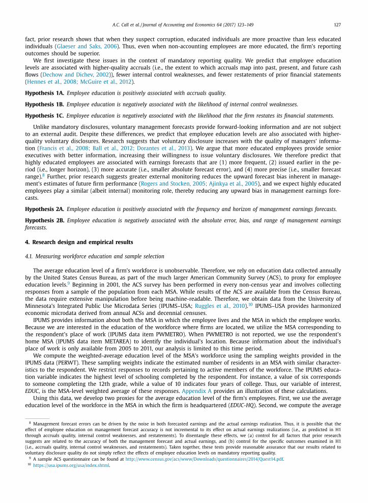
fact, prior research shows that when they suspect corruption, educated individuals are more proactive than less educated

individuals ( Glaeser and Saks, 2006 ). Thus, even when non-accounting employees are more educated, the firm’s reporting

outcomes should be superior.

We first investigate these issues in the context of mandatory reporting quality. We predict that employee education

levels are associated with higher-quality accruals (i.e., the extent to which accruals map into past, present, and future cash

flows ( Dechow and Dichev, 2002 )), fewer internal control weaknesses, and fewer restatements of prior financial statements

( Hennes et al., 2008; McGuire et al., 2012 ).

Hypothesis 1A. Employee education is positively associated with accruals quality.

Hypothesis 1B. Employee education is negatively associated with the likelihood of internal control weaknesses.

Hypothesis 1C. Employee education is negatively associated with the likelihood that the firm restates its financial statements.

Unlike mandatory disclosures, voluntary management forecasts provide forward-looking information and are not subject

to an external audit. Despite these differences, we predict that employee education levels are also associated with higher-

quality voluntary disclosures. Research suggests that voluntary disclosure increases with the quality of managers’ informa-

tion ( Francis et al., 2008; Ball et al., 2012; Dorantes et al., 2013 ). We argue that more educated employees provide senior

executives with better information, increasing their willingness to issue voluntary disclosures. We therefore predict that

highly educated employees are associated with earnings forecasts that are (1) more frequent, (2) issued earlier in the pe-

riod (i.e., longer horizon), (3) more accurate (i.e., smaller absolute forecast error), and (4) more precise (i.e., smaller forecast

range). 8 Further, prior research suggests greater external monitoring reduces the upward forecast bias inherent in manage-

ment’s estimates of future firm performance ( Rogers and Stocken, 2005; Ajinkya et al., 2005 ), and we expect highly educated

employees play a similar (albeit internal) monitoring role, thereby reducing any upward bias in management earnings fore-

casts.

Hypothesis 2A. Employee education is positively associated with the frequency and horizon of management earnings forecasts.

Hypothesis 2B. Employee education is negatively associated with the absolute error, bias, and range of management earnings

forecasts.

4. Research design and empirical results

4.1. Measuring workforce education and sample selection

The average education level of a firm’s workforce is unobservable. Therefore, we rely on education data collected annually

by the United States Census Bureau, as part of the much larger American Community Survey (ACS), to proxy for employee

education levels. 9 Beginning in 2001, the ACS survey has been performed in every non-census year and involves collecting

responses from a sample of the population from each MSA. While results of the ACS are available from the Census Bureau,

the data require extensive manipulation before being machine-readable. Therefore, we obtain data from the University of

Minnesota’s Integrated Public Use Microdata Series (IPUMS–USA; Ruggles et al., 2010 ). 10 IPUMS–USA provides harmonized

economic microdata derived from annual ACSs and decennial censuses.

IPUMS provides information about both the MSA in which the employee lives and the MSA in which the employee works.

Because we are interested in the education of the workforce where firms are located, we utilize the MSA corresponding to

the respondent’s place of work (IPUMS data item PWMETRO). When PWMETRO is not reported, we use the respondent’s

home MSA (IPUMS data item METAREA) to identify the individual’s location. Because information about the individual’s

place of work is only available from 2005 to 2011, our analysis is limited to this time period.

We compute the weighted-average education level of the MSA’s workforce using the sampling weights provided in the

IPUMS data (PERWT). These sampling weights indicate the estimated number of residents in an MSA with similar character-

istics to the respondent. We restrict responses to records pertaining to active members of the workforce. The IPUMS educa-

tion variable indicates the highest level of schooling completed by the respondent. For instance, a value of six corresponds

to someone completing the 12th grade, while a value of 10 indicates four years of college. Thus, our variable of interest,

EDUC , is the MSA-level weighted average of these responses. Appendix A provides an illustration of these calculations.

Using this data, we develop two proxies for the average education level of the firm’s employees. First, we use the average

education level of the workforce in the MSA in which the firm is headquartered ( EDUC-HQ ). Second, we compute the average

8 Management forecast errors can be driven by the noise in both forecasted earnings and the actual earnings realization. Thus, it is possible that the

effect of employee education on management forecast accuracy is not incremental to its effect on actual earnings realizations (i.e., as predicted in H1

through accruals quality, internal control weaknesses, and restatements). To disentangle these effects, we (a) control for all factors that prior research

suggests are related to the accuracy of both the management forecast and actual earnings, and (b) control for the specific outcomes examined in H1

(i.e., accruals quality, internal control weaknesses, and restatements). Taken together, these tests provide reasonable assurance that our results related to

voluntary disclosure quality do not simply reflect the effects of employee education levels on mandatory reporting quality. 9 A sample ACS questionnaire can be found at http://www.census.gov/acs/www/Downloads/questionnaires/2014/Quest14.pdf .

10 https://usa.ipums.org/usa/index.shtml .

128 A.C. Call et al. / Journal of Accounting and Economics 64 (2017) 123–149

education level of all MSAs in which the firm had significant operations during the year, acknowledging that many firms

have employees who work outside the firm’s headquarters MSA. We capture the education level of employees at other

firm locations because sales and other accounting information often originates away of headquarters. However, even if the

underlying information originates elsewhere, accounting information is often aggregated and summarized by employees at

firm headquarters. Therefore, we employ both proxies in our empirical tests and make no prediction about which proxy

better captures the quality of the employees most closely associated with reporting outcomes.

We use Compustat to identify the headquarters address, and then obtain latitude and longitude data using Google’s ‘geo-

coding’ functionality to compute the average straight-line distance between the firm’s headquarters and the center of each

city named in the description of each MSA (e.g., “Dallas” and “Fort Worth” for Dallas-Fort Worth). We assign observations to

the closest MSA using this average straight-line distance. The mean (median) distance between firm headquarters and the

center of the nearest city named in an MSA is 7.8 (0) miles, and less than 1% of observations are more than 60 miles from

the center of the closest MSA. 11 We then merge the education data based on the firm’s fiscal year end. 12

We search for locations in firms’ 10-Ks using a process similar to Bernile et al. (2015) and Garcia and Norli (2012) .

Specifically, we search for city-state locations that appear in any portion (excluding the header) of a firm’s 10-K filing. 13

We then validate each match using a comprehensive list of nearly 30,0 0 0 US cities, and map these city-state combinations

into MSAs. 14 We find substantial variation in the number of locations identified in the 10-K. For about 20% of the firm-year

observations in our sample, we find no mention in the 10-K of locations outside of the firm’s headquarters MSA. However,

for the remaining 80%, we identify multiple MSAs, and in these cases, we calculate the firm’s employee education level as

the simple average of the average education level across these MSAs ( EDUC-10K ). 15

We obtain financial data from the CRSP-Compustat merged database. Because the ACS data is limited to the population

of the United States, we delete firms headquartered outside the US. We also remove firms headquartered in Puerto Rico

because local regulations likely differ when compared to firms headquartered elsewhere in the US. This process yields 34,090

firm-year observations between 2005 and early 2012. Each of our analyses begins with this population, although additional

data requirements yield much smaller samples in our tests. We discuss these restrictions below.

In our analyses, we control for several MSA-level variables. Specifically, we control for the average wages in the MSA

( WAGES ), the natural log of the size of the workforce in the MSA ( LNPOP ), and the cost of living using the MSA’s consumer-

price index ( CPI ). We also control for the level of religious adherence ( RELIGION ), as prior research links religiosity to fi-

nancial reporting ( Dyreng et al., 2012; McGuire et al., 2012 ) and the intensity of press coverage ( REPORTERS ), since research

identifies journalists as capable monitors ( Miller, 2006 ). Further, we control for the MSA’s economic environment using un-

employment ( UNEMP ), new housing starts ( HOUSESTARTS ), the state coincident index ( SCI ), a summary measure of economic

condition, and average profitability and earnings volatility ( MSA_ROA and MSA_ROA_VOL , respectively). We compute each of

these MSA-level variables using the same two measurement bases (headquarters MSA or 10-K MSAs) described for EDUC .

We expect RELIGION to relate positively to reporting quality based on evidence in Dyreng et al. (2012) and McGuire et al.

(2012) , but we make no other predictions related to these MSA variables.

We also control for several firm-level measures associated with the firm’s geographic location and that may correlate

with employee quality. Specifically, research suggests auditors ( Choi et al., 2012 ), the SEC ( Kedia and Rajgopal, 2011 ), secu-

rity analysts ( Yu, 2008 ), and institutional ownership ( Ayers et al., 2011 ) are all associated with financial reporting quality.

Accordingly, we control for the proximity of the firm to these monitors. Specifically, we control for the natural log of the

distance between the firm’s headquarters and its auditor ( AUDITORDIST ), the responsible SEC regional office ( SECDIST ), and

New York City ( NYCDIST ), where more than half of all analysts are located ( Gunn, 2013 ). We expect each of these distance

measures to relate negatively to financial reporting quality. We also control for local institutional ownership ( LOCMONITOR )

and analyst following ( AFOLLOW ) in all analyses. 16 We expect both of these variables to relate positively to financial re-

porting quality. Finally, we control for the education level of named executives and directors ( BOARDEDUC ) using degree

information from BoardEx. Because of BoardEx’s limited coverage, we set BOARDEDUC equal to zero and include an indicator

variable ( MISSING_BX ) equal to one for observations without BoardEx data. Appendix B provides detailed definitions of all

variables.

11 Our findings are not sensitive to dropping firms with headquarters more than 60 miles from the center of the closest MSA. 12 We assume ACS data is collected throughout the year. Therefore, for firms with fiscal years prior to July 1, we use the prior year education data. For

fiscal years that end after July 1, we use the current year education data. 13 We use a Python script to identify city-state combinations as a proper noun (or multiple proper nouns) followed by a state name or abbreviation (with

or without comma separation). Bernile et al. (2015) and Garcia and Norli (2012) use a similar approach to identify unique states mentioned in the 10-K.

We identify city-state combinations, rather than states, to allow for more precise mapping into MSAs. However, to validate our approach, we also searched

for unique states and found that the firms in our sample mention an average of 8.2 unique states in the 10-K, compared to 8.1 unique states for Bernile et

al. (2015) and 7.9 unique states for Garcia and Norli (2012) . 14 See http://opengeocode.org/download.php for the list of cities. 15 In untabulated analysis, we also calculate a measure that weights each MSA by its number of mentions in the 10-K under the assumption that more fre-

quently mentioned locations have a greater proportion of firm operations. Results using this alternative measure are qualitatively similar to those reported

in our analyses using the simple average. 16 As in Ayers et al. (2011) , we also control for other classifications of institutional ownership (i.e., non-local monitors, transient owners, and other

owners).

A.C. Call et al. / Journal of Accounting and Economics 64 (2017) 123–149 129

4.2. Descriptive statistics for MSA data

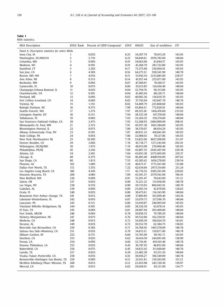
Table 1 presents descriptive statistics for our MSA-level variables. In Panel A, we sort MSAs by mean education, where

lower (higher) ranks correspond to a more (less) educated workforce. We report descriptive statistics for the 25 MSAs with

the highest and lowest values of EDUC , along with any MSA that are headquarters to at least 1% of observations in the CRSP-

Compustat universe during our sample period. A score of 7 (8) corresponds to one (two) years of college completed, and the

education level corresponding to each value of EDUC is outlined in Appendix B . The most educated cities often correspond

to “college towns” (e.g., Iowa City, Ann Arbor, Gainesville), although a few larger cities appear in this list of the 25 most

educated MSAs as well (e.g., Boston, New York). The 25 MSAs with the lowest education levels represent areas typically

associated with economic hardship and high poverty levels (e.g., Stockton, Modesto). Panel A also reports average WAGES ,

the average size of the workforce, and the average CPI for each MSA during our sample period. As expected, larger cities

typically correspond to higher cost of living and wages. However, wages can also be associated with education, highlighting

the importance of controlling for these potentially confounding factors.

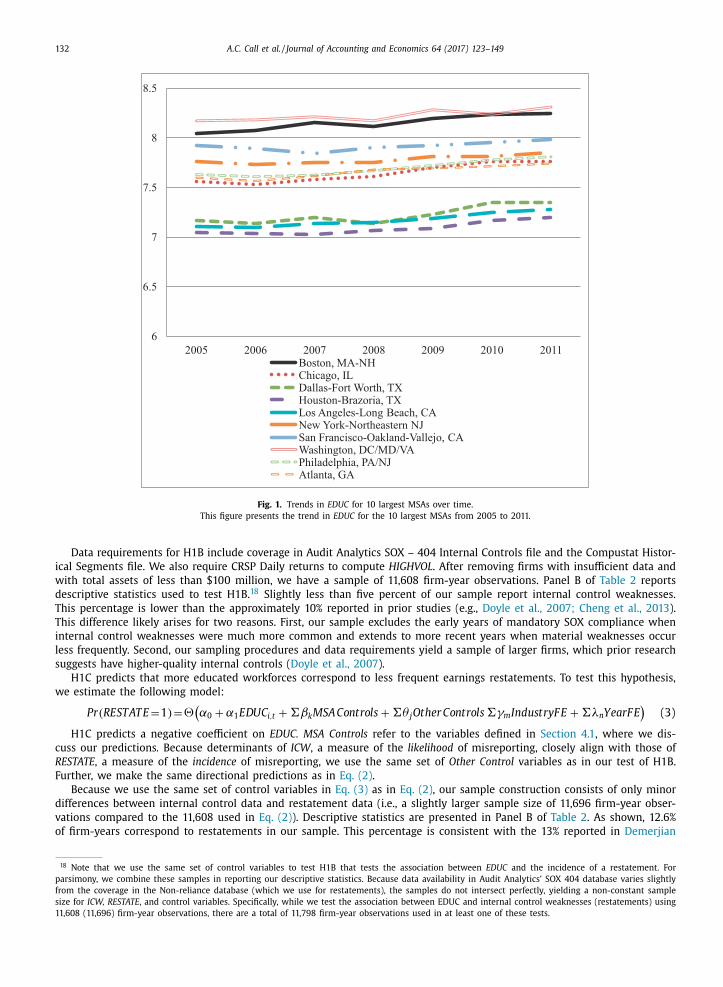
Panel B of Table 1 reports descriptive statistics for select MSA-level variables separately for each year. Average EDUC ex-

hibits a modest increase over our sample period, increasing from 7.31 in 2005 to 7.47 in 2011. For context, one scenario that

could lead to this increase of 0.16 is for 16% of the workforce to complete one additional year of college. To further inves-

tigate the time-series properties of EDUC , Fig. 1 plots EDUC values for the largest ten MSAs from 2005 to 2011. Consistent

with Panel B of Table 1 , education is increasing over time. However, there is MSA-level variation regarding the magnitude

of this increase over our sample period.

In Panel C of Table 1 , we sort MSAs into deciles by EDUC , where Decile 1 corresponds to the most educated locations.

We then present the mean value of EDUC , along with the number and percentage of observations in our sample, within

each decile. A large proportion of observations correspond to firms located in more educated cities, as approximately 60% of

observations fall within the first three education deciles. However, nearly 17% of observations fall within the bottom three

deciles. Panel D of Table 1 presents correlations among MSA variables. EDUC exhibits significant correlations with all MSA

variables. Specifically, EDUC correlates positively with WAGES , LN_POP, CPI, HOUSESTARTS, REPORTERS, and MSA_ROA_VOL ,

with correlations ranging from 0.12 to 0.39. EDUC correlates negatively with UNEMP, RELIGION, SCI, and MSA_ROA , with

correlations ranging from −0.12 to −0.21. We control for these variables in all regressions.

4.3. Research design for H1

H1A predicts that larger values of EDUC ( EDUC-HQ and EDUC-10K ) are associated with higher-quality accruals. Using a

modified Dechow–Dichev measure of accruals quality ( AQ ) ( Dechow and Dichev, 2002; McNichols, 2002 ), we estimate the

following regression (with firm and year subscripts i and t ):

A Q i,t = α0 + α1 EDU C i,t + �βk MSA Controls + �θ j Other Controls + �γm

Industr yF E + �λn Year F E + e i,t (1)

We estimate Eq. (1) using OLS, and assess statistical significance throughout the paper using one- (two-) sided p -values

when predictions are (are not) made using t -statistics derived from robust standard errors clustered by firm. Because smaller

values of AQ correspond to better accruals quality, we expect α1 to be negative. MSA Controls refer to those variables defined

in Section 4.1 (i.e., WAGES, RELIGION, NYDIST, etc.), and are included in all regressions.

The remaining control variables ( Other Controls ) are largely based on Francis et al. (2004) . We expect AQ to deteriorate

(or increase in magnitude) with increases in the volatility of fundamentals ( SALEVOL and CFVOL ) , the length of the operating

cycle ( LNOPCYCLE ) , the intensity of intangible assets ( INT_INT ) and the incidence of negative earnings ( NLOSSES ), because

higher values of these firm characteristics make accrual estimation more difficult. Conversely, larger firms ( LNASSETS ), firms

with more capital assets ( CAP_INT ), and those audited by a Big 4 auditor ( BIG4 ) typically exhibit higher accruals quality. In

addition to these measures, we also include firm and peer idiosyncratic shocks ( IDIOSHOCKS and PEERSHOCKS ) derived from

returns data based on evidence in Owens et al. (2017) . We expect each of these measures to relate positively to AQ . We

remove firms with less than $100 million in assets to avoid small denominator problems. Many variables ( CFVOL, SALEVOL,

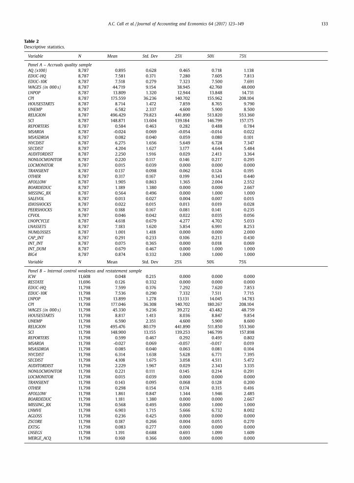
NLOSSES ) require a five-year time series to calculate. These screens result in a sample of 8,787 firm-year observations. De-

scriptive statistics for this sample are presented in Panel A of Table 2. 17 Appendix B presents detailed definitions of all

variables.

H1B uses the effectiveness of internal controls over financial reporting ( Feng et al., 2009 ) to proxy for the quality of

the firm’s mandatory disclosures. Better internal controls decrease the likelihood that errors or irregularities go undetected.

Thus, we estimate the following regression:

P r ( IC W i,t = 1 ) = (α0 + α1 EDU C i,t + +�βk MSA Controls + �θ j Other Controls �γm

Industr yF E + �λn Year F E )

( 2)

where (.) is the logistic function and ICW i,t is equal to one if firm i has an internal control weakness in year t , and zero

otherwise.

17 We winsorize all continuous, unlogged variables at the top and bottom one percent. The descriptive statistics in Panel A of Table 2 are largely consistent

with those found in prior research.

130 A.C. Call et al. / Journal of Accounting and Economics 64 (2017) 123–149

Table 1

MSA statistics.

MSA Description EDUC Rank Percent of CRSP-Compustat a EDUC WAGES Size of workforce CPI

Panel A: Descriptive statistics for select MSAs

Iowa City, IA 1 0 .03% 8 .25 34,307 .79 70,913 .29 143 .95

Washington, DC/MD/VA 2 2 .73% 8 .22 58,849 .61 2976,782 .00 140 .84

Columbia, MO 3 0 .06% 8 .19 34,063 .06 81,844 .57 143 .95

Madison, WI 4 0 .19% 8 .19 41,268 .79 281,722 .80 143 .95

Stamford, CT 5 2 .26% 8 .17 73,375 .68 210,004 .10 145 .03

San Jose, CA 6 4 .58% 8 .16 64,273 .12 938,541 .90 140 .78

Boston, MA–NH 7 4 .93% 8 .15 51,945 .54 2213,885 .00 228 .57

Ann Arbor, MI 8 0 .31% 8 .14 41,957 .44 255,071 .00 143 .95

Rochester, MN 9 0 .09% 8 .07 47,560 .97 76,169 .57 143 .95

Gainesville, FL 10 0 .07% 8 .06 35,613 .85 114,436 .40 140 .84

Champaign-Urbana-Rantoul, IL 11 0 .02% 8 .04 32,794 .76 96,313 .86 143 .95

Charlottesville, VA 12 0 .10% 8 .04 41,405 .94 88,120 .71 140 .84

Portland, ME 13 0 .09% 8 .03 40,092 .36 136,819 .70 145 .03

Fort Collins–Loveland, CO 14 0 .06% 8 .02 37,792 .04 143,847 .70 140 .78

Trenton, NJ 15 1 .15% 8 .02 54,489 .79 225,868 .60 145 .03

Raleigh–Durham, NC 16 0 .57% 7 .99 43,864 .13 772,820 .10 140 .84

Seattle–Everett, WA 17 1 .27% 7 .97 49,525 .18 1418,476 .00 233 .92

Lexington–Fayette, KY 18 0 .11% 7 .94 38,325 .38 147,376 .00 140 .84

Tallahassee, FL 19 0 .06% 7 .93 35,264 .35 150,274 .60 140 .84

San Francisco–Oakland–Vallejo, CA 20 2 .47% 7 .92 52,268 .93 2404,900 .00 208 .10

Minneapolis–St. Paul, MN 21 2 .31% 7 .91 45,957 .38 1661,384 .00 143 .95

Bloomington–Normal, IL 22 0 .07% 7 .89 38,370 .07 88,654 .29 143 .95

Albany–Schenectady–Troy, NY 23 0 .19% 7 .87 40,831 .32 418,841 .00 145 .03

State College, PA 24 0 .05% 7 .86 32,908 .63 70,127 .86 145 .03

New York–Northeastern NJ 25 10 .30% 7 .78 53,822 .96 8627,209 .00 211 .67

Denver–Boulder, CO 29 2 .06% 7 .76 43,718 .77 1271,245 .00 202 .10

Wilmington, DE/NJ/MD 36 1 .97% 7 .74 49,013 .09 270,906 .40 145 .03

Philadelphia, PA/NJ 45 2 .24% 7 .69 45,807 .35 24 45,4 47 .00 220 .38

Atlanta, GA 54 2 .16% 7 .66 43,855 .38 2375,605 .00 210 .37

Chicago, IL 60 6 .37% 7 .64 46,405 .40 4408,916 .00 207 .62

San Diego, CA 80 1 .81% 7 .55 43,505 .62 1456,278 .00 230 .54

Phoenix, AZ 165 1 .08% 7 .24 40,673 .17 1775,561 .00 132 .88

Dallas–Fort Worth, TX 172 3 .35% 7 .22 42,634 .66 2973,514 .00 211 .24

Los Angeles–Long Beach, CA 186 4 .34% 7 .17 42,776 .35 6185,291 .00 220 .02

Houston–Brazoria, TX 206 4 .08% 7 .09 43,501 .37 2579,541 .00 196 .10

New Bedford, MA 236 0 .00% 6 .91 33,201 .47 70,643 .00 131 .12

Salem, OR 237 0 .02% 6 .90 31,221 .22 131,958 .90 140 .78

Las Vegas, NV 238 0 .55% 6 .90 39,733 .03 884,943 .10 140 .78

Gadsden, AL 239 0 .00% 6 .89 25,692 .54 42,870 .00 128 .63

Ocala, FL 240 0 .02% 6 .88 30,473 .61 114,343 .90 140 .84

Beaumont–Port Arthur–Orange, TX 241 0 .01% 6 .88 37,869 .89 163,699 .40 144 .36

Lakeland–Winterhaven, FL 242 0 .05% 6 .87 33,079 .73 217,596 .70 140 .84

Lancaster, PA 243 0 .11% 6 .86 33,659 .87 240,095 .00 145 .03

Vineland–Milville–Bridgetown, NJ 244 0 .10% 6 .85 38,326 .39 63,678 .14 145 .03

El Paso, TX 245 0 .06% 6 .81 28,807 .94 303,409 .60 140 .84

Fort Smith, AR/OK 246 0 .06% 6 .78 30,858 .35 79,789 .29 140 .84

Hickory–Morgantown, NC 247 0 .07% 6 .76 30,532 .06 162,250 .10 140 .84

Modesto, CA 248 0 .01% 6 .72 34,450 .39 184,624 .70 143 .81

Decatur, AL 249 0 .02% 6 .72 30,552 .70 62,384 .75 138 .83

Riverside–San Bernardino, CA 250 0 .38% 6 .71 34,766 .95 1491,578 .00 140 .78

Salinas–Sea Side–Monterey, CA 251 0 .03% 6 .70 34,813 .15 120,877 .60 140 .78

Elkhart–Goshen, IN 252 0 .17% 6 .66 33,765 .99 99,741 .71 143 .95

Stockton, CA 253 0 .02% 6 .62 34,414 .50 244,691 .00 138 .90

Fresno, CA 254 0 .09% 6 .60 32,756 .18 419,165 .40 140 .78

Houma–Thibodoux, LA 255 0 .02% 6 .45 36,747 .92 48,852 .00 140 .84

Bakersfield, CA 256 0 .07% 6 .45 34,833 .42 311,660 .80 140 .78

Laredo, TX 257 0 .02% 6 .28 25,402 .30 93,251 .29 140 .84

Visalia–Tulare–Porterville, CA 258 0 .03% 6 .16 30,036 .27 160,349 .00 140 .78

Brownsville–Harlingen–San Benito, TX 259 0 .00% 6 .15 25,611 .81 139,303 .00 151 .13

McAllen–Edinburg–Pharr–Mission, TX 260 0 .01% 6 .12 23,453 .98 243,720 .30 139 .97

Merced, CA 261 0 .01% 6 .02 29,028 .91 85,121 .00 134 .77

A.C. Call et al. / Journal of Accounting and Economics 64 (2017) 123–149 131

Table 1

( continued )

ACS year EDUC WAGES Size of workforce CPI

Panel B: Descriptive statistics for MSA variables by year

2005 7.31 34,241 .64 410,158 .00 136 .05

2006 7.31 34,944 .70 429,656 .88 143 .27

2007 7.34 36,543 .42 430,614 .91 148 .57

2008 7.36 37,552 .45 447,073 .09 159 .60

2009 7.42 38,045 .14 435,437 .28 147 .82

2010 7.45 37,997 .47 431,735 .56 148 .68

2011 7.47 38,4 4 4 .71 436,804 .50 159 .02

Total 7.38 36,951 .07 429,869 .10 148 .93

Decile EDUC Observations Percentage Cumulative Percentage

Panel C: CRSP/Compustat observations by EDUC decile

1 8.04 8,346 24 .48% 24 .48%

2 7.73 7,602 22 .30% 46 .78%

3 7.63 5,203 15 .26% 62 .04%

4 7.52 2,386 7 .00% 69 .04%

5 7.43 1,488 4 .36% 73 .41%

6 7.34 1,437 4 .22% 77 .62%

7 7.24 1,849 5 .42% 83 .05%

8 7.15 3,702 10 .86% 93 .91%

9 7.02 1,374 4 .03% 97 .94%

10 6.69 703 2 .06% 100 .00%

(1) (2) (3) (4) (5) (6) (7) (8) (9) (10) (11)

Panel D: Correlations among MSA-level measures

(1) EDUC 0 .558 0 .292 0 .237 0 .189 −0 .098 −0 .140 −0 .106 0 .254 −0 .161 0 .202

(2) WAGES 0 .386 0 .578 0 .400 0 .393 0 .053 −0 .060 −0 .019 0 .200 −0 .267 0 .455

(3) LNPOP 0 .136 0 .085 0 .210 0 .723 −0 .004 −0 .079 0 .110 0 .271 −0 .189 0 .389

(4) CPI 0 .237 0 .393 0 .527 −0 .065 0 .254 −0 .016 −0 .136 0 .083 −0 .111 0 .219

(5) HOUSESTARTS 0 .170 0 .346 0 .710 0 .242 −0 .309 −0 .083 0 .326 0 .177 −0 .103 0 .277

(6) UNEMP −0 .213 −0 .013 −0 .043 0 .070 −0 .308 −0 .102 −0 .274 −0 .084 −0 .057 0 .068

(7) RELIGION −0 .180 −0 .127 0 .064 −0 .045 −0 .112 −0 .141 −0 .129 −0 .055 0 .160 −0 .060

(8) SCI −0 .136 −0 .024 0 .058 −0 .091 0 .291 −0 .167 −0 .149 −0 .007 −0 .082 0 .130

(9) REPORTERS 0 .118 0 .007 0 .031 0 .012 0 .008 −0 .078 0 .007 −0 .012 −0 .069 0 .111

(10) MSA_ROA −0 .123 −0 .199 −0 .155 −0 .128 −0 .111 −0 .010 0 .141 −0 .085 0 .049 −0 .369

(11) MSA_ROA_VOL 0 .124 0 .270 0 .280 0 .199 0 .215 0 .024 −0 .027 0 .165 −0 .001 −0 .412

Panel A of Table 1 presents average MSA-level descriptive statistics over our sample period for a selection of locations where at least one firm in CRSP-

Compustat database is headquartered. We rank cities by average education level and present the top 25, bottom 25, and cities with at least 1% of observa-

tions in CRSP-Compustat between 2005 and 2011. Lower (higher) EDUC ranks correspond to more (less) educated MSAs.

Panel B of Table 1 presents average MSA-level statistics by year.

Panel C of Table 1 presents the distribution of CRSP-Compustat observations by EDUC decile as well as average EDUC for MSAs in each decile. Lower (higher)

ranks correspond to more (less) educated MSAs.

Panel D of Table 1 presents correlations between variables of interest and EDUC . Pearson (Spearman) correlations are reported below (above) the diagonal.

Italicized correlations are insignificantly different from 0 ( p > 0.05).

All variables are defined in Appendix B . a The percentage of firms in each MSA in the CRSP-Compustat universe is correlated with the percentage of firms in each MSA for each our samples

throughout the paper at Pearson Correlations greater than 90% ( ρ ≥ 0.90). Thus, for brevity, we only report the percentage for the entire CRSP-Compustat

universe.

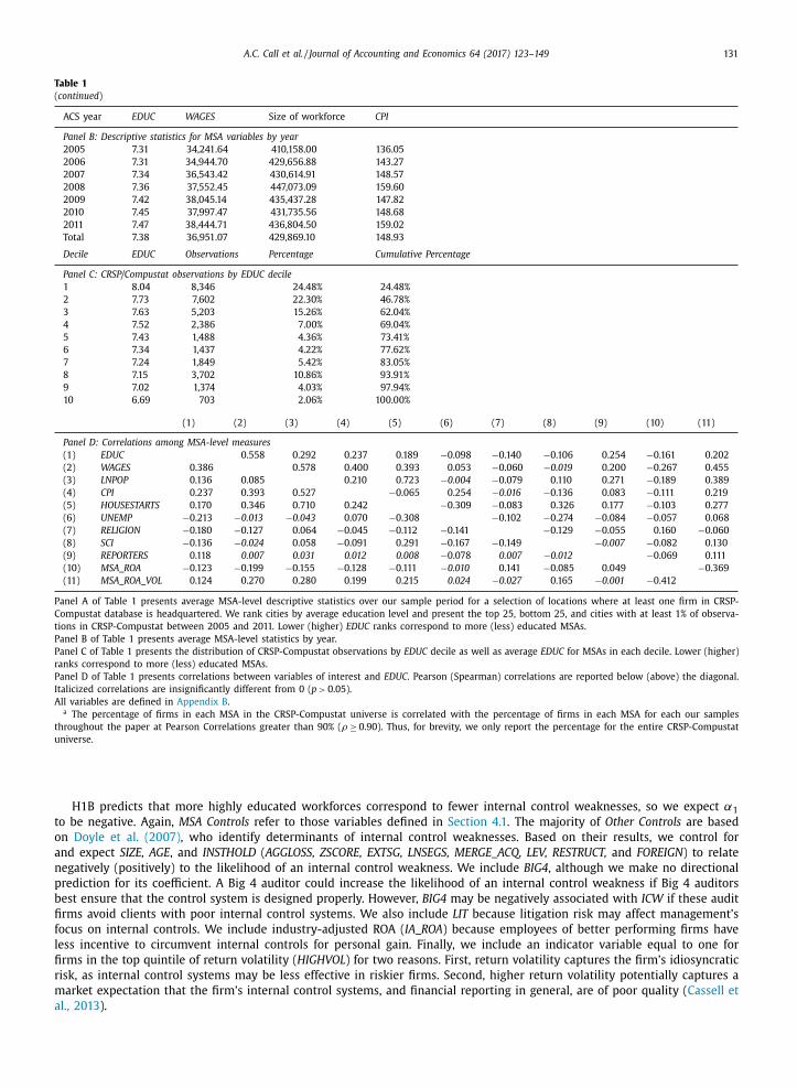
H1B predicts that more highly educated workforces correspond to fewer internal control weaknesses, so we expect α1

to be negative. Again, MSA Controls refer to those variables defined in Section 4.1 . The majority of Other Controls are based

on Doyle et al. (2007) , who identify determinants of internal control weaknesses. Based on their results, we control for

and expect SIZE, AGE , and INSTHOLD ( AGGLOSS, ZSCORE, EXTSG, LNSEGS, MERGE_ACQ, LEV, RESTRUCT, and FOREIGN ) to relate

negatively (positively) to the likelihood of an internal control weakness. We include BIG4 , although we make no directional

prediction for its coefficient. A Big 4 auditor could increase the likelihood of an internal control weakness if Big 4 auditors

best ensure that the control system is designed properly. However, BIG4 may be negatively associated with ICW if these audit

firms avoid clients with poor internal control systems. We also include LIT because litigation risk may affect management’s

focus on internal controls. We include industry-adjusted ROA ( IA_ROA ) because employees of better performing firms have

less incentive to circumvent internal controls for personal gain. Finally, we include an indicator variable equal to one for

firms in the top quintile of return volatility ( HIGHVOL ) for two reasons. First, return volatility captures the firm’s idiosyncratic

risk, as internal control systems may be less effective in riskier firms. Second, higher return volatility potentially captures a

market expectation that the firm’s internal control systems, and financial reporting in general, are of poor quality ( Cassell et

al., 2013 ).

132 A.C. Call et al. / Journal of Accounting and Economics 64 (2017) 123–149

6

6.5

7

7.5

8

8.5

2005 2006 2007 2008 2009 2010 2011Boston, MA-NHChicago, ILDallas-Fort Worth, TXHouston-Brazoria, TXLos Angeles-Long Beach, CANew York-Northeastern NJSan Francisco-Oakland-Vallejo, CAWashington, DC/MD/VAPhiladelphia, PA/NJAtlanta, GA

Fig. 1. Trends in EDUC for 10 largest MSAs over time.

This figure presents the trend in EDUC for the 10 largest MSAs from 2005 to 2011.

Data requirements for H1B include coverage in Audit Analytics SOX – 404 Internal Controls file and the Compustat Histor-

ical Segments file. We also require CRSP Daily returns to compute HIGHVOL . After removing firms with insufficient data and

with total assets of less than $100 million, we have a sample of 11,608 firm-year observations. Panel B of Table 2 reports

descriptive statistics used to test H1B. 18 Slightly less than five percent of our sample report internal control weaknesses.

This percentage is lower than the approximately 10% reported in prior studies (e.g., Doyle et al., 2007; Cheng et al., 2013 ).

This difference likely arises for two reasons. First, our sample excludes the early years of mandatory SOX compliance when

internal control weaknesses were much more common and extends to more recent years when material weaknesses occur

less frequently. Second, our sampling procedures and data requirements yield a sample of larger firms, which prior research

suggests have higher-quality internal controls ( Doyle et al., 2007 ).

H1C predicts that more educated workforces correspond to less frequent earnings restatements. To test this hypothesis,

we estimate the following model:

P r ( REST AT E =1 ) =(α0 + α1 EDU C i,t + �βk MSA Controls + �θ j Other Controls �γm

Industr yF E + �λn Year F E )

(3)

H1C predicts a negative coefficient on EDUC. MSA Controls refer to the variables defined in Section 4.1 , where we dis-

cuss our predictions . Because determinants of ICW , a measure of the likelihood of misreporting, closely align with those of

RESTATE , a measure of the incidence of misreporting, we use the same set of Other Control variables as in our test of H1B.

Further, we make the same directional predictions as in Eq. (2) .

Because we use the same set of control variables in Eq. (3) as in Eq. (2) , our sample construction consists of only minor

differences between internal control data and restatement data (i.e., a slightly larger sample size of 11,696 firm-year obser-

vations compared to the 11,608 used in Eq. (2) ). Descriptive statistics are presented in Panel B of Table 2 . As shown, 12.6%

of firm-years correspond to restatements in our sample. This percentage is consistent with the 13% reported in Demerjian

18 Note that we use the same set of control variables to test H1B that tests the association between EDUC and the incidence of a restatement. For

parsimony, we combine these samples in reporting our descriptive statistics. Because data availability in Audit Analytics’ SOX 404 database varies slightly

from the coverage in the Non-reliance database (which we use for restatements), the samples do not intersect perfectly, yielding a non-constant sample

size for ICW, RESTATE , and control variables. Specifically, while we test the association between EDUC and internal control weaknesses (restatements) using

11,608 (11,696) firm-year observations, there are a total of 11,798 firm-year observations used in at least one of these tests.

A.C. Call et al. / Journal of Accounting and Economics 64 (2017) 123–149 133

Table 2

Descriptive statistics.

Variable N Mean Std . Dev 25% 50% 75%

Panel A – Accruals quality sample

AQ (x100) 8,787 0 .895 0 .628 0 .465 0 .718 1 .138

EDUC-HQ 8,787 7 .581 0 .371 7 .280 7 .605 7 .813

EDUC-10K 8,787 7 .518 0 .279 7 .323 7 .500 7 .691

WAGES (in 0 0 0 s) 8,787 44 .719 9 .154 38 .945 42 .760 48 .0 0 0

LNPOP 8,787 13 .809 1 .320 12 .944 13 .848 14 .731

CPI 8,787 175 .559 36 .236 140 .702 155 .962 208 .104

HOUSESTARTS 8,787 8 .714 1 .472 7 .859 8 .765 9 .790

UNEMP 8,787 6 .582 2 .337 4 .600 5 .900 8 .500

RELIGION 8,787 496 .429 79 .823 441 .890 513 .820 553 .360

SCI 8,787 148 .871 13 .604 139 .184 146 .799 157 .175

REPORTERS 8,787 0 .584 0 .463 0 .282 0 .488 0 .784

MSAROA 8,787 -0 .024 0 .069 -0 .054 -0 .014 0 .022

MSASDROA 8,787 0 .082 0 .040 0 .059 0 .080 0 .101

NYCDIST 8,787 6 .275 1 .656 5 .649 6 .728 7 .347

SECDIST 8,787 4 .204 1 .627 3 .177 4 .644 5 .484

AUDITORDIST 8,787 2 .250 1 .916 0 .029 2 .413 3 .364

NONLOCMONITOR 8,787 0 .220 0 .117 0 .146 0 .217 0 .295

LOCMONITOR 8,787 0 .015 0 .039 0 .0 0 0 0 .0 0 0 0 .0 0 0

TRANSIENT 8,787 0 .137 0 .098 0 .062 0 .124 0 .195

OTHER 8,787 0 .317 0 .167 0 .199 0 .343 0 .440

AFOLLOW 8,787 1 .905 0 .863 1 .365 2 .004 2 .552

BOARDEDUC 8,787 1 .189 1 .380 0 .0 0 0 0 .0 0 0 2 .667

MISSING_BX 8,787 0 .564 0 .496 0 .0 0 0 1 .0 0 0 1 .0 0 0

SALEVOL 8,787 0 .013 0 .027 0 .004 0 .007 0 .015

IDIOSHOCKS 8,787 0 .022 0 .015 0 .013 0 .019 0 .028

PEERSHOCKS 8,787 0 .188 0 .167 0 .081 0 .141 0 .235

CFVOL 8,787 0 .046 0 .042 0 .022 0 .035 0 .056

LNOPCYCLE 8,787 4 .618 0 .679 4 .277 4 .702 5 .033

LNASSETS 8,787 7 .183 1 .620 5 .854 6 .991 8 .253

NUMLOSSES 8,787 1 .001 1 .418 0 .0 0 0 0 .0 0 0 2 .0 0 0

CAP_INT 8,787 0 .291 0 .233 0 .106 0 .213 0 .430

INT_INT 8,787 0 .075 0 .365 0 .0 0 0 0 .018 0 .069

INT_DUM 8,787 0 .679 0 .467 0 .0 0 0 1 .0 0 0 1 .0 0 0

BIG4 8,787 0 .874 0 .332 1 .0 0 0 1 .0 0 0 1 .0 0 0

Variable N Mean Std . Dev 25% 50% 75%

Panel B – Internal control weakness and restatement sample

ICW 11,608 0 .048 0 .215 0 .0 0 0 0 .0 0 0 0 .0 0 0

RESTATE 11,696 0 .126 0 .332 0 .0 0 0 0 .0 0 0 0 .0 0 0

EDUC-HQ 11,798 7 .599 0 .376 7 .292 7 .620 7 .853

EDUC-10K 11,798 7 .536 0 .290 7 .332 7 .511 7 .715

LNPOP 11,798 13 .899 1 .278 13 .131 14 .045 14 .783

CPI 11,798 177 .046 36 .308 140 .702 180 .267 208 .104

WAGES (in 0 0 0 s) 11,798 45 .330 9 .236 39 .272 43 .482 48 .759

HOUSESTARTS 11,798 8 .817 1 .413 8 .036 8 .847 9 .854

UNEMP 11,798 6 .590 2 .351 4 .600 5 .900 8 .600

RELIGION 11,798 495 .476 80 .179 441 .890 511 .850 553 .360

SCI 11,798 148 .900 13 .155 139 .253 146 .799 157 .898

REPORTERS 11,798 0 .599 0 .467 0 .292 0 .495 0 .802

MSAROA 11,798 -0 .027 0 .069 -0 .057 -0 .017 0 .019

MSASDROA 11,798 0 .085 0 .040 0 .063 0 .081 0 .104

NYCDIST 11,798 6 .314 1 .638 5 .628 6 .771 7 .395

SECDIST 11,798 4 .108 1 .675 3 .058 4 .511 5 .472

AUDITORDIST 11,798 2 .229 1 .967 0 .029 2 .343 3 .335

NONLOCMONITOR 11,798 0 .221 0 .111 0 .145 0 .214 0 .291

LOCMONITOR 11,798 0 .015 0 .039 0 .0 0 0 0 .0 0 0 0 .0 0 0

TRANSIENT 11,798 0 .143 0 .095 0 .068 0 .128 0 .200

OTHER 11,798 0 .298 0 .154 0 .174 0 .315 0 .416

AFOLLOW 11,798 1 .861 0 .847 1 .344 1 .946 2 .485

BOARDEDUC 11,798 1 .181 1 .380 0 .0 0 0 0 .0 0 0 2 .667

MISSING_BX 11,798 0 .568 0 .495 0 .0 0 0 1 .0 0 0 1 .0 0 0

LNMVE 11,798 6 .903 1 .715 5 .666 6 .732 8 .002

AGLOSS 11,798 0 .236 0 .425 0 .0 0 0 0 .0 0 0 0 .0 0 0

ZSCORE 11,798 0 .187 0 .266 0 .004 0 .055 0 .270

EXTSG 11,798 0 .083 0 .277 0 .0 0 0 0 .0 0 0 0 .0 0 0

LNSEGS 11,798 1 .191 0 .688 0 .693 1 .099 1 .609

MERGE_ACQ 11,798 0 .160 0 .366 0 .0 0 0 0 .0 0 0 0 .0 0 0

134 A.C. Call et al. / Journal of Accounting and Economics 64 (2017) 123–149

Table 2

( continued )

LEV 11,798 0 .204 0 .197 0 .011 0 .174 0 .318

AGE 11,798 2 .744 0 .866 2 .215 2 .768 3 .390

RESTRUCT 11,798 0 .333 0 .471 0 .0 0 0 0 .0 0 0 1 .0 0 0

FOREIGN 11,798 0 .320 0 .467 0 .0 0 0 0 .0 0 0 1 .0 0 0

IA_ROA (unranked) 11,798 0 .046 0 .162 -0 .013 0 .035 0 .099

BIG4 11,798 0 .855 0 .352 1 .0 0 0 1 .0 0 0 1 .0 0 0

HIGHVOL 11,798 0 .215 0 .411 0 .0 0 0 0 .0 0 0 0 .0 0 0

LIT 11,798 0 .313 0 .464 0 .0 0 0 0 .0 0 0 1 .0 0 0

Variable N Mean Std . Dev 25% 50% 75%

Panel C – Management forecast sample

FREQ 5,055 2 .228 2 .394 0 .0 0 0 2 .0 0 0 4 .0 0 0

HORIZON 3,434 308 .133 121 .338 248 .0 0 0 322 .0 0 0 342 .0 0 0

ERROR 3,335 0 .010 0 .014 0 .003 0 .005 0 .010

BIAS 3,335 0 .004 0 .014 -0 .002 0 .003 0 .008

RANGE 3,015 0 .087 0 .109 0 .035 0 .057 0 .095

EDUC-HQ 5,055 7 .587 0 .371 7 .297 7 .607 7 .822

EDUC-10K 5,055 7 .523 0 .283 7 .328 7 .499 7 .699

LNPOP 5,055 13 .841 1 .295 13 .011 13 .903 14 .724

CPI 5,055 175 .098 36 .235 140 .372 155 .962 208 .104

WAGES (in 0 0 0 s) 5,055 44 .508 9 .082 38 .746 42 .668 48 .279

HOUSESTARTS 5,055 8 .852 1 .459 8 .036 8 .873 9 .911

UNEMP 5,055 6 .204 2 .226 4 .500 5 .300 7 .800

RELIGION 5,055 496 .532 79 .066 441 .890 512 .820 553 .360

SCI 5,055 148 .490 13 .080 139 .253 146 .799 153 .520

REPORTERS 5,055 0 .619 0 .479 0 .294 0 .509 0 .881

MSAROA 5,036 −0 .025 0 .071 −0 .054 −0 .017 0 .022

MSASDROA 5,030 0 .081 0 .041 0 .054 0 .081 0 .100

NYCDIST 5,055 6 .207 1 .653 5 .350 6 .637 7 .257

SECDIST 5,055 4 .181 1 .663 3 .102 4 .725 5 .523

AUDITORDIST 5,055 2 .178 1 .916 0 .029 2 .312 3 .318

NONLOCMONITOR 5,055 0 .237 0 .098 0 .168 0 .229 0 .299

LOCMONITOR 5,055 0 .015 0 .038 0 .0 0 0 0 .0 0 0 0 .0 0 0

TRANSIENT 5,055 0 .151 0 .091 0 .080 0 .136 0 .201

OTHER 5,055 0 .376 0 .134 0 .294 0 .388 0 .468

AFOLLOW 5,055 2 .130 0 .713 1 .705 2 .197 2 .657

BOARDEDUC 5,055 1 .318 1 .392 0 .0 0 0 0 .0 0 0 2 .750

MISSING_BX 5,055 0 .517 0 .500 0 .0 0 0 1 .0 0 0 1 .0 0 0

LNMVE 5,055 7 .518 1 .544 6 .399 7 .396 8 .508

BTM 5,055 0 .467 0 .298 0 .265 0 .410 0 .611

LEV 5,055 0 .205 0 .187 0 .043 0 .186 0 .307

RETVOL 5,055 0 .020 0 .010 0 .014 0 .019 0 .025

BETA 5,055 1 .136 0 .465 0 .799 1 .079 1 .414

MEANTURN 5,055 0 .010 0 .006 0 .005 0 .008 0 .012

BIG4 5,055 0 .910 0 .287 1 .0 0 0 1 .0 0 0 1 .0 0 0

LIT 5,055 0 .321 0 .467 0 .0 0 0 0 .0 0 0 1 .0 0 0

�EARN 5,055 0 .005 0 .073 −0 .012 0 .007 0 .026

LOSS 5,055 0 .139 0 .346 0 .0 0 0 0 .0 0 0 0 .0 0 0

EARNVOL 5,055 0 .041 0 .053 0 .013 0 .023 0 .043

DISPERSION 5,055 0 .040 0 .055 0 .010 0 .020 0 .040

SURPRISE 3,335 0 .003 0 .006 0 .001 0 .001 0 .004

EDUC-HQ EDUC-10K AQ ICW RESTATE FREQ HORIZON ERROR BIAS RANGE

Panel D – Correlations among dependent variables of interest and EDUC

EDUC-HQ 0 .768 −0 .003 −0 .021 −0 .012 0 .042 0 .016 −0 .043 −0 .040 −0 .063

EDUC-10K 0 .772 0 .027 −0 .017 0 .0 0 0 0 .017 −0 .047 −0 .001 −0 .031 −0 .030

AQ −0 .012 0 .024 0 .096 0 .071 −0 .169 −0 .101 0 .172 0 .075 0 .093

ICW −0 .019 −0 .014 0 .102 0 .259 −0 .073 −0 .034 0 .090 0 .061 0 .076

RESTATE −0 .012 −0 .001 0 .075 0 .259 −0 .053 −0 .034 0 .051 0 .043 0 .054

FREQ 0 .029 −0 .001 −0 .139 −0 .071 -0 .056 0 .548 0 .076 0 .187 −0 .018

HORIZON 0 .008 −0 .036 −0 .070 −0 .015 −0 .020 0 .544 0 .181 0 .378 0 .016

ERROR −0 .047 -0 .003 0 .145 0 .101 0 .020 -0 .013 0 .138 0 .401 0 .329

BIAS −0 .061 −0 .041 0 .068 0 .071 0 .037 0 .084 0 .265 0 .341 0 .002

RANGE −0 .031 0 .006 0 .103 0 .076 0 .034 −0 .088 −0 .009 0 .382 0 .118

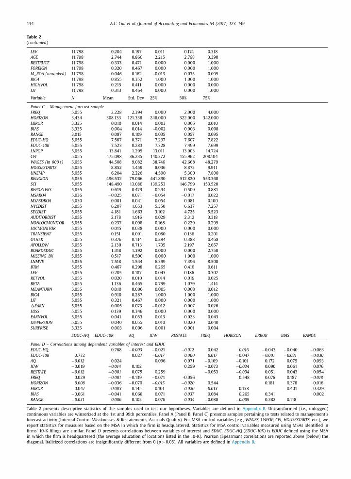
Table 2 presents descriptive statistics of the samples used to test our hypotheses. Variables are defined in Appendix B . Untransformed (i.e., unlogged)

continuous variables are winsorized at the 1st and 99th percentiles. Panel A (Panel B, Panel C) presents samples pertaining to tests related to management’s

forecast activity (Internal Control Weaknesses & Restatements, Accruals Quality). For MSA control variables (e.g., WAGES, LN POP, CPI, HOUSESTARTS, etc.), we

report statistics for measures based on the MSA in which the firm is headquartered. Statistics for MSA control variables measured using MSAs identified in

firms’ 10-K filings are similar. Panel D presents correlations between variables of interest and EDUC. EDUC-HQ ( EDUC-10K ) is EDUC defined using the MSA

in which the firm is headquartered (the average education of locations listed in the 10-K). Pearson (Spearman) correlations are reported above (below) the

diagonal. Italicized correlations are insignificantly different from 0 ( p > 0.05). All variables are defined in Appendix B .

A.C. Call et al. / Journal of Accounting and Economics 64 (2017) 123–149 135

Table 3

Relation between education and accruals quality.

AQ AQ

EDUC-HQ EDUC-10K

VARIABLES Pre dicted sign Coef. p-value Coef. p-value

MSA-year variables:

EDUC – −0 .090 ∗∗ 0 .025 −0 .125 ∗∗ 0 .018

WAGES ? −0 .001 0 .791 0 .0 0 0 0 .480

LNPOP ? −0 .015 0 .460 0 .015 0 .553

CPI ? 0 .0 0 0 0 .862 0 .0 0 0 0 .498

HOUSESTARTS ? 0 .037 ∗∗ 0 .043 −0 .008 0 .705

UNEMP ? −0 .004 0 .596 -0 .008 0 .372

RELIGION – −0 .0 0 0 ∗ 0 .064 −0 .0 0 0 0 .160

SCI ? −0 .001 0 .497 0 .0 0 0 0 .823

REPORTERS ? 0 .021 0 .174 0 .016 0 .398

MSAROA ? −0 .227 0 .202 −0 .129 0 .451

MSASDROA ? −0 .029 0 .924 −0 .020 0 .949

Firm-year variables:

NYCDIST + 0 .0 0 0 0 .496 0 .002 0 .382

SECDIST + 0 .013 ∗ 0 .056 0 .013 ∗∗ 0 .048

AUDITORDIST + −0 .002 0 .648 -0 .004 0 .790

NONLOCMONITOR – −0 .095 0 .161 −0 .090 0 .176

LOCMONITOR – 0 .105 0 .668 −0 .002 0 .496

TRANSIENT ? 0 .306 ∗∗∗ 0 .007 0 .307 ∗∗∗ 0 .008

OTHER ? −0 .167 ∗∗ 0 .020 −0 .182 ∗∗ 0 .011

AFOLLOW – −0 .028 ∗∗ 0 .046 −0 .027 ∗ 0 .056

BOARDEDUC – −0 .018 0 .298 −0 .023 0 .256

MISSING_BX ? −0 .013 0 .887 −0 .028 0 .770

IDIOSHOCKS + 1 .605 ∗∗∗ 0 .0 0 0 1 .628 ∗∗∗ 0 .0 0 0

PEERSHOCKS + 0 .885 0 .150 0 .725 0 .197

SALEVOL + 0 .464 ∗∗∗ 0 .0 0 0 0 .473 ∗∗∗ 0 .0 0 0

CFVOL + 3 .519 ∗∗∗ 0 .0 0 0 3 .501 ∗∗∗ 0 .0 0 0

LNOPCYCLE + 0 .039 ∗∗ 0 .021 0 .037 ∗∗ 0 .026

LNASSETS – −0 .036 ∗∗∗ 0 .0 0 0 −0 .035 ∗∗∗ 0 .0 0 0

NUMLOSSES + 0 .067 ∗∗∗ 0 .0 0 0 0 .066 ∗∗∗ 0 .0 0 0

CAP_INT – −0 .417 ∗∗∗ 0 .0 0 0 −0 .397 ∗∗∗ 0 .0 0 0

INT_INT + −0 .074 0 .977 −0 .073 0 .976

INT_DUM ? −0 .018 0 .445 −0 .015 0 .511

BIG4 – −0 .075 ∗∗ 0 .021 −0 .080 ∗∗ 0 .014

Year & Industry Fixed Effects? Yes Yes

n 8,787 8,787

Adjusted R 2 0 .300 0 .296

Table 3 presents estimated coefficients and associated significance levels for Eq. (3) . All variables are defined in Appendix B . Significance

levels are computed using t- statistics derived from robust standard errors clustered at the firm level. We report one-tailed tests when

directional predictions are made and two-tailed tests otherwise. ∗∗∗ ( ∗∗ , ∗) denotes significance at the p < 0.01 ( p < 0.05, p < 0.10) level.

et al. (2013) over a similar sample period. Other MSA level and firm level controls for this sample closely mirror those

reported in Panel B. Panel D of Table 2 reports correlations among variables of interest. The correlation between our two

EDUC measures, EDUC-HQ and EDUC-10K , is 0.77.

4.4. Tests of H1

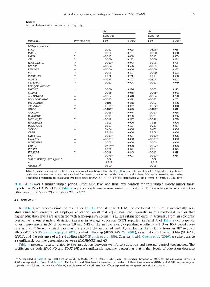
In Table 3 , we report estimation results for Eq. (1) . Consistent with H1A, the coefficient on EDUC is significantly neg-

ative using both measures of employee education. Recall that AQ is measured inversely, so this coefficient implies that

higher education levels are associated with higher-quality accruals (i.e., less estimation error in accruals). From an economic

perspective, a one standard deviation increase in average education (0.371 reported in Panel A of Table 2 ) corresponds

to an improvement in AQ of between 3.8 and 5.4% of the sample mean, depending whether the HQ or 10-K based mea-

sure is used. 19 Several control variables are predictably associated with AQ , including the distance from an SEC regional

office ( SECDIST ) ( Kedia and Rajgopal, 2011 ), analyst following ( AFOLLOW ) ( Yu, 2008 ), sales and cash flow volatility ( SALEVOL,

CFVOL ), and the existence of a Big 4 auditor ( BIG4 ) ( Francis et al., 1999 ). Consistent with Owens et al. (2016) , we also observe

a significantly positive association between IDIOSHOCKS and AQ .

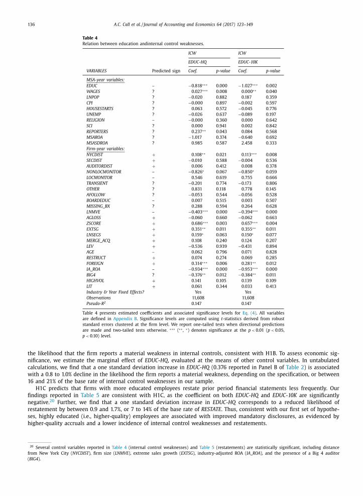
Table 4 presents results related to the association between workforce education and internal control weaknesses. The

coefficient on both EDUC-HQ and EDUC-10K are significantly negative, suggesting that higher levels of education decrease

19 As reported in Table 3 , the coefficient on EDUC-HQ ( EDUC-10K ) is -0.093 (-0.131), and the standard deviation of EDUC for the estimation sample is

0.371 (as reported in Panel A of Table 2 ). For the HQ and 10-K based measures, the product of these two values is -0.034 and -0.049, respectively, or

approximately 3.8 and 5.4 percent of the AQ sample mean of 0.9. All marginal effects reported are computed in a similar manner.

136 A.C. Call et al. / Journal of Accounting and Economics 64 (2017) 123–149

Table 4

Relation between education andinternal control weaknesses.

ICW ICW

EDUC-HQ EDUC-10K

VARIABLES Predicted sign Coef. p-value Coef. p-value

MSA-year variables:

EDUC – −0 .818 ∗∗∗ 0 .0 0 0 −1 .027 ∗∗∗ 0 .002

WAGES ? 0 .027 ∗∗∗ 0 .008 0 .0 0 0 ∗∗ 0 .040

LNPOP ? −0 .020 0 .882 0 .187 0 .359

CPI ? −0 .0 0 0 0 .897 −0 .002 0 .597

HOUSESTARTS ? 0 .063 0 .572 −0 .045 0 .776

UNEMP ? −0 .026 0 .637 −0 .089 0 .197

RELIGION – −0 .0 0 0 0 .360 0 .0 0 0 0 .642

SCI ? 0 .0 0 0 0 .941 0 .002 0 .842

REPORTERS ? 0 .237 ∗∗ 0 .043 0 .084 0 .568

MSAROA ? −1 .017 0 .374 −0 .640 0 .692

MSASDROA ? 0 .985 0 .587 2 .458 0 .333

Firm-year variables:

NYCDIST + 0 .108 ∗∗ 0 .021 0 .113 ∗∗∗ 0 .008

SECDIST + −0 .010 0 .588 −0 .004 0 .536

AUDITORDIST + 0 .006 0 .412 0 .008 0 .378

NONLOCMONITOR – −0 .826 ∗ 0 .067 −0 .850 ∗ 0 .059

LOCMONITOR – 0 .546 0 .619 0 .755 0 .666

TRANSIENT ? −0 .201 0 .774 −0 .173 0 .806

OTHER ? 0 .831 0 .118 0 .778 0 .145

AFOLLOW ? −0 .053 0 .544 −0 .056 0 .528

BOARDEDUC – 0 .007 0 .515 0 .003 0 .507

MISSING_BX ? 0 .288 0 .594 0 .264 0 .628

LNMVE – −0 .403 ∗∗∗ 0 .0 0 0 −0 .394 ∗∗∗ 0 .0 0 0

AGLOSS + −0 .060 0 .660 −0 .062 0 .663

ZSCORE + 0 .686 ∗∗∗ 0 .003 0 .657 ∗∗∗ 0 .004

EXTSG + 0 .351 ∗∗ 0 .011 0 .355 ∗∗ 0 .011

LNSEGS + 0 .159 ∗ 0 .063 0 .150 ∗ 0 .077

MERGE_ACQ + 0 .108 0 .240 0 .124 0 .207

LEV + −0 .536 0 .939 −0 .431 0 .894

AGE – 0 .062 0 .796 0 .071 0 .828

RESTRUCT + 0 .074 0 .274 0 .069 0 .285

FOREIGN + 0 .314 ∗∗∗ 0 .006 0 .281 ∗∗ 0 .012

IA_ROA – −0 .934 ∗∗∗ 0 .0 0 0 −0 .953 ∗∗∗ 0 .0 0 0

BIG4 ? −0 .376 ∗∗ 0 .012 −0 .384 ∗∗ 0 .011

HIGHVOL + 0 .141 0 .105 0 .139 0 .109

LIT + 0 .061 0 .344 0 .033 0 .413

Industry & Year Fixed Effects? Yes Yes

Observations 11,608 11,608

Pseudo-R 2 0 .147 0 .147

Table 4 presents estimated coefficients and associated significance levels for Eq. (4) . All variables

are defined in Appendix B . Significance levels are computed using t- statistics derived from robust

standard errors clustered at the firm level. We report one-tailed tests when directional predictions

are made and two-tailed tests otherwise. ∗∗∗ ( ∗∗ , ∗) denotes significance at the p < 0.01 ( p < 0.05,

p < 0.10) level.

the likelihood that the firm reports a material weakness in internal controls, consistent with H1B. To assess economic sig-

nificance, we estimate the marginal effect of EDUC-HQ , evaluated at the means of other control variables. In untabulated

calculations, we find that a one standard deviation increase in EDUC-HQ (0.376 reported in Panel B of Table 2 ) is associated

with a 0.8 to 1.0% decline in the likelihood the firm reports a material weakness, depending on the specification, or between

16 and 21% of the base rate of internal control weaknesses in our sample.

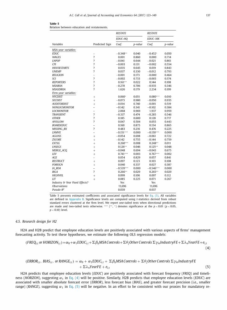
H1C predicts that firms with more educated employees restate prior period financial statements less frequently. Our

findings reported in Table 5 are consistent with H1C, as the coefficient on both EDUC-HQ and EDUC-10K are significantly

negative. 20 Further, we find that a one standard deviation increase in EDUC-HQ corresponds to a reduced likelihood of

restatement by between 0.9 and 1.7%, or 7 to 14% of the base rate of RESTATE . Thus, consistent with our first set of hypothe-

ses, highly educated (i.e., higher-quality) employees are associated with improved mandatory disclosures, as evidenced by

higher-quality accruals and a lower incidence of internal control weaknesses and restatements.

20 Several control variables reported in Table 4 (internal control weaknesses) and Table 5 (restatements) are statistically significant, including distance

from New York City ( NYCDIST ), firm size ( LNMVE ), extreme sales growth ( EXTSG ), industry-adjusted ROA ( IA_ROA ), and the presence of a Big 4 auditor

( BIG4 ).

A.C. Call et al. / Journal of Accounting and Economics 64 (2017) 123–149 137

Table 5

Relation between education and restatements.

RESTATE RESTATE

EDUC-HQ EDUC-10K

Variables Predicted Sign Coef. p-value Coef. p-value

MSA-year variables:

EDUC – −0 .348 ∗∗ 0 .040 −0 .452 ∗ 0 .050

WAGES ? 0 .001 0 .860 0 .0 0 0 0 .714

LNPOP ? −0 .041 0 .644 −0 .021 0 .861

CPI ? −0 .003 0 .131 −0 .002 0 .554

HOUSESTARTS ? 0 .035 0 .645 0 .019 0 .843

UNEMP ? 0 .037 0 .330 −0 .012 0 .793

RELIGION – −0 .001 0 .173 −0 .0 0 0 0 .464

SCI ? −0 .002 0 .733 −0 .003 0 .574

REPORTERS ? 0 .161 ∗∗ 0 .022 0 .144 0 .108

MSAROA ? −0 .270 0 .706 −0 .935 0 .346

MSASDROA ? 1 .626 0 .179 2 .234 0 .199

Firm-year variables:

NYCDIST + 0 .060 ∗ 0 .051 0 .080 ∗∗∗ 0 .010

SECDIST + −0 .073 0 .980 −0 .050 0 .935

AUDITORDIST + −0 .014 0 .740 −0 .001 0 .519

NONLOCMONITOR – −0 .142 0 .341 −0 .102 0 .384

LOCMONITOR – 2 .068 0 .969 1 .937 0 .959

TRANSIENT ? −0 .337 0 .474 −0 .285 0 .546

OTHER ? 0 .185 0 .600 0 .128 0 .717

AFOLLOW ? 0 .047 0 .504 0 .055 0 .443

BOARDEDUC – 0 .160 0 .875 0 .154 0 .865

MISSING_BX ? 0 .483 0 .216 0 .476 0 .225

LNMVE – −0 .151 ∗∗∗ 0 .0 0 0 −0 .150 ∗∗∗ 0 .0 0 0

AGLOSS + −0 .054 0 .698 −0 .061 0 .722

ZSCORE + −0 .142 0 .755 −0 .144 0 .759

EXTSG + 0 .260 ∗∗∗ 0 .008 0 .248 ∗∗ 0 .011

LNSEGS + 0 .126 ∗∗ 0 .046 0 .125 ∗∗ 0 .048

MERGE_ACQ + −0 .048 0 .694 −0 .043 0 .675

LEV + 0 .741 ∗∗∗ 0 .003 0 .767 ∗∗∗ 0 .002

AGE – 0 .054 0 .829 0 .057 0 .841

RESTRUCT + 0 .097 0 .123 0 .103 0 .108

FOREIGN + 0 .040 0 .337 0 .027 0 .387

IA_ROA – −0 .539 ∗∗∗ 0 .0 0 0 −0 .546 ∗∗∗ 0 .0 0 0

BIG4 ? 0 .266 ∗∗ 0 .029 0 .265 ∗∗ 0 .029

HIGHVOL + 0 .099 0 .106 0 .097 0 .112

LIT + 0 .085 0 .225 0 .071 0 .267

Industry & Year Fixed Effects? Yes Yes

Observations 11,696 11,696

Pseudo-R 2 0 .039 0 .037

Table 5 presents estimated coefficients and associated significance levels for Eq. (5) . All variables

are defined in Appendix B . Significance levels are computed using t- statistics derived from robust

standard errors clustered at the firm level. We report one-tailed tests when directional predictions

are made and two-tailed tests otherwise. ∗∗∗ ( ∗∗ , ∗) denotes significance at the p < 0.01 ( p < 0.05,

p < 0.10) level.

4.5. Research design for H2

H2A and H2B predict that employee education levels are positively associated with various aspects of firms’ management

forecasting activity. To test these hypotheses, we estimate the following OLS regression models:

( F RE Q i,t or HORIZO N i,t ) = α0 + α1 EDU C i,t +�βk MSA Controls+�θ j Other Controls �γm

Industr yF E+�λn Year F E+ e i,t

(4)

( ERRO R i,t , BIA S i,t , or RANG E i,t ) = α0 + α1 EDU C i,t + �βk MSA Controls + �θ j Other Controls �γm

IndustryF E

+ �λn YearF E + e i,t (5)

H2A predicts that employee education levels ( EDUC ) are positively associated with forecast frequency ( FREQ ) and timeli-

ness ( HORIZON ), suggesting α1 in Eq. (4) will be positive. Similarly, H2B predicts that employee education levels ( EDUC ) are

associated with smaller absolute forecast error ( ERROR ), less forecast bias ( BIAS ), and greater forecast precision (i.e., smaller

range) ( RANGE ), suggesting α in Eq. (5) will be negative. In an effort to be consistent with our proxies for mandatory re-

1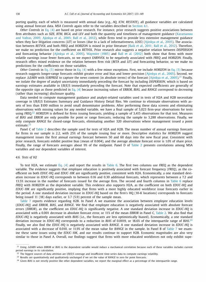

138 A.C. Call et al. / Journal of Accounting and Economics 64 (2017) 123–149

porting quality, each of which is measured with annual data (e.g., AQ, ICW, RESTATE ), all guidance variables are calculated

using annual forecast data. MSA Controls again refer to the variables described in Section 4.1 .

Other Controls in Eq. (4) are based on prior research. For instance, prior research suggests positive associations between

firm attributes such as SIZE, BTM, BIG4, and LEV and both the quantity and timeliness of management guidance ( Karamanou

and Vafeas, 2005; Ajinkya et al., 2005; Ball et al., 2012 ), while firms tend to provide less extensive management guidance

when they face litigation concerns ( LIT ) or losses (due to a lack of informativeness, LOSS ) ( Ajinkya et al., 2005 ). The associa-

tion between RETVOL and both FREQ and HORIZON is mixed in prior literature ( Baik et al., 2011; Ball et al., 2012 ). Therefore,

we make no prediction for the coefficient on RETVOL . Prior research also suggests a negative relation between DISPERSION

and forecasting behavior ( Ajinkya et al., 2005 ). Waymire (1985) and Ball et al. (2012) both show that firms with more

volatile earnings issue fewer forecasts, so we expect EARNVOL to be negatively associated with FREQ and HORIZON. Finally,

research offers mixed evidence on the relation between firm risk ( BETA and LIT ) and forecasting behavior, so we make no

predictions for the coefficients on those variables.

Other Controls in Eq. (5) mirror those in Eq. (4) with a few minor exceptions. First, we include HORIZON in Eq. (5) because

research suggests longer-range forecasts exhibit greater error and bias and lower precision ( Ajinkya et al., 2005 ). Second, we

replace �EARN with SURPRISE to capture the news content (in absolute terms) of the forecast ( Ajinkya et al., 2005 ). 21 Finally,

we isolate the degree of analyst uncertainty immediately preceding the forecast by including DISPERSION , which is based on

earnings estimates available in I/B/E/S immediately preceding the forecast. Note that expected coefficients are generally of

the opposite sign as those predicted in Eq. (4) because increasing values of ERROR, BIAS, and RANGE correspond to decreasing

(rather than increasing ) disclosure quality.

Data needed to compute management guidance and analyst-related variables used in tests of H2A and H2B necessitate

coverage in I/B/E/S Estimates Summary and Guidance History Detail files. We continue to eliminate observations with as-

sets of less than $100 million to avoid small denominator problems. After performing these data screens and eliminating

observations with missing values for any needed variable, we have a final sample of 5,023 firm-year observations for tests

using FREQ . 22 HORIZON is defined for firms issuing forecasts, yielding a sample of 3,415 observations for that test. Measures

of BIAS and ERROR are only possible for point or range forecasts, reducing the sample to 3,288 observations. Finally, we

only compute RANGE for closed-range forecasts, eliminating another 320 observations where management issued a point

estimate. 23

Panel C of Table 2 describes the sample used for tests of H2A and H2B. The mean number of annual earnings forecasts

for firms in our sample is 2.2, with 25% of the sample issuing four or more. Descriptive statistics for HORIZON suggest

management issues the first annual earnings forecast between 50 and 60 days into the new fiscal year. Consistent with

prior research, forecasts exhibit positive bias (mean of 0.004), and the average absolute forecast error is 1.0% of share price.

Finally, the range of forecasts averages about 9% of the midpoint. Panel D of Table 2 presents correlations among MSA

variables and our dependent variables of interest.

4.6. Tests of H2

To test H2A, we estimate Eq. (4) and report the results in Table 6 . The first two columns use FREQ as the dependent

variable. The evidence suggests that employee education is positively associated with forecast frequency ( FREQ ), as the co-

efficient on both EDUC-HQ and EDUC-10K are significantly positive, consistent with H2A. Economically, a one standard devi-

ation increase in EDUC-HQ corresponds to between 0.16 and 0.30 additional forecasts, which represents between a 7.2 and

13.5% increase in the number of forecasts issued for the average firm. The second and fourth columns in Table 6 replace

FREQ with HORIZON as the dependent variable. This evidence also supports H2A, as the coefficient on both EDUC-HQ and

EDUC-10K are significantly positive, implying that firms with a more highly educated workforce issue forecasts earlier in

the period. A one standard deviation increase in EDUC-HQ based on the firm’s HQ (10-K locations) corresponds to forecasts

being issued 11 (18) days earlier, or 3.7 (5.9) percent of the sample mean.

Table 7 reports evidence regarding H2B. In Panel A we examine the association between employee education levels

( EDUC-HQ ) and ERROR, BIAS , and RANGE . We find that employee education is negatively associated with absolute forecast

errors ( ERROR ), as the coefficient on EDUC-HQ is significantly negative. A one standard deviation increase in EDUC-HQ is

associated with a 0.001 decrease in absolute forecast error, or 11% of the mean ERROR in Panel C, Table 2 . We also find that

EDUC-HQ is negatively associated with BIAS (i.e., the forecasts are less optimistically biased). Economically, a one standard

deviation increase in EDUC-HQ corresponds to a reduction in BIAS of 0.0019, or 18.6% of the interquartile range of BIAS . 24

Finally, we also find the EDUC-HQ is negatively associated with RANGE. A one standard deviation increase in EDUC-HQ is

associated with a decrease of 0.010, or 11.9% of the mean value for RANGE in the sample. In Panel B of Table 7 we exam-

ine these same issues using the EDUC-10K , and our results continue to support H2B. Economic magnitudes are also very

similar to those in Panel A. Overall, our findings suggest that firms with more educated workforces not only exhibit supe-

21 Using �EARN when ERROR or BIAS is the dependent variable would induce a mechanical correlation because each of these variables includes current

period earnings in its calculation. 22 The biggest sources of data attrition are I/B/E/S coverage and insufficient time-series data to compute earnings volatility. 23 Results are quantitatively and qualitatively unchanged if we set the value of RANGE to zero for point forecasts. 24 Given BIAS is not strictly positive like other dependent variables, we report the marginal effect as a percentage of the interquartile range.

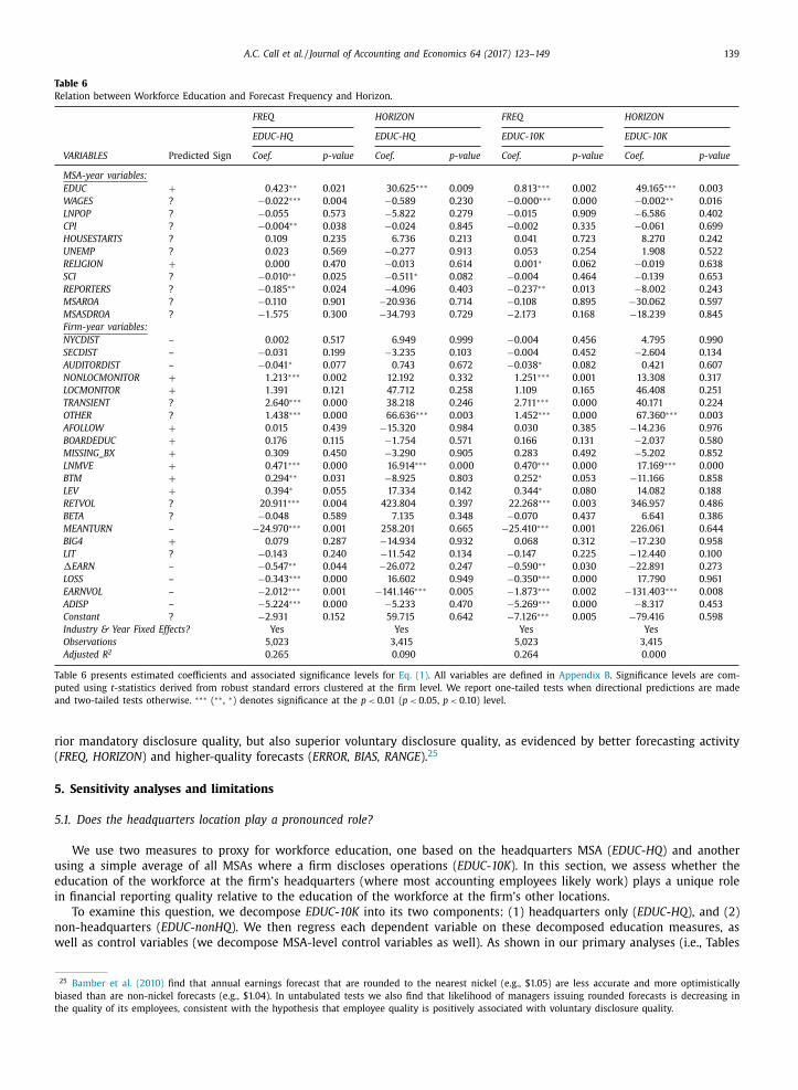
A.C. Call et al. / Journal of Accounting and Economics 64 (2017) 123–149 139

Table 6

Relation between Workforce Education and Forecast Frequency and Horizon.

FREQ HORIZON FREQ HORIZON

EDUC-HQ EDUC-HQ EDUC-10K EDUC-10K

VARIABLES Predicted Sign Coef. p-value Coef. p-value Coef. p-value Coef. p-value

MSA-year variables:

EDUC + 0 .423 ∗∗ 0 .021 30 .625 ∗∗∗ 0 .009 0 .813 ∗∗∗ 0 .002 49 .165 ∗∗∗ 0 .003

WAGES ? −0 .022 ∗∗∗ 0 .004 −0 .589 0 .230 −0 .0 0 0 ∗∗∗ 0 .0 0 0 −0 .002 ∗∗ 0 .016

LNPOP ? −0 .055 0 .573 −5 .822 0 .279 −0 .015 0 .909 −6 .586 0 .402

CPI ? −0 .004 ∗∗ 0 .038 −0 .024 0 .845 −0 .002 0 .335 −0 .061 0 .699

HOUSESTARTS ? 0 .109 0 .235 6 .736 0 .213 0 .041 0 .723 8 .270 0 .242

UNEMP ? 0 .023 0 .569 −0 .277 0 .913 0 .053 0 .254 1 .908 0 .522

RELIGION + 0 .0 0 0 0 .470 −0 .013 0 .614 0 .001 ∗ 0 .062 −0 .019 0 .638

SCI ? −0 .010 ∗∗ 0 .025 −0 .511 ∗ 0 .082 −0 .004 0 .464 −0 .139 0 .653

REPORTERS ? −0 .185 ∗∗ 0 .024 −4 .096 0 .403 −0 .237 ∗∗ 0 .013 −8 .002 0 .243

MSAROA ? −0 .110 0 .901 −20 .936 0 .714 −0 .108 0 .895 −30 .062 0 .597

MSASDROA ? −1 .575 0 .300 −34 .793 0 .729 −2 .173 0 .168 −18 .239 0 .845

Firm-year variables:

NYCDIST – 0 .002 0 .517 6 .949 0 .999 −0 .004 0 .456 4 .795 0 .990

SECDIST – −0 .031 0 .199 −3 .235 0 .103 −0 .004 0 .452 −2 .604 0 .134

AUDITORDIST – −0 .041 ∗ 0 .077 0 .743 0 .672 −0 .038 ∗ 0 .082 0 .421 0 .607

NONLOCMONITOR + 1 .213 ∗∗∗ 0 .002 12 .192 0 .332 1 .251 ∗∗∗ 0 .001 13 .308 0 .317

LOCMONITOR + 1 .391 0 .121 47 .712 0 .258 1 .109 0 .165 46 .408 0 .251

TRANSIENT ? 2 .640 ∗∗∗ 0 .0 0 0 38 .218 0 .246 2 .711 ∗∗∗ 0 .0 0 0 40 .171 0 .224

OTHER ? 1 .438 ∗∗∗ 0 .0 0 0 66 .636 ∗∗∗ 0 .003 1 .452 ∗∗∗ 0 .0 0 0 67 .360 ∗∗∗ 0 .003

AFOLLOW + 0 .015 0 .439 −15 .320 0 .984 0 .030 0 .385 −14 .236 0 .976

BOARDEDUC + 0 .176 0 .115 −1 .754 0 .571 0 .166 0 .131 −2 .037 0 .580

MISSING_BX + 0 .309 0 .450 −3 .290 0 .905 0 .283 0 .492 −5 .202 0 .852

LNMVE + 0 .471 ∗∗∗ 0 .0 0 0 16 .914 ∗∗∗ 0 .0 0 0 0 .470 ∗∗∗ 0 .0 0 0 17 .169 ∗∗∗ 0 .0 0 0

BTM + 0 .294 ∗∗ 0 .031 −8 .925 0 .803 0 .252 ∗ 0 .053 −11 .166 0 .858

LEV + 0 .394 ∗ 0 .055 17 .334 0 .142 0 .344 ∗ 0 .080 14 .082 0 .188

RETVOL ? 20 .911 ∗∗∗ 0 .004 423 .804 0 .397 22 .268 ∗∗∗ 0 .003 346 .957 0 .486

BETA ? −0 .048 0 .589 7 .135 0 .348 −0 .070 0 .437 6 .641 0 .386

MEANTURN – −24 .970 ∗∗∗ 0 .001 258 .201 0 .665 −25 .410 ∗∗∗ 0 .001 226 .061 0 .644

BIG4 + 0 .079 0 .287 −14 .934 0 .932 0 .068 0 .312 −17 .230 0 .958

LIT ? −0 .143 0 .240 −11 .542 0 .134 −0 .147 0 .225 −12 .440 0 .100

�EARN – −0 .547 ∗∗ 0 .044 −26 .072 0 .247 −0 .590 ∗∗ 0 .030 −22 .891 0 .273

LOSS – −0 .343 ∗∗∗ 0 .0 0 0 16 .602 0 .949 −0 .350 ∗∗∗ 0 .0 0 0 17 .790 0 .961

EARNVOL – −2 .012 ∗∗∗ 0 .001 −141 .146 ∗∗∗ 0 .005 −1 .873 ∗∗∗ 0 .002 −131 .403 ∗∗∗ 0 .008

ADISP – −5 .224 ∗∗∗ 0 .0 0 0 −5 .233 0 .470 −5 .269 ∗∗∗ 0 .0 0 0 −8 .317 0 .453

Constant ? −2 .931 0 .152 59 .715 0 .642 −7 .126 ∗∗∗ 0 .005 −79 .416 0 .598

Industry & Year Fixed Effects? Yes Yes Yes Yes

Observations 5,023 3,415 5,023 3,415

Adjusted R 2 0 .265 0 .090 0 .264 0 .0 0 0

Table 6 presents estimated coefficients and associated significance levels for Eq. (1) . All variables are defined in Appendix B . Significance levels are com-

puted using t- statistics derived from robust standard errors clustered at the firm level. We report one-tailed tests when directional predictions are made

and two-tailed tests otherwise. ∗∗∗ ( ∗∗ , ∗) denotes significance at the p < 0.01 ( p < 0.05, p < 0.10) level.

rior mandatory disclosure quality, but also superior voluntary disclosure quality, as evidenced by better forecasting activity

( FREQ, HORIZON ) and higher-quality forecasts ( ERROR, BIAS, RANGE ). 25

5. Sensitivity analyses and limitations

5.1. Does the headquarters location play a pronounced role?

We use two measures to proxy for workforce education, one based on the headquarters MSA ( EDUC-HQ ) and another

using a simple average of all MSAs where a firm discloses operations ( EDUC-10K ). In this section, we assess whether the

education of the workforce at the firm’s headquarters (where most accounting employees likely work) plays a unique role

in financial reporting quality relative to the education of the workforce at the firm’s other locations.

To examine this question, we decompose EDUC-10K into its two components: (1) headquarters only ( EDUC-HQ ), and (2)

non-headquarters ( EDUC-nonHQ ). We then regress each dependent variable on these decomposed education measures, as

well as control variables (we decompose MSA-level control variables as well). As shown in our primary analyses (i.e., Tables

25 Bamber et al. (2010) find that annual earnings forecast that are rounded to the nearest nickel (e.g., $1.05) are less accurate and more optimistically

biased than are non-nickel forecasts (e.g., $1.04). In untabulated tests we also find that likelihood of managers issuing rounded forecasts is decreasing in

the quality of its employees, consistent with the hypothesis that employee quality is positively associated with voluntary disclosure quality.

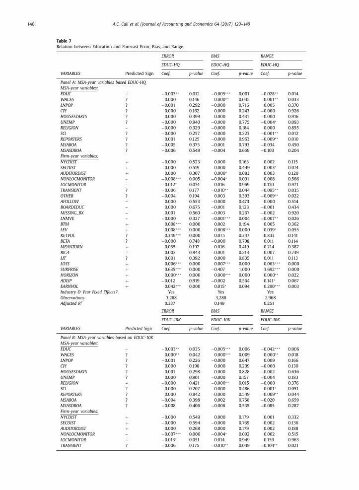
140 A.C. Call et al. / Journal of Accounting and Economics 64 (2017) 123–149

Table 7

Relation between Education and Forecast Error, Bias, and Range.

ERROR BIAS RANGE

EDUC-HQ EDUC-HQ EDUC-HQ

VARIABLES Predicted Sign Coef. p-value Coef. p-value Coef. p-value

Panel A: MSA-year variables based EDUC-HQ

MSA-year variables:

EDUC – −0 .003 ∗∗ 0 .012 −0 .005 ∗∗∗ 0 .001 −0 .028 ∗∗ 0 .014

WAGES ? 0 .0 0 0 0 .146 0 .0 0 0 ∗∗ 0 .045 0 .001 ∗∗ 0 .033

LNPOP ? −0 .001 0 .292 −0 .0 0 0 0 .716 0 .005 0 .370

CPI ? 0 .0 0 0 0 .162 0 .0 0 0 0 .243 −0 .0 0 0 0 .926

HOUSESTARTS ? 0 .0 0 0 0 .399 0 .0 0 0 0 .431 −0 .0 0 0 0 .916

UNEMP ? −0 .0 0 0 0 .940 −0 .0 0 0 0 .775 −0 .004 ∗ 0 .093

RELIGION – −0 .0 0 0 0 .329 −0 .0 0 0 0 .184 0 .0 0 0 0 .855

SCI ? −0 .0 0 0 0 .257 -0 .0 0 0 0 .223 −0 .001 ∗∗ 0 .012

REPORTERS ? 0 .001 0 .125 −0 .0 0 0 0 .963 −0 .009 ∗∗ 0 .010

MSAROA ? −0 .005 0 .375 −0 .001 0 .793 −0 .034 0 .450

MSASDROA ? −0 .006 0 .549 −0 .004 0 .659 −0 .103 0 .204

Firm-year variables:

NYCDIST + −0 .0 0 0 0 .523 0 .0 0 0 0 .163 0 .002 0 .115

SECDIST + −0 .0 0 0 0 .519 0 .0 0 0 0 .449 0 .003 ∗ 0 .074

AUDITORDIST + 0 .0 0 0 0 .307 0 .0 0 0 ∗ 0 .083 0 .003 0 .120

NONLOCMONITOR – −0 .008 ∗∗∗ 0 .005 −0 .004 ∗ 0 .091 0 .008 0 .566

LOCMONITOR – −0 .012 ∗ 0 .074 0 .016 0 .969 0 .170 0 .971

TRANSIENT ? −0 .006 0 .177 −0 .010 ∗∗ 0 .044 −0 .095 ∗∗ 0 .035

OTHER ? −0 .004 0 .194 0 .003 0 .393 −0 .069 ∗∗ 0 .022

AFOLLOW – 0 .0 0 0 0 .553 −0 .0 0 0 0 .473 0 .0 0 0 0 .514

BOARDEDUC – 0 .0 0 0 0 .675 −0 .001 0 .123 −0 .001 0 .434

MISSING_BX – 0 .001 0 .560 −0 .003 0 .267 −0 .002 0 .920

LNMVE – −0 .0 0 0 0 .327 −0 .001 ∗∗∗ 0 .004 −0 .007 ∗∗ 0 .026

BTM + 0 .008 ∗∗∗ 0 .0 0 0 0 .002 0 .194 0 .005 0 .362

LEV + 0 .008 ∗∗∗ 0 .0 0 0 0 .008 ∗∗∗ 0 .0 0 0 0 .039 ∗ 0 .055

RETVOL ? 0 .349 ∗∗∗ 0 .0 0 0 0 .075 0 .347 0 .833 0 .141

BETA ? −0 .0 0 0 0 .748 −0 .0 0 0 0 .708 0 .011 0 .114

MEANTURN + 0 .055 0 .197 0 .016 0 .419 0 .214 0 .387

BIG4 – 0 .002 0 .943 −0 .001 0 .213 0 .007 0 .739

LIT ? 0 .001 0 .392 0 .0 0 0 0 .835 0 .011 0 .113

LOSS + 0 .006 ∗∗∗ 0 .0 0 0 0 .007 ∗∗∗ 0 .0 0 0 0 .063 ∗∗∗ 0 .0 0 0

SURPRISE + 0 .635 ∗∗∗ 0 .0 0 0 −0 .407 1 .0 0 0 3 .692 ∗∗∗ 0 .0 0 0

HORIZON + 0 .0 0 0 ∗∗∗ 0 .0 0 0 0 .0 0 0 ∗∗∗ 0 .0 0 0 0 .0 0 0 ∗∗ 0 .022

ADISP + −0 .012 0 .919 −0 .002 0 .564 0 .141 ∗ 0 .067

EARNVOL + 0 .042 ∗∗∗ 0 .0 0 0 0 .015 ∗ 0 .094 0 .290 ∗∗∗ 0 .003

Industry & Year Fixed Effects? Yes Yes Yes

Observations 3,288 3,288 2,968

Adjusted R 2 0 .337 0 .149 0 .251

ERR OR BIAS RANGE

EDUC-10K EDUC-10K EDUC-10K

VARIABLES Predicted Sign Coef. p-value Coef. p-value Coef. p-value

Panel B: MSA-year variables based on EDUC-10K

MSA-year variables:

EDUC – −0 .003 ∗∗ 0 .035 −0 .005 ∗∗∗ 0 .006 −0 .042 ∗∗∗ 0 .006

WAGES ? 0 .0 0 0 ∗∗ 0 .042 0 .0 0 0 ∗∗∗ 0 .009 0 .0 0 0 ∗∗ 0 .018

LNPOP ? −0 .001 0 .226 −0 .0 0 0 0 .647 0 .009 0 .166

CPI ? 0 .0 0 0 0 .198 0 .0 0 0 0 .209 −0 .0 0 0 0 .130

HOUSESTARTS ? 0 .001 0 .298 0 .0 0 0 0 .828 −0 .002 0 .636

UNEMP ? 0 .0 0 0 0 .901 −0 .0 0 0 0 .157 −0 .004 0 .183

RELIGION – −0 .0 0 0 0 .421 −0 .0 0 0 ∗∗ 0 .015 −0 .0 0 0 0 .376

SCI ? −0 .0 0 0 0 .207 −0 .0 0 0 0 .486 −0 .001 ∗ 0 .051

REPORTERS ? 0 .0 0 0 0 .842 −0 .0 0 0 0 .549 −0 .009 ∗∗ 0 .044

MSAROA ? −0 .004 0 .398 0 .002 0 .758 −0 .020 0 .659

MSASDROA ? −0 .008 0 .406 −0 .006 0 .535 −0 .085 0 .287

Firm-year variables:

NYCDIST + −0 .0 0 0 0 .549 0 .0 0 0 0 .179 0 .001 0 .332

SECDIST + −0 .0 0 0 0 .594 −0 .0 0 0 0 .769 0 .002 0 .136

AUDITORDIST + 0 .0 0 0 0 .268 0 .0 0 0 0 .179 0 .002 0 .188

NONLOCMONITOR – −0 .007 ∗∗∗ 0 .006 −0 .004 ∗ 0 .092 0 .002 0 .515

LOCMONITOR – −0 .013 ∗ 0 .051 0 .014 0 .949 0 .159 0 .963

TRANSIENT ? −0 .006 0 .175 −0 .010 ∗∗ 0 .049 −0 .104 ∗∗ 0 .021

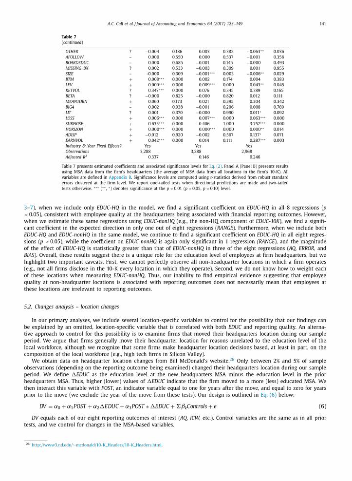
A.C. Call et al. / Journal of Accounting and Economics 64 (2017) 123–149 141

Table 7

( continued )

OTHER ? −0 .004 0 .186 0 .003 0 .382 −0 .063 ∗∗ 0 .036

AFOLLOW – 0 .0 0 0 0 .550 0 .0 0 0 0 .537 −0 .001 0 .358

BOARDEDUC – 0 .0 0 0 0 .685 −0 .001 0 .145 −0 .0 0 0 0 .493

MISSING_BX ? 0 .002 0 .533 −0 .003 0 .309 0 .001 0 .955

SIZE – -0 .0 0 0 0 .309 −0 .001 ∗∗∗ 0 .003 −0 .006 ∗∗ 0 .029

BTM + 0 .008 ∗∗∗ 0 .0 0 0 0 .002 0 .174 0 .004 0 .383

LEV + 0 .009 ∗∗∗ 0 .0 0 0 0 .009 ∗∗∗ 0 .0 0 0 0 .043 ∗∗ 0 .045

RETVOL ? 0 .347 ∗∗∗ 0 .0 0 0 0 .076 0 .345 0 .789 0 .165

BETA ? −0 .0 0 0 0 .825 −0 .0 0 0 0 .820 0 .012 0 .111

MEANTURN + 0 .060 0 .173 0 .021 0 .395 0 .304 0 .342

BIG4 – 0 .002 0 .938 −0 .001 0 .206 0 .008 0 .769

LIT ? 0 .001 0 .370 −0 .0 0 0 0 .990 0 .011 ∗ 0 .092

LOSS + 0 .006 ∗∗∗ 0 .0 0 0 0 .007 ∗∗∗ 0 .0 0 0 0 .063 ∗∗∗ 0 .0 0 0

SURPRISE + 0 .635 ∗∗∗ 0 .0 0 0 −0 .406 1 .0 0 0 3 .757 ∗∗∗ 0 .0 0 0

HORIZON + 0 .0 0 0 ∗∗∗ 0 .0 0 0 0 .0 0 0 ∗∗∗ 0 .0 0 0 0 .0 0 0 ∗∗ 0 .014

ADISP + −0 .012 0 .920 −0 .002 0 .567 0 .137 ∗ 0 .071

EARNVOL + 0 .042 ∗∗∗ 0 .0 0 0 0 .014 0 .111 0 .287 ∗∗∗ 0 .003

Industry & Year Fixed Effects? Yes Yes Yes

Observations 3,288 3,288 2,968

Adjusted R 2 0 .337 0 .146 0 .246

Table 7 presents estimated coefficients and associated significance levels for Eq. (2) . Panel A (Panel B) presents results

using MSA data from the firm’s headquarters (the average of MSA data from all locations in the firm’s 10-K). All

variables are defined in Appendix B . Significance levels are computed using t- statistics derived from robust standard

errors clustered at the firm level. We report one-tailed tests when directional predictions are made and two-tailed

tests otherwise. ∗∗∗ ( ∗∗ , ∗) denotes significance at the p < 0.01 ( p < 0.05, p < 0.10) level.

3 –7 ), when we include only EDUC-HQ in the model, we find a significant coefficient on EDUC-HQ in all 8 regressions ( p

< 0.05), consistent with employee quality at the headquarters being associated with financial reporting outcomes. However,

when we estimate these same regressions using EDUC-nonHQ (e.g., the non-HQ component of EDUC-10K ), we find a signifi-

cant coefficient in the expected direction in only one out of eight regressions ( RANGE ). Furthermore, when we include both

EDUC-HQ and EDUC-nonHQ in the same model, we continue to find a significant coefficient on EDUC-HQ in all eight regres-

sions ( p < 0.05), while the coefficient on EDUC-nonHQ is again only significant in 1 regression (RANGE ) , and the magnitude

of the effect of EDUC-HQ is statistically greater than that of EDUC-nonHQ in three of the eight regressions ( AQ, ERROR, and

BIAS ). Overall, these results suggest there is a unique role for the education level of employees at firm headquarters, but we

highlight two important caveats. First, we cannot perfectly observe all non-headquarter locations in which a firm operates

(e.g., not all firms disclose in the 10-K every location in which they operate). Second, we do not know how to weight each

of these locations when measuring EDUC-nonHQ . Thus, our inability to find empirical evidence suggesting that employee

quality at non-headquarter locations is associated with reporting outcomes does not necessarily mean that employees at

these locations are irrelevant to reporting outcomes.

5.2. Changes analysis – location changes

In our primary analyses, we include several location-specific variables to control for the possibility that our findings can

be explained by an omitted, location-specific variable that is correlated with both EDUC and reporting quality. An alterna-

tive approach to control for this possibility is to examine firms that moved their headquarters location during our sample

period. We argue that firms generally move their headquarter location for reasons unrelated to the education level of the

local workforce, although we recognize that some firms make headquarter location decisions based, at least in part, on the

composition of the local workforce (e.g., high tech firms in Silicon Valley).

We obtain data on headquarter location changes from Bill McDonald’s website. 26 Only between 2% and 5% of sample

observations (depending on the reporting outcome being examined) changed their headquarters location during our sample

period. We define �EDUC as the education level at the new headquarters MSA minus the education level in the prior

headquarters MSA. Thus, higher (lower) values of �EDUC indicate that the firm moved to a more (less) educated MSA. We

then interact this variable with POST , an indicator variable equal to one for years after the move, and equal to zero for years

prior to the move (we exclude the year of the move from these tests). Our design is outlined in Eq. (6) below:

DV = α0 + α1 P OST + α2 �EDUC + α3 P OST ∗ �EDUC + �βk Controls + e (6)

DV equals each of our eight reporting outcomes of interest ( AQ, ICW, etc . ). Control variables are the same as in all prior

tests, and we control for changes in the MSA-based variables.

26 http://www3.nd.edu/ ∼mcdonald/10-K _ Headers/10-K _ Headers.html .

142 A.C. Call et al. / Journal of Accounting and Economics 64 (2017) 123–149

We assume that when a firm moves its headquarters, the firm employs more individuals from the new headquarters

location than was true prior to the move. 27 If α3 loads in the same direction as was originally predicted (e.g., negative for

accrual quality, positive for forecast frequency), it suggests that changes in employee education levels at the firm’s head-

quarters are associated with predictable changes in reporting outcomes in the period following the move.

We find the coefficient on this interaction loads in the predicted direction in six out of eight regressions. More impor-

tantly, despite very small sample sizes ( N as low as 75) and resulting lack of statistical power, four of the individual results

are statistically significant on their own (for H1, accrual quality ( AQ ) and restatements ( RESTATE ); for H2, management fore-

cast error ( ERROR ), and management forecast range ( RANGE )). In untabulated tests, we also find similar results when we

examine non-headquarter employee changes (in place of headquarter changes), providing some evidence that non-HQ em-

ployees can affect reporting outcomes as well. 28

In summary, these location change tests provide some additional evidence that changes in the average education level

of a firm’s employees is positively associated with changes in both external and internal reporting quality. However, we

interpret these results with caution given the very small number of observations upon which these tests are based.

5.3. High-quality employees and the likelihood of whistleblowing activity

While our hypotheses predict that EDUC is associated with improved reporting outcomes, prior literature shows that

employees can impose ex-post discipline on the firm’s financial reporting (i.e., after fraudulent behavior has occurred) by

blowing the whistle to external parties ( Dyck et al., 2010; Bowen et al., 2010 ). Thus, we examine whether, conditional on a

misreporting event, the education level of the firm’s workforce is positively associated with the likelihood that an employee

reports the violation to a regulator. We utilize the OSHA-based sample of whistleblowing violations described in Bowen

et al. (2010), Wilde (2017) , and Call et al. (2017) . This data contains instances in which an employee whistleblower files a

complaint with OSHA for workplace discrimination for having voiced concerns about financial reporting issues.

We use Audit Analytics’ Non-reliance data as our sample of misreporting firms, and set WHISTLE equal to one if a whistle-

blowing allegation occurs between the beginning of the restatement period and the date of restatement announcement, and

zero otherwise. 29 We then estimate the following model:

P r ( W HIST LE = 1 ) = (α0 + α1 EDU C i,t + �βk MSA Controls + �θ j Other Controls �γm

Industr yF E + �λn Year F E )

(7)

Other Controls are largely derived from Bowen et al. (2010) and include measures of operating results ( SALESGROWTH,

DOWNSIZE, PERFORMANCE) , opportunity and incentive for whistleblowing ( QUITAM, ICW ), size ( LNSALE) , reputation ( REPUTA-

TION ), age ( AGE ), investment ( RD_SALES ), and restatement severity ( DURATION ). We expect each of these measures to relate

positively to WHISTLE .

We report these results in Table 8 . We observe a significantly positive association between EDUC-HQ and WHISTLE , con-

sistent with more highly educated employees being more likely to uncover financial impropriety. However, we fail to observe

a positive and significant relation between EDUC-10K and WHISTLE. This evidence provides some support for the notion that,

even after reporting violations occur, more highly educated employees, particularly those working at a firm’s headquarters,

provide superior disciplining of senior management.

5.4. Firm fixed effects

In our primary tests, we include a series of location-specific control variables, industry and year fixed effects, and in

analyses above we also examine cases where the firm changes its headquarters location. To further consider the possibility

of a correlated omitted variable, we examine the sensitivity of our results to firm fixed effects. Firm fixed effects control for

any time-invariant correlated omitted variable.

27 In untabulated results, we find that firms moving headquarters experience a larger increase in employees from year t -1 to year t + 1 (24 percent increase

in employees) than do all other firm-year observations in our sample (13 percent, t = 4.00), consistent with the notion that these firms are likely to hire

additional employees from the new headquarters location. 28 Specifically, we identify all firms in our sample (a) that mention a different set of locations in its 10-K relative to the locations mentioned in its

prior 10-K, and (b) where the absolute change in the number of firm-wide employees exceeds 10%. We argue that these firms experienced a meaningful

change in the composition and location of its non-headquarter employees from one year to the next. When we estimate a model similar to Eq. (6) , but

where �EDUC captures the change in non-headquarter employee quality and without the interaction terms (because firms can change locations multiple

times), we find some support for H1 (fewer ICW, p -value = 0.098) and H2 (higher FREQ, p -value = 0.051; smaller ERROR, p -value = 0.006; narrower RANGE, p -

value = 0.012). However, we fail to find results for AQ, RESTATE, HORIZON , and BIAS . As with our change in headquarter tests, we interpret these results with

caution given the relative infrequency of large changes in the number of employees. However, this evidence provides some support for non-headquarter

employees being associated with financial reporting outcomes. 29 Because our whistleblowing data ends in March of 2010, we delete restatements announced after this date. Further, our first year of education data is

2005, so our sample is limited to restatements that started in 2006 or later and that were announced prior to March 2010. We measure EDUC (and other

variables) as of the beginning of the restatement period, and estimate Eq. (3) using just one observation for each firm. If a firm has a restatement during

this sample period, we retain that firm-year observation in this analysis. If a firm has multiple restatements during this period, and none correspond to a

whistleblowing allegation, we retain the first restatement in our sample period.

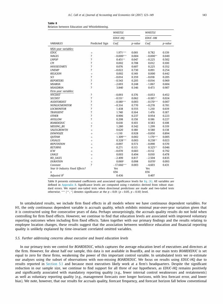
A.C. Call et al. / Journal of Accounting and Economics 64 (2017) 123–149 143

Table 8

Relation between Education and Whistleblowing.

WHISTLE WHISTLE

EDUC-HQ EDUC-10K

VARIABLES Predicted Sign Coef. p-value Coef. p-value

MSA-year variables:

EDUC + 1 .971 ∗∗∗ 0 .001 0 .782 0 .139

WAGES ? −0 .0 0 0 ∗∗∗ 0 .004 −0 .0 0 0 ∗∗ 0 .049

LNPOP ? 0 .451 ∗∗ 0 .047 −0 .225 0 .502

CPI ? 0 .002 0 .708 0 .012 0 .100

HOUSESTARTS ? 0 .076 0 .607 0 .225 0 .352

UNEMP ? −0 .022 0 .730 0 .091 0 .254

RELIGION + 0 .002 0 .149 0 .0 0 0 0 .442

SCI ? −0 .014 0 .359 −0 .018 0 .205

REPORTERS ? −0 .543 0 .205 −0 .014 0 .969

MSAROA ? −2 .693 0 .248 −1 .067 0 .604

MSASDROA ? 3 .840 0 .346 0 .473 0 .907

Firm-year variables:

NYCDIST ? −0 .093 0 .376 −0 .053 0 .452

SECDIST ? −0 .151 ∗ 0 .062 −0 .185 ∗∗ 0 .024

AUDITORDIST ? −0 .180 ∗∗∗ 0 .003 −0 .170 ∗∗∗ 0 .007

NONLOCMONITOR ? −0 .314 0 .770 −0 .278 0 .781

LOCMONITOR ? 1 .438 0 .555 1 .210 0 .619

TRANSIENT ? 1 .740 0 .164 1 .476 0 .187

OTHER ? 0 .906 0 .237 0 .954 0 .223

AFOLLOW ? 0 .208 0 .158 0 .186 0 .227

BOARDEDUC + 0 .618 0 .103 0 .583 0 .108

MISSING_BX ? 1 .280 0 .342 1 .299 0 .319

SALESGROWTH + 0 .620 0 .180 0 .580 0 .138

DOWNSIZE + −1 .110 0 .928 −0 .850 0 .894

QUITAM + 1 .309 ∗∗∗ 0 .002 1 .170 ∗∗∗ 0 .005

LNSALES + 0 .328 ∗∗∗ 0 .003 0 .238 ∗∗ 0 .023

REPUTATION + −0 .097 0 .573 −0 .090 0 .570

RETURNS + 0 .271 0 .113 0 .325 ∗∗ 0 .046

ICW + −0 .070 0 .683 −0 .112 0 .792

LNAGE + 0 .003 0 .494 0 .010 0 .478

RD_SALES + −2 .499 0 .817 −2 .504 0 .835

DURATION + 0 .069 ∗ 0 .098 0 .070 ∗ 0 .093

Constant ? −17 .666 ∗∗∗ 0 .003 −4 .603 0 .431

Year & Industry Fixed Effects? Yes Yes

n 656 656

Adjusted R 2 0 .436 0 .407

Table 8 presents estimated coefficients and associated significance levels for Eq. (6) . All variables are

defined in Appendix B . Significance levels are computed using t- statistics derived from robust stan-

dard errors. We report one-tailed tests when directional predictions are made and two-tailed tests

otherwise. ∗∗∗ ( ∗∗ , ∗) denotes significance at the p < 0.01 ( p < 0.05, p < 0.10) level.

In untabulated results, we include firm fixed effects in all models where we have continuous dependent variables. For

H1, the only continuous dependent variable is accruals quality, which exhibits minimal year-over-year variation given that

it is constructed using five consecuti ve years of data. Perhaps unsurprisingly, the accruals quality results do not hold when

controlling for firm fixed effects. However, we continue to find that education levels are associated with improved voluntary

reporting outcomes when including firm fixed effects. Taken together with our primary findings and the results relating to

employee location changes, these results suggest that the association between workforce education and financial reporting

quality is unlikely explained by time-invariant correlated omitted variables.

5.5. Further addressing concerns about executive and board education levels

In our primary tests we control for BOARDEDUC , which captures the average education level of executives and directors at

the firm. However, for about half our sample, this data is not available in BoardEx, and in our main tests BOARDEDUC is set

equal to zero for these firms, weakening the power of this important control variable. In untabulated tests we re-estimate

our analyses using the subset of observations with non-missing BOARDEDUC . We focus on results using EDUC-HQ due to

results reported in Section 5.1 and because most executives likely work at a firm’s headquarters. Despite the significant

reduction in our sample size, we continue to find support for all three of our hypotheses, as EDUC-HQ remains positively

and significantly associated with mandatory reporting quality (e.g., fewer internal control weaknesses and restatements)

as well as voluntary reporting quality (e.g., management forecasts over longer horizons, with less forecast error, and lower

bias). We note, however, that our results for accruals quality, forecast frequency, and forecast horizon fall below conventional

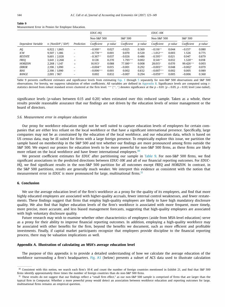
144 A.C. Call et al. / Journal of Accounting and Economics 64 (2017) 123–149

Table 9

Measure ment Error in Proxies for Employee Education.

EDUC-HQ EDUC-10K

Non-S&P 500 S&P 500 Non-S&P 500 S&P 500

Dependent Variable n (NonS&P / S&P) Prediction Coefficient p-value Coefficient p-value Coefficient p-value Coefficient p-value

AQ 6,922 / 1,865 – −0 .100 ∗∗ 0 .027 −0 .025 0 .369 −0 .116 ∗∗ 0 .044 −0 .157 ∗ 0 .080

ICW 9,507 / 1,186 – −0 .778 ∗∗∗ 0 .001 0 .070 0 .520 −1 .012 ∗∗∗ 0 .003 1 .526 0 .775

RESTATE 9,601 / 2,028 – −0 .367 ∗∗ 0 .037 −0 .026 0 .486 −0 .595 ∗∗ 0 .021 0 .947 0 .879

FREQ 3,641 / 2,268 + 0 .128 0 .270 1 .795 ∗∗∗ 0 .002 0 .541 ∗∗ 0 .032 1 .520 ∗∗ 0 .018

HORIZON 2,268 / 1,147 + 16 .913 ∗ 0 .088 77 .180 ∗∗∗ 0 .008 28 .015 ∗ 0 .070 99 .426 ∗∗∗ 0 .003

ERROR 2,198 / 1,090 – −0 .004 ∗∗ 0 .015 −0 .001 0 .292 −0 .003 ∗∗ 0 .048 −0 .002 ∗ 0 .079

BIAS 2,198 / 1,090 – −0 .006 ∗∗∗ 0 .001 0 .002 0 .832 −0 .007 ∗∗∗ 0 .002 0 .005 0 .989

RANGE 2,001 / 967 – 0 .002 0 .832 −0 .007 0 .294 −0 .059 ∗∗∗ 0 .005 –0 .006 0 .360

Table 9 presents coefficient estimates and significance levels from estimating Eqs. 1 through 5 separately for non-S&P 500 observations and S&P 500

observations. For brevity, we suppress tabulation of other coefficients. All variables are defined in Appendix B . Significance levels are computed using t-

statistics derived from robust standard errors clustered at the firm level. ∗∗∗ ( ∗∗ , ∗) denotes significance at the p < 0.01 ( p < 0.05, p < 0.10) level (one-tailed).

significance levels ( p -values between 0.15 and 0.20) when estimated over this reduced sample. Taken as a whole, these

results provide reasonable assurance that our findings are not driven by the education levels of senior management or the

board of directors.

5.6. Measurement error in employee education

Our proxy for workforce education might not be well suited to capture education levels of employees for certain com-

panies that are either less reliant on the local workforce or that have a significant international presence. Specifically, large

companies may not be as constrained by the education of the local workforce, and our education data, which is based on

US census data, may be ill suited for firms with a large foreign presence. To empirically explore this issue, we partition the

sample based on membership in the S&P 500 and test whether our findings are more pronounced among firms outside the

S&P 500. We expect our proxies for education levels to be more powerful for non-S&P 500 firms, as these firms are likely

more reliant on the local workforce and have fewer international employees. 30

We present coefficient estimates for EDUC after partitioning our sample in Table 9 . For non-S&P 500 firms, we find

significant associations in the predicted directions between EDUC-10K and all of our financial reporting outcomes. For EDUC-

HQ , we find significant results in the non-S&P 500 partition for all outcomes except FREQ and HORIZON. In contrast, in

the S&P 500 partitions, results are generally much weaker. We interpret this evidence as consistent with the notion that

measurement error in EDUC is more pronounced for large, multinational firms. 31

6. Conclusion

We use the average education level of the firm’s workforce as a proxy for the quality of its employees, and find that more

highly educated employees are associated with higher-quality accruals, fewer internal control weaknesses, and fewer restate-

ments. These findings suggest that firms that employ high-quality employees are likely to have high mandatory disclosure

quality. We also find that higher education levels of the firm’s workforce is associated with more frequent, more timely,

more precise, more accurate, and less biased management forecasts, suggesting that high-quality employees are associated

with high voluntary disclosure quality.

Future research may wish to examine whether other characteristics of employees (aside from MSA-level education) serve

as a proxy for their ability to improve financial reporting outcomes. In addition, employing a high-quality workforce may

be associated with other benefits for the firm, beyond the benefits we document, such as more efficient and profitable

investments. Finally, if capital market participants recognize that employees provide discipline to the financial reporting

process, there may be valuation implications as well.

Appendix A. Illustration of calculating an MSA’s average education level

The purpose of this appendix is to provide a detailed understanding of how we calculate the average education of the

workforce surrounding a firm’s headquarters. Fig. A1 (below) presents a subset of ACS data used to illustrate calculation

30 Consistent with this notion, we search each firm’s 10-K and count the number of foreign countries mentioned in Exhibit 21, and find that S&P 500

firms identify approximately three times the number of foreign countries than do non-S&P 500 firms. 31 These results do not suggest that our findings reflect a “small firm effect,” as our non-S&P 500 sample is comprised of firms that are larger than the

typical firm in Compustat. Whether a more powerful proxy would detect an association between workforce education and reporting outcomes for large,

multinational firms remains an empirical question.

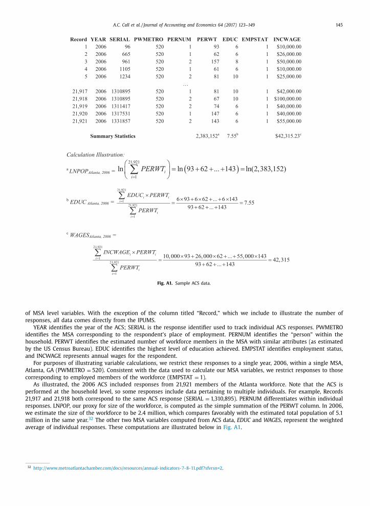
A.C. Call et al. / Journal of Accounting and Economics 64 (2017) 123–149 145

Fig. A1. Sample ACS data.

of MSA level variables. With the exception of the column titled “Record,” which we include to illustrate the number of

responses, all data comes directly from the IPUMS.

YEAR identifies the year of the ACS; SERIAL is the response identifier used to track individual ACS responses. PWMETRO

identifies the MSA corresponding to the respondent’s place of employment. PERNUM identifies the “person” within the

household. PERWT identifies the estimated number of workforce members in the MSA with similar attributes (as estimated

by the US Census Bureau). EDUC identifies the highest level of education achieved. EMPSTAT identifies employment status,

and INCWAGE represents annual wages for the respondent.

For purposes of illustrating variable calculations, we restrict these responses to a single year, 2006, within a single MSA,

Atlanta, GA (PWMETRO = 520). Consistent with the data used to calculate our MSA variables, we restrict responses to those

corresponding to employed members of the workforce (EMPSTAT = 1).

As illustrated, the 2006 ACS included responses from 21,921 members of the Atlanta workforce. Note that the ACS is

performed at the household level, so some responses include data pertaining to multiple individuals. For example, Records

21,917 and 21,918 both correspond to the same ACS response (SERIAL = 1,310,895). PERNUM differentiates within individual

responses. LN POP , our proxy for size of the workforce, is computed as the simple summation of the PERWT column. In 2006,

we estimate the size of the workforce to be 2.4 million, which compares favorably with the estimated total population of 5.1

million in the same year. 32 The other two MSA variables computed from ACS data, EDUC and WAGES , represent the weighted

average of individual responses. These computations are illustrated below in Fig. A1 .

32 http://www.metroatlantachamber.com/docs/resources/annual-indicators-7-8-11.pdf?sfvrsn=2 .

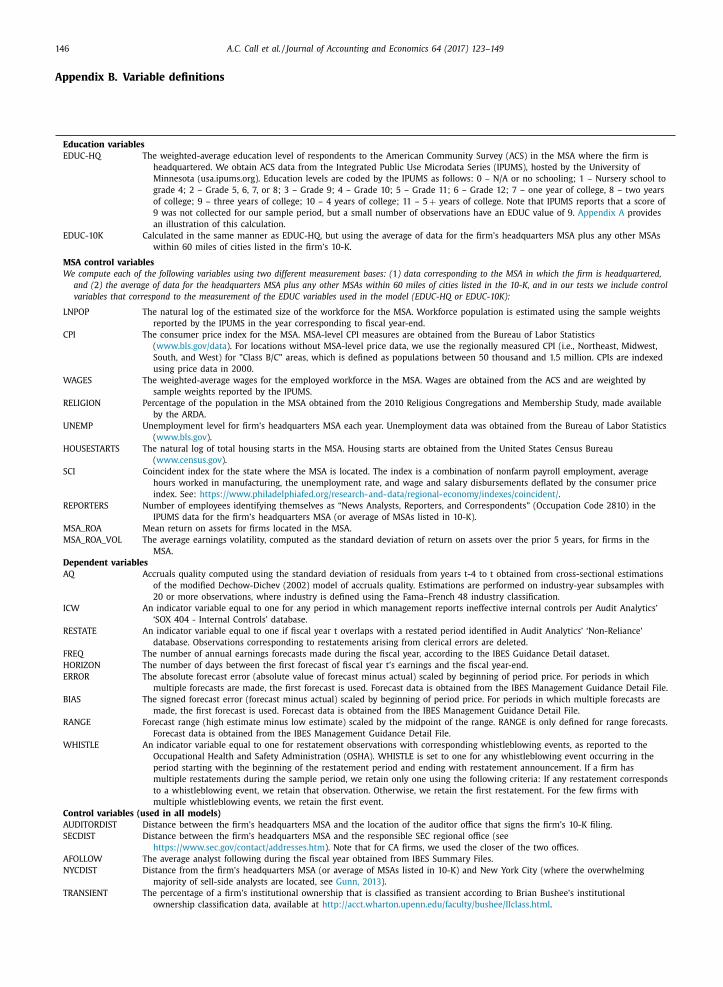
146 A.C. Call et al. / Journal of Accounting and Economics 64 (2017) 123–149

Appe ndix B. Variable definitions

Education variables

EDUC-HQ The weighted-average education level of respondents to the American Community Survey (ACS) in the MSA where the firm is

headquartered. We obtain ACS data from the Integrated Public Use Microdata Series (IPUMS), hosted by the University of

Minnesota (usa.ipums.org). Education levels are coded by the IPUMS as follows: 0 – N/A or no schooling; 1 – Nursery school to

grade 4; 2 – Grade 5, 6, 7, or 8; 3 – Grade 9; 4 – Grade 10; 5 – Grade 11; 6 – Grade 12; 7 – one year of college, 8 – two years

of college; 9 – three years of college; 10 – 4 years of college; 11 – 5 + years of college. Note that IPUMS reports that a score of

9 was not collected for our sample period, but a small number of observations have an EDUC value of 9. Appendix A provides

an illustration of this calculation.

EDUC-10K Calculated in the same manner as EDUC-HQ, but using the average of data for the firm’s headquarters MSA plus any other MSAs

within 60 miles of cities listed in the firm’s 10-K.

MSA control variables

We compute each of the following variables using two different measurement bases: ( 1 ) data corresponding to the MSA in which the firm is headquartered,

and ( 2 ) the average of data for the headquarters MSA plus any other MSAs within 60 miles of cities listed in the 10-K, and in our tests we include control

variables that correspond to the measurement of the EDUC variables used in the model (EDUC-HQ or EDUC-10K):

LNPOP The natural log of the estimated size of the workforce for the MSA. Workforce population is estimated using the sample weights

reported by the IPUMS in the year corresponding to fiscal year-end.

CPI The consumer price index for the MSA. MSA-level CPI measures are obtained from the Bureau of Labor Statistics

( www.bls.gov/data ). For locations without MSA-level price data, we use the regionally measured CPI (i.e., Northeast, Midwest,

South, and West) for "Class B/C" areas, which is defined as populations between 50 thousand and 1.5 million. CPIs are indexed

using price data in 20 0 0.

WAGES The weighted-average wages for the employed workforce in the MSA. Wages are obtained from the ACS and are weighted by

sample weights reported by the IPUMS.

RELIGION Percentage of the population in the MSA obtained from the 2010 Religious Congregations and Membership Study, made available

by the ARDA.

UNEMP Unemployment level for firm’s headquarters MSA each year. Unemployment data was obtained from the Bureau of Labor Statistics

( www.bls.gov ).

HOUSESTARTS The natural log of total housing starts in the MSA. Housing starts are obtained from the United States Census Bureau

( www.census.gov ).

SCI Coincident index for the state where the MSA is located. The index is a combination of nonfarm payroll employment, average

hours worked in manufacturing, the unemployment rate, and wage and salary disbursements deflated by the consumer price

index. See: https://www.philadelphiafed.org/research- and- data/regional- economy/indexes/coincident/ .

REPORTERS Number of employees identifying themselves as “News Analysts, Reporters, and Correspondents” (Occupation Code 2810) in the

IPUMS data for the firm’s headquarters MSA (or average of MSAs listed in 10-K).

MSA_ROA Mean return on assets for firms located in the MSA.

MSA_ROA_VOL The average earnings volatility, computed as the standard deviation of return on assets over the prior 5 years, for firms in the

MSA.

Dependent variables

AQ Accruals quality computed using the standard deviation of residuals from years t-4 to t obtained from cross-sectional estimations

of the modified Dechow-Dichev (2002) model of accruals quality. Estimations are performed on industry-year subsamples with

20 or more observations, where industry is defined using the Fama–French 48 industry classification.

ICW An indicator variable equal to one for any period in which management reports ineffective internal controls per Audit Analytics’

‘SOX 404 - Internal Controls’ database.

RESTATE An indicator variable equal to one if fiscal year t overlaps with a restated period identified in Audit Analytics’ ‘Non-Reliance’

database. Observations corresponding to restatements arising from clerical errors are deleted.

FREQ The number of annual earnings forecasts made during the fiscal year, according to the IBES Guidance Detail dataset.

HORIZON The number of days between the first forecast of fiscal year t’s earnings and the fiscal year-end.

ERROR The absolute forecast error (absolute value of forecast minus actual) scaled by beginning of period price. For periods in which

multiple forecasts are made, the first forecast is used. Forecast data is obtained from the IBES Management Guidance Detail File.

BIAS The signed forecast error (forecast minus actual) scaled by beginning of period price. For periods in which multiple forecasts are

made, the first forecast is used. Forecast data is obtained from the IBES Management Guidance Detail File.

RANGE Forecast range (high estimate minus low estimate) scaled by the midpoint of the range. RANGE is only defined for range forecasts.

Forecast data is obtained from the IBES Management Guidance Detail File.

WHISTLE An indicator variable equal to one for restatement observations with corresponding whistleblowing events, as reported to the

Occupational Health and Safety Administration (OSHA). WHISTLE is set to one for any whistleblowing event occurring in the

period starting with the beginning of the restatement period and ending with restatement announcement. If a firm has

multiple restatements during the sample period, we retain only one using the following criteria: If any restatement corresponds

to a whistleblowing event, we retain that observation. Otherwise, we retain the first restatement. For the few firms with

multiple whistleblowing events, we retain the first event.

Control variables (used in all models)

AUDITORDIST Distance between the firm’s headquarters MSA and the location of the auditor office that signs the firm’s 10-K filing.

SECDIST Distance between the firm’s headquarters MSA and the responsible SEC regional office (see

https://www.sec.gov/contact/addresses.htm ). Note that for CA firms, we used the closer of the two offices.

AFOLLOW The average analyst following during the fiscal year obtained from IBES Summary Files.

NYCDIST Distance from the firm’s headquarters MSA (or average of MSAs listed in 10-K) and New York City (where the overwhelming

majority of sell-side analysts are located, see Gunn, 2013 ).

TRANSIENT The percentage of a firm’s institutional ownership that is classified as transient according to Brian Bushee’s institutional

ownership classification data, available at http://acct.wharton.upenn.edu/faculty/bushee/IIclass.html .

A.C. Call et al. / Journal of Accounting and Economics 64 (2017) 123–149 147

LOCMONITOR Following Ayers et al. (2011) , the percentage of a firm’s institutional ownership that is ( 1 ) classified as dedicated or quasi-indexer

according to Brian Bushee’s institutional ownership classification data, ( 2 ) ranked in the top 5 of institutional owners by

ownership percentage, and located within 100 km of the firm’s headquarters. We obtain investment bank locations from 13F

filings.

NONLOCMONITOR Following Ayers et al. (2011) , the percentage of a firm’s institutional ownership that is ( 1 ) classified as dedicated or quasi-indexer

according to Brian Bushee’s institutional ownership classification data, ( 2 ) ranked in the top 5 of institutional owners by

ownership percentage, and located more than 100 km from the firm’s headquarters. We obtain investment bank locations from

13F filings.

OTHER Institutional ownership percentage not classified as TRANSIENT, LOCMONITOR, or NONLOCALMONITOR.

BOARDEDUC The average education level of all executives and directors listed in BoardEx. We assign education values as follows: 0 = Less than

an Associates degree; 1 = Associates degree; 2 = Bachelors degree; 3 = Masters degree; 4 = higher than Masters (e.g., JD, PhD,

MD). BoardEx sometimes provides somewhat vague education levels, such as “advanced degree,” which we consider to be a

master’s degree, or “degree,” “diploma,” or “graduated,” which we consider to be a bachelor’s degree. If the company does not

appear in BoardEx, we assign a value of 0 to BOARDEDUC.

MISSING_BX An indicator equaling 1 if the observation is missing BoardEx data.

Control Variables (used in select models)

AGE The natural log of the number of years the firm appears in CRSP. When ICW or RESTATE (WHISTLE) is the dependent variable,

AGE is measured as of the current fiscal year (beginning of the restatement period).

AGLOSS An indicator variable equal to one for firms in which earnings (Compustat IB) in t-1 and t sum to less than 0.

BETA Beta, obtained from firm-specific regressions of daily returns on CRSP value-weighted market return over fiscal year prior to

forecast.

BIG4 An indicator variable equal to one if the firm-year audited is by a Big 4 auditor according to Compustat (data item AU).

BTM The book value of equity (Compustat SEQ) divided by the market value of equity (Compustat PRCC_F multiplied by CSHO).

CAP_INT The intensity of capital assets, defined as Net Property, Plant, and Equipment (Compustat PPENT) divided by total assets.

CFVOL The volatility of operating cash flows (Compustat OANCF) from t-4 to t scaled by assets (Compustat AT).

DISPERSION The standard deviation of analyst estimates. For OCCUR and FREQ, DISPERSION is measured as of the beginning of the fiscal year.

For all other forecast variables, DISPERSION is measured using the IBES summary report dated closest to but before the

management forecast date.

EARNVOL The standard deviation of earnings (Compustat IB) scaled by assets (Compustat AT) over years t-5 to t-1.

EXTSG An indicator variable equal to one for observations in which year-over-year industry-adjusted sales growth falls in the top quintile.

FOREIGN An indicator variable equal to one for observations with non-zero values for Foreign Currency Translation Adjustments (Compustat

FCA) in year t.

HIGHVOL An indicator variable equal to one for firms in the highest quartile of return volatility, measured using the standard deviation of

daily returns during the year.

IA_ROA The decile ranking of industry-adjusted return on assets (Compustat IB divided by Compustat AT) in fiscal year t. Ranks are scaled

such that they vary between 0 and 1.

IDIOSHOCKS Firm-specific idiosyncratic shocks as defined in Owens et al., (2017) . Specifically, IDIOSHOCKS is measured using the

root-mean-squared-error from regressing monthly returns on the CRSP value-weighted index and a value-weighted

2-digit-SIC-defined industry portfolio over the 24 months concluding at the end of the current fiscal year.

INT_DUM An indicator variable equal to one for firms with missing values for R&D (Compustat XRD) or Advertising (Compustat XAD).

INT_INT The intensity of intangible assets, defined as R&D (Compustat XRD) plus Advertising (Compustat XAD) divided by assets. Missing

values of R&D and advertising are set to 0.

LEV Financial leverage defined as long-term debt (Compustat DLTT) plus debt due within a year (Compustat DD1) scaled by assets

(Compustat AT). When ICW or RESTATE (FREQ, HORIZON, ERROR, BIAS, or RANGE) is the dependent variable, LEV is defined

using data from the current (prior) fiscal year.

LIT An indicator variable equal to one for firms in high-risk litigation industries defined as SIC codes between 2833–2836, 8731–8734,

3570–3577, 7370–7374, 3600–3674, or 5200–5961.

LNASSETS The natural log of assets (Compustat AT) at the end of fiscal year t.

LNMVE The natural log of the market value of equity (Compustat CSHO times PRCC_F). When ICW or RESTATE (FREQ, HORIZON, ERROR,

BIAS, or RANGE) is the dependent variable, LNMVE is defined using data from the current (prior) fiscal year.

LNOPCYCLE The natural log of the firm’s operating cycle in period t, defined as 360 divided by the ratio of sales (Compustat SALE) to average

accounts receivable (Compustat RECT) plus 360 divided by the ratio of Cost of Goods Sold (Compustat COGS) divided by average

inventory (Compustat INVT).

LNSEG The natural log of the sum of operating and geographic segments reported in Compustat’s Historical Segments file in fiscal year t.

LOSS An indicator variable equal to one for firms reporting negative earnings (Compustat IB) in year t.

MEANTURN The average daily volume divided by shares outstanding over the fiscal year.

MERGE_ACQ An indicator variable equal to one for observations with non-zero, non-missing cash flows related to acquisitons (Compustat AQP).

NLOSSES The number of years between t-4 and t in which the firm reports negative earnings (Compustat IB).

PEERSHOCKS The mean value of IDIOSHOCKS for year t for firms in the same 2-digit SIC code as firm i.

RESTRUCT An indicator variable equal to one for observations in which restructuring charges (Compustat RCP) is greater than 0.

RETVOL The standard deviation of daily returns over the fiscal year.

SALEVOL The volatility of sales (Compustat SALE) from t-4 to t scaled by assets (Compustat AT).

SURPRISE The absolute value of the difference between the forecast and mean analyst forecast from I/B/E/S immediately preceding the

estimate.

ZSCORE The Altman Z-score computed as the inverse cumulative density function of −4.3–4.5 ∗ROA + 5.7 ∗Lev-0.004 ∗Current, where ROA is

Compustat IB divided by Compustat AT, Lev is Compustat LT divided by Compustat AT, and Current is Compustat ACT divided by

Compustat LCT.

�EARN The change in earnings (Compustat IB) from t-1 to t scaled by beginning of period assets (Compustat AT).

148 A.C. Call et al. / Journal of Accounting and Economics 64 (2017) 123–149

Whistleblowing control variables (if not defined previously)

DURATION The number of days between the start and end of the restatement period divided by 365.

DOWNSIZE The mean growth in employees (Compustat EMP) in the three years prior to the restatement period. For periods lacking two

consecutive years of data needed to compute the change, the percentage change is set to 0.

ICW_RISK The risk of an internal control weakness, using the model and reported coefficients from Doyle et al., (2007) . Specifically, we

generate fitted values from −2.182 - 0.80 ∗SIZE - 0.136 ∗AGE + 0.438 ∗AGLOSS + 0.269 ∗LNSEG + 0.311 ∗FOREIGN + 0.227 ∗EXTSG

+ 1.184 ∗RESTRUCT. All variables are defined above and are measured in the period immediately preceding the start of the

restatement period.

LNSALES The natural log of sales (Compustat SALE) in the period immediately preceding the start of the restatement period.

LNSG The natural log of one plus the percentage sales growth (Compustat SALE) in the period immediately preceding the restatement

period.

RETURNS The 12-month buy-and-hold stock return immediately preceding the start of the restatement period.

QUITAM An indicator variable equal to one for observations in two-digit SIC 80 (Healthcare) or listed in the Department of Defense’s "100

Companies Receiving the Largest Dollar Volume of Prime Award Contracts" in any of the three years prior to the restatement

period.

RD_SALES The ratio of R&D (Compustat XRD) to Sales (Compustat SALE) in the period immediately preceding the start of the restatement

period.

REPUTATION An indicator variable equal to one for any firms recognized in Fortune magazine’s “Most Admired” or “Best Place to Work for” lists

in the 5 years prior to the restatement period.

References

Aier, J.K. , Comprix, J. , Gunlock, M.T. , Lee, D. , 2005. The financial expertise of CFOs and accounting restatements. Account. Horiz. 19 (3), 123–135 . Ajinkya, B. , Bhojraj, S. , Sengupta, P. , 2005. The association between outside directors, institutional investors and the properties of management earnings

forecasts. J. Account. Res. 43 (3), 343–376 .

Ayers, B. , Ramalingegowda, S. , Yeung, E. , 2011. Hometown advantage: the effects of monitoring institution location on financial reporting discretion. J.Account. Econ. 52 (1), 41–61 .

Ball, R. , Jayaraman, S. , Shivakumar, L. , 2012. Audited financial reporting and voluntary disclosure as complements: a test of the confirmation Hypothesis. J.Account. Econ. 53 (1-2), 136–166 .

Baik, B. , Farber, D. , Lee, S. , 2011. CEO ability and management earnings forecasts. Contemporary Account. Res. 28 (5), 1645–1668 . Bamber, L. , Jiang, J. , Wang, I. , 2010. What’s my style? The influence of top managers on voluntary corporate financial disclosure. Account. Rev. 85 (4),

1131–1162 .

Bamber, L. , Hui, K.W. , Yeung, E. , 2010. Managers’ eps forecasts: nickeling and diming the market. Account. Rev. 85 (1), 63–95 . Beck, M.J. , Francis , Gunn, J. , 2017. Public Company Audits and City-Specific Labor Characteristics. Contemporary Accounting Research conditionally accepted .

Bergstresser, D. , Philippon, T. , 2006. CEO incentives and earnings management. J. Financ. Econ. 80 (3), 511–529 . Bernile, G. , Kumar, A. , Sulaeman, J. , 2015. Home away from home: Geography of information and local investors. Rev. Financ. Stud. 28 (7), 2009–2049 .

Bowen, R. , Call, A. , Rajgopal, S. , 2010. Whistle-blowing: target firm characteristics and economic consequences. Account. Rev. 85 (4), 1239–1271 . Call, A. , Kedia, S. , Rajgopal, S. , 2016. Rank and File employees and the discovery of misreporting: the role of stock options. J. Account. Econ. 62 (2), 277–300 .

Call, A. , Martin, G. , Sharp, N. , Wilde, J. , 2017. Whistleblowers and outcomes of financial misrepresentation enforcement actions. J. Account. Res. In-press . Cassell, C. , Dreher, L. , Myers, L. , 2013. Reviewing the SEC’s review process: 10-K comment letters and the cost of remediation. Account. Rev. 88 (6),

1875–1908 .

Chen, S. , 2004. Why do managers fail to meet their own forecasts?. University of Texas Working Paper . Cheng, M. , Dhaliwal, D. , Zhang, Y. , 2013. Does investment efficiency improve after the disclosure of material weaknesses in internal control over financial

reporting. J. Account. Econ. 56 (1), 1–18 . Cheng, Q. , Warfield, T.D. , 2005. Equity incentives and earnings management. Account. Rev. 80 (2), 441–476 .

Choi, J.-H. , Kim, K.-B. , Qiu, A. , Zang, Y. , 2012. Geographic proximity between auditor and client: How does it impact audit quality? A J. Pract. Theor. 31 (2),43–72 .

Chyz, J. , 2013. Personally tax aggressive executives and corporate tax sheltering. J. Account. Econ. 56 (2-3), 311–328 .

Dorantes, C.A. , Li, C. , Peters, G.F. , Richardson, V.F. , 2013. The effect of enterprise systems implementation on the firm information environment. Contemp.Account. Res. 30 (4), 1427–1461 .

Dechow, P.M. , Dichev, I.D. , 2002. The quality of accruals and earnings: the role of accrual estimation errors. Account. Rev. 77 (s-1), 35–59 . Demerjian, P. , Lev, B. , Lewis, M. , McVay, S. , 2013. Managerial ability and earnings quality. Account. Rev. 88 (2), 463–498 .

Dhaliwal, D. , Erickson, M. , Heitzman, S. , 2009. Taxes and backdating of stock option exercises. J. Account. Econ. 47, 27–49 . Doyle, J. , Ge, W. , McVay, S. , 2007. Determinants of weaknesses in internal control over financial reporting. J. Account. Econ. 44 (1–2), 193–223 Conference

Issue on Corporate Governance: Financial Reporting, Internal Control, and Auditing: .

Dyck, A. , Morse, A. , Zingales, L. , 2010. Who blows the whistle on corporate fraud. J. Finance 65 (6), 2213–2253 . Dyreng, S.D. , Hanlon, M. , Maydew, E.L. , 2010. The effects of executives on corporate tax avoidance. Account. Rev. 85 (4), 1163–1189 .

Dyreng, S. , Mayew, W. , Williams, C. , 2012. Religious social norms and corporate financial reporting. J. Bus. Finance Account. 39 (7-8), 845–875 . Francis, J. , LaFond, R. , Olsson, P. , Schipper, K. , 2004. Costs of equity and earnings attributes. Account. Rev. 79 (4), 967–1010 .

Francis, J. , Nanda, D. , Olsson, P. , 2008. Voluntary disclosure, earnings quality, and cost of capital. J. Account. Res. 46 (1), 53–99 . Francis, J. , Maydew, E. , Sparks, H.C. , 1999. The role of big 6 auditors in the credible reporting of accruals. Account. Rev. 18 (2), 17–34 .

Feng, M. , Ge, W. , Luo, S. , Shevlin, T. , 2011. Why do CFOs become involved in material accounting manipulations. J. Account. Econ. 51 (1–2), 21–36 .

Feng, M. , Li, C. , McVay, S. , 2009. Internal control and management guidance. J. Account. Econ. 48 (2), 190–209 . Garcia, D. , Norli, O. , 2012. Geographic dispersion and stock returns. J. Financial Econ. 106 (3), 547–565 .

Ge, W. , Matsumoto, D. , Zhang, J.L. , 2011. Do CFOs have style? An empirical investigation of the effect of individual CFOs on accounting practices. Contemp.Account. Res. 28 (4), 1141–1179 .

Ghoshal, S. , 2005. Bad management theories are destroying good management practices. Acad. Manag. Learn. Educ. 4 (1), 75–91 . Gintis, H. , Khurana, R. , 2008. Corporate honesty and business education: A behavioral model. In: Zak, P. (Ed.), Moral Markets: The Critical Role of Values in

the Economy. Princeton University Press, Princeton, NJ, pp. 300–327 .

Glaeser, E.L. , Saks, R.E. , 2006. Corruption in America. J. Public Econ. 90 (6–7), 1053–1072 . Glaeser, E.L. , Gottlieb, J.D. , 2009. The wealth of cities: agglomeration economies and spatial equilibrium in the United States. J. Econ. Lit. 47 (4), 983–1028 .

Gunn, J. , 2013. City-location and Sell-side Analyst Research. University of Pittsburgh Working Paper . Hambrick, D. , Mason, P. , 1984. Upper echelons: The organization as a reflection of its top managers. Acad. Manage. Rev. 9 (2), 193–206 .

Hennes, K. , Leone, A. , Miller, B. , 2008. The Importance of distinguishing errors from irregularities in restatement research: The case of restatements andCEO/CFO turnover. Account. Rev. 83 (6), 1487–1519 .

A.C. Call et al. / Journal of Accounting and Economics 64 (2017) 123–149 149

Karamanou, I. , Vafeas, N. , 2005. The association between corporate boards, audit committees, and management earnings forecasts: An empirical analysis. J.Account. Res. 43 (3), 453–486 .

Kedia, S. , Rajgopal, S. , 2011. Do the SEC’s enforcement preferences affect corporate misconduct? J. Account. Econ. 51 (3), 259–278 . Lipset, S. , 1960. Political Man: The Social Bases of Politics. Doubleday, Garden City, NY .

McGuire, S.T. , Omer, T.C. , Sharp, N.Y. , 2012. The impact of religion on financial reporting irregularities. Account. Rev. 87 (2), 645–673 . McNichols, M.F. , 2002. Discussion of the quality of accruals and earnings: the role of accrual estimation errors. Account. Rev. 77 (s-1), 61–69 .

Merchant, K.A. , Rockness, J. , 1994. The ethics of managing earnings: an empirical investigation. J. Account. Pub. Policy 13 (1), 79–94 .

Miller, G.S. , 2006. The press as a watchdog for accounting fraud. Account. Rev. 44 (5), 1001–1033 . Moretti, E. , 2004. Chapter 51 Human capital externalities in cities. In: H, J.V., Thisse, J.-F. (Eds.). In: Handbook of Regional and Urban Economics, 4. Elsevier,

pp. 2243–2291. Cities and Geography . O’Fallon, M.J. , Butterfield, K.D. , 2005. A review of the empirical ethical decision-making literature: 1996-2003. J. Bus. Ethics 59 (4), 375–413 .

Owens, E.L. , Wu, J.S. , Zimmerman, J. , 2017. Idiosyncratic shocks to firm underlying economics and abnormal accruals. Account. Rev. 92 (2), 183–219 . Rogers, J. , Stocken, P. , 2005. Credibility of management forecasts. Account. Rev. 80 (4), 1233–1260 .

Ruggles, S. , Alexander, J.T. , Genadek, K. , Goeken, R. , Schroeder, M.B. , Sobek, M. , 2010. Integrated Public Use Microdata Series: Version 5.0 [Machine-readableDatabase]. University of Minnesota, Minneapolis .

Waymire, G. , 1985. Earnings volatility and voluntary management forecast disclosure. J. Account. Res. 23 (1), 268–295 .

Wilde, J. , 2017. The deterrent effect of employee whistleblowing on firms’ financial misreporting and tax aggressiveness. Account. Rev. In-press . Yu, F.F. , 2008. Analyst coverage and earnings management. J. Financ. Econ. 88 (2), 245–271 .