Journal of Advances in Mechanical Engineering and Science ... · PDF fileOptimal Fixture Design for Drilling of Elastomer using DOE and ... Taguchi’s approach to design of experiments

Journal of Advances in Mechanical Engineering and Science, Vol. 2(2) 2016, pp. 1-19

*Corresponding author. Tel.: +919842960609

Email address: [email protected] (S.Selvakumar)

Double blind peer review under responsibility of DJ Publications

http://dx.doi.org/10.18831/james.in/2016021001

2455-0957 © 2016 DJ Publications by Dedicated Juncture Researcher’s Association. This is an open access

article under the CC BY-NC-ND license (http://creativecommons.org/licenses/by-ncnd/4.0/) 1

RESEARCH ARTICLE

Optimal Fixture Design for Drilling of Elastomer using DOE and FEM

*S Selvakumar

1, K.M Arunraja

2, P Praveen

3

1Assistant Professor (SLG), Department of Mechanical Engineering, Kongu Engineering College,

Perundurai – 638052, Tamil Nadu, India. 2Assistant Professor, Department of Mechanical Engineering, Hindusthan Institute of Technology,

Coimbatore-641032, Tamil Nadu, India. 3Assistant Professor, Department of Mechanical Engineering, Excel Engineering College, Sankari

west – 637303, Tamil Nadu, India.

Received-18 January 2016, Revised-14 March 2016, Accepted-16 March 2016, Published-22 March 2016

ABSTRACT

An elastomer is a polymer with the property of viscoelasticity generally having notably low

Young's modulus and high yield strain compared with other materials. The elastomer which is used in

our project is styrene-butadiene rubber. The drilling of elastomer work piece is not easy since it can

easily deform. Hence the desired output cannot be obtained. By designing a proper fixture layout, the

drilling of elastomer can be done accurately. The fixture design requires accurate positioning of

locators and clamps to reduce the deformation of work piece during drilling. In this work six locators

and three clamps are used. The primary design layout is done and then it is analyzed in ANSYS to find

out the work piece deformation. The various possible design layouts are formed using L27 orthogonal

array by MINITAB Software. Then all the 27 layouts are analyzed using ANSYS and the deformation

values are found. The optimal layout is found using DOE – Taguchi method from MINITAB Software

by giving the 27 layouts and the corresponding deformation values as inputs. From the obtained SN

ratio graph, the optimal fixture layout is found for minimum deformation of the work piece.

Keywords: Elastomer, Styrene-butadiene rubber, Drilling, Deformation, Polymerization.

1. INTRODUCTION

The fixture developing includes

placing the locators and clamps in correct

positions according to the material selected.

Here we will see about the material selected

and the various components of fixtures and its

types.

1.1. Elastomer and it’s use

An elastomer is a polymer with the

property of viscoelasticity generally having

notably low Young's modulus and high yield

strain compared with other materials. Each of

the monomers which link to form the polymer

is usually made

of carbon, hydrogen, oxygen and/or silicon.

Elastomers are amorphous polymers

existing above their glass transition

temperature, so that considerable segmental

motion is possible. At ambient temperatures,

rubbers are thus relatively soft and deformable.

Their primary uses are for seals, adhesives and

moulded flexible parts. The elastomer used in

our project is styrene-butadiene rubber.

Styrene butadiene rubber is a synthetic

rubber copolymer consisting of styrene and

butadiene. It has good abrasion resistance and

good aging stability when protected by

additives, and is widely used in car tires, where

it may be blended with natural rubber. It was

originally developed prior to World War II in

Germany.

SBR can be produced by two basically

different processes: from solution or as

emulsion. In the first instance the reaction is

ionic polymerization. In the emulsion

polymerization case the reaction is via free

radical polymerization. In this process, low

pressure reaction vessels are required and

usually charged with styrene and butadiene,

two monomers, a free radical generator and a

http://www.djjames.in/




S.Selvakumar et al./Journal of Advances in Mechanical Engineering and Science, Vol. 2(2), 2016 pp. 1-19

2

chain transfer agent such as an alkyl mercaptan

and water. Mercaptans control molecular

weight and the high viscosity product from

forming. The anionic polymerization process is

initiated by alkyl lithium and water which is

not involved. High styrene content rubbers are

harder but less rubbery.

The elastomer is used widely in

pneumatic tires, shoe heels, soles, gaskets etc.

It is a commodity material which competes

with natural rubber. Latex SBR is extensively

used in coated papers, being one of the most

cost-effective resins to bind pigmented

coatings. It is also used in building applications

as a sealing and binding agent behind renders

as an alternative to PVA, but is more

expensive. In the latter application, it offers

better durability, reduced shrinkage and

increased flexibility, as well as resistance to

emulsification in damp conditions. SBR can be

used to 'tank' damp rooms or surfaces, a

process in which the rubber is painted onto the

entire surface forming a continuous, seamless

damp proof liner.

1.2. Fixture and its types

A fixture is a work-holding or support

device used in the manufacturing industry. The

main purpose of a fixture is to locate and hold

a work piece during a machining operation.

Fixtures are normally designed for a definite

operation to process a specific work piece and

are designed and manufactured individually.

The typical fixture elements are the locating

device, clamping device and base plate.

1.2.1. Types of fixtures

There are many types of fixtures such

as plate fixture, angle-plate fixture, vise-jaw

fixture, indexing fixture, multi station fixture

and profiling fixture. These fixtures are used

for various operations like drilling, honing,

assembling, boring, reaming, inspecting, heat

treating, tapping, testing, etc.

1.3. DOE – Taguchi technique

MINITAB is a powerful statistical

software program that provides a wide range of

basic and advanced capabilities for statistical

analysis. It works with data in the form of rows

and columns. MINITAB has many statistical

analyses such as ANOVAs, DOE, control

charts, quality tools, etc. In our project we use

DOE-Taguchi 3 level as an optimization tool.

The orthogonal array chosen here is L27

corresponding to number of parameters as 9.

Taguchi’s techniques have been used

widely in engineering design. The main trust of

Taguchi’s techniques is the use of parameter

design, which is an engineering method for

product or process design that focuses on

determining the parameter settings producing

the best levels of a quality characteristic with

minimum variation. To determine the best

design, it requires the use of a strategically

designed experiment, which exposes the

process to various levels of design parameters.

Taguchi’s approach to design of experiments is

easy to be adopted and applied for users with

limited knowledge of statistics; hence it has

gained a wide popularity in the engineering

and scientific community. Further, depending

on the number of factors, interactions and their

level, an orthogonal array is selected by the

user. Taguchi has used signal–noise ratio as the

quality characteristic of choice. S/N ratio is

used as measurable value instead of standard

deviation due to the fact that, as the mean

decreases, the standard deviation also deceases

and vice versa. In other words, the standard

deviation cannot be minimized first and the

means brought to the target two of the

applications in which the concept of S/N ratio

is useful are the improvement of quality

through variability reduction and the

improvement of measurement. The S/N ratio

characteristics can be divided into three

categories, when the characteristic is

continuous. Nominal and smaller are the best

and larger is better. Here we use smaller as the

better option for optimization.

2. LITERATURE REVIEW

This chapter deals with the various

journals and articles referred, to design the

fixture layout for drilling of the elastomer. The

journals are referred, to find out the properties

of elastomer and optimal fixture design layout

for drilling of work pieces. The journals and

their important points are described here.

2.1. Fixture design for drilling through

deformable plate work pieces - Part I

[1] In this study, the method of finite

elements is employed for the purpose of

calculating the workpiece deformations

induced by the drilling loads. It is understood

that the actual drilling process may be governed

by nonlinear interactions between the penetrating


3

drill and the deforming work piece. For

example, the removal of material during

drilling alters the geometry and thus the

structural stiffness of the work piece, which in

turn leads to higher deformations, both in the

near-drill proximity as well as in remote regions

of the work piece. In addition to the local and

global effects of material removal, nonlinear

damage evolution in the near- drill proximity is

also expected to augment the local deformation

field, which determines the quality of the

drilling process. This may include several types

of damage such as micro cracking in ceramics,

delamination in composite laminates, plasticity

in metals, fiber de-bonding and pull-out in

fibre reinforced composites and other potential

forms of damage. To account for all of the

above, a robust nonlinear finite element model

needs to be developed. Such a nonlinear and

computationally intensive model will then need

to be embedded within an iterative optimization

scheme. This optimization scheme is designed

to assess the quality of the drilling process with

built-in capabilities of identifying optimal

restraining fixture configurations. While such a

far-reaching modelling objective is now being

considered, in this study we adopt a rather

simplistic approach in simulating the drilling

process using the method of finite elements.

The boundary value problem and the

assumptions used in the development of the

finite element model in this study are presented

next.

As discussed earlier in this work,

the drilling process is a highly nonlinear

phenomenon governed by material,

geometric and contact nonlinearities[2]. To

accurately simulate such a process, one needs

to employ an incremental f inite element

scheme embedded in an iterative

optimization algorithm. Thus, tens or

possibly hundreds of thousands of finite

element incremental solutions are required

to be completed in conducting optimal drilling

simulations. While such a task may be

computationally feasible for future studies,

in this work it was sought to derive useful

insights on optimal fixturing by simulating

drilling as a linear process.

[3]More specifically, it is assumed that

no damage of any form develops during

drilling. It is assumed that the contact between

the drill bit and the elastically deforming plate

gives rise to constant drilling loads, which are

modelled as a drilling concentrated thrust, FZ

and a line-distributed drilling torque,

M. Consequently, the material is removed in

one step, greatly reducing the needed

computations. As such, the drilling process is

simulated by considering a preexisting

terminal cylindrical hole in the plate of

diameter equal to that of the drill bit. The

drilling thrust and moment developed at the

leading front of the drilling process are thus

introduced as applied loads acting on the

bottom surface of the hole, as shown

schematically in figure B1. In the simulations

reported here, a hole depth was selected to be

equal to 0.9h throughout the study. This

selection was based on solution convergence

studies wherein the radial displacement

component at the rim of the hole was

monitored as a function of the hole depth. One

may argue that modelling the drilling process

using a preexisting hole reduces the overall

stiffness of the work piece, which also

introduces inaccuracies. It is important to state

that in developing the current one- step drilling

model, the above issue was considered and

found to be irrelevant because at the end of the

drilling process one encounters a weakened

work piece that is consistent with the current

preexisting hole model.

2.2. Fixture design for drilling through

deformable plate work pieces - Part II

[4] The finite element fixturing

modelling, together with the material removal

tools developed and the objective function

analysis addressed in Part I, form the

optimal fixturing model for drilling

through plate deformable work pieces. The

computer simulations presented in this

section have been conducted with the aid

of the optimal fixturing model. Before

presenting the specifics of the simulations

discussed in this section, it may be of

importance to note that each simulation

involves one of the above five objective

functions as proposed in Part I and is

conducted under a rather demanding iterative

computational scheme. For example, the

elastic plate is initially constrained

consistently with the loading and

geometric boundary conditions shown

in Part I. The associated boundary value

problem put forth is then solved using the

ABAQUS FE software. The 3-D finite

element solution is then used to extract

the pertinent information regarding the


4

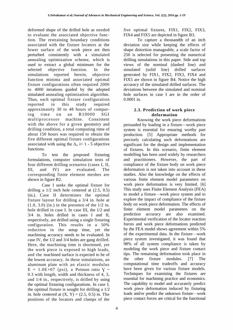
deformed shape of the drilled hole as needed

to evaluate the associated objective func-

tion. The restraining boundary conditions

associated with the fixture locators at the

lower surface of the work piece are then

perturbed consistently with a simulated

annealing optimization scheme, which is

used to extract a global minimum for the

selected objective function. In the

simulations reported herein, objective

function minima and associated optimal

fixture configurations often required 2000

to 4000 iterations guided by the adopted

simulated annealing optimization algorithm.

Thus, each optimal fixture configuration

reported in this study required

approximately 30 to 48 hours of comput-

ing t im e on an R10000 SGI

mul t ip rocessor machine. Consistent

with the above for a given geometry and

drilling condition, a total computing time of

about 150 hours was required to obtain the

five different optimal fixture configurations

associated with using the Δi, i= 1 - 5 objective

functions.

To test the proposed fixturing

formulations, computer simulation tests of

four different drilling scenarios (cases I, II,

III, and IV) are evaluated. The

corresponding finite element meshes are

shown in figure B2.

Case I seeks the optimal fixture for

drilling a 1/2 inch hole centered at (2.5, 0.5)

(in.). Case II determines the optimal

fixture layout for drilling a 3/4 in. hole at

(1.0, 3.0) (in.) in the presence of the 1/2 in.

hole drilled in case I. In case III, the 1/2 and

3/4 in. holes drilled in cases I and II,

respectively, are drilled using a single fixturing

configuration. This results in a 50%

reduction in the setup time, yet the

machining accuracy needs to be evaluated. In

case IV, the 1/2 and 3/4 holes are gang drilled.

Here, the machining time is shortened, yet

the work piece is exposed to high loads,

and the machined surface is expected to be of

the lowest accuracy. In these simulations, an

aluminum plate with an elastic modulus

E = 1.0E+07 (psi), a Poisson ratio Ɣ =

0.3 with length, width and thickness of 4, 3,

and 1/4 in., respectively, is drilled by using

the optimal fixturing configurations. In case I,

the optimal fixture is sought for drilling a 1/2

in. hole centered at (X, Y) = (2.5, 0.5) in. The

positions of the locators and clamps of the

five optimal fixtures, FIX1, FIX2, FIX3,

FIX4 and FIX5 are depicted in figure B3.

To capture a thousandth of an inch

deviation size while keeping the effects of

shape distortion manageable, a scale factor of

250 is selected for presenting the numerical

drilling simulations in this paper. Side and top

views of the nominal (dashed line) and

simulated (solid line) drilled surfaces

generated by FIX1, FIX2, FIX3, FIX4 and

FIX5 are shown in figure B4. Notice the high

accuracy of the simulated drilled surfaces. The

deviations between the simulated and nominal

hole surfaces in case I are in the order of

0.0001 in.

2.3. Prediction of work piece

deformation

Knowing the work piece deformations

persuaded by loading in a fixture—work piece

system is essential for ensuring worthy part

production. [5] Appropriate methods for

precisely calculating such deformations are

significant for the design and implementation

of fixtures. In this scenario, finite element

modelling has been used widely by researchers

and practitioners. However, the part of

compliance of the fixture body on work piece

deformation is not taken into account in these

studies. Also the knowledge on the effects of

various finite element model parameters on

work piece deformation is very limited. [6]

This study uses Finite Element Analysis (FEA)

to model a fixture—work piece system and to

explore the impact of compliance of the fixture

body on work piece deformation. The effects of

finite element model parameters on the

prediction accuracy are also examined.

Experimental verification of the locator reaction

forces and work piece deformations predicted

by the FEA model shows agreement within 5%

of the experimental data. In the fixture—work

piece system investigated, it was found that

98% of all system compliance is taken by

modeling the work piece and fixture contact

tips. The remaining deformation took place in

the other fixture modules. [7] The

computational time tradeoffs and accuracy

have been given for various fixture models.

Techniques for examining the fixtures are

essential for machining practice and economics.

The capability to model and accurately predict

work piece deformation induced by fixturing

loads and/or predict the unknown fixture—work

piece contact forces are critical for the functional


5

fixture design. [8] The contact mechanics based

approach, the rigid body approach and the finite

element modelling approach are the approaches

used extensively for fixture—work piece

systems. Among these methods, the rigid body

modelling approach is incapable of predicting

work piece deformations. It is therefore

unsuitable for the study on the influence of

fixturing on part quality. Though the contact

mechanics approach is striking from an angle

of computational effort, it is restricted to parts

that can be estimated as elastic half-spaces.

[9, 10] The fixture-work piece

system used in this study comprised of a

hollow block of rectangular section and

uniform wall thickness with a 3-2-1 fixture

layout as shown in figure B5. The aluminum

6061-T6 (E= 70GPa, v= 0.334) work piece

measured 153 mm X 127 mm X 76 mm and

had a fixed wall thickness (t in figure B1)

ranging from 6 to 10 mm. Two clamps were

used to press the work piece against six

locators: three on the primary plane, two on the

secondary plane, and one on the tertiary

plane. Spherical and planar hardened AISI

1144 steel (E= 206 GPa, v= 0.296) fixture

tips with black oxide finish were used to

locate and clamp the work piece.

While some published literature

including [11, 12, 13, 14] use FEA to study

work piece deformation, a rigorous

examination of the effect of mesh density on

the modelling of fixture work piece

compliance is vague. A vital factor in

determining the suitable FEA model for this

investigation is the selection of ideal mesh

density. A coarse mesh might yield

inaccurate outcomes. On the other hand too

fine a mesh might be unnecessary and

computationally expensive. In this study, the

SMRT smart-meshing function of ANSYS was

utilized to build the solid mesh. Discrete values

ranging from 1 (most dense mesh) to 10

(least dense mesh) were assigned to the

various solid parts. Wide spectrums of

combinations of fixture and work piece mesh

sizes were used to find the optimal mesh size.

To check the accuracy of the results, the

deformation of the work piece, đc1 and

đc2, at the location of the two clamps were

computed.

Experimental results were used as

a benchmark for evaluating the validity of the

simulated results. A test fixture with

dimensions similar to the models was

constructed. The work piece for this study had

a uniform wall thickness of 7 mm. The

fixture elements were secured to a 15 mm

thick steel base plate. The threaded fixture

tips on the primary plane were screwed

directly into the base plate. The other locators

were screwed into steel support blocks that

were in turn each fastened to the base plate

via four bolts and two press-fit dowel pins.

The two clamps, which were

similarly fastened to the base plate via steel

support blocks, were actuated by a hydraulic

hand pump. The order of clamp actuation can

influence work piece deflection as shown by

other researchers and previous works. In the

current study, the two clamps were actuated

simultaneously by a single hydraulic pump.

The difference in actuation times for the two

clamps was deemed to be negligible. The

deformation at each point was measured

using an eddy current proximity probe.

The change in magnetic flux of a target patch

identified by the sensor was converted to a

displacement value by the data acquisition

system. Average deformation results over five

trials for each tip and load pair are taken.

3. PROBLEM DEFINITION

Elastomers, also recognized as

rubbers, are long-chain polymers which unveil

different material properties. They are unique

and the parts of the elastomer are manufactured

by the process of moulding. Raw polymeric

materials are mixed with different additives,

heated, melted and pressed into the shape of a

mould in the moulding process. The polymer

material is then exposed to a controlled

temperature-pressure-time cycle within the

mould. The material is cured, vulcanized, and

cooled to get the anticipated properties and

geometry. A set of moulds is required to

fabricate elastomer parts with complex shapes

such as tire and footwear tread patterns.

Production of these moulds is costly and

consumes more time. It is for these reasons,

machining is regarded as an alternative for

engineering custom and prototype elastomer

machineries [15].

Normally cryogenic machining is

used for elastomers but it has the following

drawbacks,

The work piece requires intensive

care. Since the material is in brittle

form, it can easily break.

High setup time.


6

High operating cost.

Consumes more time for the process

to be completed.

The machining of elastomer work

piece is not easy since it can easily deform and

hence the desired output cannot be obtained.

The optimization of fixture layout is the

process of optimizing the number of fixture

elements such as locators and clamps,

machining force and clamping force. In fixture

design, clamping forces and fixture layout are

the most influencing factors of work piece

deformation. Optimum clamping force and

fixture layout are essential for minimum work

piece deformation.

4. DESIGN AND ANALYSIS OF FIXTURE

DESIGN

The material chosen for our analysis is

styrene-butadiene rubber. The material

properties of the above said material was taken

from the journal papers. The dimension of the

work piece is 100 × 80 × 20mm.The hole is of

25mm diameter and it is drilled centrally [16].

4.1. Proposed design

To overcome these problems, a new

design layout of fixture has been developed.

In this new design layout the locators for the

work piece are placed by 3-2-1 principle. The

clamps were placed opposite to the clamps on

three edges. In this new layout two out of

three locators on the base are fixed very close

to the intended hole position. The design

layout is shown in figure B6. The work piece

dimensions are also shown in the

representation. The design layout is done for

drilling a hole of diameter 25 mm in a

rectangular work piece of 100 mm × 80 mm

× 20 mm. The hole position is the centre of

the work piece. From this design layout,

other possible layouts are formed and

optimized using Taguchi method. The final

optimized design layout will produce less

deformation to the work piece.

4.2. Design of workpiece in ANSYS

In the preprocessor menu of ANSYS

we should select the element type option. As

the element type dialog box opens we can

select the material type. For our project we

chose as solid type and Brick 8node 45.Again

in the preprocessor menu select the modelling

menu. In the modelling menu select create

option. In the create option select rectangle

option. Then create the rectangle by 2 corners

option. As soon as the dialog box appears give

the coordinates for creating the rectangle. The

coordinates are (0,0) and (100,80). For creating

the hole, the cylinder must be created. Go to

create option and select the cylinder option.

Next select the centre & radius option. Then

give the centre point as (50,40) and the radius

as 12.5mm and depth of the cylinder as 20mm.

Select Boolean option from the operations

menu and then select subtract option. Next

select areas from the menu. Then subtract the

cylinder from the rectangular block. Thus the

work piece is created using ANSYS. The

designed work piece is shown in the Figure

4.2.

4.3. Calculation of clamping forces

4.3.1. Power calculation

Material factor, K1 = 0.55

Diameter of drill, d = 25 mm

rpm of drill, n= 1000 rpm

Feed mm/rev, s = 0.25 mm/rev

Drilling power = (1.25xd2x K1xn

(0.056+1.5xs))/105= 2 kW

4.3.2. Force acting on each lip

Specific force, Ks = 650 N/mm2


Feed mm/rev, s = 0.25 mm/rev

Force acting on each lip, P = (Ksxdxs)/4=

1015.6 N

4.3.3. Torque Force acting on each lip, P = 1015.6N


Torque = (Pxd)/20= 1270 Nmm

Thrust Force = Torque/Radius= 101.6 N

4.3.4. Clamping force calculation

Co-efficient of friction, µ = 1.062

By Coulomb’s friction law,

∑ ∑ (4.1)

where L = Locators and

C = Clamping force.

From equation (4.1),

1015.6= (L4 + L5 + L6 + C2 + C3) ×1.062=

(C2 + C3 + C2 + C3) X 1.062

(4.2)

Similarly,

101.6 = (L1 + L2 + L3 + L4 + L5 + C2 + C1)

×1.062= (C1 + C2 + C1 + C2) X 1.062

(4.3)

Assume clamping force, C2 = 25 N

Then from equations (4.2) and (4.3),


7

Clamping force, C1 = 22.8 N

Clamping force, C3 = 453.15 N

4.4. Analysis of fixture layout The first step in the solution part is that

we have to give the material properties of the

work piece. Select the material props option

from the main menu of the preprocessor. Then

select material models option from the material

props menu. Next select the structural option

from the appeared dialog box. Then select

linear option from the menu. Next select the

elastic option. Then select the isotropic option

under the elastic option. Next give the young’s

modulus value as the 10 Mpa. Then give the

Poisson ratio as 0.5.

The second step is the meshing of the

model created. The meshing of the work piece

is done by choosing the meshing option from

the preprocessor menu. First select the mesh

tool option from the meshing menu. In the

mesh tool dialog box set the element attributes

as the global consideration. Then select the

areas option from the mesh menu. Next select

the shape of the mesh. Then select the areas to

be meshed. Finally click on the mesh option on

the mesh tool dialog box.

The third step is the fixing of

constraints i.e., fixing of the locators and the

clamping forces. For our project we chose six

locators as per the 3-2-1 clamping principle.

Then three clamps were used to hold the work

piece tightly in the fixed position. The

clamping forces are calculated according to the

coulomb’s friction law. Then the forces for

drilling operation were also calculated by using

CMTI handbook and HMT machine tools

book. There are two forces acting on the

drilling operation. One force is the thrust force

which is acting downwards along the drill bit.

The second force is the tangential force which

is acting on the side of the hole.

Fourth step is the fixing of the

constraints in the particular position. There are

nine variable parameters to be considered (6

locators and 3 clamps). In order to optimize the

position of the variables we use Taguchi

methodology of optimization. Here we use

Degree of Experiments (DOE). We employ the

help of MINITAB software to obtain the

matrix array. Then the locators and the clamps

are positioned according to the sequence

obtained by the MINITAB software. The

definite range is fixed and the locator positions

and clamping positions are changed according

to the software within the specified range. The

range of the locators and clamping positions

are shown in table A1.

The fifth step is the application of

loads in the determined positions of the

locators and the clamping forces. Then the

tangential force and the thrust force are also

given at a particular point of the hole before

evaluation of the work piece.

The final step is the solving of the

problem. After applying all the constraints and

the clamping forces on the determined

positions, the problem can be solved. For

solving the problem go to the solution

command on the main menu. Then select solve

command from the solution menu. Next solve

current LS option from the solve menu. At last

the solution will be obtained.

After solving the problem we can see

the solution by selecting the general post proc

option from the main menu. In that general

post proc, select the plot results option. In the

plot results dialog box under the DOF option

select displacement vector sum option. Then

select the deformed + undeformed shape

option from the scroll down menu. The

ANSYS screen will show the corresponding

result. Then export the displayed image to the

file. The result taken is shown in the figure B8.

The maximum deformation of the work piece

during the drilling option is noted from the

analysis output. The maximum deformation is

represented as DMX and the contour image

represents the minimum and maximum

deformation.

Now the above said procedures are

repeated for various locator positions and

clamping forces according to the array

obtained from the MINITAB software.

MINITAB is a statistical software program that

provides a wide range of basic and advanced

capabilities for statistical analysis. It works

with data in the form of rows and columns.

After opening MINITAB software click on

stat, select DOE, then select Taguchi to create

a Taguchi design. The type of design in our

optimization is 3-level in which we can use 2

to 13 factors and the number of factors used in

our project is 9. Click on ―display available

design‖ tab to select the correct design for the

optimization. Since 3-level is used, the

available design is L27 orthogonal array.

Now a sequence for L27 orthogonal

array is displayed in the worksheet present at

the bottom of the screen. Each dimension of


8

various locator positions and clamping forces

present in the work piece is divided into 3 so

that the range for each parameter is changed to

take the corresponding results as given in L27

orthogonal array by the MINITAB software.

The work piece deformation for fixture Layout

1 is shown in figure B9.

The deformation results for all the 27

design layouts are obtained. The results are

shown in the table A2.

5. OPTIMIZATION OF FIXTURE

LAYOUT

After taking results for various

sequences of L27 orthogonal array with the

help of ANSYS, the 27 deformation values are

entered in the MINITAB software. Now click

on stat, select DOE, then select Taguchi to

define custom Taguchi design. In the

appearing dialog box, select all the parameters

which are to be present in S/N ratio graph.

Again click on stat, select DOE, then select

Taguchi to analyze Taguchi design. Select the

cell in which response data are present. Click

on graphs tab to generate S/N graph for main

effects and interactions in the model. Next

click on terms tab to select all the available

terms to create S/N ratio graph. Then click on

options tab to select which S/N ratio is to be

chosen. In our optimization method we select

―smaller is the better‖ ratio. Now click on

storage tab to select which data should be

stored after the analysis is done. Then ok

button is clicked. Two dialog boxes will open

showing the S/N graph of main effects in the

model. The S/N graph is shown in figure B10.

From the obtained S/N ratio graph we

can conclude that the effect of changing the

positions of locator 1,2,3,4 and 5 and clamping

forces 1 and 2 has no adverse effect on the

model. All the above mentioned parameters

should be kept in the first range to get

minimum deformation. The parameter that

creates an adverse effect on the model is

locator 6 and clamping force 3. Locator 6

should be kept in the first range and clamping

force 3 should be kept in the third range to

obtain the minimum effect on the model. So

from every result we obtained, a conclusion is

made that best sequence for our model is 1 1 1

1 1 1 1 1 3.

Now again a set of readings are taken

for the optimized sequence using ANSYS.

From the obtained result we should see which

position makes minimum deformation on our

model and that is the optimal fixture design for

styrene-butadiene of dimension 100x80x20

mm with a hole of 25 mm at its centre. Table

A3 shows the best fixture layout. The

minimum work piece deformation of best

fixture layout is shown in figure B11.

6. CONCLUSION

The main problem in drilling of

elastomers is the deformation of the work

piece. Improper fixture design leads to high

work piece deformation during any machining

process. To reduce the maximum deformation,

optimum fixture layout and clamping forces

have been developed and analyzed using

ANSYS. The optimum fixture has been

developed for drilling of elastomer with six

locators and three clamps. The fixture layout

has been optimized using DOE – Taguchi

method for greater accuracy. The optimization

has been done with the help of 27 pre fixed

layout designs obtained from MINITAB

software. Hence, the optimized fixture design

has been obtained with the minimum and

maximum deformation of 3.464 mm.

REFERENCES

[1] Albert J.Shih, Mark A.Lewis and John

S.Strenkowski, End Milling of

Elastomers – Fixture Design and Tool

Effectiveness for Material Removal,

Journal of Manufacturing Science and

Engineering, Vol. 126, No. 1, 2004,

pp. 115-123,

http://dx.doi.org/10.1115/1.1616951.

[2] K.R.Wardak , U.Tasch and

P.G.Charalambides, Optimal Fixture

Design for Drilling Through

Deformable Plate Work pieces Part –

I : Model Formulation, Journal of

Manufacturing Systems, Vol. 20, No.

1, 2001, pp. 23-32,

http://dx.doi.org/10.1016/S0278-

6125(01)80017-0.

[3] S.Selvakumar, K.P.Arulshri,

K.P.Padmanaban and

K.S.K.Sasikumar, Design and

Optimization of Machining Fixture

Layout using ANN and DOE,

International Journal of Advanced

Manufacturing Technology, Vol. 65,

No. 9, 2013, pp. 1573-1586,

http://dx.doi.org/10.1007/s00170-012-

4281-2.

http://dx.doi.org/10.1115/1.1616951

http://dx.doi.org/10.1016/S0278-6125(01)80017-0

http://dx.doi.org/10.1016/S0278-6125(01)80017-0

http://dx.doi.org/10.1007/s00170-012-4281-2

http://dx.doi.org/10.1007/s00170-012-4281-2


9

[4] K.R.Wardak, U.Tasch and

P.G.Charalambides, Optimal Fixture

Design for Drilling Through

Deformable Plate Work pieces Part –

II : Results, Journal of Manufacturing

Systems, Vol. 20, No. 1, 2001, pp. 33-

43, http://dx.doi.org/10.1016/S0278-

6125(01)80018-2.

[5] S.Selvakumar, K.P.Arulshri and

K.P.Padmanaban, Maching Fixture

Layout Optimization using Genetic

Algorithm and Artificial Neural

Network, International Journal of

Manufacturing Research, Vol. 8, No.

2, 2013,

http://dx.doi.org/10.1504/IJMR.2013.0

53286.

[6] S.Selvakumar, K.P.Arulshri and

K.P.Padmanaban, Application of ANN

in the Maching Fixture Layout

Optimization for Minimum

Deformation of Work piece using

FEM, International Journal Applied

Engineering Research, Vol. 5, No. 10,

2010, pp. 1801.

[7] D.A.Baeta, J.A.Zattera, M.G.Oliveira

and P.J.Oliveira, The Use of Styrene-

Butadiene Rubber Waste as a Potential

Filler in Nitrile Rubber: Order of

Addition and Size of Waste Particles,

Brazilian Journal of Chemical

Engineering, Vol. 26, No. 1, 2009, pp.

23-31,


66322009000100003.


P.Padmanaban and K.S.K.Sasi kumar,

Mathematical Approach for Optimal

Fixture Layout and Clamping Force,

Australian Journal of Mechanical

Engineering, Vol. 10, No. 1, 2012, pp.

17-28.

[9] Raviraj Shetty , Raghuvir B.Pai,

Shrikanth S.Rao and Rajesh Nayak,

Taguchi’s Technique in Machining of

Metal Matrix Composites, Journal of

the Brazilian Society of Mechanical

Science and Engineering, Vol. 31, No.

1, 2009, pp. 12-20,


58782009000100003.

[10] S.Selvakumar, C.Sathish Ranganathan,

K.P.Arulshri and P.Padmanaban,

Fixture Layout Optimization for

Minimum Deformation of the Work

Piece by Using Genetic Algorithm,

International Conference on Intelligent

Information Systems and

Management, 2010.

[11] J.Ma, M.Y.Wang and X.Zhu,

Compliant Fixture Layout Design

using Topology Optimization Method,

IEEE International Conference on

Robotics and Automation, Shanghai,

China, 2011, pp. 3757-3763.

[12] K.P.Padmanaban, K.P.Arulshri and

G.Prabharan, Machining Fixture

Layout Design using Ant Colony

Algorithm Based Continuous

Optimization Method, International

Journal of Advanced Manufacturing

Technology, Vol. 45, No. 9, 2009, pp.

922-964,

http://dx.doi.org/10.1007/s00170-009-

2035-6.

[13] G.Prabhaharan, K.P.Padmanaban and

R.Krishnakumar, Machining Fixture

Layout Optimization using FEM and

Evolutionary Techniques,

International Journal of Advanced

Manufacturing Technology, Vol. 32,

2007, pp. 1090-1103,

http://dx.doi.org/10.1007/s00170-006-

0441-6.


K.P.Padmanaban and

K.S.K.SasiKumar, Clamping Force

Optimization for Minimum

Deformation of Work piece by

Dynamic Analysis of Work piece-

Fixture System, World Applied

Science Journal, Vol. 11, No. 7, 2010,

pp. 840-846.

[15] CMTI, Machine Tool Design Hand

Book, Tata Mcgraw Hill Company

Ltd, New Delhi, India, 1982.

[16] H M T, Production Technology, Tata

Mcgraw Hill Company Ltd, New

Delhi, India, 2001.

http://dx.doi.org/10.1016/S0278-6125(01)80018-2

http://dx.doi.org/10.1016/S0278-6125(01)80018-2



http://dx.doi.org/10.1590/S0104-66322009000100003

http://dx.doi.org/10.1590/S0104-66322009000100003

http://dx.doi.org/10.1590/S1678-58782009000100003

http://dx.doi.org/10.1590/S1678-58782009000100003

http://dx.doi.org/10.1007/s00170-009-2035-6

http://dx.doi.org/10.1007/s00170-009-2035-6

http://dx.doi.org/10.1007/s00170-006-0441-6

http://dx.doi.org/10.1007/s00170-006-0441-6


10

APPENDIX A

Table A1.Ranges of locator and clamping positions

Locators / Clamps Range (Co–ordinates ) From To

Locator 1

Range 1 (20,50,0) (22.5,50,0)

Range 2 (22.5,50,0) (25,50,0)

Range 3 (25,50,0) (27.5,50,0)

Locator 2

Range 1 (52.5,50,0) (55,50,0)

Range 2 (55,50,0) (57.5,50,0)

Range 3 (57.5,50,0) (60,50,0)

Locator 3

Range 1 (15,75,0) (20,75,0)

Range 2 (20,75,0) (25,75,0)

Range 3 (25,75,0) (30,75,0)

Locator 4

Range 1 (10,0,-10) (20,0,-10)

Range 2 (20,0,-10) (30,0,-10)

Range 3 (30,0,-10) (40,0,-10)

Locator 5

Range 1 (40,0,-10) (50,0,-10)

Range 2 (50,0,-10) (60,0,-10)

Range 3 (60,0,-10) (70,0,-10)

Locator 6

Range 1 (0,42.5,-10) (0,47.5,-10)

Range 2 (0,47.5,-10) (0,52.5,-10)

Range 3 (0,52.5,-10) (0,57.5,-10)

Clamp 1

Range 1 (50,25,0) (55,25,0)

Range 2 (55,25,0) (60,25,0)

Range 3 (60,25,0) (65,25,0)

Clamp 2

Range 1 (32.5,100,-10) (37.5,100,-100)

Range 2 (37.5,100,-100) (42.5,100,-100)

Range 3 (42.5,100,-100) (47.5,100,-100)

Clamp 3

Range 1 (80,42.5,-10) (80,47.5,-10)

Range 2 (80,47.5,-10) (80,52.5,-10)

Range 3 (80,52.5,-10) (80,57.5,-10)


11

Table A2.Deformation results for all the 27 design layouts

Layout

No L1 L2 L3 L4 L5 L6 C1 C2 C3

Maximum

Deformation

1 1 1 1 1 1 1 1 1 1 3.464

2 1 1 1 1 2 2 2 2 2 4.502

3 1 1 1 1 3 3 3 3 3 5.608

4 1 2 2 2 1 1 1 2 2 3.639

5 1 2 2 2 2 2 2 3 3 4.380

6 1 2 2 2 3 3 3 1 1 5.932

7 1 3 3 3 1 1 1 3 3 3.692

8 1 3 3 3 2 2 2 1 1 4.634

9 1 3 3 3 3 3 3 2 2 5.765

10 2 1 2 3 1 2 3 1 2 4.505

11 2 1 2 3 2 3 1 2 3 5.608

12 2 1 2 3 3 1 2 3 1 3.732

13 2 2 3 1 1 2 3 2 3 4.380

14 2 2 3 1 2 3 1 3 1 5.931

15 2 2 3 1 3 1 2 1 2 3.640

16 2 3 1 2 1 2 3 3 1 4.633

17 2 3 1 2 2 3 1 1 2 5.766

18 2 3 1 2 3 1 2 2 3 3.691

19 3 1 3 2 1 3 2 1 3 5.610

20 3 1 3 2 2 1 3 2 1 3.732

21 3 1 3 2 3 2 1 3 2 4.508

22 3 2 1 3 1 3 2 2 1 5.933

23 3 2 1 3 2 1 3 3 2 3.639

24 3 2 1 3 3 2 1 1 3 4.380

25 3 3 2 1 1 3 2 3 2 5.765

26 3 3 2 1 2 1 3 1 3 3.691

27 3 3 2 1 3 2 1 2 1 4.632


12

Table A3. Best Fixture Layout

Locator / Clamp Co-ordinate

Locator 1 (22,50,0)

Locator 2 (54,50,0)

Locator 3 (17.5,75,0)

Locator 4 (15,0,-10)

Locator 5 (45,0,-10)

Locator 6 (0,45,-10)

Clamp 1 (52,25,0)

Clamp 2 (35,100,-10)

Clamp 3 (80,55,-10)


13

APPENDIX B

Figure B1.Detailed Schematic of Drilling Region

Figure B2 (a) FE mesh of 1/2 inch hole (b) FE mesh of existing 1/2 inch hole and drilled 3/4 inch hole (c) FE

mesh of gang drilling of 1/2 and 3/4 inch holes


14

Figure B3.Five different fixture design layouts

Figure B4.Case I, side and top views of nominal and simulated drilled surfaces


15

Figure B5.Layout of 3-2-1 Fixture

Figure B6.Proposed design layout of fixture for drilling of elastomer


16

Figure B7.Designed workpiece in ANSYS

Figure B8.Displacement vector sum output of Fixture Design Layout


17

Figure B9. Workpiece deformation for Fixture Layout 1

Figure B10. S/N Graph


18

Figure B11.Maximum deformation value for optimized fixture layout


19

APPENDIX C

LIST OF SYMBOLS

SYMBOLS NOTATIONS

µ Co-efficient of friction

d Diameter of the drill, mm

s Feed, mm/rev

n rpm of the drill, rpm

Ks Specific Force, N/mm2

Documents

Journal of Advances in Mechanical Engineering and Science ... · PDF fileOptimal Fixture Design for Drilling of Elastomer using DOE and ... Taguchi’s approach to design of experiments