Embed Size (px)
Citation preview

Vol. 9July-December 2016
JBS-ISSN 2303-9884
JOURNAL OFBUSINESS STUDIES
FACULTY OF BUSINESS STUDIESUniversity of Rajshahi

Vol. 9, July-December 2016
JBS-ISSN 2303-9884
Journal of Business Studies
Faculty of Business StudiesUniversity of Rajshahi
www.ru.ac.bd/business

Published by : Faculty of Business Studies Dean’s Complex (2nd Floor) University of Rajshahi Rajshahi - 6205, Banglasesh Tel # -0721-711129 Email: [email protected] Web: www.ru.ac.bd/business
Printed by : Sarkar Printing Ranibazar, Rajshahi-6100 Tel : 0721-770608
Price : Tk. 300.00
University of Rajshahi(Vol. 9, July-December 2016)
Journal of Business Studies

Editorial Board
Professor Dr. Md. Shibley Sadique
Dean, Faculty of Business Studies
University of Rajshahi
Chief Editor
Professor Dr. Md. Zafor Sadique
Dept. of Management Studies
University of Rajshahi
Member
Professor Dr. Md. Ohidul Islam
Dept. of Management Studies
University of Rajshahi
Member
Professor Dr. Md. Humayun Kabir
Dept. of Accounting & Information Systems
University of Rajshahi
Member
Dr. Md. Anwarul Haque
Dept. of Accounting & Information Systems
University of Rajshahi
Member
Professor Dr. Mohammad Zahid Hossain
Dept. of Finance
University of Rajshahi
Member
Dr. Abu Sadeque Md. Kamruzzaman
Dept. of Finance
University of Rajshahi
Member
Professor A.K.M. Mostafizur Rahman Al-Arif
Dept. of Marketing
University of Rajshahi
Member
Professor Dr. Md. Salim Reza
Dept. of Marketing
University of Rajshahi
Member
Professor Abdul Quddus
Dept. Banking and Insurance
University of Rajshahi
Member
N.B. Views expressed in the articles published in this Journal are of the author(s).
Therefore, neither the Chief Editor nor any Member of the Editorial Board bears
any responsibility of the views expressed in the papers.
Editorial Foreword
Welcome to Vol.9, July-December 2016 issue, of Journal of Business
Studies, an issue which consolidates the January-July 2015, July-
December 2015 and January-July 2016 volumes. This consolidation is
deemed necessary to bridge the accumulated time lag from 2015 to the
present. Indeed it is a much anticipated and long overdue issue. The
editorial board is excited to present this issue which carries a varied range
of submissions; one we trust that will tantalize the minds of the readers of
this journal.
With its broad scope area of coverage inter alia extending from
economics, finance, accounting, management and tourism, this journal is
dedicated to a challenge rather than to a topic or an intersection of topics
per se. This challenge is to address current issues that relates to the field of
business in Bangladesh in particular and the world in general and to
incrementally add to the body of knowledge which is already in existence.
The Journal of Business Studies aims first, to contribute in its role as a
University journal by allowing all the academics, researchers and post-
graduate students of Rajshahi University the opportunity to get their work
peer-refereed and published on an open-access platform. It serves as the
starting point in the journey of getting these articles to be published in
indexed journals. In the foreseeable future, it is the aspiration of this
editorial board to get this journal indexed and accepted worldwide.
Second, the journal aims to encourage and facilitate inter-disciplinary
research on issues that relate to business across the departments within the
Faculty. It is universally acknowledged that “Business Studies” is a
subject which relates to various issues and our aim is to draw on these
academic debates and solicit contributions from a wide variety of
disciplines. Inter-disciplinary research have gained great momentum in the
world of academia, that theories and models are transcending from
disciplines and creating a niche in a ground breaking manner in areas
where it was never considered plausible. The plethora of possibilities is
vast with inter-disciplinary research andin tandem with the current
research practices. Therefore, it is an opportune time for researchers in
Rajshahi University to work collaboratively and address those knowledge
gaps that seeks to be filled.This issue embraces this diversity as you will
notice from the range of papers that it contains.

Moving to the current issue, it contains ten (10) peer-refereed articles
which seek to shed some light on contemporary research questions in the
field of business in Bangladesh. There are a series of empirically proven
research articles which will give you an insight of what is happening in the
related areas. Some of these articles are exploratory in nature and sets the
first step to the development of a more rigorous investigation and thought
provoking journey. I hope to see more extended works in the areas that
have been highlighted in this issue and publication of the same in refereed
journals.
We all know that a journal needs commitment, not only from editors but
also from editorial boards, reviewers and the contributors. Without the
support of my editorial team, Icannot imagine this feat being possible.
Special thanks, also, goes to the reviewers for supporting the editorial
board with their commitment in turning around the articles within a short
span of time and providing their invaluable input to improvise the work by
the contributors. I also thank the contributors for their trust, patience and
timely revisions.
Professor Dr. Md. Shibley Sadique
Chief Editor
Journal of Business Studies &
Dean, Faculty of Business Studies
University of Rajshahi

Contents
1. Agricultural Commercialization in Bangladesh: Are Smallholder
Farmers Market Oriented?
Md. Ataul Gani Osmani
Md. Elias Hossain
01
2. Factors Affecting the Choices for Off-farm Activities in
Bangladesh: A study on Rajshahi District
Dr. A S M Kamruzzaman
26
3. The Economics of Price Volatility in Commodity Futures
Markets: A Survey
Mahmud Hossain Riazi
45
4. Impact of Market Size and Foreign Trade on FDI Inflow in
Bangladesh: A VEC Approach
Rakibul Islam
75
5. Visitors’ Perception towards Tour Destinations: A Study on
Padma Garden
Rudrendu Ray
Md. Abdul Alim Dr. Md Enayet Hossain
95
6. Determinants of Share Prices in Bangladesh: Evidence from
Pharmaceuticals Industry
Ajit Kumar Ghose Md. Solaiman Chowdhury
117
7. Influence of Cognitive and Affective Image on a Recreational
Park: An Empirical Study
Md. Ikbal Hossain
Rebeka Sultana Rekha
Dr. Md. Enayet Hossain
133
8. Performance Evaluation of Selected NCBs and PCBs in
Bangladesh: An Empirical Study
Dr. Mohammad Zahid Hossain Md. Fazle Fattah Hossain
161
9. Succession Plan in Second or Subsequent Generation Family
Owned Firms in Bangladesh- a Study on Rajshahi Division
Md. Shariful Islam
Professor Dr. Md. Amzad Hossain
199
10. Impact of Remittances to the Economic Development of
Bangladesh
Md. Omar Faruque Udayshankar Sarkar
213
Journal of Business Studies, Vol. 9, 2016 1
JBS-ISSN 2303-9884
Agricultural Commercialization in Bangladesh: Are
Smallholder Farmers Market Oriented? Md. Ataul Gani Osmani 1
Md. Elias Hossain 2
Abstract
Agricultural commercialization is a viable mechanism to strengthen the thrust of
improving agriculture. This paper investigates the status of smallholder farmers
of Bangladesh in promoting agricultural commercialization. Using field survey
data from 100 smallholder farmers of Rajshahi district, households‟ market
orientation index is calculated to measure their market orientation status. A One-
way ANOVA analysis is performed to check whether the smallholders are using
more traded inputs in production as they move from low to high level of market
orientation. Moreover, a multiple regression analysis is applied to identify the
factors determining smallholders‟ market orientation. Results show that
smallholder farmers in the study area are not subsistence oriented as, on the
average, 65% of their produced commodities are sold in the market, and that the
sample farmers are moderately market oriented with average market orientation
index 0.59, indicating that they allocate 59% of their cultivable land to
marketable crops. The results of the study indicate that market orientated farmers
are progressively using traded inputs to increase total production and are
significantly influenced by exogenous determinants like farm size, use of
improved seeds, access to extension services and total value of produced cash
crops. These findings suggest that enhancing direct motivation, enforcing farmer-
market contacts and promoting market orientated crop technologies may
facilitate the move of smallholder farmers from subsistence to commercialized
agriculture. Keywords: Commercialization, market orientation, smallholder farmers, traded
inputs, Bangladesh
(I) Introduction
gricultural commercialization is an effective way to transform
agriculture from subsistence to market oriented agricultural
1 Lecturer, Department of Economics, Varendra University, Rajshahi,
Email: [email protected] 2 Professor, Department of Economics, University of Rajshahi,
Email: [email protected]
A
2 Journal of Business Studies, Vol. 9, 2016
JBS-ISSN 2303-9884
production. Commercialization of agriculture increases the ability of the
agriculture dependent developing countries to bolster economic growth
and development (Pingali and Rosegrant, 1995; Timmer, 1997). It is
generally driven by forces like globalization, urbanization, migration, state
of rising per capita income, etc. It also involves a gradual but definite
movement out of subsistence production system to increasingly market
oriented production system with progressive use of purchased (traded)
inputs (Pingali, 2001). Specifically, agricultural commercialization is a
complex and dynamic process involving various linkages between the
farm and industry, where the key agents are the farmers, traders and
processors (Thapliya, 2006). However, the core problem of promoting
agricultural commercialization in Bangladesh is the lack of effective value
chain linkages among the key agents such as input providers, farmers,
traders, processors and service providers (Azad, 2015). In Bangladesh,
market orientation of high valued crops, which generally refers to fish,
livestock products, fruits, spices and vegetables, is one of the potential
avenues of agricultural commercialization (Azad, 2015). Although the
opportunities of commercialization for these high value crops are seized
upon due to growing domestic and global demand, it requires more
advanced post harvest technologies, as high valued agricultural products
are generally more perishable than the traditional staples (Azad, 2015). It
is estimated that post harvest losses are more than 40% for highly
perishable fruits and vegetables in Bangladesh, while in food grains these
losses are estimated as 20-25%.
Agricultural commercialization requires access to agricultural markets,
and access to emerging high-income agricultural markets is seen to be
skewed in favor of large-scale farmers (Balint, 2003). In Bangladesh, most
of the farmers are smallholders and market orientation of them is hindered
by a number of difficulties such as poor quality and high cost of inputs,
high transportation costs, high market charges and unreliable market
information (Sharma et al., 2012). Thus, it is necessary to link smallholder
farmers strongly with market in order to expand demand for agricultural
products and set opportunities for income generation in rural economy
(Pingali, 1997). Market orientation of the smallholder farmers enhances
their purchasing power for food, while enabling re-allocation of their
incomes to high valued non-food agribusiness sectors and off-farm

Journal of Business Studies, Vol. 9, 2016 3
JBS-ISSN 2303-9884
enterprises (Davis, 2006). In this context, the government and non-
government organizations (NGOs) in Bangladesh are recently trying to
transform and diversify smallholder agriculture in Bangladesh as it is
prescribed in the policy forums that the development of agriculture sector
is only possible through transformation of subsistence agriculture to
agribusiness or commercialization (Azad, 2015). National Agricultural
Technology Project (NATP), Integrating Smallholders into Expanding
Markets (ISEM) project (2011-2012) and Strengthening Low-cost
Technology Market Systems (SLCTMS) (2011) are the few examples of the efforts to transform Bangladesh agriculture towards commercialization.
Agriculture has continued to play important role in the economy of
Bangladesh as it contributes 16.77% to the GDP and provides employment
for about 47% of the labor force of the country (BBS, 2013). Moreover,
about 67% of total population lives in rural areas (World Bank, 2013) and
within the rural economy, smallholder farmers are the main performers of
agriculture sector in Bangladesh (SFB, 2015). Although these smallholder
farmers have not yet fully utilized agriculture for its multiple functions,
they are now practicing market oriented agriculture that slightly includes
them with the formal market system and the related income mediated
benefits (Razzaque and Hossain, 2007).
Considering the issue of market orientation of smallholder farmers, several
questions have arisen, which remained unanswered in the context of
Bangladesh: (a) to what extent are smallholder farmers market oriented?
(b) are market oriented farmers progressively using purchased inputs in
their production? (c) and what are the factors that mostly determine the
level of market orientation of smallholder farmers in Bangladesh? This
paper is designed to respond to these questions by assessing the state of
market orientation of the smallholder farmers, the pattern of using inputs
by them, and identifying the factors that influence smallholders to be
market oriented.
The paper has the following structure. Section Two provides a brief
review of literature. Section Three deals with the methodology and data
required for the study. Section Four presents the results and discussions
based on the results, while Section Five concludes with some suggestions.

4 Journal of Business Studies, Vol. 9, 2016
JBS-ISSN 2303-9884
(II) Literature Review
There are both theoretical and empirical studies that have examined the
process of agricultural commercialization. However, the actual meaning of
the concept of agricultural commercialization is seldom clearly defined
(Pingali and Rosegrant, 1995; Von Braun and Kennedy, 1994). Hinderink
and sterkenburg (1987) observed from an analysis of the relevant literature
that agricultural commercialization is interpreted in different ways and is
measured in various criteria with the consequence that different aspects of
the phenomenon are taken into account. Some researchers including
Pingali and Rosegrant (1995) and Pingali et al. (2005) agreed that
agricultural commercialization leads to more specialization both at a
regional and household level, and at the same time to more diversification
at national level. As the process of structural transformation takes root, it
can be occurred through increasing participation in the rural market
economy to earn higher income, accumulate asset, and thereby the
smallholder households may be lifted out of poverty and food insecurity
through it (Gabre-Madhin and Haggblade, 2004; Haggblade & Hazell,
2010). Thus, the key feature of agricultural transformation is the transition
of smallholder farming from subsistence to commercialized farming in the
process of economic development (Johnston and Mellor, 1961; Johnston,
1970).
There is an on-going debate on the role of smallholder farmers in
economic development. Although smallholder farmers cannot cope with
current trends in market demands (IFPRI, 2005), they are important
players in agricultural growth with their significant shares in agricultural
resources, activities and outputs, as they can efficiently use their land and
cheaper family or local labor in production and directly benefit from
income and food supply growth (Hazell et al., 2007; Pingali, 2010).
Narayanan and Gulati (2002) characterized smallholder farmers as
practicing a mix of commercial and subsistence farming. Another study
defined smallholder farmers as farmers with limited resource endowments,
relative to other farmers in the sector (Dixon et al., 2003). The most
common approach to define small farms is based on the size of
landholding or livestock numbers (Nagayets, 2005; Chamberlin, 2008).
The concept of smallholder farmers in Bangladesh is defined as farmers
Journal of Business Studies, Vol. 9, 2016 5
JBS-ISSN 2303-9884
with 0.05 to 2.49 acres of cultivable land (GoB, 2008; Sharma et al.,
2012). Thus, the smallholder farmers in Bangladesh are resource poor in
terms of land holding. However, they may improve their livelihood status
through significant market orientation or commercialization, as market
orientation of smallholder farmers leads to gradual decline in real food
prices due to increased competition and lower costs in food marketing and
processing (Jayne et al., 1995). For example, smallholder farmers in
Bangladesh are enjoying better welfare outcomes in terms of more food
and goods as they move through lower to upper level of
commercialization (Osmani, et al., 2015).
Agricultural commercialization mainly entails increased integration of
farmers into the exchange economy and participation in input and output
markets (von Braun and Kennedy, 1994; Pingali and Rosegrant, 1995;
Jaleta et al., 2009). There exists little distinction between market
orientation and market participation as the former means production
decision based on market signals while the latter means the percentage
sales of output (Gebremedhin and Jaleta, 2010; 2012). However,
examining the trend of market orientation is a method of accessing the
farmers‟ participation in the output market so that the objective of
agricultural commercialization can be justified (Adenegan et al., 2013).
Thus, in order to draw policy implications to enhance agricultural
commercialization, it is important to analyze the trend of market
orientation and its determinants (Gebremedhin and Jaleta, 2010). Several
studies have also verified that the degree of market orientation is a major
determinant of competitive advantage (Fritz, 1996; Selnes et al., 1996).
Moreover, commercialized or market oriented farms depend more on
markets to collect their required inputs (improved seed, inorganic
fertilizer, crop protection chemicals etc.) instead of their own produced
inputs (Leavy and Poulton, 2007).
Although market orientation has taken its place in marketing thinking and
business operations of manufacturing firms, it is also important for the
development of agricultural firms (Helfert et al., 2001). It is shown in
some empirical research findings that market orientation is positively
related to aspects such as profitability (Narver and Slater, 1990), new
diversified product (Atuahene-Gima, 1995) and sales growth with
6 Journal of Business Studies, Vol. 9, 2016
JBS-ISSN 2303-9884
increased sales revenue (Greenley, 1995, Jaworski and Kohli, 1993).
There is evidence of research examining the importance of market
orientation within food industry and related sectors (Harris and Piercy,
1999). More recently market orientation of smallholder farmers has been
examined for different context in different countries (Gebremedhin and
Jaleta, 2012; Goshu et al., 2012; Adenegan et al., 2013).
Agricultural commercialization of smallholder farmers is not researched
intensively in the context of Bangladesh. It is found that
commercialization of smallholder farming in Bangladesh is still not high
enough and the farmers are still producing under the state of subsistence
agriculture (Mahelet, 2007). These farmers receive low welfare outcomes
of commercialization because of market imperfections and high
transaction costs (De Janvry et al.1991). Thus, the smallholder farmers are
not able to take part in the market for reaping the possible benefits of
commercialization unless the mentioned difficulties are removed and
better environment is created (Wegner and Zwart, 2011).
(III) Methodology
Study Area Selection and Data Collection
The present study is related to commercialization of agriculture, and is
based on primary data collected from Durgapur Upazila under Rajshahi
district of Bangladesh. The rationale behind selecting this area is that
Rajshahi is an agriculture based area. Rice is the dominant crop in the area
produced simultaneously with other minor crops such as wheat, potato,
vegetables, jute, maize, oilseeds, pulse, onion, garlic etc. Farming is the
principle occupation of most of the population and their livelihood mostly
depend on agricultural activities. In this area, farming is characterized by
low level of production technology and small size of farm holding. About
79.85% people of the Upazila are farmers and rest 20.15% people are
involved with non-agricultural activities. The present study has been
carried out in three unions, chosen randomly, from Durgapur Upazila of
Rajshahi district namely, Noapara, Deluabari, and Jhaluka. The total
population in Noapara, Deluabari, and Jhaluka are 25041, 25860 and
23028, respectively. Most of the people of these unions earn their
livelihoods from agriculture and most of the farmers are smallholders. The

Journal of Business Studies, Vol. 9, 2016 7
JBS-ISSN 2303-9884
randomly selected villages, two from each union, are Nondigram,
Kashipur, Vobanipur, Bera, Coupukoria, and Shaheber.
This study is focused on the selected smallholder farmers who are mainly
engaged in agriculture for their livelihood and the data is collected from
randomly selected farmers from the above six villages through a structured
questionnaire. The study focuses on the 2013 production year and
therefore, relied on recalled information. Multistage random sampling
technique is adopted to choose sample farmers from the study area. For
analyzing agricultural commercialization in Bangladesh, the sample has
been selected in such a way that it covers all necessary data required for
the analysis. During the sampling, firstly, the researchers selected three
unions randomly and in the next stage, two villages from each union are
selected randomly. Next, a list of all smallholder farmers is collected from
the agriculture extension office of Durgapur Upazila, and 100 respondents
were selected from the six villages of three sample unions using the simple
random sampling method.
Empirical Methodology
The methodology of the study includes quantitative techniques to obtain
the study objectives of measuring the level of market orientation,
examination of the use of purchased inputs, and estimating the factors
responsible for market orientation in the study area. That is, the methods
include a description of the techniques which are used for analysis and the
empirical design of the study. The study techniques involve descriptive
and econometric analyses. The descriptive analysis involved the use of
statistical tools like frequency tables, percentages and ratios to describe
different socio-economic characteristics, particularly related to market
orientation of the smallholder farmers. Moreover, One-way ANOVA
technique is applied to inspect the progressive use of purchased inputs in
production. To see how the factors affect the level of market orientation, a
multiple regression analysis is used as well.
There are many studies on farm market orientation and progressive
substitution of non-traded inputs for purchased inputs. These studies
defined market orientation in agriculture as a production decision issue
and the degree of allocation of resources (land, labor and capital) to
8 Journal of Business Studies, Vol. 9, 2016
JBS-ISSN 2303-9884
production of agricultural products that are meant for exchange or sale
(Hinderink and Sterkenburg, 1987; Immink and Aarcon, 1993). Hence, in
studying the commercialization of agriculture in Bangladesh, the present
study tries to assess the level or extent of market orientation of
smallholder farmers by calculating market orientation index following
Gebremedhin and Jaleta (2010) and Goshu et al. (2012). According to
Gebremedhin and Jaleta (2010) and Goshu et al. (2012), a smallholder
farmer is said to be market oriented if his production plan follows market
signals and he produces commodities that are more marketable. As there
exists a semi or moderate commercial system in Bangladesh (Osmani and
Hossain, 2015), production decision is significantly influenced by both
market signal and home consumption level (Gebremedhin and Jaleta,
2010), noted that all crops produced by a moderately commercialized
farmers may not be marketable in the same proportion. Thus, households
could differ in their market orientation depending on their resource
allocation (land, labor and capital) to the more marketable commodities.
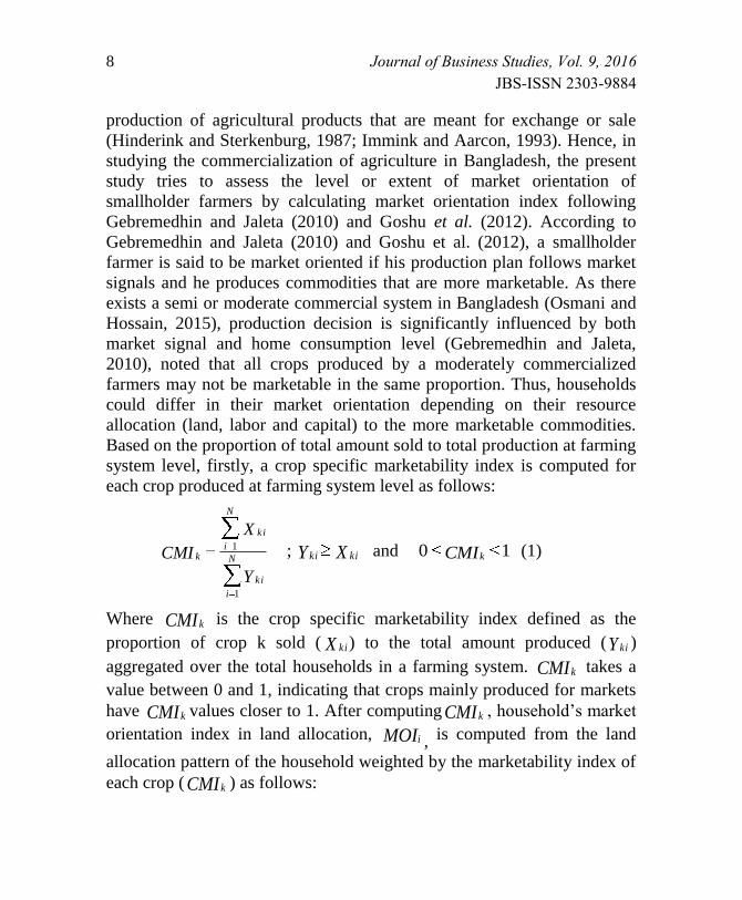
Based on the proportion of total amount sold to total production at farming
system level, firstly, a crop specific marketability index is computed for
each crop produced at farming system level as follows:
N
i
ki
N
i
ki
k
Y
X
CMI
1
1 ; XY kiki and 10 CMIk (1)
Where CMI k is the crop specific marketability index defined as the
proportion of crop k sold ( X ki) to the total amount produced (Y ki )
aggregated over the total households in a farming system. CMI k takes a
value between 0 and 1, indicating that crops mainly produced for markets
have CMI k values closer to 1. After computing CMI k , household‟s market
orientation index in land allocation, MOIi , is computed from the land
allocation pattern of the household weighted by the marketability index of
each crop ( CMI k ) as follows:
Journal of Business Studies, Vol. 9, 2016 9
JBS-ISSN 2303-9884
L
LCMI
MOI Ti
k
k
ikk
i1 ; L
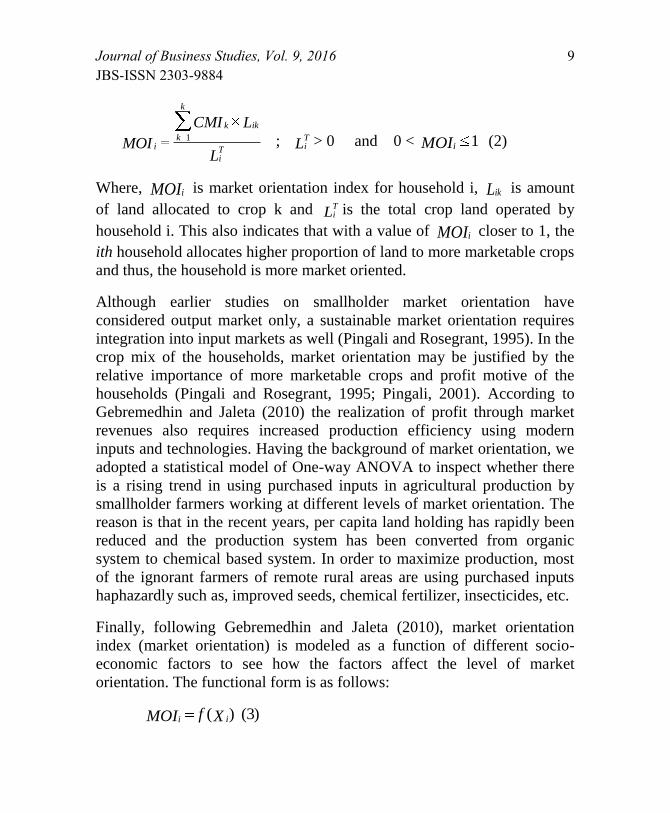
Ti > 0 and 0 < 1MOIi (2)
Where, MOIi is market orientation index for household i, Lik is amount
of land allocated to crop k and LTi is the total crop land operated by
household i. This also indicates that with a value of MOIi closer to 1, the
ith household allocates higher proportion of land to more marketable crops
and thus, the household is more market oriented.
Although earlier studies on smallholder market orientation have
considered output market only, a sustainable market orientation requires
integration into input markets as well (Pingali and Rosegrant, 1995). In the
crop mix of the households, market orientation may be justified by the
relative importance of more marketable crops and profit motive of the
households (Pingali and Rosegrant, 1995; Pingali, 2001). According to
Gebremedhin and Jaleta (2010) the realization of profit through market
revenues also requires increased production efficiency using modern
inputs and technologies. Having the background of market orientation, we
adopted a statistical model of One-way ANOVA to inspect whether there
is a rising trend in using purchased inputs in agricultural production by
smallholder farmers working at different levels of market orientation. The
reason is that in the recent years, per capita land holding has rapidly been
reduced and the production system has been converted from organic
system to chemical based system. In order to maximize production, most
of the ignorant farmers of remote rural areas are using purchased inputs
haphazardly such as, improved seeds, chemical fertilizer, insecticides, etc.
Finally, following Gebremedhin and Jaleta (2010), market orientation
index (market orientation) is modeled as a function of different socio-
economic factors to see how the factors affect the level of market
orientation. The functional form is as follows:
)3( )(XfMOI ii
10 Journal of Business Studies, Vol. 9, 2016
JBS-ISSN 2303-9884
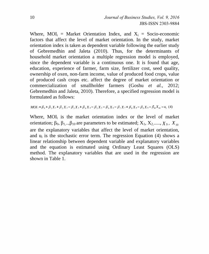
Where, MOIi = Market Orientation Index, and Xi = Socio-economic
factors that affect the level of market orientation. In the study, market
orientation index is taken as dependent variable following the earlier study
of Gebremedhin and Jaleta (2010). Thus, for the determinants of
household market orientation a multiple regression model is employed,
since the dependent variable is a continuous one. It is found that age,
education, experience of farmer, farm size, fertilizer cost, seed quality,
ownership of oxen, non-farm income, value of produced food crops, value
of produced cash crops etc. affect the degree of market orientation or
commercialization of smallholder farmers (Goshu et al., 2012;
Gebremedhin and Jaleta, 2010). Therefore, a specified regression model is
formulated as follows:
)4( 110109988776655443322110uXXXXXXXXXXMOI i
Where, MOIi is the market orientation index or the level of market
orientation; β0, β1,..,β10 are parameters to be estimated; X1, X2,....., X 9 , 10X
are the explanatory variables that affect the level of market orientation,
and ui is the stochastic error term. The regression Equation (4) shows a
linear relationship between dependent variable and explanatory variables
and the equation is estimated using Ordinary Least Squares (OLS)
method. The explanatory variables that are used in the regression are
shown in Table 1.
Journal of Business Studies, Vol. 9, 2016 11
JBS-ISSN 2303-9884
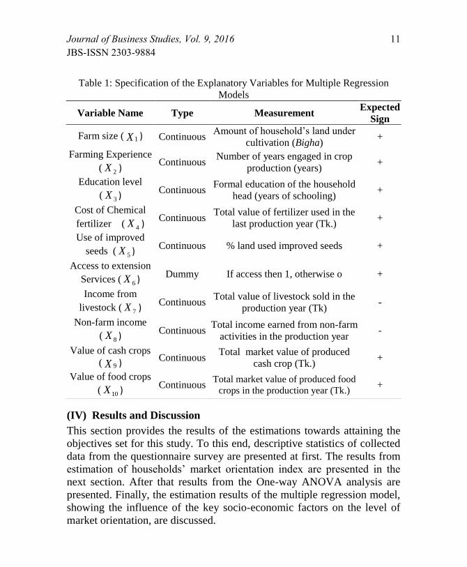
(IV) Results and Discussion
This section provides the results of the estimations towards attaining the
objectives set for this study. To this end, descriptive statistics of collected
data from the questionnaire survey are presented at first. The results from
estimation of households‟ market orientation index are presented in the
next section. After that results from the One-way ANOVA analysis are
presented. Finally, the estimation results of the multiple regression model,
showing the influence of the key socio-economic factors on the level of
market orientation, are discussed.
Table 1: Specification of the Explanatory Variables for Multiple Regression
Models
Variable Name Type Measurement Expected
Sign
Farm size ( X 1 ) Continuous Amount of household‟s land under
cultivation (Bigha) +
Farming Experience
( 2X ) Continuous
Number of years engaged in crop
production (years) +
Education level
( 3X ) Continuous
Formal education of the household
head (years of schooling) +
Cost of Chemical
fertilizer ( 4X ) Continuous
Total value of fertilizer used in the
last production year (Tk.) +
Use of improved
seeds ( 5X ) Continuous % land used improved seeds +
Access to extension
Services ( 6X ) Dummy If access then 1, otherwise o +
Income from
livestock ( 7X ) Continuous
Total value of livestock sold in the
production year (Tk) -
Non-farm income
( 8X ) Continuous
Total income earned from non-farm
activities in the production year -
Value of cash crops
( X 9 ) Continuous Total market value of produced
cash crop (Tk.) +
Value of food crops
( 10X ) Continuous
Total market value of produced food
crops in the production year (Tk.) +

12 Journal of Business Studies, Vol. 9, 2016
JBS-ISSN 2303-9884
Descriptive Statistics
Analyses of the demographic and socio-economic characteristics revealed that substantial difference exists among the sample smallholder farmers of the study area. Although farm size, farming experience, education level, cost of chemical fertilizer, use of improved seeds, access to extension services, income from livestock, non-farm income, value of cash crops and value of food crops were hypothesized to be the common factors affecting commercialization, significant variations across farmers with respect to information of these variables were found. Moreover, to check whether all variables used in this study really tap into one construct from the questionnaire, we used Cronbach‟s Alpha Test of Reliability. It is an important concept in the evaluation of assessments and questionnaires which measures the internal consistency or reliability of the variables (Tavakol and Dennick, 2011). The coefficient Alpha (α) in this test ranges from 0 to 1, that is, if all variables are perfectly reliable and measure the same thing (true score), then α is equal to 1 and if there is no true score but only error in the items, then α is equal to 0. In this study, the coefficient Alpha (α) is found as 0.781 which is considered “good level of reliability” as far as social science research is concerned (Cronbach, 1951; Nunnally & Bernstien, 1994). The descriptive statistics of the variables used in the present study are shown in Table 2.
Table 2: Socio-economic Characteristics of Smallholder Farmers
Variables Mean Std. Dev. Min. Max.
Farm size (bigha) 4.01 1.824892 0.65 7
Farming Experience (years) 25.68 11.62623 4 45
Education level (years of schooling) 5.4 5.270463 0 20
Cost of Chemical fertilizer (Tk.) 6467.41 3256.146 1578 17180
Use of improved seeds (% of
cultivated land) 84.48 31.12005 0 100
Income from livestock (Tk.) 20204 25788.87 0 110000
Non-farm income (Tk.) 37252 61529.35 0 400000
Value of cash crops (Tk.) 46126.5 56299.27 0 284000
Value of food crops (Tk.) 57983.3 44550.57 5600 252000
Note: Tk. indicates Bangladeshi currency, taka
Source: Authors‟ calculations according to data from Osmani and Hossain (2013)
Journal of Business Studies, Vol. 9, 2016 13
JBS-ISSN 2303-9884
From the table it is found that the average farm size of a sample farmer is
4.01 bigha indicating that most of the farmers in the study area are
smallholders. It is also found that all farmers in the study area do not have
same experience. Table 2 shows that the average experience of the sample
farmers is 25.68 years, where minimum experience is 4 years and
maximum experience is 45 years. The average level of education of
farmers in the study area is 5.4 years of schooling with minimum of no
education and maximum of 20 years of schooling. Chemical fertilizer is an
important input for agricultural production in the study area. The average
cost of chemical fertilizer of the sample farmers is Tk.6467.41 in a crop
year. From the above table, it is observed that in 2013-14 production
season, about 84.48% of cultivated land of the sample farmers was under
the use of improved seeds. It is also seen that average annual income from
livestock asset is Tk.20244, whereas average annual non-farm income is
Tk. 37252. Farmers in the study area produce mainly food and cash crops.
It is found that the average value of produced food crops of the sample
farmers is Tk.57983.3 and that of cash crop is Tk.46126.5.
Level of Market Orientation of Smallholder Farmers
In explaining the level of market orientation of smallholder farmers in
Durgapur Upazila, we adopted a household market orientation index. As
indicated earlier, households‟ commercialization behavior can be reflected
by their land allocation pattern and the crop marketability index is used as
an indicator of the households‟ market orientation. The market orientation
index is computed for specific crops produced in 2013 production season.
The findings of market orientation index reflect that the land allocation
decision of households is designed for profit maximization. Specifically,
on average, smallholder farmers in the study area allocate 59% of their
cultivable land to the production of marketable crops and as the average
market orientation index is about 0.59, indicating a moderate market
orientation of smallholder farmers in the study area (Table 3). The
computed results from crop marketability index and household market
orientation index are presented in Table 3.
14 Journal of Business Studies, Vol. 9, 2016
JBS-ISSN 2303-9884
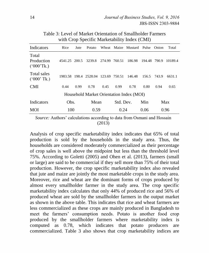
Table 3: Level of Market Orientation of Smallholder Farmers
with Crop Specific Marketability Index (CMI)
Indicators Rice Jute Potato Wheat Maize Mustard Pulse Onion Total
Total
Production
(„000‟Tk.)
4541.25 200.5 3239.8 274.99 760.51 186.98 194.48 790.9 10189.4
Total sales
(„000‟ Tk.) 1983.58 198.4 2528.04 123.69 750.51 146.48 156.5 743.9 6631.1
CMI 0.44 0.99 0.78 0.45 0.99 0.78 0.80 0.94 0.65
Household Market Orientation Index (MOI)
Indicators Obs. Mean Std. Dev. Min Max
MOI 100 0.59 0.24 0.06 0.96
Source: Authors‟ calculations according to data from Osmani and Hossain
(2013)
Analysis of crop specific marketability index indicates that 65% of total
production is sold by the households in the study area. Thus, the
households are considered moderately commercialized as their percentage
of crop sales is well above the midpoint but less than the threshold level
75%. According to Goletti (2005) and Ohen et al. (2013), farmers (small
or large) are said to be commercial if they sell more than 75% of their total
production. However, the crop specific marketability index also revealed
that jute and maize are jointly the most marketable crops in the study area.
Moreover, rice and wheat are the dominant forms of crops produced by
almost every smallholder farmer in the study area. The crop specific
marketability index calculates that only 44% of produced rice and 56% of
produced wheat are sold by the smallholder farmers in the output market
as shown in the above table. This indicates that rice and wheat farmers are
less commercialized as these crops are mainly produced in Bangladesh to
meet the farmers‟ consumption needs. Potato is another food crop
produced by the smallholder farmers where marketability index is
computed as 0.78, which indicates that potato producers are
commercialized. Table 3 also shows that crop marketability indices are
Journal of Business Studies, Vol. 9, 2016 15
JBS-ISSN 2303-9884
0.78, 0.80 and 0.94 for mustard, pulse and onion, respectively, although
farmers are less interested in production of these types.
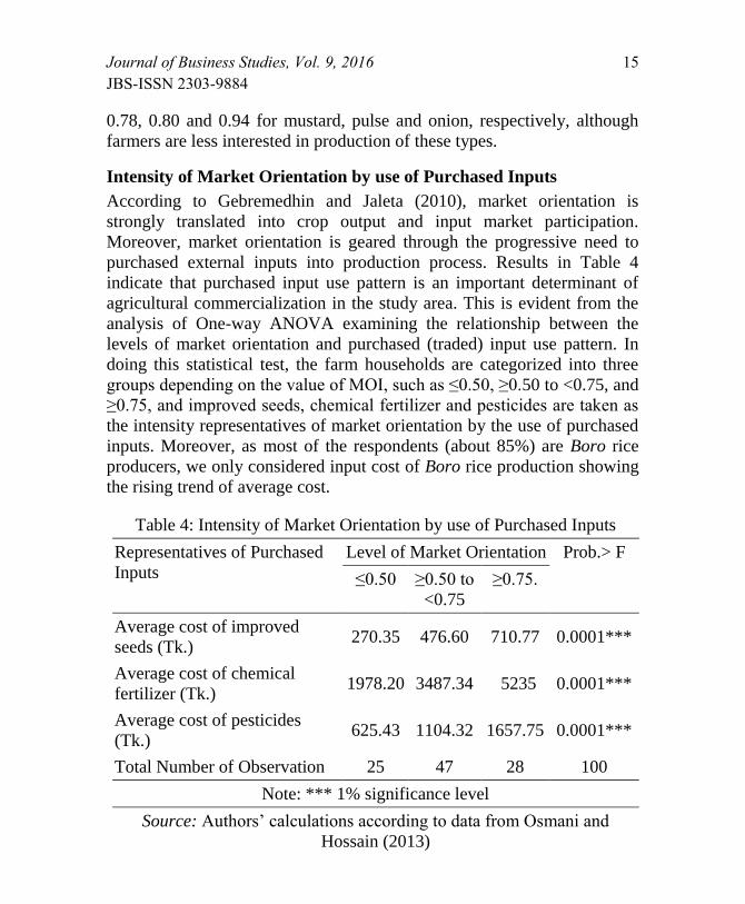
Intensity of Market Orientation by use of Purchased Inputs
According to Gebremedhin and Jaleta (2010), market orientation is
strongly translated into crop output and input market participation.
Moreover, market orientation is geared through the progressive need to
purchased external inputs into production process. Results in Table 4
indicate that purchased input use pattern is an important determinant of
agricultural commercialization in the study area. This is evident from the
analysis of One-way ANOVA examining the relationship between the
levels of market orientation and purchased (traded) input use pattern. In
doing this statistical test, the farm households are categorized into three
groups depending on the value of MOI, such as ≤0.50, ≥0.50 to <0.75, and
≥0.75, and improved seeds, chemical fertilizer and pesticides are taken as
the intensity representatives of market orientation by the use of purchased
inputs. Moreover, as most of the respondents (about 85%) are Boro rice
producers, we only considered input cost of Boro rice production showing
the rising trend of average cost.
Table 4: Intensity of Market Orientation by use of Purchased Inputs
Representatives of Purchased
Inputs
Level of Market Orientation Prob.> F
≤0.50 ≥0.50 to
<0.75
≥0.75.
Average cost of improved
seeds (Tk.) 270.35 476.60 710.77 0.0001***
Average cost of chemical
fertilizer (Tk.) 1978.20 3487.34 5235 0.0001***
Average cost of pesticides
(Tk.) 625.43 1104.32 1657.75 0.0001***
Total Number of Observation 25 47 28 100
Note: *** 1% significance level
Source: Authors‟ calculations according to data from Osmani and
Hossain (2013)
16 Journal of Business Studies, Vol. 9, 2016
JBS-ISSN 2303-9884
Table 4 shows the intensity of market orientation of smallholder farmers
by the use of purchased inputs in the production of agricultural
commodities. The results presented in the table showed that the use of
purchased inputs has consistent increasing pattern along the level of
market orientation, from low to high. The One-way ANOVA test results
confirm that the variation in average costs of improved seeds, chemical
fertilizer and pesticides by farm households at different levels of market
orientation is statistically significant at 1% significance level.
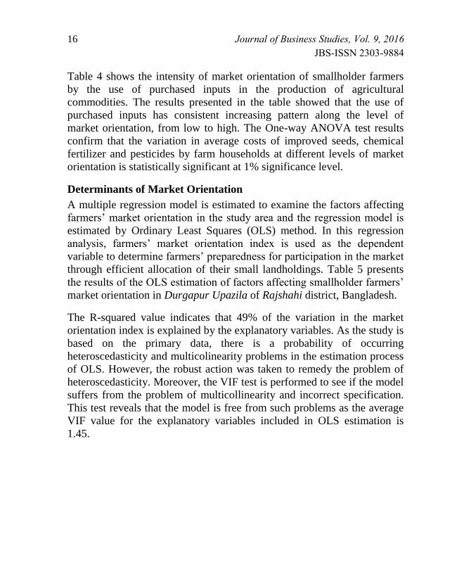
Determinants of Market Orientation
A multiple regression model is estimated to examine the factors affecting
farmers‟ market orientation in the study area and the regression model is
estimated by Ordinary Least Squares (OLS) method. In this regression
analysis, farmers‟ market orientation index is used as the dependent
variable to determine farmers‟ preparedness for participation in the market
through efficient allocation of their small landholdings. Table 5 presents
the results of the OLS estimation of factors affecting smallholder farmers‟
market orientation in Durgapur Upazila of Rajshahi district, Bangladesh.
The R-squared value indicates that 49% of the variation in the market
orientation index is explained by the explanatory variables. As the study is
based on the primary data, there is a probability of occurring
heteroscedasticity and multicolinearity problems in the estimation process
of OLS. However, the robust action was taken to remedy the problem of
heteroscedasticity. Moreover, the VIF test is performed to see if the model
suffers from the problem of multicollinearity and incorrect specification.
This test reveals that the model is free from such problems as the average
VIF value for the explanatory variables included in OLS estimation is
1.45.
Journal of Business Studies, Vol. 9, 2016 17
JBS-ISSN 2303-9884
Table 5: OLS Estimation Results for Determinants of Market Orientation
Variable Coefficient Robust
Std. Err. T P>|t|
Farm size ( X 1 ) 0.028** 0.013 2.09 0.040
Farming Experience ( 2X ) 0.002 0.002 1.23 0.221
Education level ( 3X ) 0.002 0.004 0.52 0.605
Cost of Chemical fertilizer
( 4X ) 3.45e-06 6.46e-06 0.53 0.595
Use of improved seeds
( 5X ) 0.002*** 0.001 2.86 0.005
Access to extension Services
( 6X ) 0.099** 0.047 2.11 0.038
Income from livestock ( 7X ) -6.38e-08 7.43e-07 -0.09 0.932
Non-farm income ( 8X ) -3.50e-07 3.44e-07 -1.02 0.312
Value of cash crops ( X 9 ) 1.30e-
04*** 3.37e-07 3.86 0.000
Value of food crops ( 10X ) 1.93e-07 4.76e-07 0.41 0.686
Constant 0.146 0.079 1.84 0.069
F( 10, 89) = 11.92; Prob. > F = 0.0000; R-squared =0.4867; Root MSE
=0.17835
Note: *** and ** indicate 1% and 5% significance levels, respectively
Source: Authors‟ calculations according to data from Osmani and
Hossain (2013)
Table 5 shows the results from the OLS estimation of the determinants of
market orientation of smallholder farmers. The result indicates that that
the extent of market orientation by smallholder farmers is significantly
determined by farm size, use of improved seeds, access to extension
services and value of produced cash crops. That is, these variables have
stronger numerical effects on market orientation. Other explanatory
variables have no significant impact on market orientation of the small
holder farmers. It is found that there is a strong significant and positive
relationship between farm size and market orientation in the study area i.e.
(β = 0.028; P = 0.040). This indicates that if farmers‟ farm size is
18 Journal of Business Studies, Vol. 9, 2016
JBS-ISSN 2303-9884
increased by one bigha, market orientation index will be increased by
0.028 at 5% significance level. The fact might be that farm households
with large farm size could allocate their land for cash crop production
giving them better position to participate in the output market. The
regression result also revealed that use of improved seeds has a significant
and positive impact (β = 0.002; P = 0.005) on the market orientation
index. It explains that at 1% significance level, farm households‟ market
orientation increases by 0.20% if they use 1% more land for cultivation by
using improved seeds. This is so because use of improved seeds renders
higher production and improved seeds are supposed to be effective to
produce high quality crops resulting from high demand and possible
higher selling price for the crop.
Agricultural extension services appeared effective in inducing market
orientation for Bangladeshi smallholder farmers. The result of table 5
shows that farmers‟ access to extension services are (β = 0.0993; P =
0.038) related significantly and positively with the market orientation in
the study area. This explains that if agricultural extension services are
locally available to the smallholder farmers then their market orientation is
expected to rise by 0.099. The result may be attributed to the effective
monitoring and teaching approach of the extension agents and expert
persons in the study area. Finally, the amount of total cash crop production
(β = 1.30e-06; P = 0.000) is also strongly and positively related with
market orientation of smallholder farmers in the study area. This explains
that as value of cash crop production increases by 1 Tk., the extent of
market orientation increases by 0.00013.
(V) Conclusion
Commercialization is a new paradigm in Bangladesh agriculture.
Generally, Bangladeshi smallholder farmers have integrated into the
market system with their surplus production. This also leads to progressive
substitution of non-traded inputs in favor of purchased inputs in crop
production. Thus, this study puts emphasis on the analysis of the
potentiality of Bangladeshi smallholder farmers in enhancing farmers‟
involvement in commercial agriculture. The calculation of household
market orientation index reveals that on the average, farm households
allocate 59% of their cultivable land to the production of marketed crops.

Journal of Business Studies, Vol. 9, 2016 19
JBS-ISSN 2303-9884
This is because of the gradual substitution of complex farming system in
the study area by specialized farmers for specific high value crops in
which every farm decision depends on the market signals. It is also
important to note that as farmers in the study area are moderately market
orientated, they progressively use traded inputs like improved seeds,
chemical fertilizer and pesticides in production. One-way ANOVA test
finds that farm households are overwhelmingly using purchased inputs in
production as they move from lower to higher level of market orientation.
However, one of the key limiting factors in production is that although
farmers are somewhat market oriented, the production system is not yet
fully mechanized. Moreover, ownership or availability of factors is not
likely to be complementary to external inputs for the smallholder farmers
in the study area. Thus, for proper interventions to promote input market
orientation in terms of using more land for cultivation by using traded
inputs may need to address the problem of availability of complementary
inputs.
Moreover, the result of OLS estimation shows that market orientation of
smallholder farmers increases as the farmers with relatively larger farm
size are using more improved seeds and have well accessed to extension
services for production of cash crops. Specifically, these findings suggest
that a holistic approaches should be taken that would enforce farmer-
market contracts and fair input prices, adequate extension services for all
marginal and smallholder farmers and encourage farmers to produce and
trade market oriented crops, such as onion, pulse, maize, jute and potato.
Along these lines, there is a need to promote market oriented crop
technologies and further research on endogenous determinants of market
orientation also deserves better attention.
20 Journal of Business Studies, Vol. 9, 2016
JBS-ISSN 2303-9884
References
Adenegan, K.O., Olorunsomo, S.O. and Nwauwa, L.O.E., (2013),
“Determinants of Market Orientation among Smallholders Cassava
Farmers in Nigeria”, Global Journal of Management and Business
Research Finance, Volume 13, Issue 6, Version 1.0.
Atuahene-Gima, K., (1995), “An exploratory analysis of the impact of
market orientation on new product performance: A contingency
approach”, J. Prod. Innovat. Manag., 12: 275-293.
Azad, S.A.K., (2015), “High-Value Agriculture Products in Bangladesh:
An Empirical Study on Agro-Business Opportunities and
Constraints”, Dhaka University Institutional Repository, A Ph. D.
Thesis submitted to the Department of Marketing, University of
Dhaka.
BBS, (2013), “Macroeconomic indicators”, Bangladesh Bureau of
Statistics, Ministry of Finance, Government of the People‟s
Republic of Bangladesh.
BBS, (2011), “Bangladesh Population Census”, Bangladesh Bureau of
Statistics, Ministry of Finance, Government of the People‟s
Republic of Bangladesh.
Balint, B.E., (2003), “Determinants of Commercial Orientation and
Sustainability of Agricultural Production of the Individual Farms
in Romania”, PhD Dissertation, University of Bonn, Germany.
Chamberlin, J., (2008), “It‟s a Small World After All, Defining
Smallholder Agriculture in Ghana”, paper presented at
International Food Policy Research Institute (IFPRI), IFPRI
Discussion Paper 00823.
Cronbach, L.F., (1951), “Coefficient alpha and the internal structure of
tests”, Psychometricka, 16, 297-334.
De Janvry, A., Fafchamps, M. and Sadoulet. E. (1991), “Peasant
Household Behavior with Missing Markets: Some Paradoxes
Explained,” The Economic Journal, 101(409):1400-1417.

Journal of Business Studies, Vol. 9, 2016 21
JBS-ISSN 2303-9884
Davis, J.R., (2006), “How can the poor benefit from the growing markets
for high value agricultural products?”, Research Report, Natural
Resources Institute, Kent, UK.
Dixon, J., Taniguchi, K. and Wattenbach, H., Eds., (2003), “Approaches
to assessing the impact of globalization on African smallholders:
Household and village economy modeling”, Proceedings of a
working session on Globalization and the African Smallholder
Study, Food and Agriculture Organization of the United Nations.
Fritz, W., (1996), “Market Orientation and Corporate Success: Findings
from Germany”, European Journal of Marketing, Vol 30(8): 59-
74.
Gabre-Madhin, E.Z., and Haggblade, S., (2004), “Successes in African
Agriculture: Results of an Expert Survey.” World Development 32
(5): 745–766.
Gebremedhin, B. and Jaleta, M., (2010), “Commercialization of
Smallholders: Is Market Participation Enough?” Joint 3rd
African
Association of Agricultural Economists (AAAE) and 48th
Agricultural Economists Association of South Africa (AEASA)
Conference, Cape Town, South Africa.
Gebremedhin, B. and Jaleta, M., (2012), “Market orientation and market
participation of smallholders in Ethiopia: Implications for
commercial transformation”, Proceeding of International
Association of Agricultural Economists (IAAE) Triennial
Conference. Foz do lguacu, Brazil.
Goletti, F., (2005), “Agricultural Commercialization, Value Chains and
Poverty Reduction, Making Markets World Better for the
Poor”, Discussion Paper no.7, Hanoi: Asian Development
Bank.
Goshu, D., Kassa, B. and Ketema, M., (2012), “Measuring Smallholder
Commercialization Decision and Interaction in Ethiopia”, Journal
of Economics and Sustainable Development. ISSN 2222-1700
(Paper) ISSN 2222-2855 (Online), Vol.3, No.13.
22 Journal of Business Studies, Vol. 9, 2016
JBS-ISSN 2303-9884
GoB (Government of Bangladesh), (2008). Handbook of Agricultural
Statistics, December 2007, Ministry of Agriculture, Government of
the People‟s Republic of Bangladesh, Dhaka.
Greenley, G.E., (1995), “Market orientation and company performance:
Empirical evidence from UK companies”, Brit. J. Manage., 6: 1-13.
Haggblade, S., & Hazell, P.B.R., (2010), “Successes in African
Agriculture: Lessons for the Future”, Baltimore: Johns Hopkins
University Press.
Hazell, P., Poulton, C., Wiggins, S. and Dorward, A., (2007), “The Future
of Small Farms for Poverty Reduction and Growth”, 2020
Discussion Paper No. 42. IFPRI, Washington, D.C.
Harris, L.C. and Piercy, N.F., (1999), “Management behavior and barriers
to market orientation in retailing companies”, Journal of Services
Marketing, 13(2): 113-131.
Helfert, G., Ritter, T. and Walter, A., (2001), “How does market
orientation affect business relationships?”, Proceeding of the 17th
IMP Conference, Oslo, September 9-11, pp: 1-26.
Hinderink, J. and Sterkenbur, J.J., (1987), “Agricultural
Commercialization and Government Policy in Africa”, KPI
Limited, New York.
Immink, M.D.C and Alarcon, J.A., (1993), “Household Income, Food
Availability, and Commercial Crop Production by Smallholders
Farmers in the Western Hifghlands of Guatemala”, Economic
Development and Cultural Change, 41: 319-342
IFPRI (International Food Policy Research Institute), (2005), “The future
of small farms: Proceedings of a research workshop”, Wye, UK,
June 26-29, Washington, DC.
Jaleta, M., Gebremedhin, B. and Hoekstra, D., (2009), “Smallholder
commercialization: Processes, determinants and impact. ILRI
Discussion Papers, No. 18. Improving Productivity and Market
Success (IPMS) of Ethiopian Farmers Project. International
Livestock Research Institute (ILRI), Nairobi, Kenya.
Journal of Business Studies, Vol. 9, 2016 23
JBS-ISSN 2303-9884
Jayne, T.S., Mukumbu, M., Duncan, J., Lundberg, M., Aldridge, Staatz, J.,
Howard, J.K., Nakaponda, B., Ferris, J., Keita, F. and
Sananankoua, A.K., (1995), “Trends in real food prices in six Sub-
Sahara African countries”, Policy synthesis Number 2 East
Lansing: Michigan State University.
Johnston, B.F., & Mellor, J.W., (1961), “The Role of Agriculture in
Economic Development”, American Economic Review 51 (4):
566–593.
Johnston, B.F., (1970), “Agriculture and Structural Transformation in
Developing Countries: A Survey of Research”, Journal of
Economic Literature 8 (2): 369–404.
Jaworski, B.J. and Kohli, A.K., (1993), “Market Orientation: antecedents
and consequences”, Journal of Marketing, Vol. 57(3): 53-70.
Leavy, J. and Poulton, C., (2007), “Commercializations in Agriculture”,
Future Agricultures Consortium, working paper 003.
Mahelet, G.F (2007), Factors Affecting Commercialization of Smallholder
Farmers in Ethiopia, Ministry of Finance and Economic
Development (MoFED) GTP, Volume I: Maintext (2010).
Narver, J.C. and Slater, S.F., (1990), “The effect of marketing orientation
on business profitability”, Journal of Marketing, Vol. 4(1): 20-36.
Nagayets, O., (2005), “Small Farms: Current Status and Key Trends”,
Information Brief Prepared for the Future of Small Farms Research
Workshop, Wye College.
Narayanan, S., and Gulati. A., (2002), “Globalization and the
smallholders: A review of issues, approaches, and implications.
Markets and Structural Studies Division”, International Food
Policy Research Institute, Discussion Paper No. 50. Washington,
D.C.
Nunnally, J.C. and Bernstien, I.H., (1994), “Psychometric theory 3”, New
York: McGraw-Hill.
24 Journal of Business Studies, Vol. 9, 2016
JBS-ISSN 2303-9884
Ohen, S.B., Etuk, E.A., Onoja, J.A., (2013), “Analysis of Market
Participation by Rice Farmers in Southern Nigeria”, Journal of
Economics and Sustainable Development, vol. 4, no. 7, pp. 6-11.
Osmani, M.A.G. and Hossain, E., (2013), “Household survey-2013:
Commercialization of smallholder farmers and its welfare
outcome”, Department of Economics, University of Rajshahi,
Rajshahi-6205, Bangladesh.
Osmani, M.A.G., Islam, M.K., Ghosh, B.C. and Hossain, M.E., (2014),
“Commercialization of Smallholder Farmers and Its Welfare
Outcomes: Evidence from Durgapur Upazila of Rajshahi District,
Bangladesh” Journal of World Economic Research, Vol. 3, No. 6,
2014, pp. 119-126.
Osmani, M.A.G. and Hossain, E., (2015), “Market Participation Decision
of Smallholder Farmers and its Determinants in Bangladesh”,
Economics of Agriculture, Vol. (62), No. 1 (163-179).
Pingali, P.L. and Rosegrant, M.W., (1995), “Agricultural
commercialization and diversification: Process and polices”, Food
Policy, 20(3):171-185.
Pingali, P.L., (1997), “From Subsistence to Commercial Production
Systems: The Transformation of Asian Agriculture”, American
Journal of Agricultural Economics, 79(2): 628-634.
Pingali, P.L., (2001), “Environmental consequences of agricultural
commercialization in Asia” Environment and Development
Economics, null, pp 483-502.
Pingali, P., Khwaja, Y. and Meijer, M., (2005), “Commercializing small
farmers: Reducing transaction costs”, FAO/ESA Working Paper
No. 05-08. Food and Agriculture Organization of the United
Nations, Rome, Italy.
Pingali, P.L., (2010), “Agriculture Renaissance: Making “Agriculture for
Development” Work in the 21st Century”, Handbook Agric. Econ.
4:3867-3894. Elsevier.
Journal of Business Studies, Vol. 9, 2016 25
JBS-ISSN 2303-9884
Razzaque, M.A., Hossain, M.G., (2007), “Country Report on the State of
Plant Genetic Resources for Food and Agriculture”, Ministry of
Agriculture Bangladesh.
Sharma, V.P., Jain, D. and Sourovi, D., (2012), “Managing agricultural
commercialization for inclusive growth in South Asia”, Agriculture
Policy Series, Briefing Paper No. 6/2012, GDN, New Delhi, India.
Selnes, F., Jaworski, B.J. and Kohli, A.K., (1996), “Market Orientation in
United States and Scandinavian Companies: A cross-cultural
study”, Scandinavian Journal of Management, Vol 12(2): 139-157.
SFB (Syngenta Foundation Bangladesh), (2015), “Improving the
Livelihood of Smallholder Farmers”, available at:
www.syngentafoundation.org/index.cfm?pageID=579.
Thapliya, J.N., (2006), “Constraints and Approaches for Developing
Market Access and Vertical Linkages in High Value Agriculture”,
A Policy Paper (16) prepared for Economic Policy Network and
Asian Development Bank, Confederation of Nepalese Industries
(CNI) 303 Bagmati Chambers, Teku, Kathmandu, Nerpal.
Timmer, C.P., (1997), “Farmers and Markets: The Political Economy of
New Paradigms”, American Journal of Agricultural Economics,
79(2): 621-627.
Tavakol, M. and Dennick, R., (2011), “Making sense of Cronbach‟s
alpha”, International Journal of Medical Education, Vol. 2:53-55.
von Braun, J. and Kennedy, E. (Eds.), (1994), “Agricultural
Commercialization, Economic Development, and Nutrition”, Johns
Hopkins University Press, Baltimore.
von Braun, J., (1995), “Agricultural commercialization: impacts on
income and nutrition and implications for policy”, Food Policy, 20
(3): 187 – 202.
Wegner, L. and Zwart, G., (2011), “Who will Feed the World? The
Production Challenge”, Oxfam Research Report, www.oxfam.org.
World Bank, (2013), “World Development Indicators: Rural environment
and land use”, World Bank, Washington, DC.
Journal of Business Studies, Vol. 9, 2016 26
JBS-ISSN 2303-9884
Factors Affecting the Choices for Off-farm Activities in
Bangladesh: A Study of Rajshahi District
Dr. A S M Kamruzzaman
Abstract
People living in rural and semi-urban areas in Bangladesh are taking
heterogeneous income generating off-farm activities to reduce poverty. But the
participation in any employment activity or sector depends on both motivational
and ability factors. The capacity of individuals or households to participate in
such activities is not uniform. Poverty, inequality and human skills affect the
capacity of individuals or households to engage in their preferred high
remunerative off-farm activities. This paper has identified some demographic and
socio-economic ability factors of rural individuals and households to engage in
some selected off-farm activities in the study area. These factors were found to
have affected significantly the decisions of households to choose or participate in
some sample off-farm activities. Age of entrepreneur, family size, whether the
head of the family or not, education, training, past experience, social network,
loan diversion for other purposes, household land ownership, percentage of off-
farm income in total household income, percentage of equity and debt fund
invested in business, distance between the local bank branch and the residence of
an entrepreneur, and distance between the local market and the residence of an
entrepreneur were found as significant factors to affect the choices for a
particular off-farm activity in the study. The multinomial logistic regression
analysis was used for modeling the choices of off-farm activities. A randomly
selected, cross-sectional, sample survey data of 300 borrowers from the SECP
program of RAKUB, purposively selected under five categories of sample off-
farm activities, had been used in this study.
Keywords: Rural livelihood diversification, ability factors of rural entrepreneurs,
natural, human, social and financial capital
(I) Introduction
ural and semi-urban people are taking heterogeneous income
generating activities besides their main occupations to reduce the
Associate Professor, Department of Finance, University of Rajshahi
Email : [email protected]
R

Journal of Business Studies, Vol. 9, 2016 27
JBS-ISSN 2303-9884
overall risk of livelihood, or to take opportunities for higher remunerative
jobs than less remunerative traditional agriculture (Davis and Bezemer
2004). In developing countries, the resource-poor farmers are usually risk-
averse and, therefore, they will allocate less time to more risky jobs or,
alternatively, they will be willing to accept lower wages in the less-risky
environment. Rural farmers may participate in off-farm activities only to
reduce the overall risk of their incomes or to increase their total returns
(NRI, 2000)1.
Participation in any employment sector depends on both motivational and
ability factors. The first is the incentive or motivation – perhaps higher
return or less risk than alternatives. The second is the capacity of an
individual or household– perhaps certain skills or making necessary
financial commitment. It is often the poorest households who have the
highest motivation to diversify their livelihoods and also have the highest
constraints to diversify. Poverty, inequality in income and wealth, and
human skills affect the ability of an individual or household to engage in
the preferred activity or sector.
Although the choice and the participation in any rural off-farm activity for
self-employment depend on the motivation and the ability factors, the
capacity of households or individuals is not uniform. The analysis of 100
farm-households (Reardon et al 2000) shows a rough pattern of the
capacity of rural households : a positive relationship between non-farm
income share (and level) and total household income or Land-holding in
much of Africa; a negative relationship in much of Latin America, and a
very mixed set of results in Asia. They argue that the positive relationship
and the U-curve relationship (mixed results) reflect high entry barriers for
poor households to engage in nonfarm self-employment activities in
Africa and Asia.
Factors determining access to high remunerative nonfarm jobs can be of
individual, household, region or place, and project specific. Ellis and
Hussein (1998) in their study identified health and nutrition, household
1 Policy and Research on the Rural Non-Farm Economy: A Review of Conceptual, Methodological
and Practical Issues, Draft paper, NRI RNFE Project Team, November 2000.
28 Journal of Business Studies, Vol. 9, 2016
JBS-ISSN 2303-9884
composition, access to finance, education, social capital and infrastructure
as determining factors to have access in nonfarm jobs. These factors are
considered as assets, or factors of production, or capital representing the
capacity of household to diversify income or livelihood. In some
livelihood literature (i.e. Barrett and Reardon 2000; Ellis 2000; and
Carney 1998) factors affecting the choice, or the access of households
were classified as: natural capital (access to land or common property
resources); social capital (networks and organizations); human capital
(health and educational status); financial capital; and physical capital (hard
infrastructure, shelter and production equipments).
As population pressure increases and rapid unplanned urbanization takes
place, it has become more difficult for the rural poor to rely only on
agriculture or natural-resource-based activities. Even for many,
livelihoods have become less secure and sources of incomes have more
varied. The alternative to reduce overall risk of livelihoods or to diversity
incomes, and to take opportunities to relatively high remunerative jobs
will require some ability factors of individuals or households suitable to
have better access in it. Therefore, it is important to understand who have
access to alternative or supplementary activities that can bring sustained
and significant improvements in incomes or welfare for the individuals or
households concerned. A clear understanding of the entry-barriers faced
by different groups within the society, or even individuals within a
household is, therefore, very useful and important to academics,
institutions providing micro or SME finance, and particularly for policy
makers. Specially, financial institutions which are providing micro or
SME finance in different activity-based projects to alleviate poverty or to
develop entrepreneurial base for SME, may be benefited from this study
being better informed about the groups of entrepreneurs suitable for
heterogeneous off-farm activities.
(II) Objective of the study
This study attempts to identify the ability factors of rural households that
affect their choices for heterogeneous off-farm activities to diversify
incomes. The study has explored the capacity of individuals or households
to engage in off-farm activities crossing varying levels of entry barriers
with various forms capital (human, financial, social etc). Therefore, the
Journal of Business Studies, Vol. 9, 2016 29
JBS-ISSN 2303-9884
study has segregated the socio-economic, demographic and other factors
of rural households that determine the access to the preferred high
remunerative off-farm activities.
(III) Methods of Analysis
Logistic regression method has been used for modeling the choices of
households for some selected sample off-farm activities. Since the forms
of choices or the categories of the dependent variable are more than two or
multi-categorical, the multinomial logistic regression analysis is used to
predict the probability of being in the specific sample category of the
dependent variable for a set of independent variables or factors. A
sequential description on the estimation model, data and variables are
presented below in this section:
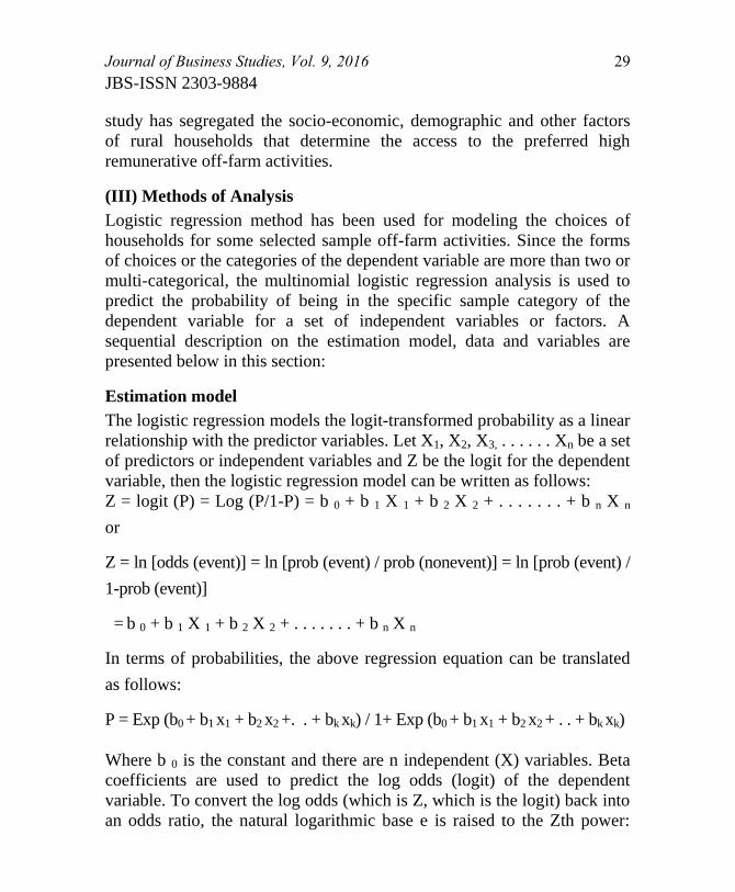
Estimation model
The logistic regression models the logit-transformed probability as a linear
relationship with the predictor variables. Let X1, X2, X3, . . . . . . Xn be a set
of predictors or independent variables and Z be the logit for the dependent
variable, then the logistic regression model can be written as follows:
Z = logit (P) = Log (P/1-P) = b 0 + b 1 X 1 + b 2 X 2 + . . . . . . . + b n X n
or
Z = ln [odds (event)] = ln [prob (event) / prob (nonevent)] = ln [prob (event) /
1-prob (event)]
= b 0 + b 1 X 1 + b 2 X 2 + . . . . . . . + b n X n
In terms of probabilities, the above regression equation can be translated
as follows:
P = Exp (b0 + b1 x1 + b2 x2 +. . + bk xk) / 1+ Exp (b0 + b1 x1 + b2 x2 + . . + bk xk)
Where b 0 is the constant and there are n independent (X) variables. Beta
coefficients are used to predict the log odds (logit) of the dependent
variable. To convert the log odds (which is Z, which is the logit) back into
an odds ratio, the natural logarithmic base e is raised to the Zth power:
30 Journal of Business Studies, Vol. 9, 2016
JBS-ISSN 2303-9884
odds (event) = exp (Z). Exp (Z) is the log odds of the dependent, or the
estimate of the odds of event.
Logistic regression estimates parameter values for b0, b1, b2 …..bn through
the Maximum Likelihood Estimation (MLE).
Data, Sample and Statistical tool
A cross-sectional sample survey data of 300 borrowers from the SECP
program of RAKUB, randomly collected from eleven than areas of
Rajshahi district, under purposively selected five categories of sample off-
farm activities popular in the sample area has been used in the analysis.
The SPSS package (11.5 Version) was used to analyze the data. The
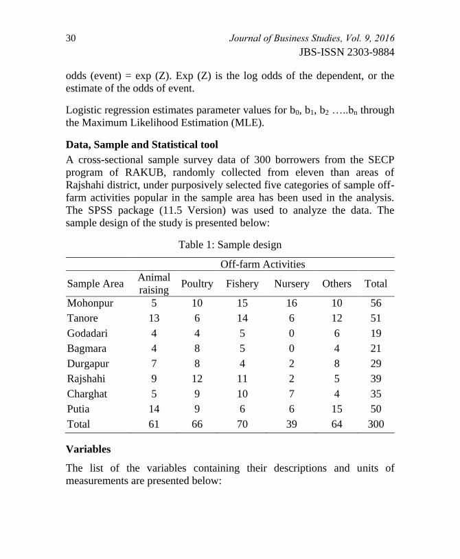
sample design of the study is presented below:
Table 1: Sample design
Off-farm Activities
Sample Area Animal
raising Poultry Fishery Nursery Others Total
Mohonpur 5 10 15 16 10 56
Tanore 13 6 14 6 12 51
Godadari 4 4 5 0 6 19
Bagmara 4 8 5 0 4 21
Durgapur 7 8 4 2 8 29
Rajshahi 9 12 11 2 5 39
Charghat 5 9 10 7 4 35
Putia 14 9 6 6 15 50
Total 61 66 70 39 64 300
Variables
The list of the variables containing their descriptions and units of
measurements are presented below:
Journal of Business Studies, Vol. 9, 2016 31
JBS-ISSN 2303-9884
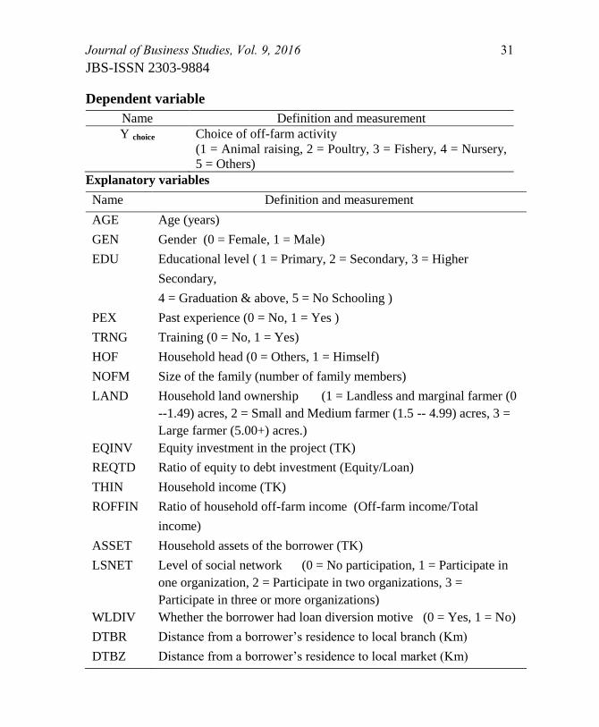
Dependent variable
Name Definition and measurement
Y choice Choice of off-farm activity
(1 = Animal raising, 2 = Poultry, 3 = Fishery, 4 = Nursery,
5 = Others)
Explanatory variables
Name Definition and measurement
AGE Age (years)
GEN Gender (0 = Female, 1 = Male)
EDU Educational level ( 1 = Primary, 2 = Secondary, 3 = Higher
Secondary,
4 = Graduation & above, 5 = No Schooling )
PEX Past experience (0 = No, 1 = Yes )
TRNG Training (0 = No, 1 = Yes)
HOF Household head (0 = Others, 1 = Himself)
NOFM Size of the family (number of family members)
LAND Household land ownership (1 = Landless and marginal farmer (0
--1.49) acres, 2 = Small and Medium farmer (1.5 -- 4.99) acres, 3 =
Large farmer (5.00+) acres.)
EQINV Equity investment in the project (TK)
REQTD Ratio of equity to debt investment (Equity/Loan)
THIN Household income (TK)
ROFFIN Ratio of household off-farm income (Off-farm income/Total
income)
ASSET Household assets of the borrower (TK)
LSNET Level of social network (0 = No participation, 1 = Participate in
one organization, 2 = Participate in two organizations, 3 =
Participate in three or more organizations)
WLDIV Whether the borrower had loan diversion motive (0 = Yes, 1 = No)
DTBR Distance from a borrower’s residence to local branch (Km)
DTBZ Distance from a borrower’s residence to local market (Km)
32 Journal of Business Studies, Vol. 9, 2016
JBS-ISSN 2303-9884
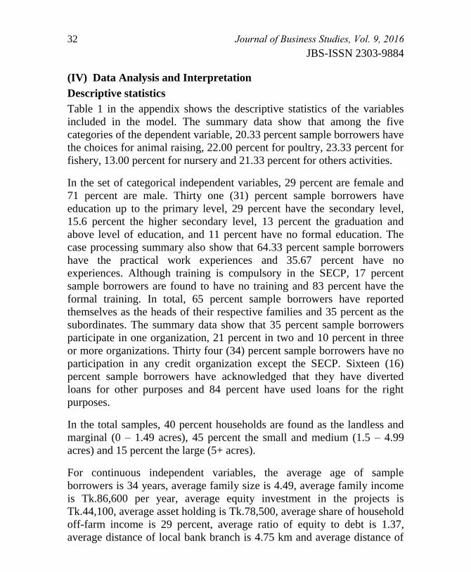
(IV) Data Analysis and Interpretation
Descriptive statistics
Table 1 in the appendix shows the descriptive statistics of the variables
included in the model. The summary data show that among the five
categories of the dependent variable, 20.33 percent sample borrowers have
the choices for animal raising, 22.00 percent for poultry, 23.33 percent for
fishery, 13.00 percent for nursery and 21.33 percent for others activities.
In the set of categorical independent variables, 29 percent are female and
71 percent are male. Thirty one (31) percent sample borrowers have
education up to the primary level, 29 percent have the secondary level,
15.6 percent the higher secondary level, 13 percent the graduation and
above level of education, and 11 percent have no formal education. The
case processing summary also show that 64.33 percent sample borrowers
have the practical work experiences and 35.67 percent have no
experiences. Although training is compulsory in the SECP, 17 percent
sample borrowers are found to have no training and 83 percent have the
formal training. In total, 65 percent sample borrowers have reported
themselves as the heads of their respective families and 35 percent as the
subordinates. The summary data show that 35 percent sample borrowers
participate in one organization, 21 percent in two and 10 percent in three
or more organizations. Thirty four (34) percent sample borrowers have no
participation in any credit organization except the SECP. Sixteen (16)
percent sample borrowers have acknowledged that they have diverted
loans for other purposes and 84 percent have used loans for the right
purposes.
In the total samples, 40 percent households are found as the landless and
marginal (0 – 1.49 acres), 45 percent the small and medium (1.5 – 4.99
acres) and 15 percent the large (5+ acres).
For continuous independent variables, the average age of sample
borrowers is 34 years, average family size is 4.49, average family income
is Tk.86,600 per year, average equity investment in the projects is
Tk.44,100, average asset holding is Tk.78,500, average share of household
off-farm income is 29 percent, average ratio of equity to debt is 1.37,
average distance of local bank branch is 4.75 km and average distance of
Journal of Business Studies, Vol. 9, 2016 33
JBS-ISSN 2303-9884
local market from home is 1.38 km. Total 300 cases were processed in the
analysis and there were no missing cases.
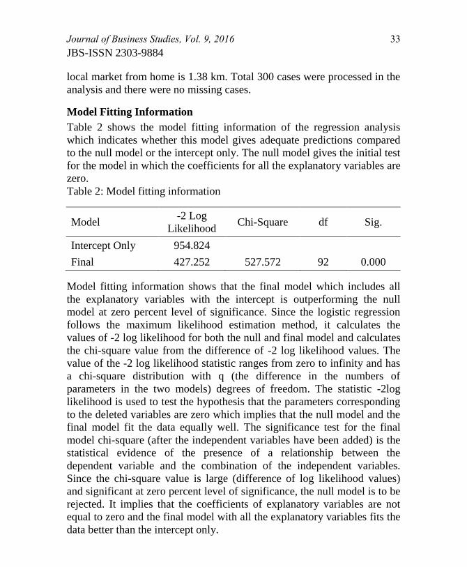
Model Fitting Information
Table 2 shows the model fitting information of the regression analysis
which indicates whether this model gives adequate predictions compared
to the null model or the intercept only. The null model gives the initial test
for the model in which the coefficients for all the explanatory variables are
zero.
Table 2: Model fitting information
Model -2 Log
Likelihood Chi-Square df Sig.
Intercept Only 954.824
Final 427.252 527.572 92 0.000
Model fitting information shows that the final model which includes all
the explanatory variables with the intercept is outperforming the null
model at zero percent level of significance. Since the logistic regression
follows the maximum likelihood estimation method, it calculates the
values of -2 log likelihood for both the null and final model and calculates
the chi-square value from the difference of -2 log likelihood values. The
value of the -2 log likelihood statistic ranges from zero to infinity and has
a chi-square distribution with q (the difference in the numbers of
parameters in the two models) degrees of freedom. The statistic -2log
likelihood is used to test the hypothesis that the parameters corresponding
to the deleted variables are zero which implies that the null model and the
final model fit the data equally well. The significance test for the final
model chi-square (after the independent variables have been added) is the
statistical evidence of the presence of a relationship between the
dependent variable and the combination of the independent variables.
Since the chi-square value is large (difference of log likelihood values)
and significant at zero percent level of significance, the null model is to be
rejected. It implies that the coefficients of explanatory variables are not
equal to zero and the final model with all the explanatory variables fits the
data better than the intercept only.
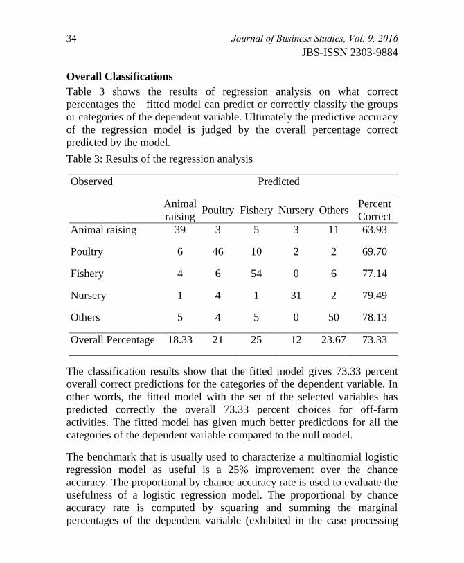
34 Journal of Business Studies, Vol. 9, 2016
JBS-ISSN 2303-9884
Overall Classifications
Table 3 shows the results of regression analysis on what correct
percentages the fitted model can predict or correctly classify the groups
or categories of the dependent variable. Ultimately the predictive accuracy
of the regression model is judged by the overall percentage correct
predicted by the model.
Table 3: Results of the regression analysis
Observed Predicted
Animal
raising Poultry Fishery Nursery Others
Percent
Correct
Animal raising 39 3 5 3 11 63.93
Poultry 6 46 10 2 2 69.70
Fishery 4 6 54 0 6 77.14
Nursery 1 4 1 31 2 79.49
Others 5 4 5 0 50 78.13
Overall Percentage 18.33 21 25 12 23.67 73.33
The classification results show that the fitted model gives 73.33 percent
overall correct predictions for the categories of the dependent variable. In
other words, the fitted model with the set of the selected variables has
predicted correctly the overall 73.33 percent choices for off-farm
activities. The fitted model has given much better predictions for all the
categories of the dependent variable compared to the null model.
The benchmark that is usually used to characterize a multinomial logistic
regression model as useful is a 25% improvement over the chance
accuracy. The proportional by chance accuracy rate is used to evaluate the
usefulness of a logistic regression model. The proportional by chance
accuracy rate is computed by squaring and summing the marginal
percentages of the dependent variable (exhibited in the case processing

Journal of Business Studies, Vol. 9, 2016 35
JBS-ISSN 2303-9884
summary). Therefore, the proportional by chance accuracy rate of the
model is 25.82 percent (1.25 x 20.65 % = 25.82 %). The classification
accuracy rate of the fitted model is 73.33 percent which is much greater
than the proportional by chance accuracy criteria of 25.82 percent.
Therefore the classification accuracy as well as the adequacy of the fitted
model is satisfactory in this analysis.
Measures of Effect Size or Pseudo R-Square
Table 4 shows that the measurement of effect size or the proportion of
variation explained by the fitted model. There is no widely-accepted direct
analogy to the R2 of OLS regression. The R-squared measures for logistic
regression cannot be compared directly with the R2 of OLS. Nonetheless, a
number of logistic R-squared measures may give an approximation to OLS
R2, not as actual percent of variance explained.
Table 4: Results of Pseudo R-Square
Pseudo R-Square
Cox and Snell 0.828
Nagelkerke 0.864
McFadden 0.553
Likelihood Ratio Tests
Table 5 in the appendix shows the results of the likelihood ratio test of the
logistic regression. The level of significance of each variable indicates
whether the variable has significant overall relationship with the
dependent variable. Results show that all the selected independent
variables are statistically significant at less than ten percent level of
significance. Therefore, the results of the likelihood ratio test indicate that
the independent variables included in the model have significant overall
relationship with the dependent variable.
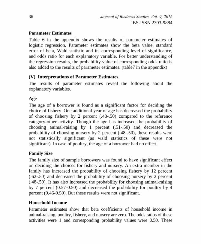
36 Journal of Business Studies, Vol. 9, 2016
JBS-ISSN 2303-9884
Parameter Estimates
Table 6 in the appendix shows the results of parameter estimates of
logistic regression. Parameter estimates show the beta value, standard
error of beta, Wald statistic and its corresponding level of significance,
and odds ratio for each explanatory variable. For better understanding of
the regression results, the probability value of corresponding odds ratio is
also added to the results of parameter estimates. (table7 in the appendix)
(V) Interpretations of Parameter Estimates
The results of parameter estimates reveal the following about the
explanatory variables.
Age
The age of a borrower is found as a significant factor for deciding the
choice of fishery. One additional year of age has decreased the probability
of choosing fishery by 2 percent (.48-.50) compared to the reference
category-other activity. Though the age has increased the probability of
choosing animal-raising by 1 percent (.51-.50) and decreased the
probability of choosing nursery by 2 percent (.48-.50), these results were
not statistically significant (as wald statistics of these were not
significant). In case of poultry, the age of a borrower had no effect.
Family Size
The family size of sample borrowers was found to have significant effect
on deciding the choices for fishery and nursery. An extra member in the
family has increased the probability of choosing fishery by 12 percent
(.62-.50) and decreased the probability of choosing nursery by 2 percent
(.48-.50). It has also increased the probability for choosing animal-raising
by 7 percent (0.57-0.50) and decreased the probability for poultry by 4
percent (0.46-0.50). But these results were not significant.
Household Income
Parameter estimates show that beta coefficients of household income in
animal-raising, poultry, fishery, and nursery are zero. The odds ratios of these
activities were 1 and corresponding probability values were 0.50. These
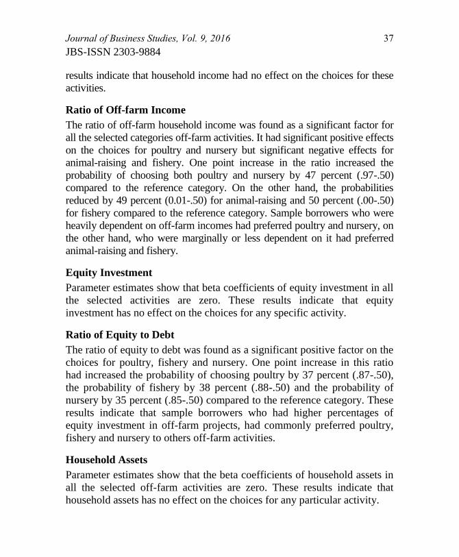
Journal of Business Studies, Vol. 9, 2016 37
JBS-ISSN 2303-9884
results indicate that household income had no effect on the choices for these
activities.
Ratio of Off-farm Income
The ratio of off-farm household income was found as a significant factor for
all the selected categories off-farm activities. It had significant positive effects
on the choices for poultry and nursery but significant negative effects for
animal-raising and fishery. One point increase in the ratio increased the
probability of choosing both poultry and nursery by 47 percent (.97-.50)
compared to the reference category. On the other hand, the probabilities
reduced by 49 percent (0.01-.50) for animal-raising and 50 percent (.00-.50)
for fishery compared to the reference category. Sample borrowers who were
heavily dependent on off-farm incomes had preferred poultry and nursery, on
the other hand, who were marginally or less dependent on it had preferred
animal-raising and fishery.
Equity Investment
Parameter estimates show that beta coefficients of equity investment in all
the selected activities are zero. These results indicate that equity
investment has no effect on the choices for any specific activity.
Ratio of Equity to Debt
The ratio of equity to debt was found as a significant positive factor on the
choices for poultry, fishery and nursery. One point increase in this ratio
had increased the probability of choosing poultry by 37 percent (.87-.50),
the probability of fishery by 38 percent (.88-.50) and the probability of
nursery by 35 percent (.85-.50) compared to the reference category. These
results indicate that sample borrowers who had higher percentages of
equity investment in off-farm projects, had commonly preferred poultry,
fishery and nursery to others off-farm activities.
Household Assets
Parameter estimates show that the beta coefficients of household assets in
all the selected off-farm activities are zero. These results indicate that
household assets has no effect on the choices for any particular activity.
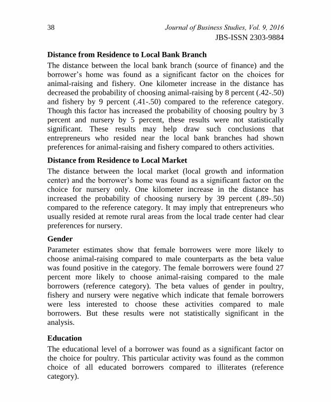
38 Journal of Business Studies, Vol. 9, 2016
JBS-ISSN 2303-9884
Distance from Residence to Local Bank Branch
The distance between the local bank branch (source of finance) and the
borrower’s home was found as a significant factor on the choices for
animal-raising and fishery. One kilometer increase in the distance has
decreased the probability of choosing animal-raising by 8 percent (.42-.50)
and fishery by 9 percent (.41-.50) compared to the reference category.
Though this factor has increased the probability of choosing poultry by 3
percent and nursery by 5 percent, these results were not statistically
significant. These results may help draw such conclusions that
entrepreneurs who resided near the local bank branches had shown
preferences for animal-raising and fishery compared to others activities.
Distance from Residence to Local Market
The distance between the local market (local growth and information
center) and the borrower’s home was found as a significant factor on the
choice for nursery only. One kilometer increase in the distance has
increased the probability of choosing nursery by 39 percent (.89-.50)
compared to the reference category. It may imply that entrepreneurs who
usually resided at remote rural areas from the local trade center had clear
preferences for nursery.
Gender
Parameter estimates show that female borrowers were more likely to
choose animal-raising compared to male counterparts as the beta value
was found positive in the category. The female borrowers were found 27
percent more likely to choose animal-raising compared to the male
borrowers (reference category). The beta values of gender in poultry,
fishery and nursery were negative which indicate that female borrowers
were less interested to choose these activities compared to male
borrowers. But these results were not statistically significant in the
analysis.
Education
The educational level of a borrower was found as a significant factor on
the choice for poultry. This particular activity was found as the common
choice of all educated borrowers compared to illiterates (reference
category).
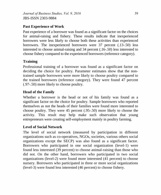
Journal of Business Studies, Vol. 9, 2016 39
JBS-ISSN 2303-9884
Past Experience of Work
Past experience of a borrower was found as a significant factor on the choices
for animal-raising and fishery. These results indicate that inexperienced
borrowers were less likely to choose both these activities than experienced
borrowers. The inexperienced borrowers were 37 percent (.13-.50) less
interested to choose animal-raising and 34 percent (.16-.50) less interested to
choose fishery compared to the experienced borrowers (reference category).
Training
Professional training of a borrower was found as a significant factor on
deciding the choice for poultry. Parameter estimates show that the non-
trained sample borrowers were more likely to choose poultry compared to
the trained borrowers (reference category). They were found 47 percent
(.97-.50) more likely to choose poultry.
Head of the Family
Whether a borrower is the head or not of his family was found as a
significant factor on the choice for poultry. Sample borrowers who reported
themselves as not the heads of their families were found more interested to
choose poultry. They were 45 percent (.95-.50) more likely to choose the
activity. This result may help make such observation that young
entrepreneurs were creating self-employment mainly in poultry farming.
Level of Social Network
The level of social network (measured by participation in different
organizations such as co-operatives, NGOs, societies, various others social
organizations except the SECP) was also found as a significant factor.
Borrowers who participated in one social organization (level-1) were
found less interested (39 percent) to choose animal-raising than those who
did not. On the other hand, borrowers who participated in two social
organizations (level-2) were found more interested (41 percent) to choose
nursery. Borrowers who participated in three or more social organizations
(level-3) were found less interested (46 percent) to choose fishery.

40 Journal of Business Studies, Vol. 9, 2016
JBS-ISSN 2303-9884
Diversion of Loan
The prior motive of loan diversion of a sample borrower was found as a
significant factor on the choices for poultry and fishery. Borrowers who
diverted loans for other purposes were 47 percent (.03-.50) less interested
to choose both these activities.
Household Land Ownership
The household land ownership of borrowers was found as a significant
factor on deciding the choices for fishery. Beta coefficients of the landless
& marginal farm households (from 0-1.49 acres of land) and the small &
medium farm households (from 1.5-4.9 acres of land) were negative in
fishery. These results indicate that both the landless & marginal and the
small & medium farm households were less likely to choose fishery
compared to large farm households (reference category). The landless &
marginal were 39 percent (.11-.50) and the small & medium were 42
percent (.08-.50) less interested to choose fishery. It clearly indicates that
only the large farm households have exclusive access to fishery.
(VI) Conclusions
Although the choice of a particular off-farm activity for self-employment
depends on both the motivation and the ability factors, the capacity of
households or individuals to participate in off-farm activities is not
uniform. Poverty, inequality in income and wealth, and human skills affect
the ability of an individual or household to engage in the preferred sector.
This study has identified some socio-economic ability factors found to
affect the decisions to engage in the selected off-farm activities. As many
as thirteen socio-economic ability factors of the SECP borrowers were
identified in five most preferred categories of off-farm activities by
borrowers in the study area. Table 8 below shows summary results of
those factors identified by parameter estimates of the fitted model of
logistic regression.
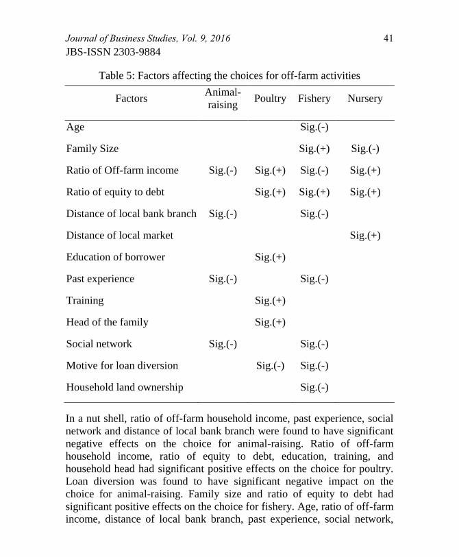
Journal of Business Studies, Vol. 9, 2016 41
JBS-ISSN 2303-9884
Table 5: Factors affecting the choices for off-farm activities
Factors Animal-
raising Poultry Fishery Nursery
Age Sig.(-)
Family Size Sig.(+) Sig.(-)
Ratio of Off-farm income Sig.(-) Sig.(+) Sig.(-) Sig.(+)
Ratio of equity to debt Sig.(+) Sig.(+) Sig.(+)
Distance of local bank branch Sig.(-) Sig.(-)
Distance of local market Sig.(+)
Education of borrower Sig.(+)
Past experience Sig.(-) Sig.(-)
Training Sig.(+)
Head of the family Sig.(+)
Social network Sig.(-) Sig.(-)
Motive for loan diversion Sig.(-) Sig.(-)
Household land ownership Sig.(-)
In a nut shell, ratio of off-farm household income, past experience, social
network and distance of local bank branch were found to have significant
negative effects on the choice for animal-raising. Ratio of off-farm
household income, ratio of equity to debt, education, training, and
household head had significant positive effects on the choice for poultry.
Loan diversion was found to have significant negative impact on the
choice for animal-raising. Family size and ratio of equity to debt had
significant positive effects on the choice for fishery. Age, ratio of off-farm
income, distance of local bank branch, past experience, social network,
42 Journal of Business Studies, Vol. 9, 2016
JBS-ISSN 2303-9884
loan diversion, and household land ownership had significant negative
effects for fishery. Ratio of off-farm income, ratio of equity to debt, and
distance of local market were found to have significant positive effects on
the choice for nursery but family size had significant negative effect on the
choice for nursery.
References
Davis, J. 2001, Conceptual Issues in analyzing the Rural Non-Farm
Economy in Transition Economies. NRI Social and Economic
Series. Report No. 2635.
Davis, J. 2003, The Rural Non-Farm Economy, livelihoods and their
diversification: Issues and options, Report No 2753, Natural
Resources Institute, UK.
Davis, J. and A. Gaburici 2001, Non-farm Employment in Small-Scale
Enterprises in Romania: Policy and Development Issues, NRI
Report No. 2637, Chatham: NRI.
Davis, J. and Cristoiu, A. 2002, Patterns of rural non-farm diversification
and employment in Romania: A county level analysis. NRI Social
and Economic Series Report No. 2639.
Davis, J., Pearce, D. 2001, The Non-Agricultural Rural Sector in Central
and Eastern Europe, Report No 2630, Natural Resources Institute,
UK.
Davis, J.R. and Bezemer, D.J., 2004, Key emerging and conceptual issues
in the development of the rural non-farm economy in developing
countries and transition economies. Report 2, DFID unpublished
mimeo.
NRI RNFE Project Team, 2000, (Marsland, N., Robinson, E., Davis, J.,
gordon, A. and Long, S.) Policy and Research on the Rural Non-
farm Economy: A Review of Conceptual, Methodological and
Practical Issues. Chatham, UK: Natural Resources Institute. Draft
Report.
Journal of Business Studies, Vol. 9, 2016 43
JBS-ISSN 2303-9884
Reardon T, Stamoulis K, Cruz M-E, Balisacan A, Berdegue J and Banks B
1998, Rural Non-Farm Income in Developing Countries. The state
of food and agriculture: Part III Rome, Food and Agricultural
Organisation of the United Nations.
Reardon, T., Berdegué, J. and G. Escobar 2001, Rural non-farm
employment and incomes in Latin America: Overview of issues,
patterns and determinants, World Development, 29 (3), March.
Reardon, T., Delgado, C. and Matlon, P. 1992, Determinants and effects of
income diversification amongst farm households in Burkina Faso.
Journal of Development Studies, 28: 264–296.
Reardon, T., E. Crawford, and V. Kelly. 1994. Links between non-farm
income and farm investment in African Households: adding the
capital market perspective, American Journal of Agricultural
Economics, Volume 76, No. 5 (December): 1172-1176.
Reardon, T., JE Taylor, K. Stamoulis, P. Lanjouw, A. Balisacan. 2000.
Effects of Non-farm Employment on Rural Income Inequality in
Developing Countries: An Investment Perspective, Journal of
Agricultural Economics 51(2), May: 266-288.
Reardon, T., P. Matlon, and C. Delgado. 1988. Coping with household-
level food insecurity in drought-affected areas of Burkina Faso,
World Development, Vol 16, No.9: 1065-1074.
Ellis, F. 1998, Household strategies and rural livelihood diversification,
Journal of Development Studies Vol.35, No.1, pp.1-38.
Ellis, F. 1999, Rural Livelihood Diversity in Developing Countries:
evidence and policy implications. Overseas Development Institute,
Natural Resource Perspectives, No.40. London: Overseas
Development Institute.
Ellis, F. 2000a, Rural Livelihoods and Diversity in Developing Countries.
Oxford: Oxford University Press Ellman, M.J. (2000)
Ellis, F. 2000b, The Determinants of Rural Livelihood Diversification in
Developing Countries. Journal of Agricultural Economics Vol. 51
(2): 289-302.
44 Journal of Business Studies, Vol. 9, 2016
JBS-ISSN 2303-9884
Ellis, F. 2000c, Survey Article: Household Strategies and Rural
Livelihood Diversification, Journal of Development Studies, 35(1):
1-38.
Ellis, Frank & Godfrey Bahiigwa, 2001, Livelihoods and rural poverty
reduction in Uganda, LADDER Working Paper No 5, November
2001, Overseas Development Group, University of East Anglia,
Norwich, UK
Ellis, Frank & Ntengua Mdoe, 2001, Livelihoods and rural poverty
reduction in Tanzania, LADDER Working Paper No 11, February
2001, Overseas Development Group, University of East Anglia,
Norwich, UK
Barret, C., Reardon, T., and Webb, P., 2001. Non-farm Income
Diversification and Household Livelihood Strategies in Rural
Africa: Concepts, Dynamics, and Policy Implications. Food Policy,
26: 315-31.
Barrett, C., and Reardon, T., 2000, Asset, Activity, and Income
Diversifications among African Agriculturalist: Some Practical
Issues, project report to USAID BASIS CRSP, March 2000.
Carney, D. 1998, Implementing the sustainable rural livelihoods approach.
pp. 3–23. In: Sustainable Rural Livelihoods – What Contribution
Can We Make? CARNEY, D. (ed.). London: Department for
International Development.
Journal of Business Studies, Vol. 9, 2016 45
JBS-ISSN 2303-9884
The Economics of Price Volatility in Commodity Futures
Markets: A Survey
Mahmud Hossain Riazi
Abstract
This paper reviews the major contributions concerning commodity futures
markets with special attention paid to the dynamics of futures price volatility.
With the turn of the century, there has been a considerable shift in the subject
matter of volatility literature, the preponderance of the issues of seasonality being
the rather significant phenomenon than the previous research works. Keeping this
in mind, attempt has been made to compare and contrast the existing literatures
of volatility with its current trends and to identify what differences they entail in
their implications to deal with the more practical decision-making issues
regarding storage and hedging behaviour. In that pursuit, this paper addresses
both the theoretical and empirical literatures on futures price volatility and
critically examines them in terms of some more detailed topics like what
commodities they analyze, what models they employ, what techniques they use
for data construction and so on. The discussion will likely to trigger new research
insight in the field of futures price volatility.
Keywords: Commodity futures, volatility, seasonality, time-to-maturity, storage
theory, term-structure models, hedging
(I) Introduction
here is an extensive body of literature on the behaviour of commodity
futures prices. The main aspects of this literature are articulated and
discussed in the review articles of Carter (1999), Gray and Routledge
(1971), Kamara (1982), Blank (1989), Milliaris (1997), Garcia and
Leuthold (2004) and Lautier (2005). The critical areas of research that
dominate this vast literature can be classified into several broad categories:
(i) the issues in price discovery and efficiency of futures market (ii) the
analysis of term-structure of commodity futures price that aims to evaluate
the commodity related derivatives (iii) the identification of nature and
Associate Professor, Department of Economics, University of Rajshahi,
Email: [email protected]
T
46 Journal of Business Studies, Vol. 9, 2016
JBS-ISSN 2303-9884
causes of volatility of futures prices and (iv) the theories and empirical
issues in hedging that devise the effective ways of risk management.
With the growth of futures markets, the scope of research on commodity
futures prices has changed significantly during the recent years. The centre
of attention has been to capture, as precisely as possible, the stochastic
behaviour of commodity prices which play a central role for pricing
commodity contingent claims and quantifying their inherent volatility
structure (Schwartz, 1997). To this end, different latent factor models are
employed to determine the term-structure of commodity futures (and
option) prices and their volatility. In addition to this, different time-
varying volatility models for analyzing the volatility dynamics of
commodity prices have been used. These models require complex
mathematical algorithms, and sometimes, numerical techniques for their
solution because the storability of most commodities and their inherent
seasonality in the production or (and) consumption process cause their
stochastic dynamic system to be non-linear. The solutions of the dynamic
systems for futures prices and their volatility enable different economic
agents, especially the hedgers, to manage risk in an effective way.
This paper critically reviews the streams of empirical literature on the
nature and causes of commodity price volatility, especially, the volatility
of agricultural futures prices. However, before going to the thorough
analysis on this topic, the traditional term-structure models deserve a brief
discussion because these models have important implications for hedging
and analyzing seasonality. The effectiveness of an empirical model of
commodity price behaviour depends, to a great extent, on two vital issues:
first, how well this model fits the real world commodity price data and
secondly, and more importantly, how consistent the model is with the
underlying theories that guide the commodity price behaviour.
Accordingly, prior to analyzing the comparative analysis of the
commodity price models a brief analysis of the basic theories of
commodity prices is required.
The organization of this paper is as follows. Section (ii) describes the main
theories of commodity price and their main empirical tests. Section (iii)
analyzes the standard term-structure models. The previous research on the
Journal of Business Studies, Vol. 9, 2016 47
JBS-ISSN 2303-9884
volatility of futures prices and their determinants are addressed in section
(iv). Section (v) presents some modelling issues in volatility literature.
Section (vi) reviews the literature on hedging and Section (vii) concludes.
(II) Basic Theories of Commodity Prices
The theory of storage (Kaldor 1940; Working 1949) and the theory of
normal backwardation (Keynes 1923; Hicks 1946) have been embraced as
the two most important theories of commodity price behaviour (Fama and
French, 1987). However, recently the focus of research has been shifted to
a great extent to the theory of storage in a rational expectation setting that
suits best for the explanation of the term-structure of volatility.
Theory of normal backwardation and its empirical test
The theory of normal backwardation explains the relationship between
spot and futures prices in terms of the function of transferring risk. The
theory of normal backwardation states that, in a normal situation, the
commodity markets are characterized by a forward price lying below the
spot price. Central to the analysis of normal backwardation is the existence
of a positive risk premium in futures market contracts. As speculators sell
insurance to the hedgers, the former should receive a positive risk
premium (often called the Keynes-Hicks risk premium) from the later and
this risk premium equals the difference between spot and futures price at
the contract delivery date.
There has been much empirical testing of the theory of normal
backwardation that led to much controversy and debate. It has never been
truly validated nor rejected. Telser (1958) tests the theory of normal
backwardation and rejects it. Cootner (1960), on the other hand, finds
evidence for this theory. Later, Dusak (1973) and Bessembinder (1993)
use the capital asset pricing model to test the presence of risk premia in
futures contracts. Dusak uses futures on wheat, corn and soybeans whereas
Bessembinder uses agricultural futures on live cattle, soybeans, sugar,
wheat, cotton and corn. They conclude that risk premium is not positive
for all commodities. It might be zero or sometimes negative leading to
normal contango. Kolb (1992) analyzes 29 futures contracts (16
agricultural commodities, 4 foreign exchanges, 2 energy futures, 2 bonds,
5 precious metals) and finds evidence against the existence of risk premia.
48 Journal of Business Studies, Vol. 9, 2016
JBS-ISSN 2303-9884
In contrast, Fama and French (1987) analyze 21 commodities1 and find
evidence in favour of risk premia. Sorensen (2002) analyzes the term-
structure of corn, soybean and wheat prices and shows that normal
backwardation is valid for soybean and wheat, whereas the case is mixed
for corn with normal backwardation valid for long contract maturities and
contango valid for short contract maturities.
Theory of storage and its empirical tests
The theory of storage explains the relationship between the spot and the
futures price of a commodity in terms of convenience yield, a stream of
implicit revenue associated with the stock of physical holding of the
commodity. Brennan and Schwartz (1985) define convenience yield as the
“flow of services that accrues to an owner of the physical commodity but
not to the owner of a contract”. Kaldor (1940) proposes this theory which
has subsequently been elaborated by Working (1948, 1949), Telser (1958),
Williams (1989), and Brennan (1991). This theory posits that the marginal
value of convenience yield declines as inventory increases and becomes
zero for high inventory level. This inverse relationship is sometimes called
the Kaldor-Working hypothesis. The cost of carrying stocks from one
date to another determines inter-temporal price relation.
A positive convenience yield, through arbitrage, depresses the futures
price relative to spot price (Ng and Pirrong, 1994). This is evident from
the no arbitrage relation between the spot and the futures prices is:
where, is the futures price at t to be delivered at time T, is the spot
price at t, is the physical storage cost during the time span between t
to T, is the interest rate and is the convenience yield. This
1 Ten agricultural commodities (cocoa, coffee, corn, cotton, oats, orange juice, soybeans,
soy meal, soy oil and wheat), two wood products (lumber and plywood), five animal
products (broilers, eggs, cattle, hogs and pork bellies) and four metals (copper, gold,
platinum and silver).

Journal of Business Studies, Vol. 9, 2016 49
JBS-ISSN 2303-9884
relationship can be expressed in terms of interest and storage adjusted
spread as:
The spread is inversely related to convenience yield and directly related to
inventory. This equation explains that the spread is below full carrying
charges and storage must be taken place at an opportunity cost, the
convenience yield. Using quarterly data from the United States
Department of Agriculture (USDA) on stocks of inventory, Sorensen
(2002) empirically validates the Kaldor-Working hypothesis for corn,
soybeans and wheat.
Modern version of the theory of storage
The modern version of the storage theory explains the relationship
between the spot and futures prices in terms of the interaction between
stock-out (depletion) and spread in a setting of a competitive storage
model based on rational expectations. Unlike the two theories mentioned
above, this modern theory of storage does not depend on the elusive
concepts like convenience yield or risk premium to explain the prevalence
of spread below full carrying charge in grain futures markets. Rather, it
uses the simple supply-demand fundamentals. This theory originates with
the pioneering work of Gustafson (1958), who explicitly assumes the
impossibility of carrying forward negative inventory, and Muth (1961),
who introduces the assumption of rational expectation2 in the competitive
storage model. Subsequently, Wright and Williams (1982) and Williams
and Wright (1991) formally elaborate the model.
The point of departure for the analysis of storage theory is the dual role
played by storage itself on the time series behaviour of the storable
2 By rational expectation is meant that the producers and the storers in the competitive
storage model are able to make objective calculations about the probability distribution of
yields and price response to the inevitable production shocks (Williams and Wright,
1991).

50 Journal of Business Studies, Vol. 9, 2016
JBS-ISSN 2303-9884
commodity. The level of storage determined3 in the competitive storage
model has important price-smoothing properties; First, it can spread the
shocks of a good or bad harvest across a number of periods. Second, the
variance of price movement decreases as the amount of storage increases.
However, storage has an asymmetric effect on price as the price-
smoothing role of storage is limited only to supporting low prices rather
than lowering high prices. This asymmetry is attributed to the non-
negativity constraint on storage as private agents store only when there is
surplus, but, collectively, the market cannot borrow from the future.
The non-negativity constraint has significant implications for explaining
commodity price behaviour. The most important characteristics of
commodity (esp. the grains that are subject to seasonal harvesting) prices
is that they are mean-reverting and converge to a stochastic steady state in
the long-run. This phenomenon is the direct result of backwardation in
commodity prices and a spread below full carrying charges across a crop
year. The current shortage (very low or zero stockpile) leads to stock-outs,
increase spot price and thereby gives rise to backwardation in price. The
stock-out in turn increases the probability of having a small availability in
the next period. However, with a likelihood of successive replenishment of
stocks, the probability of stock-out in the distant periods will gradually
decrease and the spread will be below full carrying charges. This has been
empirically tested in the work of Deaton and Laroque (1992) for thirteen
commodities (bananas, cocoa, coffee, copper, cotton, jute, maize, palm oil,
rice, sugar, tea, tin, wheat) and Ng and Pirrong (1994) for four
commodities (copper, lead, silver and zinc).
The nature of volatility in commodity prices can also be seen in terms of
adjustment of stock. During the time of stock-out and shortage, the non-
negativity constraint does not allow the system to borrow from the future
which breaks the inter-temporal price linkage and price-smoothing role of
storage. Any minor shock can then create disproportionately large price
3 The level of storage and the price in each period are jointly determined in the
competitive storage model –the arbitrage activity of the storers based on rational
expectation determines the level of storage whereas the availability and storage rule
determine price in each period.

Journal of Business Studies, Vol. 9, 2016 51
JBS-ISSN 2303-9884
volatility in the system. This phenomenon has been empirically verified by
Suenaga, Smith and Williams (2008) for NYMEX (New York Mercantile
Exchange) natural gas futures and by Suenaga and Smith (2011) for
NYMEX crude oil, heating oil and unleaded gasoline futures.
(III) Price Volatility and the Term-Structure Models
The stochastic term-structure models of commodity prices play a central
role in evaluating commodity-related derivatives and real assets. They try
to reproduce the prices of the derivatives (futures or options on futures)
observed in the market. They also provide a means for the discovery of
futures prices for horizons exceeding exchange traded maturities (Lautier,
2005). These models usually specify the dynamics of the state variables
that are assumed to follow some specific stochastic processes. The
arbitrage reasoning and the construction of a hedging portfolio lead the
model to provide a valuation formula for futures prices. The difference
between the model-implied futures prices and the observed futures prices
are interpreted as representing the risk premium.
The basic ideas that give rise to the formation of term-structure models for
commodity prices are: Black and Scholes‟ (1973) option pricing model;
Cox, Ingersoll and Ross‟ (1981) term-structure models for interest rates;
and Vasicek‟s (1977) application of Ornstein-Uhlenbeck process for
interest rate dynamics. Gibson and Schwartz (1990), Brennan (1991),
Schwartz (1997) and Schwartz and Smith (2000) are the exponents who
successfully introduce and popularize the mean-reverting models for the
valuation of commodity-contingent claims. At the centre of the analysis of
term-structure models for commodity prices is the theory of storage
(Kaldor, 1940; Working, 1948, 1949; Telser, 1958; Brennan, 1958;
Williams, 1989; and Williams and Wright, 1991).
Depending on the number and nature of factors (state variables) and the
specific stochastic process that they are assumed to follow there have been
several types of term-structure models of commodity futures prices. The
spot price of a commodity is thought to be the principal determinant of its
futures price. This leads most one-factor models to suppose the spot price
52 Journal of Business Studies, Vol. 9, 2016
JBS-ISSN 2303-9884
to be the only factor, for example, Brennan and Schwartz (1985)4,
Schwartz (1997) and Cortazar and Schwartz (1997). Subsequently, in
order to capture a more realistic stochastic behaviour of commodity prices
a second factor, the convenience yield, is included.
Gibson and Schwartz (1990) and Schwartz and Smith (2000) are two basic
two-factor models that follow the approach of Cox, Ingersoll and Ross‟
(1981) for pricing commodity contingent claims. Gibson and Schwartz
(1990)5 are the first to assume that the convenience yield is
stochastic6 rather than constant and that it follows a mean-reverting
process. Specifically, the dynamics of spot price in this model follows a
geometric Brownian motion. One problem of this model is it does not give
a closed-form solution for the futures prices. Rather, its parameters are
estimated by Seemingly Unrelated Regression (SUR) analysis.
4 Brennan and Schwartz (1985) assume that commodity spot price follows a geometric Brownian
motion (GBM). However, subsequently, many scholars (Dixit and Pindyck, 1994; Cortazar and
Schwartz, 1994; Bessembinder, 1995; Schwartz, 1997) prefer mean-reverting price models over the
GBM process. 5 The spot price of oil, S and the net convenience yield, follow a joint diffusion process
as:
where, and are the increments to standard Brownian motion, and are the
volatilities of spot price and convenience yield respectively and ρ is the correlation co-
efficient between the two Brownian motions. The spot price of oil follows a geometric
Brownian motion whereas the instantaneous convenient yield follows a mean-reverting
process5. As the data on the state variables cannot be observed, proxy variables are used
for them. Using the no-arbitrage argument the value of futures contract, can be
shown by solving a particular differential equation:
subject to the initial condition:
However, there is no closed-form solution for the futures price and so a numerical
technique is resorted to for computation of futures price. The parameters of the model are
estimated using the seemingly unrelated regression analysis using the NYMEX data on
crude oil.
6 Brennan and Schwartz (1985) assume a constant convenience yield.
Journal of Business Studies, Vol. 9, 2016 53
JBS-ISSN 2303-9884
Gibson and Schwartz (1990) inspire the formulation of a host of more
sophisticated models, for example, Schwartz (1997), Cortazar and
Schwartz (2003) and Hilliard and Reis (1998). Schwartz (1997) is the
most popular term-structure model of commodity price dynamic. Unlike
Gibson and Schwartz (1990), this model gives a closed-form solution for the commodity contingent claims and is mathematically tractable through
the use of Kalman filter technique. Cortazar and Schwartz (2003) devise a
three factor model which is an extension of a reformulated two-factor
model of Schwartz (1997). This model is more parsimonious than
Schwartz (1997) in terms of number of parameters needed to be estimated.
Hilliard and Reis (1998) extend Schwartz (1997) model in order to
introduce jumps in the spot price process so that it can capture sudden
supply and demand shocks. This model suits better for energy
commodities.
Schwartz and Smith (2000) criticize the Gibson and Schwartz (1990)
tradition for assuming equilibrium price, to which the short-run prices
revert, to be fixed. In contrast to Gibson and Schwartz (1990), they
decompose the spot price into two stochastic factors: the short-term
deviation in price and a long-run equilibrium price level which is assumed
to be uncertain. The short-run deviation in price follows a mean-reverting
process of the Ornstein-Uhlenbeck type7 whereas the long-run equilibrium
price level is assumed to follow a GBM process. This short-term/long-
term model gives a closed-form solution for the futures prices and is
exactly equivalent to the Gibson and Schwartz (1990) model8. This model
is the simplest form of the general affine9 term-structure models. This
model is very realistic and amenable to empirical analysis. First, it avoids
the estimation of convenience yield which is an „elusive‟ concept to many.
7 Uncertainty about the long-run price stems from changes in expectations about existing
supply, technological improvement regarding production and exploration of a
commodity, inflation or any regulation that can affect supply. Conversely, short-run
changes in price refer to any shock that limits the ability of the market to adjust inventory
levels to changing market conditions. 8 “The state variable in each model can be represented as linear combinations of the state
variables in the other” (Schwartz and Smith, 2000). 9 In this formulation, the logarithm of asset price is a linear function (affine function) of
latent (unobservable) state variables.
54 Journal of Business Studies, Vol. 9, 2016
JBS-ISSN 2303-9884
Second, the volatility of the futures price is easy to calculate. Third, this
model is parsimonious compared to Gibson and Schwartz (1990) and,
fourth, it can easily incorporate seasonal factor. Sorensen (2002) extends
the affine term-structure model to analyze seasonality in agricultural
commodities (corn, wheat and soybeans futures), whereas Todorova
(2004) applies this model for analyzing seasonality in crude oil and the
natural gas futures market. Subsequently, more complex affine models
have been set by Cassassus and Collin-Dufresne (2005), or in the
stochastic volatility model10
of Richter and Sorensen (2002).
Two-factor models have been extended later by different authors to get a
more precise model for explaining commodity price dynamics. Schwartz
(1997) includes a third factor, the stochastic interest rate. Manoliu and
Tompaidis (2002) introduce a multi-factor model, while Cortazar and
Schwartz (2003) introduce a third factor, long-term spot price return to the
reformulated Schwartz (1997) model. Hilliard and Reis (1998) introduces
a jump in the spot price process of Schwartz (1997) model. However,
there is always a trade-off between model performance and complexity of
the models. Schwartz (1997) compares performance between one-factor,
two-factor and three-factor models. Whereas two-factor model
outperforms one-factor model significantly, the three-factor model only
marginally improves the performance of two-factor models.
Although, the traditional term-structure models are very useful for pricing
commodity contingent claims and devising hedging strategies they have
limited practical use in explaining the pattern of commodity price
volatility. These models provide a crude measure of volatility dynamics of
futures prices that depends on time-to-delivery and the volatility
parameters of the state variables. They can only indicate the volatility of
futures prices to be a decreasing function of time-to-delivery. But, due to
the time-invariant nature of the volatility of state variables, the model
implied volatility measure is unable to explain the time-varying volatility
that stems from seasonality and other shocks in the economy. However,
10 The traditional term-structure models assume the volatility of the underlying state
variables to be constant, whereas in the stochastic volatility models the volatility of the
underlying state variables follows some stochastic process.
Journal of Business Studies, Vol. 9, 2016 55
JBS-ISSN 2303-9884
the affine term-structure model can incorporate seasonality and time-
varying volatility in the system (Sorensen, 2002; Richter and Sorensen,
2002).
(IV) Theories and Empirics on the Volatility of Futures Prices
Hypotheses on Price Volatility
Commodity prices, especially the prices of agricultural commodities, are
subject to high degrees of volatility. Production decisions and risk-
management require the producers, commodity traders and policy makers
to have good knowledge about the pattern and causes of price volatility of
agricultural commodities. The price variability of agricultural
commodities has been attributed to a number of factors: (a) Reactions to
information flows (Kyle, 1985; Anderson and Bollerslev, 1997); (b) Time-
to-delivery (Samuelson, 1965; Milonas, 1986; Castelino, 1982); (c)
Seasonality (Anderson, 1985; William and Wright, 1991); (d) Persistence
in volatility (Kenyon et al., 1987) and (e) Trade volume (Cornell, 1981;
Streeter and Tomek, 1992).
The most important hypothesis concerning the dynamic behaviour of
commodity prices is the time-to-maturity effect (Samuelson, 1965). This
hypothesis states that the movements of prices are large for short-term
contracts and small for long-term contracts, indicating that the volatility
exhibits a decreasing pattern along the price curve. As futures contracts
approach their expiration date and incorporate new information, they react
much more strongly to information shocks, due to the ultimate
convergence of futures prices to spot prices upon maturity.
Seasonality is the other source, and to many the biggest source, of
volatility for most agricultural (and energy) commodities. According to
this view, seasonality lies behind the interaction of real economic
variables: very low inventory at the end of the production cycle together
with the impossibility of borrowing from the future break the inter-
temporal arbitrage link of storage. For some commodities, this response to
low inventory is attributed to the inelastic nature of the demand curve, for
example, natural gas in winter (Suenaga, Smith and Williams, 2008). For
other commodities this is the result of both inelastic demand and supply
curve, for example, the commodities that are complementary in production
56 Journal of Business Studies, Vol. 9, 2016
JBS-ISSN 2303-9884
but subject to different timing of consumption, such as heating oil and
unleaded gasoline (Suenaga and Smith, 2011).
Empirical Studies on time-to-maturity and seasonality
The time-to-maturity and seasonality effects have been subject to many
empirical tests. Rutledge (1976) examines daily price movements of
silver, cocoa, wheat and soybean contract, respectively, from Commodity
Exchange Incorporated of New York (COMEX), New York Cocoa
Exchange, Kansas City Board of Trade (KC) and Chicago Board of Trade
(CBOT). He rejects the Samuelson hypothesis for wheat and soybean oil,
but accepts it for cocoa. Miller (1979) uses logarithms of the daily closing
price and analyses June and December live beef contracts of the Chicago
Mercantile Exchange (CME) for 1964-1972. She finds no support for the
time-to-maturity effect. Castelino (1982) uses daily data of wheat, corn,
soybeans, soybean meal and soybean oil contracts at CBOT and copper at
COMEX over 1960-1971. The result supports the Samuelson hypothesis.
Anderson (1985) tests both time-to-maturity and the state variable
hypothesis11
for seven agricultural commodities (wheat, corn, oats,
soybeans, soybean oil, cocoa and live cattle) and a metal, silver. The tests
shows that time-to-maturity effect and the state variable hypothesis can
hold at the same time. Besides, for most of the commodities seasonality
effect exceeds maturity effect. The secondary factor is the time-to-
maturity. The other important finding of his study is that the time-to-
maturity holds only for daily price data.
Milonas (1986) provides empirical support for the time-to-maturity effect
for a large number of commodities. On the other hand, Deaton and
Laroque (1992) and Chambers and Bailey (1996) show that Samuelson
effect is a function of storage cost. A high storage cost leads to less
transmission of shocks via inventory across periods and so volatility of
futures price declines rapidly with maturity.
11 State variable hypothesis relates volatility with the supply-demand state variables.
When uncertainty regarding the state variables is resolved, prices incorporate new
information which leads to price volatility. According to the state variable hypothesis,
this process of new information generation at the maturity of a contract is itself seasonal
(Stein, 1979; Anderson and Danthine, 1983).
Journal of Business Studies, Vol. 9, 2016 57
JBS-ISSN 2303-9884
Khoury and Yourougou (1993) use daily data on canola, rye, feed barley,
feed wheat, flaxseed and oats from the Winnipeg Commodity Exchange
and test the determinants of volatility. The results show that the price
volatility is affected by the year, calendar month, contract month, time-to-
maturity and trading session effects. Kenyon, et al (1987) analyze five
agricultural commodities: soybean, corn, wheat, live cattle and live hogs,
and find that grain price volatility is affected by seasons and level of
futures price relative to loan rate.
Yang and Brorsen (1993) use a GARCH (1, 1) model to test the effect of
day-of-the-week, time-to-maturity and seasonality on the basis values of
15 different futures prices (7 grains, 5 metals and 3 financial futures).
There is a significant day-of-the-week effect: Mondays have higher
variance and Wednesdays have lower variances, so the results favour the
calendar time hypothesis over the trading time hypothesis. Also,
agricultural futures prices show seasonality in their variance. Streeter and
Tomek (1992) find that the time-to-maturity has a non-linear effect on
price volatility, the volatility decreases in the month before maturity.
However, there is a strong relationship between seasonality and volatility
of soybean futures prices. Hennessy and Wahl (1996) show that
seasonality affects the price volatility of corn, soybean and wheat.
However, there is no influence of time-to-maturity on volatility.
There are many recent empirical studies on the effect of seasonality and
time-to-maturity on the behaviour of commodity futures prices. Manoliu
and Tompaidis (2002); Suenaga, Smith and Williams (2008); Suenaga and
Smith (2011) are significant studies on energy related commodities. On
the other hand, Goodwin and Schnepf (2000); Sorensen (2002); Richter
and Sorensen (2002); Chatrath, Adrangi and Dhanda (2002); Schaefer,
Myers and Koontz (2004); Smith (2005); Kalev and Duong (2008); Karali,
Dorfman, Thurman (2010); Karali and Thurman (2010); Ovararin and
Meade (2010) conduct research on seasonality in agriculture.
Sorensen (2002) analyzes the stochastic behaviour of agricultural
commodity prices under seasonality using CBOT weekly futures price
data of corn, soybean and wheat. This adds a seasonal component to the
short-term/long-term model of Schwartz and Smith (2000). The estimated
58 Journal of Business Studies, Vol. 9, 2016
JBS-ISSN 2303-9884
seasonal parameters show that this model fits the CBOT agricultural
futures data better than the Schwartz and Smith (2000). For all three
commodities the estimated seasonal components peak two or three months
before the beginning of US harvest. However, this effect is less
pronounced for soybeans due to the bulk supply of soybeans in the US
market from the Southern hemisphere. On the other hand, the falling
standard deviation of the futures prices with increasing time-to-maturity, a
positive mean-reverting parameter for the stationary state variable and a
smaller value of the estimated volatility parameter for non-stationary
component than the stationary component suggest that the data supports
Samuelson hypothesis.
Manoliu and Tompaidis (2002) add a deterministic seasonal component to
a multi-factor model within the Heath, Jarrow and Morton (1992)
framework and test it with NYMEX daily natural gas futures price. The
estimated model exhibits a strong seasonal variation in price, with a higher
monthly seasonality index for winter months and a lower seasonality index
for summer months. Richter and Sorensen (2002) use the weekly soybean
futures price from CBOT and analyze the effect of seasonality in soybean
futures and options. They extend the Gibson and Schwartz (1990) model
with an additional factor, a stochastic volatility term, and add two
deterministic trigonometric seasonal functions to it, one for the
convenience yield and the other for the stochastic volatility term12
. They
12 As in Gibson and Schwartz (1990), the convenience yield follows a mean-reverting process. If Pt,
δt and υt denote respectively the three state variables – spot commodity price, convenience yield
and seasonally adjusted spot price volatility – the dynamics of the three dimensional process (P, δ,
υ) can be described by a system of stochastic differential equations:
where, β, κ, θ, λP, λδ, λυ, σδ, συ are constant parameters to be estimated. W = (W1, W2, W3) is the
three-dimensional Wiener process where the Ws are assumed correlated one another with
correlation coefficients ρ12, ρ13 and ρ23. The parameters β and κ are the degree of reversion to the
deterministic seasonal pattern in convenience yield and long-run volatility level, θ, respectively.
The parameters λP, λδ, and λυ are respectively the risk premia on uncertainty of commodity price,
convenience yield and volatility. The parameters σδ, συ denote volatility of convenience yield and
stochastic volatility of commodity price, respectively.
The functions α(t) and ν(t) show seasonal patterns in convenience yield and volatilities
and are specified by trigonometric functional forms. In the first two equations, both the changes in
Journal of Business Studies, Vol. 9, 2016 59
JBS-ISSN 2303-9884
find high price volatility (a global maximum in the seasonal function) in
soybean prices before US soybean harvest (July). On the other hand,
soybean volatility is low in March before US planting (in May and June).
Besides, the volatility process shows considerable mean-reversion and is
consistent with the theory of storage.
Chatrath, Adrangi and Dhanda (2002) find that daily returns on soybean,
corn, wheat and cotton are highly dependent on seasonality. Besides,
soybean and corn support the time-to-maturity effect. Kalev and Duong
(2008) analyze eight commodities (corn, soybean, soybean oil, soybean
meal, feeder cattle, lean hogs, live cattle and pork bellies) and find
evidence of a time-to-maturity effect.
Smith (2005) uses partially overlapping time-series (POTS)13
model and
performs an empirical test of the theory of storage and the Samuelson
effect with CBOT corn futures price data. The resulting high value in the
proportion of model variance explained by the common factors,
, gives an indication that suggests the data support the
theory of storage. On the other hand, a high proportion of old crop
variance to new crop variance strongly supports a low correlation between
factors and thereby a break in the relation between nearby and distant
futures prices, a backwardated price and low inventory. This model also
supports the time-to-maturity effect.
Suenaga, Smith and Williams (2008) show that highly non-linear volatility
dynamics of natural gas futures prices are attributed to strong seasonality
in demand and storage as well as the time-to-maturity. Their analysis is
built on the principles of storage theory. Using the POTS model of Smith
(2005) in a single-factor setting they analyse the NYMEX data on natural
gas futures price. They argue that both inelastic winter demand and high
spot prices and convenience yield are affected by the same seasonality pattern because seasonality
influences both variables through storage.
Futures price can be found by using the Feynman-Kac formula:
There is no closed-form solution for the futures price.
13 The POTS model is presented in sub-section 5.1
60 Journal of Business Studies, Vol. 9, 2016
JBS-ISSN 2303-9884
storage cost peculiar to natural gas reduce inventory level and thereby
limit the price-smoothing property of inventory during winter. Any
information shock about winter gas availability, which normally comes
during the preceding off-peak season (May-September), causes the prices
of winter futures contract to be highly volatile. On the other hand, the
price of early winter futures contract is less volatile as inventory keeps
piling up in this period. That the above pattern of seasonality in price
volatility is consistent with the theory of storage is further supported by
the seasonal pattern of US nationwide gas storage data.
Suenaga and Smith (2011) use the POTS model of Smith (2005) and
analyze the volatility dynamics in the price of three petroleum
commodities – crude oil, unleaded gasoline and heating oil. Using
NYMEX futures price data, they find strong seasonality and time-to-
maturity effects in the highly non-linear volatility pattern of futures prices.
Ovararin and Meade (2010) use daily closest futures prices of rubber, rice
and sugar and test for mean-reversion and seasonality in volatility. They
consider two types of seasonalities: a day-of-the-week seasonality, which
represents investor‟s behaviour, and a yearly seasonality, which
demonstrates the effect of the harvest. A GARCH (1, 1) model is extended
thrice with trigonometric deterministic seasonal functions that capture
mean-reversion, day-of-the-week effect and yearly seasonality. The
estimated results show that the daily return process for the three
commodities are not mean reverting but show day-of-the-week effect and
annual seasonality. Karali and Thurman (2010) study the effect of time-to-
maturity, seasonality, calendar trend and volatility persistence using
CBOT multiple contracts on corn, soybeans, wheat and oats traded each
day. They apply the generalized least square method of Karali and
Thurman (2009) and estimate the model parameters by seemingly
unrelated regression analysis. The study strongly supports the time-to-
maturity effect and seasonality in the pattern of price volatility. The
volatility peaks in the summer, just two months before the harvest.
(V) Issues in Volatility Modelling
This section presents some technical issues that are crucial for volatility
modelling. Basically three issues are stressed here: (i) a comparison
Journal of Business Studies, Vol. 9, 2016 61
JBS-ISSN 2303-9884
between models in terms of their relative advantages and disadvantages
(ii) issues in data arrangement (iii) different methods for modelling
seasonality.
Types of Volatility models
The models that are popular for volatility analysis are briefly discussed in
this sub-section. Six models are widely seen in this case.
(a) Constant volatility models for the analysis of commodity contingent
claims (Sorensen, 2002; Manoliu and Tompaidis, 2002).
(b) Historical volatility models in which the volatility is estimated based
on previous historical standard deviation.
(c) Autoregressive conditional heteroskedastic models(ARCH) and
Generalized ARCH (GARCH) models (Yang and Brorsen, 1993;
Ovararin and Meade, 2010)
(d) Stochastic volatility (SV) models (Richter and Sorensen, 2002)
It differs from GARCH model in that the conditional variance in a
stochastic volatility model itself depends on a stochastic process.
(e) Implied standard deviation or (ISD) models
This is the volatility implied by the Black-Scholes option pricing
model.
(f) Partially overlapping time-series analysis (POTS) (Smith, 2005;
Suenaga, Smith and Williams 2008; Suenaga and Smith 2011)
The last model is comparatively new and needs some explanation.
Concerning econometric issues, a serious drawback of the other models
that employ standard no-arbitrage contingent claim valuation models is
that they pay too much attention to the time series properties of the term
structure of futures price and unduly ignore its cross-sectional dimensions.
In practice, multiple contracts of a commodity with different delivery
dates trade simultaneously in a futures market and thereby generate
partially overlapping time series at a point of time. However, in practice,
most studies work with truncated data series in that they „reduce the data
in a single time series‟ by „splicing together the nearby contract that is the
closest to maturity‟. This type of rolling over of futures prices excludes
much of the information about the commodity. In contrast, POTS model
uses all contracts traded on a given day.
62 Journal of Business Studies, Vol. 9, 2016
JBS-ISSN 2303-9884
In futures markets, contracts at a point of time are priced by two factors,
some are priced by old-crop factors while the rest are priced by new-crop
factors. The interaction between the two prices provides the same
information as is embedded in the dynamics of inventory in its role of
price smoothing between old and new crops. This line of reasoning allows
POTS to document different features of the theory of storage by only two
latent factors: the old-crop factor and the new-crop factor. In addition to
specifying two factors, POTS model incorporates time-varying conditional
heteroskedasticity and time-to-delivery and cross-sectional variation in
the factor loadings or innovation variances.
Unlike most term-structure models where prices are expressed in levels,
POTS model considers price in first differences. This price change is a
linear combination of the common factors and an idiosyncratic term as:
= +
where, = is the change in futures price, is the 2 x
1 vector of common factors that exhibits time varying conditional
heteroscedasticity, d is the time to maturity, t is the date of price
observation, and represent the factor loading and innovation
standard deviation, respectively14
.
Poon and Granger (2005) compare 93 volatility studies over the last two
decades and find that the implied volatility model outperforms other
models, followed by GARCH and the historical volatility model15
. On the
other hand, GARCH models are always better than ARCH models as the
former nests the latter.
Data Construction16
Data arrangement is a complex issue in any research work on commodity
future markets. The construction of futures price data depends on the 14 The POTS model is estimated in two steps by using iteration method: the first step is
Expectation Maximisation algorithm (Kalman Filter and Newton-Raphson methods)
and the second step is Berndt-Hall-Hall-Hausman algorithm. 15 This review excludes the POTS model. 16 This articulation is done in the manner of Karali, Dorfman and Thurman (2010).

Journal of Business Studies, Vol. 9, 2016 63
JBS-ISSN 2303-9884
nature of research questions. Data constructions fall in the four broad
genre as follows:
(a) Data splicing and the formation of a single time series by nearby
contract (Yang and Brorsen, 1993; Khoury and Yourougou, 1993;
Chatrath, Adrangi and Dhanda, 2002).
(b) Data arrangement according to single delivery month contract, for
example, September wheat contract or December corn future
(Kenyon, Kling, Jordan, Seale and McCabe, 1987; Streeter and
Tomek, 1992).
(c) The construction of separate time-series by the delivery horizon:
first closest to maturity, second closest to maturity etc. (Schwartz,
1997; Sorensen, 2002; Richter and Sorensen, 2002).
(d) No splicing; Using all futures contract traded (Smith, 2005;
Suenaga, Smith and Williams 2008; Suenaga and Smith 2011).
Smith (2005) has a significant implication concerning the
formation of one time series data traditionally by splicing nearby
contracts. He refutes the homogeneity of the so-called spliced data set as is
done traditionally. Instead, he suggests that data splicing could be optimal
if rolling over is done two to three months before delivery of corn so that
it can avoid the delivery month inefficiency.
Modelling Seasonality
The seasonal components in commodity prices are incorporated in the
empirical models mainly in three different ways: by introducing dummy
variables or by adding some trigonometric functions or cubic spline
functions to the model. The traditional approach is to use a standard
dummy variable technique (Todorova, 2004; Yang and Brorsen, 1993;
Kenyon et al., 1987).
Following the tradition of Hannan, Terrel and Tuckwell (1970), the recent
practice has been to incorporate in the model some specific deterministic
seasonal components as trigonometric function of time. This approach has
been used by (Gabillon, 1992; Yang and Brorsen, 1993; Sorensen, 2002;
Richter and Sorensen, 2002; Suenaga, Smith and Williams 2008; Karali
and Thurman, 2010; Suenaga and Smith, 2011). This method of modelling
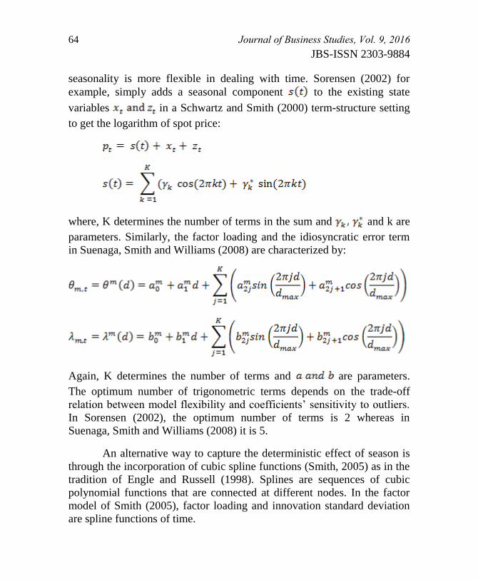
64 Journal of Business Studies, Vol. 9, 2016
JBS-ISSN 2303-9884
seasonality is more flexible in dealing with time. Sorensen (2002) for
example, simply adds a seasonal component to the existing state
variables in a Schwartz and Smith (2000) term-structure setting
to get the logarithm of spot price:
where, K determines the number of terms in the sum and and k are
parameters. Similarly, the factor loading and the idiosyncratic error term
in Suenaga, Smith and Williams (2008) are characterized by:
Again, K determines the number of terms and are parameters.
The optimum number of trigonometric terms depends on the trade-off
relation between model flexibility and coefficients‟ sensitivity to outliers.
In Sorensen (2002), the optimum number of terms is 2 whereas in
Suenaga, Smith and Williams (2008) it is 5.
An alternative way to capture the deterministic effect of season is
through the incorporation of cubic spline functions (Smith, 2005) as in the
tradition of Engle and Russell (1998). Splines are sequences of cubic
polynomial functions that are connected at different nodes. In the factor
model of Smith (2005), factor loading and innovation standard deviation
are spline functions of time.
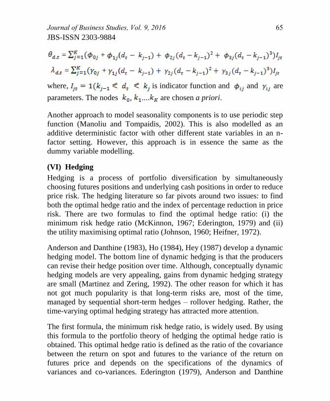
Journal of Business Studies, Vol. 9, 2016 65
JBS-ISSN 2303-9884
= + (
= + (
where, is indicator function and and are
parameters. The nodes , .... are chosen a priori.
Another approach to model seasonality components is to use periodic step
function (Manoliu and Tompaidis, 2002). This is also modelled as an
additive deterministic factor with other different state variables in an n-
factor setting. However, this approach is in essence the same as the
dummy variable modelling.
(VI) Hedging
Hedging is a process of portfolio diversification by simultaneously
choosing futures positions and underlying cash positions in order to reduce
price risk. The hedging literature so far pivots around two issues: to find
both the optimal hedge ratio and the index of percentage reduction in price
risk. There are two formulas to find the optimal hedge ratio: (i) the
minimum risk hedge ratio (McKinnon, 1967; Ederington, 1979) and (ii)
the utility maximising optimal ratio (Johnson, 1960; Heifner, 1972).
Anderson and Danthine (1983), Ho (1984), Hey (1987) develop a dynamic
hedging model. The bottom line of dynamic hedging is that the producers
can revise their hedge position over time. Although, conceptually dynamic
hedging models are very appealing, gains from dynamic hedging strategy
are small (Martinez and Zering, 1992). The other reason for which it has
not got much popularity is that long-term risks are, most of the time,
managed by sequential short-term hedges – rollover hedging. Rather, the
time-varying optimal hedging strategy has attracted more attention.
The first formula, the minimum risk hedge ratio, is widely used. By using
this formula to the portfolio theory of hedging the optimal hedge ratio is
obtained. This optimal hedge ratio is defined as the ratio of the covariance
between the return on spot and futures to the variance of the return on
futures price and depends on the specifications of the dynamics of
variances and co-variances. Ederington (1979), Anderson and Danthine

66 Journal of Business Studies, Vol. 9, 2016
JBS-ISSN 2303-9884
(1981) assume that the covariance matrix between spot and futures return
is always constant which gives a constant optimal hedge ratio. However,
Baillie and Myers (1991) argue that the standard assumption of a time-
invariant optimal hedge ratio is inappropriate. They argue that the
covariance and the variance of spot and futures return depends on the
distribution of prices which changes over time. They define the optimal
hedge ratio by the ratio of conditional covariance between spot and futures
prices to the conditional variance of the futures price. Time variation in
the conditional covariance matrix is modelled using the multivariate
GARCH model. The daily futures price data of six commodities (Beef,
coffee, corn, cotton, gold, soybeans) over two futures contract periods are
used to calculate the optimal hedge ratio via GARCH model. The result
shows that time-invariant optimal hedge ratio is inappropriate.
Moschini and Myers (2002) use multivariate generalized GARCH model
and reject the null hypothesis that optimal hedge ratio is constant. They
also reject that optimal hedge ratio is solely explained by the seasonality
and time to maturity.
The analysis of Suenaga, Smith and Williams (2008) has a profound
implication in determining the optimal hedging strategy under seasonal
and cross-sectional variation in the volatility of futures price. The central
point of their analysis is that the POTS model causes the factor loadings to
have seasonal and cross sectional variations whereas the traditional term-
structure models determine the factor loadings by the time-to-maturity.
Accordingly, the optimal hedge ratio that varies by contract delivery date
can effectively be explained under the POTS framework rather than under
the traditional term-structure model where optimal portfolio depends on
the nearby contract. The hedger‟s decision variable thus reduces to finding
a specific futures contract that can be included in the optimal portfolio.
The contracts whose highest share of price volatility is explained by the
common factor are included in the optimal portfolio. To avoid
idiosyncratic volatility, at least three-month-ahead contracts should be
used. These criteria suggest that for hedging strategy of NYMEX natural
gas the optimal portfolio should include four contracts: „the December
contract‟ for the period of mid May to mid August (September to
November contracts are avoided due to high idiosyncratic variance
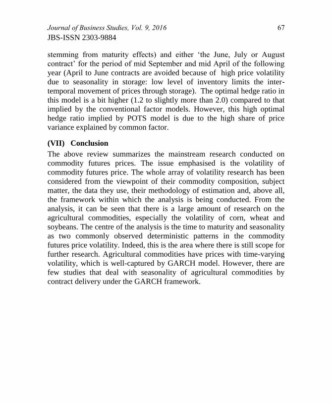
Journal of Business Studies, Vol. 9, 2016 67
JBS-ISSN 2303-9884
stemming from maturity effects) and either „the June, July or August
contract‟ for the period of mid September and mid April of the following
year (April to June contracts are avoided because of high price volatility
due to seasonality in storage: low level of inventory limits the inter-
temporal movement of prices through storage). The optimal hedge ratio in
this model is a bit higher (1.2 to slightly more than 2.0) compared to that
implied by the conventional factor models. However, this high optimal
hedge ratio implied by POTS model is due to the high share of price
variance explained by common factor.
(VII) Conclusion
The above review summarizes the mainstream research conducted on
commodity futures prices. The issue emphasised is the volatility of
commodity futures price. The whole array of volatility research has been
considered from the viewpoint of their commodity composition, subject
matter, the data they use, their methodology of estimation and, above all,
the framework within which the analysis is being conducted. From the
analysis, it can be seen that there is a large amount of research on the
agricultural commodities, especially the volatility of corn, wheat and
soybeans. The centre of the analysis is the time to maturity and seasonality
as two commonly observed deterministic patterns in the commodity
futures price volatility. Indeed, this is the area where there is still scope for
further research. Agricultural commodities have prices with time-varying
volatility, which is well-captured by GARCH model. However, there are
few studies that deal with seasonality of agricultural commodities by
contract delivery under the GARCH framework.
68 Journal of Business Studies, Vol. 9, 2016
JBS-ISSN 2303-9884
References
Anderson, R. W. “Some Determinants of the Volatility of Futures Prices.”
The Journal of Futures Markets, 1985, 5(3), pp. 331-348.
Anderson, T. G. and Bollerslev, T. “Intraday Periodicity and Volatility
Persistence in Financial Markets.” Journal of Empirical Finance,
1997, 4(2-3), pp. 115-158.
Anderson, R. W. and Danthine, J. P. “Cross-Hedging” Journal of Political
Economy, 1981, 89(6), pp. 1182-96.
Anderson, R. W. and Danthine, J. P. “Time and Pattern of Hedging and
the Volatility of Futures Prices” Review of Economic Studies, 1983,
50(2), pp. 249-266.
Baillie, R. and Myers, R. “Bivariate GARCH Estimation of the Optimal
Commodity Futures Hedge.” Journal of Applied Econometrics, 1991,
6(2), pp. 109-124.
Bessembinder, H. “An Empirical Analysis of Risk Premia in Futures
Markets.” The Journal of Futures Markets, 1993, 13(6), pp. 611-30.
Bessembinder, H., Coughenour, J. F., Seguin, P. J. and Smoller, M. M.
“Mean Reversion in Equilibrium Asset Prices: Evidence from the
Futures Term Structure” The Journal of Finance, 1995, 50(1), pp.
361-375.
Black, F. and Scholes, M. “The Pricing of Options and Corporate
Liabilities.” Journal of Political Economy, 1973, 81(3), pp. 637-654.
Blank, S. C. “Research on Futures Markets: Issues, Approaches, and
Empirical Findings.” Western Journal of Agricultural Economics,
1989, 14(1), pp. 126-139.
Brennan, M. J. “The Supply of Storage.” American Economic Review,
1958, 48(1), pp. 50-72.
Brennan, M. J. “The Price of Convenience and the Valuation of Commodity
Contingent Claims.” In Lund, D. and Oksendal, B. (ed), Stochastic Models
and option Values, 1991, vol. 200, Elsevier Science, New York, pp. 33-71.
Brennan, M. J. and Schwartz, E. S. “Evaluating Natural Resource
Investments.” The Journal of Business, 1985, 58(2), pp. 135-157.
Carter, C. A. “Commodity Futures Markets: A Survey.” Australian
Journal of Agricultural and Resource Economics, 1999, 43(2), pp.
209-248.

Journal of Business Studies, Vol. 9, 2016 69
JBS-ISSN 2303-9884
Casassus, J. and Collin-Dufresne, P. “Stochastic Convenience Yield
Implied from Commodity Futures and Interest Rates” The Journal of
Finance, 2005, 60(5), pp. 2283-2331.
Castelino, M.G. “Price Volatility of Futures Contracts: The Maturity
Effects.” Mimeo, Hofstra University, 1982.
Chambers, M. J. and Bailey R. E. “A Theory of Commodity Price
Fluctuations.” Journal of Political Economy, 1996, 104(5), pp. 924-
957.
Chatrath, A., Adrangi, B. and Dhanda, K. K. “Are Commodity Prices
Chaotic?” Agricultural Economics, 2002, 27, pp. 123-137.
Cootner, P.H. “Returns to Speculators: Telser versus Keynes.” Journal of
Political Economy, 1960, 62(4), pp. 396-404.
Cornel, B. “The Relationship between Volume and Price Variability in
Futures Markets.” The
Journal of Futures Markets, 1981, 1(3), pp. 303-316.
Cortazar, G. and Schwartz, E. S. “The Evaluation of Commodity
Contingent Claims.” Journal of Derivatives, 1994, 1(4), pp. 27-39.
Cortazar, G. and Schwartz, E. S. “Implementing a Real Option Model for
Valuing an Undeveloped Oil Field.” International Transactions in
Operational Research, 1997, 4(2), pp. 125-137.
Cortazar, G. and Schwartz, E. S. “Implementing a Stochastic model for
Oil Futures Prices” Energy Economics, 2003, 25(3), pp. 215-238.
Cox, J. C., Ingersoll, Jr. J. E. and Ross, S. A. “The Relation between
Forward Prices and Futures Prices.” Journal of Financial Economics,
1981, 9(4), pp. 321-346.
Deaton, A. and Laroque G. “On the Behaviour of Commodity Prices.”
Review of Economic Studies, 1992, 59(1), pp. 1-23.
Dixit, A. K. and Pindyck, R. S. Investment under Uncertainty, Princeton
University Press, Princeton, New Jersey, 1994.
Dusak K. “Futures Trading and Investor Returns: An Investigation of
Commodity Market Risk Premiums.” Journal of Political Economy,
1973, 81(6), pp. 1387-1406.
Ederington, L. H. “The Hedging Performance of the New Futures
Markets.” The Journal of Finance, 1979, 34(1), pp. 157-170.
70 Journal of Business Studies, Vol. 9, 2016
JBS-ISSN 2303-9884
Engle, R. F. and Russell, J. R. “Autoregressive Conditional Duration: A
New Model for Irregularly Spaced Transaction Data.” Econometrica,
1998, 66(5), pp. 1127-1162.
Fama, E. F. and French K. R. “Commodity Futures Prices: Some Evidence
on Forecast Power, Premiums, and the Theory of Storage.” Journal of
Business, 1987, 60(1), pp. 55-73.
Gabillon, J. “The Term Structure of Oil Futures Prices”, Working Paper,
Oxford Institute of Energy Studies, 1992.
Garcia, P. and Leuthold, R. M. “A Selected Review of Agricultural
Commodity Futures and Options Markets.” European Review of
Agricultural Economics, 2004, 31(3), pp. 235-272.
Gibson, R. and Schwartz, E. S. “Stochastic Convenience Yield and the
Pricing of Oil Contingent Claims.” The Journal of Finance, 1990,
45(3), pp. 959-976.
Goodwin, B. K. and Schnepf, R. “Determinants of Endogenous Price Risk
in Corn and Wheat Futures Markets.” The Journal of Futures
Markets, 2000, 20(8), pp. 753-774.
Gray, R. W. and Rutledge, D.J.S. “The Economics of Commodity Futures
Market: A Survey.” Review of Marketing and Agricultural
Economics, 1971, 39(4), pp. 57-108.
Gustafson, R. L. “Carryover Levels for Grains.” in US Department of
Agriculture Technical Bulletin 1178, 1958.
Hannan, E. J., Terrel, R. D. and Tuckwell, N. “The Seasonal Adjustment
of Economic Time Series.” International Economic Review, 1970, 11(1),
pp. 24-52.
Heath, D., Jarrow, A. and Morton, A. J. “Bond Pricing and the Term
Structure of Interest Rates: A New Methodology for Contingent
Claims Valuation.” Econometrica, 1992, 60(1), pp. 77-105.
Heifner, R. G. “Optimal Hedging Levels and Hedging Effectiveness in
Cattle Feeding.” Agricultural Economics Research, 1972, 24(2), pp.
25-36.
Hennessy, D. A. and Wahl, T. I. “The Effects of Decision Making on
Futures Price Volatility.” American Journal of Agricultural
Economics, 1996, 78(3), pp. 591-603.

Journal of Business Studies, Vol. 9, 2016 71
JBS-ISSN 2303-9884
Hey, J. D. “The Dynamic Competitive Firm under Spot Price
Uncertainty.” Manchester School of Economics and Social Studies,
1987, 55(1), pp. 1-12.
Hicks, J. R. Value and Capital, Clarendon Press, Oxford, 1946.
Hilliard, J. E. and Reis, J. “Valuation of Commodity Futures and Options
under Stochastic Convenience Yields, Interest Rates, and Jump
Diffusions in the Spot.” Journal of Financial and Quantitative
Analysis, 1998, 33(1), pp. 61-86.
Ho, T. “Inter-temporal Commodity Futures Hedging and the Production
Decision” The Journal of Finance, 1984, 3(2), pp. 351-376.
Johnson, L. “The Theory of Hedging and Speculation in Commodity
Futures.” The Review of Economic Studies, 1960, 27(3), pp. 139-51.
Kaldor, N. “A Note on the Theory of Forward Market.” The Review of
Economic Studies, 1940, 7(3), pp. 196- 201.
Kalev, P. S. and Duong H. N. “A Test of the Samuelson Hypothesis Using
Realized Range.” The Journal of Futures Markets, 2008, 28(7), pp.
680-696.
Kamara, A. “Issues in Futures Markets: A Survey.” The Journal of
Futures Markets, 1982, 2(3), pp. 261-294.
Karali, B., Dorfman, J. H. and Thurman, W. N. “Delivery Horizon and
Grain Market Volatility.” The
Journal of Futures Markets, 2010, 30(9), pp. 846-873.
Karali, B., Dorfman, J. H. and Thurman, W. N. “Do Volatility
Determinants Vary across Futures Contracts? Insights from a
Smoothed Bayesian Estimator.” The Journal of Futures Markets,
2010, 30(3), pp. 257-277.
Karali, B. and Thurman, W. N. “Announcement Effects and the Theory of
Storage: An Empirical Study of Lumber Futures.” Agricultural
Economics, 2009, 40(4), pp. 421-436.
Karali, B. and Thurman, W. N. “Components of Grain Futures Price
Volatility” Journal of Agricultural and Resource Economics, 2010,
35(2), pp. 167-182.
Kenyon, D., Kling, K., Jordan, J., Seale, W. and McCabe, N. “Factors
Affecting Agricultural Futures Price Variance.” The Journal of
Futures Markets, 1987, 7(1), pp. 73-91.

72 Journal of Business Studies, Vol. 9, 2016
JBS-ISSN 2303-9884
Keynes, J. M. “Some Aspects of Commodity Markets” Manchester
Guardian Commercial, European Reconstruction Series, 1923,
Section 13, pp. 784-86.
Khoury, N. and Yourougou P. “Determinants of Agricultural Futures Price
Volatilities: Evidence from Winnipeg Commodity Exchange.” The
Journal of Futures Markets, 1993, 13(4), pp. 345-356.
Kolb, R.W. “Is Normal Backwardation Normal?” The Journal of Futures
Markets, 1992, 12(1), pp. 75-91.
Kyle, A. S. “Continuous Auctions and Insider Trading.” Econometrica,
1985, 53(6), pp. 1315-1335.
Lautier, D. “Term Structure Models of Commodity Prices.” The Journal
of Alternative Investment, 2005, 8(1), pp. 42-64.
Manoliu, M. and Tompaidis, S. “Energy Futures Prices: Term Structure
Models with Kalman Filter Estimation.” Applied Mathematical
Finance, 2002, 9(1), pp. 21-43.
Martinez, S. W. and Zering, K. D. “Optimal Dynamic Hedging Decisions
for Grain Producers”, American Journal of Agricultural Economics,
1992, 74(4), pp. 879-88.
McKenzie, A. M., Jiang, B., Djunaidi, H., Hoffman, L. A. and Wailes, E.
J. “Unbiasedness and Market Efficiency Tests of the US Rice Futures
Markets.” Review of Agricultural Economics, 2002, 24(2), pp. 474-
493.
McKinnon, R.I. “Futures Markets, Buffer Stocks and Income Stability for
Primary Producers.” Journal of Political Economy, 1967, 75(6), pp.
844-61.
Miller, K. D. “The Relation between Volatility and Maturity in Futures
Contracts,” in R.M. Leuthold, (Ed.) Commodity Markets and Futures
Prices Chicago Mercantile Exchange, Chicago, IL, 1979.
Milliaris, A. G. “Futures Markets. 3 Vols.” Elgar Reference Collection
International Library of Critical Writings in Financial Economics
Cheltenham and Lyme (ed), NH: Elgar, 1997.
Milonas, M. “Price Variability and the Maturity Effect.” The Journal of
Futures Market, 1986, 6(3), pp. 443-460.
Moschini, G. and Myers, R. J. “Testing for Constant Hedge Ratios in
Commodity Markets: A Multivariate GARCH Approach.” Journal of
Empirical Finance, 2002, 9(5), pp. 589-603.
Journal of Business Studies, Vol. 9, 2016 73
JBS-ISSN 2303-9884
Muth, J. F. “Rational Expectations and the Theory of Price Movements.”
Econometrica, 1961, 29(3), pp. 315-335.
Ng, V. K. and Pirrong, S. C. “Fundamentals and Volatility: Storage,
Spreads, and the Dynamics of Metals Prices.” Journal of Business,
1994, 67(2), pp. 203-230.
Ovararin, K. and Meade, N. “Mean Reversion and Seasonality in GARCH
of Agricultural Commodities.” International Conference on Applied
Economics (ICOAE), 2010.
Poon, S. and Granger, C. “Practical Issues in Forecasting Volatility.”
Financial Analysts Journal, 2005, 61(1), pp. 45-56.
Richter, M. and Sørensen, C. “Stochastic Volatility and Seasonality in
Commodity Futures and Options: The Case of Soybeans” Working
Paper, Department of Finance, Copenhagen Business School,
Copenhagen, Denmark, 2002.
Rutledge, D. J. S. “A Note on the Variability of Futures Prices.” The
Review of Economics and Statistics, 1976, 58(1), pp. 118-120.
Samuelson, P. A. “Proof that Properly Anticipated Prices Fluctuate
Randomly.” Industrial Management Review, 1965, 6(2), pp. 41-49.
Schaefer, M. P., Myers, R. J. and Koontz, S. R. “Rational Expectations
and Market Efficiency in the US Live Cattle Futures Market: The
Role of Proprietary Information.” The Journal of Futures Markets,
2004, 24(5), pp. 429-451.
Schwartz, E.S. “The Stochastic Behaviour of Commodity Prices:
Implications for Valuation and Hedging.” The Journal of Finance,
1997, 52(3), pp. 923-973.
Schwartz, E. S. and Smith, J. E. “Short-Term Variations and Long-Term
Dynamics in Commodity Prices.” Management Science, 2000, 46(7),
pp. 893-911.
Sorensen, C. “Modelling Seasonality in Agricultural Commodity Futures.”
The Journal of Futures Markets, 2002, 22(5), pp. 393-426.
Smith, A. “Partially Overlapping Time Series: A New Model for Volatility
Dynamics in Commodity Futures.” Journal of Applied Econometrics,
2005, 20(3), pp. 405-422.
Stein, J. L. “Spot, Forward and Futures.” Research in Finance, 1979, 1,
pp. 225-310.
74 Journal of Business Studies, Vol. 9, 2016
JBS-ISSN 2303-9884
Streeter, D. H. and Tomek, W. G. “Variability in Soybean Futures Prices:
An Integrated Framework.” The Journal of Futures Markets, 1992,
12(6), pp. 705-728.
Suenaga, H. and Smith, A. “Volatility Dynamics and Seasonality in
Energy Prices: Implications for Crack-Spread Price Risk.” The
Energy Journal, 2011, 32(3), pp. 27-58.
Suenaga, H., Smith A. and Williams J. “Volatility Dynamics of NYMEX
Natural Gas Futures Prices.” The Journal of Futures Markets, 2008,
28(5), pp. 438-463.
Telser, L. G. “Futures Trading and the Storage of Cotton and Wheat.”
Journal of Political Economy, 1958, 57(3), pp. 233-55.
Todorova, M. I. “Modelling Energy Commodity Futures: Is Seasonality
Part of It?” Journal of Alternative Investment, 2004, 7(2), pp. 10-32.
Vasicek, O. “An Equilibrium Charaterization of the Term Structure”.
Journal of Financial Economics, 1977, 5(2), pp. 177-188.
Williams, J. C. The Economic Function of Futures Markets, Cambridge:
Cambridge University Press, 1989.
Williams, J. C. and Wright, B. D. Storage and Commodity Markets,
Cambridge University Press, New York, 1991.
Wright, B. D. and Williams, J. C. “The Economic Role of Commodity
Storage.” Economic Journal, 1982, 92, pp. 596-614.
Working, H. “Theory of the Inverse Carrying Charge in Futures Markets.”
Journal of Farm Economics, 1948, 30(1), pp. 1-28.
Working, H. “The Theory of Price of Storage.” The American Economic
Review, 1949, 39(6), pp.1254-1262.
Yang, S. R. and Brorsen, B. W. “Non-linear Dynamics of Daily Futures
Prices: Conditional Heteroskedasticity or Chaos?” The Journal of
Futures Markets, 1993, 13(2), pp. 175-191.
Journal of Business Studies, Vol. 9, 2016 75
JBS-ISSN 2303-9884
Impact of Market Size and Foreign Trade on FDI Inflow in
Bangladesh: A VEC Approach
Rakibul Islam
Abstract
This study investigated the effect of market size and foreign trading on FDI
inflow in Bangladesh over the period of 1986 to 2012 by using a vector error
correction model. The long term co-integration result identified the positive
impact of GDP and Export on FDI inflow and negative impact of Import on FDI.
Besides significant F value of VECM estimates suggest the overall short run
relationship among the variable under study. In short run, two year lagged export
and one year lagged import has positive impact on FDI inflow in Bangladesh.
The VEC granger causality result revealed strong unidirectional relation of
Export and Import to FDI inflow, FDI inflow to GDP, Import to Export and a
mild unidirectional relation of FDI to Import.
Keywords: Foreign direct investment, co-integration, gross domestic product,
export, import
(I) Introduction
he immense contribution of inflow of Foreign Direct Investment
(FDI) proved to be significant in many theoretical and empirical
researches conducted in many countries at different times by identifying
the improvement of host countries‘ infrastructural, technological,
entrepreneurial, social and financial resources (Adams 2009, Bergten, et
al. 1978, Seid 2002, Romer 1986, 1994, Lucas 1988, Mankiw et al. 1992,
Pugel 2007, Grossman and Helpman 1991, Nair–Reichert and Weinhold
2001). In addition, the study of United Nation Conference on Trade and
Development (UNCTAD) in 1992 also examine the truth of FDI led
growth hypothesis in developing economies and advocate initiatives to
encourage FDI to flourish economic growth in developing nations (Agosin
and Mayer 2000).
Lecturer, Department of Banking and Insurance, University of Rajshahi,
E-mail: [email protected]
T
76 Journal of Business Studies, Vol. 9, 2016
JBS-ISSN 2303-9884
Bangladesh thriving for rapid growth with huge prospect should look
forward to expand FDI inflow to accelerate the momentum. The influence
of market size of a country and its level of foreign trading on FDI inflow
pronounced in different literatures (Charkrabarti 2001, Jordaan 2004)
induces the study conducted for Bangladesh with a more advanced
methodology for exploration and explanation of nexus as well as
anomalies of FDI inflow. Market size hypothesis of FDI predicts the flow
of FDI to the nations with larger market having greater ability to exploit
resources to derive economic of scale. Whereas, level of foreign trading
effect to FDI decision according to the nature and purpose of FDI. Unlike
export base FDI attracted by Open Export Policy, market seeking FDI
moves to that location where import barrier exists (Jordaan 2004). As a
result, the study used export and import separately to identify impact of
foreign trade on FDI inflow in Bangladesh.
The study set to identify the long-run equilibrium relationship between
GDP, Export, Import and FDI inflow and short run causal direction to
evaluate the impact of market size and foreign trading on FDI inflow in
Bangladesh. The remainder of the paper proceeds with Section II
exploring the brief review of empirical literature, Section III explains
theoretical framework of the study, Section IV shows the methodology;
Section V presents empirical results and Section VI draws conclusion.
(II) Brief Review of Empirical Literature
There are different perplexing results found after observing the empirical
literature supporting different theories for FDI. One major thing observed
that FDI and GDP have positive bidirectional relationship (Hsiao and Shen
2003) contrasting the negative on average relationship found by
Mencinger (2003) while Arshad and Muhammad (2012) signifies no
relation between them. It has been found that there are bidirectional
causality between FDI and trade (export and import) in case of developing
countries (Aizenmana and Noy, 2006; Fontagne and Pajot, 2000)
contrasting the unidirectional relationships among the variable found by
others (Pantulu and poon 2002). Again one way relationship observed
between FDI and exports has been found by studies (Pantulu and poon,
2002; Srivastava and sen, 2004) while the bidirectional causation between
Journal of Business Studies, Vol. 9, 2016 77
JBS-ISSN 2303-9884
FDI and exports found in developed world (Iqbal et al., 2010). Again, Liu
et al.(2001) reported the existence of unidirectional relationship between
FDI and Exports; Imports and FDI in China. The Following specific
literatures have been presented in brief;
Arshad and Muhammad (2012) analyzed FDI, Investment, Trade (import
and export), Economic growth of Pakistan from 1965 to 2005 by using co-
integrating VAR technique and found long term relationship explaining
import and export effect on GDP but FDI insignificantly affecting GDP
while another long term relationship identifying import and export effect
on FDI but GDP fail to have significant effect on FDI. Therefore they
conclude that FDI and GDP have no significant relation in long run.
Nguyen (2011) used export, import, economic growth data of Malaysia
and Korea from 1970 to 2004 and vector auto regression model had been
employed to explain that all four variables have two way causalities
between each pair except GDP to export in Malaysia, whereas substantial
one way causality from export, import, GDP to FDI, from export and
import to GDP and from export to import observed in Korea.
Sharma and Kaur (2013) examined FDI, trade (export and import) of India
and China from 1976 to 2011 and their Granger- causality result found
that unidirectional causality from FDI to import, FDI to Export and two-
way causality between import and export in China while in case of India
all three variables have bidirectional causality between one another.
Martinez-Martin (2010) test VECM by using annual data from 1993 to
2008 for Spain. They used FDI, export, domestic income, world income
and competitiveness as variables to identify causal relationship among
them. The VECM result found a positive long run relationship exists from
FDI to export.
Mortaza and Narayan (2007) examined FDI inflows, import and export
over GDP, literacy rate and domestic investment and inflation to identify
causal relationship of growth trade liberation and FDI in Bangladesh,
India, Pakistan, Srilanka and Nepal. By employing VAR, panel fixed and
random effect model, they identified unidirectional causality between FDI,
Trade liberation and economic growth for Bangladesh and Pakistan.
78 Journal of Business Studies, Vol. 9, 2016
JBS-ISSN 2303-9884
(III) Theoretical Framework
The paper attempts to trace the long-run and short run equilibrium
relationship between FDI, market size, foreign trading of Bangladesh over
the period of 1986–2012 using the time series framework. In doing so, the
study measures FDI as FDI inflow, Market size as GDP at current USD,
Foreign trading in terms of export as export of goods and services at
current USD and foreign trading in terms of import as import of goods and
services at current USD. All data have been collected from data base of
the World Development Indicators (WDI) and central bank of Bangladesh
(Bangladesh Bank).The sample covers twenty seven annual observations
and all the data converted into natural logarithm to minimize the effect of
heteroskedasticity and multicollinearity among the variable.
The empirical estimation proceeds with the checking of the normality of
the distribution by using Jarque-Bera test. Next, it goes to identify the
existence of unit root under a univariate analysis by employing both
Augmented Dickey-Fuller (ADF) and the Phillips-Perron (PP) tests. The
unit root test has to be conducted at the intercept as well as intercept plus
trend regression form. If the study shows unit root that is data distribution
are non-stationary then they shouldn‘t be used in levels rather their first
differences to identify the level of stationary since in time series data two
or more non-stationary data can be stationary if they are integrated at same
order ie. Order I(1).
If it confirms the stationary of the variables at their differences, the study
then proceeds to draw co-integration relationship between variables by
applying the Johansen-Juselius procedure to identify the long run
relationship among the variables. The notable thing is that to run Johansen
co-integration test, all series must have same order of integration, either in
level or in differenced form. That means the difference between two or
more non-stationary series becomes stationary when they move together in
long-run, while they might float separately in short run.
Though the existence of co-integrating relation identifies long run
equilibrium relationships between variables and existence of at least one
causal relationship among variables, it cannot identify the direction of
causal relationship rather it may produce spurious correlation between
Journal of Business Studies, Vol. 9, 2016 79
JBS-ISSN 2303-9884
variables. Therefore Vector error correction model (VECM) has
employed, over Vector autoregressive model unable to have error
correction term, to identify direction and sources of causal relationship
and distinguish short run and long run relationship for the variables.
(IV) Methodology
Descriptive statistics
The mean, median, mode of the variables are to be defined in descriptive
statistics with the maximum and minimum level and standard deviation to
have an overall condition of the each of the variable within the time frame
analyzed. Whether the data under each variable are normally distributed or
not is the pre- requisite for further analysis.
Unit Root Test
In order to test for short run dynamics and long run relationship among
time series variables, the time series variables are estimated to identify
stationarity of the series by the unit autoregressive tests. In this paper two
methods are used for detecting a unit autoregressive root: (i) The
Augmented Dickey-Fuller (ADF) Test (Dickey and Fuller 1981) and the
Phillips–Perron (PP) Test (Phillips and Perron 1988).
Augmented Dickey-Fuller Test
The ADF test for a unit autoregressive root tests the null hypothesis H0: δ
= 0 against the alternative H1: δ < 0 in the following regression:
(1)
Where Δ is the first difference operator and ut is a white noise error term
and ρ is the number of lags in the dependent variable. In the hypothesis
testing H0statistic is obtained from the OLS t-statistics testing δ = 0 in
equation (1).
If Yt is stationary around a deterministic linear time trend line, then the
trend‗t‘ i.e., the no. of observation should be added as an explanatory
variable. Alternatively (1) can be written as

80 Journal of Business Studies, Vol. 9, 2016
JBS-ISSN 2303-9884
(2)
In the equation (6) Ytis a random walk with drift around a stochastic trend.
Here α2
is an unknown coefficient and the ADF statistic is the OLS t-
statistic testing δ = 0 in (2).
The Phillips–Perron (PP) Test
The results are also verified by Phillips and Perron (1988) test. The test
regression for the PP tests is:
(3)
Where, may be 0, μ, or μ+ βt
and εt
is I(0) and may not be
homoskedastic. Any serial correlation and heteroskedasticity in the error
term εtrectified by the PP tests by a straight modification in the test
statistics tπ= 0 and . The hypothesis testing procedure is the same
asymptotic distributions as the ADF test.
The null hypothesis of a unit root implies that the coefficient of X t−1is zero
i.e., = 0. Series is stationary if null hypothesis is rejected and no
differencing in the series is necessary to induce stationarity. The number
of lags in the dependent variable is chosen by the Akaike Information
Criterion (AIC). Unit root test identifies whether the variables are
stationary or non-stationary. The test is applied on both the original series
(in logarithmic form) and to the first differences. In addition, both models
with and without trend are tried.
Co-integration Test
To identify whether a long run equilibrium relationship exists among time
series variables, Johansen (1988) maximum likelihood approach is readily
used.
The time series variables of FDI function of Bangladesh are considered to
pursue the first order Vector Auto Regressive (VAR) representation
defined as:
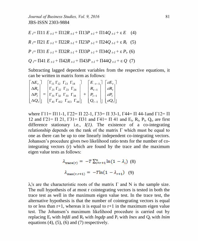
Journal of Business Studies, Vol. 9, 2016 81
JBS-ISSN 2303-9884
E t= Π11 E t-1 + Π12R t-1 + Π13P t-1 + Π14Q t-1 + ε E (4)
R t= Π21 E t-1 + Π22R t-1 + Π23P t-1 + Π24Q t-1 + ε Rt (5)
P t= Π31 E t-1 + Π32R t-1 + Π33P t-1 + Π34Q t-1 + ε Pt. (6)
Q t= Π41 E t-1 + Π42R t-1 + Π43P t-1 + Π44Q t-1 + ε Q (7)
Subtracting lagged dependent variables from the respective equations, it
can be written in matrix form as follows:
t
t
t
t
Q
P
R
E
=
4441341241
34333231
24232221
14131211
+
1
1
1
1
t
t
t
t
Q
P
R
E
t
t
t
t
Q
P
R
E
where Γ11= Π11-1, Γ22= Π 22-1, Γ33= Π 33-1, Γ44= Π 44-1and Γ12= Π
12 and Γ21= Π 21, Γ31= Π31 and Γ41= Π 41 and Et, Rt, Pt, Qt, are first
difference stationary i.e., I(1). The existence of a co-integrating
relationship depends on the rank of the matrix Γ which must be equal to
one as there can be up to one linearly independent co-integrating vectors.
Johansen‘s procedure gives two likelihood ratio tests for the number of co-
integrating vectors (r) which are found by the trace and the maximum
eigen value tests as follows:
(8)
(9)
λi's are the characteristic roots of the matrix Γ and N is the sample size.
The null hypothesis of at most r cointegrating vectors is tested in both the
trace test as well in the maximum eigen value test. In the trace test, the
alternative hypothesis is that the number of cointegrating vectors is equal
to or less than r+1, whereas it is equal to r+1 in the maximum eigen value
test. The Johansen‘s maximum likelihood procedure is carried out by
replacing Et with lnfdi and Rt with lngdp and Pt with lnex and Qt with lnim
equations (4), (5), (6) and (7) respectively.
82 Journal of Business Studies, Vol. 9, 2016
JBS-ISSN 2303-9884
Vector Error Correction Model
The co-integration among variables exclusively illustrates a long run
equilibrium association. However, there may be short run disequilibrium
among them. Vector Error Correction Model (VECM) can be developed to
explore the short run dynamics among the concerned time series variables.
Therefore, an unrestricted VECM (Granger 1988) taking into account up
to ρ lags for FDI.
(10)
Particularly, in this model, the parameter (λ) of the lagged error correction
term (et−1) exhibits the long-run association in time series variables under
study, and also the speed of correction from the short-run to the long-run
equilibrium situation. The lag-length of the variables has been
appropriated through final prediction error (FPE) criterion (H.Akaike
1969) to surmount the under or over parameterization problem which may
provoke in efficiency and bias in the estimates. Remarkably, the parameter
of the error correction term should be negative and statistically significant
in terms of its associated t value to confirm the long-run equilibrium
relationship in the variables. The variation in GDP, Export, and Import
cause the variation in FDI when bi‘s, ci‘s, di‘s are significant in terms of
the F test (Bahmani and Payesteh 1993). The stability of the VEC model
has examined by the inverse roots of the AR characteristic polynomial test
as well as cusum and cusumq.
(V) Empirical Results and Discussion
Descriptive Statistics
The descriptive statistics of the variables under study have been presented
in Table I. The Jarque-Bera test statistics fails to reject the null hypothesis
of normal distribution of each variable, which substantiates the normality
of the series. Besides, the numeric of kurtosis for each variable is found
below 2.5, which indicates the normality of distribution. The figure for
skewness of each variable is found to be mild and negative skewed, except
for the GDP and Import, those have slight positive skewness. The standard
deviation of the series is low compared to mean, which point out a small
coefficient of variation except for FDI inflow. In addition, the range of
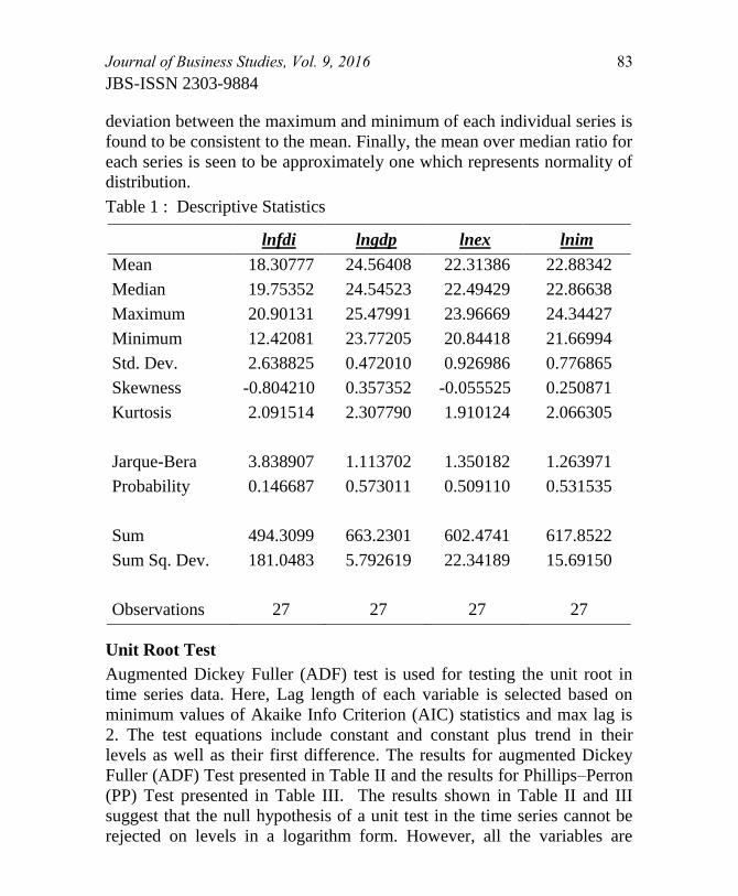
Journal of Business Studies, Vol. 9, 2016 83
JBS-ISSN 2303-9884
deviation between the maximum and minimum of each individual series is
found to be consistent to the mean. Finally, the mean over median ratio for
each series is seen to be approximately one which represents normality of
distribution.
Table 1 : Descriptive Statistics
lnfdi lngdp lnex lnim
Mean 18.30777 24.56408 22.31386 22.88342
Median 19.75352 24.54523 22.49429 22.86638
Maximum 20.90131 25.47991 23.96669 24.34427
Minimum 12.42081 23.77205 20.84418 21.66994
Std. Dev. 2.638825 0.472010 0.926986 0.776865
Skewness -0.804210 0.357352 -0.055525 0.250871
Kurtosis 2.091514 2.307790 1.910124 2.066305
Jarque-Bera 3.838907 1.113702 1.350182 1.263971
Probability 0.146687 0.573011 0.509110 0.531535
Sum 494.3099 663.2301 602.4741 617.8522
Sum Sq. Dev. 181.0483 5.792619 22.34189 15.69150
Observations 27 27 27 27
Unit Root Test
Augmented Dickey Fuller (ADF) test is used for testing the unit root in
time series data. Here, Lag length of each variable is selected based on
minimum values of Akaike Info Criterion (AIC) statistics and max lag is
2. The test equations include constant and constant plus trend in their
levels as well as their first difference. The results for augmented Dickey
Fuller (ADF) Test presented in Table II and the results for Phillips–Perron
(PP) Test presented in Table III. The results shown in Table II and III
suggest that the null hypothesis of a unit test in the time series cannot be
rejected on levels in a logarithm form. However, all the variables are
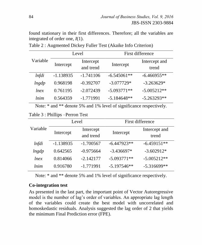
84 Journal of Business Studies, Vol. 9, 2016
JBS-ISSN 2303-9884
found stationary in their first differences. Therefore; all the variables are
integrated of order one, I(1).
Table 2 : Augmented Dickey Fuller Test (Akaike Info Criterion)
Variable
Level First difference
Intercept Intercept
and trend Intercept
Intercept and
trend
lnfdi -1.138935 -1.741106 -6.545061** -6.466955**
lngdp 0.968198 -0.392707 -3.077729* -3.263629*
lnex 0.761195 -2.072439 -5.093771** -5.005212**
lnim 0.564359 -1.771991 -5.184648** -5.263293**
Note: * and ** denote 5% and 1% level of significance respectively.
Table 3 : Phillips –Perron Test
Variable
Level First difference
Intercept Intercept
and trend Intercept
Intercept and
trend
lnfdi -1.138935 -1.700567 -6.447923** -6.459151**
lngdp 0.642565 -0.975664 -3.436697* -3.602912*
lnex 0.814066 -2.142177 -5.093771** -5.005212**
lnim 0.916780 -1.771991 -5.197546** -5.316699**
Note: * and ** denote 5% and 1% level of significance respectively.
Co-integration test
As presented in the last part, the important point of Vector Autoregressive
model is the number of lag‘s order of variables. An appropriate lag length
of the variables could create the best model with uncorrelated and
homoskedastic residuals. Analysis suggested the lag order of 2 that yields
the minimum Final Prediction error (FPE).
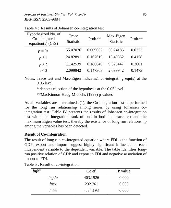
Journal of Business Studies, Vol. 9, 2016 85
JBS-ISSN 2303-9884
Table 4 : Results of Johansen co-integration test
Hypothesized No. of
Co-integrated
equation(s) (CEs)
Trace
Statistic Prob.**
Max-Eigen
Statistic Prob.**
55.07076 0.009062 30.24185 0.0223
24.82891 0.167619 13.40352 0.4158
11.42539 0.186649 9.325447 0.2601
r ≤ 3 2.099942 0.147303 2.099942 0.1473
Notes: Trace test and Max-Eigen indicates1 co-integrating eqn(s) at the
0.05 level
* denotes rejection of the hypothesis at the 0.05 level
**MacKinnon-Haug-Michelis (1999) p-values
As all variables are determined I(1), the Co-integration test is performed
for the long run relationship among series by using Johansen co-
integration test. Table IV presents the results of Johansen co-integration
test with a co-integration rank of one in both the trace test and the
maximum Eigen value test; thereby the existence of long run relationship
among the variables has been detected.
Result of Co-integration
The result of long run co-integrated equation where FDI is the function of
GDP, export and import suggest highly significant influence of each
independent variable to the dependent variable. The table identifies long-
run positive relation of GDP and export to FDI and negative association of
import to FDI.
Table 5 : Result of co-integration
lnfdi Co.ef. P value
lngdp 403.1926 0.000
lnex 232.761 0.000
lnim -534.193 0.000

86 Journal of Business Studies, Vol. 9, 2016
JBS-ISSN 2303-9884
Vector Error Corrected results
The following Table VI postulates the outcome of the vector error
correction model. To initiate VEC model, the appropriate lag length (lag
02) has been selected by FPE criterion (H. Akaike 1969). The table reveals
the long run equilibrium relationship justified among variables as
estimated parameter (λ) of the error correction term (et−1) is negative and
statistically significant at 1 percent level of significance., implies a long
run causality as well as long run convergence with (-0.0264). Followed by
that result, table VI presents the short run components of estimated vector
error corrected model (VECM). The existence of overall short run
variation found significant as F statistics is 2.558. The result of R square
showed that the short run variation of GDP, Export, and Import explains
37.88 percent variation of FDI on average.
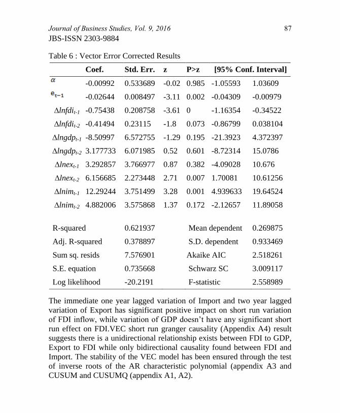
Journal of Business Studies, Vol. 9, 2016 87
JBS-ISSN 2303-9884
Table 6 : Vector Error Corrected Results
Coef. Std. Err. z P>z [95% Conf. Interval]
-0.00992 0.533689 -0.02 0.985 -1.05593 1.03609
-0.02644 0.008497 -3.11 0.002 -0.04309 -0.00979
∆lnfdit-1 -0.75438 0.208758 -3.61 0 -1.16354 -0.34522
∆lnfdit-2 -0.41494 0.23115 -1.8 0.073 -0.86799 0.038104
∆lngdpt-1 -8.50997 6.572755 -1.29 0.195 -21.3923 4.372397
∆lngdpt-2 3.177733 6.071985 0.52 0.601 -8.72314 15.0786
∆lnext-1 3.292857 3.766977 0.87 0.382 -4.09028 10.676
∆lnext-2 6.156685 2.273448 2.71 0.007 1.70081 10.61256
∆lnimt-1 12.29244 3.751499 3.28 0.001 4.939633 19.64524
∆lnimt-2 4.882006 3.575868 1.37 0.172 -2.12657 11.89058
R-squared 0.621937 Mean dependent 0.269875
Adj. R-squared 0.378897 S.D. dependent 0.933469
Sum sq. resids 7.576901 Akaike AIC 2.518261
S.E. equation 0.735668 Schwarz SC 3.009117
Log likelihood -20.2191 F-statistic 2.558989
The immediate one year lagged variation of Import and two year lagged
variation of Export has significant positive impact on short run variation
of FDI inflow, while variation of GDP doesn‘t have any significant short
run effect on FDI.VEC short run granger causality (Appendix A4) result
suggests there is a unidirectional relationship exists between FDI to GDP,
Export to FDI while only bidirectional causality found between FDI and
Import. The stability of the VEC model has been ensured through the test
of inverse roots of the AR characteristic polynomial (appendix A3 and
CUSUM and CUSUMQ (appendix A1, A2).
88 Journal of Business Studies, Vol. 9, 2016
JBS-ISSN 2303-9884
(VI) Conclusion
This study investigated the effect of market size and foreign trading on
FDI inflow in Bangladesh over the period of 1986 to 2012 by using a
vector error correction model. The results of ADF and PP unit root test
identified that all variables in the study were integrated in order one I(1).
The test statistics (trace and max-eigen) of the Johansen co-integration test
have been conducted on intercept without trend regression identified the
presence of a co-integrated relationship among the variables. Again, the
negative parameter of error correction term validates the existence of long
run equilibrium relationship among the variables with a highly significant
t value. The long term co-integration result identified the positive impact
of GDP and Export on FDI inflow and negative impact Import on FDI.
Besides significant F-value of VECM estimates suggest the overall short
run relationship among the variable under study. In short run, two year
lagged export and one year lagged import have positive impact on FDI
inflow in Bangladesh. The VEC granger causality result showed strong
unidirectional relation of Export and Import to FDI inflow, FDI inflow to
GDP, Import to Export and a mild unidirectional relation of FDI to Import.
Therefore, the VEC model identified a long run equilibrium association in
the variables and short run causal flow between them.
The policy implication of this study can be abridged under following
points. Firstly, the Govt. of Bangladesh should exploit these macro-
economic variables carefully on a long run basis to reap the benefit from
their nexus. Secondly, the positive relation of GDP, Export and FDI
provides the Govt. with information that the growth in GDP and Export
can substantially raise FDI inflow and FDI will in turn accelerate Export
and GDP. Therefore, FDI driven growth and growth led FDI policy should
be advocated simultaneously. In addition, the long run negative
association between FDI and Import should be viewed as import
substituting policy for the country, so that current account deficit can be
lessened in the long run. Thirdly, in short run perspective, Export and
Import have great influence on FDI. The contrasting feature found in
short run case Import has positive relation to FDI against long run can be
rationalized by substantial capital goods import requirement to initiate FDI
that is to establish plants and operations in Bangladesh. Govt. should

Journal of Business Studies, Vol. 9, 2016 89
JBS-ISSN 2303-9884
provide special facilities and provision for capital goods import to
accelerate FDI inflow in short run, causing decrease of aggregate import
by producing goods and services to meet the domestic needs and rise in
export to meet the international demand. Furthermore, the long run
positive relation between FDI inflow and GDP hasn‘t been pronounced in
the short run, because FDI follows long run performance of GDP of a
country while factors initiating FDI inflow remains the foreign trading in
Bangladesh. In nutshell, a comprehensive but target oriented sector basis
short run export and import policies focusing long term benefit out of it
should be managed and practiced effectively.
References
Adams, S. 2009. ―Foreign Direct Investment, Domestic Investment, and
Economic Growth in Sub- Saharan Africa.‖ Journal of Policy
Modeling, 31:939-949.
Agosin, M.R., & Mayer, R. 2000. ―Foreign Investment in Developing
Countries: Does It Crowd in Domestic Investment?‖ UNCTAD
Discussion Paper 146, Geneva, Switzerland.
Aizenmana and Noy, 2006. ―FDI and Trade—Two-Way Linkages?‖, The
Quarterly Review of Economics and Finance, 46(3): 317–337.
Akinlo, A.E. 2003. ―Foreign Direct Investment and Economic Growth In
sub-Saharan Africa.‖ International Review of Economics and
Business 50: 569-580
Aluko, S.A. 1961. ―Financing Economic Development in Nigeria‖. The
Nigerian Journal of Economic and Social Studies, 3(1): 39–67.
Amin, S. 1974. ―Accumulation on a World Scale: A Critique of the
Theory of Underdevelopment”. New York, Monthly Review Press.
Arshad, Muhammad. 2012. ―Impact of Foreign Direct Investment on
Trade and Economic Growth of Pakistan: A Co-integration
Analysis.‖,Int. J. Eco. Res, 3(4): 42-75.
Bahmani-Oskooee M. and Payesteh S. 1993. ―Budget Deficits and The
Value of The Dollar: An Application of Cointegration and Error-
Correction Modeling,‖ Journal of Macroeconomics, 15( 4) : 661–
677.
90 Journal of Business Studies, Vol. 9, 2016
JBS-ISSN 2303-9884
Bergten, C. F., T. Horst, and H. Moran. 1978. ―American Multinationals
and American Interests.‖ Washington, D.C.: Brookings Institute.
Borensztein, E., J. de Gregorio, and J. Lee. 1998. ―How Does Foreign
Direct Investment Affect Economic Growth?.‖Journal of
International Economics45 (1): 115-135.
Brems, H. 1970. ―A Growth Model of International Direct Investment.‖
The American Economic Review, 60 (3): 320-331.
Charkrabarti, A. (2001), ―The Determinants of Foreign Direct Investment:
Sensitivity Analyses of Cross-Country Regressions.‖ Kyklos,
54(1), pp. 89-114.
Chenery, H.B. and T. Watanabe, 1958. ―International Comparison of the
Structure of Production.‖ Econometrica, XXVI :487-521.
de Mello, L. R., Jr. 1997. ―Foreign Direct Investment in Developing
Countries and Growth: A Selective Survey.‖ Journal of
Development Studies, 34 (1): 1-34.
Dickey, D. A. and W. A. Fuller, 1981. ―Likelihood Ratio Statistics for
Autoregressive Time Series with a Unit Root‖, Econometrica,
49:.1057-1072.
Endozien, E.G. 1968. ―Linkages, Direct Foreign Investment and Nigeria‘s
Economic Development.‖ The Journal of Economic and Social
Studies, 10(2); 119-203.
Fontagné L., Pajot M. 2000. ―Foreign Trade and FDI Stocks in British, US
and French Industries: Complements or Substitutes?‖ in N.PAIN
ed., Inward Investment, technological Change and Growth. The
Impact of Multinational Corporations on the UK Economy,
Palgrave, December, 240-263.
Granger C. W. J. (1988.), ―Some Recent Developments in a Concept of
Causality,‖ Journal of Econometrics, 39(1-2): 199–211.
Grossman, G., & Helpman, E. 1991. ―Innovation and Growth in the
Global Economy. Cambridge‖, MIT Press.
H. Akaike (1969), ―Power Spectrum Estimation through Autoregressive
Model Fitting,‖ Annals of the Institute of Statistical Mathematics,
21(1):407–419.

Journal of Business Studies, Vol. 9, 2016 91
JBS-ISSN 2303-9884
Hsiao, C. & Shen, Y. 2003. ―Foreign Direct Investment and Economic
growth: The Importance of Institutions and Urbanization.‖
Economic Development & Cultural Change. 51(4):.883-896.
Iqbal, M. S. 2010. ―Causality Relationship between Foreign Direct
Investment, Trade and Economic Growth in Pakistan‖, Asian
Social Science, 6(9): 1-15.
Jordaan, J. C. 2004. ―Foreign Direct Investment and Neighbouring
Influences.‖ Unpublished doctoral thesis, University of Pretoria
Kumar, N., & Pradhan, J. P. 2002. ―Foreign Direct Investment,
Externalities and Economic Growth in Developing Countries:
Some Empirical Explorations and Implications for WTO
Negotiations on Investment.‖ RIS Discussion Papers 27/2002,
New Delhi.
Liu, X.; Wang, C. and Wei, Y. 2002. ―Causal Links Between Foreign
Direct Investment and Trade in China‖, China Economic Review,
12(2):190-202.
Lucas, R.E. (1988). ―On the Mechanics of Economic Development.‖
Journal of Monetary Economics, 22(1): 3-42.
Mankiw, N.G., David, R., & David, N.W.1992. ―A Contribution to the
Empirics of Economic Growth.‖ Quarterly Journal of Economics,
CVII: 407-438.
Marksun, J.R., &Venables, A.J. 1997. ―Foreign Direct Investment as a
Catalyst for Industrial Development.‖ NBER Working Paper 624,
Cambridge.
Martinez Martin. 2010. ―On the Dynamics of Exports and FDI: the Spanis
h Internationaliza-tion Process,‖ Working Paper 2010/10, Research
Institute of Applied Economics, Barcelona, Spain.
Mercinger, J. 2003. ―Does Foreign Investment Always Enhance Economic
Growth?‖ Kyklos, (56): 491-508.
Mortaza M. G. &. Narayan C. D. 2007. ―Foreign Direct Investment, Trade
Liberalization and Economic Growth: Empirical Evidence from
South Asia and Implications for Bangladesh,‖ Working Paper
Series 0712, Policy Analysis Unit, Bangladesh Bank, Dhaka,
Bangladesh.
92 Journal of Business Studies, Vol. 9, 2016
JBS-ISSN 2303-9884
Nair-Reichert, U., & Weinhold, D. 2001. ―Causality Test for Cross
Country Panels: A New Look at FDI and Economic Growth in
Developing Countries.‖ Oxford Bulletin of Economics and
Statistics, 63(2), 153-171.
Nguyen T.H. 2011. ―Exports, Imports, FDI and Economic Growth‖,
University of ColaradoBoulder , working paper no-11-3.
Obinna, O.E. 1983. ―Diversification of Nigeria‘s External Finances
through Strategic Foreign Direct Investment‖. Nigerian Economic
Society Annual Conference Proceedings, Jos, 13-16th
May.
Pantulu Jyothi and Poon P.H. Jessie. 2002. ―Foreign Direct Investment
and International Trade: Evidence from the US and Japan.‖
Journal of Economic Geography,3(3):241-259.
Paugel, A. T. 2007. International Economics. McGraw-Hill Irwin: New
York, USA.
Phillips P. C. B. andPerron P., ―Testing for a Unit Root in Time Series
Regression,‖ Biometrika, vol. 75, no. 2, pp. 335–346,1988.
Razin, A., Sadka, E., & Yuen, C. 1999. ―Excessive FDI under Asymmetric
Information.‖ NBER Working Paper 7400, Cambridge.
Romer, P. M. 1986. ―Increasing Returns and Long-run Growth.‖ Journal
of Political Economy, 95(5):1002-1037.
Romer, P. M. 1994. ―The Origin of Endogenous Growth.‖ Journal of
Economic Perspectives, 8(1):3- 22.
S. Johansen, 1988. ―Statistical Analysis of Cointegration Vectors,‖
Journal of Economic Dynamics and Control, 12( 2-3): 231–254,.
Sharma R & Kaur M, 2013. ―Causal Links between Foreign Direct
Investments and Trade: A Comparative Study of India and China.”
Eurasian Journal of Business and Economics ,6 (11):75-91.
Sherif H. 2002. ―Global Regulations of Foreign Direct Investment.‖ Ashga
te Publishing Company, USA.
Srivastava, S. &Sen, R. 2004. ―Competing for Global FDI: Opportunities
and Challenges for the Indian Economy.‖ South Asia Economic
Journal, 5(2), 233-60.
UNCTAD. 1992. ―Transnational Corporations as Engines of Growth.‖
World Investment Report, New York: United Nations.

Journal of Business Studies, Vol. 9, 2016 93
JBS-ISSN 2303-9884
Appendices:
A1. CUSUM Analysis
-15
-10
-5
0
5
10
15
90 92 94 96 98 00 02 04 06 08 10 12
CUSUM 5% Significance
A2. CUSUMQ Analysis
-0.4
-0.2
0.0
0.2
0.4
0.6
0.8
1.0
1.2
1.4
90 92 94 96 98 00 02 04 06 08 10 12
CUSUM of Squares 5% Significance
A3. Inverse roots of AR Characteristics Polynomial
-1.5
-1.0
-0.5
0.0
0.5
1.0
1.5
-1.5 -1.0 -0.5 0.0 0.5 1.0 1.5
Inverse Roots of AR Characteristic Polynomial
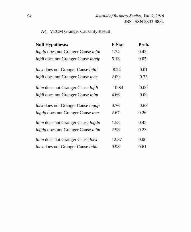
94 Journal of Business Studies, Vol. 9, 2016
JBS-ISSN 2303-9884
A4. VECM Granger Causality Result
Null Hypothesis: F-Stat Prob.
lngdp does not Granger Cause lnfdi 1.74 0.42
lnfdi does not Granger Cause lngdp 6.13 0.05
lnex does not Granger Cause lnfdi 8.24 0.01
lnfdi does not Granger Cause lnex 2.09 0.35
lnim does not Granger Cause lnfdi 10.84 0.00
lnfdi does not Granger Cause lnim 4.66 0.09
lnex does not Granger Cause lngdp 0.76 0.68
lngdp does not Granger Cause lnex 2.67 0.26
lnim does not Granger Cause lngdp 1.58 0.45
lngdp does not Granger Cause lnim 2.98 0.23
lnim does not Granger Cause lnex 12.37 0.00
lnex does not Granger Cause lnim 0.98 0.61
Journal of Business Studies, Vol. 9, 2016 95
JBS-ISSN 2303-9884
Visitors’ Perception towards Tour Destinations: A Study on
Padma Garden
Md. Abdul Alim 1
Rudrendu Ray 2
Dr. Md Enayet Hossain 3
Abstract
This empirical study is conducted to find out the visitor’s perception towards the
tour destination, Padma Garden, Rajshahi in Bangladesh. A convenient sampling
technique was used to collect data. Total thirty one quality attributes were taken
into consideration to find out the choice similarities or dissimilarities towards the
selected destination. A total 199 usable data were collected from Padma Garden
using 5 point Likert Scale. Data were analyzed using SPSS to find out influential
factors which are the most responsible for drawing the attention of the visitors.
Findings reveal six factors; food and beverage, price, accommodation,
environment, safety and security and transportation. However, food and beverage
is appeared as the most influential factor consisting six attributes whereas
transportation appears as less important to the visitors for visiting the destination.
The main contribution of the study is twofold. Theoretically it provides insightful
relationship between visitors’ choice factor and visiting to the destination.
Practically, the destination operators can use the mentioned factors in their
promotional activities.
Keywords: Visitors’ perception, tour destination, Padma garden
(I) Introduction
ourism is a rapid growing industry (Saayman et al., 2001) and has
been greatly contributing in many economies of the world. The
tourism industry generates enormous economic and noneconomic
benefits to both host country and tourists’ home countries. According to
the World Travel and Tourism Council (WTTC), the total contribution of
1 Assistant Professor, Department of Marketing, University of Rajshahi,
Email:[email protected] 2 Assistant Professor, Department of Marketing, University of Rajshahi,
Email:[email protected] 3 Professor, Department of Marketing, University of Rajshahi,
Email: [email protected]
T

96 Journal of Business Studies, Vol. 9, 2016
JBS-ISSN 2303-9884
travel and tourism to GDP was USD 7580.9 billion (9.8% of GDP) in
2014, and forecast to rise by 3.7% in 2015 and 3.8% in 2025. In
Bangladesh, although, the total contribution of Travel & Tourism to GDP
was BDT 627.9bn which was 4.1% of GDP in 2014, and is forecast to rise
by 6.0% in 2015 and 6.5% in 2025. The total contribution was 3.6% of
total employment which were 1984000 jobs in number in 2014 (WTTC,
2015).
There are different types of communities, specifically in developing
countries; indeed, tourism has represented a stronger connection to the
rich economic markets (Johnston, 2000; Rodriguez, 1999). In those
countries, tourism has a great contribution to change in household
economies, create new opportunities for employment, new sources of
liquid income, and new information about technologies (Barkin, 1996;
Eadington, & Smith, 1992; Levy and Lerch, 1991; Liu, 2003; Ahmed et
al., 2010). However, in tourism industry, tourism destination is one of the
most frequently used concepts but different stakeholders and tourism
researchers use it differently. In the tourism literature, destinations are
described as places, as regions and as images (Framke, 2002). A
destination abundant of natural resources and/or other attractions can give
competitive advantage (Crouch & Ritchie, 1999).
The advantages of tourism destinations are based on different products,
qualifying determinants of visitation, as well as the fundamental reasons
for potential visitors to choose one destination over another. In addition, a
tourist destination is a place which is very often visited by many locals,
national as well as international visitors. The tourism destination can be a
city, town, historical place, sea-beach, mountain, an amusement park,
museum or religiously important places. However, a park is regarded as a
large garden or area of land used for recreation. It has been recognized as
an important tourism and recreational resources to the local people and the
visitors come from the out of town (Buckley, 2000; Cho, 1988; Uysal,
Mcdonald, 1994). It could also be natural tourist attractions like forests,
rivers, big waterfalls, hills or lakes. It is rigorously studied that why these
destinations are important to the visitors particularly river based
destinations. On the contrary, people can make an ordinary place into an
important tourist destination by their own effort like making amusement

Journal of Business Studies, Vol. 9, 2016 97
JBS-ISSN 2303-9884
parks, statues, big hotels or by making a new city or town. Tourists have
different choices and that is why different tourists have different
perceptions towards a particular tour destination (Yeoman, 2008).
It is focused that different authors use the term perception in different
ways. It has emerged surrounding the concept and understanding of what
perception means. In this regard, one of the most widely accepted
definitions was defined by Berkman (2010): “Perception is the way in
which individual gathers, processes, and interprets information from the
environment”, and Gale (1994) stated that perceptions are the beliefs
about what a consumer received from the goods and services. Moreover,
perception has the substantial impact to the visitors for developing the
tourism industry. Mainly it is a process by which a person selects, sort out
and interpret the thing quickly into a meaningful picture of the
environment and accept the product in various ways; it may be favorably,
less favorably or not at all (Dey et al, 2012; Shamsuddin, & Hasan, 2013).
Again, the improvement of the cleanliness, safety and facilities of the
beach could be varying by the opinion and perceptions of the beach users
(Semeoshenkova & Williams, 2011). Thus, it is said that, recreational
services influence the visitors’ choice for selecting a particular tour
destination.
(II) Study Area
Bangladesh is one of the countries with a unique scenic beauty and rich
cultural heritage that she offers to the visitors from home and abroad.
Rajshahi is one of the divisional towns in Bangladesh and it is a growing
tourist destination in the country. The town is located on the bank of the
Padma River. Similarly, with this flourishing entertainment spot, we
foresee Padma Garden as the scope of employment opportunity for several
hundreds of people. It has also been ensured that the ways of earning of
livelihood of the employed by selling various items that the visitors feel a
need including fast-food, toys and flowers. Although the Padma river is
with a meager or without any water now due to diversion of water through
the Farakka Barrage across the border but the efforts of Rajshahi City
Corporation and some private entrepreneurs to turn its embankments and
surrounding land into a green zone with various trees and plants has made
Padma-Garden one of the most attractive places of the city.
98 Journal of Business Studies, Vol. 9, 2016
JBS-ISSN 2303-9884
During the last decade, the roads along the Padma-Garden has been
repaired, trees have been planted, various colorful tents with chairs and
benches for sitting and gossiping have been built and all the areas has been
linked with colorful electric bulbs and devices. Those who visited the
riverside a couple of years ago and visiting now will be surprised at the
first sight to watch its beauty and presence of a good number of visitors.
Although there is no statistical evidence of the number of visitors at
Padma Garden, but based on the observation of the researchers by visiting
the said destination, it could be around 2000 visitors visited at the said
destination per day particularly in the evening. However, in the first half
of the day visitors are quite less in number. It is probably due to the
working hours of the local visitors.
It is clear to us that, the contribution of Padma Garden in the local and
national economy of Bangladesh bears an important role. The flow of
economic contribution and the growth and sustainability depends on the
number of visitors’ arrival and facilities they consume. It can be explored
that how sufficient is the provided facilities of the responsible authorities
to the visitors. What is the visitors’ perception towards the various
qualities are to be understood. The purpose of the present study is to
investigate the visitors’ perception towards the quality services at Padma
Garden as a tour destination.
(III) Objective of the study
The main objective of the study is to find out the factors influencing
visitors’ perception towards the Padma Garden, Rajshahi as a tour
destination in Bangladesh.
In relation to the aforementioned objective, the specific objectives are as
follows:
i. To identify the different quality attributes that influence visitors to
select the Padma Garden as their tour destination.
ii. To understand how visitors’ perception varies based on various
factors.
(IV) Literature Review
Baloglu et al., (2003) conducted research on the relationship between
destination performance, overall satisfaction, and behavioral intention for

Journal of Business Studies, Vol. 9, 2016 99
JBS-ISSN 2303-9884
distinct segment. The purpose of this study was to gain a better
understanding of short-term visitors of mountain destinations in order to
improve marketing strategies. However, Chheang (2011) examines tourist
perceptions and experiences and argues that tourist perception is positive
and based on cultural enrichment, friendliness and the sense of hospitality
facilities of the local people experiences of the visitors are over than the
expectation. Kamal and Chowdhury (1993) and Hasan and Chowdhury
(1995) conducted studies on the basis of tourism related services. In fact,
these were the studies based on the performance of tourism related
services as well as the contribution to the development of the country’s
tourism industry. Therefore, Henderson (2011) highlighted other factors
that almost influence on inbound and outbound tourist to travel such as
political instability, safety and security and in terms of social
psychological concepts Higginbotham (2011) give emphasis on the
interrelated fields of recreation, leisure and tourism. Likewise, others
studies have been conducted by Hossain and Firozzaman (2003); Alam &
Shamsuddoha (2003); Hossain (2006); Lincoln (2008). These studies
focused that the significance of tourism is viewed from many angles e.g.
economic, social, cultural, political etc. Another study conducted by
Sofique and Parveen (2009) and Ahammed (2010) are directly related to
Cox’s Bazaar tourism regarding economic and socio-cultural effect of
tourism. This study is based on the factors that affect the visitors’
perception for selecting a tour destination. In this regard Ahmed et al.
(2010) conducted a study on factors affecting chooses Bangladesh as a
tourist destination. The study shows that service quality, natural beauty,
security and shopping facility are statistically significant in explaining the
intention for selecting a tour destination in Bangladesh (Cai & Zhang,
2003; Lee et al., 2004; Neal, 2003) and (Yourtseven, 2000) have
conducted research to meet the demand of tourism development. Here,
authors stated mainly of customer satisfaction and finding effective ways
to ascertain customer desire depends on status full occupation and
technically focused.
Food is very sensitive and one of the most priority issues in tourism as
well as services related industry (Donald, 1997). It is not only core value
of food but also packages of benefits -such as presentation of food, overall
environment of seating arrangement, way of approaching of service

100 Journal of Business Studies, Vol. 9, 2016
JBS-ISSN 2303-9884
providers etc (Cook et. al., 2007). However, at present food and beverage
are the common motivator of all kinds of existing and potential visitors’
and it is a ceiling trend in individuals mind for selecting a tour destination
(Ahmed et al., 2010).
Zeithaml (1988) defined price as what consumer sacrifice in order to gain
something from a product or services. Again, Berry and Parasuraman
(1991) emphasized on price as what customers actually pay in exchange
for products or services’ they received or a visible sign of services’ level
and quality. But in the destination perspective, Bagwell & Bernheim
(1996); Ngoc & Trinh (2015) describe price as what consumers are willing
to pay more for services at a destination if they think that prestigious
images are associated with it. In these cases, consumers feel interest in
paying higher price for effective goods which are associated with the
destination’s sophistication with greater perceived value (Papatheodorou,
2002).
Middleton and Clarke (1999) stated that accommodation has a functional
role for providing the facilities that makes travel convenient and
comfortable. Hall (1995) regarded accommodation as one of the most
critical components on the demand side as accommodation has a major
influence on visitors the type of who come to a destination. Cooper,
Fletcher, Gilbert and Wanhill (1996) suggested accommodation provides a
necessary support services to satisfy the broader motivation that brought
the visitor to the destination. Some authors (Chi & Qu 2008; Pike, 2009;
Ahmed et al., 2010) have mentioned that accommodation facilities are
most priority aspect for the visitors.
Hasan (1992) and Hall and Page (2000) conducted the four elaborate
studies covering the tourism and tourism environment in Bangladesh. The
study focuses tourism potentiality, major problems and prospects of
tourism, marketing strategies of tourism industry, foreign tourist arrival
trend in Bangladesh. For attracting the both domestic and international
visitors to the tourist destinations environment plays a significant role
(Dunn, 2009). An attitude towards the environment is a measure of how
people would like to experience the landscape based on their personal

Journal of Business Studies, Vol. 9, 2016 101
JBS-ISSN 2303-9884
preferences for environmental, social and cultural aspects. These
preferences reflect more basic values or environmental value orientations
Homer and Kahle (1988) and they are often related to the attitudes toward
specific environmental conditions and impacts as well as management and
development options.
In tourism industry safety and security is the synonym for providing
quality services, by ensuring that it helps visitors while thinking to choose
a destination. Tourism is different from any other economic activity;
visitors always seek safe and secure places to enjoy their pastime without
any tension. In this regard, Albrechtsen (2002) noted that “safety is the
protection from unintended incidents while security is the protection from
intended incidents”. Safety is concerned with human life and health’s
protection while security refers to the protection against criminal
activities. Therefore, success or failure of a tourism destination depends on
providing a safe and secure destination (Besculides et al., 2002). We
cannot be complacent, since there is an emerging consensus that crime -
which raises safety issues, is a growing concern among tourism
stakeholders who fear the potential damage that it may inflict on the
perception of safety and, by extension, the industry (Volker & Soree,
2002; Ahmed et al., 2010). However, in recent years researchers reported
that in country like Bangladesh visitors’ safety and security issues are
alarming to the travelers (Embassy Web-pages of America, Norway and
Denmark have been consulted in February 2006). In tourism, different
destinations required different levels of security e.g. safety and security
issue, visitors’ perception at Taj-Mahal is significant. But the Padma
Garden, on the other hand, is not that much of concern to both visitors and
the destination operators as well. Thus, minimum level of peaceful
surrounding environment and political stability of the country would be
the best concern to the local as well as domestic visitors. In this regard,
Lee et al., (2007) stated that safety and security system is not the same for
each destination.
It is difficult to run tourism industry without an effective and efficient
transportation system (Cook et al., 2007). Transport is the major cause for
tourism development and it has both positive and negative effects on
102 Journal of Business Studies, Vol. 9, 2016
JBS-ISSN 2303-9884
tourism. To start with, the improved facilities have stimulated tourism and
the expansion of tourism has stimulated transport. In this regards
accessibility is the key functions in the shadow of tourism transport. In
order to access the areas that are mainly aimed, tourists will use any
transportation mode. However, air transport is the main mode for
international tourism (Kroshus, 2003). However, in the context of
Bangladesh transportation facilities are not same for each destination
(Gallarza & Saurab, 2006).
A number of studies are reviewed including above and it is clear to us that
it seems a significant research gap existing in the domestic tourism market
in Bangladesh to ascertain visitors’ perception towards selection of a tour
destination. In previous academic research it was hardly given attention on
the country’s tourism industry. Thus, the present empirical study has an
opportunity to know new knowledge about this area. The present study
aims to gather primary data from the visitors at Padma Garden. This
research paper presents the relevant variables that are affecting to the
visitors’ perception in choosing a particular tour destination. Therefore,
the findings of this study will give new idea and the directions to the
concerned authorities to pace their competitiveness.
(V) Methodology
The study is carried out on Padma Garden, Rajshahi area in Bangladesh.
The reason for choosing this area is that it is the local amusing river based
visiting spot and there is no significant research carried out earlier about
the factors that greatly affect the visitors’ mind for selecting the
destination. Thus the authors interested to identify the factor that affects
the visitors’ perception to Padma Garden. This study mainly follows
positivist paradigm, the field study technique was used for data collection.
The main selection criterion is that the visitors must be on the spot during
interview. The sample population for this study is composed of visitors
who visited Padma Garden, Rajshahi through convenience sampling. It
mainly focuses on the areas of information needed to satisfy the objectives
of this research. Out of 225 sample questionnaire 199 usable questionnaire
were collected with a response rate of over 84% using 5 point Likert scale
ranging from 1 to 5 response categories. Mainly close ended questions
were used in the questionnaire. However, there were some open ended
Journal of Business Studies, Vol. 9, 2016 103
JBS-ISSN 2303-9884
questions used to collect demographic information from the respondents.
Largely factor analysis was used for the data analysis. Data were analyzed
using statistical software SPSS to find out the influential factors, which
would be most responsible for drawing attention of the visitors.
(VI) Discussion of Results
Respondents’ Profile
In this study, seven demographic characters have been observed by the
authors over those who visited Padma garden, Rajshahi. Among them
gender, age, profession, home district (place of residence of the visitors)
and the marital status have the significant differences in their counterpart.
Table 1 depicts the data that majority of the visitors are male (81.9%) and
rest of them are female (18.1). Two-third of the visitors’ age group is 21-
30 years (63.8%) whereas visitors over 50 years of age are only 1%;
probably it is due to their weak physical condition and mental
unwillingness. However, in terms of professional status, student carried
the lions’ share (62.8%) to visit the mentioned destination. These young
people have the curiosity to know and attention for utilizing their pastime
in an enjoyable and productive way. It is also observed that geographically
visitors from Rajshahi region have the significant intension to visit Padma
garden that is 62.3%. On the other hand, those form Barisal and Sylhet has
the least tendency to visit this local based visiting spot. Moreover,
precisely two-third of the visitors is unmarried. In addition to that, among
the visitors, educated people have the highest trend to visit Padma garden
where the percentage of graduate and post graduate is 43.2 and 33.7
respectively. Therefore, three-fourth of the visitors is well educated
coming from this city of education. Eventually, visitors or their parents’
monthly income is Tk. 10001-20000 and Tk. 20001-30000, which is
34.1% and 32.2% respectively. On the contrary, over tk. 30000 of income
group has less participation towards this amusing destination.
Measurement
In sampling adequacy author uses KMO and Bartlett’s test to examine the
sample accuracy. The result of Kaiser-Meyer-Olkin Measure illustrates
that the presented sample is quite suitable for factor analysis. (Table 2)
figures that current data is 89% accurate at with 99% significant level.

104 Journal of Business Studies, Vol. 9, 2016
JBS-ISSN 2303-9884
From the analysis of data, we find 31 quality variables out of the initially
approached 42 variables. These are important for examining the factors
that affect the visitors’ perception of Padma garden, Rajshahi in
Bangladesh. Based on Eigen value, all 31 variables are selected-value 1
considered into the list of variables. Statistically, 31 variables construct six
factors, which explain almost 60% of the field. So author concentrates on
these factors for the study. Factor 1 explains 31.889% where total Eigen
value is 9.886 (Table 3). With this rational cause, this factor is the top
most priority concern to the current study, which is related to the services
of food & beverage at Padma garden, Rajshahi.
Variables with loading higher than 0.5 are grouped under all factors.
However, factor loading is the correlation between the original variable
with the concerned factor and the key to understanding the nature of that
specific factor (Debasish, 2004). Table 4 has been supplied the Varimax
rotated factor loadings against the earlier mentioned 31 variables
consisting of 6 factors. Moreover, six factors components and the
correlations can be seen in rotating component matrix. Rotation has been
carried out through Varimax rotation method. SPSS (version 18) is used
for analysis. Factor 1 (food and beverage), Factor 2 (price), Factor 3
(accommodation facility), Factor 4 (environment), Factor 5 (safety and
security) and Factor 6 (transportation). However, the total variance
accounts for all the six factors which is 59.041 %.
Factor 1 (Food and Beverage): The study discovered that food and
beverage has great influence on visitors. This factor determines six items,
which is highly correlated with the first factor. However, the factor
loading score for each item is within the acceptable level (from 0.615 to
0.745; See Table 4). In this factor, the Cronbach’s alpha value 0.872
which is quite standard in acceptable level 0.70 or above (O’ Leary-Kelly
& Vokurka, 1998) and mean value of this individual factor is 3.492.
Considering the above mentioned score, the factor and the items are
relevant. As food and beverage is the prime attraction to the visitors to this
short trip destination, therefore destination operators can extend the list of
food items with different taste for getting more attention from the potential
visitors. However, keeping existing quality of the foods could be the first
priority to the authority of Padma Garden.
Journal of Business Studies, Vol. 9, 2016 105
JBS-ISSN 2303-9884
Factor 2 (Price): There are also six attributes that are the strong correlated
with this factor. In this regards, service charge at accommodation is
economy (0.696) and price of drinks (0.695). Moreover, the visitors’
perceived benefit in value of food charge and transportation cost is
satisfactory by 0.685 and 0.665 respectively. Furthermore, the cost of
natural sightseeing facilities and goods purchasing facilities are in within
the standard level at 0.658 and 0.647. In the factor analysis, this factor
brings alpha value (0.810) and mean value 3.313. Eventually, as the entire
price concerning item are ranging in minimum level so that it is rightly
constructed. Evidence from the demographic profile shows that, most of
the visitors of Padma Garden are student (62.8%) and approximately two-
third of the visitors or their parents’ monthly income is between Tk. 10001
to Tk. 30000. So that continuation of existing price of the destination
would be suitable to keep the continuous flow of the visitors.
Nevertheless, price of some of the items of this factor is not under control
by the destination operator such as price of drinks, transportation cost etc.
It depends on the country’s overall economic condition. So that it can be
an effective initiative for the planners to control their internal cost that
would led the sustainable growth of this destination.
Factor 3 (Accommodation Facility): Accommodation is one of the most
important basics to the visitors to visit any destination. The current study
identifies five variables where accommodation facility plays a functional
role to influence the visitors to visit this destination. The factor loading
score for each of the five items is within the acceptable range that is from
0.596 to 0.744 Such as physical condition of accommodation (0.744),
room service facilities at hotel (0.716), comfortability at room (0.689),
facilities for shopping in the destination area (0.608) and accommodation
at restaurants (0.596). However, the Cronbach’s alpha score (0.819) is
above the standard level and mean value 3.077. These scores clearly
indicate that the factor is justified. Thus, the destination operator and those
are involved in providing accommodation facilities can work together to
ensure the guests’ comfort at hotel and restaurant. Moreover, usually
shopping facilities at the destination area is not a major concern in this
local visiting spot rather their main intention is entertainment and
106 Journal of Business Studies, Vol. 9, 2016
JBS-ISSN 2303-9884
recreation. But unintentional purchase is the part of any kinds of visitors’
cultures particularly, some documentary materials such as- souvenirs and
statue with historical background and images of the destination. In this
case, the authority of the destination can pay their attention for expanding
the range of the products and services to meet the needs of the visitors and
can get extra money.
Factor 4 (Environment): Visitors always tend to seek a comfortable,
enjoyable and pleasant environment for their physical and mental
recreation. The existing study consists of five variables that are highly
correlated with the fourth (Environment) factor. Here visitors have
significant intension to natural environment and weather condition of the
garden that is scored by 0.744 and 0.687 respectively. On the other hand,
chaos free environment and image of the destination is 0.674 and 0.670
accordingly. However, political stability is 0.603. Where Cronbach’s alpha
value 0.776 and mean value of individual factor 3.570. Finally, author
combines this factor as influential because the items logically included
with the context of this green city Rajshahi. In fact, Rajshahi is blessed
and have privileges for its geographical location due to not threatened by
substantial natural disaster. So it is an opportunity to hold its existing
natural and artistic view of Padma Garden. Therefore, the planners and the
decision makers are suggested to enhance its greenage environment for
building a positive impression into the visitors’ mind, which will be
helpful in case of achieving competitive advantage in future.
Factor 5 (Safety & Security): it is often said that nothing can be enjoyable
if their remains insecurity in mind. Rationally, safety & security emerged
as the major concern to the visitors. The security issue is important indeed
for meeting the objectives i.e. recreation, entertainment etc of the visitors.
In this factor, four items considered by analysis ranging from 0.620 to
0.703 (See Table 4) where safety in cultural program and medical issue is
also included as significant variables. This factor is determined by
Cronbach’s Alpha score .803 and mean value 3.190. Therefore, due to
logical reason, the factor safety & security is valid. Safety and security
issues are the primary requirement to the visitors because people can go to
a place when he/she feel like being entertained. Thus, a visitor can get

Journal of Business Studies, Vol. 9, 2016 107
JBS-ISSN 2303-9884
pleasure and full charm of recreation when he feels secured. According to
the study result, as rate of gathering is higher in the evening even or even
at night, authority of Padma garden can take a measure through their own
security system to receive more attention from the visitors.
Factor 6 (Transportation): There are five quality attributes that are strongly
correlated except the one (safety in internal transportation). The acceptable
level of items-road transport facility, internal transportation and water
transportation which is 0.674, 0.537 and 0.530 accordingly. However,
efficiency in public transportation is 0.524. The Cronbach’s Alpha is
0.793 and mean value of this single factor is 3.329. But, safety in internal
transportation is scored by 0.434 which seems under the minimum
acceptable level. Moreover, author emphasis on this factor since data were
collected from field sources. In this destination twofold transportation
facilities required to the visitors that are internal and external. In case of
external- destination authority doesn’t have control over them. However,
internally it has high demand to pay attention to make the right balance of
happiness of the visitors. In particular, as this destination has built based
on the Padma River and moving on the river by boat is the key attraction
to the visitors for their adventure. But in the rainy season, water overflows
on the river and it creates big weaves. Therefore, boats, the only way of
water transportation, fall in danger and post incident recovery measure is
inadequate. In this case, the planners, policy makers and the authority of
Padma Garden are strongly encouraged to take immediate steps to launch
live support boat for the visitors’ safety & security.
(VII) Conclusion
The main purpose of this study is to find out different aspects of Padma
garden at Rajshahi that attract visitors. In this study, it is clearly seen that
visitors are attracted towards Padma Garden because of several factors
among which food and beverage is the highest in preference. Thirty one
quality variables have been found and each variable is different from
another. As a result, the authority of this destination can be suggested to
make item wise customized promotional activities. In addition to that, it
would be much better to reconstruct all the factors for the visitors of
moderate economic status especially for students. Because, a certain group
of visitors have least tendency to visit this destination those are
108 Journal of Business Studies, Vol. 9, 2016
JBS-ISSN 2303-9884
economically strong. On the other hand, in order to get nationwide
attention from expectant visitors, concerned authority is also advised to
make smooth harmony with the other destinations at Rajshahi. As bunch
of attractions are available at Rajshahi such as Varendra Research
Museum, different renowned educational institutions including Rajshahi
University. Visitors would be able to get the pleasure of different places in
a single city. As a result, not only domestic visitors but also international
visitors would be interested to visit this excellent destination with full of
natural beauty. In this case, shopping could be one of the most leading
attractions to the visitors as the country’s best silk factories are situated
here in this city whether domestic or international visitors can collect silk
items directly whether from the showroom or the factory.
References
Ahammed, Sheikh Saleh, (2010). “Impact of Tourism in Cox’s Bazar,
Bangladesh” Master’s Thesis, Master in Public Policy and Governance
Program, Department of General and Continuing Education, North South
University, Bangladesh.
Ahmed Feroz., Azam, Shah & Kanti, T.B. (2010). “Factors Affecting the
Selection of Tour Destination in Bangladesh: An Empirical Analysis”
International journal of Business and Management, Vol 5, No3, March
2010.
Albrechtsen, E. (2002). A generic comparison of industrial safety and
information security. Term paper in the PhD course "Risk and
Vulnerability", NTNU. [Online]. Available at http://www.iot.ntnu.no/
users/albrecht/rapporter/generic%20comparision%20of%20ind%20saf%
20and%20inf%20sec.pdf
Alegre, J. & Juaneda, C. (2006). Destination Loyalty, Consumers’ Economic
Behavior. Annals of Tourism Research, Vol. 33(3), pp. 684-706.
American Embassy. http://www.infozee.com/usa/embassies/bangladesh.htm-Dhaka,
Bangladesh. Accessed on the 30th of December 2010.
Bagwell, S.L. & Bernheim, D.B. (1996). “Veblen effects in a theory of
conspicuous consumption,” The American Economic Review, Vol. 86,
No. 3, pp. 349-373.
Journal of Business Studies, Vol. 9, 2016 109
JBS-ISSN 2303-9884
Baloglu, S., Pekcan, A., Chen, S-L. & Santos, J. (2003).The relationship between
destination performance, overall satisfaction, and behavioral intention for
distinct segment. Journal of Quality Assurance in Hospitality & Tourism,
17(1), 149-165. [Online] Available: http://www.haworthpress.com/
web/JQAHT (Accessed 10-10-2006).
Barkin, D. (1996). Ecotourism: A tool for sustainable development in an era of
international integration. In J.A. Miller and E. Malek-Zadeh (Eds), The
Ecotourism Equation: Measuring the Impacts (pp. 263–272). New
Haven, CT: Yale University.
Berry, L.L. & Parasuraman, A. (1991). Marketing Services: Competing through
Quality.: New York: Free Press.
Besculides, A., Lee, M.E. & McCormick, P.J. (2002). Residents’ perceptions of
the cultural benefits of tourism. Annals of Tourism Research, 29 (2):
303–319.
Buckley, R. (2000). Neat trends: Current issues in nature, eco- and adventure
tourism. International Journal of Tourism Research, 2: 437–444.
Cai, L.A. & Zhang, L. (2003). Meeting the demand from tourism development–
higher occupation and technical education in China. Journal of Human
Resources in Hospitality & Tourism, 3(1), 106-117. [Online] Available:
http://www.haworthpress.com/web/JTTM (Accessed 22-10-2006).
Campbell, L.M. (1999). Ecotourism in rural developing communities. Annals of
Tourism Research, 26(3): 534–553.
Chheang, V. (2011). Angkor Heritage Tourism and Tourist Perception.
Tourisms: An International Multidisciplinary Journal of Tourism, Vol. 6,
No.2, pp.213-240.
Chi, G.O.C. & Qu, H. (2008). Examining the Structural Relationships of
Destination Image, Tourist Satisfaction and Destination Loyalty: An
Integrated Approach. Tourism Management, Vol. 29, pp. 624-636.
Cho, G. (1988). Conservation and management in Jervis Bay Australia. Aquatic
Conservation: Marine and Freshwater Ecosystems, 8, 701–717.
Cook, R.A., Yale, L.J. & Marqua, J.J. (2007). Tourism –The Business of Travel.
Delhi: Pearsons Publication.
Cooper, C., Fletcher, J., Gilbert, D. & Wanhill, S. (1996). Tourism Principles
and Practice, London: Longman
Crouch, G.I. & Ritchie, J.R.B. (1999). Tourism, competitiveness, and societal
prosperity. Journal of Business Research, Vol. 44, pp. 137-152.
110 Journal of Business Studies, Vol. 9, 2016
JBS-ISSN 2303-9884
Dey, P. et al., Tourists Perception towards Cox’s Bazar Sea Beach in Bangladesh
as a Tourist Destination (2012). Asian Business Review, Volume 2,
Number 1/2013 (Issu 3) ISSN 2304-2613 (Print); ISSN 2305-8730
(Online).
Dunn, K.C. (2009). Contested State Spaces: African National Parks and the State.
European Journal of International Relations, 15(3): 423-446.
Eadington, W.R. & Smith, V.L. (1992). Tourism Alternatives: Potentials and
Problems in the Development of Tourism. Philadelphia, PA: University
of Pennsylvania Press.
Embassy of Denmark, Dhaka Bangladesh http://www.ambdhaka.um.dk/en
Embassy of Norway in Bangladesh http://www.norway.org.bd/info/embassy.htm
Framke, W. (2002). The Destination as a Concept: A Discussion of the Business-
related Perspective versus the Sociocultural Approach in Tourism
Theory. . Scandinavian Journal of Hospitality and Tourism, Vol. 2(2),
pp. 92-108.
Gale, B.T. (1994). Managing Customer Value, The Free Press: New York, NY.
Gallarza, M.G. & Saurab, I.G. (2006). Value dimensions, perceived value,
satisfaction and loyalty: an investigation of university students’ travel
behavior. Tourism Management,, Vol. 27, pp. 437-452.
Hall, C. (1995). Introduction to Tourism: Development. (2nd Ed.). Melbourne:
Longman Cheshire.
Hasan, S.R. & Chawdhury, A.I. (1995). “Hotel and Restaurant Services and the
development of tourism in Bangladesh”, Journal of Business Studies,
Dhaka University. 14(1): 47-67
Hasan, S.R. (1992). Problems and Prospects of Bangladesh Tourism Industry in
Bangladesh, Bureau of Business Research, University of Dhaka, pp. 14-
15.
Henderson, J.C. (2011). Tourism Development and Politics in the Philippines.
Tourisms: An International Multidisciplinary Journal of Tourism, Vol. 6,
No. 2, pp. 159-173.
Higginbotham, G. (2011). Assisted-Suicide Tourism: Is it tourism? Tourisms: An
International Multidisciplinary Journal of Tourism, Vol. 6, No. 2, pp.
177-185.
Johnston, A. (2000). Indigenous peoples and ecotourism. Tourism Recreation
Research, 25(2): 89–96.

Journal of Business Studies, Vol. 9, 2016 111
JBS-ISSN 2303-9884
Kamal, M.M. & Chowdhury, A.l. (1993). “Marketing Orientation in Tourism
Sectors: Case Study of Biman Bangladesh Airlines”, Journal of Business
Studies, Dhaka University. 14(1): 47-67.
Kroshus, M.L. (2003). Commoditizing culture. Tourism and maya identity.
Annals of Tourism Research, 30(2): 353–368.
Levy, D.E. & Lerch, P.B. (1991). Tourism as a factor in development:
Implications for gender and work in Barbados. Gender and Society, 5:
67–85.
Liu, Z. (2003). Sustainable tourism development: A critique. Journal of
Sustainable Tourism, 11(6): 459–475.
MacDonald, S. (1997). A people’s story: Heritage, identity and authenticity. In
C. Rojek and J. Urry (eds.) Touring Cultures. Transformations of Travel
and Theory (pp. 155–175), London: Routledge.
Mir Sofique Abdul and Jannat Ara Parvin, (2009). “Economic Prospects and
Constraints of Cox’s Bazar Bangladesh – A Study”, South Asian Journal
of Tourism and Heritage (2009), Vol. 2, No. 1.
Neal, J.D. (2003). The effect of length of stay on travelers’ perceived
satisfaction with service quality. Journal of Quality Assurance in
Hospitality & Tourism, 17(1): 167-176. [Online] Available:
http://www.haworthpress.com/web/JQAHT. (Accessed on 10-10-2006).
Ngoc, M.K. & Trinh, T.N. (2015). Factors Affecting Tourists’ Return Intention
towards Vung Tau City, Vietnam – A Mediation Analysis of Destination
Satisfaction. Journal of Advanced Management Science Vol. 3, No. 4,
December 2015. pp. 292-298.
O’Leary-Kelly S.W. & Vokurka, R.J. (1998). The empirical assessment of
construct validity. Journal of operation management, 16(4): 387-405.
Papatheodorou, A. (2002). “Civil aviation regimes and leisure tourism in
Europe,” Journal of Air Transport Management, Vol. 8, No. 6, pp. 381-
388.
Parvin, N. & Chowdhury, H.K. (2006). Consumer Evaluation of Beautification
Products: Effect on Extrinsic Cues. Asian Academy of Management
Journal,, Vol. 11(2), pp. 89-104.
Petrick, J.F. (2004a). Are loyal Visitors’ Desired Visitors? Tourism
Management,, Vol. 25, pp. 463-470.
Pike, S. (2009). Destination Brand Positions of a competitive set of near-home
destinations. Tourism Management, Vol. 30, pp. 857-866.
112 Journal of Business Studies, Vol. 9, 2016
JBS-ISSN 2303-9884
Rao, A.R. & Monroe, K.B. (1988). The Moderating Effect of Prior Knowledge
on Cue Utilization in Product Evaluations. Journal of Consumer
Research,, Vol. 15, pp. 253-264.
Rodriguez, A. (1999). Kapawi: A model of sustainable development in
Ecuadorean Amazonia. Cultural Survival Quarterly, 23: 43–44.
Saayman, M., Saayman, A. & Rhodes, J.A. (2001). Domestic tourist spending
and economic development: the case of North West Province.
Development Southern Africa, 18/4: 443-455.
Uysal, M., McDonald, M. & Martin (1994). Australian visitors to US national
parks and national area. International Journal of Contemporary
Hospitality Management, 6(3): 18–24.
Volker, S. & Soree, J. (2002). Fighting over tourists: A case study of competing
entrepreneurs in a small town in Belize. In H. Dahles and L. Keune (eds),
Tourism Development and Local Participation in Latin America
(pp.101–114), New York: Cognizant Communications Corporation.
Williams, V.S. (2011). Beach quality assessment and management in the
Sotavento (Eastern) Algarve, Portuga. 1282-1286.
WTTC. (2015). World Travel and Tourism Council: Travel & Tourism
Economic Impact-2015.
Yourtseven, H. & Jencturk, A. (2000). Measuring and managing service quality
of ANZAC day as a cultural heritage event. Onsekiz University. [Online]
Available: http://[email protected], page-166.
Zeithaml, V. (1988). Consumer perceptions of price, quality, and value: a means-
end model and synthesis of evidence. Journal of marketing, Vol. 52(3),
pp. 2-22.
Zeithaml, V.A., Berry, L.L. & Parasuraman, A. (1996). The Behavioural
Consequences of Service Quality. Journal of Marketing,, Vol. 60, pp. 31-
46.
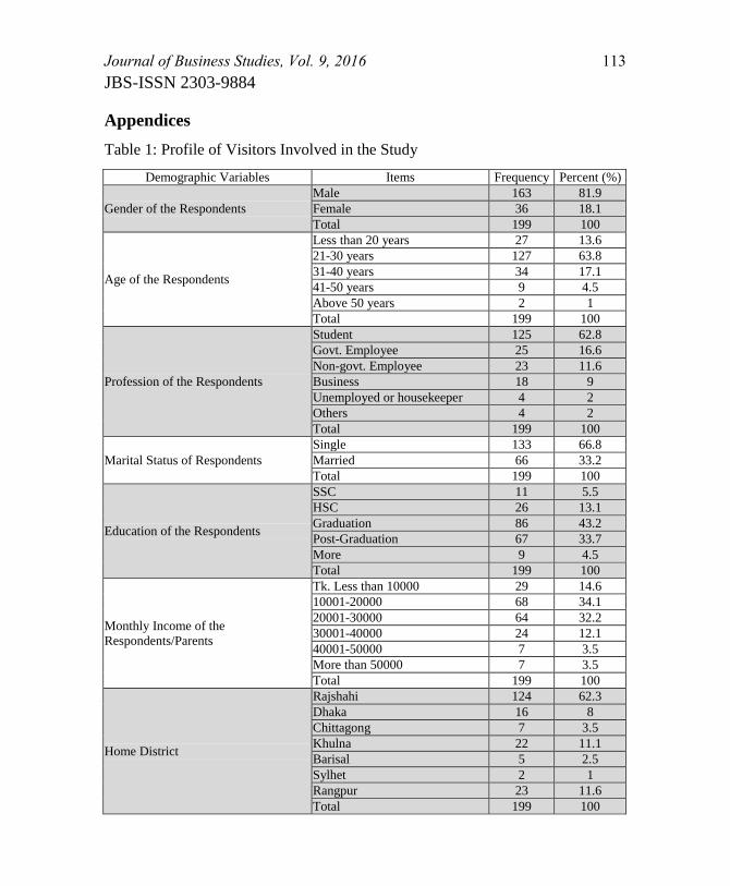
Journal of Business Studies, Vol. 9, 2016 113
JBS-ISSN 2303-9884
Appendices
Table 1: Profile of Visitors Involved in the Study
Demographic Variables Items Frequency Percent (%)
Gender of the Respondents
Male 163 81.9
Female 36 18.1
Total 199 100
Age of the Respondents
Less than 20 years 27 13.6
21-30 years 127 63.8
31-40 years 34 17.1
41-50 years 9 4.5
Above 50 years 2 1
Total 199 100
Profession of the Respondents
Student 125 62.8
Govt. Employee 25 16.6
Non-govt. Employee 23 11.6
Business 18 9
Unemployed or housekeeper 4 2
Others 4 2
Total 199 100
Marital Status of Respondents
Single 133 66.8
Married 66 33.2
Total 199 100
Education of the Respondents
SSC 11 5.5
HSC 26 13.1
Graduation 86 43.2
Post-Graduation 67 33.7
More 9 4.5
Total 199 100
Monthly Income of the
Respondents/Parents
Tk. Less than 10000 29 14.6
10001-20000 68 34.1
20001-30000 64 32.2
30001-40000 24 12.1
40001-50000 7 3.5
More than 50000 7 3.5
Total 199 100
Home District
Rajshahi 124 62.3
Dhaka 16 8
Chittagong 7 3.5
Khulna 22 11.1
Barisal 5 2.5
Sylhet 2 1
Rangpur 23 11.6
Total 199 100
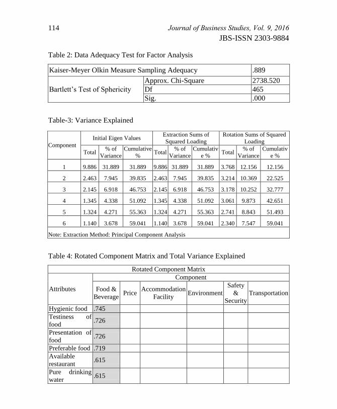
114 Journal of Business Studies, Vol. 9, 2016
JBS-ISSN 2303-9884
Table 2: Data Adequacy Test for Factor Analysis
Kaiser-Meyer Olkin Measure Sampling Adequacy .889
Bartlett’s Test of Sphericity
Approx. Chi-Square 2738.520
Df 465
Sig. .000
Table-3: Variance Explained
Table 4: Rotated Component Matrix and Total Variance Explained
Rotated Component Matrix
Attributes
Component
Food &
Beverage Price
Accommodation
Facility Environment
Safety
&
Security
Transportation
Hygienic food .745
Testiness of
food .726
Presentation of
food .726
Preferable food .719
Available
restaurant .615
Pure drinking
water .615
Component
Initial Eigen Values Extraction Sums of
Squared Loading
Rotation Sums of Squared
Loading
Total % of
Variance
Cumulative
% Total
% of
Variance
Cumulativ
e % Total
% of
Variance
Cumulativ
e %
1 9.886 31.889 31.889 9.886 31.889 31.889 3.768 12.156 12.156
2 2.463 7.945 39.835 2.463 7.945 39.835 3.214 10.369 22.525
3 2.145 6.918 46.753 2.145 6.918 46.753 3.178 10.252 32.777
4 1.345 4.338 51.092 1.345 4.338 51.092 3.061 9.873 42.651
5 1.324 4.271 55.363 1.324 4.271 55.363 2.741 8.843 51.493
6 1.140 3.678 59.041 1.140 3.678 59.041 2.340 7.547 59.041
Note: Extraction Method: Principal Component Analysis

Journal of Business Studies, Vol. 9, 2016 115
JBS-ISSN 2303-9884
Rotated Component Matrix
Attributes
Component
Food &
Beverage Price
Accommodation
Facility Environment
Safety
&
Security
Transportation
Service charge
at
accommodation
.696
Price of drinks .695
Value of food
charges .685
Price charge for
transportation .665
Price charge of
natural sight .658
Price charge for
buying goods .647
Physical
condition of
accommodation
.744
Room service
facility .716
Room's
comfort ability .689
Shopping
facilities .608
Restaurant at
accommodation .596
Natural
environment .744
Weather
condition of the
garden
.687
Chaos free
environment .674
Image of
destination .670
Political
stability .603
Safety in
cultural
program
.703
Safety at hotel .688
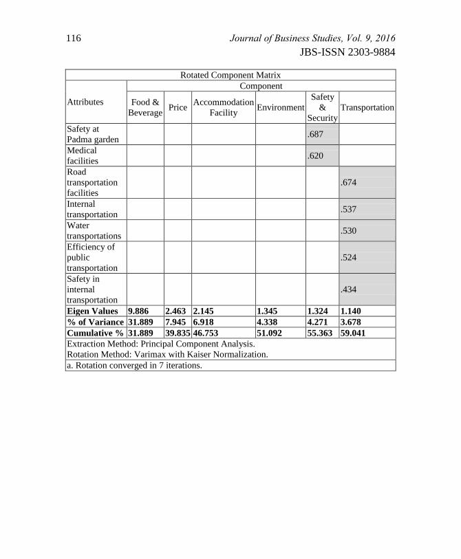
116 Journal of Business Studies, Vol. 9, 2016
JBS-ISSN 2303-9884
Rotated Component Matrix
Attributes
Component
Food &
Beverage Price
Accommodation
Facility Environment
Safety
&
Security
Transportation
Safety at
Padma garden .687
Medical
facilities .620
Road
transportation
facilities
.674
Internal
transportation .537
Water
transportations .530
Efficiency of
public
transportation
.524
Safety in
internal
transportation
.434
Eigen Values 9.886 2.463 2.145 1.345 1.324 1.140
% of Variance 31.889 7.945 6.918 4.338 4.271 3.678
Cumulative % 31.889 39.835 46.753 51.092 55.363 59.041
Extraction Method: Principal Component Analysis.
Rotation Method: Varimax with Kaiser Normalization.
a. Rotation converged in 7 iterations.
Journal of Business Studies, Vol. 9, 2016 117
JBS-ISSN 2303-9884
Determinants of Share Prices in Bangladesh: Evidence from
Pharmaceuticals Industry
Ajit Kumar Ghose 1
Md Solaiman Chowdhury 2
Abstract
The main focus of this paper is to examine the micro factors as the determinants
of share prices in Bangladesh. The study employs annual panel data over the
period of 2010-2014 pharmaceuticals sectors in Bangladesh. The results revealed
that the dividend per share, size and price earnings ratio have a positive and
significant impact on the share prices of pharmaceuticals sectors. The evidence
also shows that earning per share and return on equity are the crucial
determinants and positively associated with share prices. Moreover, the net asset
value per share positively influences the share prices of pharmaceuticals sector.
Keywords: Panel data, determinants of stock prices, pharmaceuticals sector
(I) Introduction
hare prices of a firm changes every now and then. Because of this
volatility, it is often hard to choose the right investment decision. The
changes in share price is influenced by a number of factors, if these factors
could be identified, it would be much easier for investors to choose the
right share to invest. Different school of thoughts have argued about the
determinants of share price. Some economist (e.g., Ohlson,1995) believe
that share prices are determined by the fundamental factors of a firm,
which are often called as the “micro factor”. Dividend Discount Model
(DDM), Binomial Pricing Model, Residual Income Valuation (RIV) and
Discounted Cash Flows (DCF) are some of the models which recognize
micro factors as the share determinants. While some other economists
(e.g., Sharpe,1964) believe that the share prices are determined by macro-
economic variables. Capital Asset Pricing Model (CAPM), Arbitrage
Pricing Theory (APT) are based on this ideology. On the contrary Keynes
1 MBA Graduate, Department of Finance, University of Rajshahi
Email: [email protected] 2 Assistant Professor, Department of Management Studies, University of
Rajshahi Email: [email protected]
S
118 Journal of Business Studies, Vol. 9, 2016
JBS-ISSN 2303-9884
(1936) holds that stock valuation is not a prediction but a convention,
which serves to facilitate investment and ensure that stocks are liquid,
despite being underpinned by an illiquid business and its illiquid
investments. Keynes (1936) explains price fluctuations in equity markets
by providing fictional beauty contest theory.
"It is not a case of choosing those [faces] that, to the best of one's
judgment, are really the prettiest, nor even those that average opinion
genuinely thinks the prettiest. We have reached the third degree where we
devote our intelligences to anticipating what average opinion expects the
average opinion to be. And there are some, I believe, who practice the
fourth, fifth and higher degrees." (Keynes, 1936, page-149).
Keynes believed that similar behavior was at work within the market. This
means micro and macro factors are not the determinants of share price.
Instead, what most people think their value is, will set the share price.
From the above arguments, it is quite clear that determination of share
price is an inconclusive issue in corporate finance. In Bangladesh, very
few research has been done on this topic (discussed in literature review).
In 2010-11, Dhaka stock exchange(DSE) collapse small investors were
greatly hit. Because of this incident and lack of sufficient research on
share price determinants, the authors are motivated to examine the issue.
The present study attempts to analyze the determinants of share price of
Pharmaceuticals sectors in Bangladesh. The objective is to identify the
relationships among firm fundamental factors (e.g., net asset value per
share, dividend per share, earning per share, firm size, return on equity,
price earnings ratio) of firm on DSE stock price. In the light of the above-
mentioned objective, the remaining part of this study is structured as
follows. In the next Section relevant literature is reviewed, later Section is
followed by study hypothesis and framework and methodology. The
Second last sections provide empirical results and discussions of major
findings and the final Section offers conclusion of this study.
(II) Literature Review
A good number of academic studies have tried to find key determinants of
share price. Determinants of share price vary among the academic
Journal of Business Studies, Vol. 9, 2016 119
JBS-ISSN 2303-9884
research due to difference in countries studied, market, methodology, and
study period. To investigate determinants of share price, a number of
related research papers have been reviewed in this section.
Zahir et al. (1982)studied the determinants of stock prices in India in 101
industrial giants in the private sector for the year 1976-77 and 1977-78
using multiple linear regression model. They found that dividend per share
emerged as a significant determinant of share price, dividend yield also
emerged highly significant determinant with its negative association with
market price of share. Balkrishan (1984)in his work analyzed the
relationship in the internal factor, i.e. dividend per share, earning per
share, book value, yield with market price of share. A linear regression
model was used to study the relationship of these variables in general
engineering and cotton textile industries. Book value per share and
dividend per share turned out to be the most significant determinants of
market price in both the industries.
Sharma (2011) investigated impacts of fundamental also known as micro
factors including-book value per share, dividend per share, earning per
share, price earnings ratio, yield, dividend payout, and size in terms of sale
and net worth on share price in Indian stock market for the period 1993-94
to 2008-09. He found that book value per share, dividend per share,
earning per share has positive impact on share price.
Srinivasan (2012) identified the fundamental determinants of share prices
in India. The study focuses on six major sectors of Indian economy
namely manufacturing, pharmaceutical, energy, infrastructure, commercial
banking sectors, information technology(IT) and information technology
enabled services (ITES) over the period 2006-2011. Random effects
model has been employed and found that earnings per share and price-
earnings ratio are the crucial determinants of share prices of
manufacturing, pharmaceutical, energy, infrastructure and commercial
banking sectors. The findings indicate that size is a significant factor in
determining the share prices of all sectors under consideration except
manufacturing. Moreover, the book value per share positively influences
the share prices of pharmaceutical, energy, IT and ITES and
Infrastructure. Uddin et al. (2013) examined the impact of internal factors
120 Journal of Business Studies, Vol. 9, 2016
JBS-ISSN 2303-9884
on stock prices of the companies in financial sector in Bangladesh over the
period 2005- 2011. By using multiple regression analysis, this study
revealed that earnings per share, net asset value, net profit after tax and
price earnings ratio have strong positive relationship with stock prices.
Bhattarai (2014) investigated the determinants of market stock price of
Nepalese Commercial Banks over the period 2006 to 2014. This study
revealed that earnings per share and price-earnings ratio have significant
positive association with share price while dividend yield showed
significant inverse association with share price of banks.
Malik et al. (2014) attempted to explain determinants of share price using
Ohlson (1995) model. According to Ohlson (1995) model book value per
share, earning per share and multiplication of book value per share and
earning per share are the key determinants of share price. Statistical
investigation using fixed effect model shows strong evidence for
applicability of Ohlson model for Karachi Stock Exachange listed
companies.
Jatoi et al. (2014) attempted to explain the share price changes due to only
one micro factor (earning per share) in cement industry of Pakistan over
the period 2009-2013.They used two variable linear regression model and
found that significant positive relationship exists between share price and
earning per share. Almumani (2014) determined the relationship between
Amman stock markets’ stock prices and different quantitative factors.
Results show that six internal factor (e.g., dividend per share, earnings per
share, book value, dividend payout ratio, price earnings ratio and size)
influence Amman stock markets’ stock prices. Applying ratio analysis,
correlation and a liner multiple regression models, this study found that
book value, earnings per share and price earnings ratio have positive
impact on share price of the listed banks in Amman stock exchange over
the study period 2005-2011. The study also found that size has inverse
relationship with share price and other variables such as dividend per
share and dividend payout have insignificant impact on share price.
The study of Arshad et al. (2015) examined the impact of different internal
and external factors that influence the share prices. They conducted their
study on commercial banks in Pakistan over the period 2007-2013. By

Journal of Business Studies, Vol. 9, 2016 121
JBS-ISSN 2303-9884
using linear multiple regression analysis, they found that earnings per
share has more influence on share prices and has positive and significant
relationship with share prices. Book to market value ratio and Interest rate
have also significant but negative relation with share prices while other
variables (gross domestic product, price earnings ratio, dividend per share,
and leverage) have no relationship with share prices.
The study of Iqbal et al. (2015) identified the fundamental factors that
affect stock price in Oil and Gas and Cement Sector of Karachi Stock
Exchange over the period 2008-2011. By using panel data approach, they
found that earnings per share and book value per share have positive and
significant impact on share price in both sectors. On the other hand,
dividend yield is negatively significant in only cement sector.
(III) Study Hypothesis and Framework
The literature reviewed earlier suggest strong evidence of relationship
between firm specific factors also known as micro factors and share price.
In view of theory and major empirical evidence market share price may be
influenced by net asset value per share, dividend per share, earnings per
share, firm size, return on equity, price earnings ratio. The following
hypothesis and conceptual framework (Figure 1) are developed to test the
effect of these variable on share price in DSE.
H0 = There is no significant influence of Net Asset Value Per
Share(NAVPS), Dividend Per Share(DPS), Earnings Per Share(EPS),
Firm Size(SIZE), Return on Equity(ROE) and Price Earnings Ratio(P/E)
on Share Price.
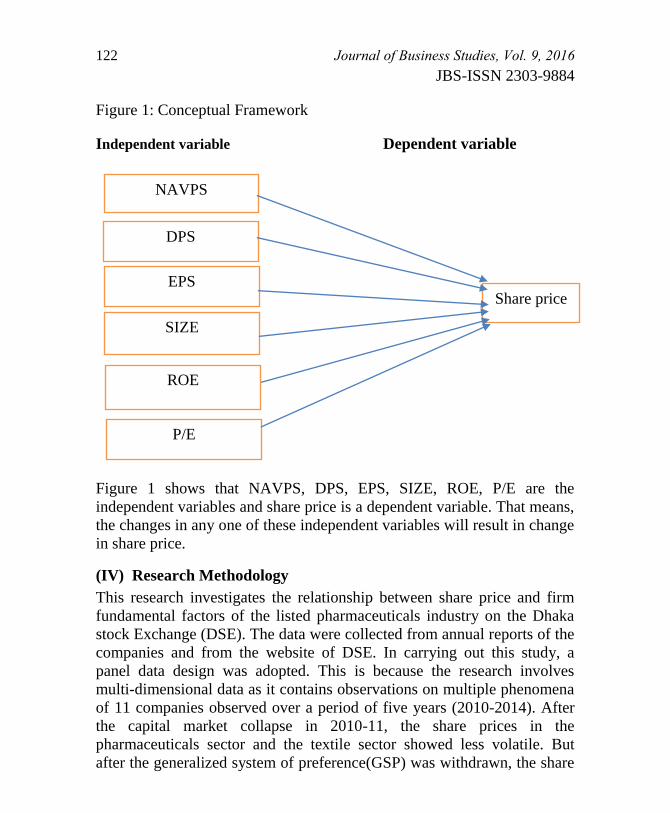
122 Journal of Business Studies, Vol. 9, 2016
JBS-ISSN 2303-9884
Figure 1: Conceptual Framework
Independent variable Dependent variable
Figure 1 shows that NAVPS, DPS, EPS, SIZE, ROE, P/E are the
independent variables and share price is a dependent variable. That means,
the changes in any one of these independent variables will result in change
in share price.
(IV) Research Methodology
This research investigates the relationship between share price and firm
fundamental factors of the listed pharmaceuticals industry on the Dhaka
stock Exchange (DSE). The data were collected from annual reports of the
companies and from the website of DSE. In carrying out this study, a
panel data design was adopted. This is because the research involves
multi-dimensional data as it contains observations on multiple phenomena
of 11 companies observed over a period of five years (2010-2014). After
the capital market collapse in 2010-11, the share prices in the
pharmaceuticals sector and the textile sector showed less volatile. But
after the generalized system of preference(GSP) was withdrawn, the share
Share price
NAVPS
EPS
DPS
SIZE
ROE
P/E
Journal of Business Studies, Vol. 9, 2016 123
JBS-ISSN 2303-9884
prices of the textile sector became volatile. So, the pharmaceuticals sector
was the only sector to show stability in share price. Because of this
stability pharmaceuticals sector is purposively chosen.
Table 1: Pharmaceuticals companies used in this study
ACI ORIONINFU
ACIFORMULA PHARMAID
AMBEEPHA RECKITTBEN
GLAXOSMITH RENATA
IBNSINA SQURPHARMA
LIBRAINFU
Table 1 shows the list of the companies used in this study and it is
arranged in alphabetic order. In achieving the objective of this study, we
use ordinary least square (OLS) method. The Hausman test was applied to
choose the most efficient and most suitable method between fixed and
random effect. Pearson product moment Correlation coefficient was also
used, first to conduct the multicollinearity test for all the independent
variables and then to determine the degree and strength of association
between the variables.
(V) Empirical Results
Table 2 provides a summary of the descriptive statistics of the dependent
and independent variables for 11 pharmaceuticals companies for a period
of five years from year 2010 to2014 with a total of 55 observations. The
table 2 includes the mean, median, standard deviation, number of
observations, minimum and maximum for the independent and dependent
variables of the model.
The mean of share price(SP) was 455.72 in Bangladeshi taka(BDT) and
the standard deviation was 461.51. This means, the average share price of
the pharmaceuticals companies in Bangladesh, under the period of study,
was 455.72BDT. Regarding the standard deviation, it means the value of
124 Journal of Business Studies, Vol. 9, 2016
JBS-ISSN 2303-9884
share price can deviate from its mean by 461.51BDT.The average value of
NAPVS was 212.54BDT. This implies that on average, the
pharmaceuticals company book value per share was 212.54BDT over the
study period. The maximum value of NAVPS for the study period was
1571.50BDT and a minimum value of 7BDT. The standard deviation was
436.36. Regarding the dividend per share, mean of dividend per share the
sampled firms was 7.84. It reveals that average yearly cash dividend was
nearly 78.4 percent of the face value of share price of sampled
pharmaceuticals companies. The highest dividend per share a company in
a particular year was paid 55 and in the same way the minimum ratio for a
company in a year was 1.
Moreover, EPS has a mean of 14.52 with maximum 68.63 and minimum
6.98. Minimum EPS (negative) is an indication that some firms incurred
loss during the study period, while the maximum is a clear indication that
some firms were able to generate profit.
Further, to check the size of the pharmaceuticals company and its
relationship with share price, natural logarithm of total market
capitalization was used as proxy. The mean of the natural logarithm of
market capitalization over the period 2010 to 2014 was 22.19 and standard
deviation of 2.04. The maximum value was 26.11 while the minimum
value was 17.69. To check profitability and its relationship with the share
price, ROE was used as a proxy. The average profitability was 18 percent.
This means, on the average, for each 1 BDT investment in equity of
pharmaceuticals companies there was 0.18 BDT return. The maximum
value of ROE for the year was 0.84 whereas the minimum value was -
0.04. Also, the standard deviation was 0.15 which indicates there was low
a variation from the mean.
Finally, the average value of the price earnings ratio was 37.27. That is,
average share price was 37.5 multiple of average EPS. The maximum
value and the minimum value was 135.85 and .05 respectively for the
study period.
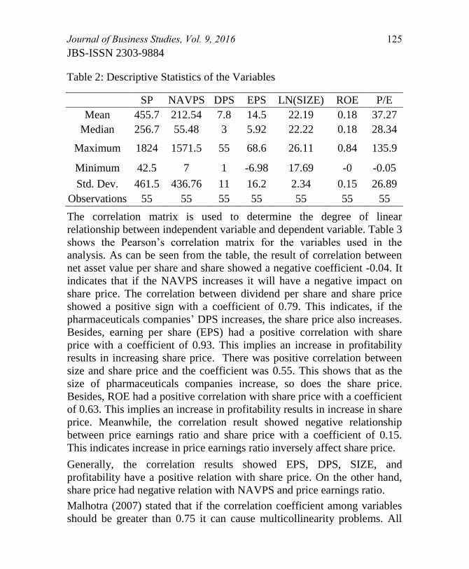
Journal of Business Studies, Vol. 9, 2016 125
JBS-ISSN 2303-9884
Table 2: Descriptive Statistics of the Variables
SP NAVPS DPS EPS LN(SIZE) ROE P/E
Mean 455.7 212.54 7.8 14.5 22.19 0.18 37.27
Median 256.7 55.48 3 5.92 22.22 0.18 28.34
Maximum 1824 1571.5 55 68.6 26.11 0.84 135.9
Minimum 42.5 7 1 -6.98 17.69 -0 -0.05
Std. Dev. 461.5 436.76 11 16.2 2.34 0.15 26.89
Observations 55 55 55 55 55 55 55
The correlation matrix is used to determine the degree of linear
relationship between independent variable and dependent variable. Table 3
shows the Pearson’s correlation matrix for the variables used in the
analysis. As can be seen from the table, the result of correlation between
net asset value per share and share showed a negative coefficient -0.04. It
indicates that if the NAVPS increases it will have a negative impact on
share price. The correlation between dividend per share and share price
showed a positive sign with a coefficient of 0.79. This indicates, if the
pharmaceuticals companies’ DPS increases, the share price also increases.
Besides, earning per share (EPS) had a positive correlation with share
price with a coefficient of 0.93. This implies an increase in profitability
results in increasing share price. There was positive correlation between
size and share price and the coefficient was 0.55. This shows that as the
size of pharmaceuticals companies increase, so does the share price.
Besides, ROE had a positive correlation with share price with a coefficient
of 0.63. This implies an increase in profitability results in increase in share
price. Meanwhile, the correlation result showed negative relationship
between price earnings ratio and share price with a coefficient of 0.15.
This indicates increase in price earnings ratio inversely affect share price.
Generally, the correlation results showed EPS, DPS, SIZE, and
profitability have a positive relation with share price. On the other hand,
share price had negative relation with NAVPS and price earnings ratio.
Malhotra (2007) stated that if the correlation coefficient among variables
should be greater than 0.75 it can cause multicollinearity problems. All
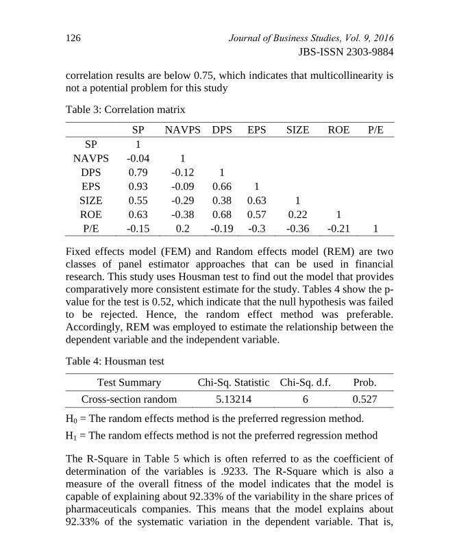
126 Journal of Business Studies, Vol. 9, 2016
JBS-ISSN 2303-9884
correlation results are below 0.75, which indicates that multicollinearity is
not a potential problem for this study
Table 3: Correlation matrix
SP NAVPS DPS EPS SIZE ROE P/E
SP 1
NAVPS -0.04 1
DPS 0.79 -0.12 1
EPS 0.93 -0.09 0.66 1
SIZE 0.55 -0.29 0.38 0.63 1
ROE 0.63 -0.38 0.68 0.57 0.22 1
P/E -0.15 0.2 -0.19 -0.3 -0.36 -0.21 1
Fixed effects model (FEM) and Random effects model (REM) are two
classes of panel estimator approaches that can be used in financial
research. This study uses Housman test to find out the model that provides
comparatively more consistent estimate for the study. Tables 4 show the p-
value for the test is 0.52, which indicate that the null hypothesis was failed
to be rejected. Hence, the random effect method was preferable.
Accordingly, REM was employed to estimate the relationship between the
dependent variable and the independent variable.
Table 4: Housman test
Test Summary Chi-Sq. Statistic Chi-Sq. d.f. Prob.
Cross-section random 5.13214 6 0.527
H0 = The random effects method is the preferred regression method.
H1 = The random effects method is not the preferred regression method
The R-Square in Table 5 which is often referred to as the coefficient of
determination of the variables is .9233. The R-Square which is also a
measure of the overall fitness of the model indicates that the model is
capable of explaining about 92.33% of the variability in the share prices of
pharmaceuticals companies. This means that the model explains about
92.33% of the systematic variation in the dependent variable. That is,

Journal of Business Studies, Vol. 9, 2016 127
JBS-ISSN 2303-9884
about 7.66% of the variations in market price of the sampled
pharmaceuticals companies are accounted for by other factors not captured
by the model. This result is complimented by the adjusted R- square of
about 91.37%, which in essence is the proportion of total variance that is
explained by the model.
The DW test statistic value in the multivariate regression result is 1.70.
According to DW stat. table, the relevant critical values for the test are
lower critical value(dL) = 1.172 and upper critical value(dU) = 1.638, so 4
− dU = 2.362 and 4 − dL = 2.828. The DW test statistic value is clearly
between 1.638 to 2.362. So, the null hypothesis is not rejected and no
significant residual autocorrelation was presumed. Similarly, findings
from the Fishers ratio (i.e., the F-Statistics) which is a proof of the validity
of the estimated model as reflected in Table 5, indicates that, the F is about
96.349 and a p-value or F(sig) that is equal to 0.000, this invariably
suggests clearly that simultaneously the explanatory variables are
significantly associated with the dependent variable. That is, they strongly
determine the behavior of the market values of share prices
Table 5: Regression result-REM
Variable Coefficient Std. Error t-Statistic Prob.
NAVPS 0.088677 0.039731 2.23193 0.0303
DPS 11.49781 1.777874 6.46717 0.0000
EPS 19.27831 1.421481 13.5621 0.0000
LN(SIZE) 17.22947 8.650343 1.99177 0.0521
ROE 283.7409 136.8093 2.07399 0.0435
P/E 2.287929 0.504109 4.53856 0.0000
C -452.7322 196.0555 -2.3092 0.0253
R-squared 0.923334
Adjusted R-squared 0.913751
F-statistic 96.34927
Prob(F-statistic) 0.00000
Durbin-Watson stat(DW) 1.705467
128 Journal of Business Studies, Vol. 9, 2016
JBS-ISSN 2303-9884
The model we estimated is given below:
SPit = β0 + β1NAVPSit + β2DPSit + β3EPSit + β4SIZEit P/Eit + β5ROEit +
β6 P/Eit + εit
Where,
Dependent variable, SP: Stock price
Independent variables, : NAVPS = Net asset value per share
DPS = Dividend per share
EPS = Earnings per share
SIZE = Firm size
ROE = Return on equity
P/E = Price earnings ratio
Table 5 shows that net asset value per share has a positive relationship
with share price. This result basically means that with the influence of
other variable held constant, firm’s net asset value per share will have
positive impact on market price. Empirical findings provided in the Table
5 show that there is a significant positive relationship between dividend
per share and share price of the listed pharmaceuticals companies in DSE.
This is evident in the t-statistics=6.46 with p value 0.000. However,
further empirical finding from the regression analysis shows a positive
relationship between EPS and share price. This is evident in the t-statistics
value of (t-statistics = 13.56and the p-value =.000). The results can be
explained as that an increase in earnings per share will invariably bring
about a significant increase in the market prices of equity shares. Another
empirical finding from the regression analysis shows that there is positive
relationship between P/E ratio and SP. The coefficient of P/E ratio is
2.287which mean that when there is 1-unit increase in price to earnings
ratio, the share prices will increase by BDT.2.287. Finally, variables
LN(SIZE) have significant impact on share price. This indicates that SIZE
have an explanatory power toward stock price movement.

Journal of Business Studies, Vol. 9, 2016 129
JBS-ISSN 2303-9884
(VI) Discussions of Major Findings
Net Asset Value Per Share(NAVPS)
This study showed that significant positive relationship between share
price and net asset value per share. The previous literature supports this
finding like the studies of Sharma (2011) Arshad et al. (2015), Uddin et al.
(2013) and Almumani (2014). The reason behind positive relationship
between net asset value per share and share price is that book value per
share is the owner’s funds, a higher book value per share is perhaps
perceived by an investor to be an indicator of the sound financial position
of a company for investing.
Dividend Per Share (DPS)
This model showed that there is positive association between dividend per
share and share price. This result is consistent with results of Zahir and
Khanna (1982), Balkrishan (1984), Malhotra (1987) that dividend per
share has positive and significant impact on market price of share.
Earnings Per Share (EPS)
Significant positive relationship between earning per share and stock price
has been found in the statistical test. It can be explained that when earning
per share increase, it will boost up company’s share price. The present
study tends to support the viewpoints of Sharma (2011), Arshad et al.
(2015), Uddin et al. (2013, and Almumani (2014), Zahir and Khanna
(1982), Balkrishan (1984), Malhotra (1987).
Firm Size (SIZE)
Firm size was used in this study in terms of market capitalization of a
firm. This study showed that relationship between firm size and share
price are statistically being significant. These finding is consistent with
previous researcher’s findings that the firm size is having significant
positive relationship with stock price. Srinivasan (2012) found that
positive relationship exists between stock price and firm size. Chandra
(1981) also found that size has significant positive impact on market price
of share.
130 Journal of Business Studies, Vol. 9, 2016
JBS-ISSN 2303-9884
Return on Equity(ROE)
Profitability of a firm greatly influences the market share price. In this
study, return on equity is used as proxy of profitability of firm. Results
show statistically significant positive relationship between return on equity
and share price. This finding is consistent with the findings of Chandra
(1981) that returns have a positive influence on share price.
Price Earnings Ratio(P/E)
Empirical findings from the regression analysis shows positive linear
relationship between price earnings ratio and share price. This outcome is
supported by Uddin et al. (2013), Almumani (2014), and Bhattarai (2014)
that has a significant positive relation exists between price earnings ratio
and share price.
(VII) Conclusion
This study examines the relationship between the selected variables (net asset value per share, dividend per share, earnings per share, firm size, return on equity and price earnings ratio) and the stock price in DSE, by means of panel data techniques (REM)for the period from 2010 to 2014. The conclusion drawn from this study is that a significant relationship exists between the DSE stock prices and all the selected microeconomic variables. Specifically, the study found that net asset value per share, dividend per share, earnings per share, firm size, return on equity, price earnings ratio are positively affecting the stock price. The result of this study has similarities with the result of the previous studies. Like, the study result of Arshad et al. (2015), Uddin et al. (2013, and Almumani (2014), Zahir and Khanna (1982), Balkrishan (1984) and Malhotra (1987), this study also revealed that share price has positive relations with net asset value per share, earnings per share, firm size, return on equity and price earnings ratio. This study has a lot of implications to the managers and the investors. The findings of this study will help managers knowing the factors that affect share price and the factors that needed to be emphasized to maximize share price. Besides, the investors can take their investment decision on the basis of this result. Despite having important implications, this paper also has limitations. This paper is done using the pharmaceuticals sector data only. So, it might not be applicable to the other sector. Future studies need to be done on the determinants of share price including all the industries enlisted in DSE.
Journal of Business Studies, Vol. 9, 2016 131
JBS-ISSN 2303-9884
References
Almumani, M. A. (2014), “Determinants of equity share prices of the
listed banks in Amman stock exchange: Quantitative approach”,
International Journal of Business and Social Science, Vol. 5, pp.
91-104.
Arshad, Z., Arshaad, A. R., Yousaf, S., & Jamil, S. (2015), “Determinants
of Share Prices of listed Commercial Banks in Pakistan”,Journal of
Economics and Finance, Vol. 6, pp.56-64.
Balakrishnan (1984), “Determinants of Equity Prices in India”,
Management Accountant, Vol.19, pp. 728-730.
Bhattarai, Y. R. (2014), “Determinants of Share Price of Nepalese
Commercial Banks”,Economic Journal of Development Issues,
Vol. 17, pp. 187-197.
Chandra, P. (1981), “Valuation of equity shares in India”,New Delhi:
Sultan Chand and Sons.
Jatoi, M.Z., Shabir, G.,Hamad, N.,Iqbal N. & Muhammad, K. (2014), “A
Regressional impact of earning per share on market value of share:
A case study cement industry of Pakistan”,International Journal
of Academic Research in Accounting, Finance and Management
Sciences,Vol.4, pp. 221-227.
Hausman J.A (1978), “Specification Tests in Econometrics”,
Econometrica, Vol. 46, pp. 1251- 1271.
Iqbal , A., Ahmed , F., & Zaidi, S. S. (2015),“Determinants of Share
Prices, Evidence from Oil & Gas and Cement Sector of Karachi
Stock Exchange (A Panel Data Approach)”,Journal of Poverty,
Investment and Development, Vol.8, pp. 14-19.
Keynes, John Maynard (1936), The General Theory of Employment,
Interest and Money, New York: Harcourt Brace and Co.
Malhotra N. K.(2007),Basic Marketing Reserach :A Decesion-Making
Apporach, New jersey: Person Education, Inc.

132 Journal of Business Studies, Vol. 9, 2016
JBS-ISSN 2303-9884
Malhotra, N., &Tandon, K. (2013), “Determinants of stock prices:
Empirical evidence from NSE 100 companies”, International
Journal of Research in Management &Technology, Vol.3, pp. 86-
95.
Malik , F. M., Quresh, M. U., & Azeem , M. (2012), “ Determination of
Share Price: Evidence from Karachi Stock Exchange”, The
Romanian Economic Journal, Vol. 4, pp. 97-114.
Ohlson, J. (1995), “Earnings, Book values and Dividends in Equity
valuation”, Contemporary Accounting Research, Vol. 11, pp. 661
– 687.
Sharma, S. (2011), “Determinants of equity share prices in India”, Journal
of Arts, Science & Commerce, Vol. 2, pp. 51-60.
Sharpe, William F. (1964), “Capital asset prices: A theory of market
equilibrium under conditions of risk”, Journal of Finance, Vol.19,
pp. 425–442.
Srinivasan, P. (2012), “Determinants of equity share prices in India: A
panel data approach”, The Romanian Economic Journal, Vol. 46,
pp. 205-228.
Uddin, M. R., Rahman, S. Z., & Hossain , M. R. (2013), “ Determinants of
Stock Prices in Financial Sector Companies in Bangladesh- A
Study on Dhaka Stock Exchange (DSE)”,Interdisciplinary Journal
of Contemporary Research in Business, Vol 5, pp. 471-477.
Zahir, M., & Khanna, Y. (1982), “Determinants of stock prices in India”,
The Chartered Accountant, Vol. 30, pp. 521-523.

Journal of Business Studies, Vol. 9, 2016 133
JBS-ISSN 2303-9884
Influence of Cognitive and Affective Image on a Recreational
Park: An Empirical Study
Md. Ikbal Hossain 1
Rebeka Sultana Rekha 2
Dr. Md. Enayet Hossain 3
Abstract
This empirical study is conducted to test the influence of cognitive and affective
image on a recreational Park at Rajshahi in Bangladesh. In total 257 samples are
collected from the visitors at the destination using seven Point Likert-Scale.
Initially an exploratory factor analysis is employed and regression analysis is
performed to test the individual relationship of factor with the cognitive and
affective images using SPSS 15.00. The main outcome of the analysis present
total six cognitive (Entertainment & Recreation Facilities, Food & Beverage
Facilities, Transportation & Safety Facilities, Infrastructure, Price Charges and
Natural & Artificial Environment) and two affective (Pleasant & Relaxing)
influential factors which have significant relationship with cognitive and
affective images. Thus, the eight hypotheses are accepted which will enrich the
existing literatures. The park operator will get insight knowledge for developing
image of the destination. Theoretical implications are discussed including
limitation and future research direction.
Keywords: Cognitive image, affective image, factor analysis, regression analysis
(I) Introduction
oday’s tourism market is very much competitive and should revise to
attract visitors where an image of a destination is the most important
issue. Destination image is described as simply impressions of a place or
perceptions of an area (Echtner & Ritchie 2003). It is also the concept of
expression of all objective knowledge, prejudices, imagination and
emotional thoughts of an individual or group about a particular location
1 Assistant Professor, Department of Marketing, University of Rajshahi,
Email: [email protected] 2 Lecturer, Department of Business Administration, Pabna University of Science and
Technology, Email: [email protected] 3 Professor, Department of Marketing, University of Rajshahi,
Email: [email protected]
T

134 Journal of Business Studies, Vol. 9, 2016
JBS-ISSN 2303-9884
(Lawson & Baud (1977). It is a multidimensional constructs comprising of
several primary dimensions (Ahmed 1996; Baloglu & McCleary 1999;
Echtner & Ritchie 1993; Lawson & Baud 1977; Leisen 2001) which is the
growing interest for researchers of the day.
Cognitive and affective are the two major perspectives of analyzing the
image of a destination (Lawson & Baud, 1977). The cognitive image’s is
known as perceptual component which can be interpreted as the whole
beliefs and knowledge about the physical attributes of a destination. The
affective image’s refers to the appraisal of the affective quality of feelings
towards the attributes and the surrounding environments (Baloglu &
McCleary, 1999). The authors also suggest that destination image as the
sum of the perception of cognitive evaluation based on information
sources and age, and affective ones influenced by socio-psychological and
demographical factors. Leisen (2001) states that affective associations
greatly influence the image, an individual has of a destination and
therefore, destination choice. So, destination image has significant effect
on the development of the destination through satisfying visitors, to retain
them and for developing the tourism sector of a country.
Though, tourism sector of Bangladesh is one of the fastest growing sectors
which needs to revise its image for attracting and satisfying visitors, yet
foreign visitors arrival expanded from 207,199 in 2001 to 303,386 visitors
in 2010 (Bangladesh Parjatan Corporation). The growth indicates light of
further scope by maximizing use of existing resources (Islam &
Nuruzzaman 2009). There are seven divisions and 64 districts in
Bangladesh which refer unique tourism flavor individually. The study is
conducted at Rajshahi district which contains more than 20 tourism spots
(such as Zia Park, Central Zoo, Veranda Museum(1st Museum in
Bangladesh), Padma Garden, T-Damp, Sericulture, University of Rajshahi,
Vadra Park, Putia Rajbari and River Bank etc.). Most of the visitors often
visit Zia Park, Central Zoo, Putia Rajbari, Veranda Museum and Padma
Garden (on the bank of River Padma). This empirical study is mainly
focused on Zia Recreational Park to understand the factors and its
relationship with cognitive and affective images.

Journal of Business Studies, Vol. 9, 2016 135
JBS-ISSN 2303-9884
(II) An overview of the Recreational Park
Bell, Tyrvainen, Seivanen, Probstl, and Simpson (2007) find that recreation is the activities of people in the nature as the part of their leisure
time. Recreation Park is developed by state to maximize social welfare of
people and for their recreation (Pauta & Siavanen, 2001). This recreational
park is situated in city of education (Rajshahi) in Bangladesh which was
also the special project of the People’s Republic of Bangladesh. Domestic
Engineering & Technology Services (DETS) constructs the park within
the contractual time (2 years) and also get the management authority for
ten years from Rajshahi City Corporation. They get the authority by
making contact of sharing income under the supervision of this city
corporation. This park is situated on 12.21 acres land which has 18
different paid & few non-paid rides for children and adult people (Hossain
& Hossain, 2014). It has been opened to general people on 25th
, February
2006. It is the most attractive and well furnished park in the northern zone
in Bangladesh and opened to visitors from 10.00 am to 8.00 pm in the
whole year. The peak session for the park is from August to February and
most of the visitors come from different educational institutions (schools
and colleges) for education tour, picnic parties from different places, local
picnic parties and the residential people. Hossain and Hossain (2014) also
depict more than 1.2 lakh visitor visit this destination over the year which
also plays an important role for economic contribution and for
employment opportunity in the northern region. This park provides Tk.
35.70 lakh (1$ = 78.00 Taka) respectively to the Rajshahi City
Corporation in 2011 and 2012. There are 82 people employed to conduct
the park activities smoothly. Moreover, many local people are directly and
indirectly dependent on this park for their earnings and livings by
conducting different business activities (Shops, Restaurants, Tea stall and
Transportation services etc.).
(III) Brief Literature Review
Image and Destination Image
Beerli and Martin (2004) depict that an image is seen as a mental picture
formed by a set of attributes that defines the destination in its various
dimension, influences destination selection process. They further suggest a
destination image can be created from an individual’s general knowledge

136 Journal of Business Studies, Vol. 9, 2016
JBS-ISSN 2303-9884
or feelings, external influence from friends and relatives, advertisements
and their own past experience. On the other hand, Milman and Pizam
(1995) suggest that destination image consists of three main components;
firstly, the product, for example the quality of attraction, the attitude of the
destination hosts and the environment; secondly the weather or climate
and lastly the facilities available in the destination. Destination managers
or organizations need to consider all three components with equal
importance to retain tourist’s confidence on their products and to influence
their behavior. Beside these, destination image plays two important roles
in behaviors: (1) to influence the destination choice decision-making
process and (2) to condition the after-decision-making behaviors including
participation (on-site experience), evaluation (satisfaction) and future
behavioral intentions (intention to revisit and willingness to recommend)
(Ashworth & Goodall, 1988; Bigne, Sanchez & Sanchez, 2001; Cooper,
Fletcher, Gilbert & Wanhill, 1993; Lee, Lee, & Lee, 2005; Mansfeld,
1992). Moreover, cognitive image have a direct influence a destination
and represent its overall image (Beeril & Martin, 2004).
Therefore, destination image is a view of picture that attracts the visitors
to the destination and makes them spend much more money there. At the
same time, image views different things for different people (White, 2005)
and destination image is the beliefs, thought and impression of a tourist
about a place and the picture in their minds relating to that place (Watkins,
Hassanien & Dale 2006). Beside these, the image of a place is an
important asset (Ryan & Gu 2008). They further emphasize that image
itself is the beginning point of tourists expectation to visit the destination.
Unfortunately, most the image studies only considers cognitive image to
analyze the image of a destination. This study considers both cognitive
and affective components to analyze their influence on the destination
which is also considered in many recent image studies to measure the
overall image in different cultures’ (Baloglu & McCleary, 1999; Beerli &
Martin, 2004; Hosany, Ekinci, & Uysal, 2007; Lee et al., 2005; Martin &
Bosque, 2008; Phillips & Jang, 2008).
Cognitive Image
Cognitive image refers to beliefs and knowledge about an object or place
(Baloglu & Brinberg 1997; Gartner 1993; Walmsley & Jenkins, 1993). It
Journal of Business Studies, Vol. 9, 2016 137
JBS-ISSN 2303-9884
is also described as the beliefs and information that visitors have about a
place (Coban, 2012). Cognitive image is directly observable, descriptive
and measurable which may provide more concrete and interpretive
information regarding the uniqueness of a destination (Walmsley &
Young, 1998). It comprises objective reality of destination attributes
(Tasci & Gartne, 2007). Numerous studies are conducted by researchers to
measure the destination image considering only the cognitive image
(Chen, 2001; Chen & Kerstetter, 1999; Leisen, 2001) and different studies
consider different dimensions (Liu, Lin & Wang, 2012). This study
considers six cognitive factors (Entertainment & recreation, Food &
beverage, Infrastructure, Transportation & security, Price charges and
Natural Environment) which are common to different image studies and
contain variables (table 1).
First, entertainment and recreation facilities are one the most attractive
factor which visitors consider to choice and select a destination for
visiting. Though, this study is conducted on a park, it appears very
important to represent the cognitive image of the destination. Then, the
hypothesis is drowned as follow-
Hypothesis 1: The factor entertainment and recreation facilities positively
influence the cognitive image of the destination.
Second, food and beverage is also important to visitors for visiting a
destination. Usually, visitors spend much time there and they need launch
and snacks etc. If a destination can ensure the availability of quality
restaurants, food corners etc; it can attract more visitors. So, it appears
significant to weight the cognitive image of the destination and the
hypothesis is
Hypothesis 2: The factor food and beverage facilities positively influence
the cognitive image of the destination.
Third, infrastructure plays also key role to attract visitors towards a
destination. This study also considers this important factor and proposes
hypothesis to test its’ relationship with cognitive image of the destination.
The hypothesis is in below-
138 Journal of Business Studies, Vol. 9, 2016
JBS-ISSN 2303-9884
Hypothesis 3: The factor infrastructure positively influences the cognitive
image of the destination.
Fourth, transportation facilities are also an important indicator to easily
access a destination and safety is important for physical and mental relieve
of visitors. This study considers this factor and tries to test its influence on
cognitive image of the destination. The drawing hypothesis is-
Hypothesis 4: The factor transportation and safety facilities positively
influence the cognitive image of the destination.
Fifth, Price plays an important role to visit or not to visit a destination
and the most successful destination always offers competitive price for its
different offerings to attract more visitors. This study considers it as factor
and the hypothesis is drawing as-
Hypothesis 5: The factor price charges positively influence the cognitive
image of the destination.
Sixth, natural environment is very much important for the mental pleasure
of visitors towards a destination for visiting. Because, they normally visit
a destination with family, friends and relatives etc and this factor plays an
important role to taking final visiting decision to visitors. The study
considers this important factor and is drowned the hypothesis to test its
influence on cognitive image as follow-
Hypothesis 6: The factor natural environment positively influence the
cognitive image of the destination.
Affective Image
Baloglu and McCleary (1999) depict that affective image is the emotional
feelings about the destination attributes and surroundings environment. It
is the evaluation of visitors towards a destination and the evaluation may
be positive or negative (Woodside & Lysonki, 1989). Many studies
consider affective image component with cognitive image to measure the
destination image. This study considers two factors (pleasant place to visit
and relaxing place to visit) which are used in different study also to
measure the affective image (table 1).

Journal of Business Studies, Vol. 9, 2016 139
JBS-ISSN 2303-9884
First, the factor pleasant place to visit the park is considered as an
important affective issue. Normally, visitors visit those destinations which
seem pleasant to them. Later on, they take their final decision for visiting
and evaluate the destination on this regard. So, this study considers it and
tries to test its relationship with affective image and the proposed
hypothesis is-
Hypothesis 7: The factor pleasant place to visit positively influences the
affective image of the destination.
Second, the factor relaxing place to visit is also important to visitors. If
they think the destination is free of risk (mentally and physically). If they
can visit with relaxation, it increases more visitors for visiting the
destination. This study considers this important factor for study and the
proposed hypothesis is-
Hypothesis 8: The factor relaxing place to visit positively influences the
affective image of the destination.
This study treats both the cognitive and affective image components
independently by considering its attributes in understanding the image of
the destination which is not seen in previous image studies. Then, it
considers testing the influence of eight factors individually to measure
their relationship with cognitive and affective images. This study has also
been carried out in tourism sector and Zia Park has been chosen as the
study context. The reason of choosing the destination is that there are not
available literatures on this park. But it is the most attractive, amusement
and recreational places not only in Rajshahi city but also in the northern
zone in Bangladesh. Many domestic visitors visit this destination each
year. So, the study is conducted to understand the park image and to look
for main reasons behinds for visiting this destination. To fill up the gaps,
the present study conducts to explore the variables and factors of cognitive
and affective image of the park. In addition to that it also explores the
attributes of cognitive and affective images. Finally, it tests the
relationship of factors with independent cognitive and affective image of
the destination.
140 Journal of Business Studies, Vol. 9, 2016
JBS-ISSN 2303-9884
(IV) Research Methodology
Sampling and Data Collection
The study considers quantitative method to collect data which is very
much popular in marketing and social science research. This method is
used for three purposes, First, it reflect the post- positivist philosophical
assumption; Second, it allows simple statistical tools, easy to administrate,
code the data for further processing and resulting in easy writing; Third,
statistically organized image analysis is helpful to compare with other
destinations which might be of interest of the destination operators or
managers. While the study considered the spot visitors as target
populations and the sample size are 257 by considering the convenient
sampling method due to the convenience and availability of the
respondents (Babble, 1990). A total of 350 questionnaires were distributed
and 302 questionnaires were returned, representing a response rate of
86.28%. After screening of completeness of the questionnaires, 257
samples were deemed to final analysis.
Survey Questionnaire Design
The questionnaire was developed based on existing literature which was
tested empirically in previous study (Hossain & Hossain, 2014). It
contained three sections. The first section contained the 34 variables and
10 attributes of cognitive image. The second section contained 10
variables and 2 attributes of affective image of the park. Likert-Scale was
used to indicate the level of agreement of the respondents ranging from 7
= very strongly agree and 1= very strongly disagree for both sections. This
scale is very much popular and widely used to understand and measure
perception, evaluation, beliefs and attitude of customers or visitors toward
an object, brand, place and product (Malhotra, Hall, Shaw, & Crisp, 1996).
This scale also provides more accurate data than 5- point Liker-Scale for
statistical analysis. Secondary sources were used to generate variables and
attributes for both of these sections also. It included brochures, paper
cutting and promotional materials about the destination and review of park
and tourism destination related literatures that focus on destination image,
perceived image, tourists/ visitors attraction, attitude, satisfaction and
cognition (Aksoy 2011; Beerli & Martín 2004; Hossain & Hossain, 2014;
Liu, Liu, Huang & Wen 2010). The last section of the questionnaire was
Journal of Business Studies, Vol. 9, 2016 141
JBS-ISSN 2303-9884
related to the socio-demographic information of the respondents to
identify their characteristics. Moreover, there are two questions included
to determine the respondents’ intention to revisit the Park using
dichotomous-scale and for the number of visited time using ordinal-scale.
These scales are also widely used in social science research.
Pilot Test
This empirical study also conducted a pilot test to ensure its clarity,
reliability and comprehensiveness of the questionnaire and thirty (30)
questionnaires were distributed to 25 MBA students and 5 faculty
members (Department of Marketing, University of Rajshahi, Bangladesh)
who were visited the Park at least once. Some modifications to the
wording are made on the basis of recommendation of pilot test.
Scale reliability
A reliability analysis (Cronbach’s Alpha) is used to gauge the reliability of
the instrument’s items which determines the internal consistency or
average correlation of the items. The reliability analysis reveals that the
alpha coefficient is 0.913 for cognitive and 0.852 for affective images,
which exceeds the minimum coefficient (0.5) suggests by Hair, Anderson,
Tatham and Black (1998).
Data analysis
The data are analyzed using the Statistical Package for the Social Sciences
(SPSS 15). Descriptive statistics are used to analyze the distribution of the
data. An exploratory factor analysis is performed to reduce the number of
items to a few correlated dimensions. It has been used to explore the
possible underlying factor structure of a set of observed variables without
imposing a preconceived structure on the outcome (Child, 1990). The
Principal Components and Orthogonal (VARIMAX) rotation methodology
is used and only factors with Eigen value equal or greater than one (1) are
retained. A variable with a factor loading of 0.5 or more is kept in a factor.
Finally, regression analysis is performed where dependent variables are
cognitive and affective images and independent variables are the attained
exploratory factors of the destination. Then, two regression models are
developed for these two images (Cognitive Affective) to test the
142 Journal of Business Studies, Vol. 9, 2016
JBS-ISSN 2303-9884
relationship of 8 factors with these images statistically which are given in
below-
1) The regression models for the cognitive image of the Zia Park is-
)1( ............................2101 eXXY nn
Where,
= Dependent Variable: Cognitive Image
= Regression of coefficient intercept
=Regression coefficient of independent variables
= Independent variables (Entertainment & recreation, Food &
beverage, Transportation & Safety, Infrastructure, Price charges
and Natural environment)
e = Random error
2) The regression models for the affective image of the Zia Park is-
(2) ..................221102 eXXXY nn
Where,
Y2 = Dependent Variable: Affective Image
β0 = Regression of coefficient intercept
βn Xn = Regression coefficient of independent variables
X1X2= Independent variables (Pleasant place and Relaxing
place)
e = Random error
(V) Results and Discussions
Profile of Respondents
The useable questionnaires are distributed to 257 respondents,
representing 65.4% male and 34.6% female respectively. Near half of the
respondents are in the age group of 21-30 years, representing 49.4% and
younger than 20 years of age is the second largest portion representing
21.8% of the respondents. Most of the respondents’ professional
background includes students 49%, government employees 16.7% and
private organization employees 17.5%. In addition, the survey reveals that
Journal of Business Studies, Vol. 9, 2016 143
JBS-ISSN 2303-9884
the education level of visitors to Zia Park is relatively high, with 45.9%
completed graduation degrees. While 19.8% of the respondents complete
higher secondary certificate education and only 14.8% of the respondents
complete their secondary school certificate education. With regards to
personal monthly income measures in taka, the study reveals that 28.8% of
the visitors report their or their parents’ monthly income in the range
between 10,000Tk to 20,000Tk and 22.6% of the respondents earn less
than 10,000Tk. It denotes that most of the visitors fall in lower level
income group. While 54.5% of the respondents are single and 45.5% are
married respectively. A majority of respondents 81.3% are from the
Rajshahi division which indicates that most of the visitors are local people.
At the same time as, 7.4% of the respondents are from the Dhaka division
and 4.3% are from Khulna division. Whereas over half, 50.2% of
respondents visit this place more than 5 times and 32.7% of the
respondents are 2 to 5 times. Only 17.1 % of the respondents are the first
time visitors at this Park. While 87.2% respondents want to visit this park
again and 10.5 % respondents are in under-consideration (Table 2)
Cognitive image dimension
The results of Bartlett test of Sphericity is significant (x² =3154.055, p =
0.000). The overall value of the Kaiser-Meyer-Olkin overall measure of
sampling adequacy (MSA) is 0.894, which is well above the
recommended threshold of sampling adequacy at the minimum of 0.5
(Hair et al., 1998). These two tests suggest that the data is suitable for
exploratory factor analysis. Base on the Eigen value greater than one,
scree-plot criteria and the percentage of variance criterion, six factors (6)
are retained which capture 64.39% of the total variance. Among the 34
cognitive image attributes, eight has factor loading less than .50. These are
“Availability of mobile network,” “Dustbin facilities,” “Train
transportation facilities,” “Rides ticket price,” “Various trees available at
the park”, “Prayer facilities”, “Free entering facilities” and
“Toilet/washroom facilities”. These are evaluated for possible deletion
following by the criterion of Hair et al. (1998). The dropping of these
variables with low factor loading the total variance explanation increases
more than 3% (from 61.02% to 64.39%). The results of the principle
component analysis with orthogonal (VARIMAX) rotations are shown in
144 Journal of Business Studies, Vol. 9, 2016
JBS-ISSN 2303-9884
Table 3. The scale reliability for each factor is tested also for internal
consistency by assessing the item –to-total correlation for each separate
item and Cronbach’s alpha is considered for the consistency of the entire
scale. The rules of thumb suggest that item-to-total correlations exceed .50
and lower limit for Cronbach’s alpha value is .67. The result shows that
the alpha coefficient ranges from .67 to .87 for the six factors (Table 3).
Factors are labeled based on highly loaded items and the common
characteristics of the items they include. They are labeled as
“Entertainment & recreation facilities”, (Factor 1), “Food & beverage
facilities,” (Factor 2). “Transportation and safety facilities”, (Factor 3),
“Infrastructure”, (Factor 4), “Price charges”, (Factor 5), and “Natural &
artificial environment”, (Factor 6). While cognitive image is the result of
the mean value of 10 cognitive attributes. These include the overall belief
of the respondents about rides facility, environmental scenery, safety &
security, food, entertainment & recreation, structure & location, facility
services, management services, price charges and transportation facility).
Where the environmental scenery shows the highest mean value (5.53)
and price charges shows the lowest one (4.36). While, others bear the near
or same value which indicate the respondents’ cognitive image towards
the recreational park is very positive.
In addition, regression analysis is performed to examine the relationship of
six (6) factors with cognitive image of the park taking a 5% significance
level. The regression equation characteristics of cognitive image indicates
a good adjusted R² =0.708 (Table 5). T his indicates that more than 70%
of the variation is explained by the equation where the F-ratio of 100.990
is significant. The regression analysis shows that the cognitive image has
statistically significant beta coefficients (p.000). So, there are a positive
relationship between the independent variables and the dependent
variable.
The factor (entertainment & recreation facilities) shows the result
(Standardized, β=0.126, t = 2.631) which indicates the positive
relationship with the cognitive image. Thus, the first hypothesis is
accepted. While the average value of this factor’s variables are not so high
which indicate the facilities unavailability or poor quality to visitors. The
park operator should give more attention to improve the quality and make

Journal of Business Studies, Vol. 9, 2016 145
JBS-ISSN 2303-9884
more noticeable these facilities to develop image and to attract more
visitors. While, factor (food & beverage facilities) shows the regression
results (Standardized, β=0.221, t = 4.595) which denote its positive
relationship with cognitive image. Thus, the second hypothesis is also
accepted. The destination authority or manager should ensure more quality
restaurants and food corners to make available the fast foods and
preferable foods to visitors which indicate the lowest opinion of studies
from the descriptive study.
In addition to, the factor transportation & safety facilities shows the
regression result (Standardized, β=0.433, t = 9.954) which mean the
positive relationship with cognitive image and the hypothesis is accepted.
The facilities within this factor are available to visitors and the destination
should continue it to improve its image. On the other hand, the factor
(infrastructure) shows the results (Standardized, β=0.090, t = 2.005) which
indicate its positive relationship with cognitive image and the fourth
hypothesis is accepted also. It can be recommended from the descriptive
studies that the authority should revise the facilities within this factor
specialty to enlarge the area of the park.
Furthermore, price charges shows the results (Standardized, β=0.143, t =
3.325) which also indicate its positive relationship with the cognitive
image and the hypothesis is accepted. But the descriptive study of this
factor does not show satisfactory result especially to the variable price
charges for buying different goods at the park. The authority or manager
of the park should revise their offerings price and set up competitive price
to develop the park image and attract more visitors. Because most of the
visitors are in lower level income group and residence people and they are
very much price sensitive. Moreover, the factor natural and artificial
environment show the regression results (Standardized, β=0.221, t =
4.595) which show the positive relationship with the cognitive image and
the hypothesis is accepted. The descriptive results of the variables within
this factors show the highest opinion of visitors which indicate the
availability of the facilities in the destination. The operator should
continue these facilities and make more visible to develop the park
cognitive image. The regression model for the cognitive image of the park
is described in below-
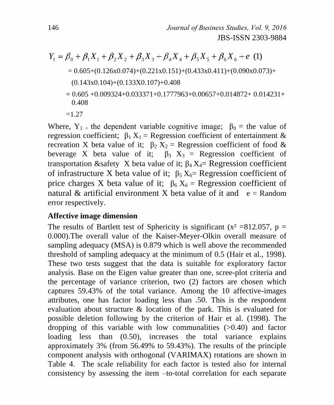
146 Journal of Business Studies, Vol. 9, 2016
JBS-ISSN 2303-9884
)1( 66554433221101 eXXXXXXY
= 0.605+(0.126x0.074)+(0.221x0.151)+(0.433x0.411)+(0.090x0.073)+
(0.143x0.104)+(0.133X0.107)+0.408
= 0.605 +0.009324+0.033371+0.1777963+0.00657+0.014872+ 0.014231+
0.408
=1.27
Where, Y1 = the dependent variable cognitive image; β0 = the value of
regression coefficient; β1 X1 = Regression coefficient of entertainment &
recreation X beta value of it; β2 X2 = Regression coefficient of food &
beverage X beta value of it; β3 X3 = Regression coefficient of
transportation &safety X beta value of it; β4 X4= Regression coefficient
of infrastructure X beta value of it; β5 X6= Regression coefficient of
price charges X beta value of it; β6 X6 = Regression coefficient of
natural & artificial environment X beta value of it and e = Random
error respectively.
Affective image dimension
The results of Bartlett test of Sphericity is significant (x² =812.057, p =
0.000).The overall value of the Kaiser-Meyer-Olkin overall measure of
sampling adequacy (MSA) is 0.879 which is well above the recommended
threshold of sampling adequacy at the minimum of 0.5 (Hair et al., 1998).
These two tests suggest that the data is suitable for exploratory factor
analysis. Base on the Eigen value greater than one, scree-plot criteria and
the percentage of variance criterion, two (2) factors are chosen which
captures 59.43% of the total variance. Among the 10 affective-images
attributes, one has factor loading less than .50. This is the respondent
evaluation about structure & location of the park. This is evaluated for
possible deletion following by the criterion of Hair et al. (1998). The
dropping of this variable with low communalities (>0.40) and factor
loading less than (0.50), increases the total variance explains
approximately 3% (from 56.49% to 59.43%). The results of the principle
component analysis with orthogonal (VARIMAX) rotations are shown in
Table 4. The scale reliability for each factor is tested also for internal
consistency by assessing the item –to-total correlation for each separate
Journal of Business Studies, Vol. 9, 2016 147
JBS-ISSN 2303-9884
item and Cronbach’s alpha for the consistency of the entire scale. The
rules of thumb suggest that item-to-total correlations exceed .50 and lower
limit for Cronbach’s alpha value is 0.773. The result shows that the alpha
coefficient ranges from 0.773 to 0.799 for the two factors. Factors are
labeled based on highly loaded items and the common characteristics of
the items they include. They are labeled as “Pleasant place to visit”,
(Factor 1) and “Relaxing place to visit,” (Factor 2). The first factor
explains of the variance 47.19% and it bears Cronbach’s alpha coefficient
0.799. The second factor explains of the variance 12.23% and it bears
Cronbach’s alpha coefficient 0.773. So, both of the factors have high inner
consistency and scale reliability. While affective image is the result of the
mean value of 2 affective attributes. These include the visitors feeling
about the recreational park as pleasant and relaxation. The attribute
(pleasant) shows the highest opinion (5.42) of the visitors and relaxation
shows the lowest one (5.34). It indicates the respondents’ affective image
towards the recreational park is very positive.
Similarly the cognitive image, the regression equation characteristics of
affective image indicates a good adjusted R² =0.887 (Table 6). This
indicates that near about 89% of the variation is explained by the equation
where the F-ratio of 1001.171 is significant. The regression analysis shows
that the affective image has statistically significant beta coefficients
(p.000). So, there are a positive relationship between these independent
variables and the dependent variable.
The independent variable (pleasant place to visit) show the results
(Standardized, β=0.542, t = 25.723) which indicates the positive
relationship of this factor with the affective image of the destination and
the proposed hypothesis is accepted. The descriptive study results show
that the visitors’ evaluation regarding the variables (price and food &
beverage) are not satisfactory. So, the park authority should give keen
attention in this regard to make the destination more pleasant among
visitors. The second factor of affective image is relaxing place to visit
and shows the results (Standardized, β=0.771, t = 36.615). These results
indicate that there is a positive relationship between the factor and
affective image of the destination. Thus, the hypothesis is accepted and
the respondents feel relax to visit this destination. The authority should
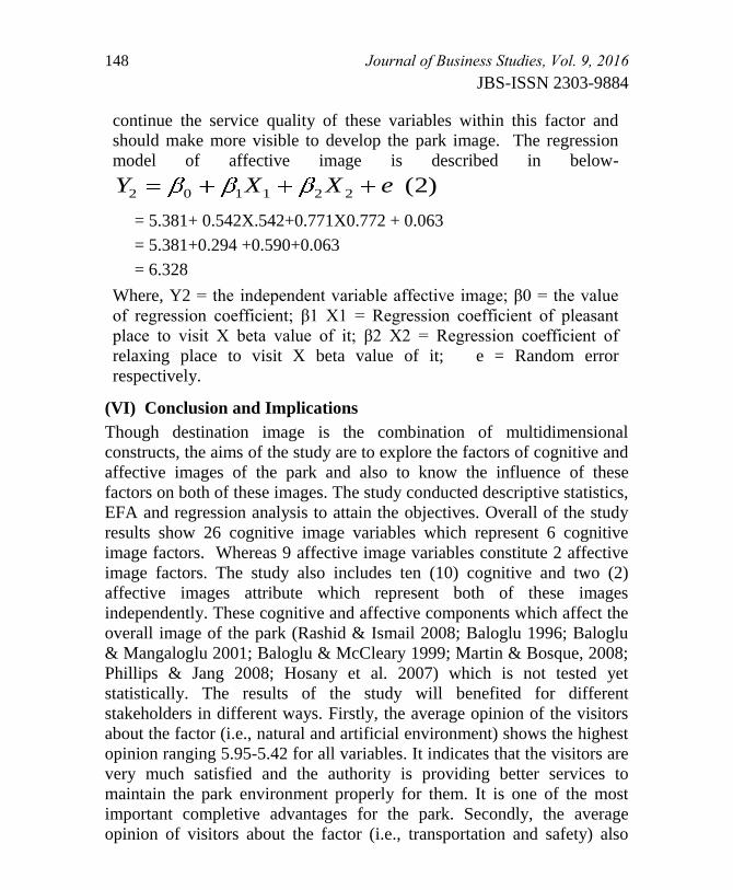
148 Journal of Business Studies, Vol. 9, 2016
JBS-ISSN 2303-9884
continue the service quality of these variables within this factor and
should make more visible to develop the park image. The regression
model of affective image is described in below-
)2( 221102 eXXY
= 5.381+ 0.542X.542+0.771X0.772 + 0.063
= 5.381+0.294 +0.590+0.063
= 6.328
Where, Y2 = the independent variable affective image; β0 = the value
of regression coefficient; β1 X1 = Regression coefficient of pleasant
place to visit X beta value of it; β2 X2 = Regression coefficient of
relaxing place to visit X beta value of it; e = Random error
respectively.
(VI) Conclusion and Implications
Though destination image is the combination of multidimensional
constructs, the aims of the study are to explore the factors of cognitive and
affective images of the park and also to know the influence of these
factors on both of these images. The study conducted descriptive statistics,
EFA and regression analysis to attain the objectives. Overall of the study
results show 26 cognitive image variables which represent 6 cognitive
image factors. Whereas 9 affective image variables constitute 2 affective
image factors. The study also includes ten (10) cognitive and two (2)
affective images attribute which represent both of these images
independently. These cognitive and affective components which affect the
overall image of the park (Rashid & Ismail 2008; Baloglu 1996; Baloglu
& Mangaloglu 2001; Baloglu & McCleary 1999; Martin & Bosque, 2008;
Phillips & Jang 2008; Hosany et al. 2007) which is not tested yet
statistically. The results of the study will benefited for different
stakeholders in different ways. Firstly, the average opinion of the visitors
about the factor (i.e., natural and artificial environment) shows the highest
opinion ranging 5.95-5.42 for all variables. It indicates that the visitors are
very much satisfied and the authority is providing better services to
maintain the park environment properly for them. It is one of the most
important completive advantages for the park. Secondly, the average
opinion of visitors about the factor (i.e., transportation and safety) also
Journal of Business Studies, Vol. 9, 2016 149
JBS-ISSN 2303-9884
shows moderately high opinion for all variables ranging 5.41-5.03 which
indicate the visitors feel safe and can easily access the park. It is also an
important strength for the park to attract more visitors. Thirdly, this study
elucidates different information for the visitors and authority relating to
the factors (i.e., entertainment & recreation and price charges) and all the
variables within these factors are not up to the mark. It ranges 4.02-3.35
for entertainment and recreation facilities available at the park which
indicates the number of different events should increase to satisfy and
attract more customers which will ultimately increase the image of this
park. The visitors opinion also express that the price for different services
at the park are not reasonable and it ranges 4.43-3.60 for the variables
within this factor. Though lower level income group people are interested
to visit this park, the authority should be rationale to charge for different
services at the park. In last but not for the least, the study indicates that all
the factors within cognitive image and affective image positively affect
both of the images of the park. The authority should provide keen
attention to maintain, improve and visible all the facilities available at the
park. Beside these, the park authority will also get valuable information
from this study and get insight to formulate development plan. It will also
enrich destination image and park related literatures which helps the
researchers, students and scholars etc. Destination’s marketers will also
get valuable insight from this study to attract more visitors and to satisfy
them. In addition to these, the recreational park visitors will get useful
information for visiting decision at the park and also can compare this
destination with other destinations considering available facilities.
Furthermore, it is noticeable by the study that there is more respondents’
professional background as students (49%). It is also observed that over
half of the respondents are single. The sample size may not so large in
amount for generalization and more than 80% of the respondents are from
Rajshahi Division. If the sample size may increase, it may provide more
satisfactory results into these issues. Therefore, our future research plan is
to test the data extensively to conduct CFA (Conformity Factor Analysis)
and develop a destination image model using Structural Equation
Modeling (SEM) to make the factor context more specific by following
the destination image theory. This will provide with reference for future
use.
150 Journal of Business Studies, Vol. 9, 2016
JBS-ISSN 2303-9884
References
Ahmed, Z.U (1996), “The Need for the Identification of the Constituents
of a Destination’s Image: A Promotional Segmentation Perspective”
Journal of Professional Services Marketing, Vol. 14, No.1, pp. 37-60.
Aksoy, R. (2011), “A Destination Image As a Type of Image and
Measuring Destination Image in Tourism (Amasra Case)” European
Journal of Social Sciences, Vol. 20, No. 3, pp. 478-88
Ashworth, G. & Goodall, B. (1988), “Tourist images: Marketing
considerations. In B. Goodall & Ashworth, G (Eds.). Marketing in the
tourism industry” The promotion of destination regions, London:
Croom Helm, pp. 213–38.
Baable, E. (2007), “Survey research methods (2nd
ed.)”. Belmont, CA:
Wadsworth.
Baloglu, S. (1996), “An empirical investigation of determinants of tourist
destination image” Unpublished dissertation, Virginia Polytechnic
University, Blacksburg, Virginia.
Baloglu, S. (1997), “The Relationship between Destination Images and
Socio demographic and Trip Characteristics of International
Travellers” Journal of Vacation Marketing, pp. 221–233.
Baloglu, S. & Brinberg, D. (1997), “Affective images of tourism
destination” Journal of Travel Research, Vol. 35, No. 4, pp. 11-15.
Baloglu, S. & McCleary, K. (1999), “A model of destination image
formation” Annals of Tourism Research, Vol. 26, pp. 868–97.
Baloglu, S. & Mangaloglu, M. (2001), “Tourism destination images of
Turkey, Egypt, Greece, and Italy as perceived by US-based tour
operators and travel agents” Tourism Management, Vol. 22, No.1, pp.
1-9.
Bell, S., Tyrväinen, L., Sievänen, T., Pröbstl, U. & Simpson, M. (2007),
“Outdoor Recreation and Nature Tourism: A European Perspective”
Living Rev. Landscape Res. 1, Vol. 2 [Online Article]: Cited
[18.9.2009] http://landscaperesearch.livingreviews.org/Articles/lrlr-
2007-2
Journal of Business Studies, Vol. 9, 2016 151
JBS-ISSN 2303-9884
Beerli, A. & Martín, J.D. (2004), “Tourists’ characteristics and the
perceived image of tourist destination: a quantitative analysis – A case
study of Lanzarote, Spain” Tourism Management, Vol. 25, pp. 623-36.
Beerli, A. & Martin, J.D. (2004), “Factors affecting destination image”
Annals of Tourism Research, Vol. 3, No. 3, pp. 657-681.
Bigne, J., Sanchez, M. & Sanchez J. (2001), “Tourism image evaluation
variables and after purchase behavior: Inter-relationships” Tourism
Management, Vol. 22, No. 6, pp. 607–16.
Chen, J. S. (2001), “A case of Korean outbound travelers’ destination
images by using correspondence analysis” Tourism Management, Vol.
22, pp. 345–350.
Chen, P. & Kerstetter, D. (1999), “International students’ image of rural
Pennsylvania as a travel destination” Journal of Travel Research, Vol.
37, pp. 256-266.
Chen, C.F & Tsai, D. (2007), “How destination image and evaluative
factors affect behavioral intentions? Tourism Management, Vol. 28,
No. 4, pp. 115-22.
Child, D. (1990), “The essentials of factor analysis, second edition”
London: Cassel Educational Limited.
Coban, S. (2012), “The effects of the Image of Destination on Tourist
Satisfaction and Loyalty: The Case of Cappadocia” European Journal
of Social Sciences, Vol, 29, No. 2, pp. 222-232.
Cooper, C., Fletcher, J., Gilbert, D. & Wanhill, S. (1993), “Tourism:
Principles and practice” UK, Pitman Publishing.
Echtner, C.M & Ritchie, J.R.B (1993), “The measurement of destination
image: An empirical assessment” Journal of Travel Research, Vol. 31,
No. 4, pp. 3-13.
Echtner, C.M & Ritchie, J.R.B (2003), “The Meaning and Measurement of
Destination Image” The Journal of Tourism Studies, Vol. 4.
Gartner, W.C (1993), “Image formation process” Journal of Travel and
Tourism Marketing, Vol. 2, No. 2/3, pp. 191-215.
152 Journal of Business Studies, Vol. 9, 2016
JBS-ISSN 2303-9884
Hair, J.F., Anderson, R.E., Tatham, R.L. & Black, W.C. (1998),
“Multivariate data analysis (5th ed.)” Prentice Hall.
Hossain, M.I & Hossain, M.E. (2014), “Visitors Attitude towards a
Tourism Destination: An Exploratory Study on Zia Park, Rajshahi,
Bangladesh” Journal of Business Studies, Vol. 6, No. 12 , pp. 201-224.
Hosany, S., Ekinci, Y. & Uysal, M. (2007), “Destination image and
destination personality” International Journal of Culture, Tourism and
Hospitality Research, Vol. 1, No. 1, pp. 62-81.
Islam, F. & Nuruzzaman, M. (2006), “Privatization of Tourist Resorts in
Bangladesh: It’s Impact on Stakeholder Management Process and New
Service Development” An Unpublished Research Thesis for Master
Program, Goteborg University, Sweden.
Kim, S. & Yoon, Y. (2008), “The Hierarchical Effects of Affective and
Cognitive Components on Tourism Destination Image” Journal of
Travel & Tourism Marketing, pp. 1-22.
Lawson, F & Baud, B.M (1977), “Tourism and recreational development”
Architectural press, London.
Lee, C., Lee, Y. & Lee, B. (2005), “Korea’s destination image formed by
the 2002 world cup” Annals of Tourism Research, Vol. 32, No. 4, pp.
839–58.
Leisen, B. (2001), “Image Segmentation: The Case of a Tourism
Destination” Journal of Services Marketing, Vol. 5, No. 1, pp. 49-66.
Liu, C. R., Lin, W. R., & Wang, Y. C. (2012), “From destination image to
destination loyalty: evidence from recreation farms in Taiwan” Journal
of China Tourism Research, Vol. 8, pp. 431-449.
Liu, W.Y., Liu, Y.H., Huang, Y.H. & Wen, H.Z. (2010), “Measuring the
Relationship between Customers’ Satisfaction and Cognitions: A Case
of Janfusun Fancyworld in Taiwan” World Academy of Science,
Engineering and Technology, Vol. 47.
Malhotra, N. K., Hall, J., Shaw, M., & Crisp, M. (1996), “Measurement
and Scaling: Non Comparative Scaling Techniques. Marketing
Research: An applied Orientation” Australia: Prentice Hall, 251-272.

Journal of Business Studies, Vol. 9, 2016 153
JBS-ISSN 2303-9884
Mansfeld, Y. (1992), “From motivation to actual travel” Annals of
Tourism Research, Vol. 19, pp. 399–419.
Milman, A. & Pizam, A. (1995), “The role of awareness and familiarity
with a destination: The central Florida case” Journal of Travel
Research, Vol. 33, No. 3, pp. 21-7.
Martin, H. S. & Bosque, I.A.R. (2008), “Exploring the cognitive-affective
nature of destination image and the role of psychological factors in its
formation” Tourism Management, Vol. 29, pp. 263-77.
Pouta, E. & Sievänen, T. (2001), “Luonnon virkistyskäytön
kysyntätutkimuksen tulokset - Kuinka suomalaiset ulkoilevat? Results
of the demand study. In: Sievänen, T. (ed.). Luonnon virkistyskäyttö
2000. Summary: Outdoor recreation 2000. Metsäntutkimuslaitoksen
tiedonantoja - The Finnish Forest Research Institute, Research Papers
802, 32−76, 195−196.
Pike, S. (2007), “Consumer based brand equity for destinations: practical
DMO performance measures” Journal of Travel & Tourism
Marketing, Vol. 22, No. 1, pp. 51-61.
Phillips, W. & Jang, S. (2008), “Destination image and tourist attitude”
Tourism Analysis, Vol. 13, pp. 401-11.
Rajesh, R. (2013), “Impact of Tourist Perceptions, Destination Image and
Tourist Satisfaction on Destination Loyalty: A Conceptual Model”
PASOS, Vol. 11, No. 3, pp. 67-78
Rashid, A.R. & Ismail, H.N. (2008), “Critical Analysis on Destination
image literature: Roles and Purposes” Paper presented at 2nd
International Conference on Built Environment in Developing
Countries (ICBEDC).
Ryan, C. & Gu, H. (2008), “Destination branding and marketing: the role
of marketing organizations. In H. Oh (Ed.), Handbook of hospitality
marketing management” Oxford: Butterworth-Heinemann, pp.383-
411.

154 Journal of Business Studies, Vol. 9, 2016
JBS-ISSN 2303-9884
Walmsley, D.J. & Jenkins, J.M. (1993), “Appraisive images of tourist
areas: application of personal constructs” Australian Geographer, Vol.
24, No. 2, pp.1-13.
Walmsley, D. Y. & Young, M. (1998), “Evaluative images and tourism:
the use of personal constructs to describe the structure of destination
images” Journal of Travel Research, Vol. 36, pp. 65-69.
Watkins, S., Hassanien, A. & Dale, C. (2006), “Exploring the Image of the
Black Country as a Tourist Destination” Palgrave Journals, Vol. 2, No.
4, pp. 321-33.
White, J.C. (2005), “Destination Image: See or not to See?” International
Journal of Contemporary Hospitality Management (Part II), Vol. 17,
No. 5, pp. 191-206.
Yew, L. & Malek, H. (2006), “Enhancing Miri’s image as a new tourist
destination through the media: the case of Malaysia” International
Review of Business Research Papers, Vol. 2, No. 4, pp. 69-84.
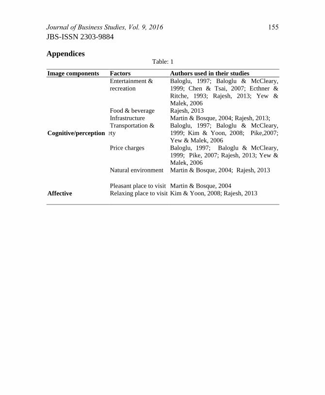
Journal of Business Studies, Vol. 9, 2016 155
JBS-ISSN 2303-9884
Appendices Table: 1
Image components Factors Authors used in their studies
Cognitive/perception
Entertainment &
recreation
Baloglu, 1997; Baloglu & McCleary,
1999; Chen & Tsai, 2007; Ecthner &
Ritche, 1993; Rajesh, 2013; Yew &
Malek, 2006
Food & beverage Rajesh, 2013
Infrastructure Martin & Bosque, 2004; Rajesh, 2013;
Transportation &
Safety
Baloglu, 1997; Baloglu & McCleary,
1999; Kim & Yoon, 2008; Pike,2007;
Yew & Malek, 2006
Price charges Baloglu, 1997; Baloglu & McCleary,
1999; Pike, 2007; Rajesh, 2013; Yew &
Malek, 2006
Natural environment
Martin & Bosque, 2004; Rajesh, 2013
Affective
Pleasant place to visit Martin & Bosque, 2004
Relaxing place to visit Kim & Yoon, 2008; Rajesh, 2013
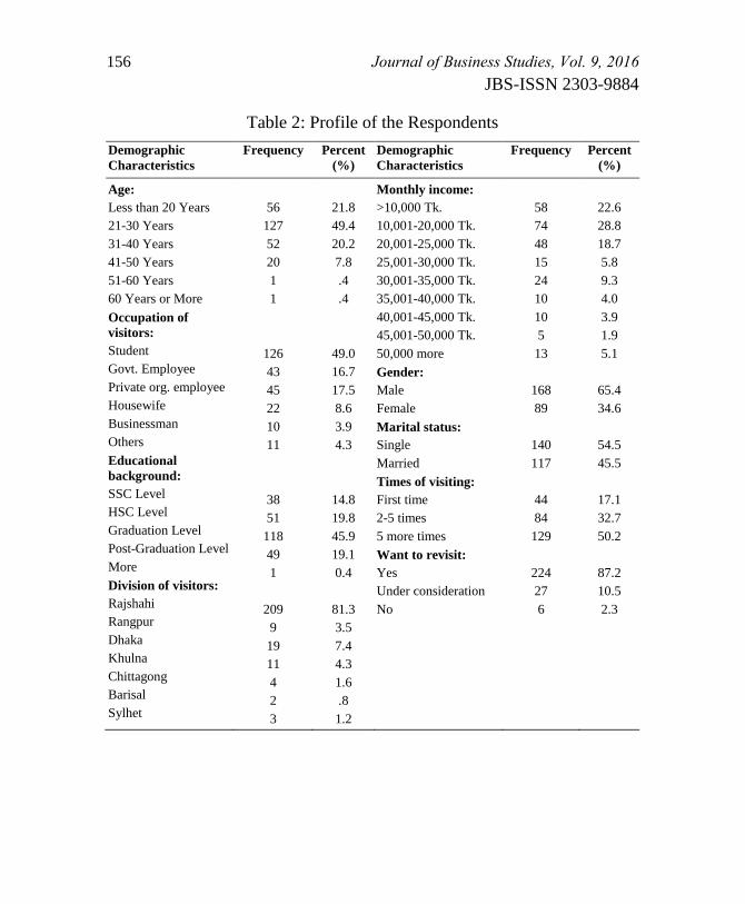
156 Journal of Business Studies, Vol. 9, 2016
JBS-ISSN 2303-9884
Table 2: Profile of the Respondents
Demographic
Characteristics
Frequency Percent
(%)
Demographic
Characteristics
Frequency Percent
(%)
Age:
Less than 20 Years
21-30 Years
31-40 Years
41-50 Years
51-60 Years
60 Years or More
Occupation of
visitors:
Student
Govt. Employee
Private org. employee
Housewife
Businessman
Others
Educational
background:
SSC Level
HSC Level
Graduation Level
Post-Graduation Level
More
Division of visitors:
Rajshahi
Rangpur
Dhaka
Khulna
Chittagong
Barisal
Sylhet
56
127
52
20
1
1
126
43
45
22
10
11
38
51
118
49
1
209
9
19
11
4
2
3
21.8
49.4
20.2
7.8
.4
.4
49.0
16.7
17.5
8.6
3.9
4.3
14.8
19.8
45.9
19.1
0.4
81.3
3.5
7.4
4.3
1.6
.8
1.2
Monthly income:
>10,000 Tk.
10,001-20,000 Tk.
20,001-25,000 Tk.
25,001-30,000 Tk.
30,001-35,000 Tk.
35,001-40,000 Tk.
40,001-45,000 Tk.
45,001-50,000 Tk.
50,000 more
Gender:
Male
Female
Marital status:
Single
Married
Times of visiting:
First time
2-5 times
5 more times
Want to revisit:
Yes
Under consideration
No
58
74
48
15
24
10
10
5
13
168
89
140
117
44
84
129
224
27
6
22.6
28.8
18.7
5.8
9.3
4.0
3.9
1.9
5.1
65.4
34.6
54.5
45.5
17.1
32.7
50.2
87.2
10.5
2.3
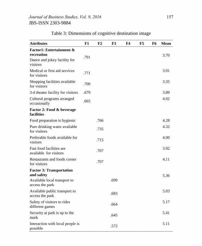
Journal of Business Studies, Vol. 9, 2016 157
JBS-ISSN 2303-9884
Table 3: Dimensions of cognitive destination image
Attributes F1 F2 F3 F4 F5 F6 Mean
Factor1: Entertainment &
recreation
Dance and jokey facility for
visitors
.791
3.70
Medical or first aid services
for visitors .771
3.91
Shopping facilities available
for visitors .700
3.35
3-d theater facility for visitors .679 3.89
Cultural programs arranged
occasionally .665
4.02
Factor 2: Food & beverage
facilities
Food preparation is hygienic .766 4.28
Pure drinking water available
for visitors .735
4.32
Preferable foods available for
visitors .715
4.00
Fast food facilities are
available for visitors .707
3.92
Restaurants and foods corner
for visitors .707
4.11
Factor 3: Transportation
and safety
Available local transport to
access the park
.699
5.36
Available public transport to
access the park .683
5.03
Safety of visitors to rides
different games .664
5.17
Security at park is up to the
mark .645
5.41
Interaction with local people is
possible .572
5.11
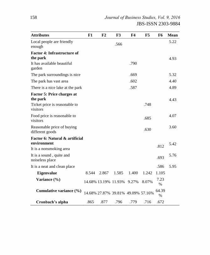
158 Journal of Business Studies, Vol. 9, 2016
JBS-ISSN 2303-9884
Attributes F1 F2 F3 F4 F5 F6 Mean
Local people are friendly
enough .566
5.22
Factor 4: Infrastructure of
the park
It has available beautiful
garden
.790
4.93
The park surroundings is nice .669 5.32
The park has vast area .602 4.40
There is a nice lake at the park .587 4.89
Factor 5: Price charges at
the park
Ticket price is reasonable to
visitors
.748
4.43
Food price is reasonable to
visitors .685
4.07
Reasonable price of buying
different goods .630
3.60
Factor 6: Natural & artificial
environment
It is a nonsmoking area
.812
5.42
It is a sound , quite and
noiseless place .693
5.76
It is a neat and clean place .586 5.95
Eigenvalue 8.544 2.867 1.585 1.400 1.242 1.105
Variance (%) 14.68% 13.19% 11.93% 9.27% 8.07%
7.23
%
Cumulative variance (%) 14.68% 27.87% 39.81% 49.09% 57.16%
64.39
%
Cronbach’s alpha .865 .877 .796 .779 .716 .672
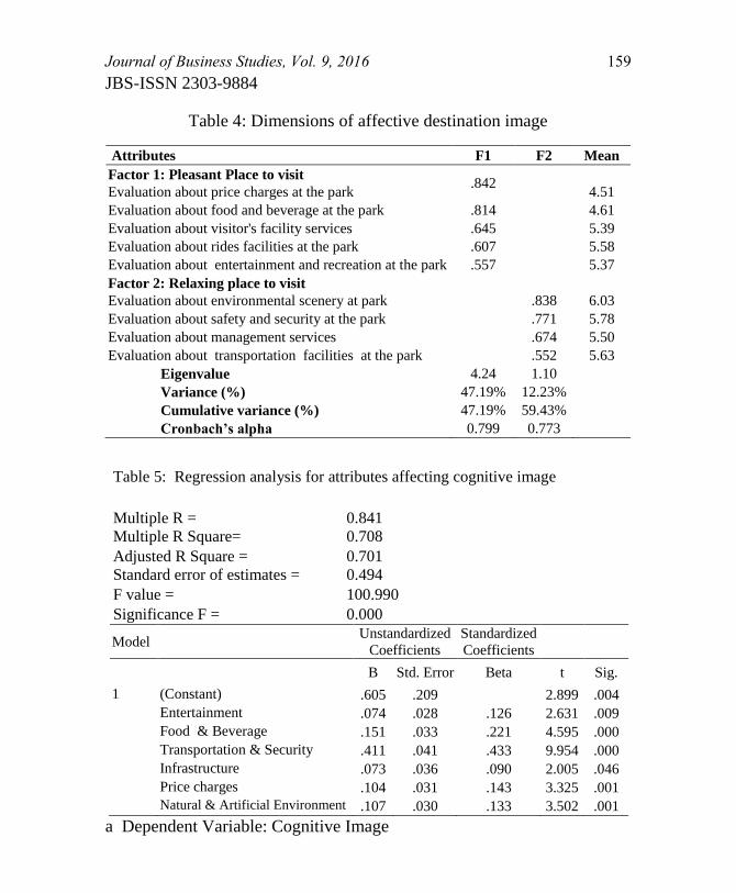
Journal of Business Studies, Vol. 9, 2016 159
JBS-ISSN 2303-9884
Table 4: Dimensions of affective destination image
Attributes F1 F2 Mean
Factor 1: Pleasant Place to visit
Evaluation about price charges at the park .842
4.51
Evaluation about food and beverage at the park .814 4.61
Evaluation about visitor's facility services .645 5.39
Evaluation about rides facilities at the park .607 5.58
Evaluation about entertainment and recreation at the park .557 5.37
Factor 2: Relaxing place to visit
Evaluation about environmental scenery at park
.838
6.03
Evaluation about safety and security at the park .771 5.78
Evaluation about management services .674 5.50
Evaluation about transportation facilities at the park .552 5.63
Eigenvalue 4.24 1.10
Variance (%) 47.19% 12.23%
Cumulative variance (%) 47.19% 59.43%
Cronbach’s alpha 0.799 0.773
Model Unstandardized
Coefficients
Standardized
Coefficients
B Std. Error Beta t Sig.
1 (Constant) .605 .209 2.899 .004
Entertainment .074 .028 .126 2.631 .009
Food & Beverage .151 .033 .221 4.595 .000
Transportation & Security .411 .041 .433 9.954 .000
Infrastructure .073 .036 .090 2.005 .046
Price charges .104 .031 .143 3.325 .001
Natural & Artificial Environment .107 .030 .133 3.502 .001
a Dependent Variable: Cognitive Image
Table 5: Regression analysis for attributes affecting cognitive image
Multiple R = 0.841
Multiple R Square= 0.708
Adjusted R Square = 0.701
Standard error of estimates = 0.494
F value = 100.990
Significance F = 0.000
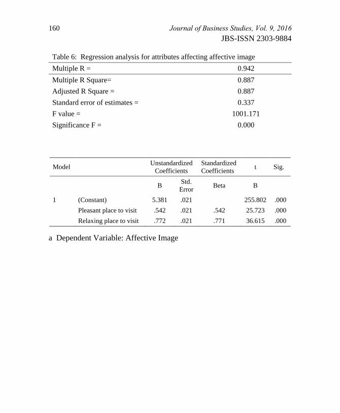
160 Journal of Business Studies, Vol. 9, 2016
JBS-ISSN 2303-9884
Model Unstandardized
Coefficients
Standardized
Coefficients t Sig.
B Std.
Error Beta B
1 (Constant) 5.381 .021 255.802 .000
Pleasant place to visit .542 .021 .542 25.723 .000
Relaxing place to visit .772 .021 .771 36.615 .000
a Dependent Variable: Affective Image
Table 6: Regression analysis for attributes affecting affective image
Multiple R = 0.942
Multiple R Square= 0.887
Adjusted R Square = 0.887
Standard error of estimates = 0.337
F value = 1001.171
Significance F = 0.000

Journal of Business Studies, Vol. 9, 2016 161
JBS-ISSN 2303-9884
Performance Evaluation of Selected NCBs and PCBs in
Bangladesh: An Empirical Study Dr. Mohammad Zahid Hossain1
Md. Fazle Fattah Hossain2
Abstract
There are several ways that the performance of a Bank can be measured. Among
these general business measures and profitability measures are important. In this
study, the performance of selected NCBs and PCBs have been evaluated within a
longer period (1996- 2013). In this study of NCBs and the PCBs, two from the
NCBs and three from the PCBs have been selected. This study has been
conducted on the basis of secondary data which have been collected from some
selected relevant papers. For the analysis of the data regression technique has
been applied. No significant development has been observed from expansion of
branches of Janata Bank Ltd , Rupali Bank Ltd as the NCBs and in terms of
operating profit to total deposit there is no significant achievement of Dutch
Bangla Bank Ltd. as the PCBs. On the other hand in case of Rupali Bank Ltd as
the NCBs no relation has been found in case of authorized capital. Similarly
lower profit has been found against total advance in case of Rupali Bank Ltd as
the NCBs and Jamuna bank Ltd.as the PCBs. From the findings of the analysis it
can be suggested that some parameters i.e. total no. of branches, authorized
capital should be improved for overall development of selected NCBs and the
PCBs.
Keywords: PCBs, NCBs, performance evaluation, general business measures,
regression analysis
(I) Introduction
inancial Institutes and the Non- Financial Institutes are common is all
capitalist form nations. Among these institutions Commercial banks
as a financial institute plays the important role in the country’s overall
development (Karim et al, 2013). Commercial Bank is one of the most
important financial institute. It is called the life blood of any economy.
1 Professor, Department of Finance, University of Rajshahi,
Email: [email protected] 2 Research Fellow, Department of Finance, University of Rajshahi
F
162 Journal of Business Studies, Vol. 9, 2016
JBS-ISSN 2303-9884
These institutions circulate money in the economical functions. These
institutions canalize the money to the deficit unit from the surplus unit.
Thus country’s overall development depends on those financial
institutions. In this way these institutions affect the production of any
economy.
In our globalize world every bank is connected with each other. If one
bank fails to perform well then the effect will create anarchy in the rest
whole banking industry. This also may create a hotchpotch situation in the
country’s economic progress. So it is essential to the concerned
stakeholders in the country to be sincere in supervising and strengthening
the performance of these banks (Karim, 2013).
Generally bank is a collector of deposit and supplier of that deposited
money (Khan,2012).The depositor who want to deposit their hard earned
money can keep their money in return they are given interest or profit. On
the other hand the investors who want to invest in various productive
sectors can borrow fund from those Commercial Banks. So commercial
banks circulates the funds from the surplus unit to the deficit unit (Ahmed
et al; 2011).
At present there are four Nationalized Commercial Banks and almost
thirty nine Private Commercial Banks operating in Bangladesh (Activities
of Bank Insurance and Financial institutions. 2013-2014). These Banks are
playing a greater part in the country’s Development process (Changed
Bangladesh Bank, 2013). In 2007 all the NCBs have made limited
company so that these Banks can take active part in the country’s
development process. On the other hand PCBs are now flourishing. They
are now setting up upazilla level branches as per the directive of the
Bangladesh Bank.
In case of Nationalized Commercial Banks there are several important
aspects, because these organizations have the wide area coverage
including the root level branches. The common people can interact with
them very well. Although they are lacks in terms of customer satisfaction,
they play a good part in the National economy of Bangladesh. They have
to maintain numerous social responsibility, have to disburse agricultural

Journal of Business Studies, Vol. 9, 2016 163
JBS-ISSN 2303-9884
loans to the poor people with a small interests so that they can uplift their
life standard, they have to deposit on a ten taka or hundred taka account
with a healthy interest given, they have to deposit to their school goers and
so on. On the other hand, the Private Commercial Banks are also
flourishing day by day. These organizations are increasing their coverage
according to the directives of the Bangladesh Bank. These banks are
becoming healthier in terms of deposit, advance profit and so on. Their
customer satisfaction and the employee satisfaction have also been
increasing day by day.
However, this research paper has also explored the performance of the
selected NCBs and the PCBs in Bangladesh through the use of regression
equation. With this equation the data have been used depending on
different parameters like deposit, advance, and profit and so on. The
findings have been scrutinized as to whether these selected banks are
performing well and helpful for the management to take corrective
measures. The academician, policy makers have also fore cast the trend of
these parameters so that effective suggestion and the recommendation can
be made more clearly.
Statement of the problem
Banking industry in Bangladesh is now facing numerous challenges. In
case of Nationalized Commercial Banks there are so many problems that
need to be addressed like problems incase of deposit collection, incase of
disbursing loan, in case of political influence and so on. On the other hand,
the private commercial banks are facing some problem regarding their
expansion of branches, their corruption into their internal management in
disbursing the loan, regarding their CSR and some other activities. So it is
time to un- earth the performance of those NCBs and the PCBs to see
whether it creates any negative impact in terms of profitability and in
general business measures.
General objective
To evaluate the performance of some selected NCBs and PCBs in terms of
General Business Measures and Profitability.
164 Journal of Business Studies, Vol. 9, 2016
JBS-ISSN 2303-9884
Specific objectives
a) To depict the general picture of some selected NCBs and the PCBs
in Bangladesh.
b) To depict the growth rate of some selected NCBs and the PCBs in
terms of general business measures and profitability measures.
c) To evaluate the performance of some selected NCBs and the PCBs
in terms of General Business Measures and Profitability Measures.
(II) Methodology
A systematic research may be conducted through applying several study
methods like social survey, case study, observation and so on. But in this
study content analysis has been used as the progressive report and other
publication of Banks contain authentic data as because these reports are
based on the audited document. That is why only content analysis method
has been applied for getting the practical rigorous result of the topic.
Sources of data and data collection
For evaluating and measuring performance of the selected banks as per the
research objectives, secondary data from the different sources like Govt.
report, official record, various books, journal, and annual report of
respective banks have been consulted.
Sample and selection of sample
In any scientific study certain percentage of sample is usually collected for
conducting the study. But in this study the required percentage is not
maintained. However the finding of the study is representative and
trustworthy as the nature of the data is almost homogenous in nature. So
from the NCBs and the PCBs, two Banks from the NCBs and three Banks
from the PCBs have been taken. The NCBs are Janata Bank Ltd, Rupali
Bank Ltd. The PCBs are Islami Bank Ltd., Dutch Bangla Bank Ltd. and
Jamuna Bank Ltd. These Banks are generally called the first generation,
second generation and third generation commercial banks.
Journal of Business Studies, Vol. 9, 2016 165
JBS-ISSN 2303-9884
Reference period
The secondary data from the above mentioned banks have been taken for
the period of 1996 to 2013.
Data analysis
Firstly data have been collected and tabulated. The growth rates of
different parameter have been calculated using excel program. So many
analysis techniques like ratio analysis, EVA model, AHP model, CAMEL
rating etc. can be used however considering suitability and easy applicable
in this field the performance has been evaluated using the regression
analysis on the basis of General Business Measures and the profitability
Measure. In this regard Eviews-8 has been uses. The above measure has
been used because it can depict the actual scenario of any Banks.
The model
y= ß1 + ß2 x + e
where y the dependent variable or the regressand indicates the trend in
years of the different parameters ß1 the intercept term ß2 is the slope
coefficient and x is the independent variable or the explanatory variable
indicates the performance indicator or parameter of the Banks like deposit,
advance, total assets etc.
(III) Review of Literature
An article titled “Performance Evaluation of Selected Private Commercial
Banks in Bangladesh” is an important article by Ahmed et. al. (2009).The
objective of the study is to synthesize the growth and development of
some private commercial banks. Secondary data from various sources
were used. The study used numerous statistical tools like growth
percentage, trend equation, square of correlation coefficient, correlation
matrix etc. From the analysis of the trend equation it was found that the
growth trend of branches, deposit, and the net income is significant.
Popa et. al. (2009) observed in their article titled “An Advance Methods
for the Performance Evaluation of Banks”. The Advanced Method for the
Performance Evaluation of Banks performance is called the EVA. The
authors tried to examine the Banks performance .In USA it were widely
166 Journal of Business Studies, Vol. 9, 2016
JBS-ISSN 2303-9884
used to measure the Banking performance. The aim of the study is to
implement this technique in measuring the performance of the Banking
industry side by side in comparison of other technique. This method
usually includes the return on assets, return on equity, banking income etc.
The main advantages of the methods consist of in the management system,
in case of motivation, incase of measurement.
An article titled “Evaluating the performance of Commercial Banks in
India” by Malhotra et. al. (2011). The authors tried to examine the
different performance indicators like profitability, cost of intermediation,
efficiency and so on. Secondary data were used in the study. The study
used the descriptive statistics to measure the performance of Banks in the
different dimensions. The result showed that the enhancement of the net
interest margin, rising of the cost of intermediation and so on created
competition among the banking industry.
An article contains “Performance Evaluation of Scheduled Commercial
Banks in India” is an important article by Gurusamy and his co authors
(2013). The aim of the study was to measure the growth of the entire
schedule Commercial Banks and to make the comparison among the
different commercial banks. The study used descriptive statistics like
standard deviation, coefficient of variation; mean and so on the result
showed that the FBs were the highest mean among three groups. But in
case of NPA both of FBs and PSBs were experienced uniform services in
terms of the deposit, advance, income, interest income and so on. And also
FBs secured first place employee, profit per employee, and percentage of
wages to total expenditure.
Malhotra et. al. investigated the performance appraisal of banking sector
in their article titled “Performance Appraisal of Indian Public Sectors
Banks”. In this study the authors tried to evaluate the performance of the
public sectors Banks. The study used CAMEL rating technique to evaluate
the performance level of the Banks .The result found that Bank of Baroda
was excellent. On the other hand Bank of Andhra was average .Lastly the
Bank of Maharashtra and United Bank were positioned at the bottom.
Journal of Business Studies, Vol. 9, 2016 167
JBS-ISSN 2303-9884
Kaur (2012) in his article titled “An Empirical Study on the Performance
Evaluation of Public Sector Banks in India” pointed out the performance
evaluation of Indian public sector Banks. In this study the authors tried to
emphasize the profitability measures of Public sectors Banks in India also
analyzed the non performing assets of the commercial Banks. The study
used coefficient of correlation, chi square test, median, etc .The result
revealed that there were high positive correlation between the profitability
and the interest earned, and there exists no significance difference between
the growth rates, total income, total expenditure, and the net profit of
PSCBs and SCB in India.
Sangmi studied the Financial Performance of Commercial Banks in India
in his article titled “Analyzing Financial Performance of Commercial
Banks in India: Application of CAMEL Model”. In this article the authors
tried to gain an insight into the performance of the two major banks using
the CAMEL rating technique. The study focused that the two banks were
remain in good position in terms of capital adequacy, asset quality, and
Management capability and so on. The study revealed that both the two
banks had been doing well in every aspect like capital adequacy, asset
quality, and management capability and so on.
A study conducted by Richard et al (2013) titled “The Determinant of
Financial Performance of Quoted Banks in Nigeria”. The study tried to
analyze the determinant that affects the financial performance of Banks.
The article used the secondary data from the various sources from the
three Banks. The statistical tools regression analysis had been used to
determine the trend of the different parameters. The study revealed that the
asset qualities growth trend was significant.
An article titled “AHP based Model for Bank Performance Evaluation and
Rating” is an important article by Hunjak et.al; (2001).The article used
Analytical Hierarchy Process. This process explains the internal and the
external factors of Banks. The Analytical Hierarchy process examines the
quantity and the quality based criteria .It is a multi criteria evaluation
models that enables the measurement of the subjective assessment of the
study.

168 Journal of Business Studies, Vol. 9, 2016
JBS-ISSN 2303-9884
“An Evaluation of Financial Performance of Private Commercial Banks in
Bangladesh: Ratio Analysis” in an important study by Karim et. al; The
aim of the study was to find out the financial performance of the private
Commercial Banks using the ratio analysis. Economic Value Added had
been used to measure the liquidity ratio, return on assets, return on equity
and so on. The result showed that the Bank size, credit risk, operational
efficiency and the asset management were significant.
Raihan et. al. found the performance of State Owned Commercial Banks
in their article titled “Performance Evaluation and Competitive Analysis
of State Owned Commercial Banks in Bangladesh” The aim of the study
was to find the performance of the state owned commercial Banks. The
study used the secondary data for the analysis. The regression analysis was
used to un-earth the actual scenario of performance of the State Owned
Commercial banks in Bangladesh. The study found that these Banks were
not able to achieve the steady growth in terms of net profit, earning per
share, return on equity, and return on assets and so on. On the other hand it
achieved the stable growth in terms of general business measures.
Choong et. al. measured the performance of Islamic Commercial Banks in
Malaysia in their article titled “Performance of Islamic Commercial Banks
in Malaysia: An empirical study”. The study tried to gain an insight into
the most important performance indicators that is responsible for the
overall performance of the banks. The study used the regression model to
find the important indicator of the performance. The result revealed that
the credit risk was the important determinant of performance of Islamic
Commercial Banks in Malaysia.
From the above literature review from different sources it is evident that
there exist so many articles relating to the performance evaluation.
Different study uses different methods to un-earth the true picture of the
commercial Banks. The current study tries to determine the actual picture
of the Commercial Banks of Bangladesh using the longer study period and
also by exact statistical tools.

Journal of Business Studies, Vol. 9, 2016 169
JBS-ISSN 2303-9884
(IV) Concept and Definitions
NCBs
NCBs: It is generally called the Nationalized Commercial Banks. There
are four NCBs in Bangladesh (Activities of Banks, Insurance and
Financial Institutions 2013-2014). These includes Sonali Bank Limited,
Janata Bank Ltd., Agrani Bank Ltd and Rupali Bank ltd,Basic Bank Ltd
and Bangladesh Development Bank Ltd. After the liberation war first four
Banks had been Nationalized by the then Govt. of Bangladesh. Prior to the
Nationalization, those Banks had been operating under different name and
are now operating under the Bank Company Act and direct control of the
government of Bangladesh.
PCBs
It is generally called the Private Commercial Banks. At present there are
almost thirty nine PCBs are operating in our country (Activities of Banks,
Insurance and Financial Institutions 2013-2014).These include the first
generation, second generation and the third generation Private
Commercial Banks. These Banks are also operating by the Bank Company
Act.
Janata Bank Limited
Janata Bank is one of the leading Nationalized Commercial Banks in
Bangladesh. Janata Bank was formed by merging United Bank Ltd and
Union Bank Ltd in 1972 according to President Order-26. In 2007 Janata
Bank started as a limited company. The Authorized capital amounted to
Tk 20000 million, Paid up capital amounted to Tk. 19140 million at the
end of December 2013.Janata Bank limited has 893 branches and the
employees is almost 15370. Bank participate in the socio economic
development of Bangladesh side by side the Bank provides loans in
various productive purposes and collects deposit from the depositors(
Activities of Banks , Insurance Companies and Financial institutions
2013-2014)
Rupali Bank Limited
The fourth Nationalized Commercial Banks in Bangladesh is the Rupali
Bank Limited. The Bank was formed by merging the Muslim Commercial
170 Journal of Business Studies, Vol. 9, 2016
JBS-ISSN 2303-9884
Bank Limited, Standard Bank Limited and Australasia Bank Limited in
1972 according to the President Order-26. The Authorized capital
amounted to Tk. 7000 million, Paid up capital amounted to tk.1815
million at the end of December 2013.Rupali Bank limited has 532
branches and the employees is almost 5669. (Activities of Banks,
Insurance Companies and Financial institutions 2013-2014)
Islamic Bank Limited
The largest first generation Private Commercial Banks in Bangladesh is
the Islamic Bank Limited. The Bank was formed in 1983 as a public
limited company and started interest free Banking at the same year. The
major partnership of the Bank includes Islami Development Bank, some
of foreign Financial Institute, and Foreign entrepreneur. The Authorized
capital amounted to Tk 20000 million, Paid up capital amounted to tk.
14636 million at the end of December 2013.The Bank has almost 286
branches and the employees is almost 12000. Banks participate in the
socio economic development of Bangladesh and side by side the Bank
provides loans to various productive purposes and collects deposit from
the depositors. The Bank is the pioneer to launch Islami Banking activity
according to the Islami Sariah and engaged in different Musharaka
project. Also Bank has different Mudaraba savings scheme by which it
collects deposit from the investors (Activities of Banks, Insurance
Companies and Financial institutions 2013-2014)
Dutch Bangla Bank Limited
The largest second generation Private Commercial Banks in Bangladesh is
the Dutch Bangla Bank Limited. The Bank was formed in 1996 as a public
limited company and started its Banking business. The major partner of
the Bank includes the Nederland Development Finance Company and
Bangladeshi entrepreneurs. The Authorized capital amounted to Tk 4000
million, Paid up capital amounted to Tk 2000 million at the end of
December 2013.The Bank has almost 136 branches and the employees is
almost 4666. Bank participates in the socio economic development of
Bangladesh and side by side the Bank provides loans to various productive
purposes and collects deposit from the depositors. The Bank is the pioneer
to launching the mobile banking in Bangladesh; also initialize the
Journal of Business Studies, Vol. 9, 2016 171
JBS-ISSN 2303-9884
Electronic Student Booth (Activities of Banks, Insurance Companies and
Financial institutions 2013-2014)
Jamuna Bank Limited
The third generation private Commercial Banks in Bangladesh is the
Jamuna Bank Limited. The Bank started its operation in 2001. The
Authorized capital amounted to Tk10000 million, Paid up capital
amounted to tk. 4488 million at the end of December 2013.Jamuna Bank
limited has 91 branches and the employees is almost 2100. Bank
participates in the socio economic development of Bangladesh and side by
side the Bank provides loans to various productive purposes and collects
deposit from the depositors. The Bank initialize the Islami Banking,
disbursing relief to the poor, set up swing training center, establish Jamuna
Bank Model village and so on(Activities of Banks , Insurance Companies
and Financial institutions 2013-2014)
Hypothesis of the Study
Ho = There is no difference between two types of banks performance.
H1 = There may have some differences between two types of banks in
terms of general business measures and profitability measures.
H2 = Let it be justified, measured and evaluated to what extent the
difference is existing.
(V) Analysis and Findings
General Business Measures
Growth of total investment of the selected NCBs and PCBs
From the table-1 it has been found that there is stable growth rate in case
of Janata Bank except in 2003 and 2006.In case of Rupali Bank growth
rate is positive except in 2004,05 and06.Incase of all the years growth rate
is positive except in 2005 and 2008.In case of DBBL the growth rate is
positive except in 2003,2004 and 2011.Lastly in case of Jamuna Bank
growth rate is positive except in 2002,2003 and 2013.

172 Journal of Business Studies, Vol. 9, 2016
JBS-ISSN 2303-9884
r-square value total investment of selected NCBs and PCBs
From the table- 2 it has been found that highest r-square value is for
Dutch Bangla Bank Ltd (0.885) as the PCBs and the lowest value is for
Islami Bank Bangladesh Ltd (0.572) as also PCBs .So the performance of
PCBs has been better than NCBs in case of total investment activities.
Growth of total deposit of the selected NCBs and PCBs
From the table-3 and from the growth trend it has been found that there is
stable growth rate in case of Janata Bank except in 2003.In case of Rupali
Bank growth rate is positive except in 1997 and 2008.In case of Islami
bank Ltd all the years growth rate if positive. In case of DBBL all the
year’s growth rate is positive. Lastly in case of Jamuna Banks Ltd. deposit
growth rate is positive.
r-square value of total deposit of selected NCBs and PCBs
From the table- 4 it has been found that the highest value of r-square value
in case of Islami Bank Bangladesh Ltd (0.904) as the PCBs and lowest
value has been found for Rupali Bank Ltd. (0.777)as the NCBs. Hence it is
clear that performance of PCBs is better than performance of NCBs.
Growth of total branches of the selected NCBs and PCBs
From the table-5 it has been found that there is stable growth rate in case
of Janata Bank except in 2002 and 2003.In case of Rupali Bank growth
rate in 1998.1999., 2002, and 2003 is negative. Incase of Islami Bank Ltd
all the years’ growth rate is positive .In case of DBBL in 2003 growth rate
is zero.
r-square value of total branches of selected NCBs and PCBs
From the table- 6 it has been found that the higher r-square value in case
of Jamuna Bank Ltd (0.968) as the PCBs and the lowest value has been for
Janata Bank Ltd (0.191) as the NCBs. This shows that PCBs has been able
to maintain the required growth in case of expansion of branches on the
other hand NCBs has not been able to maintain the required growth.
Journal of Business Studies, Vol. 9, 2016 173
JBS-ISSN 2303-9884
Growth of total operating profit of the selected NCBs and PCBs
From the table-7 it has been found that there is stable growth rate in case
of Janata Bank is positive except in 1998, 2002, 2012, and 2013(according
to June 2013).In case of Rupali Bank growth rate is not satisfactory. In
case of Islami Bank the growth rate if positive except in 1997, 1998,
2000,2003,2004,2006 and 2013 and 2013.In case of DBBL the growth rate
is satisfactory except 1997,1998,2003,2009, and 2013. Lastly in case of
DBBL in 2013 is not satisfactory and lastly Jamuna Bank growth rate is
satisfactory.
r-square value of total operating profit of selected NCBs and PCBs
The higher r-square value from the table- 8 has been found in case of
Jamuna Bank Ltd(0.884) as the PCBs and the lower value has been found
for Rupali Bank Ltd. (0.656) as the NCBs .Hence we can conclude that
PCBs has been in healthier position in terms of the operating profit than
NCBs.
Growth of manpower of the selected NCBs and PCBs
From the table-9 it has been found that the growth rate of Manpower is not
satisfactory in case of Janata Bank. In case of Rupali Bank growth rate is
also not satisfactory. Incase of Islami Bank all the years growth rate if
positive. In case of DBBL the growth rate is negative in 2004 and 2013
and the Jamuna Banks Manpower growth rate is satisfactory.
r-square value of manpower of selected NCBs and PCBs
From the table10 it has been found that the highest r-square value is for
Jamuna Bank Ltd.(0.943) as the PCBs and the lowest value has been
found for Rupali bank Lid.(0.424) as the NCBs. This means that PCBs
have been well ahead in case of recruiting of manpower than the NCBs.
Growth of total advance of the selected NCBs and PCBs
From the table-11 it has been found that there the growth rate in 1998 and
2007 is negative in case of Janata Bank Ltd. In case of Rupali Bank
growth rate is positive except in 2005. Incase of all the three PCBs the
growth rate is positive.

174 Journal of Business Studies, Vol. 9, 2016
JBS-ISSN 2303-9884
r-square value of total advance of selected NCBs and PCBs
From the table- 12 higher r-square value has been found for Jamuna
Bank Ltd. (0.978) as the PCBs and lower value has been found for Rupali
bank Ltd.(0.823) as the NCBs.Hence we can conclude that PCBs
performance is better than NCBs performance in terms of the advance.
Growth of inland remittance of the selected NCBs and PCBs
From the table-13 it has been found that the growth rate is negative in
1999,2003,2010,2011 and in case of JBL. In case of Rupali Bank growth
rate is negative in 1997, 1999, 2001, 2010, 2013. Incase of Islami Bank all
the years growth rate is positive except in 2000and 2013. In case of DBBL
the growth rate is negative in 1999,2000,2003,2005 and .In case of
Jamuna Bank Ltd. (JBL) the growth rate is negative in 2009, 2010 and.
r-square value of inland remittance of selected NCBs and PCBs
From the table- 14 it has been found that the maximum r-square value for
Janata Bank Ltd.(0.863) as the NCBs and the lowest for Dutch Bangla
Bank Ltd.(0.734) as the PCBs. So NCBs performance is better than PCBs
performance in case of inland remittance.
Growth of total assets of the selected NCBs and PCBs
From the table-15 it has been found that in case of JBL the growth rate in
2003 is negative and in case of RBL the growth rate in 2000 is negative. In
case of all the PCBs growth rate of total Assets is satisfactory.
r-square value of total assets of selected NCBs and PCBs
From the table- 16 the r-square value of Jamuna Bank Ltd has been found
higher (0.875) as the PCBs and lower value has been found for Rupali
Bank Ltd.(0.739) as the NCBs. So PCBs performance has been better in
comparison to the NCBs performance.
Growth of paid up capital of the selected NCBs and PCBs
From the table-17 it has been found that there exists no steady growth in
case of Paid up Capital except the Islami Banks and Jamuna Banks.
Journal of Business Studies, Vol. 9, 2016 175
JBS-ISSN 2303-9884
r-square value of paid up capital of selected NCBs and PCBs
From the table- 18 the r-square value has been maximum for jamuna Bank
ltd.(0.835) as the PCBs and the minimum value has been for Rupali Bank
Ltd.( 0.357) as the NCBs . It shows PCBs performance has been better
regarding the paid up capital.
Growth of total authorized capital of the selected NCBs and PCBs
From the table-19 it has been found that there exists no stable growth rate
in all the five NCBs and the PCBs
r-square value of total authorized capital of selected NCBs and PCBs
The r-square value from the table- 20 Islami Bank Bangladesh Ltd as the
PCBs has the highest value (0.808) and no value has been found for
Rupali Bank Ltd as the NCBs. So PCBs performed well in comparison to
the NCBs in case of authorized capital.
Growth of total import of the selected NCBs and PCBs
From the table-21 it has been found that the growth rate in 1997, 1999,
2005,2007,2009,2012 and 2013 shows the negative trend. In case of RBL
the growth rate 1999, 2002, 2005, 2006, 2012 and shows the negative
trend. In case of Islami Bank the growth rate in 1997, 2000, 2009, 2012,
and also shows the negative trend. In case of DBBL the growth rate in
2011 and 2013 is negative .Finally in case of Jamuna bank ltd the growth
rate in 2011 and 2013 is negative.
r-square value of total import of selected NCBs and PCBs
From the table- 22 the r-square value for Jamuna Bank has been found
maximum (0.910) as the PCBs and minimum value (0.629) has been
found for Rupali bank Ltd as the NCBs. So PCBs performed well in case
of import activities.
Growth of total export of the selected NCBs and PCBs
From the table-23 it has been found that the growth rate in case of JBL in
1998 is negative. In case of RBL the growth rate in 2001, 2002, 2004,
2005, 2007, 2009, and 2013 is negative .In case of IBBL in 2002, 2013 the
176 Journal of Business Studies, Vol. 9, 2016
JBS-ISSN 2303-9884
growth rate is negative .In case of DBBL and the Jamuna Bank Ltd the
growth rate is negative in 2012
r-square value of total export of selected NCBs and PCBs
The r-square value from the table- 24 it has been found maximum value
for Janata bank Ltd.(0.891) as the NCBs and minimum value has been for
Rupali Bank Ltd(0.507). This shows the better position of NCBs in case of
export business.
Growth of gross income of the selected NCBs and PCBs
From the table-25 it has been found that in case of JBL the growth rate is
negative in 1998, 2004.In case of RBL the growth rate is negative in 2004,
2008.
r-square value of gross income of selected NCBs and PCBs
the r-square value from the table- 26 it has been found maximum for
Jamuna Bank Ltd.(0.885) as the PCBs and minimum value has been found
for Rupali Bank Ltd.(0.736) as the NCBs. Hence PCBs generate higher
gross income in comparison to the NCBs.
Growth of operating expenditure of the selected NCBs and PCBs
From the table-27 it has been found that the growth rate is shows the
negative trend in the year 2001, 2003, 2004 in case if JBL. In case of RBL
the growth rate in negative in 2002, 2004, 2008.
r-square value of operating expenditure of selected NCBs and PCBs
From the table- 28 the r-square value has been found for Jamuna Bank
Ltd.(0.885) as the PCBs and the lowest value has been for Rupali Bank
ltd(0.624) as the NCBs.So PCBs expenditure has been higher than the
NCBs expenditure.
Profitability Measures
Growth of total operating profit to total advance of the selected NCBs
and PCBs
From the table-29 it has been found that there exists no stable growth in all
the five NCBs and the PCBs.
Journal of Business Studies, Vol. 9, 2016 177
JBS-ISSN 2303-9884
r-square value of total operating profit to total advance of selected
NCBs and PCBs
From the table- 30 r-square has been found in case of Islami Bank
Ltd.(0.871) as the PCBs and lower value has been found for Jamuna Bank
Ltd.(0.216).So it has been observed that PCBs performance is better than
NCBs performance.
Growth of total operating profit to total deposit of the selected NCBs
and PCBs
From the table-31 it has been found that there exists no stable growth in all
the five NCBs and the PCBs.
r-square value of total operating profit to total deposit of selected
NCBs and PCBs
The r-square value from the table- 32 it has been observed that higher
value for Janata Bank Ltd.(0.789) and lower value for Dutch Bangla Bank
Ltd.(0.270). Hence it has been concluded that NCBs performance is better
than PCBs performance.
(VI) Conclusion
The performance evaluation of Banks means how and what level the
Banks performance exists. If the Banks performs well, the Bank has to do
well in every parameter. The parameter means deposit, advance, profit,
investment, assets, import, export, and so on. All these parameter are the
raw material to evaluate the level of performance. In this research that has
considered the general business measures we see that growth rate of total
investment, total no. of Branches, and total no. of Manpower, Inland
remittance, total import, total export, operating expenditure, total advance
and operating profit of the NCBs are not satisfactory. In the case of PCBs
Inland remittance and Paid up Capital for Dutch Bangla Bank Ltd. ,
Authorized capital for all the selected PCBs, Total import for Islami Bank
Bangladesh Bank Ltd., total operating profit to Total advance for all the
selected PCBs are not satisfactory. Again it is clear that there exists no
significant trend in case of Janata Bank Ltd and Rupali Bank Ltd. as the
NCBs in terms of branches. Higher and significant r-square value has been
found in case of total investment, Deposit, Expansion of Branches,

178 Journal of Business Studies, Vol. 9, 2016
JBS-ISSN 2303-9884
Operating Profit, Manpower, Advance, total Assets, Paid up Capital,
Authorized Capital, Import, Gross income of PCBs. On the other hand
Higher and significant R-square value has been found in case of Inland
Remittance, Export and lowest value of operating expenditure of NCBs.
Hence we can conclude that for considering most of the parameter of
general business measures PCBs performance has been better than the
NCBs performance.
Recommendations
From the analysis the Banks should take the following steps to enhance
their healthy business or the profitability:
a) The PCBs should collect deposit from the various sources in the
name of different scheme.
b) The NCBs should set up more branches.
c) The RBL as NCBs should recruit more employees for enhancing
profitability.
d) The NCBs should improve the condition of the paid up capital and
the authorized capital.
e) The DBBL and the Jamuna Bank Ltd as PCBs should improve the
condition of advance.
Limitation of the study
a) The study depends only on secondary data from various sources
and the whole study is based on the accuracy of those data.
b) Limited number of selected Banks for unveiling the actual scenario
of Banking Industry in Bangladesh
Journal of Business Studies, Vol. 9, 2016 179
JBS-ISSN 2303-9884
References
Abedin, M. Zainul. “Commercial banking in Bangladesh: A Study of
Disparities of Regional and Sectoral Growth Trends (1846-1986).”
Unpublished Ph.D. Dissertation, Rajshahi: IBS, Rajshahi University,
1988.
Ahmed, Mahmood. “Growth of Industrial Entrepreneurship in Bangladesh”.
Unpublished Ph.D. thesis, Institute of Bangladesh Studies, Rajshahi
University, Rajshahi, 1993.
Akkas, S.M. Ali. “Relative Efficiency of Conventional and Islamic Banking
Systems in Financing Investment”. Unpublished Ph.D. thesis, Dhaka
University, Dhaka, 1996.
Alam, Ahmed Farkrul. Company Law. Dhaka: Royal Library, 2004.
Alam, M. Badiul. “Organizational Effectiveness of Public Enterprise in a
Developing Economy: A Study of Sugar Industry in Bangladesh”
Unpublished Ph.D. Dissertation, Rajshahi: IBS, Rajshahi University,
1992.
Ali, A. Yousuf. Trans. The Holy Quran : Text, Translation and
Commentary. Maryland, USA : Amana Corporation, 1983.
Ali, A.F.M. Ashraf. “Management of Agricultural Credit: A Study of the
Bangladesh Krishi Bank in Rajshahi District”. Ph.D. thesis,
Institute of Bangladesh Studies, Rajshahi University, Rajshahi,
1983.
Allen, William R. and Bragaw, Lewis. Social Forces and the Manager.
New York: Wiley, 1982.
Andrews, K.R. The Concept of Corporate Strategy. Homewood, IL:
Richard D. Irwin, 1980.
Andrews, Kenneth. The Concept of Corporate Strategy. Homewood,
Illinois: Dow-Jones Irwin, 1971.
180 Journal of Business Studies, Vol. 9, 2016
JBS-ISSN 2303-9884
Anjum, Md. Nasim, “Entrepreneurship” Development in The Northern
Districts of Bangladesh.” Unpublished Ph.D. Dissertation, Rajshahi:
Department of Management, Rajshahi University, 1995.
Ashis Bandari and Amrit Man Nakarmi(2014) “Performance Evaluation of
Commercial Banks in Nepal Using AHP”.International Journal of the
Analytic Hierarchy Process.june 29-july 2,p 1-5.
Avneet Kaur (2012) “Performance Evaluation of Consolidated Banks in
Nigeria by Using Non-Financial Measures”.
Awwal, AZM Iftikhar. The Industrial Development of Bengal 1900-1939.
Dhaka University Press, 1975.
Baran, Michael S. Alternatives to Regulation. Lexington, Mass: Lexington
Books Heath, 1982.
Becker, Gary S. Human Capital. New York: Columbia University Press,
1964.
Berenson, Conrad and Eilbirt, Henry. The Social Dynamics of Marketing.
New York: Random House, 1973.
Berle, Adolph A. and Means, Gardiner C. The Modern Corporation and
Private Property. New York: Macmillan, 1933.
Bhuyan, Ayubur Rahman and Rashid, Mohammad Ali. Trade Regimes
and Industrial Growth: A Case Study of Bangladesh. Dhaka:
Bureau of Economic Research, 1993.
Boulton, W.R. Business Policy: The Art of Strategic Management. New
York: Macmillan, 1984.
Bowen, Howard R. Social Responsibilities of Businessman. New York:
Harper and Prothers, 1953.
Bursk, Edward C. Business and Religion. New York: Harper & Row
Publishers, 1959.
Journal of Business Studies, Vol. 9, 2016 181
JBS-ISSN 2303-9884
Choudhury, Toufic Ahmed. “An Evaluation of the Performance of
Commercial Banks of Bangladesh.” Ph.D. Dissertation, Department
of Economics, Himachal Pradesh University, 1990.
Gunu Umar and Olabisi Jimoh Olatunde (2011).Interdisciplinary Journal
of Research in Business.vol 1,Issue 9, sep-oct,p72-83
Habibullah, M. and Ahmed, Mahbub. “Study on Social Profitability and
Nationalized Commercial Banks.” Dhaka: National Commission on
Money, Banking and Credit, 1985 (Mimeographed).
Rashed Al Karim and Tamima Alam (2013). An Evaluation of Financial
Performance of Private Commercial Banks in Bangladesh: Ratio
Analysis. Journal of Business Studies Quarterly. Volume 5 p 65-
77.
Shah Johir Rayhan, S.M. Sohel Ahmed and Ripon Kumar Mondal (2011).
Performance Evaluation and Competitive Analysis of State Owned
Commercial Banks in Bangladesh. Research Journal of Finance
and Accounting. Vol 2, No 3, p 99-113.
Tihomir Hunjak and Drago Jakovcevic (2001) “Ahp Based Model for
Bank Performance Evaluation and Rating”. ISAHP 2001, Berne,
Switzerland, August 2-4,2001 p 149-157.
Yap Voon Choong,Chan Kok Thim and Bermet Talasbek Kyzy (2012)
“Performance of Islamic Commercial Banks in Malysia: An
empirical Study”.Journal of Islamic Economics, Banking and
Finance, vol 8 no.2 April-June 2012, p 68-80.
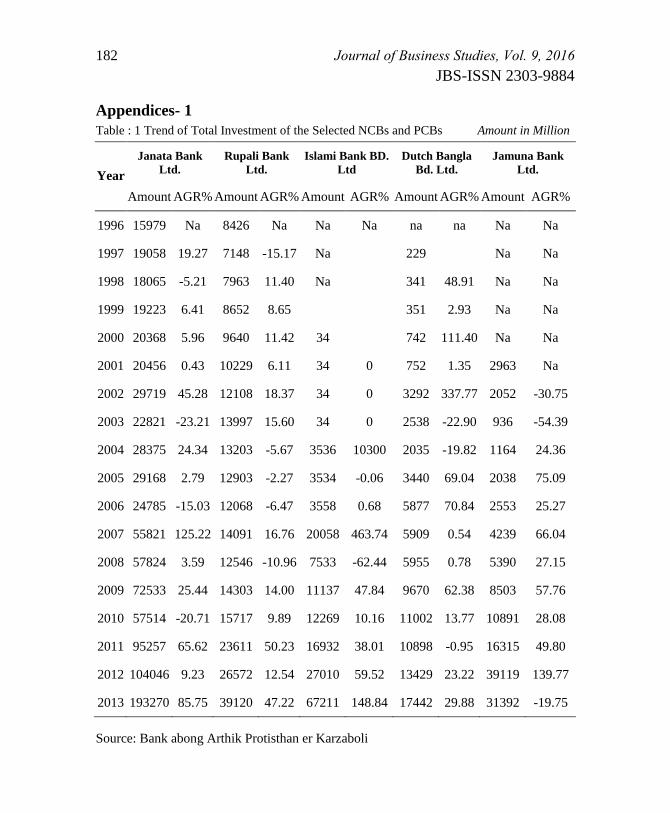
182 Journal of Business Studies, Vol. 9, 2016
JBS-ISSN 2303-9884
Appendices- 1
Table : 1 Trend of Total Investment of the Selected NCBs and PCBs Amount in Million
Year
Janata Bank
Ltd.
Rupali Bank
Ltd.
Islami Bank BD.
Ltd
Dutch Bangla
Bd. Ltd.
Jamuna Bank
Ltd.
Amount AGR% Amount AGR% Amount AGR% Amount AGR% Amount AGR%
1996 15979 Na 8426 Na Na Na na na Na Na
1997 19058 19.27 7148 -15.17 Na 229 Na Na
1998 18065 -5.21 7963 11.40 Na 341 48.91 Na Na
1999 19223 6.41 8652 8.65 351 2.93 Na Na
2000 20368 5.96 9640 11.42 34 742 111.40 Na Na
2001 20456 0.43 10229 6.11 34 0 752 1.35 2963 Na
2002 29719 45.28 12108 18.37 34 0 3292 337.77 2052 -30.75
2003 22821 -23.21 13997 15.60 34 0 2538 -22.90 936 -54.39
2004 28375 24.34 13203 -5.67 3536 10300 2035 -19.82 1164 24.36
2005 29168 2.79 12903 -2.27 3534 -0.06 3440 69.04 2038 75.09
2006 24785 -15.03 12068 -6.47 3558 0.68 5877 70.84 2553 25.27
2007 55821 125.22 14091 16.76 20058 463.74 5909 0.54 4239 66.04
2008 57824 3.59 12546 -10.96 7533 -62.44 5955 0.78 5390 27.15
2009 72533 25.44 14303 14.00 11137 47.84 9670 62.38 8503 57.76
2010 57514 -20.71 15717 9.89 12269 10.16 11002 13.77 10891 28.08
2011 95257 65.62 23611 50.23 16932 38.01 10898 -0.95 16315 49.80
2012 104046 9.23 26572 12.54 27010 59.52 13429 23.22 39119 139.77
2013 193270 85.75 39120 47.22 67211 148.84 17442 29.88 31392 -19.75
Source: Bank abong Arthik Protisthan er Karzaboli
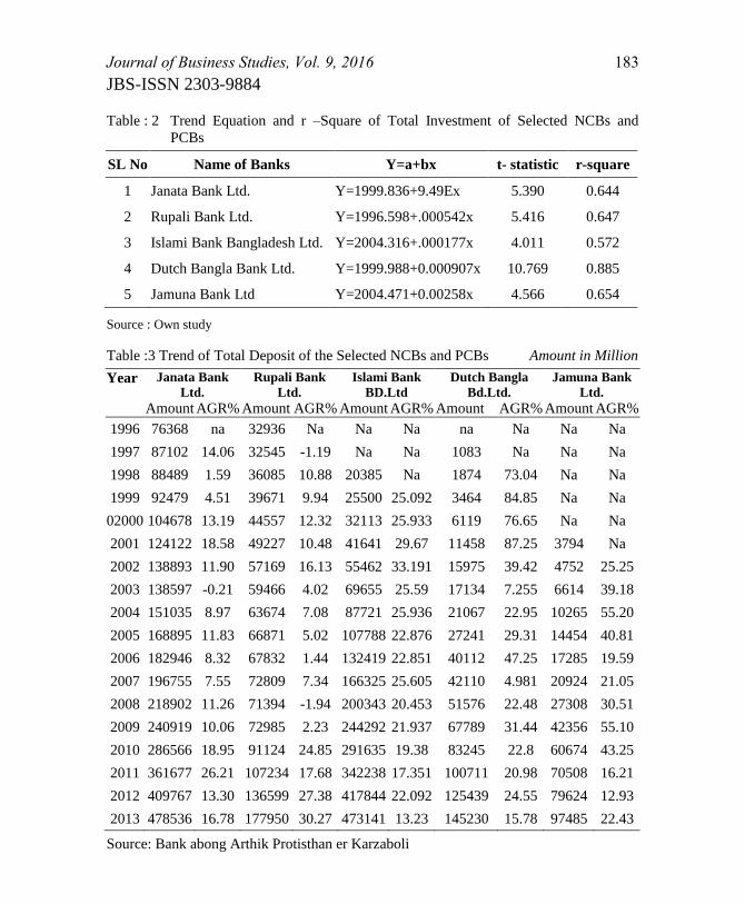
Journal of Business Studies, Vol. 9, 2016 183
JBS-ISSN 2303-9884
Table : 2 Trend Equation and r –Square of Total Investment of Selected NCBs and
PCBs
SL No Name of Banks Y=a+bx t- statistic r-square
1 Janata Bank Ltd. Y=1999.836+9.49Ex 5.390 0.644
2 Rupali Bank Ltd. Y=1996.598+.000542x 5.416 0.647
3 Islami Bank Bangladesh Ltd. Y=2004.316+.000177x 4.011 0.572
4 Dutch Bangla Bank Ltd. Y=1999.988+0.000907x 10.769 0.885
5 Jamuna Bank Ltd Y=2004.471+0.00258x 4.566 0.654
Source : Own study
Table :3 Trend of Total Deposit of the Selected NCBs and PCBs Amount in Million
Year Janata Bank
Ltd.
Rupali Bank
Ltd.
Islami Bank
BD.Ltd
Dutch Bangla
Bd.Ltd.
Jamuna Bank
Ltd.
Amount AGR% Amount AGR% Amount AGR% Amount AGR% Amount AGR%
1996 76368 na 32936 Na Na Na na Na Na Na
1997 87102 14.06 32545 -1.19 Na Na 1083 Na Na Na
1998 88489 1.59 36085 10.88 20385 Na 1874 73.04 Na Na
1999 92479 4.51 39671 9.94 25500 25.092 3464 84.85 Na Na
02000 104678 13.19 44557 12.32 32113 25.933 6119 76.65 Na Na
2001 124122 18.58 49227 10.48 41641 29.67 11458 87.25 3794 Na
2002 138893 11.90 57169 16.13 55462 33.191 15975 39.42 4752 25.25
2003 138597 -0.21 59466 4.02 69655 25.59 17134 7.255 6614 39.18
2004 151035 8.97 63674 7.08 87721 25.936 21067 22.95 10265 55.20
2005 168895 11.83 66871 5.02 107788 22.876 27241 29.31 14454 40.81
2006 182946 8.32 67832 1.44 132419 22.851 40112 47.25 17285 19.59
2007 196755 7.55 72809 7.34 166325 25.605 42110 4.981 20924 21.05
2008 218902 11.26 71394 -1.94 200343 20.453 51576 22.48 27308 30.51
2009 240919 10.06 72985 2.23 244292 21.937 67789 31.44 42356 55.10
2010 286566 18.95 91124 24.85 291635 19.38 83245 22.8 60674 43.25
2011 361677 26.21 107234 17.68 342238 17.351 100711 20.98 70508 16.21
2012 409767 13.30 136599 27.38 417844 22.092 125439 24.55 79624 12.93
2013 478536 16.78 177950 30.27 473141 13.23 145230 15.78 97485 22.43
Source: Bank abong Arthik Protisthan er Karzaboli

184 Journal of Business Studies, Vol. 9, 2016
JBS-ISSN 2303-9884
Table : 4 Trend Equation and r –Square of Total Deposit of Selected NCBs and PCBs
SL No Name of Banks Y=a+bx t-statistic r-square
1 Janata Bank Ltd. Y=1996.249+4.19Ex 9.5617 0.851
2 Rupali Bank Ltd. Y=1995.623+0.000125x 7.473 0.777
3 Islami Bank Bangladesh Ltd. Y=2000.237+3.11Ex 11.5377 0.904
4 Dutch Bangla Bank Ltd. Y=2000.305+0.000105x 10.030 0.870
5 Jamuna Bank Ltd Y=2002.938+0.000116x 9.763 0.896
Source : Own Study
Table : 5 Trend of Branches of the Selected NCBs and PCBs Amount in Million
Year Janata Bank
Ltd.
Rupali Bank
Ltd.
Islami Bank
BD.Ltd
Dutch Bangla
Bd.Ltd. Jamuna Bank
Ltd.
Amount AGR% Amount AGR% Amount AGR% Amount AGR% Amount AGR%
1996 897 Na 516 Na 95 Na Na Na Na Na
1997 897 0 516 0 100 5.26 1 Na Na Na
1998 897 0 514 -0.39 105 5.00 4 300 Na Na
1999 898 0.11 512 -0.39 110 4.76 6 50 Na Na
2000 898 0.00 512 0 116 5.45 9 50 Na Na
2001 900 0.22 514 0.39 121 4.31 11 22.222 3 Na
2002 870 -3.33 506 -1.56 128 5.79 17 54.545 8 166.7
2003 847 -2.64 493 -2.57 141 10.16 17 0 15 87.5
2004 847 0 493 0 151 7.09 19 11.765 19 26.7
2005 847 0 492 -0.20 169 11.92 28 47.368 23 21.1
2006 848 0.12 492 0 176 4.14 39 39.286 27 17.4
2007 848 0 492 0 186 5.68 49 25.641 35 29.6
2008 849 0.12 492 0 196 5.38 64 30.612 39 11.4
2009 851 0.24 492 0 231 17.86 79 23.438 54 38.5
2010 861 1.18 492 0 251 8.66 96 21.519 66 22.2
2011 873 1.39 503 2.24 266 5.98 111 15.625 73 10.6
2012 888 1.72 506 0.60 276 3.76 126 13.514 83 13.7
2013 893 0.56 532 5.13 286 3.62 136 7.93 91 9.63
Source: Bank abong Arthik Protisthan er Karzaboli

Journal of Business Studies, Vol. 9, 2016 185
JBS-ISSN 2303-9884
Table : 6 Trend Equation and r –Square of Branches of Selected NCBs and PCBs
SL No Name of Banks Y=a+bx t-statistic r-square
1 Janata Bank Ltd. Y=2093.982-0.102532x -1.946 0.1914
2 Rupali Bank Ltd. Y=2069.520-0.129052x -1.230 0.0864
3 Islami Bank Bangladesh Ltd. Y=1990.663+0.08024x 17.932 0.9526
4 Dutch Bangla Bank Ltd. Y=1999.995+0.10479x 11.4873 0.897
5 Jamuna Bank Ltd Y= 2001.614+0.13063x 18.5366 0.968
Source : Own study
Table: 7 Trend of Operating Profit of the Selected NCBs and PCBs Amount in Million
Year Janata Bank
Ltd.
Rupali Bank
Ltd.
Islami Bank
BD.Ltd
Dutch Bangla
Bd.Ltd.
Jamuna Bank
Ltd.
Amount AGR% Amount AGR% Amount AGR% Amount AGR% Amount AGR%
1996 947 371 284 Na Na
1997 1100 16.16 144 -61.19 243 -14.44 9 Na Na
1998 34 -96.91 -71 -149.31 148 -39.09 21 133.33 Na Na
1999 240 605.88 -308 333.80 167 12.84 86 309.52 Na Na
2000 831 246.25 102 -133.12 330 97.60 239 177.91 Na Na
2001 1597 92.18 287 181.37 577 74.85 397 66.11 0 Na
2002 1231 -22.92 622 116.72 994 72.27 423 6.55 15 Na
2003 2121 72.30 553 -11.09 803 -19.22 454 7.33 129 760
2004 2313 9.05 513 -7.23 1225 52.55 632 39.21 308 138.76
2005 3301 42.72 811 58.09 2163 76.57 940 48.73 420 36.36
2006 4213 27.63 255 -68.56 2908 34.44 1080 14.89 701 66.90
2007 4962 17.78 363 42.35 3781 30.02 1438 33.15 824 17.55
2008 7003 41.13 1145 215.43 6834 80.75 1936 34.63 1041 26.33
2009 8579 22.50 2099 83.32 6518 -4.62 2695 39.20 1914 83.86
2010 12108 41.14 2447 16.58 8455 29.72 4197 55.73 2406 25.71
2011 16013 32.25 3603 47.24 12731 50.57 4779 13.87 2807 16.67
2012 14734 -7.99 3674 1.97 15608 22.60 5206 8.93 3160 12.58
2013 12127 -17.69 1803 -50.93 14104 -9.64 2954 -43.25 4584 45.06
Source: Bank abong Arthik Protisthan er Karzaboli

186 Journal of Business Studies, Vol. 9, 2016
JBS-ISSN 2303-9884
Table : 8 Trend Equation and r –Square of Operating Profit of Selected NCBs and
PCBs
SL No Name of Banks Y=a+bx t-statistic r-square
1 Janata Bank Ltd. Y= 1999.762+0.00091x 8.421 0.815
2 Rupali Bank Ltd. Y=2000.835+0.00358x 5.525 0.656
3 Islami Bank Bangladesh Ltd. Y= 2000.542+0.00091x 7.848 0.793
4 Dutch Bangla Bank Ltd. Y= 2000.82+0.002583x 7.397 0.784
5 Jamuna Bank Ltd Y= 200.431+0.002534x 9.1968 0.884
Source : Own Study
Table :9 Trend of Total Manpower of the Selected NCBs and PCBs Amount in Million
Year
Janata Bank
Ltd.
Rupali Bank
Ltd.
Islami Bank
BD. Ltd
Dutch Bangla
Bd. Ltd.
Jamuna Bank
Ltd.
Amount AGR% Amount AGR% Amount AGR% Amount AGR% Amount AGR%
1996 17351 Na 6179 Na 1774 Na Na
1997 17113 -1.37 6007 -2.78 1903 7.27 55 Na Na
1998 17451 1.98 6084 1.28 2171 14.08 99 80 Na Na
1999 17138 -1.79 5885 -3.27 2302 6.03 176 77.78 Na Na
2000 16947 -1.11 5778 -1.82 2685 16.64 248 40.91 115
2001 16692 -1.50 5824 0.80 3060 13.97 317 27.82 140 21.739
2002 16330 -2.17 5628 -3.37 3297 7.75 409 29.02 153 9.29
2003 15993 -2.06 5412 -3.84 3752 13.80 437 6.85 253 65.359
2004 15705 -1.80 5225 -3.46 4261 13.57 431 -1.37 314 24.111
2005 15321 -2.45 5008 -4.15 5884 38.09 548 27.15 438 39.49
2006 14772 -3.58 4753 -5.09 7133 21.23 684 24.82 670 52.968
2007 13860 -6.17 4430 -6.80 8083 13.32 789 15.35 861 28.507
2008 13379 -3.47 4269 -3.63 9397 16.26 1229 55.77 938 8.9431
2009 13122 -1.92 4529 6.09 9588 2.03 1785 45.24 1215 29.531
2010 12826 -2.26 4503 -0.57 10349 7.94 2763 54.79 1511 24.362
2011 15020 17.11 4982 10.64 11465 10.78 4015 45.31 1786 18.2
2012 15071 0.34 5645 13.31 12188 6.31 5268 31.21 2050 14.782
2013 15370 1.98 5669 0.42 12980 6.49 4666 -11.42 2206 7.60
Source: Bank abong Arthik Protisthan er Karzaboli
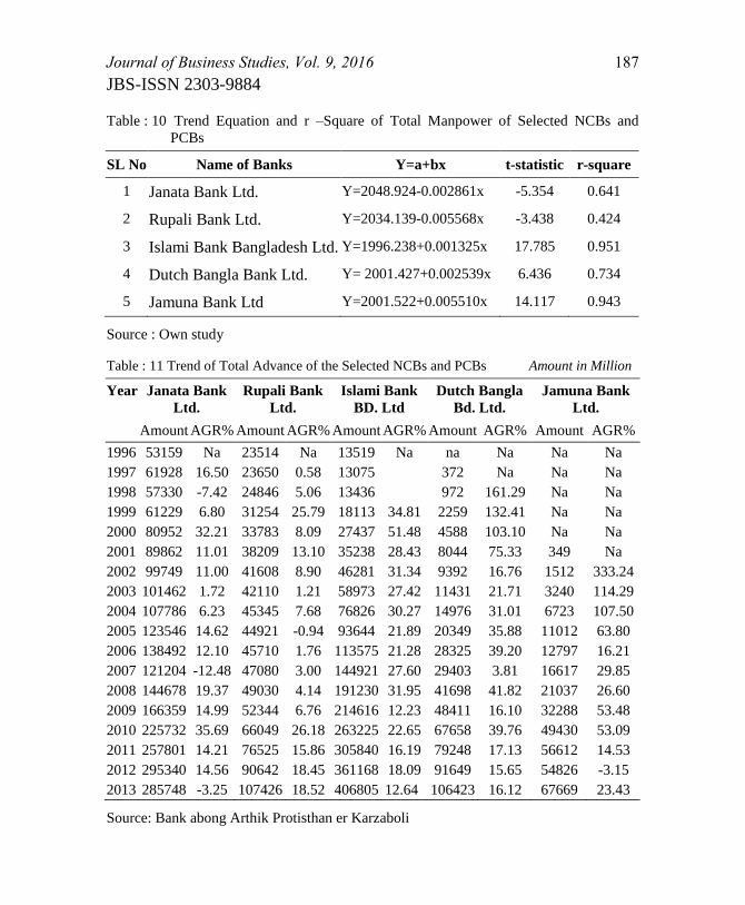
Journal of Business Studies, Vol. 9, 2016 187
JBS-ISSN 2303-9884
Table : 10 Trend Equation and r –Square of Total Manpower of Selected NCBs and
PCBs
SL No Name of Banks Y=a+bx t-statistic r-square
1 Janata Bank Ltd. Y=2048.924-0.002861x -5.354 0.641
2 Rupali Bank Ltd. Y=2034.139-0.005568x -3.438 0.424
3 Islami Bank Bangladesh Ltd. Y=1996.238+0.001325x 17.785 0.951
4 Dutch Bangla Bank Ltd. Y= 2001.427+0.002539x 6.436 0.734
5 Jamuna Bank Ltd Y=2001.522+0.005510x 14.117 0.943
Source : Own study
Table : 11 Trend of Total Advance of the Selected NCBs and PCBs Amount in Million
Year Janata Bank
Ltd.
Rupali Bank
Ltd.
Islami Bank
BD. Ltd
Dutch Bangla
Bd. Ltd.
Jamuna Bank
Ltd.
Amount AGR% Amount AGR% Amount AGR% Amount AGR% Amount AGR%
1996 53159 Na 23514 Na 13519 Na na Na Na Na
1997 61928 16.50 23650 0.58 13075 372 Na Na Na
1998 57330 -7.42 24846 5.06 13436 972 161.29 Na Na
1999 61229 6.80 31254 25.79 18113 34.81 2259 132.41 Na Na
2000 80952 32.21 33783 8.09 27437 51.48 4588 103.10 Na Na
2001 89862 11.01 38209 13.10 35238 28.43 8044 75.33 349 Na
2002 99749 11.00 41608 8.90 46281 31.34 9392 16.76 1512 333.24
2003 101462 1.72 42110 1.21 58973 27.42 11431 21.71 3240 114.29
2004 107786 6.23 45345 7.68 76826 30.27 14976 31.01 6723 107.50
2005 123546 14.62 44921 -0.94 93644 21.89 20349 35.88 11012 63.80
2006 138492 12.10 45710 1.76 113575 21.28 28325 39.20 12797 16.21
2007 121204 -12.48 47080 3.00 144921 27.60 29403 3.81 16617 29.85
2008 144678 19.37 49030 4.14 191230 31.95 41698 41.82 21037 26.60
2009 166359 14.99 52344 6.76 214616 12.23 48411 16.10 32288 53.48
2010 225732 35.69 66049 26.18 263225 22.65 67658 39.76 49430 53.09
2011 257801 14.21 76525 15.86 305840 16.19 79248 17.13 56612 14.53
2012 295340 14.56 90642 18.45 361168 18.09 91649 15.65 54826 -3.15
2013 285748 -3.25 107426 18.52 406805 12.64 106423 16.12 67669 23.43
Source: Bank abong Arthik Protisthan er Karzaboli
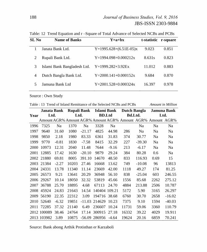
188 Journal of Business Studies, Vol. 9, 2016
JBS-ISSN 2303-9884
Table: 12 Trend Equation and r –Square of Total Advance of Selected NCBs and PCBs
SL No Name of Banks Y=a+bx t-statistic r-square
1 Janata Bank Ltd. Y=1995.628+(6.51E-05)x 9.023 0.851
2 Rupali Bank Ltd. Y=1994.098+0.000212x 8.631s 0.823
3 Islami Bank Bangladesh Ltd. Y=1999.282+3.92Ex 11.012 0.883
4 Dutch Bangla Bank Ltd. Y=2000.141+0.000152x 9.684 0.870
5 Jamuna Bank Ltd Y=2001.528+0.000324x 16.397 0.978
Source : Own Study
Table : 13 Trend of Inland Remittance of the Selected NCBs and PCBs Amount in Million
Year
Janata Bank
Ltd.
Rupali Bank
Ltd.
Islami Bank
BD.Ltd
Dutch Bangla
Bd.Ltd.
Jamuna Bank
Ltd.
Amount AGR% Amount AGR% Amount AGR% Amount AGR% Amount AGR%
1996 7325 Na 1370 Na 3328 Na Na Na Na
1997 9640 31.60 1080 -21.17 4825 44.98 286 Na Na Na
1998 9850 2.18 1980 83.33 6361 31.83 374 30.77 Na Na
1999 9770 -0.81 1830 -7.58 8415 32.29 227 -39.30 Na Na
2000 10973 12.31 2040 11.48 7644 -9.16 213 -6.17 Na Na
2001 12885 17.42 1630 -20.10 9879 29.24 384 80.28 0.6 Na
2002 21880 69.81 8005 391.10 14670 48.50 833 116.93 0.69 15
2003 21384 -2.27 10203 27.46 16668 13.62 749 -10.08 96 13813
2004 24331 13.78 11340 11.14 23669 42.00 1118 49.27 174 81.25
2005 26573 9.21 13641 20.29 36948 56.10 838 -25.04 603 246.55
2006 29267 10.14 18050 32.32 53819 45.66 1556 85.68 2262 275.12
2007 36788 25.70 18895 4.68 67113 24.70 4884 213.88 2506 10.787
2008 45924 24.83 21643 14.54 140404 109.21 5172 5.90 3165 26.297
2009 56190 22.35 22312 3.09 194716 38.68 6760 30.70 2658 -16.02
2010 52640 -6.32 19851 -11.03 214629 10.23 7375 9.10 1594 -40.03
2011 72285 37.32 21140 6.49 236607 10.24 11731 59.06 3360 110.79
2012 100089 38.46 24764 17.14 300915 27.18 16332 39.22 4029 19.911
2013 103982 3.89 10875 -56.09 286956 -4.64 19624 20.16 6859 70.241
Source: Bank abong Arthik Protisthan er Karzaboli
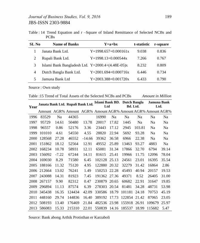
Journal of Business Studies, Vol. 9, 2016 189
JBS-ISSN 2303-9884
Table : 14 Trend Equation and r –Square of Inland Remittance of Selected NCBs and
PCBs
SL No Name of Banks Y=a+bx t-statistic r-square
1 Janata Bank Ltd. Y=1998.657+0.000161x 9.038 0.836
2 Rupali Bank Ltd. Y=1998.13+0.000544x 7.266 0.767
3 Islami Bank Bangladesh Ltd. Y=2000.4+(4.48E-05)x 8.232 0.809
4 Dutch Bangla Bank Ltd. Y=2001.694+0.000716x 6.446 0.734
5 Jamuna Bank Ltd Y=2003.388+0.001720x 6.433 0.790
Source : Own study
Table :15 Trend of Total Assets of the Selected NCBs and PCBs Amount in Million
Year Janata Bank Ltd. Rupali Bank Ltd.
Islami Bank BD.
Ltd
Dutch Bangla
Bd. Ltd.
Jamuna Bank
Ltd.
Amount AGR% Amount AGR% Amount AGR% Amount AGR% Amount AGR%
1996 83529 Na 44365 16990 Na Na Na Na Na
1997 95729 14.61 50480 13.78 20017 17.82 1445 Na Na Na
1998 96557 0.86 52176 3.36 23443 17.12 2945 103.81 Na Na
1999 101010 4.61 54550 4.55 28820 22.94 5692 93.28 Na Na
2000 128568 27.28 46552 -14.66 39362 36.58 6966 22.38 Na Na
2001 151862 18.12 52564 12.91 49552 25.89 13463 93.27 4883 Na
2002 168234 10.78 58931 12.11 65081 31.34 17866 32.70 6794 39.14
2003 156092 -7.22 67244 14.11 81615 25.41 19966 11.75 12096 78.04
2004 169030 8.29 71580 6.45 102128 25.13 24561 23.01 16395 35.54
2005 188166 11.32 75120 4.95 122880 20.32 32279 31.42 16864 2.86
2006 212664 13.02 76241 1.49 150253 22.28 45493 40.94 20157 19.53
2007 243088 14.31 81923 7.45 191362 27.36 49371 8.52 26405 31.00
2008 267157 9.90 82312 0.47 230879 20.65 60682 22.91 31647 19.85
2009 296894 11.13 87574 6.39 278303 20.54 81481 34.28 48731 53.98
2010 345438 16.35 124434 42.09 330586 18.79 101181 24.18 70753 45.19
2011 448160 29.74 144836 16.40 389192 17.73 122854 21.42 87065 23.05
2012 508193 13.40 176469 21.84 482536 23.98 155918 26.91 109679 25.97
2013 586083 15.33 215310 22.01 550839 14.16 185537 18.99 115682 5.47
Source: Bank abong Arthik Protisthan er Karzaboli
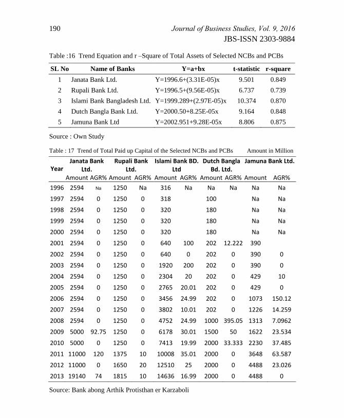
190 Journal of Business Studies, Vol. 9, 2016
JBS-ISSN 2303-9884
Table :16 Trend Equation and r –Square of Total Assets of Selected NCBs and PCBs
SL No Name of Banks Y=a+bx t-statistic r-square
1 Janata Bank Ltd. Y=1996.6+(3.31E-05)x 9.501 0.849
2 Rupali Bank Ltd. Y=1996.5+(9.56E-05)x 6.737 0.739
3 Islami Bank Bangladesh Ltd. Y=1999.289+(2.97E-05)x 10.374 0.870
4 Dutch Bangla Bank Ltd. Y=2000.50+8.25E-05x 9.164 0.848
5 Jamuna Bank Ltd Y=2002.951+9.28E-05x 8.806 0.875
Source : Own Study
Table : 17 Trend of Total Paid up Capital of the Selected NCBs and PCBs Amount in Million
Year Janata Bank
Ltd. Rupali Bank
Ltd. Islami Bank BD.
Ltd Dutch Bangla
Bd. Ltd. Jamuna Bank Ltd.
Amount AGR% Amount AGR% Amount AGR% Amount AGR% Amount AGR%
1996 2594 Na 1250 Na 316 Na Na Na Na Na
1997 2594 0 1250 0 318 100 Na Na
1998 2594 0 1250 0 320 180 Na Na
1999 2594 0 1250 0 320 180 Na Na
2000 2594 0 1250 0 320 180 Na Na
2001 2594 0 1250 0 640 100 202 12.222 390
2002 2594 0 1250 0 640 0 202 0 390 0
2003 2594 0 1250 0 1920 200 202 0 390 0
2004 2594 0 1250 0 2304 20 202 0 429 10
2005 2594 0 1250 0 2765 20.01 202 0 429 0
2006 2594 0 1250 0 3456 24.99 202 0 1073 150.12
2007 2594 0 1250 0 3802 10.01 202 0 1226 14.259
2008 2594 0 1250 0 4752 24.99 1000 395.05 1313 7.0962
2009 5000 92.75 1250 0 6178 30.01 1500 50 1622 23.534
2010 5000 0 1250 0 7413 19.99 2000 33.333 2230 37.485
2011 11000 120 1375 10 10008 35.01 2000 0 3648 63.587
2012 11000 0 1650 20 12510 25 2000 0 4488 23.026
2013 19140 74 1815 10 14636 16.99 2000 0 4488 0
Source: Bank abong Arthik Protisthan er Karzaboli

Journal of Business Studies, Vol. 9, 2016 191
JBS-ISSN 2303-9884
Table : 18 Trend Equation and r –Square of Total Paid Up Capital of Selected NCBs and
PCBs
SL No Name of Banks Y=a+bx t-statistic r-square
1 Janata Bank Ltd. Y=2000.649+0.000817x 3.812 0.476
2 Rupali Bank Ltd. Y=1978.17+0.020089x 2.981 0.357
3 Islami Bank Bangladesh Ltd. Y=2000.127+0.001084x 8.524 0.819
4 Dutch Bangla Bank Ltd. Y=2001.04+0.005355x 6.353 0.729
5 Jamuna Bank Ltd Y=2003.090+0.002299x 7.4686 0.835
Source : Own study
Table 19 Trend of Total Authorized Capital of the Selected NCBs and PCBs Amount in Mill.
Year Janata Bank
Ltd.
Rupali Bank
Ltd.
Islami Bank
BD. Ltd
Dutch Bangla
Bd. Ltd.
Jamuna Bank
Ltd.
Amount AGR% Amount AGR% Amount AGR% Amount AGR% Amount AGR%
1996 8000 Na 7000 Na 500 Na Na Na Na Na
1997 8000 7000 500 400 Na Na Na
1998 8000 7000 500 400 Na Na Na
1999 8000 7000 500 400 Na Na Na
2000 8000 7000 1000 400 Na Na Na
2001 8000 0 7000 0 1000 0 400 0 1600 Na
2002 8000 0 7000 0 1000 0 400 0 1600 0
2003 8000 0 7000 0 3000 200 400 0 1600 0
2004 8000 0 7000 0 3000 0 400 0 1600 0
2005 8000 0 7000 0 5000 66.667 400 0 1600 0
2006 8000 0 7000 0 5000 0 400 0 1600 0
2007 8000 0 7000 0 5000 0 400 0 4000 150
2008 8000 0 7000 0 10000 100 1000 150 4000 0
2009 20000 150 7000 0 10000 0 1000 0 4000 0
2010 20000 0 7000 0 10000 0 4000 300 10000 150
2011 20000 0 7000 0 20000 100 4000 0 10000 0
2012 20000 0 7000 0 20000 0 4000 0 10000 0
2013 20000 7000 0 20000 0 4000 0 10000 0
Source: Bank abong Arthik Protisthan er Karzaboli

192 Journal of Business Studies, Vol. 9, 2016
JBS-ISSN 2303-9884
Table: 20 Trend Equation and r –Square of Total Authorized Capital of Selected NCBs
and PCBs
SL No Name of Banks Y=a+bx t-statistic r-square
1 Janata Bank Ltd. Y=1996.333+0.000708x 4.210 0.541
2 Rupali Bank Ltd. - - -
3 Islami Bank Bangladesh Ltd. Y=2000.122+0.000679x 8.230 0.808
4 Dutch Bangla Bank Ltd. Y=2000.630+0.002557x 4.874 0.612
5 Jamuna Bank Ltd Y=2002.623+0.000924x 6.717 0.803
Source : Own Study
Table : 21 Trend of Total Import of the Selected NCBs and PCBs Amount in Million
Year
Janata Bank
Ltd.
Rupali Bank
Ltd.
Islami Bank
BD.Ltd
Dutch Bangla
Bd.Ltd.
Jamuna Bank
Ltd.
Amount AGR% Amount AGR% Amount AGR% Amount AGR% Amount AGR%
1996 37860 na 12312 Na 17875 Na na na Na Na
1997 36938 -2.44 14500 17.77 17370 -2.83 598 na Na Na
1998 45401 22.91 21360 47.31 20238 16.51 1634 173.24 Na Na
1999 43250 -4.74 13722 -35.76 20396 0.78 4413 170.07 Na Na
2000 48005 10.99 21120 53.91 16889 -17.19 8329 88.74 Na Na
2001 54666 13.88 20637 -2.29 25907 53.40 11215 34.65 125 Na
2002 58910 7.76 17044 -17.41 33788 30.42 11856 5.72 1449 1059.2
2003 60476 2.66 19849 16.46 46237 36.84 17550 48.03 3081 112.63
2004 74920 23.88 24424 23.05 59804 29.34 25974 48.00 7923 157.16
2005 72912 -2.68 21654 -11.34 74525 24.62 26029 0.21 11152 40.755
2006 128809 76.66 14840 -31.47 96870 29.98 32068 23.20 15458 38.612
2007 84065 -34.74 19857 33.81 103293 6.63 35667 11.22 22192 43.563
2008 129413 53.94 20590 3.69 168329 62.96 43999 23.36 30312 36.59
2009 118525 -8.41 55033 167.28 161230 -4.22 53089 20.66 46685 54.015
2010 183744 55.03 60245 9.47 246281 52.75 87663 65.12 61035 30.738
2011 197285 7.37 69263 14.97 301207 22.30 83434 -4.82 55907 -8.402
2012 188283 -4.56 45108 -34.87 284587 -5.52 108878 30.50 57705 3.2161
2013 176671 -6.17 65165 44.46 285890 0.46 108259 -0.57 52751 -8.58
Source: Bank abong Arthik Protisthan er Karzaboli
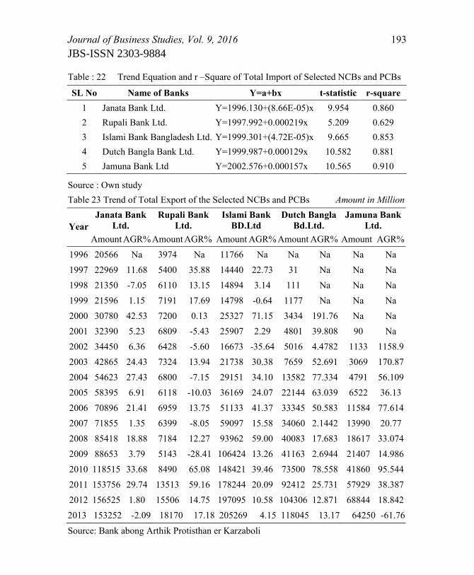
Journal of Business Studies, Vol. 9, 2016 193
JBS-ISSN 2303-9884
Table : 22 Trend Equation and r –Square of Total Import of Selected NCBs and PCBs
SL No Name of Banks Y=a+bx t-statistic r-square
1 Janata Bank Ltd. Y=1996.130+(8.66E-05)x 9.954 0.860
2 Rupali Bank Ltd. Y=1997.992+0.000219x 5.209 0.629
3 Islami Bank Bangladesh Ltd. Y=1999.301+(4.72E-05)x 9.665 0.853
4 Dutch Bangla Bank Ltd. Y=1999.987+0.000129x 10.582 0.881
5 Jamuna Bank Ltd Y=2002.576+0.000157x 10.565 0.910
Source : Own study
Table 23 Trend of Total Export of the Selected NCBs and PCBs Amount in Million
Year
Janata Bank
Ltd.
Rupali Bank
Ltd.
Islami Bank
BD.Ltd
Dutch Bangla
Bd.Ltd.
Jamuna Bank
Ltd.
Amount AGR% Amount AGR% Amount AGR% Amount AGR% Amount AGR%
1996 20566 Na 3974 Na 11766 Na Na Na Na Na
1997 22969 11.68 5400 35.88 14440 22.73 31 Na Na Na
1998 21350 -7.05 6110 13.15 14894 3.14 111 Na Na Na
1999 21596 1.15 7191 17.69 14798 -0.64 1177 Na Na Na
2000 30780 42.53 7200 0.13 25327 71.15 3434 191.76 Na Na
2001 32390 5.23 6809 -5.43 25907 2.29 4801 39.808 90 Na
2002 34450 6.36 6428 -5.60 16673 -35.64 5016 4.4782 1133 1158.9
2003 42865 24.43 7324 13.94 21738 30.38 7659 52.691 3069 170.87
2004 54623 27.43 6800 -7.15 29151 34.10 13582 77.334 4791 56.109
2005 58395 6.91 6118 -10.03 36169 24.07 22144 63.039 6522 36.13
2006 70896 21.41 6959 13.75 51133 41.37 33345 50.583 11584 77.614
2007 71855 1.35 6399 -8.05 59097 15.58 34060 2.1442 13990 20.77
2008 85418 18.88 7184 12.27 93962 59.00 40083 17.683 18617 33.074
2009 88653 3.79 5143 -28.41 106424 13.26 41163 2.6944 21407 14.986
2010 118515 33.68 8490 65.08 148421 39.46 73500 78.558 41860 95.544
2011 153756 29.74 13513 59.16 178244 20.09 92412 25.731 57929 38.387
2012 156525 1.80 15506 14.75 197095 10.58 104306 12.871 68844 18.842
2013 153252 -2.09 18170 17.18 205269 4.15 118045 13.17 64250 -61.76
Source: Bank abong Arthik Protisthan er Karzaboli
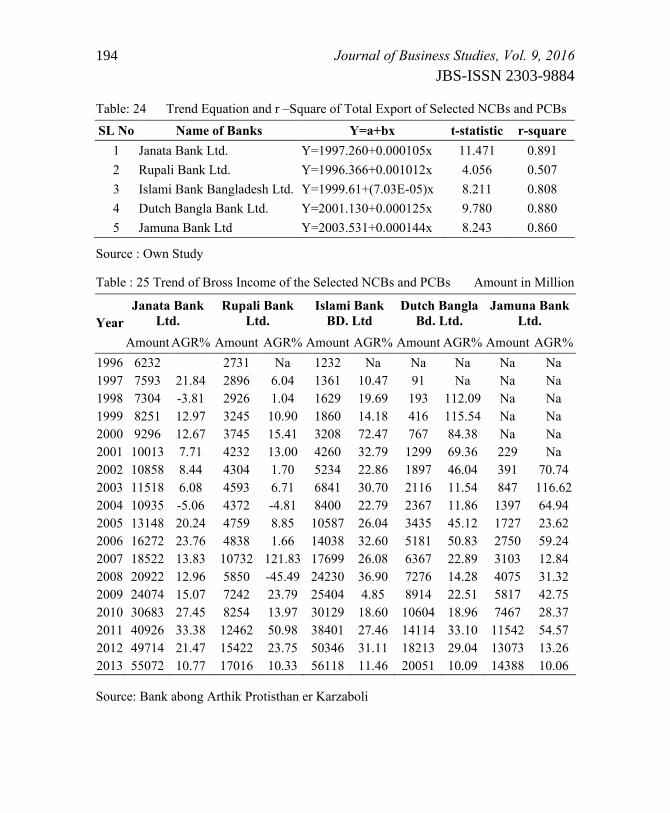
194 Journal of Business Studies, Vol. 9, 2016
JBS-ISSN 2303-9884
Table: 24 Trend Equation and r –Square of Total Export of Selected NCBs and PCBs
SL No Name of Banks Y=a+bx t-statistic r-square
1 Janata Bank Ltd. Y=1997.260+0.000105x 11.471 0.891
2 Rupali Bank Ltd. Y=1996.366+0.001012x 4.056 0.507
3 Islami Bank Bangladesh Ltd. Y=1999.61+(7.03E-05)x 8.211 0.808
4 Dutch Bangla Bank Ltd. Y=2001.130+0.000125x 9.780 0.880
5 Jamuna Bank Ltd Y=2003.531+0.000144x 8.243 0.860
Source : Own Study
Table : 25 Trend of Bross Income of the Selected NCBs and PCBs Amount in Million
Year
Janata Bank
Ltd.
Rupali Bank
Ltd.
Islami Bank
BD. Ltd
Dutch Bangla
Bd. Ltd.
Jamuna Bank
Ltd.
Amount AGR% Amount AGR% Amount AGR% Amount AGR% Amount AGR%
1996 6232 2731 Na 1232 Na Na Na Na Na
1997 7593 21.84 2896 6.04 1361 10.47 91 Na Na Na
1998 7304 -3.81 2926 1.04 1629 19.69 193 112.09 Na Na
1999 8251 12.97 3245 10.90 1860 14.18 416 115.54 Na Na
2000 9296 12.67 3745 15.41 3208 72.47 767 84.38 Na Na
2001 10013 7.71 4232 13.00 4260 32.79 1299 69.36 229 Na
2002 10858 8.44 4304 1.70 5234 22.86 1897 46.04 391 70.74
2003 11518 6.08 4593 6.71 6841 30.70 2116 11.54 847 116.62
2004 10935 -5.06 4372 -4.81 8400 22.79 2367 11.86 1397 64.94
2005 13148 20.24 4759 8.85 10587 26.04 3435 45.12 1727 23.62
2006 16272 23.76 4838 1.66 14038 32.60 5181 50.83 2750 59.24
2007 18522 13.83 10732 121.83 17699 26.08 6367 22.89 3103 12.84
2008 20922 12.96 5850 -45.49 24230 36.90 7276 14.28 4075 31.32
2009 24074 15.07 7242 23.79 25404 4.85 8914 22.51 5817 42.75
2010 30683 27.45 8254 13.97 30129 18.60 10604 18.96 7467 28.37
2011 40926 33.38 12462 50.98 38401 27.46 14114 33.10 11542 54.57
2012 49714 21.47 15422 23.75 50346 31.11 18213 29.04 13073 13.26
2013 55072 10.77 17016 10.33 56118 11.46 20051 10.09 14388 10.06
Source: Bank abong Arthik Protisthan er Karzaboli
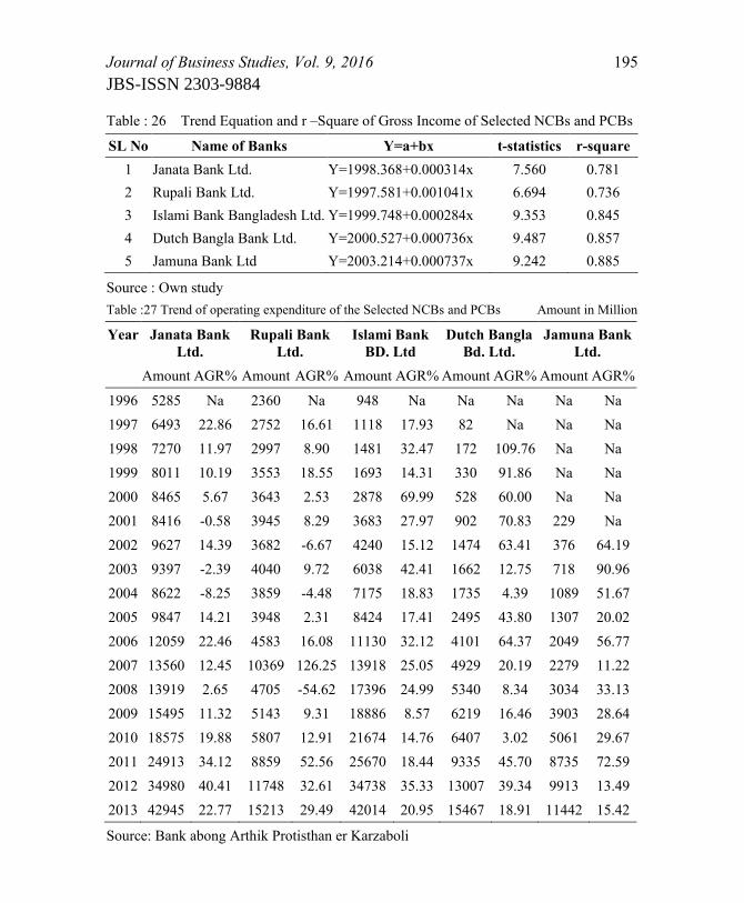
Journal of Business Studies, Vol. 9, 2016 195
JBS-ISSN 2303-9884
Table : 26 Trend Equation and r –Square of Gross Income of Selected NCBs and PCBs
SL No Name of Banks Y=a+bx t-statistics r-square
1 Janata Bank Ltd. Y=1998.368+0.000314x 7.560 0.781
2 Rupali Bank Ltd. Y=1997.581+0.001041x 6.694 0.736
3 Islami Bank Bangladesh Ltd. Y=1999.748+0.000284x 9.353 0.845
4 Dutch Bangla Bank Ltd. Y=2000.527+0.000736x 9.487 0.857
5 Jamuna Bank Ltd Y=2003.214+0.000737x 9.242 0.885
Source : Own study
Table :27 Trend of operating expenditure of the Selected NCBs and PCBs Amount in Million
Year Janata Bank
Ltd.
Rupali Bank
Ltd.
Islami Bank
BD. Ltd
Dutch Bangla
Bd. Ltd.
Jamuna Bank
Ltd.
Amount AGR% Amount AGR% Amount AGR% Amount AGR% Amount AGR%
1996 5285 Na 2360 Na 948 Na Na Na Na Na
1997 6493 22.86 2752 16.61 1118 17.93 82 Na Na Na
1998 7270 11.97 2997 8.90 1481 32.47 172 109.76 Na Na
1999 8011 10.19 3553 18.55 1693 14.31 330 91.86 Na Na
2000 8465 5.67 3643 2.53 2878 69.99 528 60.00 Na Na
2001 8416 -0.58 3945 8.29 3683 27.97 902 70.83 229 Na
2002 9627 14.39 3682 -6.67 4240 15.12 1474 63.41 376 64.19
2003 9397 -2.39 4040 9.72 6038 42.41 1662 12.75 718 90.96
2004 8622 -8.25 3859 -4.48 7175 18.83 1735 4.39 1089 51.67
2005 9847 14.21 3948 2.31 8424 17.41 2495 43.80 1307 20.02
2006 12059 22.46 4583 16.08 11130 32.12 4101 64.37 2049 56.77
2007 13560 12.45 10369 126.25 13918 25.05 4929 20.19 2279 11.22
2008 13919 2.65 4705 -54.62 17396 24.99 5340 8.34 3034 33.13
2009 15495 11.32 5143 9.31 18886 8.57 6219 16.46 3903 28.64
2010 18575 19.88 5807 12.91 21674 14.76 6407 3.02 5061 29.67
2011 24913 34.12 8859 52.56 25670 18.44 9335 45.70 8735 72.59
2012 34980 40.41 11748 32.61 34738 35.33 13007 39.34 9913 13.49
2013 42945 22.77 15213 29.49 42014 20.95 15467 18.91 11442 15.42
Source: Bank abong Arthik Protisthan er Karzaboli
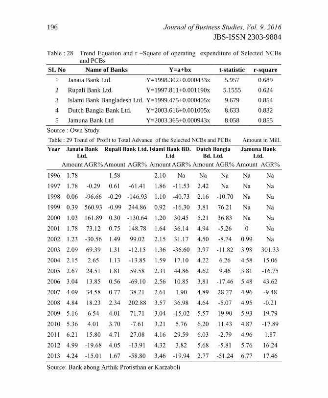
196 Journal of Business Studies, Vol. 9, 2016
JBS-ISSN 2303-9884
Table : 28 Trend Equation and r –Square of operating expenditure of Selected NCBs
and PCBs
SL No Name of Banks Y=a+bx t-statistic r-square
1 Janata Bank Ltd. Y=1998.302+0.000433x 5.957 0.689
2 Rupali Bank Ltd. Y=1997.811+0.001190x 5.1555 0.624
3 Islami Bank Bangladesh Ltd. Y=1999.475+0.000405x 9.679 0.854
4 Dutch Bangla Bank Ltd. Y=2003.616+0.001005x 8.633 0.832
5 Jamuna Bank Ltd Y=2003.365+0.000943x 8.058 0.855
Source : Own Study
Table : 29 Trend of Profit to Total Advance of the Selected NCBs and PCBs Amount in Mill.
Year Janata Bank
Ltd.
Rupali Bank Ltd. Islami Bank BD.
Ltd
Dutch Bangla
Bd. Ltd.
Jamuna Bank
Ltd.
Amount AGR% Amount AGR% Amount AGR% Amount AGR% Amount AGR%
1996 1.78 1.58 2.10 Na Na Na Na Na
1997 1.78 -0.29 0.61 -61.41 1.86 -11.53 2.42 Na Na Na
1998 0.06 -96.66 -0.29 -146.93 1.10 -40.73 2.16 -10.70 Na Na
1999 0.39 560.93 -0.99 244.86 0.92 -16.30 3.81 76.21 Na Na
2000 1.03 161.89 0.30 -130.64 1.20 30.45 5.21 36.83 Na Na
2001 1.78 73.12 0.75 148.78 1.64 36.14 4.94 -5.26 0 Na
2002 1.23 -30.56 1.49 99.02 2.15 31.17 4.50 -8.74 0.99 Na
2003 2.09 69.39 1.31 -12.15 1.36 -36.60 3.97 -11.82 3.98 301.33
2004 2.15 2.65 1.13 -13.85 1.59 17.10 4.22 6.26 4.58 15.06
2005 2.67 24.51 1.81 59.58 2.31 44.86 4.62 9.46 3.81 -16.75
2006 3.04 13.85 0.56 -69.10 2.56 10.85 3.81 -17.46 5.48 43.62
2007 4.09 34.58 0.77 38.21 2.61 1.90 4.89 28.27 4.96 -9.48
2008 4.84 18.23 2.34 202.88 3.57 36.98 4.64 -5.07 4.95 -0.21
2009 5.16 6.54 4.01 71.71 3.04 -15.02 5.57 19.90 5.93 19.79
2010 5.36 4.01 3.70 -7.61 3.21 5.76 6.20 11.43 4.87 -17.89
2011 6.21 15.80 4.71 27.08 4.16 29.59 6.03 -2.79 4.96 1.87
2012 4.99 -19.68 4.05 -13.91 4.32 3.82 5.68 -5.81 5.76 16.24
2013 4.24 -15.01 1.67 -58.80 3.46 -19.94 2.77 -51.24 6.77 17.46
Source: Bank abong Arthik Protisthan er Karzaboli
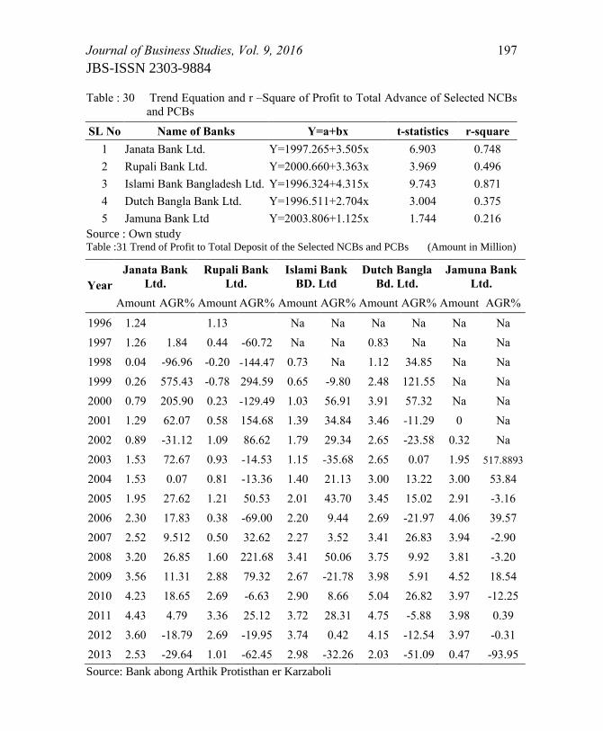
Journal of Business Studies, Vol. 9, 2016 197
JBS-ISSN 2303-9884
Table : 30 Trend Equation and r –Square of Profit to Total Advance of Selected NCBs
and PCBs
SL No Name of Banks Y=a+bx t-statistics r-square
1 Janata Bank Ltd. Y=1997.265+3.505x 6.903 0.748
2 Rupali Bank Ltd. Y=2000.660+3.363x 3.969 0.496
3 Islami Bank Bangladesh Ltd. Y=1996.324+4.315x 9.743 0.871
4 Dutch Bangla Bank Ltd. Y=1996.511+2.704x 3.004 0.375
5 Jamuna Bank Ltd Y=2003.806+1.125x 1.744 0.216
Source : Own study Table :31 Trend of Profit to Total Deposit of the Selected NCBs and PCBs (Amount in Million)
Year
Janata Bank
Ltd.
Rupali Bank
Ltd.
Islami Bank
BD. Ltd
Dutch Bangla
Bd. Ltd.
Jamuna Bank
Ltd.
Amount AGR% Amount AGR% Amount AGR% Amount AGR% Amount AGR%
1996 1.24 1.13 Na Na Na Na Na Na
1997 1.26 1.84 0.44 -60.72 Na Na 0.83 Na Na Na
1998 0.04 -96.96 -0.20 -144.47 0.73 Na 1.12 34.85 Na Na
1999 0.26 575.43 -0.78 294.59 0.65 -9.80 2.48 121.55 Na Na
2000 0.79 205.90 0.23 -129.49 1.03 56.91 3.91 57.32 Na Na
2001 1.29 62.07 0.58 154.68 1.39 34.84 3.46 -11.29 0 Na
2002 0.89 -31.12 1.09 86.62 1.79 29.34 2.65 -23.58 0.32 Na
2003 1.53 72.67 0.93 -14.53 1.15 -35.68 2.65 0.07 1.95 517.8893
2004 1.53 0.07 0.81 -13.36 1.40 21.13 3.00 13.22 3.00 53.84
2005 1.95 27.62 1.21 50.53 2.01 43.70 3.45 15.02 2.91 -3.16
2006 2.30 17.83 0.38 -69.00 2.20 9.44 2.69 -21.97 4.06 39.57
2007 2.52 9.512 0.50 32.62 2.27 3.52 3.41 26.83 3.94 -2.90
2008 3.20 26.85 1.60 221.68 3.41 50.06 3.75 9.92 3.81 -3.20
2009 3.56 11.31 2.88 79.32 2.67 -21.78 3.98 5.91 4.52 18.54
2010 4.23 18.65 2.69 -6.63 2.90 8.66 5.04 26.82 3.97 -12.25
2011 4.43 4.79 3.36 25.12 3.72 28.31 4.75 -5.88 3.98 0.39
2012 3.60 -18.79 2.69 -19.95 3.74 0.42 4.15 -12.54 3.97 -0.31
2013 2.53 -29.64 1.01 -62.45 2.98 -32.26 2.03 -51.09 0.47 -93.95
Source: Bank abong Arthik Protisthan er Karzaboli
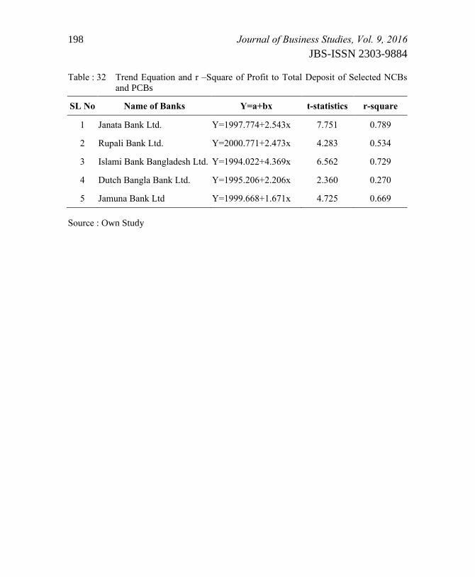
198 Journal of Business Studies, Vol. 9, 2016
JBS-ISSN 2303-9884
Table : 32 Trend Equation and r –Square of Profit to Total Deposit of Selected NCBs and PCBs
SL No Name of Banks Y=a+bx t-statistics r-square
1 Janata Bank Ltd. Y=1997.774+2.543x 7.751 0.789
2 Rupali Bank Ltd. Y=2000.771+2.473x 4.283 0.534
3 Islami Bank Bangladesh Ltd. Y=1994.022+4.369x 6.562 0.729
4 Dutch Bangla Bank Ltd. Y=1995.206+2.206x 2.360 0.270
5 Jamuna Bank Ltd Y=1999.668+1.671x 4.725 0.669
Source : Own Study
Journal of Business Studies, Vol. 9, 2016 199
JBS-ISSN 2303-9884
Succession Plan in Second or Subsequent Generation Family
Owned Firms in Bangladesh- a Study on Rajshahi Division Md. Shariful Islam1
Dr. Md. Amzad Hossain 2
Abstract
The study aims at exploring the existence and nature of succession plan in family
owned firms in Bangladesh. A survey has been conducted on second or
subsequent generation family owned firms in eight districts of Rajshahi Division.
Incumbents of 229 family owned firms have been interviewed using a
questionnaire. The study finds lack of existence of formal and written succession
plan. In most of the cases successors have not been identified. Siblings of the
incumbents play a major role in family owned firms. Incumbents mastermind the
succession plan, where exist, consulting with other family members. The study
also finds evidences of incomplete succession in a large number of cases even
after transfer of responsibilities of the firms to incumbents.
Keywords: Succession plan, family owned firms, generation of business
(I) Introduction
n the new global economy family owned firms play significantly
important role (Ibrahim, Soufani & Lam, 2001). Family owned firms
account for the majority of the whole businesses and contribute strongly in
the growth of the national economy of different countries (Nordqvist,
2005; Chrisman, Chua & Steier, 2005; Poutziouris, O‟Sullivan, &
Nicolescu, 1997; Gallo, 1995; Poza, 1995; Ibrahim & Ellis, 1994; Lank,
Owens, Martinez, Reidel, deVisscher, & Bruel, 1994). Succession is a
common phenomenon in every small and medium sized family owned
firm. It is considered as the most critical issue that is commonly faced by
the firms (Islam, Aleem, & Chowdhury, 2014; Ibrahim, Soufani, & Lam,
2001). Succession is very complex in family owned businesses (Miller,
Steier, & Le Breton-Miller, 2003; Lansberg, 1999; Dyer, 1986). Studies in
1 Associate Professor, Institute of Business Administration, University of Rajshahi Email: [email protected] 2 Professor, Department of Finance, University of Rajshahi
Email: [email protected]
I
200 Journal of Business Studies, Vol. 9, 2016
JBS-ISSN 2303-9884
the area of family business also show that such family owned firms strive
for continuity in ensuring competent leadership across generations for the
continuity of the business itself (Le Breton-Miller, Miller, & Steier, 2004).
Though the owners of family owned firms consider longevity of the
business as the most important concern (Nutek, 2004), evidence from
previous studies suggest that 30% of family businesses survive into the
second generation and only 10% or 15% make it to the third generation
(Aronoff, 1999; Kets de Vries 1993; Ward 1987). This higher rate of
failure of the family owned firms has become a concern of the researchers
(Aronoff, 1999; Lansberg, 1999; Handler 1990; Kepner, 1983). Therefore,
a proper succession planning and process is important in the sense that it
affords the family owned firms to select the most appropriate future
leaders to carry forward the business successfully (Islam, et al., 2014;
Ibrahim, McGuire, Ismail, & Dumas, 1999; Ward, 1987). Researchers
believe that there is need for formal succession plan in the family owned
firms and the plan should be long term (Kets de Vries, 1993; Ward &
Aronoff, 1992; Williams, 1992; Ward, 1987; Danco, 1982).
This paper is focused on presenting information related to succession plan
in family owned firms in Bangladesh. These information will be used in
future studies for advanced analysis to explore more specific issues related
to succession planning in family owned firms in Bangladesh.
(II) Method and Data
In this study a survey has been conducted on the family owned firms
located in eight districts under Rajshahi Division. Districts covered in this
research are (i) Rajshahi, (ii) Chapai Nawabgonj, (iii) Naogaon, (iv)
Natore, (v) Bogra, (vi) Jaipurhat, (vii) Pabna, and (viii) Sirajgonj. Family
owned firms from these districts have been selected using convenient
sampling method.
During selection of sample, the study considers factors such as control of
the family in the business in terms of ownership and generation(s)
involved. As there is no previously constructed database of family owned
firms in Bangladesh, the study did not have idea about the population. The
study collected list of the firms in each district from respective Chamber
of Commerce. Lists of firms, which are in operation at the BSCIC areas,
Journal of Business Studies, Vol. 9, 2016 201
JBS-ISSN 2303-9884
have also been collected from BSCIC offices. Afterwards the survey team
went outside BSCIC and prepared a sample frame of family owned firms
of the respective districts. In the first phase of the survey, the study
surveyed each of the enlisted firms to identify the family businesses.
During identifying family businesses, special care has been taken so that
the criteria of family business considered in the present study are fulfilled.
The study considers firms with the following criteria as family owned
firms:
(i) If the founder (or the founders of the same family, in case of multiple
founders) or descendant(s) of the founder (or founders of the same family)
or their spouses hold more than 50% of ownership of the business;
And/or
(ii) If the founder (or any of the founders, in case of multiple founders) or
descendant(s) of the founder(s) or their spouses serves as Chief Executive
Officer (CEO) or Chief of the Business (COB).
A formal questionnaire has been used for conducting the survey. The
questionnaire was tested through pilot survey conducted on 15 family
owned firms located in Rajshahi metropolitan city. Expert opinions have
also been invited after preparing the questionnaire. On the basis of pilot
survey and experts‟ opinions, several modifications and corrections have
been made. The revised and improved questionnaire has been used for
final survey.
From the first phase of the survey the study identifies 1489 family owned
firms out of which 865 firms fulfill criteria for the study and the family
business definition of the study. The study approached with the
questionnaire for data collection while 743 firms responded and 122
declined to participate in the interview. 514 family owned firms out of
total 743 are in first generation while the rest 229 family businesses are
identified as second generation or subsequent generations. The study has
approached with the interview questionnaire to those 229 second or
subsequent generation family owned firms with direct interviewing
method. Here, it should be noted that „generation‟ means the generation of
business, not the generation of family.
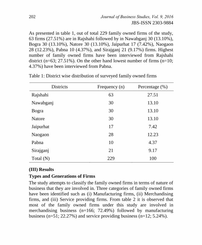
202 Journal of Business Studies, Vol. 9, 2016
JBS-ISSN 2303-9884
As presented in table 1, out of total 229 family owned firms of the study,
63 firms (27.51%) are in Rajshahi followed by in Nawabganj 30 (13.10%),
Bogra 30 (13.10%), Natore 30 (13.10%), Jaipurhat 17 (7.42%), Naogaon
28 (12.23%), Pabna 10 (4.37%), and Sirajganj 21 (9.17%) firms. Highest
number of family owned firms have been interviewed from Rajshahi
district (n=63; 27.51%). On the other hand lowest number of firms (n=10;
4.37%) have been interviewed from Pabna.
Table 1: District wise distribution of surveyed family owned firms
Districts Frequency (n) Percentage (%)
Rajshahi 63 27.51
Nawabganj 30 13.10
Bogra 30 13.10
Natore 30 13.10
Jaipurhat 17 7.42
Naogaon 28 12.23
Pabna 10 4.37
Sirajganj 21 9.17
Total (N) 229 100
(III) Results
Types and Generations of Firms
The study attempts to classify the family owned firms in terms of nature of
business that they are involved in. Three categories of family owned firms
have been identified such as (i) Manufacturing firms, (ii) Merchandising
firms, and (iii) Service providing firms. From table 2 it is observed that
most of the family owned firms under this study are involved in
merchandising business (n=166; 72.49%) followed by manufacturing
business (n=51; 22.27%) and service providing business (n=12; 5.24%).
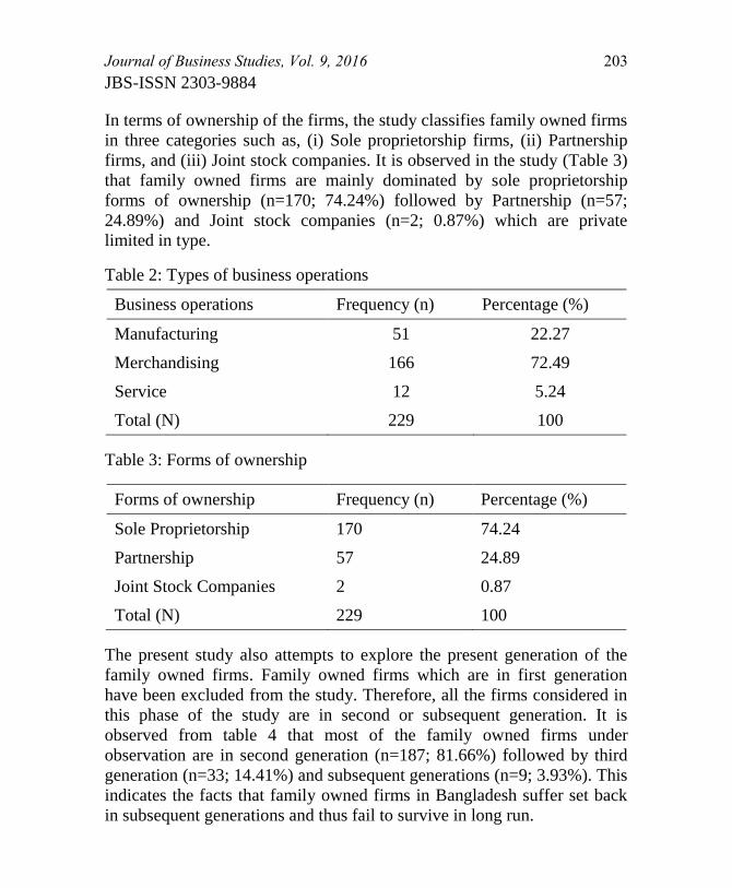
Journal of Business Studies, Vol. 9, 2016 203
JBS-ISSN 2303-9884
In terms of ownership of the firms, the study classifies family owned firms
in three categories such as, (i) Sole proprietorship firms, (ii) Partnership
firms, and (iii) Joint stock companies. It is observed in the study (Table 3)
that family owned firms are mainly dominated by sole proprietorship
forms of ownership (n=170; 74.24%) followed by Partnership (n=57;
24.89%) and Joint stock companies (n=2; 0.87%) which are private
limited in type.
Table 2: Types of business operations
Business operations Frequency (n) Percentage (%)
Manufacturing 51 22.27
Merchandising 166 72.49
Service 12 5.24
Total (N) 229 100
Table 3: Forms of ownership
Forms of ownership Frequency (n) Percentage (%)
Sole Proprietorship 170 74.24
Partnership 57 24.89
Joint Stock Companies 2 0.87
Total (N) 229 100
The present study also attempts to explore the present generation of the
family owned firms. Family owned firms which are in first generation
have been excluded from the study. Therefore, all the firms considered in
this phase of the study are in second or subsequent generation. It is
observed from table 4 that most of the family owned firms under
observation are in second generation (n=187; 81.66%) followed by third
generation (n=33; 14.41%) and subsequent generations (n=9; 3.93%). This
indicates the facts that family owned firms in Bangladesh suffer set back
in subsequent generations and thus fail to survive in long run.
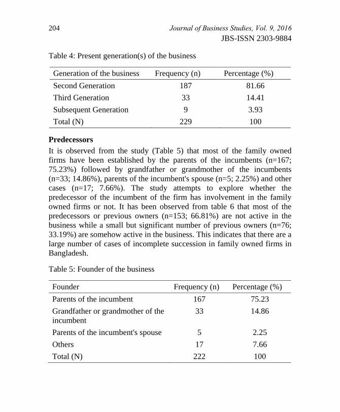
204 Journal of Business Studies, Vol. 9, 2016
JBS-ISSN 2303-9884
Table 4: Present generation(s) of the business
Generation of the business Frequency (n) Percentage (%)
Second Generation 187 81.66
Third Generation 33 14.41
Subsequent Generation 9 3.93
Total (N) 229 100
Predecessors
It is observed from the study (Table 5) that most of the family owned
firms have been established by the parents of the incumbents (n=167;
75.23%) followed by grandfather or grandmother of the incumbents
(n=33; 14.86%), parents of the incumbent's spouse (n=5; 2.25%) and other
cases (n=17; 7.66%). The study attempts to explore whether the
predecessor of the incumbent of the firm has involvement in the family
owned firms or not. It has been observed from table 6 that most of the
predecessors or previous owners (n=153; 66.81%) are not active in the
business while a small but significant number of previous owners (n=76;
33.19%) are somehow active in the business. This indicates that there are a
large number of cases of incomplete succession in family owned firms in
Bangladesh.
Table 5: Founder of the business
Founder Frequency (n) Percentage (%)
Parents of the incumbent 167 75.23
Grandfather or grandmother of the
incumbent
33 14.86
Parents of the incumbent's spouse 5 2.25
Others 17 7.66
Total (N) 222 100
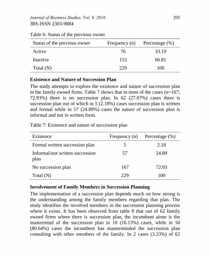
Journal of Business Studies, Vol. 9, 2016 205
JBS-ISSN 2303-9884
Table 6: Status of the previous owner
Status of the previous owner Frequency (n) Percentage (%)
Active 76 33.19
Inactive 153 66.81
Total (N) 229 100
Existence and Nature of Succession Plan
The study attempts to explore the existence and nature of succession plan
in the family owned firms. Table 7 shows that in most of the cases (n=167;
72.93%) there is no succession plan. In 62 (27.07%) cases there is
succession plan out of which in 5 (2.18%) cases succession plan is written
and formal while in 57 (24.89%) cases the nature of succession plan is
informal and not in written form.
Table 7: Existence and nature of succession plan
Existence Frequency (n) Percentage (%)
Formal written succession plan 5 2.18
Informal/not written succession
plan
57 24.89
No succession plan 167 72.93
Total (N) 229 100
Involvement of Family Members in Succession Planning
The implementation of a succession plan depends much on how strong is
the understanding among the family members regarding that plan. The
study identifies the involved members in the succession planning process
where it exists. It has been observed from table 8 that out of 62 family
owned firms where there is succession plan, the incumbent alone is the
mastermind of the succession plan in 10 (16.13%) cases, while in 50
(80.64%) cases the incumbent has masterminded the succession plan
consulting with other members of the family. In 2 cases (3.23%) of 62
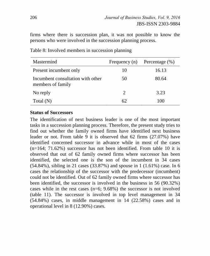
206 Journal of Business Studies, Vol. 9, 2016
JBS-ISSN 2303-9884
firms where there is succession plan, it was not possible to know the
persons who were involved in the succession planning process.
Table 8: Involved members in succession planning
Mastermind Frequency (n) Percentage (%)
Present incumbent only 10 16.13
Incumbent consultation with other
members of family
50 80.64
No reply 2 3.23
Total (N) 62 100
Status of Successors
The identification of next business leader is one of the most important
tasks in a succession planning process. Therefore, the present study tries to
find out whether the family owned firms have identified next business
leader or not. From table 9 it is observed that 62 firms (27.07%) have
identified concerned successor in advance while in most of the cases
(n=164; 71.62%) successor has not been identified. From table 10 it is
observed that out of 62 family owned firms where successor has been
identified, the selected one is the son of the incumbent in 34 cases
(54.84%), sibling in 21 cases (33.87%) and spouse in 1 (1.61%) case. In 6
cases the relationship of the successor with the predecessor (incumbent)
could not be identified. Out of 62 family owned firms where successor has
been identified, the successor is involved in the business in 56 (90.32%)
cases while in the rest cases (n=6; 9.68%) the successor is not involved
(table 11). The successor is involved in top level management in 34
(54.84%) cases, in middle management in 14 (22.58%) cases and in
operational level in 8 (12.90%) cases.
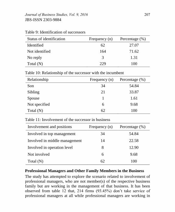
Journal of Business Studies, Vol. 9, 2016 207
JBS-ISSN 2303-9884
Table 9: Identification of successors
Status of identification Frequency (n) Percentage (%)
Identified 62 27.07
Not identified 164 71.62
No reply 3 1.31
Total (N) 229 100
Table 10: Relationship of the successor with the incumbent
Relationship Frequency (n) Percentage (%)
Son 34 54.84
Sibling 21 33.87
Spouse 1 1.61
Not specified 6 9.68
Total (N) 62 100
Table 11: Involvement of the successor in business
Involvement and positions Frequency (n) Percentage (%)
Involved in top management 34 54.84
Involved in middle management 14 22.58
Involved in operation level 8 12.90
Not involved 6 9.68
Total (N) 62 100
Professional Managers and Other Family Members in the Business
The study has attempted to explore the scenario related to involvement of
professional managers, who are not member(s) of the respective business
family but are working in the management of that business. It has been
observed from table 12 that, 214 firms (93.45%) don‟t take service of
professional managers at all while professional managers are working in
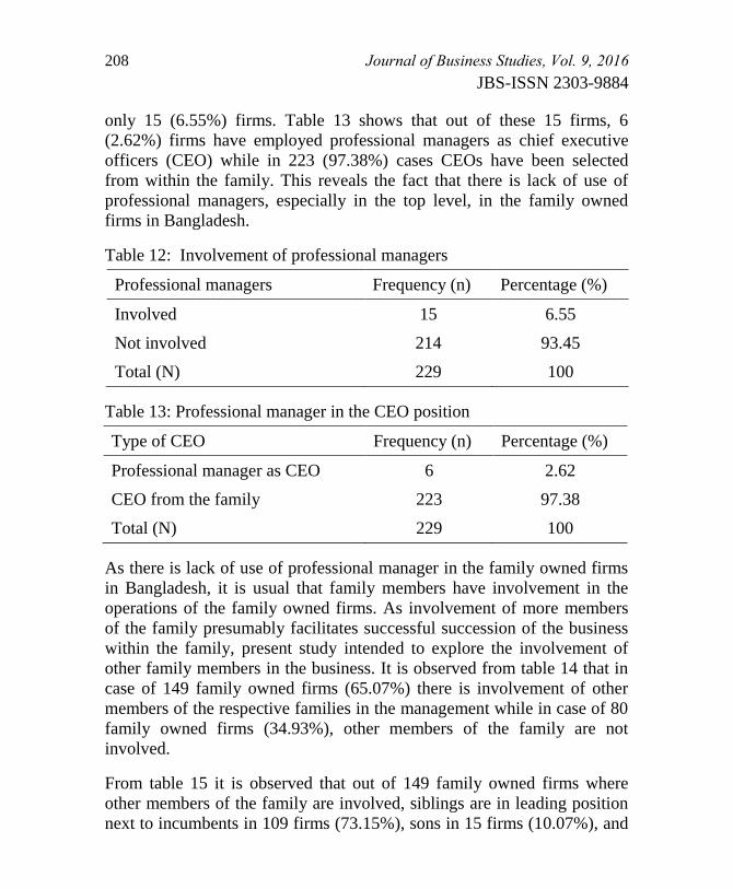
208 Journal of Business Studies, Vol. 9, 2016
JBS-ISSN 2303-9884
only 15 (6.55%) firms. Table 13 shows that out of these 15 firms, 6
(2.62%) firms have employed professional managers as chief executive
officers (CEO) while in 223 (97.38%) cases CEOs have been selected
from within the family. This reveals the fact that there is lack of use of
professional managers, especially in the top level, in the family owned
firms in Bangladesh.
Table 12: Involvement of professional managers
Professional managers Frequency (n) Percentage (%)
Involved 15 6.55
Not involved 214 93.45
Total (N) 229 100
Table 13: Professional manager in the CEO position
Type of CEO Frequency (n) Percentage (%)
Professional manager as CEO 6 2.62
CEO from the family 223 97.38
Total (N) 229 100
As there is lack of use of professional manager in the family owned firms
in Bangladesh, it is usual that family members have involvement in the
operations of the family owned firms. As involvement of more members
of the family presumably facilitates successful succession of the business
within the family, present study intended to explore the involvement of
other family members in the business. It is observed from table 14 that in
case of 149 family owned firms (65.07%) there is involvement of other
members of the respective families in the management while in case of 80
family owned firms (34.93%), other members of the family are not
involved.
From table 15 it is observed that out of 149 family owned firms where
other members of the family are involved, siblings are in leading position
next to incumbents in 109 firms (73.15%), sons in 15 firms (10.07%), and
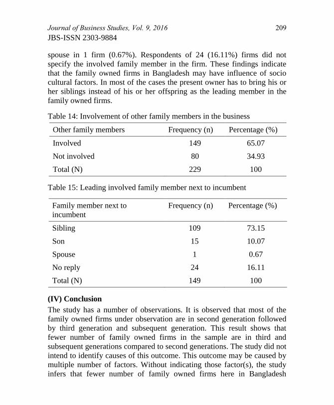
Journal of Business Studies, Vol. 9, 2016 209
JBS-ISSN 2303-9884
spouse in 1 firm (0.67%). Respondents of 24 (16.11%) firms did not
specify the involved family member in the firm. These findings indicate
that the family owned firms in Bangladesh may have influence of socio
cultural factors. In most of the cases the present owner has to bring his or
her siblings instead of his or her offspring as the leading member in the
family owned firms.
Table 14: Involvement of other family members in the business
Other family members Frequency (n) Percentage (%)
Involved 149 65.07
Not involved 80 34.93
Total (N) 229 100
Table 15: Leading involved family member next to incumbent
Family member next to
incumbent
Frequency (n) Percentage (%)
Sibling 109 73.15
Son 15 10.07
Spouse 1 0.67
No reply 24 16.11
Total (N) 149 100
(IV) Conclusion
The study has a number of observations. It is observed that most of the
family owned firms under observation are in second generation followed
by third generation and subsequent generation. This result shows that
fewer number of family owned firms in the sample are in third and
subsequent generations compared to second generations. The study did not
intend to identify causes of this outcome. This outcome may be caused by
multiple number of factors. Without indicating those factor(s), the study
infers that fewer number of family owned firms here in Bangladesh

210 Journal of Business Studies, Vol. 9, 2016
JBS-ISSN 2303-9884
survive in third and subsequent generations. The study finds lack of
existence of succession plan in the family owned firms in Bangladesh. In
most of the cases there is no succession plan. Out of the firms that have
succession plan, only a few of them have written succession plan while in
most of the firms succession plan is informal and not written. Therefore,
existence of formal written succession plan is pretty low in the family
owned firms in Bangladesh.
It is also observed that, there is high involvement of other family members
in the firms in Bangladesh where siblings of the incumbents are in leading
position next to him. Siblings are selected as successors in 33.87% of
those cases where successors have been identified. Therefore, though sons
of the incumbents are the leading selected successors, siblings are
important part in the succession of family owned firms in Bangladesh. It
has been observed from the study that a significant number of previous
owners are somehow active in the business. As involvement of the
previous owner in the business indicates incomplete succession, this
finding indicates that there are a large number of cases of incomplete
succession in family owned firms in Bangladesh.
As in Bangladesh very small number of studies has been conducted on
succession planning in family owned firms, the present study recommends
further in depth study on similar issues on family owned firms in
Bangladesh. The study hopes that findings of the study will provide
guidelines to the incumbents of family owned firms and academicians of
Bangladesh. The study also hopes that it will create a new trend of
research in business administration in Bangladesh and that will help in
long run survival of family owned firms and sustainable economic growth
of the country.

Journal of Business Studies, Vol. 9, 2016 211
JBS-ISSN 2303-9884
References
Aronoff, C. E. (1999). Family business survival: Understanding the
statistics “only 30%.” Family Business Advisor, 8(7), 1.
Chrisman, J. J., Chua, J. H., & Steier, L. (2005). sources and consequences
of distinctive familiness: an introduction. Entrepreneurship Theory
and Practice, May, 237-247.
Danco, L. (1982). Beyond survival a business owner’s guide for success.
Cleveland, OH: University Press.
Dyer, W. G., Jr. (1986). Cultural Change in Family Firms: Anticipating
and Managing Business and FamilyTransitions. San Francisco:
Jossey-Bass.
Gallo, M. A. (1995). Family businesses in Spain: Tracks followed and
outcomes reached by those among the largest thousand. Family
Business Review, 8(4), 245-254.
Handler, W. C. (1990). Succession in family firms: A mutual role
adjustment between entrepreneur and next-generation family
members. Entrepreneurship Theory and Practice, 15(1), 37–51.
Ibrahim, A. B., & Ellis, W. (1994). Family business management,
concepts and practice. Iowa: Kendall/Hunt.
Ibrahim, A. B., Soufani, K., & Lam., J. (2001). A Study of succession in a
Family Firm. Family Business Review, 16(3), 245-258.
Islam, M. S., Aleem, M. & Chowdhury, S. (2014). Role of predecessor in
successful succession in family owned firms, Journal of Business
Studies, 7 (January-June), 1-21.
Kepner, E. (1983). The family and the firm: A coevolutionary perspective.
Organizational Dynamics, 12, 57-70.
Kets de Vries, M.F.R. (1993). The dynamics of family controlled firms:
The good news and the bad news. Organizational Dynamics, 21,
59-71.

212 Journal of Business Studies, Vol. 9, 2016
JBS-ISSN 2303-9884
Lank, A. R., Owens, R., Martinez, J., Reidel, H., de Visscher, F., & Bruel,
M. (1994). The state of family business in various countries around
the world. The Family Business Network Newsletter, May, 3-7.
Lansberg, I. (1999). Succeeding generations: Realizing the dream of
families in business. Boston: Harvard Business School Press.
Le Breton-Miller, I., Miller, D., & Steier, L. P. (2004). Toward an
integrative model of effective FOB succession. Entrepreneurship
Theory and Practice, Summer, 305–328.
Miller, D., Steier, L., & Le Breton-Miller, I. (2003). Lost in time:
Intergenerational succession, change and failure in family
business. Journal of Business Venturing, 18(4), 513–551.
Nordqvist, M., (2005). Understanding the role of ownership in
strategizing - A study of family firms. Jönköping. JIBS Dissertation
Series No. 029.
NUTEK. (2004). B2004:06, Ägarskiften och ledarskiften i företag.
Stockholm: NUTEK förlag.
Poutziouris, P., O‟Sullivan, K., & Nicolescu, L. (1997). The [re]-
generation of family business entrepreneurship in the Balkans.
Family Business Review, 10(3), 239-260.
Poza, E. J. (1995). Global competition and the family- owned business in
Latin America. Family Business Review, 8(4), 301-311.
Ward, J. (1987). Keeping the family business healthy: How to plan for
continuing growth, profitability and family leadership. San
Francisco, CA: Jossey-Bass.
Ward, J. L. & Aronoff, C.E. (1992). Accountability: The Whetstone effect.
Nations Business, 80, 52-53.
Williams, R. (1992). Preparing your family to manage wealth. Marina,
CA: Monterey Pacific Institute.
Journal of Business Studies, Vol. 9, 2016 213
JBS-ISSN 2303-9884
Impact of Remittances to the Economic Development of
Bangladesh
Md. Omar Faruque 1
Udayshankar Sarkar 2
Abstract
examine the effect of workers’ remittance on Bangladesh economy.
To illustrate the effect of remittance, the paper uses the same national income
accounting framework as considered by Amjad R. (1986). Findings suggest that
the inflow of remittances increased from $0.2 billion in 1980 to $1.7 billion in
1999 that is about $1.5 billion increase over the 18 years. In the year of 1996-97,
remittances contributed almost 53.34% to overall balance of payment for
Bangladesh. Moreover, remittance contributed the highest of 62.12% in the year
1998. As remittances, GNP and remittance as percentage of GNP shows similar
trend in growth rate, this indicates that inflow of remittances positively
contributes to GNP. Furthermore, remittance earnings also positively contribute
to the Balance of Payments (BOP).
Keywords: Remittance, Balance of Payment, GDP, GNP
(I) Introduction
emittances to Bangladesh have been growing steadily over the last
decade. Since its independence in 1971, more than 3 million
Bangladeshis have left the country in search of employment. The central
bank estimates their cumulative remittances during 1976-2003 at round
US$22 billion (Amjad, 1989). Recognizing their economic importance,
the government for years has had legislation, policies, and an institutional
structure in place to facilitate the migration of its citizens. Now the
question is why sudden importance is put into the perception of
remittances? The fact is that the absolute and the relative volumes of
workers’ remittances are increasing. They have shown a steady increase
over the last decade. The amount of remittance flows to developing
countries already surpassed that of official resource inflows. Since 1999,
1 Assistant Professor, Department of Finance, Jagannath University,
Email: [email protected] 2 Department of Finance, Jagannath University,
Email: [email protected]
R
214 Journal of Business Studies, Vol. 9, 2016
JBS-ISSN 2303-9884
workers’ remittances have been the second largest resource flowing into
developing countries after foreign direct investment (FDI). In addition,
workers’ remittances are not liabilities but cash transfers from overseas,
which in principle, they do not cost any to recipient countries. As there has
been much debate about external debt and its negative effect on growth,
this feature is very attractive force. Despite the growing interest in
workers’ remittances, the role of remittance in development and economic
growth in general is not clearly understood. For example, studies based on
a country’s time-series data tend to find positive impacts of remittances on
growth, but a cross-country/panel data study by Hear and Sorensen (2003)
shows the opposite outcome. This is still one of the least studied areas of
research in migration literature. Despite the expanding literature on the
subject, there remains an inadequate understanding of a number of issues
related to the flow and use of remittances. Thus, there has been little work
on the impact of remittances on the overall economy.
The major labor exporting countries follow different conventions on
whether to include remittances from overseas workers as a part of the net
factor income in national income accounts. The resulting GNP estimates
(GNP= GDP + net factor income from abroad) therefore are not
comparable. Amongst the major Asian labor exporting countries, GNP
estimates published by governments in India, Sri Lanka, and Thailand
exclude workers’ remittances while Bangladesh, Pakistan and Philippines
include them.
In this , an attempt has been made to clarify concepts relating to the
affect of workers’ remittances on the overall economy of Bangladesh. As
Bangladesh is among the few countries that include workers’ remittances
separately in their gross national income estimates, it is important to
identify the impact of remittance on the national economy. In order to
understand the effect, this paper integrates remittance in the national
income accounting framework.
(II) Statement of the Problem
I bal and Sorensen (2003) have conducted a research on the impact of
workers’ remittance from the Middle East on Pakistan’s economy. The
research is based on the concept that inflow of remittance can have a
profound effect on Pakistan economy. The study reveals that significant
Journal of Business Studies, Vol. 9, 2016 215
JBS-ISSN 2303-9884
inflow of remittance will add to the society’s resources; ease the balance
of payment constraint, positively contribute to the Gross National Product
(GNP) and help gross national savings to increase. There is another study
conducted by Bruyn & Kuddus (2005) on ―Dynamics of Remittance
Utilization in Bangladesh‖. The study reveals that remittance has strong
impact on the national economy. In the current study use national
income accounting identity to analyze such effects of remittance on
Bangladesh economy. In this current research, to analyze the
effect of remittance on Bangladesh economy.
(III) Review of Literature
Remittance
When migrants send home part of their earnings in the form of either cash
or goods to support their families, these transfers are known as workers’ or
migrant remittances. Remittances have been growing rapidly in the past
few years and now represent the largest source of foreign income for many
developing countries. The official data on the inflow of remittances into
Bangladesh refers to the transfer of funds made by migrant workers
through the banking channel (and through post offices) (Mahmud, 1989).
The records of such transfers can be easily separated from other foreign
exchange transactions since these take place under what is known as the
Wage Earners’ Scheme (WES).
According to Ratha (2005), it is hard to estimate the exact size of
remittance flows because many transfers take place through unofficial
channels. Worldwide, officially recorded international migrant remittances
are projected to exceed $232 billion in 2005, with $167 billion flowing to
developing countries. These flows are recorded in the balance of
payments; an international technical group is reviewing exactly how to
record them. Unrecorded flows through informal channels are believed to
be at least 50 percent larger than recorded flows. Not only are remittances
large but they are also more evenly distributed among developing
countries than capital flows, including foreign direct investment, most of
which goes to a few big emerging markets. In fact, remittances are
especially important for low-income countries. Remittances are typically
transfers from a well-meaning individual or family member to another
216 Journal of Business Studies, Vol. 9, 2016
JBS-ISSN 2303-9884
individual or household. They are targeted to meet specific needs of the
recipients and thus, tend to reduce poverty. In fact, World Bank studies,
based on household surveys conducted in the 1990s, suggest that
international remittance receipts helped lower poverty (measured by the
proportion of the population below the poverty line) by nearly 11
percentage points in Uganda, 6 percentage points in Bangladesh, and 5
percentage points in Ghana. In poorer households, remittance may finance
the purchase of basic consumption goods, housing, and children's
education and health care. In richer households, they may provide capital
for small businesses and entrepreneurial activities. They also help pay for
imports and external debt service, and in some countries, banks have been
able to rise overseas financing using future remittances as collateral.
Remittance flows tend to be more stable than capital flows, and they also
tend to be counter-cyclical—increasing during economic downturns or
after a natural disaster in the migrants' home countries, when private
capital flows tend to decrease. In countries affected by political conflict,
they often provide an economic lifeline to the poor. The World Bank
estimates that in Haiti they represented about 17 percent of GDP in 2005,
while in some areas of Somalia, they accounted for up to 40 percent of
GDP in the late 1990s. There are a number of potential costs associated
with remittances. Countries receiving migrants' remittances incur costs if
the emigrating workers are highly skilled, or if their departure creates
labor shortages. In addition, if remittances are large, the recipient country
could face an appreciation of the real exchange rate that may make its
economy less competitive internationally. Some argue that remittances can
also create dependency, undercutting recipients' incentives to work, and
thus slowing economic growth. But others argue that the negative
relationship between remittances and growth observed in some empirical
studies may simply reflect the counter-cyclical nature of remittances—that
is, the influence of growth on remittances rather than vice-versa.
Remittances may also have human costs. Migrants sometimes make
significant sacrifices—often including separation from family—and incur
risks to find work in another country. And they may have to work
extremely hard to save enough to send remittances.
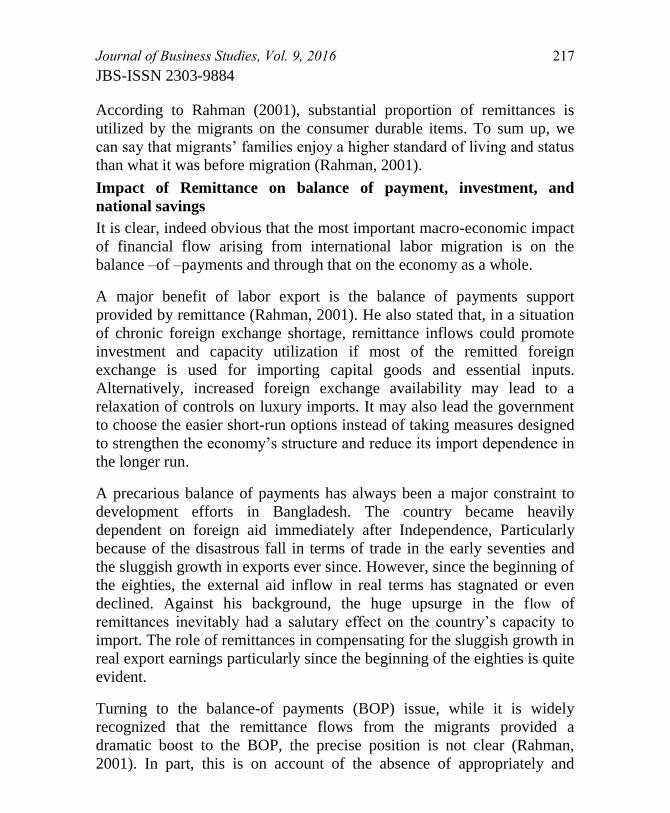
Journal of Business Studies, Vol. 9, 2016 217
JBS-ISSN 2303-9884
According to Rahman (2001), substantial proportion of remittances is
utilized by the migrants on the consumer durable items. To sum up, we
can say that migrants’ families enjoy a higher standard of living and status
than what it was before migration (Rahman, 2001).
Impact of Remittance on balance of payment, investment, and
national savings
It is clear, indeed obvious that the most important macro-economic impact
of financial flow arising from international labor migration is on the
balance –of –payments and through that on the economy as a whole.
A major benefit of labor export is the balance of payments support
provided by remittance (Rahman, 2001). He also stated that, in a situation
of chronic foreign exchange shortage, remittance inflows could promote
investment and capacity utilization if most of the remitted foreign
exchange is used for importing capital goods and essential inputs.
Alternatively, increased foreign exchange availability may lead to a
relaxation of controls on luxury imports. It may also lead the government
to choose the easier short-run options instead of taking measures designed
to strengthen the economy’s structure and reduce its import dependence in
the longer run.
A precarious balance of payments has always been a major constraint to
development efforts in Bangladesh. The country became heavily
dependent on foreign aid immediately after Independence, Particularly
because of the disastrous fall in terms of trade in the early seventies and
the sluggish growth in exports ever since. However, since the beginning of
the eighties, the external aid inflow in real terms has stagnated or even
declined. Against his background, the huge upsurge in the f of
remittances inevitably had a salutary effect on the country’s capacity to
import. The role of remittances in compensating for the sluggish growth in
real export earnings particularly since the beginning of the eighties is quite
evident.
Turning to the balance-of payments (BOP) issue, while it is widely
recognized that the remittance flows from the migrants provided a
dramatic boost to the BOP, the precise position is not clear (Rahman,
2001). In part, this is on account of the absence of appropriately and
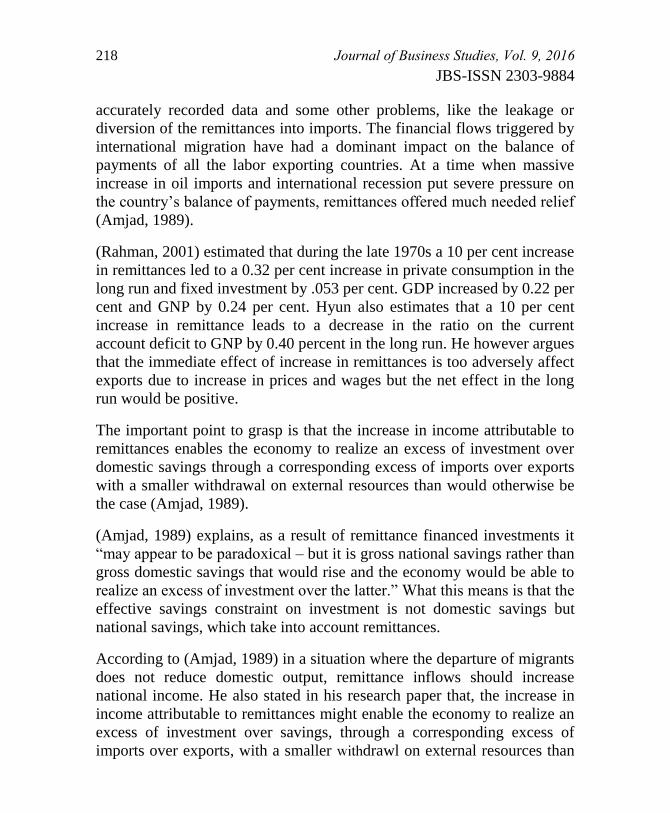
218 Journal of Business Studies, Vol. 9, 2016
JBS-ISSN 2303-9884
accurately recorded data and some other problems, like the leakage or
diversion of the remittances into imports. The financial flows triggered by
international migration have had a dominant impact on the balance of
payments of all the labor exporting countries. At a time when massive
increase in oil imports and international recession put severe pressure on
the country’s balance of payments, remittances offered much needed relief
(Amjad, 1989).
(Rahman, 2001) estimated that during the late 1970s a 10 per cent increase
in remittances led to a 0.32 per cent increase in private consumption in the
long run and fixed investment by .053 per cent. GDP increased by 0.22 per
cent and GNP by 0.24 per cent. Hyun also estimates that a 10 per cent
increase in remittance leads to a decrease in the ratio on the current
account deficit to GNP by 0.40 percent in the long run. He however argues
that the immediate effect of increase in remittances is too adversely affect
exports due to increase in prices and wages but the net effect in the long
run would be positive.
The important point to grasp is that the increase in income attributable to
remittances enables the economy to realize an excess of investment over
domestic savings through a corresponding excess of imports over exports
with a smaller withdrawal on external resources than would otherwise be
the case (Amjad, 1989).
(Amjad, 1989) explains, as a result of remittance financed investments it
―may appear to be paradoxical – but it is gross national savings rather than
gross domestic savings that would rise and the economy would be able to
realize an excess of investment over the latter.‖ What this means is that the
effective savings constraint on investment is not domestic savings but
national savings, which take into account remittances.
According to (Amjad, 1989) in a situation where the departure of migrants
does not reduce domestic output, remittance inflows should increase
national income. He also stated in his research paper that, the increase in
income attributable to remittances might enable the economy to realize an
excess of investment over savings, through a corresponding excess of
imports over exports, with a smaller drawl on external resources than

Journal of Business Studies, Vol. 9, 2016 219
JBS-ISSN 2303-9884
would otherwise be the case. Unless the marginal propensity to absorb out
foreign incomes exceeds unity, remittance inflows should always improve
the balance of payments position or prevent it from deteriorating as much
as it otherwise would.
The increased inflow of remittances significantly improved the balance of
payment position of Pakistan’s economy during the second half of the
seventies and early eighties. The foreign exchange made available because
of workers’ remittances also reduced the external debt, improved debt
servicing ability, and decreased the nee for additional foreign loans
(Nikos, 2005).
(IV) Methodology
Keynes National Income Accounting framework is used to determine the
effect of remittance on the economy of Bangladesh. This will provide an
important insight how workers remittances affect the economy. To
illustrate the effect of remittance, this paper uses the same national income
accounting framework that was used by Amjad R. (1986), in his paper
―Impact of Workers’ Remittances from Middle East on Pakistan
Economy: Some Selected Issues- the Pakistan Development Review
(1986)‖
To analyze the significance of migrant workers’ earning at the aggregate
level we will review data on imports, exports, workers’ remittances,
national and domestic savings, GNP, GDP, Net Income, Net Current
Transfers, Trade Balance, debt payment and investment. These data
accompanied with some other related data will be inserted in the MS Excel
software to run the analysis.
The Data
The data for the study is obtained from World Development Indicator (CD
ROM-2008-2009). Gross National Product (GNP), Gross Domestic
Product (GDP), Workers’ Remittance, Domestic and National Savings,
Capital Investment, Export and import of goods and services are collected
in current US$. The GDP Deflator (2005=100) is also obtained from the
WDI CD-ROM. All the variables are expressed in real terms by deflating
the data using GDP deflator (2005=100). The GNP figures are expressed
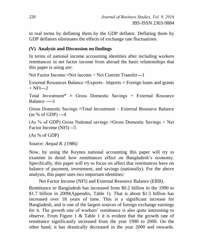
220 Journal of Business Studies, Vol. 9, 2016
JBS-ISSN 2303-9884
in real terms by deflating them by the GDP deflator. Deflating them by
GDP deflators eliminates the effects of exchange rate fluctuations.
(V) Analysis and Discussion on findings
In terms of national income accounting identities after including workers
remittances in net factor income from abroad the basic relationships that
this paper is using are:
Net Factor Income ≡Net income + Net Current Transfer---1
External Resources Balance ≡Exports– Imports + Foreign loans and grants
+ NFI---2
Total Investment* ≡ Gross Domestic Savings + External Resource
Balance ----3
Gross Domestic Savings ≡Total Investment – External Resource Balance
(as % of GDP) ---4
(As % of GDP) Gross National savings ≡Gross Domestic Savings + Net
Factor Income (NFI) --5
(As % of GDP)
Source: Amjad R. (1986)
Now, by using the Keynes national accounting this paper will try to
examine in detail how remittances effect on Bangladesh’s economy.
Specifically, this paper will try to focus on affect that remittances have on
balance of payment, investment, and savings (nationally). For the above
analysis, this paper uses two important identities:
Net Factor Income (NFI) and External Resource Balance (ERB).
Remittance to Bangladesh has increased from $0.2 billion in the 1990 to
$1.7 billion in 2009(Appendix, Table 1). That is about $1.5 billion has
increased over 18 years of time. This is a significant increase for
Bangladesh, and is one of the largest sources of foreign exchange earnings
for it. The growth rate of workers’ remittance is also quite interesting to
observe. From Figure 1 & Table 1 it is evident that the growth rate of
remittance significantly increased from the year 1990 to 2000. On the
other hand, it has drastically decreased in the year 2000 and onwards.
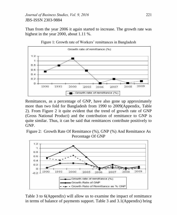
Journal of Business Studies, Vol. 9, 2016 221
JBS-ISSN 2303-9884
Than from the year 2006 it again started to increase. The growth rate was
highest in the year 2000, about 1.11 %.
Figure 1: Growth rate of Workers’ remittances in Bangladesh
Remittances, as a percentage of GNP, have also gone up approximately
more than two fold for Bangladesh from 1990 to 2009(Appendix, Table
2). From Figure 2 it quite evident that the trend of growth rate of GNP
(Gross National Product) and the contribution of remittance to GNP is
quite similar. Thus, it can be said that remittances contribute positively to
GNP.
Figure 2: Growth Rate Of Remittance (%), GNP (%) And Remittance As
Percentage Of GNP
Table 3 to 6(Appendix) will allow us to examine the impact of remittance
in terms of balance of payments support. Table 3 and 3.1(Appendix) bring
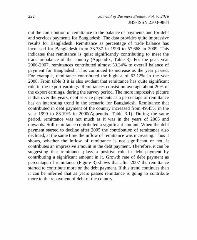
222 Journal of Business Studies, Vol. 9, 2016
JBS-ISSN 2303-9884
out the contribution of remittance to the balance of payments and for debt
and services payments for Bangladesh. The data provides quite impressive
results for Bangladesh. Remittance as percentage of trade balance has
increased for Bangladesh from 33.737 in 1990 to 57.668 in 2009. This
indicates that remittance is quiet significantly contributing to meet the
trade imbalance of the country (Appendix, Table 3). For the peak year
2006-2007, remittances contributed almost 53.34% to overall balance of
payment for Bangladesh. This continued to increase as the year passed.
For example, remittance contributed the highest of 62.12% in the year
2008. From table 3 it is also evident that remittance has quite significant
role in the export earnings. Remittances consist on average about 20% of
the export earnings, during the survey period. The more impressive picture
is that over the years, debt service payments as a percentage of remittance
has an interesting trend in the scenario for Bangladesh. Remittance that
contributed in debt payment of the country increased from 49.45% in the
year 1990 to 83.19% in 2000(Appendix, Table 3.1). During the same
period, remittance was not much as it was in the years of 2005 and
onwards. Still remittance contributed a significant amount. When the debt
payment started to decline after 2005 the contribution of remittance also
declined, at the same time the inflow of remittance was increasing. Thus it
shows, whether the inflow of remittance is not significant or not, it
contributes an impressive amount in the debt payment. Therefore, it can be
suggesting that remittance plays a positive role in debt payment by
contributing a significant amount in it. Growth rate of debt payment as
percentage of remittance (Figure 3) shows that after 2007 the remittance
started to contribute more on the debt payment. If this trend continues than
it can be inferred that as years passes remittance is going to contribute
more to the repayment of debt of the country.
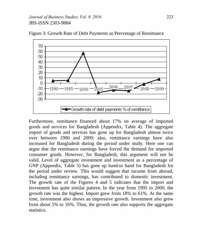
Journal of Business Studies, Vol. 9, 2016 223
JBS-ISSN 2303-9884
Figure 3: Growth Rate of Debt Payments as Percentage of Remittance
Furthermore, remittance financed about 17% on average of imported
goods and services for Bangladesh (Appendix, Table 4). The aggregate
import of goods and services has gone up for Bangladesh almost twice
over between 1990 and 2009; also, remittance earnings have also
increased for Bangladesh during the period under study. Here one can
argue that the remittance earnings have forced the demand for imported
consumer goods. However, for Bangladesh, this argument will not be
valid. Level of aggregate investment and investment as a percentage of
GNP (Appendix, Table 5) has gone up hand-to hand for Bangladesh for
the period under review. This would suggest that income from abroad,
including remittance earnings, has contributed to domestic investment.
The growth rate of the Figures 4 and 5 indicates that the import and
investment has quite similar pattern. In the year from 1995 to 2000, the
growth rate was the highest. Import grew from 18% to 61%. At the same
time, investment also shows an impressive growth. Investment also grew
from about 5% to 16%. Thus, the growth rate also supports the aggregate
statistics.
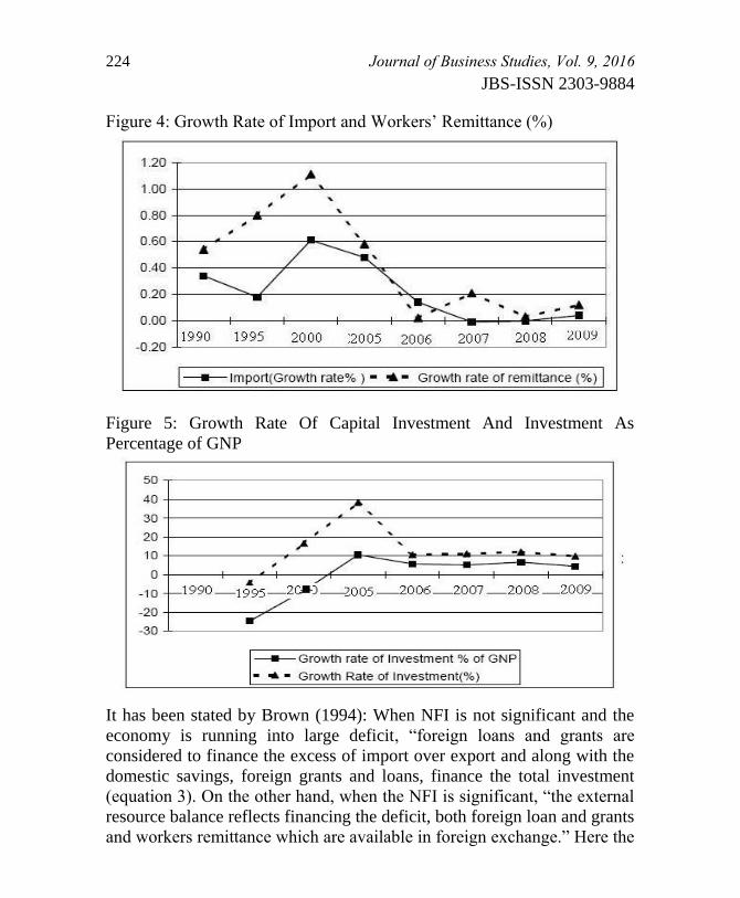
224 Journal of Business Studies, Vol. 9, 2016
JBS-ISSN 2303-9884
Figure 4: Growth Rate of Import and Workers’ Remittance (%)
Figure 5: Growth Rate Of Capital Investment And Investment As
Percentage of GNP
It has been stated by Brown (1994): When NFI is not significant and the
economy is running into large deficit, ―foreign loans and grants are
considered to finance the excess of import over export and along with the
domestic savings, foreign grants and loans, finance the total investment
(equation 3). On the other hand, when the NFI is significant, ―the external
resource balance reflects financing the deficit, both foreign loan and grants
and workers remittance which are available in foreign exchange.‖ Here the

Journal of Business Studies, Vol. 9, 2016 225
JBS-ISSN 2303-9884
foreign exchange, which is available to the domestic economy, will
enhance the national savings. According to Amjad.R (1986), the earlier
identity states that when the NFI (which includes the workers remittances)
is significant, reliance on sources like foreign loans and grants to finance
the investment decreases as national savings increases (as NFI increases;
NS=DS+ NFI) However, period under review for Bangladesh NFI (NFI,
equation 1) is significant (Appendix, Table 6 and Figure 6). Thus, it can be
said that the external resource balance (ERB, equation 2) Table
6(Appendix) and figure 6, in terms of financing the deficit, both foreign
loans and grants and workers remittance are used.
Figure 6: Time-Trend of Net Factor Income and External Resource
Balance
To know how much ERB is being financed by NFI, take the difference
between domestic and national savings (National savings= domestic
savings + NFI). Table 7 shows gross national savings has gone up for
Bangladesh; therefore, there is a positive contribution to ERB (i.e.
financed by workers’ remittance earnings). Therefore, as NFI is
significant, it helps to lessen the dependence on sources like foreign loans
and grants to finance the investment. About savings, Table 7(Appendix)
presents gross domestic savings, as a percentage of GDP, did not change

226 Journal of Business Studies, Vol. 9, 2016
JBS-ISSN 2303-9884
much between 2000 and 2009. Gross domestic savings is quite stable
compared to gross national savings. Gross national savings has increased
substantially during the survey period for Bangladesh. This reads as
increase in workers, remittances (plus other variables of NFI) substantially
decreased the dependence on foreign borrowings to finance investment.
The stable pattern of domestic savings for the economy illustrates that a
proportion of domestic consumption is being boosted due to increase in
foreign remittance earnings. For example, in the peak year of 2006 to 2007
remittance increased from 1.22 (billion US$) to 1.48 (billion US $) and at
the same time total consumption also increased from 32.92(billion US $)
to 34.36 (billion US $), which is quiet significant. On the other hand,
domestic savings only increased 1.17(billion US $) between those periods.
Figure 7: Trend of NFI, Gross Domestic Savings and Gross National
Savings
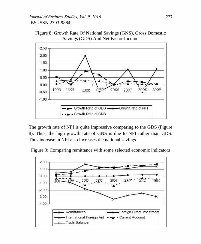
Journal of Business Studies, Vol. 9, 2016 227
JBS-ISSN 2303-9884
Figure 8: Growth Rate Of National Savings (GNS), Gross Domestic
Savings (GDS) And Net Factor Income
The growth rate of NFI is quite impressive comparing to the GDS (Figure
8). Thus, the high growth rate of GNS is due to NFI rather than GDS.
Thus increase in NFI also increases the national savings.
Figure 9: Comparing remittance with some selected economic indicators
228 Journal of Business Studies, Vol. 9, 2016
JBS-ISSN 2303-9884
Finally, when considering Table 8(Appendix) and Figure 9, remittances
significantly exceed foreign direct investment and foreign aid for
Bangladesh. From 2006 onwards, remittance earnings outweigh foreign
aid for Bangladesh. Incase of Bangladesh, remittance earnings partially
cover its trade deficit. One thing the reader should keep in mind that
remittance may finance consumer durable goods, but this will never
worsen the trade deficit. For example, if the remittance earning is $5,
import of goods cannot exceed $5, which is covered by the foreign
earnings the remittent sends. Now the only concern is if total remittance is
spent on consumption, it can lead to inflation in the economy but this
heavily depends on the elasticity of the goods, which are in high demand.
If inflow of remittances leads to increase in inflation, it might hurt others
welfare. (A micro level study is required to investigate this; a micro level
study can provide deeper insight into this problem. Considering viable
evidence from the countries under review, it is quite clear that remittance
earnings do not lead to inflation. As we already saw in our earlier
discussion, a fall in domestic savings is quite insignificant for Bangladesh
for the period under review). Consider the national income accounts, GNP
= GDP + NFI. From the above discussion, it has been found that NFI
(which includes workers’ remittance) is significant for Bangladesh in the
survey timeframe. Thus, it indicates that it also has quiet a significant
effect on the GNP.
(VI) Conclusion
Remittances to Bangladesh have been growing steadily over the past
decade. The study shows that the inflow of remittance in Bangladesh has
worked as a catalyst to restore the balance of payments deficits. The
inflow of remittances uniformly proved to be invaluable for Bangladesh,
by reducing the burden of debt payment, providing scarce foreign
exchange and finally boosting the national savings. From the analysis, the
economic benefits of inflow of remittance are clear. The finding of this
study, where remittance was integrated in the national income accounting
framework, brings out the importance of inflow of remittance in the
economy. The positive impact of remittances in economy would be much
clear, if further empirical study, using an econometric model is run.
Journal of Business Studies, Vol. 9, 2016 229
JBS-ISSN 2303-9884
References
Amjad, R. (Ed.). (1989). To the gulf and back. India: ILO. Asian
Development Bank, (2005). Quarterly Economic Update.
Bangladesh Resident Mission.
De Bruyn, T. & Kuddus, U. (2005), Dynamics of Remittance Utilization
in Bangladesh, IOM, Geneva.
De Bruyn, T. & Wets, J. (2004), ―Summary. Remittances as a
Development Tool. What Governments of Remittance Sending
Countries Can Do‖, paper presented at Novib International Expert
Meeting, Bridging the Gap: The Role of Migrants and Their
Remittances in Development, 19-20 November, Noordwijk,
Netherland.
De, Prabal, and Dilip Ratha. (2005). ―Remittance Income and Household
Welfare: Evidence from Sri Lanka Integrated Household Survey.‖
Economic Advisor’s Wing Finance Division, Ministry of Finance, (2004).
Bangladesh Economic Review. Ministry of Finance and Planning.
Economic Advisor’s Wing Finance Division, Ministry of Finance, (2005).
Bangladesh Economic Review. Ministry of Finance and Planning.
Fischer, S. & Startz, R. (1998). The Macroeconomics. New York: Gray
Burke.
Glytsos, P. Nicholas (2005). The contribution of remittances to growth. A
dynamic approach and empirical analysis, 32(6), 468-469.
GEP report (2008) ―Remittance helps poverty reduction‖ The
Independent. Published: November 24, 2005.
Hear, V. N. & Sorensen, N. N. (Eds.). (2003). The Migration-
Development Nexus. Switzerland: International Organization for
Migration.
Iqbal, K. & Ahmed, M. (Eds.). (2002). A study of remittance inflows and
utilization. Bangladesh: International Organization for Migration.
M. Mahmud (2006) ―Remittance grows 23pc in nine months‖ Vol. 5 Num
660, The Daily Star, link: http://archive.thedailystar.net
/2006/04/06 /d60406050154. htm.
230 Journal of Business Studies, Vol. 9, 2016
JBS-ISSN 2303-9884
Nikos, N. & Aggarwal, R. (Eds.). (2005). Migration Labour Remittances
in South Asia. Washington: The World Bank.
Osmani, S. R, & Mahmud, W. (2003). The Micro econimics of Proverty
Reduction: The case study of Bangladesh. Nepal: The Asia Pacific
of Regional Programme on Macroeconomics of Poverty
Reduction.
Rahman, A. (2001). Indian Labour Migration to the Gulf. New Delhi: Mrs.
Seema Wasan.
Raihan, A, & Mahmood, M. (Eds.). (2004). Trade Negotiations on
Temporary Movement of Natural Person: A Strategy Paper for
Bangladesh. Bangladesh: Center for Policy Dialogue.
Star Business Report (2008) ―Remittance grows 26pc in five months‖ The
Daily Star. Link: http://www.thedailystar.net/news-detail-26254
Report (2006) ―Remittance mark 23.75pc in 8 months‖ The Financial
Express. Published:08 March 2006.
Report (2006) ―Remittance closes to $3b in July-Feb" The New Age.
Published:08 March 2006.
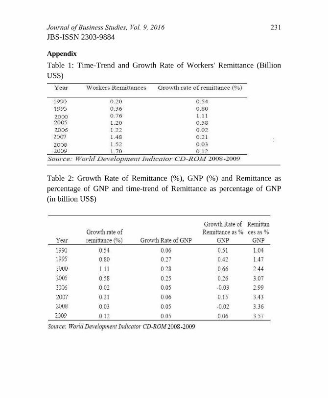
Journal of Business Studies, Vol. 9, 2016 231
JBS-ISSN 2303-9884
Appendix
Table 1: Time-Trend and Growth Rate of Workers' Remittance (Billion
US$)
Table 2: Growth Rate of Remittance (%), GNP (%) and Remittance as
percentage of GNP and time-trend of Remittance as percentage of GNP
(in billion US$)
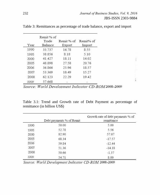
232 Journal of Business Studies, Vol. 9, 2016
JBS-ISSN 2303-9884
Table 3: Remittances as percentage of trade balance, export and import
Table 3.1: Trend and Growth rate of Debt Payment as percentage of
remittance (in billion US$)
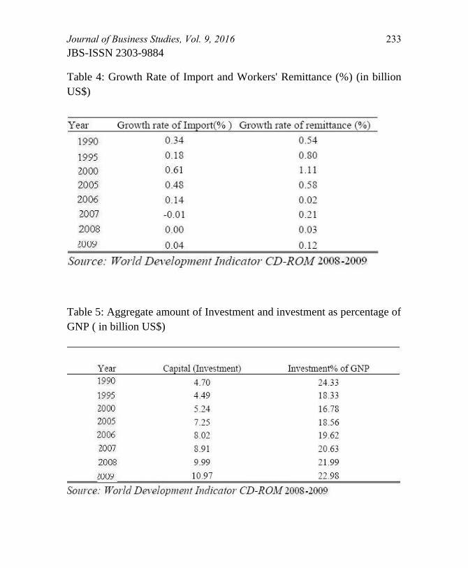
Journal of Business Studies, Vol. 9, 2016 233
JBS-ISSN 2303-9884
Table 4: Growth Rate of Import and Workers' Remittance (%) (in billion
US$)
Table 5: Aggregate amount of Investment and investment as percentage of
GNP ( in billion US$)
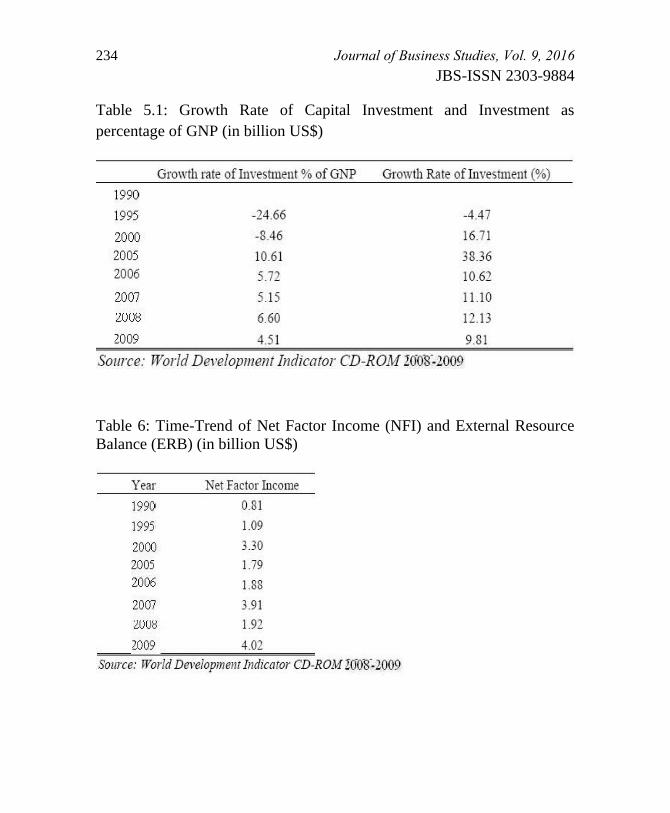
234 Journal of Business Studies, Vol. 9, 2016
JBS-ISSN 2303-9884
Table 5.1: Growth Rate of Capital Investment and Investment as
percentage of GNP (in billion US$)
Table 6: Time-Trend of Net Factor Income (NFI) and External Resource
Balance (ERB) (in billion US$)
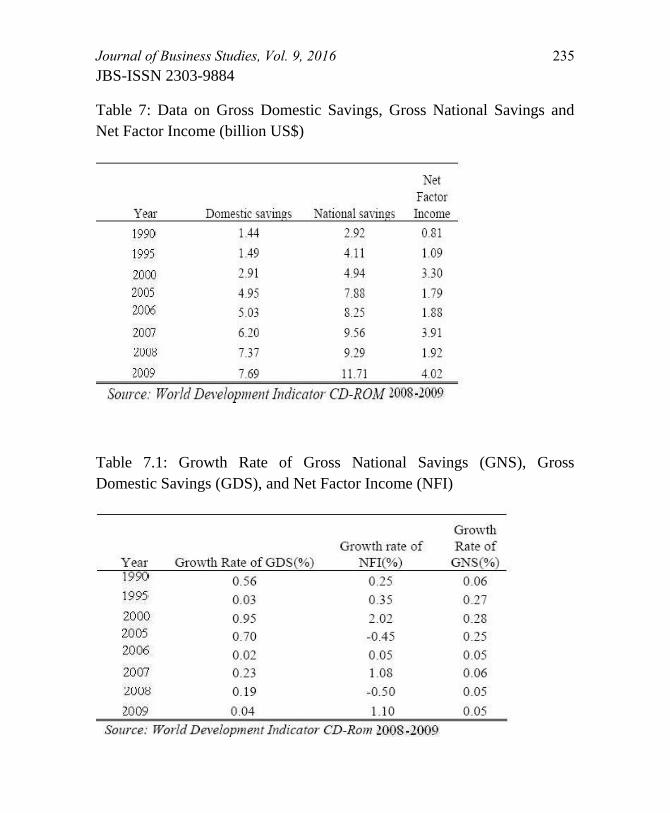
Journal of Business Studies, Vol. 9, 2016 235
JBS-ISSN 2303-9884
Table 7: Data on Gross Domestic Savings, Gross National Savings and
Net Factor Income (billion US$)
Table 7.1: Growth Rate of Gross National Savings (GNS), Gross
Domestic Savings (GDS), and Net Factor Income (NFI)
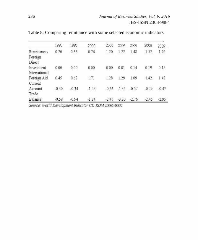
236 Journal of Business Studies, Vol. 9, 2016
JBS-ISSN 2303-9884
Table 8: Comparing remittance with some selected economic indicators

Contributors
Md. Ataul Gani OsmaniMd. Elias HossainAgricultural Commercialization in Bangladesh: Are Smallholder Farmers Market Oriented?
Dr. A S M KamruzzamanFactors affecting the choices for off-farm activities in Bangladesh: A study in Rajshahi District
Mahmud Hossain RiaziThe Economics of Price Volatility in Commodity Futures Markets: A Survey
Rakibul IslamImpact of Market Size and Foreign Trading on FDI Inflow in Bangladesh: A VEC Approach
Md. Abdul AlimRudrendu RayDr. Md Enayet HossainVisitors’ Perception towards Tour Destinations: A Study on Padma Garden
Ajit Kumar GhoseMd. Solaiman ChowdhuryDeterminants of Share Prices in Bangladesh: Evidence from Pharmaceuticals industry
Md. Ikbal HossainRebeka Sultana RekhaDr. Md. Enayet HossainInfluence of Cognitive and Affective Image on a Recreational Park: An Empirical Study
Mohammad Zahid Hossain, Ph.DMd. Fazle Fattah HossainPerformance Evaluation of Selected NCBs and PCBs in Bangladesh: An Empirical Study
Md. Shariful IslamProfessor Dr. Md. Amzad HossainSuccession Plan in Second or Subsequent Generation Family Owned Firms in Bangladesh- a Study in Rajshahi Division.
Md. Omar FaruqueUdayshankar SarkarImpact of Remittances to the Economic Development of Bangladesh