Journal of Computational Physics - brown.edu · Received in revised form 30 ... Journal of Computational Physics 228 (2009) ... IBM in that the force distribution effectively imposes

Journal of Computational Physics 228 (2009) 1750–1769

Contents lists available at ScienceDirect

Journal of Computational Physics

journal homepage: www.elsevier .com/locate / jcp

Smoothed profile method for particulate flows: Error analysisand simulations

Xian Luo, Martin R. Maxey, George Em Karniadakis *

Division of Applied Mathematics, Brown University, Providence, RI 02912, USA

a r t i c l e i n f o

Article history:Received 11 March 2008Received in revised form 30 September2008Accepted 5 November 2008Available online 20 November 2008

Keywords:SPMTwo-phase flowSuspensionsTime-splitting scheme

0021-9991/$ - see front matter � 2008 Elsevier Incdoi:10.1016/j.jcp.2008.11.006

* Corresponding author. Tel.: +1 401 863 1217; faE-mail addresses: [email protected], [email protected]

a b s t r a c t

We re-formulate and analyze a new method for particulate flows, the so-called ‘‘smoothedprofile” method (SPM) first proposed in [Y. Nakayama, R. Yamamoto, Simulation method toresolve hydrodynamic interactions in colloidal dispersions, Phys. Rev. E 71 (2005) 036707],which uses a fixed computational mesh without conformation to the geometry of the par-ticles. The method represents the particles by certain smoothed profiles to construct a bodyforce term added into the Navier–Stokes equations. SPM imposes accurately and efficientlythe proper conditions at the particle–fluid interface. In particular, while the originalmethod employs a fully-explicit time-integration scheme we develop a high-order semi-implicit splitting scheme, which we implement in the context of spectral/hp elementdiscretization. First, we show that the modeling error of SPM has a non-monotonic depen-dence on the time step size Dt; it is a function of

ffiffiffiffiffiffiffiffimDtp

=n, where m is the kinematic viscosityof fluid and n is the interface thickness of the smoothed profile. Subsequently, we pres-ent several steady and unsteady simulations, including flow past 3D complex-shaped par-ticles, and compare against direct numerical simulations and the force coupling method(FCM).

� 2008 Elsevier Inc. All rights reserved.

1. Introduction

Particulate flow occurs in many natural and technological situations, such as colloidal sedimentation, polymer suspen-sions and lubricated transport. The methods for numerical simulation of particulate flows can be broadly divided intotwo categories: the first one involves a Lagrangian description in which the computational mesh follows the particles orthe fluid; the second one employs an Eulerian description on a fixed grid with the interactions between the solvent andthe particles represented by some form of body force or appropriate interaction equations. For example, the arbitraryLagrangian–Eulerian (ALE) method [2,3] belongs to the first category, while the distributed Lagrange multiplier (DLM) meth-od first proposed by Glowinski et al. [4,5] and further developed by Patankar et al. [6] falls into the second category.

We have studied extensively in the past the force coupling method (FCM) [7–10], which is also a method in the secondcategory. It represents each particle in the flow by a low-order expansion of force multipoles, which is applied as a distrib-uted body force on the flow. It captures the far-field solution accurately and can typically resolve body forces with betterthan a couple of percent accuracy, though it does not fully resolve the flow field close to the particle surfaces (in the point-wise sense).

One of the most widely used methods in the second category is the immersed boundary method (IBM) of Peskin, whichwas originally developed for flows with immersed flexible membranes [11,12]. The main idea of IBM is to employ a regularEulerian mesh for the solvent over the entire domain, together with Lagrangian markers for the immersed boundary. The

. All rights reserved.

x: +1 401 863 3369.rown.edu (G.E. Karniadakis).

mailto:[email protected]

mailto:[email protected]

http://www.sciencedirect.com/science/journal/00219991

http://www.elsevier.com/locate/jcp

X. Luo et al. / Journal of Computational Physics 228 (2009) 1750–1769 1751

immersed boundary moves with the local fluid velocity, and in return exerts a ‘‘singular” force to the nearby fluid. This forceis usually obtained from the elastic properties of the immersed boundary, and then distributed into the surrounding fluidusing a regularized Dirac delta function. IBM was later extended to flows with rigid bodies with certain treatment, e.g. in[13,14]. A new ‘‘formally” second-order scheme of IBM was proposed in [15], which has less numerical viscosity and mightbe more appropriate for high Reynolds number flows. In these references [13–15], the fluid–particle interaction force utilizesa feed-back formulation, namely the ‘‘virtual boundary method” proposed in [16]. An alternative expression for the forcecalled ‘‘direct forcing” has been introduced to IBM by [17], which avoids introducing additional free parameters and allevi-ates the severe time step restrictions of the virtual boundary method. More recently, [18] proposed an improved direct forc-ing formulation which shows a smoother and less oscillatory boundary force for moving boundary problems. A similarapproach to IBM called ‘‘immersed interface method” (IIM) has been proposed in [19], and it was applied to Stokes flowproblems in [20]. In contrast to IBM adding the forcing function into the continuous governing equations, IIM incorporatesthe jump conditions across the immersed interfaces directly into the discrete equations. The IIM has been shown to be sec-ond-order accurate in the maximum norm for elliptic problems. Extension to incompressible Navier–Stokes equations hasbeen presented in [21,22]. The entire vector or only the normal component of the singular force (from the immersed inter-face to the fluid) is incorporated into jump conditions for both velocity and pressure or only pressure, in [21] and [22],respectively. They both give sharp resolution of the pressure across the interface. Compared to [22], the method in [21]achieves better accuracy, but it is more complicated to implement in general.

More recently, a new method, the so-called ‘‘smoothed profile” method (SPM), was proposed in [1,23–28]; it falls into thesecond category as well, for it uses a fixed grid. It is conceptually similar to FCM in the sense that it represents the particlesby certain smooth body forces in the Navier–Stokes equations instead of treating the particles as boundary conditions to thefluid. However, it has also features of IBM in that the force distribution effectively imposes constraints on the fluid motionthat approximate the boundary conditions. As with FCM and IBM, SPM solves a single set of fluid dynamics equations in theentire domain including the particle volumes, without any internal boundary conditions. However, different to FCM and IBM,a smoothly spreading interface layer is used to represent the particle boundaries to have a transition from the rigid-bodymotion to the fluid motion. This treatment is similar to the method of PHYSALIS [29,30], which assumes a boundary layerto exist next to the particle surface, where the Stokes approximation is valid; PHYSALIS uses a local analytic solution ofthe Stokes equations near the particle. Both PHYSALIS and SPM smear out the sharp solid–fluid interface and replace it bya smooth layer, which should be sufficiently resolved by the spatial discretization.

The key point of SPM is to update the velocity inside each particle through the integration of a ‘‘penalty” body force toensure the rigidity of the particles. It imposes the no-slip boundary condition implicitly without any special treatment onthe solid–fluid boundaries. This feature is, of course, appealing as it corrects the near-particle behavior of FCM in an efficientmanner.

SPM has been verified by several test problems, and has also been applied to the sedimentation of hundreds of 2D col-loidal disks in [1,24]. More recently, the method was extended to multi-component fluids, such as charged colloids in elec-trolyte solutions in [25,26,31] and the electrophoresis of dense dispersions in [27,32]. However, this method lacks anyrigorous theoretical foundation and it has only been presented as a fully-explicit scheme, hence limiting the size of time stepto very small values. It has also been used in conjunction with uniform grids and simple particle shapes. To this end, we haveworked on an error analysis of this method and, in particular, its semi-implicit extension that we propose in the currentwork. In addition, we critically evaluate SPM, for first time, against direct numerical simulations (DNS) and FCM solutionsfor a number of problems, including steady and unsteady particulate flows, simple- and complex-shaped particle evolutions.All the results we present in this paper are based on three-dimensional simulations.

The paper is organized as follows. In Section 2 we present the main steps of SPM in the context of high-order discretiza-tions. Specifically, a third-order stiffly-stable splitting scheme is employed for temporal discretization and spectral elementsfor spatial discretization. In Section 3 we quantify the accuracy of SPM for several prototype flows. In Section 4 a further ver-ification of the method is presented through comparisons with other methods for complex-shaped particles. Section 5 pre-sents a SPM simulation of two interacting spheres in low Reynolds number. We conclude in Section 6 with a brief summary.

2. Formulation

2.1. Smoothed representation of particles

SPM represents each particle by a smoothed profile (or in other words an indicator/concentration function), which equalsunity in the particle domain, zero in the fluid domain, and varies smoothly between one and zero in the solid–fluid interfacialdomain. In [1], several analytical forms of the smoothed profile for spherical particles are presented. Among them, the fol-lowing profile is mostly used:

/iðx; tÞ ¼12

tanhai � jx� Rij

ni

� �þ 1

� �; ð1aÞ

where index i refers to the ith sphere, and ai, Ri, ni are respectively the radius, the position vector, and the interface thicknessparameter for the ith sphere. The indicator function /i is a function of spatial coordinates x and time t.

1752 X. Luo et al. / Journal of Computational Physics 228 (2009) 1750–1769

Here we extend the above formula to a more general form, which is effective for any particle shape:

/iðx; tÞ ¼12

tanh�diðx; tÞ

ni

� �þ 1

� �; ð1bÞ

where diðx; tÞ is the signed distance to the ith particle surface with positive value outside the particle and negative value in-side the particle. The calculation of diðx; tÞ is rather straightforward if particles are in simple shapes (boxes, spheres, etc.). If,however, we deal with more complex shapes which are represented by many surface points coordinates, a closest-pointsearching procedure should be used to find diðx; tÞ and thus /iðx; tÞ.

For other cases where we know the analytical form of the particle surface functions, or where we can construct an inter-polating spline function based on the surface points, we propose to use a slightly different form of the indicator function dueto its convenience and efficiency:

/iðx; tÞ ¼12

tanhfiðx; tÞ

nisi

� �þ 1

� �; ð2Þ

where fiðx; tÞ is the surface function of the ith particle, which is zero on the surface, positive inside the particle, and negativeoutside; here si is a scaling factor. We implement this form in most of the numerical simulations of flows involving spherical,ellipsoidal and biconcave particles, which are presented in the next two sections.

A smoothly spreading concentration field is achieved by summing up the concentration functions of all the Np non-over-lapping particles:

/ðx; tÞ ¼XNp

i¼1

/iðx; tÞ: ð3Þ

Fig. 1 shows a schematic of the smoothed profiles for an example involving two particles. The entire domain D can be sub-divided into three domain types: Dpi is the particle domain of the ith particle, where / � 1:0; Df is the fluid domain, where/ � 0:0; and Ds is the interface domain, where 0:0 < / < 1:0.

Based on this concentration field, the particle velocity field, upðx; tÞ, is constructed from the rigid motions of the Np

particles:

/ðx; tÞupðx; tÞ ¼XNp

i¼1

ViðtÞ þXiðtÞ � x� RiðtÞ½ �f g/iðx; tÞ; ð4Þ

where Ri, Vi ¼ dRidt and Xi are spatial positions, translational velocity and angular velocity of the ith particle, respectively. We

can verify that the divergence of the particle velocity field is identically zero, i.e.,

r � up ¼XNp

i¼1

ViðtÞ þXiðtÞ � ½x� RiðtÞ�f g � r /i

/

� �¼ 0;

P
where we have used: rð/i
/Þ ¼ðr/iÞ/�/iðr/Þ

/2 ¼Npj¼1½ðr/iÞ/j�/iðr/jÞ�

/2 ¼ 0, by the assumption of non-overlapping envelopes of differ-ent particles, i.e., /iðr/jÞ ¼ 0 for 8i–j.

The total velocity field is then defined by a smooth combination of both the particle velocity field up and the fluid velocityfield uf :

uðx; tÞ ¼ /ðx; tÞupðx; tÞ þ ð1� /ðx; tÞÞuf ðx; tÞ: ð5Þ

We see that inside the particle domain ð/ ¼ 1Þ, we have u ¼ up, i.e., the total velocity equals the particle velocity. In the inter-facial domain ð0 < / < 1Þ the total velocity changes smoothly from the particle velocity up to the fluid velocity uf .

0.80.60.40.2

φ

Dp1

Dp2

D

Df

Ds

Fig. 1. An example of two particles: contours of the concentration field / and computational domain partitioning ðD ¼PNp

i¼1Dpi þ Df þ DsÞ.


SPM imposes indirectly the no-slip constraint on the particle boundaries. This imposition can be verified by taking thecurl of Eq. (5):

r� u ¼ r� ½uf þ /ðup � uf Þ� ¼ ðr/Þ � ðup � uf Þ þ /ðr � upÞ þ ð1� /Þðr � uf Þ:

As r/ is non-zero in the interfacial domain and is perpendicular to the particle surface, the no-slip constraint can be ex-pressed as ðr/Þ � ðup � uf Þ ¼ 0. So the imposition of the no-slip constraint comes from the assumption that the vorticityof the total flow field consists of the vorticities from both the fluid velocity and the particle velocity, i.e.,

r� u ¼ /ðr � upÞ þ ð1� /Þðr � uf Þ: ð6Þ

The validity of this equation will be checked later in a numerical simulation example.SPM also imposes the no-penetration constraint on particle surfaces. If we check the divergence of the total velocity, tak-

ing into account that the fluid solvent is incompressible and the particle velocity field is divergence-free (derived by assum-ing non-overlapping particle envelopes), we obtain:

r � u ¼ r � ½uf þ /ðup � uf Þ� ¼ ðr/Þ � ðup � uf Þ: ð7Þ

Since ðr/Þ � ðup � uf Þ ¼ 0 represents the no-penetration constraint on particle surfaces, imposing the incompressibility con-dition of the total velocity r � u ¼ 0 ensures the no-penetration surface condition, and vice versa.

SPM solves for the total velocity, u, in the entire domain D, including the particle domain, using the Navier–Stokes equa-tions with an extra force density term along with the incompressibility constraint:

ouotþ ðu � rÞu ¼ � 1

qrpþ mr2uþ gþ fs in D; ð8aÞ

r � u ¼ 0 in D; ð8bÞ

where q is the density of the fluid, p is the pressure field, m is the kinematic viscosity of the fluid, g is the gravity (and otherexternal forces on the fluid), and fs is the body force density term representing the interactions between the particles and thefluid. Here, the fluid solvent is assumed to be Newtonian with constant viscosity for simplicity.

The velocity and pressure fields are solved through the following two-step semi-discrete form proposed in [1,25]. First,SPM solves for an intermediate velocity and pressure fields as u�; p� from the previous step solution un, by integrating theadvection and viscous stress:

u� ¼ un þZ tnþ1

tndt½�ðu � rÞu� 1

qrp� þ mr2uþ g�; ð9aÞ

� un þ Dt �ðun � rÞun � 1qrp� þ mr2un þ gn

� �in D; ð9bÞ

where Dt is the time increment tnþ1 � tn, and a forward Euler integration is used. This is solved in conjunction with theincompressibility constraint on u�, i.e., r � u� ¼ 0, and hence 1

qr2p� ¼ r � ½�ðun � rÞun þ gn�.

Then SPM updates the total velocity and pressure fields from u�;p�:

unþ1 ¼ u� þZ tnþ1

tndt fs �

1qrpp

� �¼ u� þ /ðup � u�Þ � Dt

qrpp

� �in D; ð10Þ

where pp is the extra pressure field and up is calculated from Eq. (4). Note that the particle motions (Vi and Xi) could either begiven or calculated from Newton’s equations using the exerted forces on the particle. SPM assigns

R tnþ1

tn fsdt ¼ /ðup � u�Þ todenote the momentum change (per unit mass) due to the presence of the particle. Thus at each time step the flow is cor-rected by a momentum impulse to ensure that the total velocity matches that of the rigid particles within the particle vol-ume, and hence to enforce the rigidity constraint. From the above expression we have that fs � 1

Dt /ðup � u�Þ, suggesting thatSPM is similar to penalty methods [33,34], which incorporate constraints into the governing equations. Here 1=Dt serves as apenalty parameter; thus the smaller Dt is, the tighter the control of the rigidity constraint is. However, in contrast to the deltafunctions used in [33,34], the smooth indicator function / is used here by SPM.

The total pressure field is split into two parts as: p ¼ p� þ pp to ensure the divergence-free of the total velocity fieldðr � u ¼ 0Þ and hence the imposition of the impermeable boundary condition on the particle boundaries. Specifically, the fol-lowing equation for pp:

Dtqr2pp ¼ r � ½/ðup � u�Þ� in D; ð11Þ

is derived by taking the divergence of Eq. (10) and using the divergence-free constraints r � u� ¼ 0, r � un ¼ 0 andr � unþ1 ¼ 0.


2.2. Semi-discrete system: temporal integration

The original SPM [1,25] used a fully-explicit time marching scheme for Eq. (9a). In the current paper, we introduce a semi-implicit treatment, using a stiffly-stable high-order splitting (velocity-correction) scheme [35], in order to enhance stabilityand increase temporal accuracy.

In the velocity-correction splitting scheme, the fields at time level n: fun, pn, Rni , On

i , /n, Vni , Xn

i , 8i ¼ 1; . . . ;Npg, are ad-vanced over a time step Dt to determine the fields funþ1; pnþ1, Rnþ1

i , Onþ1i , /nþ1, Vnþ1

i , Xnþ1i ,8i ¼ 1; . . . ;Npg, through the four

substeps outlined below. Note that Rni ;O

ni are position vector and orientation vector of the ith particle respectively, which

contribute to the concentration function /n.As a preliminary step before all substeps, we move particles from Rn

i ;Oni to Rnþ1

i ;Onþ1i by Vn

i ;Xni using an explicit integra-

tion scheme, e.g. a high-order Adam–Bashforth method as

Rnþ1i ¼ Rn

i þ DtXJe

q¼0

aqVn�qi ; ð12aÞ

Onþ1i ¼ On

i þ DtXJe

q¼0

aqXn�qi ; ð12bÞ

where Je is the order of the explicit time-integration scheme and aq are the coefficients in the Adam–Bashforth scheme. Then,the concentration field /nþ1 is calculated.

2.2.1. Velocity update due to advectionWe compute the intermediate velocity field us by first integrating the non-linear (advection) term and body force term:

us �PJe�1

q¼0 aqun�q

Dt¼XJe�1

q¼0

bq½�ððu � rÞuÞn�q þ gn�q� in D; ð13Þ

where aq; bq are the coefficients derived from the standard stiffly-stable scheme formulation (see [36]). Also, un�q and gn�q

are the velocity and body force fields at previous time steps.

2.2.2. Velocity update due to pressure influenceWe then update the velocity from us to uss to account for the pressure influence:

uss � us

Dt¼ �rp� in D; ð14Þ

where the intermediate pressure field p� is solved from:

r2p� ¼ r � us

Dt

� �in D: ð15Þ

This equation is derived from Eq. (14) by imposing the incompressibility constraintr � uss ¼ 0, following the velocity-correc-tion splitting scheme described in [36].

The following Neumann boundary condition for p� is used at any velocity Dirichlet boundary:

op�

on¼XJe�1

q¼0

bq½�ðu � rÞuþ g� mr� ðr� uÞ�n�q � n; ð16Þ

assuming time-independent normal velocities at the boundary (see [36]).

2.2.3. Viscous effectsWe obtain the intermediate velocity u� based on uss by treating the viscous term implicitly:

r2 � c0

mDt

� �u� ¼ � uss

mDtin D; ð17Þ

where c0 is the scaled coefficient of the stiffly-stable scheme with c0 ¼PJe�1

q¼0 aq. Here, the velocity u� on the boundary takesthe same values prescribed as boundary conditions.

2.2.4. Velocity update due to rigid-body motion constraintFirst, the hydrodynamic force and torque on the particles exerted by the surrounding fluid are derived from the momen-

tum conservation between the particles and the fluid. In other words, the momentum change in the particle and interfacialdomain equals the time integral of the hydrodynamic force and the external force. Hence, we assign


Fnhi¼ 1

Dt

ZDq/nþ1

i ðu� � unpÞdx�

ZD

/nþ1i qgdx; ð18aÞ

Nnhi¼ 1

Dt

ZD

rnþ1i � ½q/nþ1

i ðu� � unpÞ� �

ZD

/nþ1i rnþ1

i � ðqgÞdx; ð18bÞ

where rnþ1i is the distance vector from the rotational reference point on the ith particle to any spatial point x. Here, a first

order approximation is used in the force integration.Second, the particle translational and angular velocities are updated using Newton’s equations:

Vnþ1i ¼ Vn

i þM�1i � Dt �

XJe

q¼0

aq � ðFn�qhiþ Fn�q

extiÞ; ð19aÞ

Xnþ1i ¼ Xn

i þ I�1i � Dt �

XJe

q¼0

aq � ðNn�qhiþ Nn�q

extiÞ; ð19bÞ

where Mi and Ii are the mass and the moment of inertia of the ith particle, aq are the coefficients from a Adam–Bashforthscheme. Here, Fn�q

extiand Nn�q

extiare, respectively the external force and torque on the ith particle at previous time steps.

Third, the particle velocity field is calculated from:

/nþ1unþ1p ¼

XNp

i¼1

/nþ1i fVnþ1

i þXnþ1i � ½x� Rnþ1

i �g: ð20Þ

For free motion of particles, up is coupled with the forces and torques on particles Fhi; Fext i;Nhi and Next i. To decouple the sys-tem, we employ Eqs. (18),(19) and (20) using an explicit numerical scheme.

Fourth, we solve for the extra pressure field pp due to the rigidity of the particle as

r2pp ¼ c0r �/nþ1ðunþ1

p � u�ÞDt

!in D: ð21aÞ

The following is used as the boundary conditions for pp at any velocity Dirichlet boundary (with time-independent normalvelocities):

opp

on¼

c0/nþ1ðunþ1

p � u�ÞDt

� n: ð21bÞ

Finally, we update the total velocity field by enforcing the rigid-body motion constraint using the particle velocity field/nþ1unþ1

p :

c0unþ1 � c0u�

Dt¼

c0/nþ1ðunþ1

p � u�ÞDt

�rpp in D: ð22Þ

Eqs. (21a) and (21b) are both derived from Eq. (22). The total pressure field is calculated by summing the intermediate pres-sure and the extra pressure field, i.e., pnþ1 ¼ p� þ pp.

2.3. Fully-discrete system: spatial discretization

For spatial discretization of the above equations, we apply the spectral/hp element method (see [36]). This hybrid methodbenefits from both finite element and spectral discretization: on one hand, for domains with complex geometry, we can in-crease the number of subdomains/elements (h-refinement) with the error in the numerical solution decaying algebraically.On the other hand, with fixed elemental size we can increase the interpolation order within the elements (p-refinement) toachieve an exponentially decaying error, provided the solutions are sufficiently smooth throughout the domain. Hence, theuse of smoothed profiles in SPM preserves the high-order numerical accuracy of the spectral/hp element method.

The solution domain is partitioned into non-overlapping sub-domains/elements (with characteristic size of an element tobe h): X ¼

SNele¼1X

e. We use hexahedral or tetrahedral elements in our present numerical simulations. By constructing thestandard element Xst , the local coordinates in the standard element ðf 2 XstÞ can be mapped to the global coordinate inany elemental domain ðx 2 XeÞ by an isoparametric transformation x ¼ veðfÞ. Then, a polynomial expansion (with polyno-mial order up to P) is employed within the standard element to construct the approximate solution ud:

udðxÞ ¼XNel

e¼1

XP

j¼1

uej w

ej ðfÞ ¼

XNdof

i¼0

uiWiðxÞ; ð23Þ

where f ¼ ½ve��1ðxÞ is the local coordinate, wej ðfÞ denotes the local expansion modes, and WiðxÞ are the global modes derived

from the global assembly of the local modes [36].


For the expansion basis wej ðfÞ, both modal and nodal basis can be used. A modal expansion is used in conjunction with

Galerkin projection to solve Eqs. (15), (17) and (21a), while a nodal expansion is used in conjunction with collocation pro-jection of Eq. (13). The updating step (22) could be done by either collocation or Galerkin projection. The former is more effi-cient but the numerical solution might be discontinuous at some element boundaries, whereas the latter guarantees C0

continuity of the approximate solution across the elements through an appropriate choice of the boundary modes. Forthe modal expansion, we use a semi-orthogonal basis written in terms of the Jacobi polynomials. For the nodal basis, weemploy the Lagrange–Jacobi polynomials through the Gauss–Legendre–Lobatto quadrature points.

The spectral/hp element method allows us to accurately represent arbitrary fixed rigid boundaries of the flow domainwhile using SPM to represent the particles.

3. Prototype flows: error analysis and verification

In order to verify SPM and analyze its error, we test several prototype flow problems.

3.1. Planar Couette flow

We simulate the steady laminar flow of a viscous fluid between two parallel plates, one moving relatively to the other.The plates are separated by a distance h in the y-direction with the lower plate aligned with the x-axis and being stationarywhile the upper plate moving with constant velocity V ¼ ðV ;0;0Þ. At first, we want to see how accurately SPM captures theexact analytical solution uexact ¼ ðV � y=h;0;0Þ for y 2 ½0;h� and ðV ;0;0Þ for y 2 ½h;2h�; here we specify V ¼ 1;h ¼ 3.

Specifically, using this problem, we want to analyze SPM using two different time-discretization implementations: one isthe original fully-explicit scheme [1,25], while the other is the semi-implicit scheme we proposed in the previous section.The fully-explicit SPM uses two steps as in Eqs. (9a) and (10), while the semi-implicit SPM uses four steps given by Eqs.(13), (14), (17) and (22). The top wall ðh 6 y 6 2hÞ is treated by a ‘‘smoothed profile”, with the concentration field of/ðx; tÞ ¼ 1

2 tanh y�hn

� �þ 1

h iderived from Eq. (1b). The simulation domain D is a box of h=3� 2h� h=3, with periodic bound-

aries in the x- and z-directions and Dirichlet boundaries in the y-direction (i.e., ujy¼0 ¼ ð0;0;0Þ;ujy¼2h ¼ V ¼ ð1;0;0Þ). Weignore both the gravity and the advection ðu � rÞu in both implementations. The velocity and pressure fields are solvedby a first-order temporal scheme by marching through pseudo-time to the steady state. The spectral/hp element methodis used for spatial discretization, with six non-uniform elements and a polynomial order of P ¼ 11. Upon convergence tosteady state, we calculate the L2 error ðL2erÞ of the streamwise velocity u in the flow region 0 6 y 6 h.

We can also obtain solutions directly from the semi-discrete equations by assuming that: (1) all the field quantities areonly y-dependent, i.e., uðx; y; zÞ ¼ uðyÞ; pðx; y; zÞ ¼ pðyÞ, etc.; (2) the velocity field has a nontrivial component only in thestreamwise direction, i.e., uðyÞ ¼ ðuðyÞ;0;0Þ; (3) steady state is achieved, i.e., unþ1 ¼ un; and (4) the pressure is uniform every-where, i.e., rp� ¼ ð0;0;0Þ;rpp ¼ ð0;0;0Þ. Then for the fully-explicit implementation, from (9a) and (10), we obtain the 1Dreduced system for the streamwise velocity un and the streamwise intermediate velocity u�:

ð1� /ÞmDt o2un

oy2 � /un ¼ �/up;

u� ¼ un þ mDt o2un

oy2 :

8<: ð24Þ

Applying the same assumptions to the semi-implicit scheme, a different reduced system for un and u� is derived from Eqs. (13),(14), (17) and (22):

mDt o2u�oy2 � /u� ¼ �/up;

un ¼ u� þ /ðup � u�Þ:

(ð25Þ

From the above reduced systems, for both schemes we obtain the velocity to be: un ¼ up when / ¼ 1 (particle domain) andun ¼ u� ¼ ay when / ¼ 0 (fluid domain), where the constant a needs to be determined by matching the velocity through theinterface domain. In the limit of employing a step function for / (i.e., n ¼ 0), and by imposing C0 continuity of un at the inter-face y ¼ h, we find that a ¼ y=h, which means we recover the exact solution using both schemes. However, if / is a smoothfunction with n > 0, the above two reduced systems are solved by a second-order finite difference method using a fine uni-form grid (with 4001 grid points and mesh size Dy ¼ 2h=4000).

Furthermore, in both 1D systems (24) and (25), an artificial boundary layer (scaling asffiffiffiffiffiffiffiffimDtp

) is present. In particular, bothterms expðy=


Þwill be present in the velocity solution and this will lead to a non-monotonic error behavior. Our resultsfrom solving the full 3D system further verify this.

Fig. 2 shows that the L2 error in both implementations has a non-monotonic dependence on the time step Dt, similar infact to the error structure of semi-Lagrangian schemes [37]. We note that the spatial discretization error is negligible sinceincreasing the polynomial order in each element from P ¼ 11 to P ¼ 13 showed no change in the L2 error. The true temporaldiscretization error should also vanish for the high-order splitting scheme (see [36]). The agreement of the 4-step full 3Dsystem results with the 4-step reduced 1D system results in Fig. 2 indicates a negligible error of the pressure solver. Sothe L2 error shown in the figures consists of the SPM modeling error from the smoothed particle representation in the

Δt

L2er

0 0.005 0.01 0.0150

0.005

0.01

0.015

0.02 4-step RED, ξ0,ν04-step RED, 2ξ0,ν02-step RED, ξ0,ν02-step RED, 2ξ0,ν04-step FULL, ξ0,ν04-step FULL, 2ξ0,ν04-step FULL, ξ0,2ν0

Fig. 2. Couette flow: L2 error of the streamwise velocity versus Dt for two different interface thickness n and two different kinematic viscosity m. (LEGENDNOTE: ‘4-step’: 4-step semi-implicit scheme; ‘2-step’: 2-step full-explicit scheme; ‘RED’: reduced 1D system discretized by finite difference; ‘FULL’: full 3Dsystem discretized by spectral/hp element; ‘n0’: n0 ¼ 0:05 ¼ 0:0167h; ‘m0’: m0 ¼ 1:0.)


Navier–Stokes equation by Eqs. (9a) and (10). Simple scaling arguments of the 1D systems (24) and (25) show that the erroris, in fact, a function of


=n, and the results from the solution of the full 3D system shown in Fig. 3 verify this.Fig. 3 also indicates that the optimum time step size ðDtÞo depends only on

ffiffiffimp

=n, i.e., for the 2-step fully-explicit schemeffiffiffiffiffiffiffiffiffiffiffiffiffiffimðDtÞo

p=n � 0:88, while for the 4-step semi-implicit scheme

ffiffiffiffiffiffiffiffiffiffiffiffiffiffimðDtÞo

p=n � 0:75. A physical explanation of this error behavior

can be put forward by considering the following two aspects. On the one hand, recall that SPM essentially adds a penaltyterm fs � /ðup � u�Þ=Dt in the Navier–Stokes equations. Hence, smaller Dt would have a tighter control of the flow and thusachieve better accuracy. But on the other hand, physically SPM simulates the particle by impulsively applying a momentumchange to the particle domain at each time step, which in turn creates an impulse on the flow as in the Stokes’ first problem.The thickness of the diffusive layer (within which the impulsive momentum change has an effect) is thus scaled asd ¼ 2:76


[38]. So a smaller Dt will produce a thinner Stokes layer thickness d; in particular, if Dt is so small that d cannotbe spatially resolved by the smoothed profile used, it will lead to an increase in error. Let us introduce the ‘‘effective” smoothinterface thickness le, which is expected to be scaled as 2n. The optimum time step size ðDtÞo, which produces the smallesterror, comes from the balance of the Stokes layer scale d and the effective interface thickness le. The numerical results inFig. 3 verify this by showing that le ¼ 2:07n for the 4-step semi-implicit implementation. But for the 2-step fully-explicitscheme, a larger le ¼ 2:42n is indicated. By treating the viscous term implicitly in the 4-step scheme, we have a stricter con-trol of the viscous layer throughout the interface domain, thus the intermediate velocity u� is more sharply defined andhence the effective smooth interface thickness le is thinner.

L2er

(νΔt)0.5/ξ0.4 0.6 0.8 1 1.2 1.40

0.001

0.002

0.003

0.004

0.005

0.006

0.007

4-step RED, ξ0,ν04-step RED, 2ξ0,ν02-step RED, ξ0,ν02-step RED, 2ξ0,ν04-step FULL, ξ0,ν04-step FULL, 2ξ0,ν04-step FULL, ξ0,2ν0

Fig. 3. Couette flow: L2 error of the streamwise velocity versusffiffiffiffiffiffiffiffimDtp

=n for the same SPM simulation results as shown in Fig. 2.


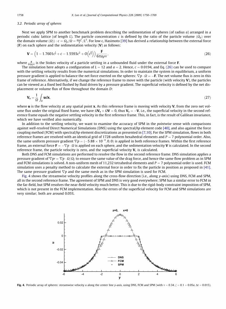
3.2. Periodic array of spheres

Next we apply SPM to another benchmark problem describing the sedimentation of spheres (of radius a) arranged in aperiodic cubic lattice (of length L). The particle concentration c is defined by the ratio of the particle volume ðXpÞ overthe domain volume ðXÞÞ : c ¼ Xp=X ¼ 4pa3

3 =L3. For low c, Hasimoto [39] has derived a relationship between the external force(F) on each sphere and the sedimentation velocity (V) as follows:

Fig. 4.

V ¼ 1� 1:7601c13 þ c � 1:5593c2 þ O c

83

� �� F6paqm

; ð26Þ

where F6paqm is the Stokes velocity of a particle settling in a unbounded fluid under the external force F.

The simulation here adopts a configuration of L ¼ 12 and a ¼ 2. Hence, c ¼ 0:0194, and Eq. (26) can be used to comparewith the settling velocity results from the numerical simulations. In order to maintain the system in equilibrium, a uniformpressure gradient is applied to balance the net force exerted on the spheres: rp �X ¼ �F. The net volume flux is zero in thisframe of reference. Alternatively, if we change the reference frame to move with the particle (with velocity V), the particlescan be viewed as a fixed bed flushed by fluid driven by a pressure gradient. The superficial velocity is defined by the net dis-placement or volume flux of flow throughout the domain D:

Vs ¼1X

ZD

udx; ð27Þ

where u is the flow velocity at any spatial point x. As this reference frame is moving with velocity V, from the zero net vol-ume flux under the original fixed frame, we have XVs þXV ¼ 0, thus Vs ¼ �V, i.e., the superficial velocity in the second ref-erence frame equals the negative settling velocity in the first reference frame. This, in fact, is the result of Galilean invariance,which we have verified also numerically.

In addition to the settling velocity, we want to examine the accuracy of SPM in the pointwise sense with comparisonsagainst well-resolved Direct Numerical Simulations (DNS) using the spectral/hp element code [40], and also against the forcecoupling method (FCM) with spectral/hp element discretizations as presented in [7,10]. For the SPM simulation, flows in bothreference frames are resolved with an identical grid of 1728 uniform hexahedral elements and P ¼ 7 polynomial order. Also,the same uniform pressure gradientrp ¼ ð�5:88� 10�4;0;0Þ is applied in both reference frames. Within the first referenceframe, an external force F ¼ �rp �X is applied on each sphere, and the sedimentation velocity V is calculated. In the secondreference frame, the particle velocity is zero, and the superficial velocity Vs is calculated.

Both DNS and FCM simulations are performed to resolve the flow in the second reference frame. DNS simulation applies apressure gradient ofrp0 ¼ rp �X=Xf to ensure the same value of the drag force, and hence the same flow problem as in SPMand FCM simulations is solved. A non-uniform mesh of 11,232 tetrahedral elements and P ¼ 7 polynomial order is used. FCMsimulation uses a penalty method to calculate the external force in order to fix the particle in position as proposed in [41].The same pressure gradient rp and the same mesh as in the SPM simulation is used for FCM.

Fig. 4 shows the streamwise velocity profiles along the cross-flow direction (i.e., along y-axis) using DNS, FCM and SPM,all in the second reference frame. The agreement of SPM and DNS is very good everywhere; SPM has a similar error to FCM inthe far-field, but SPM resolves the near-field velocity much better. This is due to the rigid-body constraint imposition of SPM,which is not present in the FCM implementation. Also the errors of the superficial velocity for FCM and SPM simulations arevery similar; both are around 0.05%.

y

u

-6 -4 -2 0 2 4 6

-0.04

-0.02

0

0.02

DNSFCMSPM

z=0, x=0

Periodic array of spheres: streamwise velocity u along the center line y-axis, using DNS, FCM and SPM (with m ¼ 0:34; n ¼ 0:1 ¼ 0:05a;Dt ¼ 0:015).

Δt

V er

V er

0 0.01 0.020

1

2

3

4

5

6

(νΔt)0.5/ξ0.6 0.8 1 1.2

0

1

2

3

4

5

6 3 ν0,ξ0, (I)3 ν0,ξ0/2, (I)

ν0,ξ0, (I)3 ν0,ξ0/2, (II)

Fig. 5. SPM for a periodic array of spheres: percentage error in settling velocity Ver versus time step Dt (left) and versusffiffiffiffiffiffiffiffimDtp

=n (right), for two values ofviscosity m and for two values of the interface thickness n. (LEGEND NOTE: ‘m0’: m0 ¼ 0:34; ‘n0’: n0 ¼ 0:1 ¼ 0:05a; ‘(I)’: simulation done in the first referenceframe to calculate V; ‘(II)’: simulation done in the second reference frame with fixed spheres, �Vs calculated to substitute V).


The error plots in Fig. 5 confirm the conclusions of the last subsection, namely that the SPM modeling error is a function ofmDt and n, and the optimum time step size ðDtÞo is determined by the balance of the Stokes layer d ¼ 2:76


and the effec-tive smooth interface thickness le. We find from the above data that le � 2:07n for sufficiently small nðn ¼ 0:025aÞ, which isthe same as the result we obtained for the Couette problem! (We note that le is slightly smaller ðle � 1:97nÞ if we employ alarger value of n, e.g. 0.05a.) Fig. 5 also verifies that the relative difference between the absolute values of the superficialvelocity Vs and the settling velocity V is negligible.

3.3. Rotating sphere at low Reynolds number

Next we investigate the accuracy of SPM in simulating the steady flow induced by a sphere rotating with constant angularvelocity in a viscous incompressible fluid which is at rest at large distances from the sphere. This problem in an open domainhas been treated analytically by Bickley [42], who obtained a second-order approximation for the fluid velocity and pressure,which is quite accurate when the Reynolds number is small. We use this open domain solution as a reference to validate ournumerical simulation results for a finite domain, at Reynolds number less than or equal to 8.0.

The computational domain is ½�p;p� � ½�p;p� � ½�p;p�, with a sphere of radius a ¼ 0:261 centered at the origin and spin-ning with an angular velocity of x ¼ ð0;0;xzÞ. We use this configuration of L=2a ¼ 2p=2a ¼ 12:036 with periodic treatmenton domain boundaries in all three directions to simulate the unbounded flow domain. By the definition of the rotationReynolds number Rew ¼ xza2=m, we set xz ¼ 10:01 and simply change the fluid kinematic viscosity m to obtain different val-ues of Reynolds number, from 0.25 to 8.

The required external torque Text on the sphere to achieve a Reynolds number Rew is estimated from the asymptoticapproximation obtained by Takagi [43]:

2Text=qa5x2z ¼ 16pð1þ f ðRewÞÞ=Rew;

This is a correction to Lamb’s result M ¼ 16p=Rew for Stokes flow [44], and has been confirmed by numerical simulations ofDennis [45] for Re 6 10. Numerical results of the hydrodynamic torque obtained from Eq. (18b) are compared to this givenexternal torque.

For the SPM simulations we used 4096 nonuniform hexahedral elements and a polynomial order of P ¼ 5. The followingindicator function, utilizing the form of (2), was applied:

/ðx; tÞ ¼ 12

tanhf ðx; tÞ

ns

� �þ 1

� �; with f ¼ 1� jxj2=a2; s ¼ a=2: ð28Þ

Compared to the original spherical envelope ((1)), this envelope is slightly different and thus the effective smooth interfacethickness le is slightly different from 2:07n obtained for ((1)). Let us define the effective interface thickness le to be twice thedistance from the particle surface to the spatial point whose concentration function is /e ¼ tanh �2:07=2n

n

� �þ 1

� �=2 ¼ 0:112.

For the original envelopes ((1)), with n ¼ 0:05a ¼ 0:013, le ¼ 2:07n ¼ 0:0269; with the new envelope (28), using the same n,we have le ¼ 2� 0:0127 ¼ 0:0254. The time step size is thus chosen according to the expected optimum time step derived


from 2:76ffiffiffiffiffiffiffiffiffiffiffiffiffiffimðDtÞo

p¼ le. DNS results were obtained using 6600 hexahedral elements with polynomial order P ¼ 7. The FCM

results from [46], which were obtained by a Fourier pseudo-spectral method with 643 grid points for the same domain,are also included for comparison.

We see from Fig. 6 that SPM captures the primary azimuthal velocity quite well, with a maximum pointwise error ofabout 3.2% near the sphere surface (with n ¼ 0:05a). This error goes up to about 4:9% if we use a thicker smooth interface,n ¼ 0:077a. The radial velocity is more challenging to resolve, for it comes from the secondary flow at finite Reynolds num-bers and its magnitude is much smaller than the dominant azimuthal velocity. Fig. 7 shows that there is some effect due tothe periodic boundary conditions as manifested by the difference between the SPM results and the second-order approxi-mate solution [42]. The relative difference in the azimuthal velocity is around 0.00063 on the domain boundaries. Thus,we employ DNS results for a more fair comparison, and the agreement with SPM is good everywhere. We also see thatSPM is resolving the radial velocity much better than FCM near the particle surface ðx=a < 1:3Þ, and it resolves the far-fieldvelocity as well as FCM. By reducing the SPM interface thickness parameter from n ¼ 0:077a to n ¼ 0:05a, the peak pointwiseerror in the radial velocity reduces from about 8.5% to 3.6% for Reynolds number 0.25.

x/a

v/(w

*a)

0 0.5 11 1.5 20

0.2

0.4

0.6

0.8

1

second-order solutionRE=0.25, DNSRE=8.0, DNSRE=0.25, FCMRE=8.0, FCMRE=0.25, SPMRE=8.0, SPM

Fig. 6. Rotating sphere: non-dimensional azimuthal velocity v versus radial distance along the x-axis. Comparison between the second-order approximationsolution and results from DNS, FCM and SPM (with n ¼ 0:05a) for two different Reynolds numbers.

x/a0 2 4 6

u/ (w

*a*R

e)

0

0.002

0.004

0.006

0.008

second-order solutionRE=0.25, DNSRE=8.0, DNSRE=0.25, FCMRE=8.0, FCMRE=0.25, SPMRE=8.0, SPM

Fig. 7. Rotating sphere: Non-dimensional radial velocity u versus radial distance the along x-axis. Comparison between the second-order approximationsolution and results from DNS, FCM and SPM (with n ¼ 0:05a) for two different Reynolds numbers.

u/ (w

*a*R

e)

0

0.002

0.004

0.006

0.008

second-order solutionRE=0.25, DNSRE=0.25, FCMRE=0.25, SPMRE=0.25, SPM(pp)

x/a0 2 4 6

Fig. 8. Rotating sphere at Reynolds number 0.25: non-dimensional radial velocity u versus radial distance along the x-axis. Comparison between thesecond-order approximation solution and results from DNS, FCM, SPM (with n ¼ 0:05a). (LEGEND NOTE: ‘SPM(pp)’: SPM with pp modification step as in Eq.(29).)


With the above SPM setup, we now check the indirect imposition of the no-slip constraint on the sphere boundary by val-idating Eq. (6) on the equator plane z ¼ 0. The right hand side (RHS) is calculated using / from (28), up ¼ x� x anduif ¼ ðx� xÞa3=jxj3 which is the exact Stokes solution for an open domain. The left hand side (LHS) is computed by takingthe numerical gradient of the total velocity. We obtain the relative error between RHS and LHS (in L2-sense) to be around1.1%. By noting that this error mainly comes from the periodic boundary treatment instead of a open domain, and this prob-lem features in sharp transition of the vorticity across the interface, the above test serves as a sufficient verification of theimposition of no-slip boundary constraint in SPM.

Fig. 7 also shows a non-zero radial velocity inside the particle, which is of the same order of magnitude as the peak errorin the radial velocity. This particle-penetrating phenomenon arises from the final updating step Eq. (22), where rpp has anon-zero value even inside the particle. In order to suppress this erroneous velocity we modify (22) to:

c0unþ1 � u�

dt¼ c0

/ðunþ1p � u�Þ

dt� ð1� /Þrpp: ð29Þ

We see from Fig. 8 that the result is satisfying, as this modification ensures the non-penetrating constraint is satisfied strictlyinside the particle as well and this has as a result a further reduction in the error of the radial velocity outside the particle.However, this modification introduces some compressibility inside and on the particle boundary (i.e., /–0), see Eqs. (21a)and (29). Indeed, the numerical results show that the divergence of the total velocityr � unþ1 is slightly larger than the diver-gence of the intermediate velocity r � u� inside the particle, however, both are of comparable magnitude.

3.4. Stokes oscillating plate

Next we study an unsteady problem in order to evaluate the temporal discretization error and how it compares to themodeling error inherent in SPM. To this end, we consider the problem of an infinite plate oscillating in an unbounded fluid.The simulation domain is ½0;1� � ½0;6� � ½0;1�, where y 2 ½0;3� is the solid plate modeled by SPM and the fluid flow is in theinterval y 2 ½3;6�. The plate moves with an oscillating velocity V ¼ ðsinðxtÞ;0;0Þ. The exact solution given in [47] is

uex ¼ ðe�Y=ffiffi2p

sinðT � Y=ffiffiffi2pÞ;0;0Þ;

where Y ¼ y�3ðm=xÞ1=2 and T ¼ xt for our case. We treat the boundary at y ¼ 6 as a Dirichlet boundary using the exact solution;

periodicity is imposed along both the x- and z-directions.We calculate the L2 error of the streamwise velocity in the domain ðy 2 ½0;3�Þ at each time step and then calculate the

mean error after convergence (to a constant-amplitude sine function in time). Here, we specify the fluid kinematic viscosityas m ¼ 1 and the oscillating frequency parameter to be x ¼ 1. SPM simulations are performed on a mesh of 6 non-uniformhexahedral elements with P ¼ 7 polynomial order. Different orders (Je ¼ 1;2 or 3) in time integration for solving the inter-mediate velocity u� are employed.

From Fig. 9, we see that indeed higher time-integration order Je leads to smaller errors beyond the optimum time step sizewhere the temporal discretization error dominates over the SPM modeling error. This behavior, in fact, confirms that the

L2er

-mea

n

0

0.002

0.004

0.006

0.008

0.01

0.012

Δt0 0.002 0.004 0.006

L2er

-mea

n

0

0.016

0.014

0.012

0.01

0.008

0.006

0.004

0.002

Δt0 0.002 0.004 0.006

ξ=0.05, Je=1ξ=0.05, Je=2ξ=0.08, Je=1ξ=0.08, Je=2ξ=0.02, Je=1ξ=0.02, Je=2

ξ=0.05, Je=1ξ=0.05, Je=2ξ=0.05, Je=3

Fig. 9. Oscillating plate: Mean L2 error ðL2er�meanÞ versus time step size Dt for different order Je (left) and different interface thickness parameter n (right).


temporal error has two contributions: (1) the SPM modeling error, which is a function of mDt and n, and (2) the discretizationerror from the time-integration scheme we use for the intermediate velocity field solving Eqs. (13)–(15) and (17); the seconderror scales as ðmDtÞJe for unsteady problems (see details in [35]). With regards to the effect of the profile thickness n, ourresults suggest that larger thickness n and higher order Je would lead to larger optimum time step ðDtÞo, which is clearlyadvantageous in production simulations.

4. Flow past complex-shaped particles

So far we have modeled particles with simple shapes but in this section we employ the new general envelopes (Eq. (2)) tomodel flow past complex-shaped particles. SPM is advantageous in that it does not require complex meshes around the par-ticle surfaces, as the computational domain is the entire domain including particle domains. The way it represents the com-plex-shaped particles is rather straightforward. As long as we know the surface function of the particles or we have thecoordinates of a sufficient number of points on the particle surfaces, we can obtain the concentration field / representingthe particles, and then solve the governing equations for the flow. In the following we examine the accuracy of SPM for ellip-soidal and biconcave particles.

4.1. Stokes flow past an ellipsoid

We first study ellipsoidal particles, specifically spheroids. Similar to what we employed for the rotating sphere, here toowe use an indicator function utilizing Eq. (2) with

f ¼ 1� ðx2=a2 þ y2=b2 þ z2=c2Þ; and s ¼ffiffiffiffiffiffiffiffiabc3p

=2;

where a; b; c are the semi-axes of the ellipsoid centered at the origin.With this concentration function we apply SPM to the problem of Stokes flow past a spheroid (aligned with the flow) be-

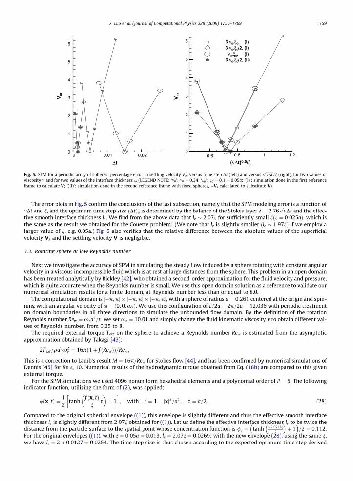
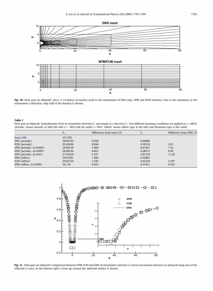
tween two infinite parallel walls. The simulation domain is ½80;80� � ½�3:3333;10� � ½�20;20� with y ¼ �3:3333 and y ¼ 10to be the walls. Periodicity is imposed in both x- and z-directions. A spheroid with semi-axes of a ¼ 2; b ¼ 1 and c ¼ 1 is cen-tered at the origin with its long axis aligned with x-axis. A uniform pressure gradient of rp ¼ ð0:06075;0;0Þ is applied todrive the flow. Thus, the flow far from the ellipsoid can be modeled as a fully developed Poiseuille flow driven by this pres-sure gradient, and correspondingly the centerline velocity is Ucl ¼ 1:35. Based on these values, we obtain from Table 7–5.1 in[48] the ‘‘exact” drag force ðFxÞex ¼ 29:1765 for a fixed ellipsoid immersed in an infinite Poseuille flow. We use this force va-lue as the ‘‘exact” drag force to compare against our SPM results on a finite computational domain.

In the SPM simulation we use 4560 rectilinear elements with polynomial order P ¼ 3, with finer resolution around thespheroid (see Fig. 10). We choose the interface thickness to be n ¼ 0:1b.

For comparison, we have also performed both DNS and FCM simulations. In FCM we employed the same mesh as in theSPM simulation (i.e., 4560 elements with P ¼ 3), and we computed the hydrodynamic force and torque using a penalty meth-od as in [41]. DNS simulation employs 7168 hexahedral elements with polynomial order P ¼ 4. The meshes, displaying theelements only, are shown in Fig. 10.

We have summarized the results of our simulations in Table 1. It shows that for this value of n, the optimum time stepsize is around 0.005, which, in fact, is the value expected from the balance of the Stokes layer thickness d and the effectiveinterface thickness le, i.e., d ¼ 2:76

ffiffiffiffiffiffiffiffiffiffiffiffiffiffimðDtÞo

p¼ le (obtained from the Couette problem). For n ¼ 0:1b, we obtain the effective

interface thickness in x, y and z direction as ðleÞx ¼ 2� 0:1529; ðleÞy ¼ ðleÞz ¼ 2� 0:07645. Let us define the total effective

y

SPM/FCM mesh

x

y

0 20 40 60 80

x0 20 40 60 80

0

5

10

0

5

10

DNS mesh

Fig. 10. Flow past an ellipsoid: slices (z = 0 plane) of meshes used in the simulations of DNS (top), SPM and FCM (bottom). Due to the symmetry in thestreamwise x-direction, only half of the domain is shown.

Table 1Flow past an ellipsoid: hydrodynamic force in streamwise direction Fx and torque in z-direction Tz . Two different boundary conditions are applied at x = ±80.0:‘periodic’ means periodic at both the inlet x = �80.0 and the outlet x = 80.0; ‘inflow’ means inflow type at the inlet and Neumann type at the outlet.

Fx Difference from exact (%) Tz Difference from DNS (%)

Exact [48] 29.1765DNS (periodic) 28.89703 0.958 4.29880FCM (periodic) 29.43436 0.884 4.38510 2.01SPM (periodic, Dt=0.003) 29.90128 2.484 4.61497 7.35SPM (periodic, Dt=0.005) 28.98194 0.667 4.28673 0.28SPM (periodic, Dt=0.01) 27.55520 5.557 3.81726 11.20DNS (inflow) 29.61001 1.486 4.32863FCM (inflow) 29.62734 1.545 4.42328 2.187SPM (inflow, Dt=0.005) 29.170 0.022 4.31411 0.335

x

u

0 20 40 60 80-0.2

0

0.2

0.4

0.6

0.8

SPM

FCM

DNS

x

u

0 1 2 3 4 5 6 7

0

0.2

0.4

0.6

0.8

1

1

Fig. 11. Flow past an ellipsoid: Comparison between SPM, FCM and DNS of streamwise velocity (u) versus streamwise distance (x) along the long axis of theellipsoid (x-axis). In the bottom right a close-up around the spheroid surface is shown.


SPM

FCM

DNS

0

y-2 0 82 4 6 1

u

0

0.5

1

y-3 -2.5 -2 -1.5 -1 -0.5

u 0.1

0.2

Fig. 12. Flow past an ellipsoid: Comparison between SPM, FCM and DNS of streamwise velocity (u) versus inter-wall distance (y) along the short axis of theellipsoid (y-axis). In the bottom right a close-up around the spheroid surface is shown.

y

u

0 10

0

0.2

0.4

0.6

0.8

1

1.2

SPMFCMDNS

5

Fig. 13. Flow past an ellipsoid: Comparison between SPM, FCM and DNS of streamwise velocity (u) versus inter-wall distance (y) along the tangential lineðz ¼ 0; x ¼ �2Þ.


interface thickness as the geometric mean of all three directions to obtain le ¼ffiffiffiffiffiffiffiffiffiffiffiffiffiffiffiffiffiffiffiffiffiffiffiffiffiffiðleÞxðleÞyðleÞz3

q¼ 2� 0:09632, and hence

ðDtÞo ¼ le2:76

2=m ¼ 0:00524, which agrees with the SPM simulation results. Table 1 also shows that the boundary treatment

at the inlet and outlet has certain effects in the numerical results.Next, we compare the SPM results against DNS and FCM results for the same conditions (with periodic boundary treat-

ment) in the pointwise sense, e.g., we compare velocity profiles at different locations, in Figs. 11–13. The results indicate thatif we choose the time step wisely and the interface thickness reasonably, SPM resolves the near velocity fields better thanFCM while in far-field it is comparable to FCM.

4.2. Flow past a biconcave particle

Biconcave shaped particles resemble red blood cells, so we are interested to assess the accuracy of SPM for flow past asingle particle tilted with respect to the flow direction. The concentration function for biconcave is derived from (2) usingthe surface function f given in [49]:

f ðx; tÞ ¼ jxj � ða� bÞ sinq hþ b; and s ¼ 1

where a; b are the semi-axes of the biconcave, h is the orientation angle as h ¼ arccosðxI=jxjÞ, and xI is the projection of x ontothe symmetry axis of the biconcave. We simulate the steady Stokes flow past a tilted biconcave particle between two walls.


The simulation domain is ½�6;6� � ½�4;4� � ½�6;6�, with a particle of a ¼ 2:22; b ¼ 0:62 centered at the origin and tilted inthe z-direction by an angle of �p=4. Two walls are located at y ¼ 4, and periodicity is imposed along the x- and z-directions.A pressure gradientrp ¼ ð0:05;0;0Þ is prescribed to drive the flow. As the biconcave is tilted, both drag force Fx and lift forceFy are expected.

The SPM simulation uses 7200 nonuniform hexahedral elements with fourth-order polynomials, while DNS uses 50941tetrahedral elements and a polynomial order of P ¼ 8; the meshes (elements only) are shown in Fig. 14. Compared to theDNS mesh, the rectilinear mesh for SPM is much simpler and more manageable.

Typical results for velocity profiles at different locations are shown in Figs. 15–17. We could not obtain FCM results forthis complex shape so we compare against the DNS results with spectral element method. The agreement is very good andcomparable to the simple shaped particle simulations we considered in previous sections.

x

y

-6 -4 -2 0-4

-2

0

2

4SPM mesh

2 4 6

DNS mesh

Fig. 14. Flow past a biconcave particle: slices (z = 0 plane) of meshes used in the simulations of DNS (top) and SPM (bottom), for the same computationaldomain.

x

y

-5 0 5-4

-2

0

2

4

6

8

10

12

140.9

0.5

0.1

φ

x

u

-6 -4 -2 0 2 4 60

0.05

0.1

0.15DNSSPM

Fig. 15. Flow past a biconcave particle: Left: 2D streamlines and concentration function contour in z = 0 plane by SPM; Right: comparison between SPM andDNS: streamwise velocity (u) versus streamwise distance (x) along the center line: z = 0, y = 0.

0.9

0.5

0.1

zu

-6 -4 -2 0 2 4 60

0.05

0.1

0.15

0.2

0.25

0.3

0.35

DNS

SPM

x

z

-5 0 5

-5

0

5

10

15φ

Fig. 16. Flow past a biconcave particle: Left: 2D streamlines and concentration function contours at the y = 0 plane by SPM. Right: comparison between SPMand DNS: streamwise velocity (u) versus depth distance (z) along the center line: y ¼ 0; x ¼ 0.

x

v

-5 0

.025

-0.02

.015

-0.01

.005

0

z=0, y=0

x

v

-5 0

-0.04

-0.03

-0.02

-0.01

0

0.01DNSSPM

z=0, y=1

5 5

Fig. 17. Flow past a biconcave particle: Inter-wall velocity (v) versus streamwise distance (x). Left: along the center line z ¼ 0; y ¼ 0. Right: along the linez ¼ 0; y ¼ 1.


5. Two interacting spheres

We employ SPM to study the pairwise interaction between two spheres rising in a vertical channel at low Reynolds num-ber. We check if the SPM simulation can reproduce the drafting–kissing–tumbling (DKT) scenario observed in the experi-ments [50,51]. The numerical results are compared with both the experimental and FCM results presented in [52].

The experimental setup was a vertical channel of ½0;150� � ½�5;5� � ½�50;50� (all in mms). The channel was filled with amixture of glycerol and water with density qf ¼ 1:094 g=cm3. Two spheres with radius a ¼ 1 mm and density

Y

YX X

-3

-3

-2

-2

-1

-1

0

0

1

1

2

2

3

3

0 0

20 20

40 40

60 60

80 80

100 100

0

20

40

60

80

100

EXP,p1

EXP,p2

FCM,p1

FCM,p2

SPM,p1

SPM,p2

Z

Z

X X

-5

-5

-4

-4

-3

-3

-2

-2

-1

-1

0

0

1

1

2

2

3

3

0

20

40

60

80

100

EXP,p1

EXP,p2

FCM,p1

FCM,p2

SPM,p1

SPM,p2

a b

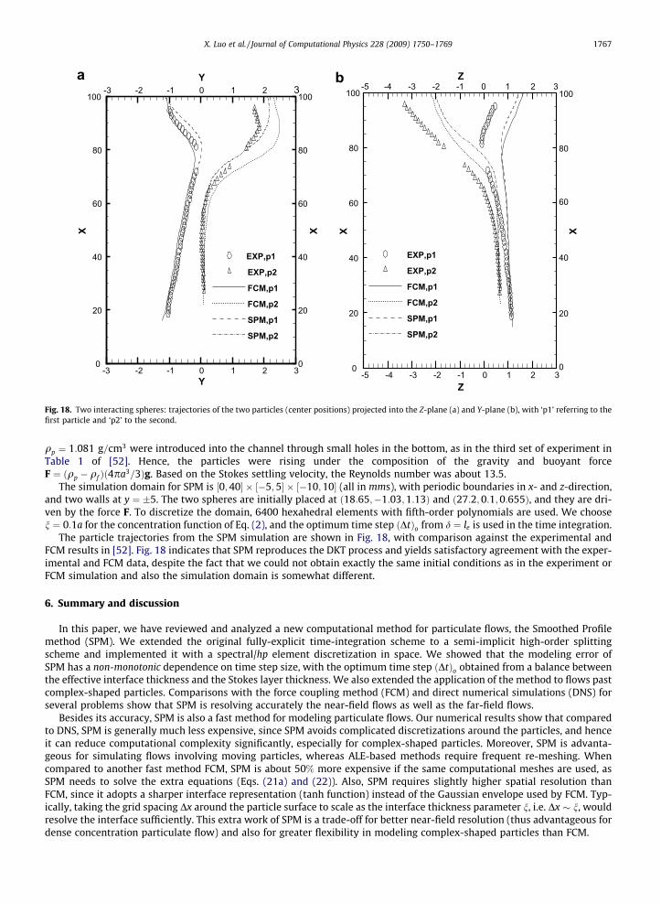
Fig. 18. Two interacting spheres: trajectories of the two particles (center positions) projected into the Z-plane (a) and Y-plane (b), with ‘p1’ referring to thefirst particle and ‘p2’ to the second.


qp ¼ 1:081 g=cm3 were introduced into the channel through small holes in the bottom, as in the third set of experiment inTable 1 of [52]. Hence, the particles were rising under the composition of the gravity and buoyant forceF ¼ ðqp � qf Þð4pa3=3Þg. Based on the Stokes settling velocity, the Reynolds number was about 13.5.

The simulation domain for SPM is ½0;40� � ½�5;5� � ½�10;10� (all in mms), with periodic boundaries in x- and z-direction,and two walls at y ¼ 5. The two spheres are initially placed at ð18:65;�1:03;1:13Þ and ð27:2;0:1;0:655Þ, and they are dri-ven by the force F. To discretize the domain, 6400 hexahedral elements with fifth-order polynomials are used. We choosen ¼ 0:1a for the concentration function of Eq. (2), and the optimum time step ðDtÞo from d ¼ le is used in the time integration.

The particle trajectories from the SPM simulation are shown in Fig. 18, with comparison against the experimental andFCM results in [52]. Fig. 18 indicates that SPM reproduces the DKT process and yields satisfactory agreement with the exper-imental and FCM data, despite the fact that we could not obtain exactly the same initial conditions as in the experiment orFCM simulation and also the simulation domain is somewhat different.

6. Summary and discussion

In this paper, we have reviewed and analyzed a new computational method for particulate flows, the Smoothed Profilemethod (SPM). We extended the original fully-explicit time-integration scheme to a semi-implicit high-order splittingscheme and implemented it with a spectral/hp element discretization in space. We showed that the modeling error ofSPM has a non-monotonic dependence on time step size, with the optimum time step ðDtÞo obtained from a balance betweenthe effective interface thickness and the Stokes layer thickness. We also extended the application of the method to flows pastcomplex-shaped particles. Comparisons with the force coupling method (FCM) and direct numerical simulations (DNS) forseveral problems show that SPM is resolving accurately the near-field flows as well as the far-field flows.

Besides its accuracy, SPM is also a fast method for modeling particulate flows. Our numerical results show that comparedto DNS, SPM is generally much less expensive, since SPM avoids complicated discretizations around the particles, and henceit can reduce computational complexity significantly, especially for complex-shaped particles. Moreover, SPM is advanta-geous for simulating flows involving moving particles, whereas ALE-based methods require frequent re-meshing. Whencompared to another fast method FCM, SPM is about 50% more expensive if the same computational meshes are used, asSPM needs to solve the extra equations (Eqs. (21a) and (22)). Also, SPM requires slightly higher spatial resolution thanFCM, since it adopts a sharper interface representation (tanh function) instead of the Gaussian envelope used by FCM. Typ-ically, taking the grid spacing Dx around the particle surface to scale as the interface thickness parameter n, i.e. Dx � n, wouldresolve the interface sufficiently. This extra work of SPM is a trade-off for better near-field resolution (thus advantageous fordense concentration particulate flow) and also for greater flexibility in modeling complex-shaped particles than FCM.


Although in the previous papers SPM has only been applied to zero and low Reynolds number flow problems ðRe < 20Þ,extensions to moderate and high Reynolds number flows are feasible. For higher Reynolds number flow, both the Stokeslayer thickness ðd � 2:76


Þ and the boundary layer thickness ðdbl � x=ffiffiffiffiffiffiRepÞ become thinner. For best modeling accuracy,

we need to choose a time step close to the optimum size ðDtÞo which balances the effective interface thickness ðle ¼ 2:07nÞand the Stokes layer thickness (d), i.e., le ¼ d as stated in subSection 3.1. In addition, we need to make sure that the smoothinterface adequately resolves the boundary layer (i.e., le < dbl), which is usually automatically satisfied in our simulations ifthe optimum time step ðDtÞo is used and it is below the CFL limit. Our SPM simulation results for moderate Reynolds numberflow around a 2D circular cylinder reveal good agreement with the experimental results of Hammache et al. [53]; e.g., therelative error in the Strouhal number is about 2.2% and 0.9%, respectively, for Re ¼ 100 and 150. Also, the SPM results ofvelocity profiles averaged over one Strouhal period (not shown here for brevity) at different locations are in excellent agree-ment with the DNS results for Re ¼ 100 � 200.

SPM can be readily extended to many interacting particles as suggested by our simulations of two particles. However, aproper contact force model is required to prevent the particles from overlapping. Furthermore, SPM is a good candidate formultiscale modeling of colloidal suspensions, and the initial results in [54] based on a similar modeling method areencouraging.

Acknowledgments

This work was supported by National Science Foundation. Special thanks are given to Prof. Don Liu who provided the ori-ginal FCM-spectral element code, and to Kyongmin Yeo who contributed the FCM results for the rotating sphere section. Wewould also like to thank Dr. Sune Lomholt for his original data of two interacting particles.

References

[1] Y. Nakayama, R. Yamamoto, Simulation method to resolve hydrodynamic interactions in colloidal dispersions, Phys. Rev. E 71 (2005) 036707.[2] H.H. Hu, Direct simulation of flows of solid–liquid mixtures, Int. J. Multiphase Flow 22 (2) (1996) 335–352.[3] H.H. Hu, N.A. Patankar, M.Y. Zhu, Direct numerical simulations of fluid–solid systems using the arbitrary Lagrangian–Eulerian technique, J. Comput.

Phys. 169 (2) (2001) 427–462.[4] R. Glowinski, T.W. Pan, T.I. Hesla, D.D. Joseph, A distributed Lagrange multiplier/fictitious domain method for particulate flow, Int. J. Multiphase Flow

25 (1999) 755–794.[5] R. Glowinski, T.W. Pan, T.I. Hesla, D.D. Joseph, J. Periaux, A fictitious domain approach to the direct numerical simulation of incompressible viscous flow

past moving rigid bodies: application to particulate flow, J. Comput. Phys. 169 (2001) 363–426.[6] N.A. Patankar, P. Singh, D.D. Joseph, R. Glowinski, T.W. Pan, A new formulation of the distributed Lagrange multiplier/factious domain method for

particulate flows, Int. J. Multiphase Flow 26 (2000) 1509–1524.[7] M.R. Maxey, B.K. Patel, Localized force representations for particles sedimenting in Stokes flow, Int. J. Multiphase Flow 27 (9) (2001) 1603–1626.[8] S. Lomholt, M.R. Maxey, Force-coupling method for particulate two-phase flow: Stokes flow, J. Comput. Phys. 184 (2003) 381–405.[9] D. Liu, M.R. Maxey, G.E. Karniadakis, A fast method for particulate microflows, J. Microelectromech. Syst. 11 (2002) 691–702.

[10] D. Liu, M.R. Maxey, G.E. Karniadakis, FCM-spectral element method for simulating colloidal micro-devices, Comput. Fluid Solid Mech. 2003 (2003)1413–1416.

[11] C.S. Peskin, Flow patterns around heart valves: a numerical method, J. Comput. Phys. 10 (1972) 252.[12] C.S. Peskin, Numerical analysis of blood flow in the heart, J. Comput. Phys. 25 (1977) 220.[13] A. Fogelson, C. Peskin, A fast numerical method for solving the three-dimensional stokes equation in the presence of suspended particles, J. Comput.

Phys. 79 (1988) 50–69.[14] R.P. Beyer, R.J. LeVeque, Analysis of a one-dimensional model for the immersed boundary method, SIAM J. Numer. Anal. 29 (2) (1992) 332–364.[15] M.C. Lai, C.S. Peskin, An immersed boundary method with formal second-order accuracy and reduced numerical viscosity, J. Comput. Phys. 160 (2000)

705–719.[16] D. Goldstein, R. Handler, L. Sirovich, Modeling a no-slip boundary with an external force field, J. Comput. Phys. 105 (1993) 354–366.[17] E. Fadlun, R. Verzicco, P. Orlandi, J. Mohd-Yusof, Combined immersed boundary finite-difference methods for three-dimensional complex flow

simulations, J. Comput. Phys. 161 (2000) 35–60.[18] M. Uhlmann, An immersed boundary method with direct forcing for the simulation of particulate flows, J. Comput. Phys. 209 (2) (2005) 448–476.[19] R.J. LeVeque, Z. Li, The immersed interface method for elliptic equations with discontinuous coefficients and singular sources, SIAM J. Numer. Anal. 31

(1994) 1019–1044.[20] R.J. LeVeque, Z. Li, Immersed interface methods for Stokes flow with elastic boundaries or surface tension, SIAM J. Sci. Comput. 18 (3) (1997) 709–735.[21] Z. Li, M.C. Lai, The immersed interface method for the Navier–Stokes equations with singular forces, J. Comput. Phys. 171 (2) (2001) 822–842.[22] L. Lee, R.J. LeVeque, An immersed interface method for incompressible Navier–Stokes equations, SIAM J. Sci. Comput. 25 (2003) 832–856.[23] K. Kim, Y. Nakayama, R. Yamamoto, A smoothed profile method for simulating charged colloidal dispersions, Comput. Phys. Commun. 169 (1–3) (2005)

104–106.[24] R. Yamamoto, Y. Nakayama, K. Kim, A method to resolve hydrodynamic interactions in colloidal dispersions, Comput. Phys. Commun. 169 (1–3) (2005)

301–304.[25] Y. Nakayama, K. Kim, R. Yamamoto, Hydrodynamic effects in colloidal dispersions studied by a new efficient direct simulation, in: Flow Dynamics,

American Institute of Physics Conference Series, vol. 832, 2006, pp. 245–250.[26] Y. Nakayama, K. Kim, R. Yamamoto, Simulating (electro)hydrodynamic effects in colloidal dispersions: smoothed profile method (cond-mat/0601322).[27] K. Kim, Y. Nakayama, R. Yamamoto, Direct numerical simulations of electrophoresis of charged colloids (cond-mat/0601534).[28] R. Yamamoto, K. Kim, Y. Nakayama, Strict simulations of non-equilibrium dynamics of colloids, Colloid Surf. A: Physicochem. Eng. Asp. 311 (1–3)

(2007) 42–47.[29] H.N.O.S. Takagia, Z. Zhangb, A. Prosperetti, PHYSALIS: a new method for particle simulation Part II: Two-dimensional Navier–Stokes flow around

cylinders, J. Comput. Phys. 189 (2) (2003) 493–511.[30] H. Huang, S. Takagi, PHYSALIS: a new method for particle flow simulation, Part III: Convergence analysis of two-dimensional flows, J. Comput. Phys.

189 (2) (2003) 493–511.[31] Y. Nakayama, K. Kim, R. Yamamoto, Simulating (electro)hydrodynamic effects in colloidal dispersions: smoothed profile method, Eur. Phys. J. E 26

(2008) 361–368.[32] K. Kim, Y. Nakayama, R. Yamamoto, Direct numerical simulations of electrophoresis of charged colloids, Phys. Rev. Lett. 96 (2006) 208302.


[33] D. Funaro, D. Gottlieb, A new method of imposing boundary conditions in pseudospectral approximations of hyperbolic equations, Math. Comput. 51(184) (1988) 599–613.

[34] J.S. Hesthaven, D. Gottlieb, A stable penalty method for the compressible Navier–Stokes equations: I. Open boundary conditions, SIAM J. Sci. Comput.17 (3) (1996) 579.

[35] G.E. Karniadakis, M. Israeli, S.A. Orszag, High-order splitting methods for the incompressible Navier–Stokes equations, J. Comput. Phys. 97 (1991) 414.[36] G.E. Karniadakis, S.J. Sherwin, Spectral/hp Element Methods for CFD, Oxford University Press, New York, 1999.[37] D. Xiu, G.E. Karniadakis, A semi-Lagrangian high-order method for Navier–Stokes equations, J. Comput. Phys. 172 (2001) 658–684.[38] P.K. Kundu, I.M. Cohen, Fluid Mechanics, second ed., Academic Press, 2002 (Chapter 9, pp. 282–288).[39] H. Hasimoto, On the periodic fundamental solutions of the Stokes equation and their application to viscous flow past a cubic array of spheres, J. Fluid

Mech. 5 (1959) 317–328.[40] R.M. Kirby, T.C. Warburton, S.J. Sherwin, A. Beskok, G.E. Karniadakis, The Nektar code: dynamic simulations without re-meshing, in: Proceedings of the

2nd International Conference on Computational Technologies for Fluid/Thermal/Chemical Systems with Industrial Applications, August 1–5, 1999.[41] D. Liu, M.R. Maxey, G.E. Karniadakis, Modeling and optimization of colloidal micro-pumps, J. Micromech. Microeng. 14 (9) (2004) 567–575.[42] W.G. Bickley, On the secondary flow due to a sphere rotating in a viscous fluid, Talbot Bull. Lond. Math. Soc. 5 (1973) 349–354.[43] H. Takagi, Viscous flow induced by slow rotation of a sphere, J. Phys. Soc. Jpn. 42 (1) (1977) 319–325.[44] H. Lamb, Hydrodynamics, Cambridge University Press, 1932. pp. 558–559.[45] S.C.R. Dennis, S.N. Singh, D.B. Ingham, The steady flow due to a rotating sphere at low and moderate Reynolds number, J. Fluid Mech. 101 (1980) 257–

279.[46] E. Climent, K. Yeo, M.R. Maxey, G.E. Karniadakis, Dynamic self-assembly of spinning particles, J. Fluid Eng. 129 (2007) 379–387.[47] R.L. Panton, Incompressible Fluid Flow, Wiley, New York, 1984.[48] J. Happel, H. Brenner, Low Reynolds Number Hydrodynamics, Prentice-Hall, 1965 (Chapter 7, pp. 331–337).[49] J.Q. Lu, P. Yang, X.H. Hu, Simulations of light scattering from a biconcave red blood cell using the finite-difference time-domain method, J. Biomed. Opt.

10 (2) (2005) 024022.[50] K.O.L.F. Jayaweera, B.J. Mason, G.W. Slack, The behaviour of clusters of spheres falling in a viscous fluid Part 1. Experiment, J. Fluid Mech 20 (1964) 121–

128.[51] A. Fortes, D. Joseph, T. Lundgren, Nonlinear mechanics of fluidization of beds of spherical particles, J. Fluid Mech. 177 (1987) 467–483.[52] S. Lomholt, B. Stenum, M. Maxey, Experimental verification of the force-coupling method for particulate flows, Int. J. Multiphase Flow 28 (2002) 225–

246.[53] M. Hammache, M. Gharib, An experimental study of the parallel and oblique vortex shedding from circular cylinders, J. Fluid Mech. Dig. Arch. 232

(1991) 567–590.[54] M. Fujita, Y. Yamaguchi, Multiscale simulation method for self-organization of nanoparticles in dense suspension, J. Comput. Phys. 223 (1) (2007) 108–

120.

Documents

Journal of Computational Physics - brown.edu · Received in revised form 30 ... Journal of Computational Physics 228 (2009) ... IBM in that the force distribution effectively imposes