Embed Size (px)
Citation preview
Journal of Computational Physics 230 (2011) 1319–1334
Contents lists available at ScienceDirect
Journal of Computational Physics
journal homepage: www.elsevier .com/locate / jcp
Adaptive artificial boundary condition for the two-level Schrödingerequation with conical crossings
Houde Han ⇑, Zhiwen ZhangDepartment of Mathematical Sciences, Tsinghua University, Beijing 100084, PR China
a r t i c l e i n f o
Article history:Received 14 June 2010Received in revised form 2 November 2010Accepted 2 November 2010Available online 11 November 2010
Keywords:Schrödinger equationConical crossingsSurface hopping methodArtificial boundary conditionOperator splitting methodUnbounded domain
0021-9991/$ - see front matter � 2010 Elsevier Incdoi:10.1016/j.jcp.2010.11.004
⇑ Corresponding author. Tel.: +88 10 6278 8979.E-mail addresses: [email protected] (H
a b s t r a c t
In this paper, we present an adaptive approach to design the artificial boundary conditionsfor the two-level Schrödinger equation with conical crossings on the unbounded domain.We use the windowed Fourier transform to obtain the local wave number information inthe vicinity of artificial boundaries, and adopt the operator splitting method to obtain anadaptive local artificial boundary condition. Then reduce the original problem into an ini-tial boundary value problem on the bounded computational domain, which can be solvedby the finite difference method. By this numerical method, we observe the surface hoppingphenomena of the two-level Schrödinger equation with conical crossings. Several numer-ical examples are provided to show the accuracy and convergence of the proposed method.
� 2010 Elsevier Inc. All rights reserved.
1. Introduction
The numerical solution of partial differential equations on unbounded domain arises in a large variety of applications inscience and engineering areas. A typical example concerned in this paper is the two-level Schrödinger equation with conicalcrossings as follow:
i@tWðx; tÞ ¼ �Dx þ VðxÞð ÞWðx; tÞ; ðx; tÞ 2 R2 � Rþ; ð1:1Þ
Wðx;0Þ ¼ W0ðxÞ 2 L2ðR2;C2Þ: ð1:2Þ
Here x = (x,y) 2 R2 and W(x, t) = [w1(x, t), w2(x, t)]T 2 C2 is the vector wave function. The kinetic operator Dx is defined by
Dx ¼@xx þ @yy 0
0 @xx þ @yy
� �ð1:3Þ
and the potential operator V(x) is a real symmetric potential matrix, defined by
VðxÞ ¼ 12ðtrVðxÞÞIþ
v1ðxÞ v2ðxÞv2ðxÞ �v1ðxÞ
� �; ð1:4Þ
. All rights reserved.
. Han), [email protected] (Z. Zhang).
1320 H. Han, Z. Zhang / Journal of Computational Physics 230 (2011) 1319–1334
where I is a 2 � 2 identity matrix. The matrix V(x) has eigenvalues
Kð�Þ ¼ trVðxÞ �ffiffiffiffiffiffiffiffiffiffiffiffiffiffiffiffiffiffiffiffiffiffiffiffiffiffiffiffiffiffiffiffiffiffiv1ðxÞ2 þ v2ðxÞ2
q;
which are called the potential energy surfaces in chemistry literatures [7,10,12,38]. Two potential energy surfaces are calledcrossing at a point x* 2 R2 if K+(x*) = K�(x*). Such a crossing is called conical if the vectors rxv1(x*) and rxv2(x*) are linearlyindependent. If all the crossings are conical crossings, the crossing set S = {x 2 R2jK+(x) = K�(x)} is a submanifold of codimen-sion two in R2.
There are a lot of studies on the numerical solution of the time-dependent two-level Schrödinger equation with conicalcrossings on the bounded domain. For example, Kammerer, Lasser, Teufel et al. analyzed the propagation through conicalsurface crossings using the Wigner transform and Wigner measures [8,9] and proposed a rigorous surface hopping methodbased on the semiclassical limit of the time-dependent Born–Oppenheimer approximation, namely, the system of linearLiouville equations, see [10,11,7]. In [12], Jin et al. proposed an Eulerian surface hopping method for the two-level Schröding-er equation with conical crossings. However, when one wants to numerically solve the time-dependent two-level Schröding-er equation on the unbounded domain, these methods will face essential difficulties. Since the standard finite elementmethod or finite difference method cannot be used directly on the unbounded domain.
The artificial boundary condition (ABC) method is a powerful approach to reduce the problems defined on the unboundeddomain to a bounded domain, see [14,35,36]. In general, the artificial boundary conditions can be classified into implicitboundary conditions and explicit boundary conditions including global, also called non-local ABC, local ABC and discreteABC [14]. For the last 30 years, many mathematicians have made great contributions in this subject, such as, [1,2] for hyper-bolic wave equations, [3,4] for parabolic equations and [5,6] for elliptic equations, which makes the artificial boundary con-dition method for the linear partial differential equations on the unbounded domain becomes a well-developed method.
In the case of the linear Schrödinger equation, Antoine and Besse [23] obtained a non-reflecting boundary conditions forthe one-dimensional Schrödinger equation. Then Antoine et al. [24] generalized their approach to simulate the two-dimen-sional Schrödinger equation using non-reflecting boundary conditions. Han and Huang [15], Han et al. [16] derived the exactnon-reflecting boundary conditions for two-and three-dimensional Schrödinger equations. Zisowsky [22] studied and de-rived the discrete transparent boundary conditions for systems of Schrodinger equation.
The treatment of the boundary conditions on the artificial boundary for nonlinear equations is difficult in general. Hag-strom and Keller [13] studied some nonlinear elliptic problems by linearizing the equations. Han et al. [17] and Xu et al. [18],discussed the nonlinear Burgers equation and Kardar–Parisi–Zhang equation, respectively. Han and Zhang [19] obtained thelocal artificial boundary conditions for the one-dimensional nonlinear Klein–Gordon equation on unbounded domain.
For the works related to the nonlinear Schrödinger equation, Zheng [26] obtained the global boundary condition using theinverse scattering transform approach for the cubic nonlinear Schrödinger equation in one dimension. Antonie et al. [25]studied the one-dimensional cubic nonlinear Schrödinger equation and constructed several nonlinear integro-differentialartificial boundary conditions. In [27,28], Szeftel designed absorbing boundary conditions for one-dimensional nonlinearwave equation by the potential and the paralinear strategies. Especially, the one-dimensional nonlinear Schrödinger equa-tion was discussed. Recently, Xu and Han [20,21] proposed a split local absorbing boundary (SLAB) method through a time-splitting procedure to design adaptive absorbing boundary conditions for one-and two-dimensional nonlinear Schrödingerequations.
The essential difficulty of the numerical solution to the problem (1.1) and (1.2) involves two parts, the potential V(x) isnonconstant and the physical computational domain is unbounded. In Eq. (1.1), the kinetic operator and potential operatorare coupled together, which makes it is difficult to design the artificial boundary conditions directly. In this paper, we use theoperator splitting method to obtain the local artificial boundary conditions for the two-level Schrödinger equation (1.1) withconical crossings on the unbounded domain. Then reduce the original problem (1.1) and (1.2) into an initial boundary valueproblem on the bounded computational domain, which can be solved by the finite difference method. By this numericalmethod, we can observe the surface hopping phenomena of the two-level Schrödinger equation with conical crossings.
This paper is organized as follows. In Section 2, we propose an adaptive artificial boundary condition for the two-levelSchrödinger equation with conical crossings on the unbounded domain based on the operator splitting method. A finite dif-ference scheme is derived by the coupling procedure in Section 3. In Section 4, we give some numerical examples to test theconvergence and accuracy of the proposed method. We make some concluding remarks in Section 5.
2. Adaptive local artificial boundary condition
2.1. The operator splitting method
The operator splitting method [33,34] is a powerful method for the numerical simulation of complex physical time-dependent models, where the simultaneous effects of several different physical processes have to be considered. In this sec-tion, we adopt the operator splitting method to design the adaptive local artificial boundary condition for the two-levelSchrödinger problem (1.1) and (1.2) on the unbounded domain.
We decompose the two-level Schrödinger problem (1.1) and (1.2) into a subproblem involving only the kinetic operatorand a subproblem involving only the potential operator, which are easy to be handled. Then solve them alternatively in a

H. Han, Z. Zhang / Journal of Computational Physics 230 (2011) 1319–1334 1321
small time step s, in which the solution of one subproblem is employed as the initial condition for the next subproblem. Onerewrites the two-level Schrödinger equation with conical crossings (1.1) and (1.2) into a splitting form as following,
iw1ðx; tÞw2ðx; tÞ
� �t
¼ �Dx þ VðxÞð Þw1ðx; tÞw2ðx; tÞ
� �:¼ L1
w1ðx; tÞw2ðx; tÞ
� �þ L2
w1ðx; tÞw2ðx; tÞ
� �; ð2:1Þ
w1ðx;0Þw2ðx;0Þ
� �¼
u1ðxÞu2ðxÞ
� �; ð2:2Þ
where W0(x) = [u1(x),u2(x)]T. From time t = tn to time t = tn+1, where tn+1 = tn + s, t0 = 0, assume the solutionW(x, tn) = [w1(x, tn),w2(x, tn)]T is given, one can solve the problem (2.1) and (2.2) in a small time step s to obtain W(x, tn+1).First of all, we split the problem (2.1) and (2.2) into two subproblems
iw�1ðx; tÞw�2ðx; tÞ
� �t
¼ L1w�1ðx; tÞw�2ðx; tÞ
� �; t 2 ½tn; tnþ1�; x 2 R2; ð2:3Þ
w�1ðx; tnÞw�2ðx; tnÞ
� �¼
w1ðx; tnÞw2ðx; tnÞ
� �ð2:4Þ
and
iw��1 ðx; tÞw��2 ðx; tÞ
� �t
¼ L2w��1 ðx; tÞw��2 ðx; tÞ
� �; t 2 ½tn; tnþ1�; x 2 R2; ð2:5Þ
w��1 ðx; tnÞw��2 ðx; tnÞ
� �¼
w�1ðx; tnþ1Þw�2ðx; tnþ1Þ
� �: ð2:6Þ
Then we solve the subproblems (2.3)–(2.4) and (2.5)–(2.6) step-by-step, in which the solution of one subproblem is em-ployed as an initial condition for the alternative subproblem, and take
Wðx; tnþ1Þ ¼ ½w1ðx; tnþ1Þ w2ðx; tnþ1Þ�T � w��1 ðx; tnþ1Þ w��2 ðx; tnþ1Þ� �T
;
as the approximate solution to the problem (2.1) and (2.2) at time t = tn+1. This may be realized by the solution operator thatapproximates combination of products of the exponential operators e
sL1i and e
sL2i . By the Baker–Campbell–Hausdroff theorem,
we have the first-order approximation using solution operator
w1ðx; tnþ1Þw2ðx; tnþ1Þ
� �� e
sL2i e
sL1i
w1ðx; tnÞw2ðx; tnÞ
� �: ð2:7Þ
So far, the simplest idea of the operator splitting method has been described. The error of the approximation (2.7) is the firstorder O(s) induced from the noncommutativity of the operators L1 and L2. In general, the second-order Strang splitting [34] ismore frequently adopted in applications, for which the solution operator is approximated by
w1ðx; tnþ1Þw2ðx; tnþ1Þ
� �� e
sL12i e
sL2i e
sL12i
w1ðx; tnÞw2ðx; tnÞ
� �: ð2:8Þ
In fact, the only difference between the Strang splitting method and the first-order splitting method is that the first and laststeps are half of the normal step s. Thus a more accurate second-order method can be implemented in a very simple way.
2.2. Construct the adaptive local ABC
In this section, we discuss the adaptive local artificial boundary condition for the two-level Schrödinger equation withconical crossings. The kinetic operator L1 in the equation of the subproblem (2.3) and (2.4) is a diagonal operator, thereforethe wave function w�1ðx; tÞ and w�2ðx; tÞ are decoupled and one obtains two free Schrödinger equations (for simplicity of thededuction, we omit the asterisks) as follow:
i@
@twsðx; y; tÞ ¼ �
@2
@x2 wsðx; y; tÞ �@2
@y2 wsðx; y; tÞ; s ¼ 1;2; x; y 2 R: ð2:9Þ
Notice that the subproblem (2.5) and (2.6) is a first order ordinary differential equation system, in which only the time deriv-ative involved, hence no extra boundary condition is required.
Next, we only consider how to obtain the local artificial boundary condition for the wave function w1(x,y, t) for Eq. (2.9),since the same result can be applied for the wave function w2(x,y, t). First of all, we introduce four artificial boundaries

1322 H. Han, Z. Zhang / Journal of Computational Physics 230 (2011) 1319–1334
Re ¼ ðx; y; tÞjx ¼ xe; ys 6 y 6 yn; 0 6 t 6 Tf g;Rw ¼ ðx; y; tÞjx ¼ xw; ys 6 y 6 yn; 0 6 t 6 Tf g;Rn ¼ ðx; y; tÞjxw 6 x 6 xe; y ¼ yn; 0 6 t 6 Tf g;Rs ¼ ðx; y; tÞjxw 6 x 6 xe; y ¼ ys; 0 6 t 6 Tf g;
where xw, xe, ys, yn are four constants, with xw < xe and ys < yn, which divide the unbounded domain R2 � [0,T] into a boundeddomain Di and an unbounded domain De, namely
Di ¼ ðx; y; tÞjxw < x < xe; ys < y < yn; 0 6 t 6 Tf g;
De ¼ R2 � ½0; T� n Di;
where Di denotes the closure of the set Di. The bounded domain Di is the computational domain. We must find some appro-priate boundary conditions on Re, Rw, Rn and Rs, respectively, to reduce the original initial value problem (2.3) and (2.4) intoan initial boundary value problem on the bounded domain Di.
We point out that the bounded domain Di should be chosen in such a way that Suppw1(x,0) # [xw,xe] � [ys,yn] andSuppw2(x,0) # [xw,xe] � [ys,yn]. It means that initially the wave functions are localized in the bounded computational domainDi. In the following discussion, we assume that there are no waves traveling from the exterior domain De into the bounded com-putational domain Di.
Next, we consider a plane wave solution to Eq. (2.9) of the following form
w1ðx; y; tÞ ¼ e�iðxt�nx�gyÞ; ð2:10Þ
where x is the time frequency, n and g are the wave numbers in x and y directions, respectively. We have the dual relationbetween the space–time domain (x,y, t) and the wave number-frequency domain (n,g,x) : n$ �i @
@x ; g$ �i @@y and x$ i @
@t.Apply the ansatz (2.10) to Eq. (2.9), one obtains the corresponding dispersion relation
x ¼ n2 þ g2: ð2:11Þ
For the sake of simplicity, we discuss the adaptive local artificial boundary condition on the east boundary Re. Under theframework of Engquist and Majda’s pseudo-differential operator approach, see [29], the exact artificial boundary conditionon the east boundary Re is obtained by solving the dispersion equation (2.11) to get an expression for the wave number n,namely
n ¼ �ffiffiffiffiffiffiffiffiffiffiffiffiffiffiffix� g2
p; ð2:12Þ
where positive and negative signs correspond to the right-going and left-going waves, respectively. According to ourassumption, the waves will move out of the domain Di through the east boundary Re and no waves traveling from the exte-rior domain De into the interior domain Di, namely, there are only right-going waves on the east boundary Re. Therefore wedrop the negative sign in the dispersion relation (2.12) and obtain
n ¼ffiffiffiffiffiffiffiffiffiffiffiffiffiffiffix� g2
p: ð2:13Þ
The exact artificial boundary condition can be obtained by transforming the dispersion equation (2.13) into the space–timedomain (x,y, t). The result is a pseudo-differential equation applied to the boundary Re, which can perfectly absorb all right-going waves impinging on the boundary Re. However, the pseudo-differential form of the artificial boundary condition isnon-local and thus not directly implementable in a finite difference scheme. In [29–32], the authors adopted local approx-imations to the dispersion equation (2.13) with various orders by Taylor series or Padé approximation, then obtained thecorresponding local artificial boundary conditions by transforming the approximate dispersion relation into space–timedomain.
Recall that the right-going wave in the dispersion equation (2.13) corresponding to the wave number n > 0. Let n0 > 0 be afixed positive wave number. Approximate the square root function in the dispersion equation (2.13), we get a rationalapproximation
n ¼ n0
1þ 3ðx�g2Þn2
0
3þ x�g2
n20
: ð2:14Þ
One can easily see that the rational approximation (2.14) is equivalent to the (1,1)-Padé approximation to n2 in the disper-sion relation (2.11) centered at the positive constant n = n0, namely
n20n0 � 3nn� 3n0
¼ x� g2: ð2:15Þ
It should be pointed out that the rational approximation (2.14) and (2.15) are valid just around n = n0. In addition, the choiceof the parameter n0 is essential to the Padé approximation of the dispersion relation (2.11). In [21], Han et al. proposed a

H. Han, Z. Zhang / Journal of Computational Physics 230 (2011) 1319–1334 1323
weighted wave number parameter selection approach to decide the parameter n0 adaptively. We adopt this approach in thispaper and give a brief introduction about this approach in the appendix section. From Eq. (2.15), we get
g2 �x� 3n20
� �nþ n3
0 � 3n0ðg2 �xÞ ¼ 0; ð2:16Þ
which is first order in n. Transforming the Eq. (2.16) back into the space–time domain through the dual relations, we obtain alocal artificial boundary condition on the east boundary Re of the following form
Re : iðw1Þxyy � ðw1Þxt þ 3in20ðw1Þx þ n3
0w1 þ 3n0ðw1Þyy þ 3in0ðw1Þt ¼ 0: ð2:17Þ
By the same technique, the local artificial boundary conditions on the west boundary Rw, north boundary Rn and southboundary Rs can be obtained by using the (1,1)-Padé approximations to n2 centered at �n0(<0), to g2 centered at g0(>0),and to g2 centered at �g0(<0), respectively, which are the following forms
Rw : iðw1Þxyy � ðw1Þxt þ 3in20ðw1Þx � n3
0w1 � 3n0ðw1Þyy � 3in0ðw1Þt ¼ 0; ð2:18Þ
Rn : iðw1Þyxx � ðw1Þyt þ 3ig20ðw1Þy þ g3
0w1 þ 3g0ðw1Þxx þ 3ig0ðw1Þt ¼ 0; ð2:19Þ
Rs : iðw1Þyxx � ðw1Þyt þ 3ig20ðw1Þy � g3
0w1 � 3g0ðw1Þxx � 3ig0ðw1Þt ¼ 0; ð2:20Þ
where n0, g0 are positive wave number parameter.These artificial boundary conditions (2.17)–(2.20) cannot be used at four corner points, which must be specially treated.
Consider the boundary condition at the north east corner point (x,y) = (xe,yn) for example. We approximate the dispersionrelation (2.11) in the neighborhood of (n0,g0) by using the (1,1)-Padé approximations to both n2 and g2 obtain
x ¼ n30 � 3nn2
0
n� 3n0þ g3
0 � 3gg20
g� 3g0; ð2:21Þ
where n0, g0 are positive wave number parameter. Then multiply (n � 3n0)(g � 3g0) in both sides of Eq. (2.21) and transformback to physical space yields the artificial boundary condition at the north east corner point
iðw1Þxyt þ 3n0ðw1Þyt þ 3g0ðw1Þxt þ 3n20 þ 3g2
0
� �ðw1Þxy � 9in0g0ðw1Þt � i n3
0 þ 9n0g20
� �ðw1Þy
� i g30 þ 9n2
0g0
� �ðw1Þx � 3n3
0g0 þ 3g30n0
� �w1 ¼ 0: ð2:22Þ
The artificial boundary conditions at the other corner points can be obtained similarly.So far, we have obtained appropriate local artificial boundary conditions for the wave function w1(x,y, t) in Eq. (2.9) on Re,
Rw, Rn and Rs, respectively. The same local artificial boundary conditions can be applied for the wave function w2(x,y, t).Therefore we can reduce the subproblem (2.3) and (2.4) into an initial boundary value problem on the bounded computa-tional domain Di.
The equation of the subproblem (2.5) and (2.6) can be written as, (for simplicity of the deduction, we still omit theasterisks)
iw1ðx; tÞw2ðx; tÞ
� �t
¼ VðxÞw1ðx; tÞw2ðx; tÞ
� �; x 2 R2: ð2:23Þ
Seeing that the restriction of ODE system (2.23) on the bounded computational domain Di is an initial value problem, there-fore no extra boundary condition is required.
It should be pointed out that the proposed artificial boundary conditions (2.17)–(2.20) are valid under the conditions thatduring the whole surface hopping process only the waves in the interior domain will move out of the domain Di through theartificial boundaries and there will be no waves traveling from the exterior domain De into the interior domain Di. For generalcases, where both the out-going and in-going waves travel through the artificial boundaries, the artificial boundary condi-tions are complicated and will be our further consideration.
Remark 1. This paper is a generalization of the artificial boundary condition method proposed in Ref. [21], from a singleequation to an equation system. In Ref. [21], we obtained the artificial boundary conditions for the standard Schrödingerequation on R2. However, Eqs. (1.1) and (1.2) is a two-level Schrödinger equation system, in which the kinetic operator andpotential operator are coupled together, so that we cannot design artificial boundary conditions directly. Based on theoperator splitting method and our previous result, we successfully obtain the artificial boundary conditions for the two-levelSchrödinger equation system.
3. The derivation of the numerical scheme
In this section, we consider the coupling procedure to solve the two-level Schrödinger equation with conical crossings onthe bounded computational domain Di = (xw,xe) � (ys,yn) � [0,T]. We divide the domain Di by a set of lines parallel to the x-,
1324 H. Han, Z. Zhang / Journal of Computational Physics 230 (2011) 1319–1334
y- and t-axis to form a grid, and denote hx ¼ xe�xwJ ; hy ¼ yn�ys
K and s ¼ TN for the line spacings, where J, K and N are three positive
integers. For simplicity, we assume h = hx = hy. The crossing points X are called the grid points
X ¼ ðxj; yk; tnÞjxj ¼ xl þ jh; yk ¼ yb þ kh; tn ¼ ns; j ¼ 0; . . . ; J; k ¼ 0; . . . ;K; n ¼ 0; . . . ;N
:��
Suppose the numerical solutions Wnjk ¼ ðw1Þnjk; ðw2Þ
njk
h iT ���0 6 j 6 J; 0 6 k 6 K; 0 6 n 6 N are given at time t = tn, where Wnjk
represents the numerical solution of wave function W(x,y, t) on the grid point (xj,yk, tn). Then we solve the subproblem (2.3)and (2.4) with the boundary conditions (2.17)–(2.21) as well as the corner conditions, for instance, the corner condition(2.21) on the north ease corner point to obtain an intermediate numerical solution. Next use this intermediate numericalsolution as an initial data to solve the subproblem (2.5) and (2.6) on the bounded domain Di to obtain the numerical solutionWnþ1
jk at time t = tn+1.First of all, we describe the numerical schemes for Eq. (2.9) in the interior domain Di, for equations (2.17)–(2.20) on the
boundaries, and for Eq. (2.21) on the corner point. Since the numerical schemes for w1 and w2 are same, we drop the sub-script notation for simplicity.
Eq. (2.9) is discretized at points xj; yk; tnþ12
� �; 1 6 j 6 J � 1; 1 6 k 6 K � 1 in the interior of domain Di by the following
Crank–Nicholson scheme
iw�jk � wn
jk
s¼ � Dþx D�x þ Dþy D�y
� �w�jk þ wnjk
2; 1 6 j 6 J � 1; 1 6 k 6 K � 1; ð3:1Þ
where Dþ� and D�� represent the forward and backward differences in x or y direction, respectively. The scheme (3.1) is uncon-ditionally stable and the truncation error is order O(s2 + h2).
For the discretizations of the artificial boundary conditions on the boundaries and the corner points, we adopt a grid aver-age strategy to improve the accuracy, see [2]. For example, the artificial boundary condition (2.17) is discretized at the points
xJ�12; yk; tnþ1
2
� �; 1 6 k 6 K � 1. The discrete forms of the terms in Eq. (2.17) are
wxt � D�xw�J;k � wn
J;k
s; wt � S�x
w�J;k � wnJ;k
s;
wx � D�xw�J;k þ wn
J;k
2; w � S�x
w�J;k þ wnJ;k
2;
wyy � S�x Dþy D�yw�J;k þ wn
J;k
2; wxyy � D�x Dþy D�y
w�J;k þ wnJ;k
2;
1 6 k 6 K � 1;
where S�x is the backward sum, namely
S�x wnJ;k ¼
12
wnJ;k þ wn
J�1;k
� �:
Similarly, the north east corner point condition (2.21) is discretized at point xJ�12; yK�1
2; tnþ1
2
� �. The discrete forms of the terms
in Eq. (2.21) are
wt � S�x S�yw�J;K � wn
J;K
s; w � S�x S�y
w�J;K þ wnJ;K
2;
wxt � D�x S�yw�J;K � wn
J;K
s; wx � D�x S�y
w�J;K þ wnJ;K
2;
wyt � D�y S�xw�J;K � wn
J;K
s; wy � D�y S�x
w�J;K þ wnJ;K
2;
wxyt � D�x D�yw�J;K � wn
J;K
s; wxy � D�x D�y
w�J;K þ wnJ;K
2:
Similar discretization strategy can be used for the other three boundaries and the other three corners. Finally, we obtain animplicit scheme for Eq. (2.9) and boundary conditions (2.17)–(2.21) on the bounded computational domain Di, which is alinear equation system. Solving this linear equation system, we obtain the intermediate numerical solution
W�jk ¼ ðw1Þ�jk; ðw2Þ
�jk
h iT���� 0 6 j 6 J; 0 6 k 6 K
� : ð3:2Þ
Then we solve the subproblem (2.5) and (2.6) by using the intermediate numerical solution W�jk as the initial data to obtainthe numerical solution Wnþ1
jk
ðw1Þnþ1jk
ðw2Þnþ1jk
!¼ expð�isVjkÞ
ðw1Þ�jk
ðw2Þ�jk
!; 0 6 j 6 J; 0 6 k 6 K; ð3:3Þ
� �
where Vjk ¼ 12 ðtrVðxÞjx¼ðxj ;ykÞÞIþv1ðxj; ykÞ v2ðxj; ykÞv2ðxj; ykÞ �v1ðxj; ykÞ
.

H. Han, Z. Zhang / Journal of Computational Physics 230 (2011) 1319–1334 1325
From Eq. (3.3) we formally obtain the numerical solution Wnþ1jk at time t = tn+1. Actually the restriction of the subproblem
(2.5) and (2.6) on the bounded computational domain Di can be solved by the Runge–Kutta method or other ODE solvers.Hence we can get all the numerical solution Wnþ1
jk step-by-step. The numerical accuracy is O(h2 + s) since only the first orderoperator splitting is adopted. One can improve the accuracy by using the second-order Strang splitting method (2.8) as wementioned in the previous section.
4. Numerical examples
In this section we present numerical examples to demonstrate the validity of the proposed adaptive local artificial bound-ary condition method for the two-level Schrödinger equation with conical crossings and to show the numerical accuracy ofthe numerical scheme. We choose the initial data and the potential the same as those in [12], which is a standard modelproblem.
4.1. Preliminary
We consider the time-evolution of the two-level Schrödinger equation
i@tWðx; tÞ ¼ �Dx þ VðxÞð ÞWðx; tÞ; ðx; tÞ 2 R2 � Rþ; ð4:1ÞWðx;0Þ ¼ W0ðxÞ 2 L2ðR2;C2Þ: ð4:2Þ
with the linear isotropic potential
VisoðxÞ ¼x y
y �x
� �; x ¼ ðx; yÞ 2 R2: ð4:3Þ
Here trViso(x) = 0. The linear isotropic potential Viso(x) is the simplest potential, which makes the two-level Schrödingerequation (4.1) admits conical crossings, see [12,10,38]. Due to the symmetric structure of the potential, the operator e
sL2i
in Eq. (2.7) can be approximated exactly by
esL2
i ¼ cosðsjxjÞ1 00 1
� �� ijxj sinðsjxjÞ
x y
y �x
� �; ð4:4Þ
where j � j is the Euclidean norm. Correspondingly, the numerical solution of the subproblem (2.5) and (2.6) on the boundeddomain Di can be obtained exactly as follow:
ðw1Þnþ1jk
ðw2Þnþ1jk
!¼
cosðsnjkÞ � injk
sinðsnjkÞxj � injk
sinðsnjkÞyk
� injk
sinðsnjkÞyk cosðsnjkÞ þ injk
sinðsnjkÞxj
0@
1A ðw1Þ
�jk
ðw2Þ�jk
!
with i ¼ffiffiffiffiffiffiffi�1p
; njk ¼ffiffiffiffiffiffiffiffiffiffiffiffiffiffiffix2
j þ y2k
q; 0 6 j 6 J and 0 6 k 6 K.
We give a brief explanation on the assignment of the initial data W0(x) in Eq. (4.2), see [12] for more details. One firstsolves the following time-independent eigenvalue problems
VðxÞv�ðxÞ ¼ K�ðxÞv�ðxÞ:
Here the eigenvalues
K�ðxÞ ¼ �ffiffiffiffiffiffiffiffiffiffiffiffiffiffiffix2 þ y2
p;
are called the potential energy surfaces in chemistry literatures, and the vectors vþðxÞ ¼ cos hðxÞ2
� �; sin hðxÞ
2
� �� �Tand
v�ðxÞ ¼ � sin hðxÞ2
� �; cos hðxÞ
2
� �� �Tdenote the normalized eigenvector of the potential V(x) associated with the first excited
state and ground state energy levels. h(x) 2 (�p,p) is the polar angle of x = (x,y) 2 R2. In Fig. 1, we depict the conical crossingsof potentials Viso versus x and y coordinates. One can easily see that the potential energy surfaces of the potentials Viso has theconical crossing set S = (0,0).
The initial value for the two-level Schrödinger problem (4.1) and (4.2) is given by
W0ðxÞ ¼ g0ðxÞvþðxÞ; ð4:5Þ
where g0(x) is a Gaussian wave packet
g0ðxÞ ¼1ffiffiffiffipp exp �1
2jx� x0j2 þ ik0 � ðx� x0Þ
� ; ð4:6Þ
which is centered at x0 = (x0,y0), with wave numbers k0 = (n0,g0) and jjg0ðxÞjjL2 ¼ 1, see [10,12] for more details.The Gaussian wave packets associated with the upper eigenvalue is a simple model for a molecule excited by light or a
laser-pulse. First, an initial wave packet is excited from the lower level (ground state) potential by a short laser pulse in the

−2 −1 0 1 2
−2−1
01
2−3
−2
−1
0
1
2
3
xy
Pote
ntia
l ene
rgy
surfa
ces
Λ
Fig. 1. The conical crossings for the linear isotropic potential Viso.
1326 H. Han, Z. Zhang / Journal of Computational Physics 230 (2011) 1319–1334
femto or nanosecond regime. This excited wave packet then evolves under the influence of the upper level (excited state)potential. Non-adiabatic transitions between adjacent potential energy surfaces will happen when this wave packet movesclose to the conical crossing regions, which means part of the wave packet will hop to the lower energy level. Finally, thehopping process finishes and the wave packets in both energy levels will move away from the crossing region.
In paper [12], we solved the two-level Schrödinger problem (4.1) and (4.2) and the related high frequency limits (Liouvilleequation) on a large domain (with Dirichlet boundary condition), to observe the surface hopping phenomena. The purpose ofthis paper is to design the artificial boundary conditions so that one can reduce the two-level Schrödinger problem (4.1) and(4.2) on a bounded domain to obtain an initial boundary value problem. We mainly focus on the performance of the artificialboundary conditions on both energy levels.
Let /±(x, t) = W(x, t)T � v±(x) denote the projection wave functions on the upper (or lower) energy level, then the total pop-ulation on the upper (or lower) energy level at any time t is defined by
p�ðtÞ ¼Z
R2j/�ðx; tÞj2dx; x ¼ ðx; yÞ 2 R2: ð4:7Þ
It is of interest to get the population of the upper (or lower) level at all time, which gives the information of the whole surfacehopping process. The discretized versions of Eq. (4.7) can be defined as
P�ðtnÞ ¼XJ
j¼0
XK
k¼0
/n;�jk
��� ���2hxhy; ð4:8Þ
where /n;�jk ¼ ðw1Þ
njk; ðw2Þ
njk
h i� v�ðxj; ykÞ, the operator � is the inner product, and the notations have the same meaning as the
previous section. To evaluate the accuracy of numerical solutions at any time t = tn, we define the error functions as thefollowing:
E�1ðtnÞ ¼ max06j6J;06k6K
/�numðxj; yk; tnÞ � /�exaðxj; yk; tnÞ�� ��;
E�1 ðtnÞ ¼XJ
j¼0
XK
k¼0
/�numðxj; yk; tnÞ � /�exaðxj; yk; tnÞ�� ��hxhy;
E�2 ðtnÞ ¼
ffiffiffiffiffiffiffiffiffiffiffiffiffiffiffiffiffiffiffiffiffiffiffiffiffiffiffiffiffiffiffiffiffiffiffiffiffiffiffiffiffiffiffiffiffiffiffiffiffiffiffiffiffiffiffiffiffiffiffiffiffiffiffiffiffiffiffiffiffiffiffiffiffiffiffiffiffiffiffiffiffiffiffiffiffiffiffiffiffiffiffiffiffiffiXJ
j¼0
XK
k¼0
/�numðxj; yk; tnÞ � /�exaðxj; yk; tnÞ�� ��2hxhy
vuut ;
where /�numðxj; yk; tnÞ :¼ ðw1Þnjk; ðw2Þ
njk
h i� v�ðxj; ykÞ are the numerical projection wave functions at time t = tn, and /�exaðxj; yk; tnÞ
are the ‘exact’ (reference) solutions obtained on a large domain containing Di with a fine mesh size.

H. Han, Z. Zhang / Journal of Computational Physics 230 (2011) 1319–1334 1327
4.2. Numerical results
In this section, we consider the time-dependent two-level Schrödinger problem (4.1) and (4.2) with the linear isotropicpotential Viso (4.3), to test the performance of the proposed adaptive local artificial boundary conditions.
The initial value W0(x) is given by (4.5), which means initially all the population is on the upper energy level. The center ofthe initial Gaussian wave packet (4.6) is chosen as x0 = (2.0,0.5), such that the overlap of the initial Gaussian wave packet’ssupport set and the neighborhood of the conical crossing point S = (0,0) is negligible. The wave numbers are chosen ask0 = (�1,0), which means initially the Gaussian wave packet g0(x) moves towards the crossing point.
The computational time is t 2 [0,4] and the spatial domain for Eq. (4.1) is [xw,xe] � [ys,yn] = [�8,6] � [�7,7]. For simplic-ity, we choose the uniform mesh size h = hx = hy and the time step s = h2. It is not the restriction of stability, but the require-ment for compensating the accuracy since we just use the first-order splitting on the artificial boundaries.
It should be pointed out that the potential energy surface corresponding to the upper energy level K+ is attractive, and thecounterpart K� is repulsive, see Fig. 1. Therefore we choose the computational time and spatial domain appropriately, so thatthe evolvement of the projection wave function on the upper energy level /+(x, t) is localized in the interior of the spatialdomain and during this time period one can observe the surface hopping phenomena twice, whereas after the first hoppingprocess, the projection wave function on the lower energy level /�(x, t) will move out the spatial domain and one can simul-taneously test the performance of the proposed adaptive local artificial boundary conditions.
Figs. 2–7 depict the snapshots of the Gaussian wave packets on both energy levels at different times. The solutions wereobtained by the finite difference scheme with h = 0.025. Fig. 2 shows that initially a Gaussian wave packet is on the upperenergy level, and the lower energy level is just some machine error in the order of 10�18.
Fig. 2. The left is for j/+(x,0)j, and the right is for j/�(x,0)j, h = 0.025.
Fig. 3. The left is for j/+(x,0.8)j, and the right is for j/�(x,0.8)j, h = 0.025.
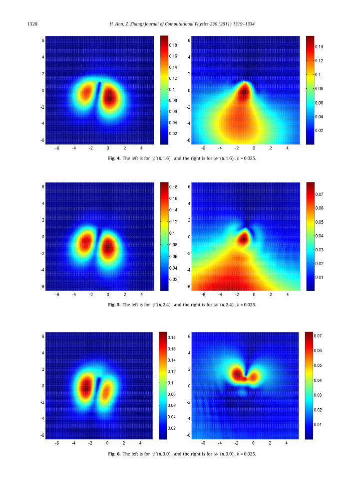
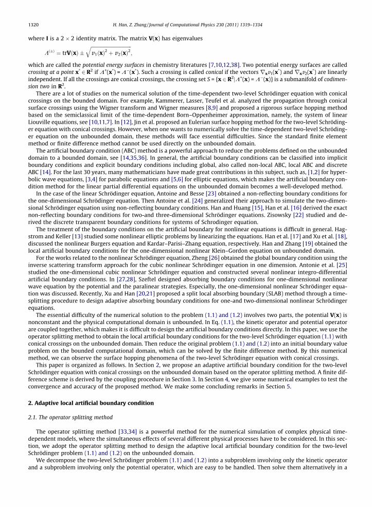
Fig. 4. The left is for j/+(x,1.6)j, and the right is for j/�(x,1.6)j, h = 0.025.
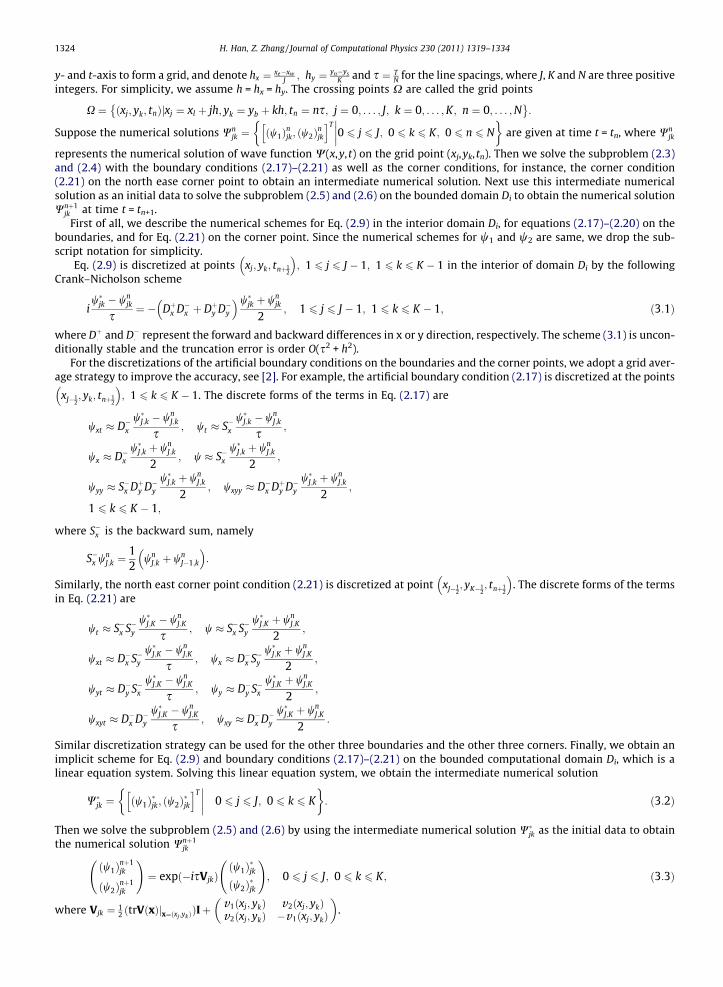
Fig. 5. The left is for j/+(x,2.4)j, and the right is for j/�(x,2.4)j, h = 0.025.
Fig. 6. The left is for j/+(x,3.0)j, and the right is for j/�(x,3.0)j, h = 0.025.
1328 H. Han, Z. Zhang / Journal of Computational Physics 230 (2011) 1319–1334
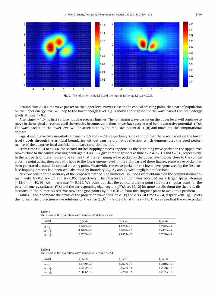
Fig. 7. The left is for j/+(x,3.6)j, and the right is for j/�(x,3.6)j, h = 0.025.
H. Han, Z. Zhang / Journal of Computational Physics 230 (2011) 1319–1334 1329
Around time t = 0.4 the wave packet on the upper level moves close to the conical crossing point, then part of populationon the upper energy level will hop to the lower energy level. Fig. 3 shows the snapshot of the wave packets on both energylevels at time t = 0.8.
After time t = 1.0 the first surface hopping process finishes. The remaining wave packet on the upper level will continue tomove in the original direction, until the velocity becomes zero, then moves back accelerated by the attractive potential K+(x).The wave packet on the lower level will be accelerated by the repulsive potential K�(x) and move out the computationaldomain.
Figs. 4 and 5 give two snapshots at time t = 1.6 and t = 2.4, respectively. One can find that the wave packet on the lowerlevel travels through the artificial boundaries without causing dramatic reflection, which demonstrates the good perfor-mance of the adaptive local artificial boundary condition method.
From time t = 2.4 to t = 3.6, the second surface hopping process happens, as the remaining wave packet on the upper levelmoves close to the conical crossing point again. Figs. 5–7 give three snapshots at time t = 2.4, t = 3.0 and t = 3.6, respectively.In the left parts of these figures, one can see that the remaining wave packet on the upper level moves close to the conicalcrossing point again, then part of it hops to the lower energy level. In the right parts of these figures, some wave packet hasbeen generated around the conical crossing point. Meanwhile, the wave packet on the lower level generated by the first sur-face hopping process had been well absorbed by boundary Rw, Rn and Rs with negligible reflections.
Next we consider the accuracy of the proposed method. The numerical solutions were obtained on the computational do-main with h = 0.2, h = 0.1 and h = 0.05, respectively. The reference solution was obtained on a larger spatial domain[�12,6] � [�10,10] with mesh size h = 0.025. We point out that the conical crossing point (0,0) is a singular point for thepotential energy surfaces K±(x) and the corresponding eigenvectors v±(x), see [9,12] for more details about the theoretic dis-cussions. In the numerical test, we move the grid points by h* = 0.0125 from this singular point to avoid this problem.
Tables 1 and 2 compare the errors of the projection wave solution /+(x) and /�(x) at time t = 2.4, respectively. Fig. 8 plotsthe norm of the projection wave solutions on the slice {(x,h*)j � 8 6 x 6 6} at time t = 1.0. One can see that the wave packet
Table 1The errors of the projection wave solution /+ at time t = 2.4.
Mesh Eþ1ð2:4Þ Eþ1 ð2:4Þ Eþ2 ð2:4Þ
h ¼ 15
9.9485e�3 1.1778e�1 1.7889e�2
h ¼ 110
4.2899e�3 5.2070e�2 7.4126e�2
h ¼ 120
1.9763e�3 2.9853e�2 3.7692e�2
Table 2The errors of the projection wave solution /� at time t = 2.4.
Mesh E�1ð2:4Þ E�1 ð2:4Þ E�2 ð2:4Þ
h ¼ 15
1.3739e�2 4.2027e�1 6.4404e�2
h ¼ 110
5.9282e�3 9.6527e�2 1.2821e�2
h ¼ 120
2.8806e�3 3.2750e�2 4.2872e�3

−8 −6 −4 −2 0 2 4 60
0.05
0.1
0.15
0.2
0.25
0.3
0.35
0.4
x
|φ+ (
x,h*
,1.0
)|h=0.2h=0.1h=0.05reference solution
−8 −6 −4 −2 0 2 4 60
0.05
0.1
0.15
0.2
0.25
0.3
0.35
0.4
x
|φ− (
x,h*
,1.0
)|
h=0.2h=0.1h=0.05reference solution
Fig. 8. Snapshots of the projection wave solutions at time t = 1.0. The left is for j/+(x,h*,1.0)j, and the right is for j/�(x,h*,1.0)j. h* = 0.0125.
−8 −6 −4 −2 0 2 4 60
0.02
0.04
0.06
0.08
0.1
0.12
x x
h=0.2h=0.1h=0.05reference solution
−8 −6 −4 −2 0 2 4 60
0.01
0.02
0.03
0.04
0.05
0.06
0.07
0.08
0.09
0.1h=0.2h=0.1h=0.05reference solution
|φ+ (
x,h*
,2.8
)|
|φ− (
x,h*
,2.8
)|
Fig. 9. Snapshots of the projection wave solutions at time t = 2.8. The left is for j/+(x,h*,2.8)j, and the right is for j/�(x,h*,2.8)j. h* = 0.0125.
−8 −6 −4 −2 0 2 4 60
0.002
0.004
0.006
0.008
0.01
0.012
0.014
0.016
x
Erro
r
h=0.2h=0.1h=0.05
h=0.2h=0.1h=0.05
−8 −6 −4 −2 0 2 4 60
0.002
0.004
0.006
0.008
0.01
0.012
0.014
0.016
x
Erro
r
Fig. 10. The errors of the projection wave solutions at time t = 2.8. The left is for /þnumðx;h�;2:8Þ � /þexaðx;h
�;2:8Þ
�� ��, and the right is for/�numðx;h
�;2:8Þ � /�exaðx; h
�;2:8Þ
�� ��. h* = 0.0125.
1330 H. Han, Z. Zhang / Journal of Computational Physics 230 (2011) 1319–1334

H. Han, Z. Zhang / Journal of Computational Physics 230 (2011) 1319–1334 1331
on the upper energy level hops to the lower energy level during the first hopping process. Fig. 9 plots the norm of the pro-jection wave solutions on the same slice at time t = 2.8, which shows that the wave packet on the upper energy level hops tothe lower energy level again during the second hopping process. Fig. 10 gives the corresponding numerical errors on thesame slice at time t = 2.8. On one hand, the numerical errors decrease fast when we refine the mesh size h. On the other hand,the numerical errors near the point (0,h*) do not decrease dramatically, which is caused by the singularity of the solutionscaused by the conical crossing point.
Fig. 11 shows the time evolution of the L1 error function between the numerical solutions and the reference solution,which illustrate the accuracy of the proposed method.
Fig. 12 plots the upper energy level population p+(t) versus time, which provides the information of the whole surfacehopping process. From time t = 0.2 to t = 1.2, the first hopping process happens. After time t = 1.2, the wave packet on theupper level moves in the original directions and the velocity will decrease, until the velocity becomes zero. Then it will turnback and accelerate toward the conical crossing point again. The second hopping process takes place between t = 2.5 and
0 0.5 1 1.5 2 2.5 3 3.5 40
0.1
0.2
0.3
0.4
0.5
0.6
t
Erro
r
0 0.5 1 1.5 2 2.5 3 3.5 40
0.1
0.2
0.3
0.4
0.5
0.6
t
Erro
r
h=0.2
h=0.1
h=0.05
h=0.2h=0.1h=0.05
Fig. 11. Time evolution of the L1 absolute error between the numerical solutions and the reference solution. The left is for Eþ1 ðtÞ, and the right is for E�1 ðtÞ.
0 0.5 1 1.5 2 2.5 3 3.5 40
0.1
0.2
0.3
0.4
0.5
0.6
0.7
0.8
0.9
1
t
Upp
er le
vel p
opul
atio
n
h=0.2h=0.1h=0.05reference solutionThe 1st hopping
The 2nd hopping
Fig. 12. The upper energy level population p+(t) versus time.

1332 H. Han, Z. Zhang / Journal of Computational Physics 230 (2011) 1319–1334
t = 3.8. Since the total population on the upper and lower energy levels will be conserved, namely, p+(t) + p�(t) = 1, "t, thepopulation on the lower energy level can be obtained from p+(t) correspondingly. Thanks to the adaptive local artificialboundary conditions, one can observe the surface hopping phenomena twice on a small domain.
Remark 2. In our previous work [12], in order to test the long time performance of the surface hopping method, for exampleto observe the second hopping process, one needs a large domain. Thanks to the artificial boundary condition, one canobserve the second hopping process in a small domain, which demonstrates the efficiency of our proposed method.
Remark 3. The proposed artificial boundary conditions are valid under the assumption that during the whole surface hop-ping process only the waves in the interior domain will move out of the domain through the artificial boundaries and therewill be no waves traveling from the exterior domain into the interior domain.
For the potential energy surfaces of the potentials Viso, all these assumptions are satisfied and the proposed artificialboundary conditions have very good performance. There are many other complicated and interesting potentials in thequantum chemistry community. For instance, the linear E e Jahn–Teller potential is given by:
VJTðxÞ ¼ bjxj2Iþ cx yy �x
� �; x ¼ ðx; yÞ 2 R2;
which models the displacement of triatomic molecules from the equilateral triangle configuration, see [37]. Here b and c arephysical constants. For the potential energy surfaces of the potentials VJT(x), our assumptions may not be satisfied. Its arti-ficial boundary conditions are complicated and will be studied in our future work.
5. Conclusion
In this paper, we present an efficient approach to obtain the artificial boundary conditions for the two-level Schrödingerequation with conical crossings on the unbounded domain. We use the windowed Fourier transform to obtain the local wavenumber information in the vicinity of artificial boundaries, and adopt the operator splitting method to obtain an adaptivelocal artificial boundary condition on the bounded computational domain. Then reduce the original problem into an initialboundary value problem, which can be solved by the finite difference method. By this numerical method, we observe thesurface hopping phenomena and study the validity and numerical accuracy of the proposed scheme.
The proposed artificial boundary conditions are valid under the conditions that during the whole surface hopping processonly the waves in the interior domain will move out of the domain through the artificial boundaries and there will be nowaves traveling from the exterior domain into the interior domain. For general cases, where both the out-going and in-goingwaves travel through the artificial boundaries, the artificial boundary conditions are complicated and will be studied in ourfuture work.
Acknowledgment
This work is supported by the National Natural Science Foundation of China (Grant No. 10971116).
Appendix A. The weighted wave number parameter selection approach
In Section 2.2, we proposed an adaptive local artificial boundary condition for the two-level Schrödinger equation on theunbounded domain based on the Padé approximation to the dispersion relation (2.11). The choice of the parameter n0 and g0
are essential to Padé approximation of the dispersion relation (2.11). Therefore, in this section we give a brief introductionabout the weighted wave number parameter selection approach, see [21] for more details. First of all, we consider the onedimensional linear Schrödinger equation
i@w@tðx; tÞ ¼ � @
2w@x2 ðx; tÞ þ VðxÞwðx; tÞ; x 2 R; t > 0; ðA:1Þ
wðx; tÞjt¼0 ¼ w0ðxÞ: ðA:2Þ
Note that for any fixed time t, the wave function w(x, t) can be expressed in terms of a Fourier series and each Fourier mode isessentially a plane wave in the space–time domain. Based on this observation, Han et al. proposed an adaptive strategy,namely, at any time t, first expand the wave function w(x, t) into Fourier series and then take one of the positive componentsso that its Fourier mode is dominant. The Fourier transform presents the frequency information of the wave function w(x, t)over the whole interior domain. However, in the issue of designing local artificial boundary conditions on the bounded do-main [xw,xe], one only cares about the frequency information of the wave function in the vicinity of the artificial boundary. Inorder to obtain the local structure of the wave in the frequency domain, they replace the Fourier transform with the windowedFourier transform.
H. Han, Z. Zhang / Journal of Computational Physics 230 (2011) 1319–1334 1333
For fixed time t, the windowed Fourier transform of the wave function w(x, t) is defined as
Wðn; tÞ ¼Z xe
xw
WðxÞwðx; tÞe�inxdx ¼Z xe
xe�LWðxÞwðx; tÞe�inxdx; ðA:3Þ
where the window function W(x) is defined by:
WðxÞ ¼1; x 2 ðxe � L; xe�;0; x 2 ½xw; xw � L�
�
and L is the window length. In [21], the authors suggest that L ¼ xe�xw4 is a good choice. One reasonable choice for the wave
number n0 = n0(t) is take the mode such that its spectrum is the maximum, namely
jWðn0; tÞj ¼ supnP0jWðn; tÞj: ðA:4Þ
The formula (A.4) is not the best choice in many practical computations. On one hand, comparison the magnitudes of all theFourier modes is not very efficient in calculations. On the other hand, when two Fourier modes are both dominant, it is obvi-ous to choose a medial value of these two different wave numbers instead of taking one of them, in order to minimize thereflection. In [21], Han et al. proposed the weighted wave number parameter selection approach, namely
n0ðtÞ ¼R1
0 njWðn; tÞjp dnR10 jWðn; tÞj
p dn; ðA:5Þ
where p is a positive real number. In [21], the authors suggest that p = 4 is a good choice. The wave number n0(t) obtainedfrom (A.5) is a weighted average of all the wave number information, therefore it is more robust and accurate.
Extension of the adaptive parameter selection for one-dimensional version to multi-dimensional cases is straightforward.Since a multi-dimensional problem can be split into a series of one-dimensional ones, one can obtain the estimation of theparameters at every boundary grid points by a dimension-by-dimension procedure. For example, for any fixed time t, in or-der to compute the wave number n0(y, t) on the east boundary Re, we use the windowed Fourier transform in x direction:
W1ðn; y; tÞ ¼Z xe
xe�LðyÞw1ðx; y; tÞe�inxdx; ðA:6Þ
where the window length is a function of y. The parameter n0(y, t) can be determined by
n0ðy; tÞ ¼R1
0 njW1ðn; y; tÞjp dnR10 jW1ðn; y; tÞjp dn
: ðA:7Þ
The parameters on other artificial boundaries can be obtained similarly.
References
[1] B. Engquist, A. Majda, Absorbing boundary conditions for the numerical simulation of waves, Math. Comput. 31 (1977) 629–651.[2] R.L. Higdon, Absorbing boundary conditions for difference approximations to the multi-dimensional wave equation, Math. Comput. 47 (1986) 437–
459.[3] L. Halpern, J. Rauch, Absorbing boundary conditions for diffusion equations, Numer. Math. 71 (1995) 185–224.[4] H. Han, Z. Huang, Exact and approximating boundary conditions for the parabolic problems on unbounded domains, Comput. Math. Appl. 44 (2002)
655–666.[5] H.D. Han, X.N. Wu, Approximation of infinite boundary condition and its applications to finite element methods, J. Comput. Math. 3 (1985) 179–192.[6] D.H. Yu, Approximation of boundary conditions at infinity for a harmonic equation, J. Comput. Math. 3 (1985) 219–227.[7] G.A. Worth, L.S. Cederbaum, Beyond Born–Oppenheimer: molecular dynamics through a conical intersection, Ann. Rev. Phys. Chem. 55 (2004) 127–
158.[8] C. Lasser, S. Teufel, Propagation through conical crossings: an asymptotic semigroup, Commun. Pure Appl. Math. 58 (2005) 1188–1230.[9] C.F. Kammerer, C. Lasser, Wigner measures and codimension two crossings, J. Math. Phys. 44 (2) (2003) 507–527.
[10] S. Kube, C. Lasser, M. Weber, Monte Carlo sampling of Wigner functions and surface hopping quantum dynamics, J. Comput. Phys. 228 (2009) 1947–1962.
[11] C. Lasser, T. Swart, S. Teufel, Construction and validation of a rigorous surface hopping algorithm for conical crossings, Commun. Math. Sci. 5 (4) (2007)789–814.
[12] S. Jin, P. Qi, Z.W. Zhang, An Eulerian surface hopping method for the Schrödinger equation with conical crossings, SIAM Multiscale Model. Simul.submitted for publication.
[13] T. Hagstrom, H.B. Keller, Asymptotic boundary conditions and numerical methods for nonlinear elliptic problems on unbounded domains, Math.Comput. 48 (1987) 449–470.
[14] H. Han, The Artificial Boundary Method-Numerical Solutions of Partial Differential Equations on Unbounded Domains, Frontier and Prospects ofContemporary Applied Mathematics, Higher Education Press, World Scientific, 2005.
[15] H. Han, Z. Huang, Exact artificial boundary conditions for the Schrödinger equations in R2, Commun. Math. Sci. 2 (2004) 79–94.[16] H. Han, D. Yin, Z. Huang, Numerical solutions of Schrödinger equations in R3, Numer. Methods Partial Differ. Equ. 23 (2007) 511–533.[17] H.D. Han, X.N. Wu, Z.L. Xu, Artificial boundary method for Burgers’ equation using nonlinear boundary conditions, J. Comput. Math. 24 (2006) 295–304.[18] Z. Xu, H. Han, X. Wu, Numerical method for the deterministic Kardar–Parisi–Zhang equation in unbounded domains, Commun. Comput. Phys. 1 (2006)
481–495.[19] H. Han, Z.W. Zhang, Split local absorbing conditions for one-dimensional nonlinear Klein–Gordon equation on unbounded domain, J. Comput. Phys.
227 (2008) 8992–9004.[20] Z. Xu, H. Han, Absorbing boundary conditions for nonlinear Schrödinger equations, Phys. Rev. E 74 (2006) 037704.

1334 H. Han, Z. Zhang / Journal of Computational Physics 230 (2011) 1319–1334
[21] Z. Xu, H. Han, X. Wu, Adaptive absorbing boundary conditions for Schrödinger-type equations: application to nonlinear and multi-dimensionalproblems, J. Comput. Phys. 225 (2007) 1577–1589.
[22] A. Zisowsky, Discrete Transparent Boundary Conditions for Systems of Evolution Equations, Ph.D. Thesis, Technische Universitat Berlin, July 2003.[23] X. Antoine, C. Besse, Unconditionally stable discretization schemes of non-reflecting boundary conditions for the one-dimensional Schrödinger
equation, J. Comput. Phys. 188 (2003) 157–175.[24] X. Antoine, C. Besse, V. Mouysset, Numerical Schemes for the simulation of the two-dimensional Schrödinger equation using non-reflecting boundary
conditions, Math. Comput. 73 (248) (2004) 1779–1799.[25] X. Antoine, C. Besse, S. Descombes, Artificial boundary conditions for one-dimensional cubic nonlinear Schrödinger equations, SIAM J. Numer. Anal. 43
(2006) 2272–2293.[26] C. Zheng, Exact nonreflecting boundary conditions for one-dimensional cubic nonlinear Schrödinger equations, J. Comput. Phys. 215 (2006) 552–565.[27] J. Szeftel, Absorbing boundary conditions for nonlinear scalar partial differential equations, Comput. Methods Appl. Mech. Eng. 195 (2006) 3760–3775.[28] J. Szeftel, Absorbing boundary conditions for one-dimensional nonlinear Schrödinger equations, Numer. Math. 104 (2006) 103–127.[29] B. Engquist, A. Majda, Absorbing boundary conditions for the numerical simulation of waves, Math. Comput. 31 (1977) 629–651.[30] T. Shibata, Absorbing boundary conditions for the finite-difference time-domain calculation of the one dimensional Schrödinger equation, Phys. Rev. B
43 (1991) 6760.[31] J.-P. Kuska, Absorbing boundary conditions for the Schrödinger equation on finite intervals, Phys. Rev. B 46 (1992) 5000.[32] T. Fevens, H. Jiang, Absorbing boundary conditions for the Schrödinger equation, SIAM J. Sci. Comput. 21 (1999) 255–282.[33] S. Yu, S. Zhao, G.W. Wei, Local spectral time splitting method for first-and second-order partial differential equations, J. Comput. Phys. 206 (2005) 727–
780.[34] G. Strang, On the construction and comparison of difference schemes, SIAM J. Numer. Anal. 5 (1968) 506–517.[35] S.V. Tsynkov, Numerical solution of problems on unbounded domains: a review, Appl. Numer. Math. 27 (1998) 465–532.[36] H. Han, X. Wu, Artificial Boundary Condition Methods, vol. 27, Tsinghua Press, Beijing, 1998 (in Chinese).[37] G. Worth, L. Cederbaum, Beyond Born–Oppenheimer: molecular dynamics through a conical intersection, Ann. Rev. Phys. Chem. 55 (2004) 127–158.[38] G. Hagedorn, Molecular Propagation Through Electron Energy Level Crossings, Memories of the American Mathematical Society, vol. 111, AMS,
Providence, RI, 1994.