Journal of Computational Physics 356 (2018) 261–281

Contents lists available at ScienceDirect

Journal of Computational Physics

www.elsevier.com/locate/jcp

A boundary element method for Stokes flows with interfaces

Edoardo Alinovi ∗, Alessandro Bottaro

DICCA, Scuola Politecnica University of Genova, 1 via Montallegro, 16145 Genova, Italy

a r t i c l e i n f o a b s t r a c t

Article history:Received 1 April 2017Received in revised form 6 October 2017Accepted 4 December 2017Available online 7 December 2017

Keywords:Boundary element methodEnforcement of mass conservationSuperhydrophobic surfaces

The boundary element method is a widely used and powerful technique to numerically describe multiphase flows with interfaces, satisfying Stokes’ approximation. However, low viscosity ratios between immiscible fluids in contact at an interface and large surface tensions may lead to consistency issues as far as mass conservation is concerned. A simple and effective approach is described to ensure mass conservation at all viscosity ratios and capillary numbers within a standard boundary element framework. Benchmark cases are initially considered demonstrating the efficacy of the proposed technique in satisfying mass conservation, comparing with approaches and other solutions present in the literature. The methodology developed is finally applied to the problem of slippage over superhydrophobic surfaces.

© 2017 Elsevier Inc. All rights reserved.

1. Introduction

Multiphase flows are ubiquitous in Nature and their prediction is of great importance in scientific and engineering applications. Over the last few decades, many computational methods have been developed to numerically investigate this important class of complex flows. Among these, the boundary integral methods (BIM) assumes a considerable relevance from both a theoretical and a numerical point of view, particularly when the Stokes’ approximation is applicable. In the Stokes flow regime, the Reynolds number is negligible and the governing equations become linear, allowing the reconstruction of the total flow field by appropriate point sources and dipoles distribution at the boundaries of the fluid domain. The method has found noteworthy success in the simulation of emulsions [1,2] and droplet interactions [3–5], both in free space and bounded domains. The main advantage of this method is that the flow equations are solved only for the unknown stress and velocity fields at the domain boundaries and at fluid interfaces, rather than in the bulk flow. The numerical counterpart of BIM is the boundary element method (BEM), which, in practice, recasts the integral equations in discrete form for a set of elements of fixed shape, approximating the boundary of the domain/fluid interfaces. The BEM is thus a mesh-less method and this feature renders it suitable to study complex geometries and moving interfaces, without any additional complication related to mesh quality or mesh deformation. In this paper, attention is focused on the problem of mass conservation inside closed volumes of fluid creating an interface with an outer fluid. Calling λ the viscosity ratio between the inner and the outer fluid, mass leakage may occur when λ < 1, with increasing magnitude as the viscosity ratio decreases. This phenomenon has already been pointed out by Pozrikidis [6], who also offered a correction, which involves a slight modification of the governing integral equations. Here, we propose an alternative method based on constraining the interfacial velocity to respect the continuity equation. The procedure is applicable to any type of boundary element code and

* Corresponding author.E-mail address: edoardo.alinovi@dicca.unige.it (E. Alinovi).

https://doi.org/10.1016/j.jcp.2017.12.0040021-9991/© 2017 Elsevier Inc. All rights reserved.

262 E. Alinovi, A. Bottaro / Journal of Computational Physics 356 (2018) 261–281

Fig. 1. Sketch of two different fluid domains separated by the interface I. The letters T, L, R, I and W denote, respectively, the top, left, right boundaries, the interface and the wall. In the figure, L and R boundaries are periodic and W comprises all the walls of the cavity.

involves simple modifications with respect to the standard algorithm. In the following we will first present the mathematical formulation of the problem, describing the boundary integral equations arising from the analysis of two-phase Stokes flows and their numerical treatment into a boundary element framework. We then present the results of the calculations of selected benchmark cases. As final example, we use the numerical method developed to approach the problem of the slippage over superhydrophobic surfaces, calculating protrusion heights (or Navier slip lengths), taking into account the viscosity ratio and the deformation of the interface.

2. Mathematical formulation

We consider problems involving creeping flow in a region with different domains filled with immiscible, incompressible fluids. The well-known governing equations for this type of problems read

μ∇2u = ∇p, ∇ · u = 0, (1)

where u is the fluid velocity, p is the pressure and μ is the dynamic viscosity in each given domain.We use the boundary integral method to transform the differential problem into an integral one to be solved by the

boundary element technique. Even if we derive the boundary integral formulation for a particular domain, sketched in Fig. 1, the same procedure applies to different shapes of the boundary, leading to formally similar integral equations.

We start by considering a two-dimensional domain filled with two viscous fluids of viscosity ratio λ = μ1

μ2; fluid 1 is

found in domain �1, while fluid 2 is contained within �2. The position of the interface, I, of unit normal n when seen from �1, must be found from the conservation equations. The basic idea underlying the boundary integral method is that a Stokes velocity field in a generic domain � may be reconstructed using only values of the velocity and stress fields on the closed boundary C of the domain; this can be done by introducing two integral operators. One is called the single-layer-potential and employs a function G i j(x, x0) which represents the velocity field generated by a single point force at x; integrating with respect to the arclength around C the product of G i j times the surface force of strength f i(x) yields the velocity field generated by the distribution of surface forces. The second integral, the double-layer-potential, is interpreted as a linear distribution in C of sources (or sinks) of strength u · n plus a symmetric placement of point forces (i.e. dipoles). The single-and the double-layer potentials for Stokes flow in two dimensions are:

F S L Pj (x0, f ;C) = 1

4πμ

∫C

f i(x)G i j(x, x0)dl(x), (2)

F DL Pj (x0, u;C) = 1

4π

∫C

ui(x)T i jk(x, x0)nk(x)dl(x), (3)

where:

• G i j is the velocity Green’s function for the two-dimensional Stokes flow, eventually satisfying specific boundary condi-tions for convenience;

• T i jk is the stress tensor associated to G i j ;• x and x0 are, respectively, the so-called field point and the integral point in the interior of the domain �;

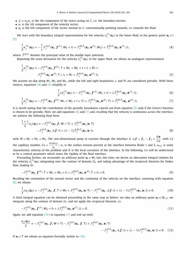
E. Alinovi, A. Bottaro / Journal of Computational Physics 356 (2018) 261–281 263

• f i = σi jn j is the ith component of the stress acting on C , i.e. the boundary traction;• ui is the ith component of the velocity vector;• nk is the kth component of the vector normal to C , conventionally pointing inwards, i.e. towards the fluid.

We start with the boundary integral representation for the velocity u(1)j (x0) in the lower fluid, in the generic point x0 ∈ I

[7]

1

2u(1)

j (x0) = −1

λF S L P

j (x0, f (1);W3 + I) +F DL Pj (x0, u(1);W3) + F DL P

j (x0, u(1); I), (4)

where F DL P denotes the principal value of the double layer potential.Repeating the same derivation for the velocity u(2)

j (x0) in the upper fluid, we obtain an analogous representation

1

2u(2)

j (x0) = −F S L Pj (x0, f (2);T + W1 + W2 + I + L + R) +

F DL Pj (x0, u(2);T + L + R) + F DL P

j (x0, u(2); I). (5)

We assume no-slip along W1, W2 and W3, while the left and right boundaries, L and R, are considered periodic. With these choices, equations (4) and (5) simplify in

1

2λu(1)

j (x0) = −F S L Pj (x0, f (1);W3 + I) + λF DL P

j (x0, u(1); I), (6)

1

2u(2)

j (x0) = −F S L Pj (x0, f (2);W1 + W2 + I + T) +F DL P

j (x0, u(2);T) + F DL Pj (x0, u(2); I). (7)

It is worth noting that the contribution of the periodic boundaries cancels out from equation (5) only if the Green’s function is chosen to be periodic. Next, we add equations (6) and (7) and, recalling that the velocity is continuous across the interface, we achieve the following final form:

1 + λ

2u j(x0) = −F S L P

j (x0, f ;W + T) +F DL Pj (x0, u;T)

−F S L Pj (x0,� f ; I) + (λ − 1)F DL P

j (x0, u; I), (8)

with W = W1 + W2 + W3. The non-dimensional jump in traction through the interface is � f = f 1 − f 2 = K n

Ca, with Ca

the capillary number, Ca = μ2uref

σs; σs is the surface tension present at the interface between fluids 1 and 2, uref is some

characteristic velocity of the problem and K is the local curvature of the interface. In the following, Ca will be understood to be a control parameter which tunes the rigidity of the fluid interface.

Proceeding further, we reconsider an arbitrary point x0 ∈ W3 but, this time, we derive an alternative integral relation for the velocity u(1)

j (x0) integrating over the contour of domain �2 and taking advantage of the reciprocal theorem for Stokes flow, leading to:

−F S L Pj (x0, f (2);T + W1 + W2 + I) +F DL P

j (x0, u(2);T + I) = 0. (9)

Recalling the orientation of the normal vector and the continuity of the velocity on the interface, summing with equation (6) we obtain:

1

2λu j(x0) = −F S L P

j (x0, f ;T + W) +F DL Pj (x0, u;T) −F S L P

j (x0,� f ; I) + (λ − 1)F DL Pj (x0, u; I) = 0. (10)

A third integral equation can be obtained proceeding in the same way as before: we take an arbitrary point x0 ∈ W1,2, we integrate along the contour of domain �1 and we apply the reciprocal theorem, i.e.

−F S L Pj (x0, f (1);W3 + I) + λF DL P

j (x0, u(1); I) = 0. (11)

Again, we add equation (11) to equation (7) and end up with:

u j(x0)

2= −F S L P

j (x0, f ;W + T) −F S L Pj (x0, f ;T) +F DL P

j (x0, u;T)

−F S L Pj (x0,� f ; I) + (λ − 1)F DL P

j (x0, u; I) = 0. (12)

If x0 ∈ T we obtain an equation formally similar to (12)

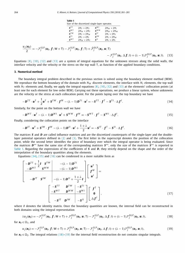
264 E. Alinovi, A. Bottaro / Journal of Computational Physics 356 (2018) 261–281

Table 1Size of the discretized single-layer operator.

S T T 2NT × 2NT S W I 2NW × 2NI

S W T 2NW × 2NT S W W 2NW × 2NW

S T W 2NT × 2NW S I T 2NI × 2NT

S T I 2NT × 2NI S I W 2NI × 2NW

S W T 2NW × 2NT S I I 2NI × 2NI

u j(x0)

2= −F S L P

j (x0, f ;W + T) −F S L Pj (x0, f ;T) + F DL P

j (x0, u;T)

−F S L Pj (x0,� f ; I) + (λ − 1)F DL P

j (x0, u; I). (13)

Equations (8), (10), (12) and (13) are a system of integral equations for the unknown stresses along the solid walls, the interface velocity and the velocity or the stress on the top wall T, as function of the applied boundary conditions.

3. Numerical method

The boundary integral problem described in the previous section is solved using the boundary element method (BEM). We reproduce the bottom boundary of the domain with NW discrete elements, the interface with NI elements, the top wall with NT elements and, finally, we apply the integral equations (8), (10), (12) and (13) at the elements’ collocation points (at least one for each element for low order BEM). Carrying out these operations, we produce a linear system, whose unknowns are the velocity or the stress at each collocation point. For the points laying over the top boundary we have

−DT T · uT + 1

2uT + S T W · f W − (λ − 1)DT I · u I = −S T T · f T − S T I · � f I . (14)

Similarly, for the point on the bottom wall we have

−DW T · uT − (λ − 1)DW I · u I + S W W · f W = −S W T · f T − S W I · � f I . (15)

Finally, considering the collocation points on the interface

−D I T · uT + S I W · f W − (λ − 1)D I I · u I + 1 + λ

2u I = −S I T · f T − S I I · � f I . (16)

The matrices S and D are called influence matrices and are the discretized counterparts of the single-layer and the double-layer potential operators defined in (2) and (3). The first letter in the superscript denotes the position of the collocation point, while the second letter identifies the piece of boundary over which the integral operator is being evaluated. Since the matrices D∗∗ have the same size of the corresponding matrices S∗∗ , only the size of the matrices S∗∗ is reported in Table 1. Regarding the expressions of the coefficients of S and D , they strictly depend on the shape and the order of the interpolation of the boundary quantities along the elements.

Equations (14), (15) and (16) can be condensed in a more suitable form as⎡⎢⎢⎢⎢⎢⎣

−DT T + 1

2I S T W −(λ − 1)DT I

−DW T S W W −(λ − 1)DW I

−D I T S I W −(λ − 1)D I I + 1 + λ

2I

⎤⎥⎥⎥⎥⎥⎦

⎡⎢⎣

uT

f W

u I

⎤⎥⎦ =

⎡⎢⎢⎢⎣

−S T T DT W −S T I

−S W T DW W −S W I

−S I T D I W −S I I

⎤⎥⎥⎥⎦

⎡⎢⎣

f T

0

� f I

⎤⎥⎦ , (17)

where I denotes the identity matrix. Once the boundary quantities are known, the internal field can be reconstructed in both domains using the integral representation

λu j(x0) = −F S L Pj (x0, f ;W + T) +F DL P

j (x0, u;T) −F S L Pj (x0,� f ; I) + (λ − 1)F DL P

j (x0, u; I), (18)

for x0 ∈ �1, and

u j(x0) = −F S L Pj (x0, f ;W + T) +F DL P

j (x0, u;T) −F S L Pj (x0,� f ; I) + (λ − 1)F DL P

j (x0, u; I), (19)

for x0 ∈ �2. The integral relations (18)–(19) for the internal field reconstruction do not contains singular integrals.

E. Alinovi, A. Bottaro / Journal of Computational Physics 356 (2018) 261–281 265

In our implementation, all the boundaries are approximated by cubic spline segments, while we assume a linear vari-ation of the boundary quantities along each element. The advantages of the cubic splines are the high fidelity in fitting complex boundaries and the possibility of computing the curvature at the collocation points directly from the polynomial representation of the target element. We employ discontinuous elements at boundaries’ sharp corners to deal with the sin-gularity of the stress f , which often arises [7]. In this particular case, the collocation points are placed in specified locations along the segments, obtained from the roots of the first order Radau’s polynomial. For all the other elements, the collocation points are located at the extremities of the segment; in this case, since a collocation point is shared between two adjacent elements, the boundary quantities are approximated in a continuous way. The six points Gauss–Legendre quadrature for-mula is employed for the numerical evaluation of the non-singular integrals arising from the boundary element formulation. The weakly singular integral case, due to the structure of the Green’s function for the Stokes flow, which usually involves natural logarithms in the two dimensional case, is treated subtracting off the singularity from the integrand function and using basic analytical techniques for the successive integration. The collocation points along the interface are advanced in time using the following rule

dx(i)

dt= (ui · ni)ni, i = 1, . . . , NI , (20)

where x(i) are the ith collocation point and ni is normal to the interface at x(i) . Using the normal velocity to advance the interface, instead of the velocity u, is found to be very effective in limiting the spreading of the collocation points, with the consequent advantage that the interface does not need to be frequently remeshed. Equation (20) can be discretized with any explicit scheme for ordinary differential equations. We have implemented both the first order Euler and the second order Runge–Kutta (RK2) integration, finding very few differences between the two schemes. However, since the RK2 scheme requires the evaluation of the interfacial velocity at two different time steps, with the consequent solution of the boundary element system, we prefer a simpler and faster one-step integration.

A detailed review of the boundary element method for Stokes flows is given in [8]. Details of the current implementation can be found in Appendix A.

3.1. Enforcement of mass conservation

One hidden issue in solving flows in the presence of interfaces, is that a unique solution of the integral equations cannot be found for arbitrary values of the viscosity ratio λ. This was described in particular by Pozrikidis [7,8], and the drawback encountered in solving such equations is that a leak or an increase of the mass of fluid inside a closed domain may occur in time; this phenomenon becomes more important as the viscosity ratio λ decreases [9]. One way to deal with this problem and remove the non-uniqueness of the solution is proposed in [6] and requires adding the following term

z j(x0)

∫C

ui(x)ni(x)dl (21)

to the double-layer potential along the interface into the integral equations. Here z j(x0) is an arbitrary function such that ∫C

zini �= 0, with n j the normal vector to the interface. The simplest choice is z j = n j and, since this term shifts the eigen-

values of the double-layer potential operator, the procedure is known as deflation.An alternative method to ensure mass conservation is proposed here. We start by noting that each boundary integral

problem can be reduced to the solution of a linear system of the type:

Ax = b, (22)

where A and b are the boundary element matrix and the right-hand-side, dependent on the original boundary integral formulation of the problem, while x is the vector containing the unknowns (cf. equation (17)). For incompressible flows, the mass conservation inside a domain �i can be readily written as

∇ · u = 0, (23)

with u the velocity vector inside the domain �i . Integrating (23) over the volume �i and taking advantage of Green’s theorem we obtain∫

∂�

u · n dS = 0. (24)

The integral relation (24) can be discretized in the same fashion as the single-layer and the double-layer potentials, leading to a simple linear equation of the form

266 E. Alinovi, A. Bottaro / Journal of Computational Physics 356 (2018) 261–281

c · u = 0, (25)

where c is a vector containing the coefficients of the unknown velocity at the collocation points. The form of the coefficient depends, again, on the type of collocation method chosen to discretize the boundary integral equation. If we are in the presence of multiple fluid volumes, we can easily extend expression (25) as

C x = 0. (26)

The ith row of the matrix C contains the coefficients arising from the discretization of equation (24) for the ith fluid domain. Clearly, the matrix C will present zero entries for those unknowns which are not the interfacial velocities to be constrained. We now wish to add the set of mass-conservation constraints to the boundary element system (22); this is not an easy task since, usually, the system is already closed and simply adding an additional constraint equation will lead to an over-determined system. Discharging as many equations as the number of constraints would be an available option, but it is not clear which equations are to be substituted and a loss of accuracy might result. To solve this issue, the idea is to introduce in the system each additional equation with associated an unknown Lagrange multiplier �, which will render the boundary element system well balanced and force the solution to respect mass conservation for any value of λ. We consider the following Lagrangian functional

L = 1

2xT Ax − xT b + �T (C x), (27)

where the first two terms in the L function represent the potential energy of the unconstrained system, while the last term represents the energy needed to maintain the constraints. � is a vector containing the Lagrange multipliers, one for each interface within the domain �. Now, we proceed to minimize L, requiring that its total variation, δL, is zero for every possible value of δx and δ�, thus

δL = ∂L∂x

· δx + ∂L∂�

· δ� = 0, (28)

which leads to the following conditions over the gradient of the Lagrangian functional:

∂L∂x

= 0,∂L∂�

= 0. (29)

By imposing the conditions above, we produce a new linear system, which incorporates the desired constraints:[A C T

C 0

][x�

]=

[b0

]. (30)

This method is of easy implementation and, since usually the boundary element matrix is dense, it does not destroy an eventually banded form of the final matrix. However, the size of the matrix increases and this can become undesirable when a large number of interfaces is present.

3.2. Physical interpretation of the Lagrange multiplier

In order to describe the physical meaning of the Lagrange multiplier �, we reconsider a slightly modified, but more general, version of equation (24):∫

∂�

u · n dS = q∗, (31)

which assigns a generic value to the flow rate across the target boundary. The relation (31) can be readily discretized in

C x = q, (32)

where the right hand side q takes into account possible flow of fluid through the boundary ∂�.The Lagrangian functional now takes the form:

L = 1

2xT Ax − xT b + �T (C x − q) = E(x,q) + �T (C x − q), (33)

with E(x, q) the energy associated with the boundary element linear system. Deriving the Lagrangian with respect to q we obtain:

∂L = ∂E − �T , (34)

∂q ∂q

E. Alinovi, A. Bottaro / Journal of Computational Physics 356 (2018) 261–281 267

Fig. 2. An elliptic droplet deforming into a circle. The right figure shows the evolution of the interface in time.

and stationarity implies that

∂E∂q

= �T , (35)

i.e. the Lagrange multiplier � represents the sensitivity of the energy E of the system with respect to variations in the mass flow rate through the contour ∂�.

4. Results

4.1. Relaxation of a two-dimensional droplet

We start by studying a simple benchmark case: the relaxation of a two dimensional droplet from an ellipse of given aspect ratio, as show in Fig. 2. We assume that the droplet, initially at rest, lies in an infinite free space filled with a different fluid. The droplet will start to contract, under the effect of surface tension, until a circular shape is reached. During the droplet’s contraction, the evolution of the semi-major axis a is monitored, up to the steady state.

In order to perform this study we take advantage of the free space Green’s function and its associated stress tensor, which read

Gij(x, x0) = −δi jlog(r) + xi x j

r2, Tijk(x, x0) = −4

xi x j xk

r4, (36)

where r is the distance between the points x and x0, while xi = xi − x0i .Regarding the boundary integral formulation, we note that this case corresponds to solving the system[

(λ − 1)D I I + 1 + λ

2I][

u]

= −S I I� f I , (37)

for the interfacial velocity u, with the unit normal vector pointing outside of the droplet. We can force the system to respect the mass conservation constraint following the formulation in equation (30). Since in this case we have only one interface, the matrix C degenerates to a single equation, and, in practice, only one line and one column must be added to the original linear system.

For this problem we consider three different values of the viscosity ratio, λ = 1

10,

1

20,

1

100, and three different values

of the capillary number, Ca = 0.1, 1, 10, which tunes the rigidity of the interface and the velocity of the relaxation. Since the aspect ratio of the ellipse is

a

b= 2, we aspect that, after a transient, the fluid interface assumes a circular shape with

radius equal to √

2 (provided b is initially set to one). For this simulation we use 60 spline elements and employ a fixed time step �t = 0.01 for the lower capillary number, while �t = 0.05 for the others. The number of elements is selected in order to obtain a good matching with respect to the steady state radius of the droplet (here we obtain a value close to the theoretical one, up to the fourth decimal place). However, a lower number of element would be equally satisfactory, since the spline elements are very suitable to discretize curved boundaries. The time step is selected in order to have a stable time evolution of the interface, which could in principle suffer of numerical instability due to the explicit scheme used. Its influence on the simulations is negligible since the Stokes equation is being solved under the quasi-steady approximation. For the simulations, we have developed a boundary element code with our new mass-conservation strategy embedded in the system. We have validated our implementation (without the Lagrange multiplier approach) against the code written by Pozrikidis and publicly available with the library BEMLIB [10], finding indistinguishable differences between the results of the two codes. In the following we will call this latter method the standard approach, to distinguish it from techniques – such as the new one described in this paper – which enforce continuity explicitly.

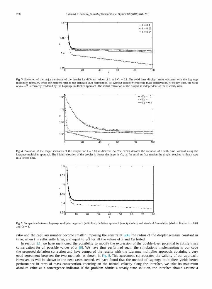
The results, reported in Fig. 3 and 4, compare the evolution of semi-major axis, a, in time for both the Lagrange multiplier approach and the standard formulation. Even if the initial transient path is similar, we note (symbols) a continuous decrease of the semi-axis a after the droplet has reached the circular shape. The effect of this mass loss is enhanced as the viscosity

268 E. Alinovi, A. Bottaro / Journal of Computational Physics 356 (2018) 261–281

Fig. 3. Evolution of the major semi-axis of the droplet for different values of λ and Ca = 0.1. The solid lines display results obtained with the Lagrange multiplier approach, while the markers refer to the standard BEM formulation, i.e. without explicitly enforcing mass conservation. At steady state, the value of a = √

2 is correctly rendered by the Lagrange multiplier approach. The initial relaxation of the droplet is independent of the viscosity ratio.

Fig. 4. Evolution of the major semi-axis of the droplet for λ = 0.01 at different Ca. The circles denotes the variation of a with time, without using the Lagrange multiplier approach. The initial relaxation of the droplet is slower the larger is Ca, i.e. for small surface tension the droplet reaches its final shape in a longer time.

Fig. 5. Comparison between Lagrange multiplier approach (solid line), deflation approach (empty circles), and standard formulation (dashed line) at λ = 0.01and Ca = 1.

ratio and the capillary number become smaller. Imposing the constraint (24), the radius of the droplet remains constant in time, when t is sufficiently large, and equal to

√2 for all the values of λ and Ca tested.

In section 3.1, we have mentioned the possibility to modify the expression of the double-layer potential to satisfy mass conservation for all possible values of λ [6]. We have thus performed again the simulations implementing in our code the proposed deflation correction and have compared the results with the Lagrange multiplier approach, obtaining a very good agreement between the two methods, as shown in Fig. 5. This agreement corroborates the validity of our approach. However, as will be shown in the next cases treated, we have found that the method of Lagrange multipliers yields better performance in term of mass conservation. Focusing on the normal velocity along the interface, we take its maximum absolute value as a convergence indicator. If the problem admits a steady state solution, the interface should assume a

E. Alinovi, A. Bottaro / Journal of Computational Physics 356 (2018) 261–281 269

Fig. 6. Maximum normal velocity history. The dashed line corresponds to the standard (unconstrained) implementation, the line with empty circles corre-spond to the deflation approach, while the solid line correspond to the Lagrange multiplier approach.

Fig. 7. Sketch of the cavity with a wavy interface (left), and successive positions assumed by the interface during its relaxation into a parabolic shape (right).

position such that the maximum normal velocity vanishes. The comparison between the methods is shown in Fig. 6. We observe that the maximum normal velocity decreases until reaching a plateau, whose value is dependent on the number of element used to discretize the droplet and goes down as the number of elements increases. The Lagrange multipliers approach offers a better performance in minimizing the maximum normal velocity along the droplet’s interface at steady state, which is several orders of magnitude lower with respect to the method proposed by Pozrikidis [6] at the same spatial resolution and time step. We have found out during the simulations that mass leakage depends on the number of elements employed, decreasing with the increase of the resolution. It is worth observing that the problem of mass conservation at low viscosity ratios is intrinsic to the boundary element method and using a large number of elements does not solve the problem at the source. The method described here is more accurate (at any given resolution) and computationally efficient.

4.2. Relaxation of a pinned interface

For this numerical example, we consider a simple cavity bounded by three walls of length L and a fluid interface, pinned at the corners of the cavity, as sketched in Fig. 7. The initial shape of the interface is a cosine wave of equation

y0(x) = b cos(2π

Lx) − b,

where b is a constant. Similarly to the droplet’s case, the surface tension between the two fluids induces the motion of the interface, which experiments a transition from the initial shape to a prescribed shape, analytically available under the hypothesis of small amplitude deflection of the interface. The Young–Laplace equation, expressed for convenience in non-dimensional form, is

d2 y2

[1 +

(dy )2]− 32 = C1, (38)

dx dx

270 E. Alinovi, A. Bottaro / Journal of Computational Physics 356 (2018) 261–281

with C1 = �P the non-dimensional pressure jump across the interface and y the vertical displacement of the interface. If the curvature of the interface is small enough, the term in brackets in equation (38) tends to one, leading to the following approximate solution

y(x) = C1

2x(x − L), (39)

after imposing the boundary conditions

y(0) = 0, y(L) = 0. (40)

Particular attention should be payed to the constant C1: since the pressure difference across the interface is not known a priori, its value can be calculated imposing the conservation of mass inside the cavity through the relation:

L∫0

y0dx =L∫

0

y f dx, (41)

which yields C1 = 12b

L2. In order to obtain more precise results, equation (38) can be solved without approximation using

standard iterative techniques.For this simulation, we have employed 60 elements to discretize each edge of the cavity and the interface. We have set

a constant time step �t = 10−3 for Ca = 0.1, while �t = 10−2 for the lower values of Ca. The fluid in both the domains is initially at rest and the interface moves as an effect of surface tension. Periodic boundary condition are applied to left and right boundaries by using the following Green’s function [8]:

A(x) = 1

2log{2[cosh(ωx2) − cos(αx1)]}, (42)

G11 = −A(x) − y∂ A(x)

∂ y+ 1, (43)

G12 = y∂ A(x)

∂ x, (44)

G22 = A(x) + y∂ A(x)

∂ x, (45)

where x = x − x0 and α = 2πL . The components of the stress tensor T i jk are:

T111 = −4∂ A(x)

∂ x− 2x2

∂2 A(x)

∂ x∂ y, T112 = −2

∂ A(x)

∂ y− 2x2

∂2 A(x)

∂ y∂ y, (46)

T212 = 2x2∂2 A(x)

∂ x∂ y, T222 = −2

∂ A(x)

∂ y+ 2x2

∂2 A(x)

∂ y∂ y, (47)

with no need to specify the missing components of G i j and T i jk since they are symmetric tensors.In this case, we monitor the volume of the fluid trapped between the cavity walls and the interface, given, at each time,

by the following integral relation

V =∫�1

dS = 1

2

∫�1

∇ · x dS = 1

2

∫∂�1

x · n dl, (48)

which is integrated in the same fashion as other integral quantities. The results, reported in Figs. 8 and 9, shown a similar behavior to that observed in the droplet relaxation benchmark. The total mass inside the cavity is not conserved in time and mass leakage becomes larger as the capillary number and the viscosity ratio become smaller. The usage of the deflation approach (21) turns out to be not as effective as in the previous case and the mass leakage (or creation) persists, even if with a lower growth rate, as shown in Fig. 10. Instead, the Lagrange multiplier approach leads to very satisfactory results, maintaining constant the mass inside the pocket and fitting the theoretical steady-state position of the interface prescribed by equation (38) for every test value of λ and Ca, as shown in Fig. 11 for a representative case.

Additional features arise from the analysis of the maximum absolute value of the normal velocity along the interface during the relaxation process, shown for a representative set of parameters in Fig. 12. We note that the standard bound-ary element formulation is unstable: the initial decrease in the maximum value of the normal velocity is followed by an increase. This phenomenon brings, sooner or later, to the divergence of the simulation, with the interface breaking down anomalously. The double-layer deflation seems to counteract this undesirable effect, but it presents some difficulties in

E. Alinovi, A. Bottaro / Journal of Computational Physics 356 (2018) 261–281 271

Fig. 8. Time variation of the volume of fluid contained inside the cavity (V 0 is the initial value) for different values of λ and Ca = 0.1. The loss of fluid within the cavity is enhanced as the viscosity ratio λ decreases. The solid line represents the mass variations in time for the same cases when using the Lagrange multiplier approach.

Fig. 9. Time variation of the volume of fluid contained inside the cavity for different values of Ca and λ = 0.01. The loss of fluid within the cavity is enhanced by a decreasing value of Ca. The solid line represents the mass variations in time for the same cases when using the Lagrange multiplier approach.

Fig. 10. Comparison between standard implementation (dashed line), double layer deflation (empty circles) and Lagrange multiplier approach (solid line), for λ = 0.05 and Ca = 1.

bringing down the maximum normal velocity below a reasonably low value. Again, the Lagrange multiplier approach gives us the best result, yielding a much better convergence with respect to the other methods tested.

It is also interesting to compare the results obtained using the boundary element method with a standard Volume of Fluids method (VoF) implemented with the finite volume framework provided by the OpenFOAM® software [11]. The VoF method was introduced firstly by Hirt and Nichols [12] and it is based on defining an indicator function, called volume fraction, bounded between [0, 1]. The extremities of the interval are associated to the two fluids, while the interface is

272 E. Alinovi, A. Bottaro / Journal of Computational Physics 356 (2018) 261–281

Fig. 11. Position assumed by the interface starting from a co-sinusoidal shape (.− line) for λ = 0.05 and Ca = 0.1. The −� line represents the computed position for the standard boundary element implementation at t = 10.5, while the solid squares represent the final steady solution with the Lagrange multiplier correction which, at the same instant of time, agrees with the theoretical solution given by equation (39) (dashed line).

Fig. 12. Maximum normal velocity along the interface for λ = 0.01 and Ca = 1 for the standard boundary element implementation (dashed line), double-layer deflation (empty circles) and Lagrange multiplier approach (solid line).

Fig. 13. Absolute velocity iso-surfaces in the proximity of the interface for the problem sketched in Fig. 7 using BEM with Lagrange multiplier correction (left) and VoF (right). (For interpretation of the references to color in this figure, the reader is referred to the web version of this article.)

found in the cell with values between 0 and 1. This approach is widely used to compute multiphase flows, but it is well know to suffers of the undesired phenomenon known as parasitic currents. This numerical issue consists in the generation of non-physical velocities near the fluid interface and the phenomenon becomes very significant in the presence of surface-tension-dominated flows. If the magnitude of these velocities is not very large, the method is able to capture the interface with satisfactory accuracy, eventually generating small oscillations of the volume fraction, but the flow fields will result unclean. To underline this fact, we can look at the velocity magnitude inside the fluid domain at steady state, as shown in Fig. 13. For the finite volume computation, we have used a fine Cartesian mesh, with a spacing between the grid points of

1

300, over which the Stokes equation are solved. The viscosity ratio is set to λ = 0.018 and the capillary number is Ca = 0.1,

based on the velocity scale uref = ν2

L. We can clearly see how the VoF produces significant velocities in the proximity of

the interface, which persist in time, while the boundary element method does not suffers of this unwanted phenomenon.

E. Alinovi, A. Bottaro / Journal of Computational Physics 356 (2018) 261–281 273

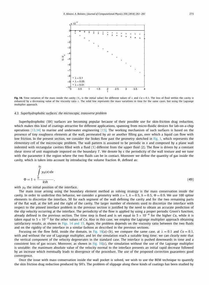
Fig. 14. Time variation of the mass inside the cavity (Vo is the initial value) for different values of λ and Ca = 0.1. The loss of fluid within the cavity is enhanced by a decreasing value of the viscosity ratio λ. The solid line represents the mass variations in time for the same cases, but using the Lagrange multiplier approach.

4.3. Superhydrophobic surfaces: the microscopic, transverse problem

Superhydrophobic (SH) surfaces are becoming popular because of their possible use for skin-friction drag reduction, which makes this kind of coatings attractive for different applications, spanning from micro-fluidic devices for lab-on-a-chip operations [13,14] to marine and underwater engineering [15]. The working mechanism of such surfaces is based on the presence of tiny roughness elements at the wall, permeated by air or another filling gas, over which a liquid can flow with low friction. In the present section, we consider the Stokes flow past the geometry sketched in Fig. 1, which represents the elementary cell of the microscopic problem. The wall pattern is assumed to be periodic in x and composed by a plane wall indented with rectangular cavities filled with a fluid (1) different from the upper fluid (2). The flow is driven by a constant shear stress of unit magnitude imposed on the boundary T . We denote by s the periodicity of the wall texture and we tune with the parameter k the region where the two fluids can be in contact. Moreover we define the quantity of gas inside the cavity, which is taken into account by introducing the volume fraction , defined as:

= 1 +

ks∫0

y0(x)dx

ksh, (49)

with y0 the initial position of the interface.The main issue arising using the boundary element method as solving strategy is the mass conservation inside the

cavity. In order to underline this behavior, we consider a geometry with s = 1, k = 0.5, h = 0.5, = 0.9. We use 100 spline elements to discretize the interface, 50 for each segment of the wall defining the cavity and for the two remaining parts of the flat wall, at the left and the right of the cavity. The larger number of elements used to discretize the interface with respect to the pinned interface problem in the previous section is justified by the need to obtain an accurate prediction of the slip velocity occurring at the interface. The periodicity of the flow is applied by using a proper periodic Green’s function, already defined in the previous section. The time step is fixed and is set equal to 5 × 10−4 for the higher Ca, while it is taken equal to 5 × 10−3 for the other values of Ca. Also in this case, we employ the Lagrange multiplier approach obtaining satisfactory results, as shown in Figs. 14 and 15. Again, the problem depends on the viscosity ratio between the two fluids and on the rigidity of the interface in a similar fashion as described in the previous sections.

Focusing on the flow field, inside the domain, in Fig. 16(a)–(b), we compare the same case, at λ = 0.1 and Ca = 0.1, with and without the use of Lagrange multiplier, and let the simulation reach a suitable long time; we can clearly note that the vertical component of the velocity degenerates in the standard case. The interface is pushed downwards in time and a consistent loss of gas occurs. Moreover, as shown in Fig. 16(c), the simulation without the use of the Lagrange multiplier is unstable: the maximum absolute value of the velocity normal to the interface presents an initial rapid decrease followed by an increase which eventually leads to divergence of the procedure. The use of the proposed correction guarantees good convergence.

Once the issue with mass conservation inside the wall pocket is solved, we wish to use the BEM technique to quantify the skin friction drag reduction produced by SH’s. The problem of slippage along these kinds of coatings has been studied by

274 E. Alinovi, A. Bottaro / Journal of Computational Physics 356 (2018) 261–281

Fig. 15. Time variation of the mass inside the cavity for different values of Ca and λ = 0.01. The loss of fluid within the cavity is enhanced by a decreasing value of the capillary number Ca. The solid line represents the mass variations in time for the same cases, but using the Lagrange multiplier approach.

Fig. 16. Vertical velocity field generated in the domain at t = 10. a) Standard implementation; b) Lagrange multiplier approach; c) history of the maximum absolute value of the velocity normal to the interface for the standard implementation (dashed line) and the Lagrange multiplier approach (solid line). (For interpretation of the references to color in this figure, the reader is referred to the web version of this article.)

E. Alinovi, A. Bottaro / Journal of Computational Physics 356 (2018) 261–281 275

Fig. 17. Comparison in transverse protrusion heights between the analytical model by Davis & Lauga [19] and the present numerical simulations. The solid lines correspond to the analytical model by Davis & Lauga for k = 0.3 (lower line), k = 0.5 (intermediate line), k = 0.7 (upper line). Symbols are the simulations, for the same values of k, with λ = 0.018 (�), λ = 0.05 (�), λ = 0.1 (◦). (a) Ca = 1; (b) Ca = 0.1.

different authors since the seminal work by Philip [16], who analyzed the flow along a flat wall patterned with alternating regions of no-slip and no-shear. What is known from analytical considerations [17,18], is that the velocity far from the rough walls, or with superhydrophobic patterned protrusions reads

u(y) = y + b (50)

where b is a constant known as transverse protrusion height or transverse slip length and represents the virtual distance below (or above) the x-axis where the u velocity component would extrapolate to zero. In the literature, there are several extensions of the work by Philip. In particular, Davis & Lauga [19] have proposed an analytical model for the slip length b in the presence of a curved meniscus, over which a perfect slip boundary condition is applied. In our numerical simulations, we maintain the same set-up shown in Fig. 1 and we calculate the slip length when varying the viscosity ratio, the capillary number, the length of the cavity k, and the volume ratio . According to our definition, > 0 means that the meniscus is protruding outside the cavity.

In Fig. 17 we propose a comparison between the analytical model and our numerical simulations. The agreement is good, especially for the values of k = 0.3 and k = 0.5, but this is not surprising, since the analytical model is valid in the dilute limit, i.e. for small values of k. If one compares the value of the slip length with k = 0.7 and flat interface ( = 1), the model

by Davis and Lauga yields b

s= 0.0963, while both Philip’s and our calculations give

b

s= 0.126. Increasing the viscosity ratio

λ has the effect of decreasing the slip length, since for small λ the approximation of perfect slip along the interface is better. The present simulations also confirm the existence of a critical value of for which the slip length becomes negative. This condition, already pointed out in refs. [20,21], occurs when the interface has an excessive protrusion outside of the cavity. The largest value of the protrusion height is found, almost independently of Ca and λ, when is close to 1.05, i.e. when the interface is very mildly protruding out of the cavity, and this is possibly the most promising condition in terms of the skin friction drag reduction. The definite answer can however come only from the resolution of the companion problem for the longitudinal protrusion height since, as shown by Luchini et al. [18], shear stress reduction at the wall depends to first order on the difference between longitudinal and transverse protrusion heights.

The interface deforms under the action of the shear flow as shown in Fig. 18, but for a sufficiently low capillary number it presents a very small deviation from the steady shape position that it would have in the absence of forcing flow. In particular, for < 1, the interface is quasi-parabolic, well approximated by equation (39), and for > 1 it assumes a position close to a circular arch, whose equation is reported in [19]. The flow field generated inside the domain are reported in Fig. 19 for both larger and smaller than one.

276 E. Alinovi, A. Bottaro / Journal of Computational Physics 356 (2018) 261–281

Fig. 18. Shape of the interface for Ca = 1 (left) and Ca = 0.1 (right) and λ = 0.1. The values of are 0.85, 0.90, 0.95, 1.10, 1.15, 1.25 and the flow is from left to right.

Fig. 19. Iso-contours of the streamwise and wall normal velocity for λ = 0.1 and Ca = 1. The value of the volume ratio is = 0.85 (a)–(b) and = 1.15(c)–(d). (For interpretation of the references to color in this figure, the reader is referred to the web version of this article.)

5. Conclusions

A novel method to enforce mass conservation in multiphase Stokes flows problems using the boundary element method has been presented. We have underlined how a viscosity ratio λ < 1 and the presence of a large interfacial tension cause issues in mass conservation, offering clear examples. The method proposed is based on an easy-to-implement modification of the linear system obtained by the discretization of the governing boundary integral equation, which consists in adding one constraint equations for the interfacial velocity for each interface inside the domain of interest, by the use of Lagrange multipliers. The technique is very effective in limiting the mass leakage/creation for all the benchmark problems considered. In comparison with the deflation method, introduced by Pozrikidis [6], it achieves a better convergence, reducing the maxi-mum absolute velocity normal to the interface by several orders of magnitude and ensuring mass conservation even in cases where the double-layer deflation approach fails. We have used our boundary element code to solve the problem of slippage over superhydrophobic surfaces, taking into account the effect of viscosity ratio and capillary number while computing the

E. Alinovi, A. Bottaro / Journal of Computational Physics 356 (2018) 261–281 277

Fig. 20. Sketch of two adjacent elements approximated by cubic splines. The • represent the collocations points defined at the end of each element.

deformation of the interface. The results are in good agreement with the theoretical predictions by Davis & Lauga [19] and confirm the presence of a maximum value of the slip length for a slightly protruding bubble.

Acknowledgements

This activity has started thanks to a gratefully acknowledged Fincantieri Innovation Challenge grant, monitored by Cetena S.p.A. The authors thank Giacomo Gallino for interesting discussions.

Appendix A. Numerical details on the boundary element method

In section 3 we have briefly described the numerical method employed in this paper, giving an extended explanation only of its major features. In this appendix, we will describe more extensively some numerical details. In particular, we consider the computation of the single-layer and the double-layer integral operators, which are the entries of the matrices S∗∗ and D∗∗ in equation (17).

The starting point is to define the shape of the boundary element, which, in our case, is a spline connecting two collo-cation points, as shown in Fig. 20. We define a curvilinear abscissa, s, over the element Ek and we recast the operators (2)and (3) as

F S L Pj (x0, u; Ek) =

s2∫s1

f ki [x(s)]G i j[x(s), x0]hk

s(s)ds (51)

F DL Pj (x0, u; Ek) =

s2∫s1

uki [x(s)]T i jl[x(s), x0]nl[x(s)]hk

s (s)ds, (52)

where hks (s) is the metric associated with the element:

hs(s) =[(

dx

ds

)2

+(

dy

ds

)2] 1

2

. (53)

We apply another coordinate transformation which maps an element from the global coordinate system based on the curvilinear abscissa to a local coordinate system such that the kth element’s boundary points are mapped onto the interval [−1, 1]. This mapping will result useful for the numerical quadrature of boundary integrals and can be simply carried out using the following relation:

s(ζ ) = (s1 + s2)

2+ (s2 − s1)

2ζ = sm + sdζ, (54)

from which we can easily define the associated metric hζ = sd . Introducing this new parametrization into the integrals (51)and (52) we obtain:

F S L Pj (x0, f ; Ek) = hk

ζ

1∫−1

f ki (x(s(ζ )))G i j(x(s(ζ )), x0)h

ks dζ, (55)

F DL Pj (x0, u; Ek) = hk

ζ

1∫−1

uki (x(s(ζ )))T i jk(x(s), x0)nk(x(s(ζ )))hk

sdζ. (56)

Until now, no assumption has been made on the interpolation method of the boundary quantities over the element. We use a piecewise linear variation, which is a good compromise between accuracy and programming difficulty; thus, let us consider an element parametrized using the local coordinate ζ , as show in Fig. 21, and require that:

u(ζ ) = ψ1(ζ )u1 + ψ2(ζ )u2, (57)

f (ζ ) = ψ1(ζ ) f 1 + ψ2(ζ ) f 2, (58)

278 E. Alinovi, A. Bottaro / Journal of Computational Physics 356 (2018) 261–281

Fig. 21. Schematic view of an element parametrized using local coordinates ζ : the red cross marks the position of the collocation points, while the black dot marks the starting and ending points of the element. (For interpretation of the references to color in this figure legend, the reader is referred to the web version of this article.)

Fig. 22. Sketch of two boundary patches, with several collocation point defined over them.

where ψ1 = l2 − ζ

Land ψ2 = l1 + ζ

Lare shape functions. Introducing relations (57) and (58) into the expression of the

single- and double-layer integrals, we can recast (55) and (56) as:

F S L Pj (x0, f ; Ek) = f k

i A1i j + f k+1

i A2i j, (59)

F DL Pj (x0, u; Ek) = uk

i B1i j + uk+1

i B2i j, (60)

where Anij and Bn

ij are know tensors of the form:

Anij = hk

ζ

1∫−1

ψn(ζ )G i j(ζ )hs(ζ )dζ, (61)

Bnij = hk

ζ

1∫−1

ψn(ζ )T i jl(ζ )nl(ζ )hs(ζ )dζ. (62)

The integrals (61) and (62) can be computed numerically by using the Gauss–Legendre quadrature rule, if the integrand is non-singular. The singular integral case is more tricky and special techniques must be employed, as extensively illustrated in the following section. We consider now two adjacent elements sharing the kth collocation point, as shown in Fig. 20, and we write down the following quantities

S Llk = A2

i j|k−1k + A1

i j|kk, (63)

D Llk = B2

i j|k−1k + B1

i j|kk, (64)

where in the notation |∗∗ the superscript stands for the element over which the integral is being evaluated, while the subscript represents the collocation point considered.

As an example, referring to Fig. 22, we consider the assembling of the influence matrix D P1 P2 relative to the double-layer potential operator for two arbitrary patches, called P1 and P2, with N P1 and N P2 collocation points, respectively.

The discretized double-layer operator D P1 P2 reads

D P1 P2 =

⎡⎢⎢⎢⎢⎢⎣

D L11 D L2

1 . . . D LN P21

D L12 D L2

2 . . . D LN P22

......

......

D L1N P1

D L2N P1

. . . D LN P2N P1

⎤⎥⎥⎥⎥⎥⎦ ; (65)

here D Llk stands for the quantities (64) calculated at the kth point belonging to P2 considering the lth collocation point

belonging to P1. Particular attention should be paid when a collocation point is not shared by two adjacent segments. In this case D Ll turns out to be

k

E. Alinovi, A. Bottaro / Journal of Computational Physics 356 (2018) 261–281 279

D Llk = B1

i j|kk, (66)

if the collocation point is located on the left of the element, while

D Llk = B2

i j|kk, (67)

if the collocation point is located on the right of the element. The assembling methodology is the same for other cases, with no difference in the procedure if we consider the single-layer potential.

Non-singular integrals

The integrals (61)–(62) are the building blocks for the numerical solution of the boundary integral equations. Let us recall the periodic velocity Green’s function and its associated stress tensor in order to highlight the problems that may arise in their numerical evaluation.

Starting from G i j :

A(x) = 1

2log{2[cosh(ω y) − cos(ωx)]}, (68)

G11 = −A(x) − y∂ A(x)

∂ y+ 1, (69)

G12 = y∂ A(x)

∂ x, (70)

G22 = A(x) + y∂ A(x)

∂ x, (71)

where x = x − x0 and ω = 2πL , with L the period of the flow. The components of the stress tensor T i jk are:

T111 = −4∂ A(x)

∂ x− 2 y

∂2 A(x)

∂ x∂ y, T112 = −2

∂ A(x)

∂ y− 2 y

∂2 A(x)

∂ y∂ y, (72)

T212 = 2 y∂2 A(x)

∂ x∂ y, T222 = −2

∂ A(x)

∂ y+ 2 y

∂2 A(x)

∂ y∂ y. (73)

If the point x0 does not lay over the same element for which we are performing the integration, integrals (61) and (62) are not singular and can be approximated using the Gauss–Legendre formula, using Nq quadrature points, as:

hkζ

1∫−1

ψn(ζ )G i j(ζ )hs(ζ )dζ = hkζ

Nq∑q=1

ψn(ζq)G i j(ζq)hs(ζq)wq, (74)

hkζ

1∫−1

ψn(ζ )G i j(ζ )hs(ζ )dζ = hkζ

Nq∑q=1

ψn(ζq)T i jl(ζq)nl(ζ )hs(ζq), (75)

where ζq is the position of the qth quadrature point along the interval [−1, 1] and wq is the associated weight.

Singular integrals

In the case of two-dimensional flows, as considered here, since the integrand of the double-layer potential exhibits a discontinuity across the collocation point x0 special accommodations are not necessary. In contrast, the single-layer potential exhibits a logarithmic singularity for the diagonal component of G . The basic idea to solve this problem is to subtract off the singularity. Thus, turning attention only to the term which contains the logarithm we add and subtract hsψ(s) log(r), r =|x − x0|, to the integrand in (51), obtaining:

− 1

2

s2∫s1

hs(s)ψn(s) log{2[cosh(ωx2) − cos(ωx1)]}ds =

− 1

2

[ s2∫s1

hs(s)ψn(s) log

{2

r[cosh(ωx2) − cos(ωx1)]

}+ hsψn(s) log(r)ds

]. (76)

280 E. Alinovi, A. Bottaro / Journal of Computational Physics 356 (2018) 261–281

The first term of the integrand is non-singular and can be accurately computed by Gauss–Legendre quadrature, but the second term involving log(r) is still singular and further manipulations are necessary. Calling s0 the curvilinear abscissa of the singular point, we add and subtract hs(s)ψn(s)log(|s − s0|) and recast the integral as:

s2∫s1

hsψn(s) log(r)ds =s2∫

s1

hs(s)ψn(s) log

(r

|s − s0|)

ds +s2∫

s1

hsψn(s)log(|s − s0|)ds. (77)

Again, the first term in the integrand is non-singular, but we must proceed to de-singularize the second term:

s2∫s1

hs(s)ψn(s)log(|s − s0|)ds =s2∫

s1

[hsψn(s) − hs(s0)ψn(s0)

]log(|s − s0|)ds +

s2∫s1

hs(s0)ψn(s0) log(|s − s0|)ds. (78)

Finally we can conclude the de-singularization noting that hs(s0)ψn(s0) is constant thus:

s2∫s1

hs(s0)ψn(s0) log(|s − s0|)ds = hs(s0)ψn(s0)[|s2 − s0|

(log(|s2 − s0|) − 1

) + |s1 − s0|(

log(|s1 − s0|) − 1)]

. (79)

Summing up, we can compute numerically the singular integral on the left-hand-side of (76) as:

− 1

2

s2∫s1

hs(s)ψn(s) log{2[cosh(ωx2) − cos(ωx1)]}ds =

−Nq∑

q=1

hζ wq

2

[hs(ζq)ψn(ζq) log

{2

r[cosh(ωx2(ζq)) − cos(ωx1(ζq))]

}+

hs(ζq)ψn(ζq) log

(r

|s(ζq) − s0|)

+ [hs(ζq)ψn(ζq) − hs(s0)ψn(s0)

]log(|s(ζq) − s0|)

]−

hs(s0)ψn(s0)

2

(|s2 − s0|

(log(|s2 − s0|) − 1

) + |s1 − s0|(

log(|s1 − s0|) − 1))

.

References

[1] M. Kennedy, C. Pozrikidis, R. Skalak, Motion and deformation of liquid drops, and the rheology of dilute emulsions in simple shear flow, Comput. Fluids 23 (2) (1994) 251–278, https://doi.org/10.1016/0045-7930(94)90040-X.

[2] M. Loewenberg, E. Hinch, Numerical simulation of a concentrated emulsion in shear flow, J. Fluid Mech. 321 (1996) 395–419, https://doi.org/10.1017/S002211209600777X.

[3] I.B. Bazhlekov, P.D. Anderson, H.E. Meijer, Nonsingular boundary integral method for deformable drops in viscous flows, Phys. Fluids 16 (4) (2004) 1064–1081, https://doi.org/10.1063/1.1648639.

[4] M. Nemer, X. Chen, D. Papadopoulos, J. Bławzdziewicz, M. Loewenberg, Hindered and enhanced coalescence of drops in Stokes flows, Phys. Rev. Lett. 92 (11) (2004) 114501, https://doi.org/10.1103/PhysRevLett.92.114501.

[5] M. Nagel, F. Gallaire, Boundary elements method for microfluidic two-phase flows in shallow channels, Comput. Fluids 107 (2015) 272–284, https://doi.org/10.1016/j.compfluid.2014.10.016.

[6] C. Pozrikidis, Expansion of a compressible gas bubble in Stokes flow, J. Fluid Mech. 442 (2001) 171–189, https://doi.org/10.1017/S0022112001004992.[7] C. Pozrikidis, Boundary Integral and Singularity Methods for Linearized Viscous Flow, Cambridge University Press, 1992.[8] C. Pozrikidis, A Practical Guide to Boundary Element Methods with the Software Library BEMLIB, CRC Press, 2002.[9] J. Tanzosh, M. Manga, H. Stone, Boundary integral methods for viscous free-boundary problems: deformation of single and multiple fluid-fluid inter-

faces, in: C.A. Brebbia, M.S. Ingber (Eds.), Boundary Element Technology VII, Springer, 1992, pp. 19–39.[10] C. Pozrikidis, BEMLIB, http://dehesa.freeshell.org/BEMLIB/.[11] OpenFOAM, The open source CFD toolbox, User Guide, http://www.openfoam.org, 2015.[12] C.W. Hirt, B.D. Nichols, Volume of fluid (VoF) method for the dynamics of free boundaries, J. Comput. Phys. 39 (1) (1981) 201–225, https://doi.org/

10.1016/0021-9991(81)90145-5.[13] H.A. Stone, A.D. Stroock, A. Ajdari, Engineering flows in small devices: microfluidics toward a lab-on-a-chip, Annu. Rev. Fluid Mech. 36 (2004) 381–411,

https://doi.org/10.1146/annurev.fluid.36.050802.122124.[14] T.M. Squires, S.R. Quake, Microfluidics: fluid physics at the nanoliter scale, Rev. Mod. Phys. 77 (3) (2005) 977, https://doi.org/10.1103/RevModPhys.

77.977.[15] H. Dong, M. Cheng, Y. Zhang, H. Wei, F. Shi, Extraordinary drag-reducing effect of a superhydrophobic coating on a macroscopic model ship at high

speed, J. Mater. Chem. A 1 (19) (2013) 5886–5891, https://doi.org/10.1039/C3TA10225D.[16] J.R. Philip, Flows satisfying mixed no-slip and no-shear conditions, Z. Angew. Math. Phys. ZAMP 23 (3) (1972) 353–372, https://doi.org/10.1007/

BF01595477.[17] D. Bechert, M. Bartenwerfer, The viscous flow on surfaces with longitudinal ribs, J. Fluid Mech. 206 (1989) 105–129, https://doi.org/10.1017/

S0022112089002247.[18] P. Luchini, F. Manzo, A. Pozzi, Resistance of a grooved surface to parallel flow and cross-flow, J. Fluid Mech. 228 (1991) 87–109, https://doi.org/10.

1017/S0022112091002641.

E. Alinovi, A. Bottaro / Journal of Computational Physics 356 (2018) 261–281 281

[19] A.M. Davis, E. Lauga, Geometric transition in friction for flow over a bubble mattress, Phys. Fluids 21 (1) (2009) 011701, https://doi.org/10.1063/1.3067833.

[20] A. Steinberger, C. Cottin-Bizonne, P. Kleimann, E. Charlaix, High friction on a bubble mattress, Nat. Mater. 6 (9) (2007) 665–668, https://doi.org/10.1038/nmat1962M3.

[21] M. Sbragaglia, A. Prosperetti, Effective velocity boundary condition at a mixed slip surface, J. Fluid Mech. 578 (2007) 435–451, https://doi.org/10.1017/S0022112007005149.