Journal of Computational Physics 405 (2020) 109096

Contents lists available at ScienceDirect

Journal of Computational Physics

www.elsevier.com/locate/jcp

A two-way coupled Euler-Lagrange method for simulating

multiphase flows with discontinuous Galerkin schemes on

arbitrary curved elements

Eric J. Ching a,∗, Steven R. Brill b, Michael Barnhardt c, Matthias Ihme a

a Department of Mechanical Engineering, Stanford University, Stanford, CA 94305, USAb Institute for Computational and Mathematical Engineering, Stanford University, Stanford, CA 94305, USAc NASA Ames Research Center, Mountain View, CA 94035, USA

a r t i c l e i n f o a b s t r a c t

Article history:Received 1 February 2019Received in revised form 16 October 2019Accepted 3 November 2019Available online 11 November 2019

Keywords:Discontinuous Galerkin methodLagrangian particle trackingParticle-laden flowHypersonic flowCurved elementsDusty flow

In this work, we develop a Lagrangian point-particle method to support high-speed dusty flow simulations with discontinuous Galerkin schemes. The carrier fluid is treated in an Eulerian frame through the solution of the compressible Navier-Stokes equations. Particle search and localization is based on the geometric mapping of mesh elements to a reference element and is applicable to arbitrary unstructured, curved, multidimensional grids. High-order interpolation is used to calculate the gas state at a given particle position, and the back-coupling of particles to the carrier fluid is carried out via a simple, effective procedure. Furthermore, we discuss difficulties associated with accounting for particle-wall collisions on curved, high-aspect-ratio elements. We develop a methodology that appropriately handles such collisions and accurately computes post-collision particle trajectories. We first apply the Euler-Lagrange method to one-way coupled tests and show the benefit of using curved instead of straight-sided elements for dealing with particle-wall collisions. We proceed by considering more complex multiphase test cases with two-way coupling, namely dusty flows over a flat plate and through a converging-diverging nozzle. Our final test case consists of hypersonic dusty flow over a sphere in which the target quantity is dust-induced surface heating augmentation at the stagnation point. Quantitative comparisons with experiments are provided.

© 2019 Elsevier Inc. All rights reserved.

1. Introduction

Compressible particle-laden flows can be observed in a wide range of applications, such as spray coating [1], dust-induced boundary layer transition in atmospheric flight [2], dust detonations [3], and interactions between solid particulates and vehicle exhaust plumes [4,5]. Another prominent example is the enhancement of erosion, augmentation of surface heat fluxes, and other detrimental phenomena caused by solid particles in high-speed flows over blunt bodies. This is particularly relevant to Mars entry missions, given the high levels of dust particles suspended in the Martian atmosphere [6].

Different approaches for simulating multiphase flows have been developed, which can typically be classified as either Euler-Euler (EE) or Euler-Lagrange (EL) [7]. In EE schemes, such as the popular two-fluid model, both the particles and the

* Corresponding author.E-mail address: eching@stanford.edu (E.J. Ching).

https://doi.org/10.1016/j.jcp.2019.1090960021-9991/© 2019 Elsevier Inc. All rights reserved.

2 E.J. Ching et al. / Journal of Computational Physics 405 (2020) 109096

carrier fluid are described in an Eulerian frame as continuous phases. Despite the comparably low computational cost, EE schemes may often suffer from inadequate descriptions of very dilute flows [8], polydisperse flows [9–11], and particles with large Stokes numbers [12]. Nevertheless, recent studies have focused on overcoming some of the difficulties associated with EE schemes [8,13,14]. In contrast, EL strategies encompass a wide range of approaches in which the disperse phase is tracked in a Lagrangian manner. In fully resolved EL simulations, the flow field around each particle is accurately computed [15]; however, the grid resolution required to capture the smallest scales near particle surfaces limits these simulations to low number densities and simple configurations. Alternatively, point-particle approaches, such as the particle-source-in-cell (PSIC) method [7], are commonly employed. These methods typically rely on the assumption that particle sizes are small compared to the characteristic length scale of the carrier fluid. Particles acts as point sources in the Eulerian solver, and momentum and thermal exchange is based on the immediate carrier fluid state. This enables the simulation of a very large number of particles while maintaining a satisfactory degree of accuracy. Akiki et al. [16] recently developed the pairwise interaction extended point-particle (PIEP) model, which computes the force and torque on a given particle taking into account the arrangement of nearby particles. In this paper, we focus on Lagrangian point-particle tracking.

Multiphase flow simulations can be further characterized by the level of interphase and intraphase coupling, as discussed in Ref. [7]. In one-way coupled simulations, particles are influenced by the carrier fluid, but not vice-versa. This is appro-priate for low mass and volume loadings. Although these simulations in general are not especially challenging, accurate interpolation of the carrier fluid and reliable time stepping strategies are needed to obtain good results [17,18]. Two-way coupling signifies the interaction between both the disperse phase and the carrier phase, typically employed in moderately dilute flows with high mass concentrations. The particle-to-fluid coupling can pose difficulties; for instance, the influence of particles must be appropriately translated to the carrier phase to maintain accuracy and prevent numerical instabilities [19–21]. Finally, in the four-way coupling regime, where flows are dense, particles interact with each other via collisional, cohesive, van der Waals, lubrication, electrostatic, and other forces [22]. These simulations usually employ a collision detec-tion algorithm [21,23] in which each particle is aware of nearby particles, resulting in higher computational costs.

The majority of particle-laden CFD simulations have been performed using low-order finite-volume (FV) or finite-difference (FD) schemes due to their simplicity. However, the complex physics prevalent in these applications (even in the absence of particles) provides an opportunity for high-order numerical methods to excel. A number of high-order FD [20] and spectral-based [24,16] simulations of particle-laden flows can be found in the literature. However, these numer-ical schemes can be difficult to apply to high-aspect-ratio elements on unstructured meshes. Discontinuous Galerkin (DG) schemes constitute an increasingly popular family of numerical methods that combines elements of classical finite element (FE) and FV techniques. DG schemes exhibit many favorable properties, including high-order accuracy, low dissipation and dispersion errors [25,26], compatibility with unstructured grids and complex geometries, hp-adaptation capabilities, and straightforward parallelization. Specifically in the context of particle tracking, curved meshes, which are frequently em-ployed in high-order solution discretizations, can potentially improve the prediction of particle trajectories in cases where particle-wall collisions are important.

In recent years, progress has been made in applying DG schemes to particle-laden flow problems. Sabat et al. [27] applied a DG discretization to an Eulerian formulation of the disperse phase. They applied their model in a one-way coupled fashion to a frozen velocity field in homogeneous isotropic turbulence computed with an FD solver. Ejtehadi et al. [9] discretized the two-fluid model equations in a DG framework and analyzed wave patterns in multiphase explosion, double Mach reflec-tion, and underexpanded jet problems. With regard to EL methods, Banerjee et al. [28] have developed a one-way coupled Lagrangian particle solver in a DG formulation. In the field of plasma dynamics, Jacobs and Hesthaven [19,29] presented a particle-in-cell (PIC) algorithm coupled with a DG solver for Maxwell’s equations. The PIC scheme uses high-order interpo-lation of the electromagnetic field, smooth shape functions for weighing particles to the Eulerian mesh, and techniques to enforce charge conservation. They applied the formulation to 2D straight-sided meshes, exploiting the analytical inverse of the geometric mapping for particle localization and relying on a level-set distance function to handle particle-wall collisions. The PIC method has been extended and applied to several plasma problems [30–32]. On the whole, however, there has not been substantial development of EL strategies for computing particle-laden fluid flows on arbitrary curved meshes.

As such, the objective of this work is to develop a two-way coupled Lagrangian point-particle solver for DG schemes. We concentrate on dilute gas-solid compressible flows with large numbers of small particles. A major focus of our method is the ability to handle particle-wall collisions (based on the hard-sphere model [7]) on arbitrary curved, high-aspect-ratio elements. This is significantly more challenging than on straight-sided meshes since the intersection between a given par-ticle trajectory and the wall cannot be calculated analytically. Furthermore, a number of pathological situations can occur that require adequate treatment to ensure physical consistency. Particle search and localization is based on the geometric mapping from physical elements to a reference element, coupled with efficient search strategies [33]. High-order polynomi-als are used to interpolate the carrier phase state to the particles. To translate the effect of particles on the Eulerian carrier fluid solver, we employ Dirac delta functions. This results in a simple two-way coupling procedure that, in addition to being sufficiently effective for our targeted flow configurations, circumvents additional challenges associated with curved, high-aspect-ratio elements. We have implemented the resulting Lagrangian particle method in a high-order parallel DG solver capable of simulating viscous high-speed flows [34].

The remainder of the paper is organized as follows: Section 2 outlines the governing equations and DG discretization, followed by a description of the particle solver in Section 3. The subsequent section focuses on results for a variety of test cases. We begin with one-way coupled simulations to verify the tracking algorithms and demonstrate the benefits of

E.J. Ching et al. / Journal of Computational Physics 405 (2020) 109096 3

utilizing curved (instead of linear) meshes. We continue by focusing on a series of more complex two-way coupled tests, culminating in application to hypersonic dusty flow over a blunt body. In this problem, we are interested in dust-induced heat flux augmentation and compare our DG results to experimental data. The paper concludes with a summary of the main contributions and a discussion of potential future improvements.

2. Mathematical formulation of carrier fluid

2.1. Governing equations of the carrier phase

The behavior of the carrier phase is described by the governing equations for conservation of mass, momentum, and total energy as

∂tU + ∇ · Fs = ∇ · Fv + S, (1)

where U(x, t) : RND × R → RNU is the conservative state vector, Fs(U) : RNU → RNU ×ND is the inviscid flux vector, Fv(U, ∇U) : RNU × RNU ×ND → RNU ×ND is the viscous flux vector, and S(U, ∇U) : RNU × RNU ×ND → RNU is the source term vector. In addition, x ∈RND is the spatial coordinate vector, t is the time, NU is the number of state variables, and ND

is the number of spatial dimensions. The individual terms in Eq. (1) take the following form:

U =⎡⎣ ρ

ρuρE

⎤⎦ , Fs =⎡⎣ ρu

ρu ⊗ u + PI

u(ρE + P )

⎤⎦ , Fv =⎡⎣ 0

τu · τ − q

⎤⎦ , S =⎡⎣ Sρ

Sm

Se

⎤⎦ , (2)

where ρ is the density, u is the velocity vector, P is the thermodynamic pressure, E is the total energy per unit mass, and I is the identity matrix. Sρ , Sm , and Se are source terms representing the influence of particles on the carrier gas. The viscous stress tensor and heat flux are given as

τ = μ[∇u + (∇u)T ] − 2

3μ(∇ · u)I, (3a)

q = −κ∇T , (3b)

respectively. In Eq. (3a), μ is the dynamic viscosity, obtained using Sutherland’s law,

μ = μref

(T

Tref

)1.5 Tref + Ts

T + Ts, (4)

where μref is the viscosity at the reference temperature Tref and Ts is the Sutherland constant. In addition, κ = cpμ/Pris the thermal conductivity, with Pr being the Prandtl number and cp = Rγ /(γ − 1) the specific heat capacity at constant pressure. R is the specific gas constant and γ , the specific heat ratio, is set to a value of 1.4 in this study. Note that Eqs. (2)assume the volume fraction of the disperse phase to be small. By the ideal gas law, pressure is related to internal energy as

P = (γ − 1)(ρE − ρ

2|u|2

). (5)

2.2. Discontinuous Galerkin discretization

To develop a discontinuous Galerkin formulation, the problem is considered to be posed on the computational domain � with boundary ∂�. � is partitioned into Ne non-overlapping discrete elements such that � = ∪Ne

e=1�e . The boundary of element �e is denoted by ∂�e . The global space of test functions is defined as

V = ⊕Nee=1Ve, Ve = span {φm(�e)}Nb

m=1 , (6)

with φm the mth polynomial basis and Nb the number of basis functions. The global solution U is approximated by U , such that

U ≈ U = ⊕Nee=1U e. (7)

The local solution approximation U e ∈ Ve is given by

U e(t, x) =Nb∑

Uen(t)φn(x), (8)

n=1

4 E.J. Ching et al. / Journal of Computational Physics 405 (2020) 109096

and the basis coefficients Ue(t) ∈RNU ×Nb are obtained from the discretized solution of

Nb∑n=1

dt Uen(t)

∫�e

φmφnd�e +∫�e

φm∇ · F sd�e =∫�e

φm∇ · F vd�e +∫�e

φm Sd�e ∀ φm, (9)

where m = 1, ..., Nb . F s , F v , and S are the approximations to Fs , Fv , and S, respectively.To solve the variational formulation in Eq. (9), integration by parts is performed on the convective and viscous terms,

resulting in the emergence of surface integrals through which boundary and interface conditions are imposed. In this study, Roe’s approximate Riemann solver [35] and the BR2 scheme [36] are employed to define the convective flux and viscous flux contributions, respectively. We use Lagrange polynomials for the basis and test functions. To evaluate integrals, we use standard Gaussian quadrature with an order of accuracy no less than 2p + 1, where p is the order of the Lagrange interpolants. In addition, to capture shocks, intraelement pressure variations are used for shock detection while smooth artificial viscosity is used for stabilization, following the method developed in Ref. [34].

3. Particle solver

In this section, we describe the Lagrangian point-particle method for computing the behavior of the disperse phase in the flow field. We begin by outlining the main simplifying assumptions in our model. Individual particles are treated as smooth, solid, non-rotating, inert spheres with fixed diameters that exchange only momentum and energy with the carrier phase, i.e. Sρ = 0. We assume that particles do not interact with each other and that the temperature of a given particle is uniform over the entire particle. Furthermore, we assume that any turbulence generation due to the particles is negligible. The disperse phase is considered to be dilute.

The remainder of this section discusses the particle governing equations, high-order interpolation strategy, tracking algo-rithm, two-way coupling methodology, and treatment of particle-wall collisions.

3.1. Disperse phase governing equations

The state of a given particle is computed using the following set of ordinary differential equations [7]:

dxd

dt= ud, (10a)

mddud

dt= F , (10b)

mdcddTd

dt= Q , (10c)

where we introduce the subscripts “c” and “d” to represent the carrier and disperse phases, respectively. xd = [xd, yd, zd]T

is the particle position, ud = [ud, vd, wd]T is the particle velocity, md = πρd D3/6 is the particle mass (with ρd the particle density and D the particle diameter), cd is the specific heat of the particle, and Td is the particle temperature. F and Q are the overall force and convective heating rate on the particle, respectively. In this study, F = F qs + F thermo and Q = Q qs , where F qs is the quasi-steady drag, Q qs is the quasi-steady heating rate, and F thermo is the thermophoretic force. This force acts in the opposite direction of the temperature gradient and is induced by greater molecular velocities on the higher-temperature side than on the lower-temperature side of the particle [37]. As is typical in the modeling of gas flows with small solid particles [7,38], given the disparate densities of the two phases, we ignore additional contributions to F such as the stress-gradient, virtual mass, Basset history, Faxen, Saffman lift, buoyancy, and electrostatic forces [7,39]. Similarly, we ignore undisturbed-unsteady, diffusive-unsteady (history), radiation, and other contributions to Q [7,39]. The quasi-steady drag and heating rate are defined as

F qs = 1

8π D2ρc(uc − ud)|uc − ud|C D , (11a)

Q qs = π Dκc(Tc − Td)Nu, (11b)

respectively. In this work, we employ different correlations for the drag coefficient, C D , and the Nusselt number, Nu. These are dependent on the relative particle Reynolds number and the relative particle Mach number, defined as

Rep = ρc|uc − ud|Dμc

, (12a)

Map = |uc − ud|√γ RTc

. (12b)

The exact forms of C D and Nu will be further detailed in Section 4. Note that in all test cases except that described in Section 4.3, we set F thermo = 0.

E.J. Ching et al. / Journal of Computational Physics 405 (2020) 109096 5

3.2. Interpolation

To calculate F and Q in Eqs. (11) for a given particle, the carrier phase state must be evaluated at the particle position using an interpolation strategy. Various studies have demonstrated the importance of accurate interpolation in Lagrangian particle tracking [17,18]. It has further been found that in two-way coupled simulations, the order of the interpolation should match the formal order of accuracy of the spatial discretization [19,24]. As such, we exploit the subcell nature of the DG solution and compute the carrier phase state at the particle position xd with the same basis functions used to construct the local solution approximation. This results in a simple interpolation procedure that requires minimal implementation effort.

3.3. Two-way coupling methodology

The effect of the particles is translated to the flow field via the source term vector S = [0, Sm, Se]T on the RHS of Eq. (1), where

Sm = −N p∑i=1

F iχ(x − xd,i), (13a)

Se = −N p∑i=1

(Q i + ud,i · F i

)χ(x − xd,i). (13b)

These source terms represent the cumulative effect of the disperse phase on the fluid momentum and energy. The second term in Eq. (13b) is the work done by the overall particle drag and Np is the total number of particles. χ(x − xd,i) is a projection kernel that weighs the particle influence to the flow field and satisfies the property

∫�

χd� = 1. In this work, χ(x − xd,i) = δ(x − xd,i), the Dirac delta function. By using this choice of kernel, the source term in Eq. (9) can be evaluated in �e analytically as

∫�e

φm Sd�e =Ne

p∑i=1

φm(xd,i)[0, F i, Q i + ud,i · F i]T , (14)

where Nep is the number of particles located in element �e . This creates a straightforward two-way coupling methodology

with subcell-varying source-term contributions. In Refs. [19] and [20], smooth kernels, including Gaussian, polynomial, trun-cated cosine, and spline functions, were considered on the basis of reducing Gibbs-type instabilities. Since the present work largely focuses on the ability to handle particle-wall collisions on curved, high-aspect-ratio meshes, we favor the simplicity of the Dirac delta function, although extending smooth kernels to such mesh topologies will be the subject of future work. In our simulations, where we are interested in the overall effect of high concentrations of small particles, we find the Dirac delta function to perform sufficiently well and do not observe any associated instabilities.

3.4. Particle clouds

To reduce the computational cost, we represent a cloud of particles as a computational parcel [7]. When integrating Eq. (10) in time, we treat each particle cloud (parcel) as just an individual particle. However, particle mass concentrations, back-coupling of the disperse phase to the carrier phase, and energy transfer due to particle-wall collisions (discussed in Section 3.7) must be scaled accordingly. This increases the computational feasibility of simulating a considerable number of particles while maintaining acceptable modeling fidelity, assuming that each particle cloud does not represent an excessive number of physical particles. For clarity, we simply use “particles” to refer to particle clouds for the remainder of this paper.

3.5. Particle search-locate algorithm

As discussed previously, the state of the carrier phase must be interpolated at the particle position in solving Eqs. (10). This involves not only identifying the host element of each particle but also mapping the physical position of the particle, xd , to its reference position associated with the parent element, ξd . For DG schemes, in which unstructured grids with curved elements are used, this can present a major challenge. A variation of the algorithm presented by Allievi and Bermejo [33] is thus employed. This search and localization algorithm exploits the geometric mapping of elements already used in DG formulations. We summarize it here for q = 2 quadrilaterals in 2D, where q is the order of the geometry. The extension to 3D follows directly.

Let � denote the reference quadrilateral element such that

� ={[ξ,η]T | − 1 ≤ ξ,η ≤ 1

}. (15)

6 E.J. Ching et al. / Journal of Computational Physics 405 (2020) 109096

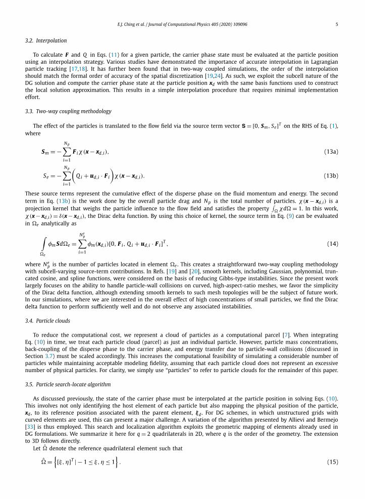
Fig. 1. Geometric mapping for q = 2 quadrilaterals.

Then, letting ξ = [ξ, η]T , the geometric mapping Le : � → �e is given as

Le(ξ) ≡[

xy

]=

Nn∑i=1

i(ξ)

[xe

iye

i

], (16)

where {[xei , y

ei ]T }Nn

i=1 denotes the physical coordinates of the Nn geometric nodes of �e and { i}Nni=1 are the basis functions

for the geometric interpolation. This is illustrated schematically in Fig. 1. With a standard Lagrange basis, the Nn = 9 basis functions for a q = 2 reference quadrilateral element are given by

1(ξ) = 14 ξη(1 − ξ)(1 − η),

3(ξ) = 14 ξη(1 + ξ)(1 + η),

5(ξ) = 12η(1 − ξ2)(η − 1),

7(ξ) = 12η(1 − ξ2)(η + 1),

9(ξ) = (1 − ξ2)(1 − η2),

2(ξ) = 14 ξη(1 + ξ)(η − 1),

4(ξ) = 14 ξη(ξ − 1)(1 + η),

6(ξ) = 12 ξ(1 + ξ)(1 − η2),

8(ξ) = 12 ξ(ξ − 1)(1 − η2).

(17)

If a point xd = [xd, yd]T ∈ � is in �e , then there exists ξd = [ξd, ηd]T ∈ � such that

G(ξd) ≡ xd − Le(ξd) = 0. (18)

Note that in general, solving Eq. (18) for ξd cannot be done analytically. As such, Newton’s method is employed in the following fashion: letting ξ0 ∈ � be an initial guess, for k = 0, . . . , Nk − 1, solve

ξk+1 = ξk − J −1e (ξk)G(ξk). (19)

Here, Nk is the number of Newton iterations until either convergence or another stopping criterion is reached, and J −1e (ξ)

is the inverse of the Jacobian matrix of the mapping Le , i.e. J e(ξ ) = ∂Le∂ξ . If convergence is attained and ξ Nk ∈ � according

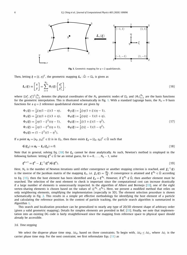
to Eq. (15), then the host element has been identified and ξd = ξ Nk . However, if ξ Nk /∈ �, then another element must be searched. The selection of the next element to check is important since the computational cost can increase drastically if a large number of elements is unnecessarily inspected. In the algorithm of Allievi and Bermejo [33], one of the eight vertex-sharing elements is chosen based on the values of (ξ Nk , ηNk ). Here, we present a modified method that relies on only neighboring elements, simplifying the implementation (especially in 3D). The element selection procedure is shown schematically in Fig. 2. This results in a simple yet effective methodology for identifying the host element of a particle and calculating the reference position. In the context of particle tracking, the particle search algorithm is summarized in Algorithm 1.

This search and localization procedure can be generalized to nearly any type of 2D/3D element shape of arbitrary order (given a valid geometric mapping). Details for simplex elements are provided in Ref. [33]. Finally, we note that implemen-tation into an existing DG code is fairly straightforward since the mapping from reference space to physical space should already be accessible.

3.6. Time stepping

We select the disperse phase time step, �td , based on three constraints. To begin with, �td ≤ �tc , where �tc is the carrier phase time step. For the next constraint, we first reformulate Eqs. (11) as

E.J. Ching et al. / Journal of Computational Physics 405 (2020) 109096 7

Fig. 2. Instructions for selecting next element to search based on values of the reference position ξ = (ξ,η).

Algorithm 1: Search-locate scheme for a given particle. �s denotes the element selected for inspection.Initialization: Set �s to be the host element of the particle from the previous time stepFound ← Falsewhile Found = False do

Perform Newton’s method on �s

if Newton’s method converges and ξ Nk ∈ � thenξd = ξ Nk

Found = Trueelse

Select new �s according to Fig. 2end

end

F qs = md

τm(uc − ud), (20a)

Q qs = mdcd

τe(Tc − Td), (20b)

where τm and τe are particle momentum and energy relaxation times, respectively. For stability, we limit �td such that �td < λτm and �td < λτe , where λ depends on the time stepping scheme. This is evaluated only for particles not already in equilibrium with the carrier fluid.

The last constraint is a CFL-like restriction, given as

�td ≤ h

max(1, p)

1

|ud| , (21)

where h is an element-based length scale and p is the polynomial order, which is incorporated to account for the subcell resolution of DG schemes. For cases in which the second and/or third constraints severely limit �td (for example, when deal-ing with particles with very small Stokes numbers), substepping can be employed, where multiple disperse-phase time steps are taken within one carrier-phase time step. For time stepping of the disperse phase, we typically use Adams-Bashforth (AB) time stepping due to the potential for high-order accuracy and low computational cost [18]. Runge-Kutta (RK) schemes can also be applied, but the interpolation, temporal integration, and search/localization steps must be performed at each stage, resulting in noticeably higher computational complexity.

3.7. Particle-wall collisions

We proceed by discussing the methodology for handling particle-wall interactions based on the hard-sphere model. Many existing schemes dealing with particle-wall collisions utilize a level set function corresponding to the signed distance from the wall [19,21]. However, this is not always appropriate for extremely high-aspect-ratio curved elements near the wall. Accordingly, just as for the particle search/localization scheme, we again rely directly on the geometric mapping from physical space to reference space, except we concentrate here on element faces. This is described below for q = 2 triangular and quadrilateral elements in 2D, where the faces consist of curves.

3.7.1. Newton searchLet � denote the reference line segment such that

� = {ζ | − 1 ≤ ζ ≤ 1} . (22)

8 E.J. Ching et al. / Journal of Computational Physics 405 (2020) 109096

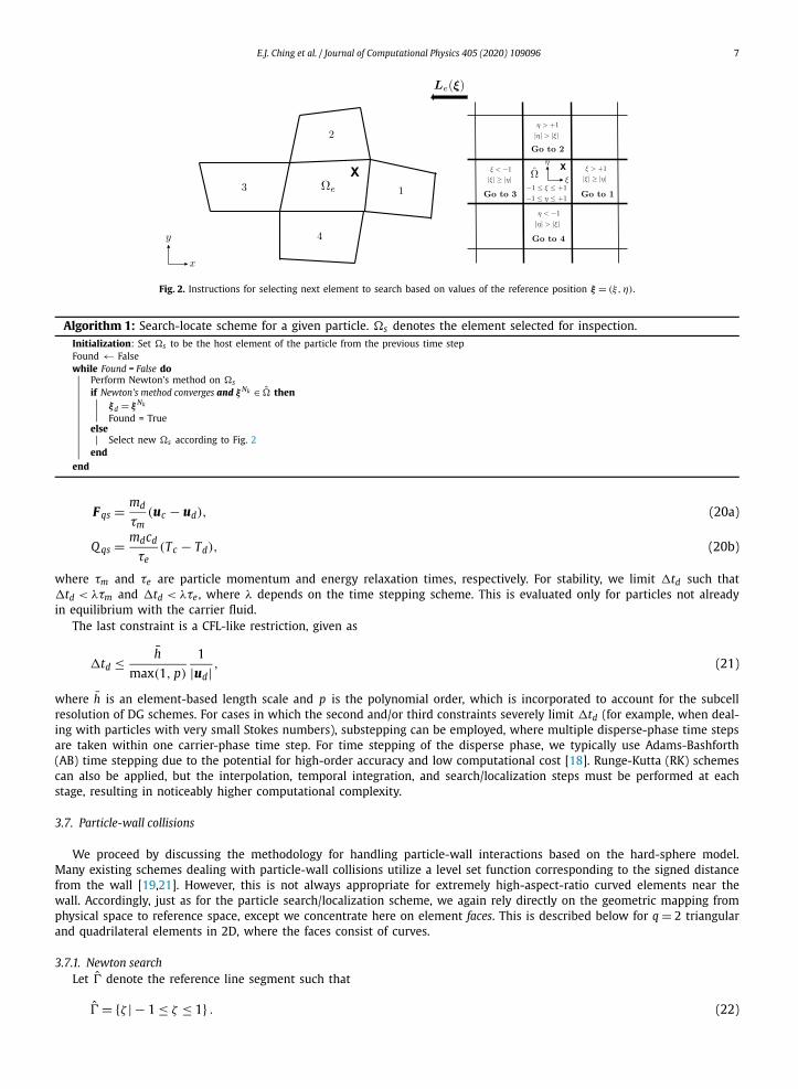
Fig. 3. Geometric mapping for q = 2 curves.

The geometric mapping H f : � → � f , where � f represents a given (curved) boundary face, takes the form

H f (ζ ) ≡[

xy

]=

Nm∑i=1

ψi(ζ )

[xe

iye

i

], (23)

where {[xei , y

ei ]T }Nm

i=1 are the physical coordinates of the Nm geometric nodes of � f and {ψi}Nmi=1 are the basis functions for

the geometry interpolation. Fig. 3 provides a schematic of this geometric mapping.The Nm = 3 standard Lagrange basis functions for q = 2 curves are defined as

ψ1(ζ ) = 1

2ζ(ζ − 1), (24a)

ψ2(ζ ) = 1

2ζ(ζ + 1), (24b)

ψ3(ζ ) = 1 − ζ 2. (24c)

Next, we approximate the particle trajectory, r, in a given time step as a line segment, which is valid given the small size of particles relative to characteristic element length scales. This trajectory can be parametrized as

rn(s) = xn−1d + ans, (25)

where an = xnd − xn−1

d is the particle displacement in the time step �t = tn − tn−1 (with n being the time index) and s ∈ [0, 1]. s = 0 and s = 1 correspond to tn−1 and tn , respectively. If the particle trajectory intersects � f , then there exist ζd ∈ � and sd ∈ (0, 1] such that

I ≡ H f (ζd) − r(sd) = 0, (26)

where we have dropped the superscript “n” for brevity. We use Newton’s method to solve Eq. (26). To this end, we linearize Eq. (26) and obtain the following recursion equation:

[ζ

s

]k+1

=[ζ

s

]k

−

⎡⎢⎢⎣∂ I1

∂ζ

∂ I1

∂s∂ I2

∂ζ

∂ I2

∂s

⎤⎥⎥⎦−1

∣∣∣∣∣∣∣∣∣(ζ,s)k

[I1I2

]k

, (27)

where k = 0, . . . , Nk −1. Nk is the total number of iterations, and ζ 0 and s0 are initial guesses. The inverse of the Jacobian in Eq. (27) can be calculated analytically. If Newton’s method converges, ζ Nk ∈ �, and sNk ∈ (0, 1], then the particle trajectory crosses the boundary face at ζw = ζ Nk (or equivalently, sw = sNk ). H f (ζw) = r(sw) gives the intersection point in physical space at which the particle collides with the wall.

Note that for straight-sided elements, the above Newton search procedure can still be applied, requiring fewer iterations to determine the intersection point than for curved elements. Alternatively, analytical formulas for calculating the intersec-tion between two lines (in 2D) or between a line and a plane (in 3D) can be used. The resulting intersection point, if it exists, must be inspected for whether it is inside or outside the linear/planar boundary face.

Since there is no need for an iterative procedure when using straight-sided elements, it may be tempting to simply subdivide a curved boundary face into multiple straight-sided line segments (in 2D) or planar surfaces (in 3D). However, for high-aspect-ratio curved elements, unless a considerable number of subdivisions is employed, this can lead to a very poor representation of the geometry and even overlap among element faces. Furthermore, if the particle-wall energy transfer is to be accounted for, this can add the difficulty of transferring data between the straight-sided subdivisions and the entire curved face.

E.J. Ching et al. / Journal of Computational Physics 405 (2020) 109096 9

3.7.2. Momentum and energy transfer at wallUpon collision with a wall, particles can be reflected from and exchange energy with the wall. For this discussion, we

use the “−” and “+” subscripts to signify pre- and post-collision quantities for a given particle. The post-collision velocity is computed as [38]

und+ = −an(un

d− · nw)nw + at[und− − (un

d− · nw)nw ], (28)

where an and at are the coefficients of restitution in the normal and tangential directions, respectively. nw = n(ζw) is the outward-facing unit normal vector evaluated at the collision point, given as

nw = n(ζw) =∂ H f 2

∂ζwex − ∂ H f 1

∂ζwe y∣∣∣∣∂ H f

∂ζw

∣∣∣∣∣∣∣∣∣∣∣∣ζw

, (29)

where H f = [H f 1, H f 2]T and ex and e y are the standard basis vectors in the x- and y-directions. Note that an = at = 1 and an = at = 0 correspond respectively to perfectly elastic collisions, in which no kinetic energy is lost, and perfectly inelastic collisions, where the particle sticks to the wall. In calculating energy exchange at the wall, we assume contact heat transfer to be negligible and that the kinetic energy lost by the particle due to the collision is absorbed by the wall via heat transfer [40]. Also assuming that the effect of the particle impacts is translated via delta functions, upon averaging over � f , we compute the collisional energy transfer over a given time step as

qcoll, f = 1

2|� f |�t

N fcoll∑

i=1

md,i(|ud−,i|2 − |ud+,i |2), (30)

where N fcoll is the number of particle collisions with � f and |� f | is the surface area of � f . The overall wall heat flux can

then be calculated as qwall = qgas + qcoll, where qgas represents the overall conductive heat transfer from the carrier gas.

3.7.3. Collision detection strategyThe final step is to develop a strategy that dictates when to invoke the above Newton search. This is straightforward

for structured Cartesian grids, as well as even for unstructured straight-sided meshes, since a particle-wall crossing can be detected based on simple geometric arguments [41]. However, the curvature in high-order elements can make particle-wall crossings much more difficult to detect. The brute-force approach would be to apply Newton’s method whenever a particle enters a boundary element, but this can significantly increase the computational cost. On the other hand, some particle-wall crossings may be overlooked if we are instead too conservative, as we will discuss below. Here, we present two methods that control the execution of the previously described Newton search to detect hard-sphere particle-wall collisions. We focus primarily on curved elements, but these can be applied to linear elements as well. We assume that concavity does not change within boundary faces (although it may reverse between faces), elements are non-overlapping and characterized by finite angles and thickness, and the geometric mappings Le and H f are valid and well-behaved. In describing the two methods, rn− represents the particle trajectory between xn−1

d and xnd− (before correcting for reflection from the wall).

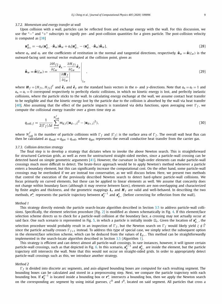
Method 1This strategy directly extends the particle search-locate algorithm described in Section 3.5 to address particle-wall colli-

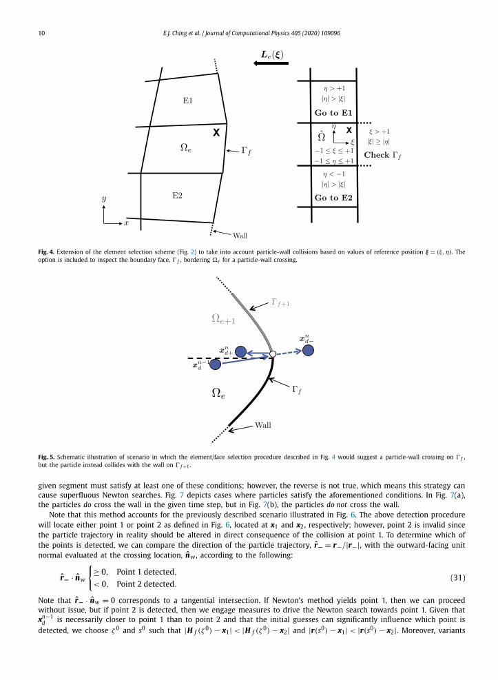
sions. Specifically, the element selection procedure (Fig. 2) is modified as shown schematically in Fig. 4. If this element/face selection scheme directs us to check for a particle-wall collision at the boundary face, a crossing may not actually occur at said face. One such scenario is represented in Fig. 5, in which a particle is initially inside �e . Given the location of xn

d− , the selection procedure would probably result in an inspection of � f , but the Newton search on � f would likely yield ζ /∈ �

since the particle actually crosses � f +1 instead. To address this type of special case, we simply select the subsequent option in the element/face selection scheme, which can be deduced from the values of ξd− . This method can be straightforwardly implemented in the search-locate algorithm described in Section 3.5 (Algorithm 1).

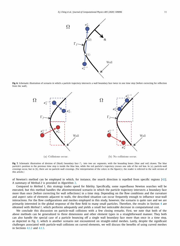
This strategy is efficient and can detect almost all particle-wall crossings. In rare instances, however, it will ignore certain particle-wall crossings, such as that depicted in Fig. 6. In this scenario, xn−1

d and xnd− are inside the element, but the particle

trajectory still intersects the wall. Note that this would not occur on straight-sided grids. In order to appropriately detect particle-wall crossings such as this, we introduce another strategy.

Method 2� f is divided into discrete arc segments, and axis-aligned bounding boxes are computed for each resulting segment. The

bounding boxes can be calculated and stored in a preprocessing step. Next, we compare the particle trajectory with each bounding box. If xn−1

d is located inside a bounding box or rn− intersects a bounding box, then we apply the Newton search on the corresponding arc segment by using initial guesses, ζ 0 and s0, located on said segment. All particles that cross a

10 E.J. Ching et al. / Journal of Computational Physics 405 (2020) 109096

Fig. 4. Extension of the element selection scheme (Fig. 2) to take into account particle-wall collisions based on values of reference position ξ = (ξ, η). The option is included to inspect the boundary face, � f , bordering �e for a particle-wall crossing.

Fig. 5. Schematic illustration of scenario in which the element/face selection procedure described in Fig. 4 would suggest a particle-wall crossing on � f , but the particle instead collides with the wall on � f +1.

given segment must satisfy at least one of these conditions; however, the reverse is not true, which means this strategy can cause superfluous Newton searches. Fig. 7 depicts cases where particles satisfy the aforementioned conditions. In Fig. 7(a), the particles do cross the wall in the given time step, but in Fig. 7(b), the particles do not cross the wall.

Note that this method accounts for the previously described scenario illustrated in Fig. 6. The above detection procedure will locate either point 1 or point 2 as defined in Fig. 6, located at x1 and x2, respectively; however, point 2 is invalid since the particle trajectory in reality should be altered in direct consequence of the collision at point 1. To determine which of the points is detected, we can compare the direction of the particle trajectory, r− = r−/|r−|, with the outward-facing unit normal evaluated at the crossing location, nw , according to the following:

r− · nw

{≥ 0, Point 1 detected,

< 0, Point 2 detected.(31)

Note that r− · nw = 0 corresponds to a tangential intersection. If Newton’s method yields point 1, then we can proceed without issue, but if point 2 is detected, then we engage measures to drive the Newton search towards point 1. Given that xn−1

d is necessarily closer to point 1 than to point 2 and that the initial guesses can significantly influence which point is detected, we choose ζ 0 and s0 such that |H f (ζ

0) − x1| < |H f (ζ0) − x2| and |r(s0) − x1| < |r(s0) − x2|. Moreover, variants

E.J. Ching et al. / Journal of Computational Physics 405 (2020) 109096 11

Fig. 6. Schematic illustration of scenario in which a particle trajectory intersects a wall boundary face twice in one time step (before correcting for reflection from the wall).

Fig. 7. Schematic illustration of division of (black) boundary face � f into two arc segments, with the bounding boxes (blue and red) drawn. The blue particle’s position in the previous time step is inside the blue box, while the red particle’s trajectory crosses one side of the red box. In (a), particle-wall crossings occur, but in (b), there are no particle-wall crossings. (For interpretation of the colors in the figure(s), the reader is referred to the web version of this article.)

of Newton’s method can be employed in which, for instance, the search direction is repelled from specific regions [42]. A summary of Method 2 is provided in Algorithm 2.

Compared to Method 1, this strategy trades speed for fidelity. Specifically, some superfluous Newton searches will be executed, but this method handles the aforementioned scenario in which the particle trajectory intersects a boundary face more than once (before correcting for wall reflections) in a time step. Depending on the flow conditions and the curvature and aspect ratio of elements adjacent to walls, the described situation can occur frequently enough to influence near-wall interactions. For the flow configurations and meshes employed in this study, however, the scenario is quite rare and we are primarily interested in the global response of the flow field to many small particles. Therefore, the results in Section 4 are obtained with Method 1, which performs adequately and yields a small but noticeable decrease in computational cost.

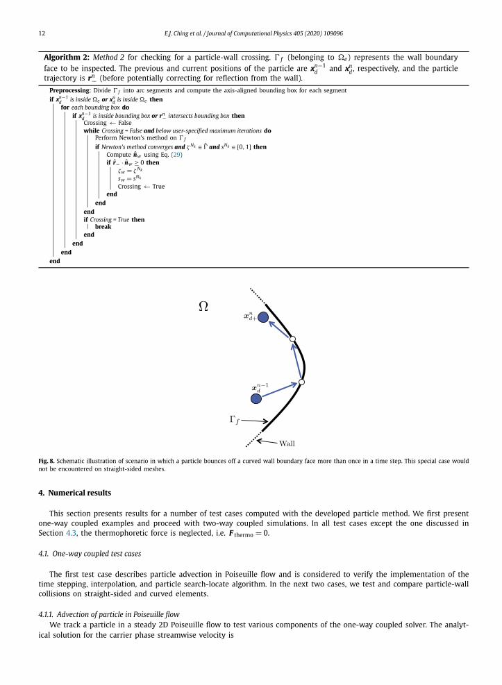
We conclude this discussion on particle-wall collisions with a few closing remarks. First, we note that both of the above methods can be generalized to three dimensions and other element types in a straightforward manner. They both can also handle the special case of a particle bouncing off a single wall boundary face more than once in a time step, as depicted in Fig. 8, which is another scenario not encountered on straight-sided meshes. Lastly, despite the significant challenges associated with particle-wall collisions on curved elements, we will discuss the benefits of using curved meshes in Sections 4.1.2 and 4.1.3.

12 E.J. Ching et al. / Journal of Computational Physics 405 (2020) 109096

Algorithm 2: Method 2 for checking for a particle-wall crossing. � f (belonging to �e) represents the wall boundary face to be inspected. The previous and current positions of the particle are xn−1

d and xnd , respectively, and the particle

trajectory is rn− (before potentially correcting for reflection from the wall).

Preprocessing: Divide � f into arc segments and compute the axis-aligned bounding box for each segment

if xn−1d is inside �e or xn

d is inside �e thenfor each bounding box do

if xn−1d is inside bounding box or rn− intersects bounding box thenCrossing ← Falsewhile Crossing = False and below user-specified maximum iterations do

Perform Newton’s method on � f

if Newton’s method converges and ζ Nk ∈ � and sNk ∈ [0, 1] thenCompute nw using Eq. (29)if r− · nw ≥ 0 then

ζw = ζ Nk

sw = sNk

Crossing ← Trueend

endendif Crossing = True then

breakend

endend

end

Fig. 8. Schematic illustration of scenario in which a particle bounces off a curved wall boundary face more than once in a time step. This special case would not be encountered on straight-sided meshes.

4. Numerical results

This section presents results for a number of test cases computed with the developed particle method. We first present one-way coupled examples and proceed with two-way coupled simulations. In all test cases except the one discussed in Section 4.3, the thermophoretic force is neglected, i.e. F thermo = 0.

4.1. One-way coupled test cases

The first test case describes particle advection in Poiseuille flow and is considered to verify the implementation of the time stepping, interpolation, and particle search-locate algorithm. In the next two cases, we test and compare particle-wall collisions on straight-sided and curved elements.

4.1.1. Advection of particle in Poiseuille flowWe track a particle in a steady 2D Poiseuille flow to test various components of the one-way coupled solver. The analyt-

ical solution for the carrier phase streamwise velocity is

E.J. Ching et al. / Journal of Computational Physics 405 (2020) 109096 13

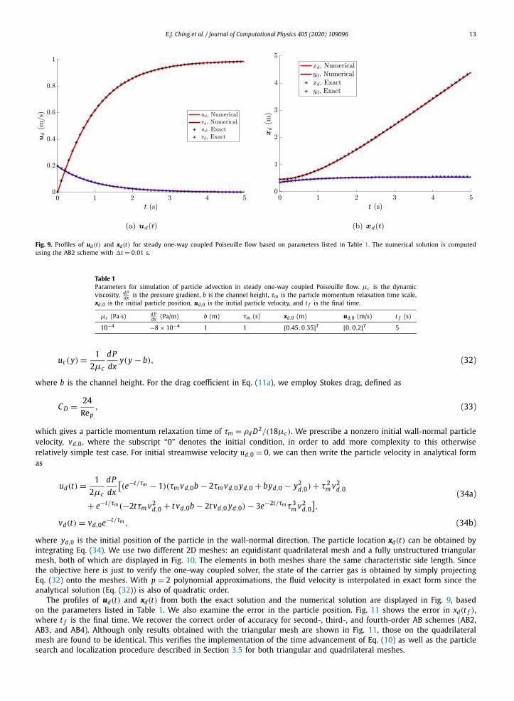
Fig. 9. Profiles of ud(t) and xd(t) for steady one-way coupled Poiseuille flow based on parameters listed in Table 1. The numerical solution is computed using the AB2 scheme with �t = 0.01 s.

Table 1Parameters for simulation of particle advection in steady one-way coupled Poiseuille flow. μc is the dynamic viscosity, dP

dx is the pressure gradient, b is the channel height, τm is the particle momentum relaxation time scale, xd,0 is the initial particle position, ud,0 is the initial particle velocity, and t f is the final time.

μc (Pa·s) dPdx (Pa/m) b (m) τm (s) xd,0 (m) ud,0 (m/s) t f (s)

10−4 −8 × 10−4 1 1 [0.45,0.35]T [0,0.2]T 5

uc(y) = 1

2μc

dP

dxy(y − b), (32)

where b is the channel height. For the drag coefficient in Eq. (11a), we employ Stokes drag, defined as

C D = 24

Rep, (33)

which gives a particle momentum relaxation time of τm = ρd D2/(18μc). We prescribe a nonzero initial wall-normal particle velocity, vd,0, where the subscript “0” denotes the initial condition, in order to add more complexity to this otherwise relatively simple test case. For initial streamwise velocity ud,0 = 0, we can then write the particle velocity in analytical form as

ud(t) = 1

2μc

dP

dx

[(e−t/τm − 1)(τm vd,0b − 2τm vd,0 yd,0 + byd,0 − y2

d,0) + τ 2m v2

d,0

+ e−t/τm (−2tτm v2d,0 + tvd,0b − 2tvd,0 yd,0) − 3e−2t/τmτ 3

m v2d,0

],

(34a)

vd(t) = vd,0e−t/τm , (34b)

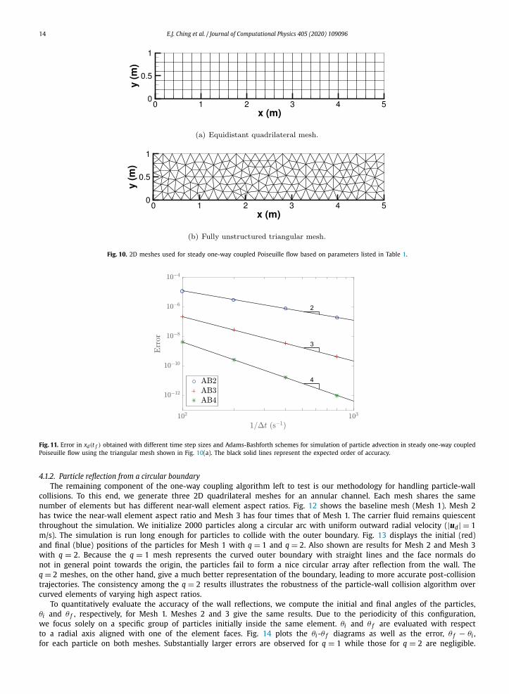
where yd,0 is the initial position of the particle in the wall-normal direction. The particle location xd(t) can be obtained by integrating Eq. (34). We use two different 2D meshes: an equidistant quadrilateral mesh and a fully unstructured triangular mesh, both of which are displayed in Fig. 10. The elements in both meshes share the same characteristic side length. Since the objective here is just to verify the one-way coupled solver, the state of the carrier gas is obtained by simply projecting Eq. (32) onto the meshes. With p = 2 polynomial approximations, the fluid velocity is interpolated in exact form since the analytical solution (Eq. (32)) is also of quadratic order.

The profiles of ud(t) and xd(t) from both the exact solution and the numerical solution are displayed in Fig. 9, based on the parameters listed in Table 1. We also examine the error in the particle position. Fig. 11 shows the error in xd(t f ), where t f is the final time. We recover the correct order of accuracy for second-, third-, and fourth-order AB schemes (AB2, AB3, and AB4). Although only results obtained with the triangular mesh are shown in Fig. 11, those on the quadrilateral mesh are found to be identical. This verifies the implementation of the time advancement of Eq. (10) as well as the particle search and localization procedure described in Section 3.5 for both triangular and quadrilateral meshes.

14 E.J. Ching et al. / Journal of Computational Physics 405 (2020) 109096

Fig. 10. 2D meshes used for steady one-way coupled Poiseuille flow based on parameters listed in Table 1.

Fig. 11. Error in xd(t f ) obtained with different time step sizes and Adams-Bashforth schemes for simulation of particle advection in steady one-way coupled Poiseuille flow using the triangular mesh shown in Fig. 10(a). The black solid lines represent the expected order of accuracy.

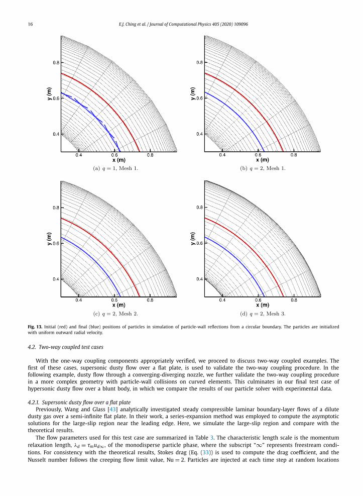
4.1.2. Particle reflection from a circular boundaryThe remaining component of the one-way coupling algorithm left to test is our methodology for handling particle-wall

collisions. To this end, we generate three 2D quadrilateral meshes for an annular channel. Each mesh shares the same number of elements but has different near-wall element aspect ratios. Fig. 12 shows the baseline mesh (Mesh 1). Mesh 2 has twice the near-wall element aspect ratio and Mesh 3 has four times that of Mesh 1. The carrier fluid remains quiescent throughout the simulation. We initialize 2000 particles along a circular arc with uniform outward radial velocity (|ud| = 1m/s). The simulation is run long enough for particles to collide with the outer boundary. Fig. 13 displays the initial (red) and final (blue) positions of the particles for Mesh 1 with q = 1 and q = 2. Also shown are results for Mesh 2 and Mesh 3 with q = 2. Because the q = 1 mesh represents the curved outer boundary with straight lines and the face normals do not in general point towards the origin, the particles fail to form a nice circular array after reflection from the wall. The q = 2 meshes, on the other hand, give a much better representation of the boundary, leading to more accurate post-collision trajectories. The consistency among the q = 2 results illustrates the robustness of the particle-wall collision algorithm over curved elements of varying high aspect ratios.

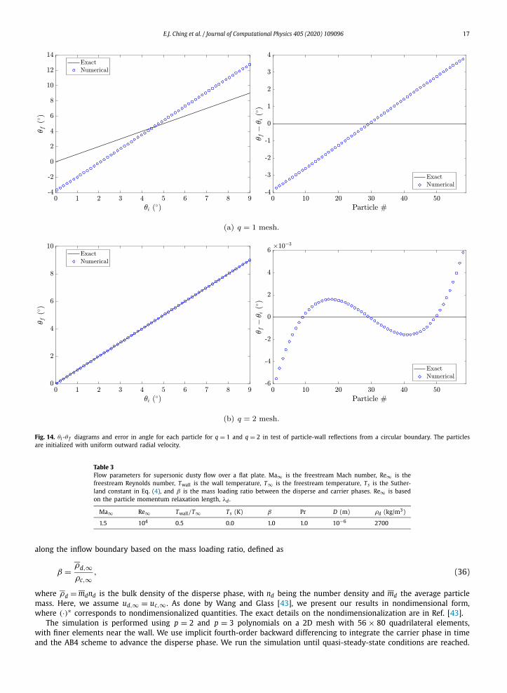
To quantitatively evaluate the accuracy of the wall reflections, we compute the initial and final angles of the particles, θi and θ f , respectively, for Mesh 1. Meshes 2 and 3 give the same results. Due to the periodicity of this configuration, we focus solely on a specific group of particles initially inside the same element. θi and θ f are evaluated with respect to a radial axis aligned with one of the element faces. Fig. 14 plots the θi -θ f diagrams as well as the error, θ f − θi , for each particle on both meshes. Substantially larger errors are observed for q = 1 while those for q = 2 are negligible.

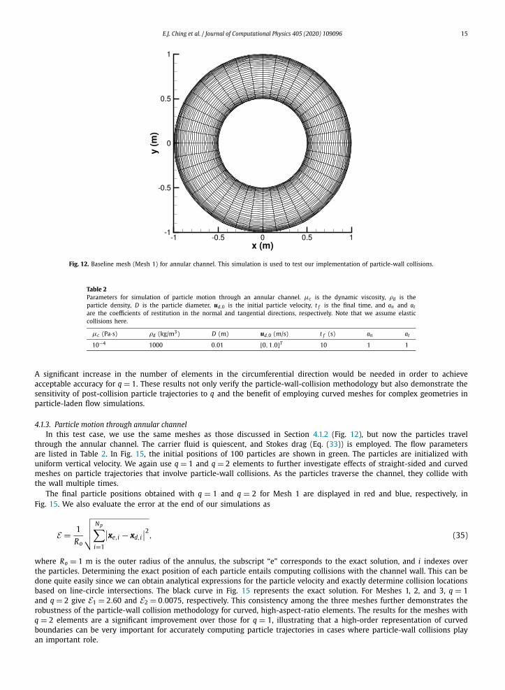
E.J. Ching et al. / Journal of Computational Physics 405 (2020) 109096 15

Fig. 12. Baseline mesh (Mesh 1) for annular channel. This simulation is used to test our implementation of particle-wall collisions.

Table 2Parameters for simulation of particle motion through an annular channel. μc is the dynamic viscosity, ρd is the particle density, D is the particle diameter, ud,0 is the initial particle velocity, t f is the final time, and an and at

are the coefficients of restitution in the normal and tangential directions, respectively. Note that we assume elastic collisions here.

μc (Pa·s) ρd (kg/m3) D (m) ud,0 (m/s) t f (s) an at

10−4 1000 0.01 [0,1.0]T 10 1 1

A significant increase in the number of elements in the circumferential direction would be needed in order to achieve acceptable accuracy for q = 1. These results not only verify the particle-wall-collision methodology but also demonstrate the sensitivity of post-collision particle trajectories to q and the benefit of employing curved meshes for complex geometries in particle-laden flow simulations.

4.1.3. Particle motion through annular channelIn this test case, we use the same meshes as those discussed in Section 4.1.2 (Fig. 12), but now the particles travel

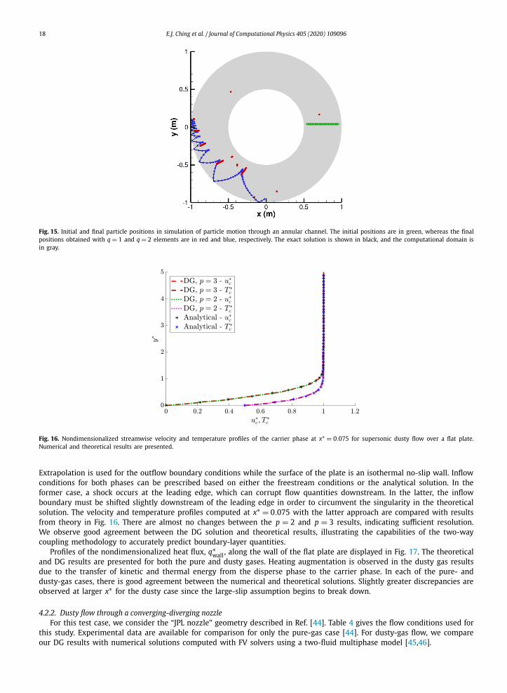
through the annular channel. The carrier fluid is quiescent, and Stokes drag (Eq. (33)) is employed. The flow parameters are listed in Table 2. In Fig. 15, the initial positions of 100 particles are shown in green. The particles are initialized with uniform vertical velocity. We again use q = 1 and q = 2 elements to further investigate effects of straight-sided and curved meshes on particle trajectories that involve particle-wall collisions. As the particles traverse the channel, they collide with the wall multiple times.

The final particle positions obtained with q = 1 and q = 2 for Mesh 1 are displayed in red and blue, respectively, in Fig. 15. We also evaluate the error at the end of our simulations as

E = 1

Ro

√√√√ N p∑i=1

∣∣xe,i − xd,i∣∣2

, (35)

where Ro = 1 m is the outer radius of the annulus, the subscript “e” corresponds to the exact solution, and i indexes over the particles. Determining the exact position of each particle entails computing collisions with the channel wall. This can be done quite easily since we can obtain analytical expressions for the particle velocity and exactly determine collision locations based on line-circle intersections. The black curve in Fig. 15 represents the exact solution. For Meshes 1, 2, and 3, q = 1and q = 2 give E1 = 2.60 and E2 = 0.0075, respectively. This consistency among the three meshes further demonstrates the robustness of the particle-wall collision methodology for curved, high-aspect-ratio elements. The results for the meshes with q = 2 elements are a significant improvement over those for q = 1, illustrating that a high-order representation of curved boundaries can be very important for accurately computing particle trajectories in cases where particle-wall collisions play an important role.

16 E.J. Ching et al. / Journal of Computational Physics 405 (2020) 109096

Fig. 13. Initial (red) and final (blue) positions of particles in simulation of particle-wall reflections from a circular boundary. The particles are initialized with uniform outward radial velocity.

4.2. Two-way coupled test cases

With the one-way coupling components appropriately verified, we proceed to discuss two-way coupled examples. The first of these cases, supersonic dusty flow over a flat plate, is used to validate the two-way coupling procedure. In the following example, dusty flow through a converging-diverging nozzle, we further validate the two-way coupling procedure in a more complex geometry with particle-wall collisions on curved elements. This culminates in our final test case of hypersonic dusty flow over a blunt body, in which we compare the results of our particle solver with experimental data.

4.2.1. Supersonic dusty flow over a flat platePreviously, Wang and Glass [43] analytically investigated steady compressible laminar boundary-layer flows of a dilute

dusty gas over a semi-infinite flat plate. In their work, a series-expansion method was employed to compute the asymptotic solutions for the large-slip region near the leading edge. Here, we simulate the large-slip region and compare with the theoretical results.

The flow parameters used for this test case are summarized in Table 3. The characteristic length scale is the momentum relaxation length, λd = τmud∞ , of the monodisperse particle phase, where the subscript “∞” represents freestream condi-tions. For consistency with the theoretical results, Stokes drag (Eq. (33)) is used to compute the drag coefficient, and the Nusselt number follows the creeping flow limit value, Nu = 2. Particles are injected at each time step at random locations

E.J. Ching et al. / Journal of Computational Physics 405 (2020) 109096 17

Fig. 14. θi -θ f diagrams and error in angle for each particle for q = 1 and q = 2 in test of particle-wall reflections from a circular boundary. The particles are initialized with uniform outward radial velocity.

Table 3Flow parameters for supersonic dusty flow over a flat plate. Ma∞ is the freestream Mach number, Re∞ is the freestream Reynolds number, Twall is the wall temperature, T∞ is the freestream temperature, Ts is the Suther-land constant in Eq. (4), and β is the mass loading ratio between the disperse and carrier phases. Re∞ is based on the particle momentum relaxation length, λd .

Ma∞ Re∞ Twall/T∞ Ts (K) β Pr D (m) ρd (kg/m3)

1.5 104 0.5 0.0 1.0 1.0 10−6 2700

along the inflow boundary based on the mass loading ratio, defined as

β = ρd,∞ρc,∞

, (36)

where ρd = mdnd is the bulk density of the disperse phase, with nd being the number density and md the average particle mass. Here, we assume ud,∞ = uc,∞ . As done by Wang and Glass [43], we present our results in nondimensional form, where (·)∗ corresponds to nondimensionalized quantities. The exact details on the nondimensionalization are in Ref. [43].

The simulation is performed using p = 2 and p = 3 polynomials on a 2D mesh with 56 × 80 quadrilateral elements, with finer elements near the wall. We use implicit fourth-order backward differencing to integrate the carrier phase in time and the AB4 scheme to advance the disperse phase. We run the simulation until quasi-steady-state conditions are reached.

18 E.J. Ching et al. / Journal of Computational Physics 405 (2020) 109096

Fig. 15. Initial and final particle positions in simulation of particle motion through an annular channel. The initial positions are in green, whereas the final positions obtained with q = 1 and q = 2 elements are in red and blue, respectively. The exact solution is shown in black, and the computational domain is in gray.

Fig. 16. Nondimensionalized streamwise velocity and temperature profiles of the carrier phase at x∗ = 0.075 for supersonic dusty flow over a flat plate. Numerical and theoretical results are presented.

Extrapolation is used for the outflow boundary conditions while the surface of the plate is an isothermal no-slip wall. Inflow conditions for both phases can be prescribed based on either the freestream conditions or the analytical solution. In the former case, a shock occurs at the leading edge, which can corrupt flow quantities downstream. In the latter, the inflow boundary must be shifted slightly downstream of the leading edge in order to circumvent the singularity in the theoretical solution. The velocity and temperature profiles computed at x∗ = 0.075 with the latter approach are compared with results from theory in Fig. 16. There are almost no changes between the p = 2 and p = 3 results, indicating sufficient resolution. We observe good agreement between the DG solution and theoretical results, illustrating the capabilities of the two-way coupling methodology to accurately predict boundary-layer quantities.

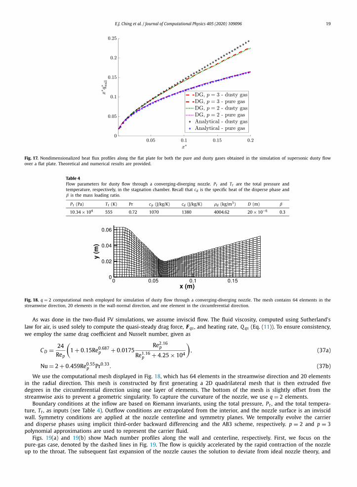
Profiles of the nondimensionalized heat flux, q∗wall , along the wall of the flat plate are displayed in Fig. 17. The theoretical

and DG results are presented for both the pure and dusty gases. Heating augmentation is observed in the dusty gas results due to the transfer of kinetic and thermal energy from the disperse phase to the carrier phase. In each of the pure- and dusty-gas cases, there is good agreement between the numerical and theoretical solutions. Slightly greater discrepancies are observed at larger x∗ for the dusty case since the large-slip assumption begins to break down.

4.2.2. Dusty flow through a converging-diverging nozzleFor this test case, we consider the “JPL nozzle” geometry described in Ref. [44]. Table 4 gives the flow conditions used for

this study. Experimental data are available for comparison for only the pure-gas case [44]. For dusty-gas flow, we compare our DG results with numerical solutions computed with FV solvers using a two-fluid multiphase model [45,46].

E.J. Ching et al. / Journal of Computational Physics 405 (2020) 109096 19

Fig. 17. Nondimensionalized heat flux profiles along the flat plate for both the pure and dusty gases obtained in the simulation of supersonic dusty flow over a flat plate. Theoretical and numerical results are provided.

Table 4Flow parameters for dusty flow through a converging-diverging nozzle. Pt and Tt are the total pressure and temperature, respectively, in the stagnation chamber. Recall that cd is the specific heat of the disperse phase and β is the mass loading ratio.

Pt (Pa) Tt (K) Pr cp (J/kg/K) cd (J/kg/K) ρd (kg/m3) D (m) β

10.34 × 104 555 0.72 1070 1380 4004.62 20 × 10−6 0.3

Fig. 18. q = 2 computational mesh employed for simulation of dusty flow through a converging-diverging nozzle. The mesh contains 64 elements in the streamwise direction, 20 elements in the wall-normal direction, and one element in the circumferential direction.

As was done in the two-fluid FV simulations, we assume inviscid flow. The fluid viscosity, computed using Sutherland’s law for air, is used solely to compute the quasi-steady drag force, F qs , and heating rate, Q qs (Eq. (11)). To ensure consistency, we employ the same drag coefficient and Nusselt number, given as

C D = 24

Rep

(1 + 0.15Re0.687

p + 0.0175Re2.16

p

Re1.16p + 4.25 × 104

), (37a)

Nu = 2 + 0.459Re0.55p Pr0.33. (37b)

We use the computational mesh displayed in Fig. 18, which has 64 elements in the streamwise direction and 20 elements in the radial direction. This mesh is constructed by first generating a 2D quadrilateral mesh that is then extruded five degrees in the circumferential direction using one layer of elements. The bottom of the mesh is slightly offset from the streamwise axis to prevent a geometric singularity. To capture the curvature of the nozzle, we use q = 2 elements.

Boundary conditions at the inflow are based on Riemann invariants, using the total pressure, Pt , and the total tempera-ture, Tt , as inputs (see Table 4). Outflow conditions are extrapolated from the interior, and the nozzle surface is an inviscid wall. Symmetry conditions are applied at the nozzle centerline and symmetry planes. We temporally evolve the carrier and disperse phases using implicit third-order backward differencing and the AB3 scheme, respectively. p = 2 and p = 3polynomial approximations are used to represent the carrier fluid.

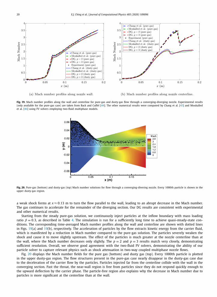
Figs. 19(a) and 19(b) show Mach number profiles along the wall and centerline, respectively. First, we focus on the pure-gas case, denoted by the dashed lines in Fig. 19. The flow is quickly accelerated by the rapid contraction of the nozzle up to the throat. The subsequent fast expansion of the nozzle causes the solution to deviate from ideal nozzle theory, and

20 E.J. Ching et al. / Journal of Computational Physics 405 (2020) 109096

Fig. 19. Mach number profiles along the wall and centerline for pure-gas and dusty-gas flow through a converging-diverging nozzle. Experimental results (only available for the pure-gas case) are taken from Back and Cuffel [44]. The other numerical results were computed by Chang et al. [45] and Moukalled et al. [46] using FV solvers employing two-fluid multiphase models.

Fig. 20. Pure-gas (bottom) and dusty-gas (top) Mach number solutions for flow through a converging-divering nozzle. Every 1000th particle is shown in the upper dusty-gas region.

a weak shock forms at x ≈ 0.13 m to turn the flow parallel to the wall, leading to an abrupt decrease in the Mach number. The gas continues to accelerate for the remainder of the diverging section. Our DG results are consistent with experimental and other numerical results.

Starting from the steady pure-gas solution, we continuously inject particles at the inflow boundary with mass loading ratio β = 0.3, as described in Table 4. The simulation is run for a sufficiently long time to achieve quasi-steady-state con-ditions. The corresponding time-averaged Mach number profiles along the wall and centerline are shown with dotted lines in Figs. 19(a) and 19(b), respectively. The acceleration of particles by the flow extracts kinetic energy from the carrier fluid, which is manifested by a reduction in Mach number compared to the pure-gas solution. The particles severely weaken the shock and cause it to move slightly upstream. The effect of the particles is much greater at the nozzle centerline than at the wall, where the Mach number decreases only slightly. The p = 2 and p = 3 results match very closely, demonstrating sufficient resolution. Overall, we observe good agreement with the two-fluid FV solvers, demonstrating the ability of our particle solver to capture relevant physics such as shock attenuation in two-way coupled multiphase nozzle flows.

Fig. 20 displays the Mach number fields for the pure gas (bottom) and dusty gas (top). Every 1000th particle is plotted in the upper dusty-gas region. The flow structures present in the pure-gas case nearly disappear in the dusty-gas case due to the deceleration of the carrier flow by the particles. Particles injected far from the centerline collide with the wall in the converging section. Past the throat, the near-wall region is free from particles since they do not respond quickly enough to the upward deflection by the carrier phase. The particle-free region also explains why the decrease in Mach number due to particles is more significant at the centerline than at the wall.

E.J. Ching et al. / Journal of Computational Physics 405 (2020) 109096 21

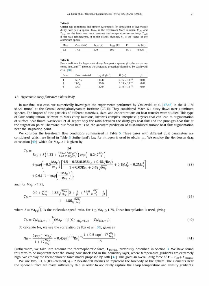
Table 5Carrier gas conditions and sphere parameters for simulation of hypersonic dusty flow past a sphere. Ma∞ is the freestream Mach number, Pt,∞ and Tt,∞ are the freestream total pressure and temperature, respectively, Twallis the wall temperature, Pr is the Prandtl number, Rs is the radius of the aluminum sphere.

Ma∞ Pt,∞ (bar) Tt,∞ (K) Twall (K) Pr Rs (m)

6.1 17.5 570 300 0.71 0.006

Table 6Dust conditions for hypersonic dusty flow past a sphere. β is the mass con-centration, and (·) denotes the averaging procedure described by Vasilevskii et al. [48].

Case Dust material ρd (kg/m3) D (m) β

1 Si3N4 3440 0.16 × 10−6 0.012 SiO2 2264 0.19 × 10−6 0.013 SiO2 2264 0.19 × 10−6 0.04

4.3. Hypersonic dusty flow over a blunt body

In our final test case, we numerically investigate the experiments performed by Vasilevskii et al. [47,48] in the U1-1M shock tunnel at the Central Aerohydrodynamics Institute (CAHI). They considered Mach 6.1 dusty flows over aluminum spheres. The impact of dust particles of different materials, sizes, and concentrations on heat transfer were studied. This type of flow configuration, relevant to Mars entry missions, involves complex interphase physics that can lead to augmentation of surface heat fluxes. Vasilevskii et al. report only the ratio between the dusty-gas heat flux and the pure-gas heat flux at the stagnation point. Therefore, our focus here is on the accurate prediction of dust-induced surface heat flux augmentation near the stagnation point.

We consider the freestream flow conditions summarized in Table 5. Three cases with different dust parameters are considered, which are listed in Table 6. Sutherland’s law for nitrogen is used to obtain μc . We employ the Henderson drag correlation [49], which for Map < 1 is given by

C D = 24

Rep + S(

4.33 + 3.65−1.53Td/Tc1+0.353Td/Tc

)exp

(−0.247 Rep

S

)+ exp

(−0.5

Map

Rep

)[4.5 + 0.38(0.03Rep + 0.48

√Rep)

1 + 0.03Rep + 0.48√

Rep+ 0.1Ma2

p + 0.2Ma8p

](38)

+ 0.6S

[1 − exp

(−Map

Rep

)],

and, for Map > 1.75,

C D =0.9 + 0.34

Map+ 1.86

√MapRep

[2 + 2

S2 + 1.058S

√TdTc

− 1S4

]1 + 1.86

√MapRep

, (39)

where S = Map

√γ2 is the molecular speed ratio. For 1 ≤ Map ≤ 1.75, linear interpolation is used, giving

C D = C D |Map=1 + 4

3(Map − 1)( C D |Map=1.75 − C D |Map=1). (40)

To calculate Nu, we use the correlation by Fox et al. [50], given as

Nu = 2 exp(−Map)

1 + 17 MapRep

+ 0.459Pr0.33Re0.55p

1 + 0.5 exp(−17 MapRep

)

1.5. (41)

Furthermore, we take into account the thermophoretic force, F thermo, previously described in Section 3. We have found this term to be important near the strong bow shock and in the boundary layer, where temperature gradients are extremely high. We employ the themophoretic force model proposed by Loth [37]. This gives an overall drag force of F = F qs + F thermo.

We use two 3D, 60,000-element, q = 2 hexahedral meshes to represent the forebody of the sphere. The elements near the sphere surface are made sufficiently thin in order to accurately capture the sharp temperature and density gradients.

22 E.J. Ching et al. / Journal of Computational Physics 405 (2020) 109096

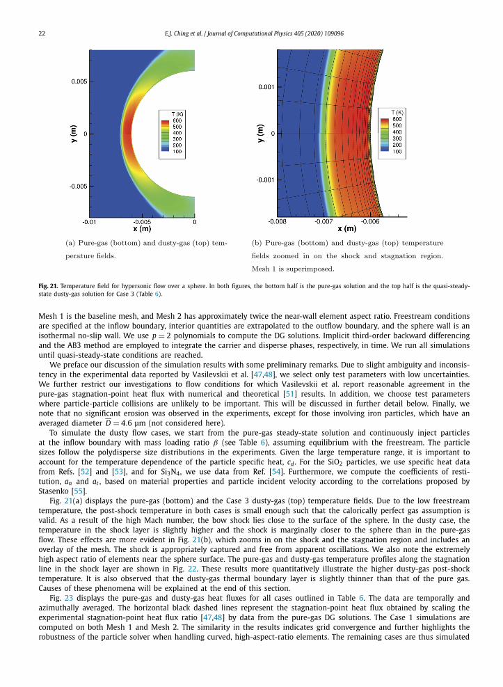
Fig. 21. Temperature field for hypersonic flow over a sphere. In both figures, the bottom half is the pure-gas solution and the top half is the quasi-steady-state dusty-gas solution for Case 3 (Table 6).

Mesh 1 is the baseline mesh, and Mesh 2 has approximately twice the near-wall element aspect ratio. Freestream conditions are specified at the inflow boundary, interior quantities are extrapolated to the outflow boundary, and the sphere wall is an isothermal no-slip wall. We use p = 2 polynomials to compute the DG solutions. Implicit third-order backward differencing and the AB3 method are employed to integrate the carrier and disperse phases, respectively, in time. We run all simulations until quasi-steady-state conditions are reached.

We preface our discussion of the simulation results with some preliminary remarks. Due to slight ambiguity and inconsis-tency in the experimental data reported by Vasilevskii et al. [47,48], we select only test parameters with low uncertainties. We further restrict our investigations to flow conditions for which Vasilevskii et al. report reasonable agreement in the pure-gas stagnation-point heat flux with numerical and theoretical [51] results. In addition, we choose test parameters where particle-particle collisions are unlikely to be important. This will be discussed in further detail below. Finally, we note that no significant erosion was observed in the experiments, except for those involving iron particles, which have an averaged diameter D = 4.6 μm (not considered here).

To simulate the dusty flow cases, we start from the pure-gas steady-state solution and continuously inject particles at the inflow boundary with mass loading ratio β (see Table 6), assuming equilibrium with the freestream. The particle sizes follow the polydisperse size distributions in the experiments. Given the large temperature range, it is important to account for the temperature dependence of the particle specific heat, cd . For the SiO2 particles, we use specific heat data from Refs. [52] and [53], and for Si3N4, we use data from Ref. [54]. Furthermore, we compute the coefficients of resti-tution, an and at , based on material properties and particle incident velocity according to the correlations proposed by Stasenko [55].

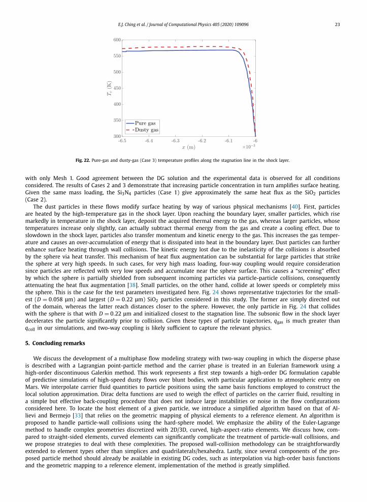
Fig. 21(a) displays the pure-gas (bottom) and the Case 3 dusty-gas (top) temperature fields. Due to the low freestream temperature, the post-shock temperature in both cases is small enough such that the calorically perfect gas assumption is valid. As a result of the high Mach number, the bow shock lies close to the surface of the sphere. In the dusty case, the temperature in the shock layer is slightly higher and the shock is marginally closer to the sphere than in the pure-gas flow. These effects are more evident in Fig. 21(b), which zooms in on the shock and the stagnation region and includes an overlay of the mesh. The shock is appropriately captured and free from apparent oscillations. We also note the extremely high aspect ratio of elements near the sphere surface. The pure-gas and dusty-gas temperature profiles along the stagnation line in the shock layer are shown in Fig. 22. These results more quantitatively illustrate the higher dusty-gas post-shock temperature. It is also observed that the dusty-gas thermal boundary layer is slightly thinner than that of the pure gas. Causes of these phenomena will be explained at the end of this section.

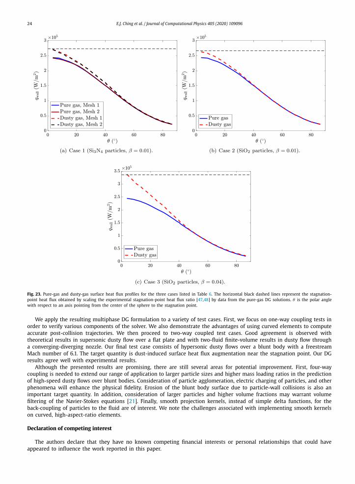
Fig. 23 displays the pure-gas and dusty-gas heat fluxes for all cases outlined in Table 6. The data are temporally and azimuthally averaged. The horizontal black dashed lines represent the stagnation-point heat flux obtained by scaling the experimental stagnation-point heat flux ratio [47,48] by data from the pure-gas DG solutions. The Case 1 simulations are computed on both Mesh 1 and Mesh 2. The similarity in the results indicates grid convergence and further highlights the robustness of the particle solver when handling curved, high-aspect-ratio elements. The remaining cases are thus simulated

E.J. Ching et al. / Journal of Computational Physics 405 (2020) 109096 23

Fig. 22. Pure-gas and dusty-gas (Case 3) temperature profiles along the stagnation line in the shock layer.

with only Mesh 1. Good agreement between the DG solution and the experimental data is observed for all conditions considered. The results of Cases 2 and 3 demonstrate that increasing particle concentration in turn amplifies surface heating. Given the same mass loading, the Si3N4 particles (Case 1) give approximately the same heat flux as the SiO2 particles (Case 2).

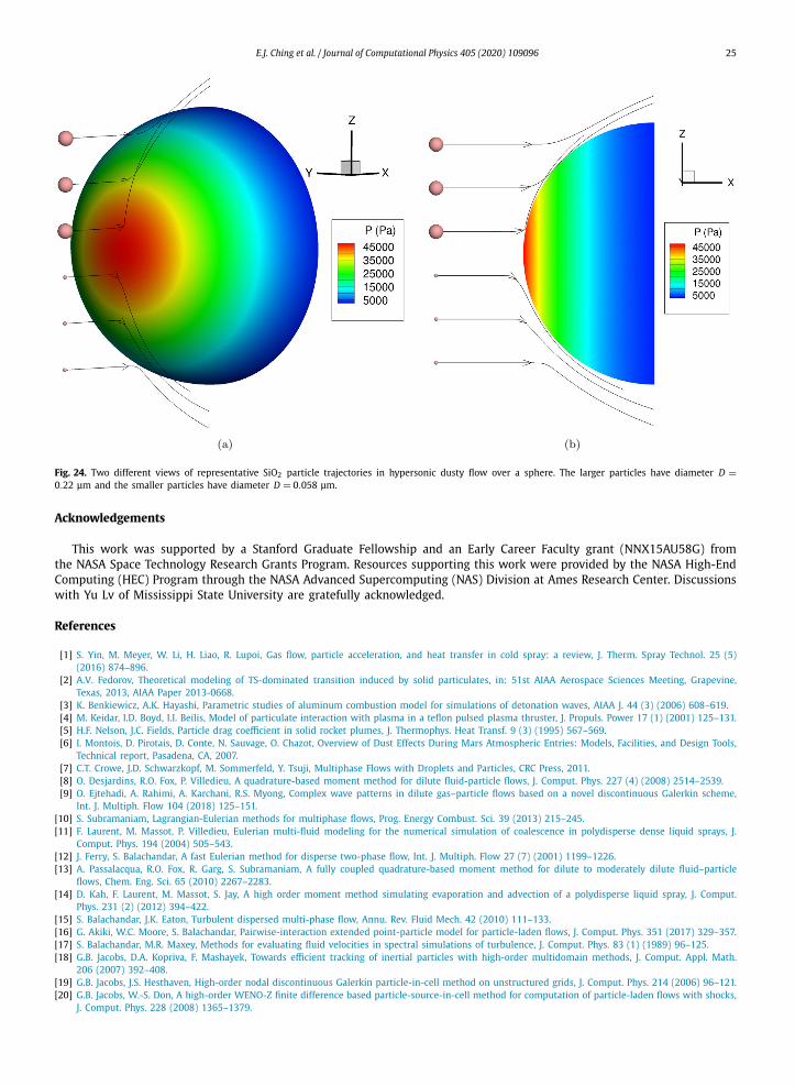
The dust particles in these flows modify surface heating by way of various physical mechanisms [40]. First, particles are heated by the high-temperature gas in the shock layer. Upon reaching the boundary layer, smaller particles, which rise markedly in temperature in the shock layer, deposit the acquired thermal energy to the gas, whereas larger particles, whose temperatures increase only slightly, can actually subtract thermal energy from the gas and create a cooling effect. Due to slowdown in the shock layer, particles also transfer momentum and kinetic energy to the gas. This increases the gas temper-ature and causes an over-accumulation of energy that is dissipated into heat in the boundary layer. Dust particles can further enhance surface heating through wall collisions. The kinetic energy lost due to the inelasticity of the collisions is absorbed by the sphere via heat transfer. This mechanism of heat flux augmentation can be substantial for large particles that strike the sphere at very high speeds. In such cases, for very high mass loading, four-way coupling would require consideration since particles are reflected with very low speeds and accumulate near the sphere surface. This causes a “screening” effect by which the sphere is partially shielded from subsequent incoming particles via particle-particle collisions, consequently attenuating the heat flux augmentation [38]. Small particles, on the other hand, collide at lower speeds or completely miss the sphere. This is the case for the test parameters investigated here. Fig. 24 shows representative trajectories for the small-est (D = 0.058 μm) and largest (D = 0.22 μm) SiO2 particles considered in this study. The former are simply directed out of the domain, whereas the latter reach distances closer to the sphere. However, the only particle in Fig. 24 that collides with the sphere is that with D = 0.22 μm and initialized closest to the stagnation line. The subsonic flow in the shock layer decelerates the particle significantly prior to collision. Given these types of particle trajectories, qgas is much greater than qcoll in our simulations, and two-way coupling is likely sufficient to capture the relevant physics.

5. Concluding remarks

We discuss the development of a multiphase flow modeling strategy with two-way coupling in which the disperse phase is described with a Lagrangian point-particle method and the carrier phase is treated in an Eulerian framework using a high-order discontinuous Galerkin method. This work represents a first step towards a high-order DG formulation capable of predictive simulations of high-speed dusty flows over blunt bodies, with particular application to atmospheric entry on Mars. We interpolate carrier fluid quantities to particle positions using the same basis functions employed to construct the local solution approximation. Dirac delta functions are used to weigh the effect of particles on the carrier fluid, resulting in a simple but effective back-coupling procedure that does not induce large instabilities or noise in the flow configurations considered here. To locate the host element of a given particle, we introduce a simplified algorithm based on that of Al-lievi and Bermejo [33] that relies on the geometric mapping of physical elements to a reference element. An algorithm is proposed to handle particle-wall collisions using the hard-sphere model. We emphasize the ability of the Euler-Lagrange method to handle complex geometries discretized with 2D/3D, curved, high-aspect-ratio elements. We discuss how, com-pared to straight-sided elements, curved elements can significantly complicate the treatment of particle-wall collisions, and we propose strategies to deal with these complexities. The proposed wall-collision methodology can be straightforwardly extended to element types other than simplices and quadrilaterals/hexahedra. Lastly, since several components of the pro-posed particle method should already be available in existing DG codes, such as interpolation via high-order basis functions and the geometric mapping to a reference element, implementation of the method is greatly simplified.

24 E.J. Ching et al. / Journal of Computational Physics 405 (2020) 109096

Fig. 23. Pure-gas and dusty-gas surface heat flux profiles for the three cases listed in Table 6. The horizontal black dashed lines represent the stagnation-point heat flux obtained by scaling the experimental stagnation-point heat flux ratio [47,48] by data from the pure-gas DG solutions. θ is the polar angle with respect to an axis pointing from the center of the sphere to the stagnation point.

We apply the resulting multiphase DG formulation to a variety of test cases. First, we focus on one-way coupling tests in order to verify various components of the solver. We also demonstrate the advantages of using curved elements to compute accurate post-collision trajectories. We then proceed to two-way coupled test cases. Good agreement is observed with theoretical results in supersonic dusty flow over a flat plate and with two-fluid finite-volume results in dusty flow through a converging-diverging nozzle. Our final test case consists of hypersonic dusty flows over a blunt body with a freestream Mach number of 6.1. The target quantity is dust-induced surface heat flux augmentation near the stagnation point. Our DG results agree well with experimental results.

Although the presented results are promising, there are still several areas for potential improvement. First, four-way coupling is needed to extend our range of application to larger particle sizes and higher mass loading ratios in the prediction of high-speed dusty flows over blunt bodies. Consideration of particle agglomeration, electric charging of particles, and other phenomena will enhance the physical fidelity. Erosion of the blunt body surface due to particle-wall collisions is also an important target quantity. In addition, consideration of larger particles and higher volume fractions may warrant volume filtering of the Navier-Stokes equations [21]. Finally, smooth projection kernels, instead of simple delta functions, for the back-coupling of particles to the fluid are of interest. We note the challenges associated with implementing smooth kernels on curved, high-aspect-ratio elements.

Declaration of competing interest

The authors declare that they have no known competing financial interests or personal relationships that could have appeared to influence the work reported in this paper.

E.J. Ching et al. / Journal of Computational Physics 405 (2020) 109096 25

Fig. 24. Two different views of representative SiO2 particle trajectories in hypersonic dusty flow over a sphere. The larger particles have diameter D =0.22 μm and the smaller particles have diameter D = 0.058 μm.

Acknowledgements

This work was supported by a Stanford Graduate Fellowship and an Early Career Faculty grant (NNX15AU58G) from the NASA Space Technology Research Grants Program. Resources supporting this work were provided by the NASA High-End Computing (HEC) Program through the NASA Advanced Supercomputing (NAS) Division at Ames Research Center. Discussions with Yu Lv of Mississippi State University are gratefully acknowledged.

References

[1] S. Yin, M. Meyer, W. Li, H. Liao, R. Lupoi, Gas flow, particle acceleration, and heat transfer in cold spray: a review, J. Therm. Spray Technol. 25 (5) (2016) 874–896.

[2] A.V. Fedorov, Theoretical modeling of TS-dominated transition induced by solid particulates, in: 51st AIAA Aerospace Sciences Meeting, Grapevine, Texas, 2013, AIAA Paper 2013-0668.

[3] K. Benkiewicz, A.K. Hayashi, Parametric studies of aluminum combustion model for simulations of detonation waves, AIAA J. 44 (3) (2006) 608–619.[4] M. Keidar, I.D. Boyd, I.I. Beilis, Model of particulate interaction with plasma in a teflon pulsed plasma thruster, J. Propuls. Power 17 (1) (2001) 125–131.[5] H.F. Nelson, J.C. Fields, Particle drag coefficient in solid rocket plumes, J. Thermophys. Heat Transf. 9 (3) (1995) 567–569.[6] I. Montois, D. Pirotais, D. Conte, N. Sauvage, O. Chazot, Overview of Dust Effects During Mars Atmospheric Entries: Models, Facilities, and Design Tools,

Technical report, Pasadena, CA, 2007.[7] C.T. Crowe, J.D. Schwarzkopf, M. Sommerfeld, Y. Tsuji, Multiphase Flows with Droplets and Particles, CRC Press, 2011.[8] O. Desjardins, R.O. Fox, P. Villedieu, A quadrature-based moment method for dilute fluid-particle flows, J. Comput. Phys. 227 (4) (2008) 2514–2539.[9] O. Ejtehadi, A. Rahimi, A. Karchani, R.S. Myong, Complex wave patterns in dilute gas–particle flows based on a novel discontinuous Galerkin scheme,

Int. J. Multiph. Flow 104 (2018) 125–151.[10] S. Subramaniam, Lagrangian-Eulerian methods for multiphase flows, Prog. Energy Combust. Sci. 39 (2013) 215–245.[11] F. Laurent, M. Massot, P. Villedieu, Eulerian multi-fluid modeling for the numerical simulation of coalescence in polydisperse dense liquid sprays, J.

Comput. Phys. 194 (2004) 505–543.[12] J. Ferry, S. Balachandar, A fast Eulerian method for disperse two-phase flow, Int. J. Multiph. Flow 27 (7) (2001) 1199–1226.[13] A. Passalacqua, R.O. Fox, R. Garg, S. Subramaniam, A fully coupled quadrature-based moment method for dilute to moderately dilute fluid–particle

flows, Chem. Eng. Sci. 65 (2010) 2267–2283.[14] D. Kah, F. Laurent, M. Massot, S. Jay, A high order moment method simulating evaporation and advection of a polydisperse liquid spray, J. Comput.

Phys. 231 (2) (2012) 394–422.[15] S. Balachandar, J.K. Eaton, Turbulent dispersed multi-phase flow, Annu. Rev. Fluid Mech. 42 (2010) 111–133.[16] G. Akiki, W.C. Moore, S. Balachandar, Pairwise-interaction extended point-particle model for particle-laden flows, J. Comput. Phys. 351 (2017) 329–357.[17] S. Balachandar, M.R. Maxey, Methods for evaluating fluid velocities in spectral simulations of turbulence, J. Comput. Phys. 83 (1) (1989) 96–125.[18] G.B. Jacobs, D.A. Kopriva, F. Mashayek, Towards efficient tracking of inertial particles with high-order multidomain methods, J. Comput. Appl. Math.

206 (2007) 392–408.[19] G.B. Jacobs, J.S. Hesthaven, High-order nodal discontinuous Galerkin particle-in-cell method on unstructured grids, J. Comput. Phys. 214 (2006) 96–121.[20] G.B. Jacobs, W.-S. Don, A high-order WENO-Z finite difference based particle-source-in-cell method for computation of particle-laden flows with shocks,

J. Comput. Phys. 228 (2008) 1365–1379.

26 E.J. Ching et al. / Journal of Computational Physics 405 (2020) 109096

[21] J. Capecelatro, O. Desjardins, An Euler-Lagrange strategy for simulating particle-laden flows, J. Comput. Phys. 238 (2013) 1–31.[22] H.P. Zhu, Z.Y. Zhou, R.Y. Yang, A.B. Yu, Discrete particle simulation of particulate systems: theoretical developments, Chem. Eng. Sci. 62 (2007)

3378–3396.[23] S. Sundaram, L.R. Collins, Numerical considerations in simulating a turbulent suspension of finite-volume particles, J. Comput. Phys. 124 (1996)

337–350.[24] K. Sengupta, B. Shotorban, G.B. Jacobs, F. Mashayek, Spectral-based simulations of particle-laden turbulent flows, Int. J. Multiph. Flow 35 (2009)

811–826.[25] Y. Lv, M. Ihme, Discontinuous Galerkin method for multicomponent chemically reacting flows and combustion, J. Comput. Phys. 270 (2014) 105–137.[26] F.Q. Hu, M.Y. Hussaini, P. Rasetarinera, An analysis of the discontinuous Galerkin method for wave propagation problems, J. Comput. Phys. 151 (1999)

2560–2579.[27] M. Sabat, A. Larat, A. Vié, M. Massot, On the development of high order realizable schemes for the Eulerian simulation of disperse phase flows: a

convex-state preserving discontinuous Galerkin method, J. Comput. Multiph. Flows 6 (3) (2014) 247–270.[28] T. Banerjee, J. Hackl, M. Shringarpure, T. Islam, S. Balachandar, T. Jackson, S. Ranka, A new proxy application for compressible multiphase turbulent

flows, Sustain. Comput. Informatics Syst. 16 (2017) 11–24.[29] G.B. Jacobs, J.S. Hesthaven, Implicit–explicit time integration of a high-order particle-in-cell method with hyperbolic divergence cleaning, Comput. Phys.

Commun. 180 (10) (2009) 1760–1767.[30] J. Neudorfer, T. Stindl, A. Stock, R. Schneider, D. Petkow, S. Roller, C.-D. Munz, M. Auweter-Kurtz, Three-dimensional simulation of rarefied plasma flows

using a high order particle in cell method, in: High Performance Computing in Science and Engineering ’10, Springer, 2011, pp. 593–604.[31] T. Stindl, J. Neudorfer, A. Stock, M. Auweter-Kurtz, C.-D. Munz, S. Roller, R. Schneider, Comparison of coupling techniques in a high-order discontinuous

Galerkin-based particle-in-cell solver, J. Phys. D, Appl. Phys. 44 (19) (2011) 194004.[32] A. Stock, J. Neudorfer, M. Riedlinger, G. Pirrung, G. Gassner, R. Schneider, S. Roller, C.-D. Munz, Three-dimensional numerical simulation of a 30-GHz

gyrotron resonator with an explicit high-order discontinuous-Galerkin-based parallel particle-in-cell method, IEEE Trans. Plasma Sci. 40 (7) (2012) 1860–1870.

[33] A. Allievi, R. Bermejo, A generalized particle search-locate algorithm for arbitrary grids, J. Comput. Phys. 132 (1997) 157–166.[34] E.J. Ching, Y. Lv, P. Gnoffo, M. Barnhardt, M. Ihme, Shock capturing for discontinuous Galerkin methods with application to predicting heat transfer in

hypersonic flows, J. Comput. Phys. 376 (2019) 54–75.[35] P.L. Roe, Approximate Riemann solvers, parameter vectors, and difference schemes, J. Comput. Phys. 43 (2) (1981) 357–372.[36] F. Bassi, S. Rebay, GMRES discontinuous Galerkin solution of the compressible Navier-Stokes equations, in: B. Cockburn, C.-W. Shu (Eds.), Discontinuous

Galerkin Methods: Theory, Computation and Applications, Springer, Berlin, 2000, pp. 197–208.[37] E. Loth, Compressibility and rarefaction effects on drag of a spherical particle, AIAA J. 46 (9) (2008) 2219–2228.[38] A.N. Volkov, Y.M. Tsirkunov, Effect of a dispersed admixture on the flow pattern and heat transfer in a supersonic dusty-gas flow around a cylinder,

Fluid Dyn. 40 (4) (2005) 561–574.[39] Y. Ling, S. Balachandar, M. Parmar, Inter-phase heat transfer and energy coupling in turbulent dispersed multiphase flows, Phys. Fluids 28 (3) (2016)

033304.[40] B. Oesterle, A.N. Volkov, Y.M. Tsirkunov, Numerical investigation of two-phase flow structure and heat transfer in a supersonic dusty gas flow over a

blunt body, in: Progress in Flight Physics, vol. 5, 2013, pp. 441–456.[41] R. Chorda, J.A. Blasco, N. Fueyo, An efficient particle-locating algorithm for application in arbitrary 2D and 3D grids, Int. J. Multiph. Flow 28 (9) (2002)

1565–1580.[42] M. Ceze, K.J. Fidkowski, Constrained pseudo-transient continuation, Int. J. Numer. Methods Eng. 102 (11) (2015) 1683–1703.[43] B.Y. Wang, I.I. Glass, Compressible laminar boundary-layer flows of a dusty gas over a semi-infinite flat plate, J. Fluid Mech. 186 (1988) 223–241.[44] L.H. Back, R.F. Cuffel, Detection of oblique shocks in a conical nozzle with a circular-arc throat, AIAA J. 4 (12) (1966) 2219–2221.[45] H.T. Chang, L.W. Hourng, L.C. Chien, Application of flux-vector-splitting scheme to a dilute gas–particle JPL nozzle flow, Int. J. Numer. Methods Fluids

22 (10) (1996) 921–935.[46] F. Moukalled, M. Darwish, B. Sekar, A pressure-based algorithm for multi-phase flow at all speeds, J. Comput. Phys. 190 (2) (2003) 550–571.[47] E. Vasilevskii, A. Osiptsov, Experimental and numerical study of heat transfer on a blunt body in dusty hypersonic flow, in: 33rd AIAA Thermophysics

Conference, Norfolk, Virginia, 1999, AIAA Paper 1999-3563.[48] E.B. Vasilevskii, A.N. Osiptsov, A.V. Chirikhin, L.V. Yakovleva, Heat exchange on the front surface of a blunt body in a high-speed flow containing

low-inertia particles, J. Eng. Phys. Thermophys. 74 (6) (2001) 1399–1411.[49] C.B. Henderson, Drag coefficients of spheres in continuum and rarefied flows, AIAA J. 14 (6) (1976) 707–708.[50] T.W. Fox, C.W. Rackett, J.A. Nicholls, Shock wave ignition of magnesium powers, in: 11th International Shock Tubes and Waves Symposium, Seattle,

Washington, 1978, pp. 262–268.[51] J.A. Fay, Theory of stagnation point heat transfer in dissociated air, J. Aerosp. Sci. 25 (2) (1958) 73–85.[52] Y.S. Touloukian, E.H. Buyco, Thermophysical Properties of Matter - The TPRC Data Series, vol. 5. Specific Heat-Nonmetallic Solids, Technical report,

Thermophysical and Electronic Properties Information Analysis Center, Lafayette, IN, 1970.[53] M.W. Chase Jr., NIST-JANAF Thermochemical Tables, fourth edition, J. Phys. Chem. Ref. Data Monogr., vol. 9, 1998.[54] R.J. Bruls, H.T. Hintzen, G. de With, R. Metselaar, J.C. van Miltenburg, The temperature dependence of the Grüneisen parameters of MgSiN2, AlN and

β-Si3N4, J. Phys. Chem. Solids 62 (4) (2001) 783–792.[55] A.L. Stasenko, Velocity recovery factors of a particle repelled from a solid surface, J. Eng. Phys. Thermophys. 80 (5) (2007) 885–891.