Journal of Computational Physics 228 (2009) 3433–3447

Contents lists available at ScienceDirect

Journal of Computational Physics

journal homepage: www.elsevier .com/locate / jcp

On the accuracy of the rotation form in simulations of the Navier–Stokesequations

William Layton a,*,1, Carolina C. Manica b, Monika Neda c, Maxim Olshanskii d,2, Leo G. Rebholz e

a Department of Mathematics, University of Pittsburgh, United Statesb Departamento de Matemática Pura e Aplicada, Universidade Federal do Rio Grande do Sul, Brazilc Department of Mathematical Sciences, University of Nevada, Las Vegas, United Statesd Department of Mechanics and Mathematics, Moscow State M. V. Lomonosov University, Moscow 119899, Russiae Department of Mathematical Sciences, Clemson University, United States

a r t i c l e i n f o a b s t r a c t

Article history:Received 26 June 2008Received in revised form 9 December 2008Accepted 25 January 2009Available online 6 February 2009

Keywords:Navier–Stokes equationRotation formFinite element method

0021-9991/$ - see front matter � 2009 Elsevier Incdoi:10.1016/j.jcp.2009.01.027

* Corresponding author. Tel.: +1 412 624 8312.E-mail addresses: wjl@pitt.edu (W. Layton), caro

(M. Olshanskii), rebholz@clemson.edu (L.G. RebholzURLs: http://www.math.pitt.edu/~wjl (W. Layt

(M. Neda), http://www.mathcs.emory.edu/~molshan1 Partially supported by NSF Grant DMS 0508260.2 Partially supported by the RAS program ‘‘Contem

01-00415.

The rotation form of the Navier–Stokes equations nonlinearity is commonly used in highReynolds number flow simulations. It was pointed out by a few authors (and not widelyknown apparently) that it can also lead to a less accurate approximate solution than theusual u � ru form. We give a different explanation of this effect related to (i) resolutionof the Bernoulli pressure, and (ii) the scaling of the coupling between velocity and pressureerror with respect to the Reynolds number. We show analytically that (i) the differencebetween the two nonlinearities is governed by the difference in the resolution of the Ber-noulli and kinematic pressures, and (ii) a simple, linear grad–div stabilization amelioratesmuch of the bad scaling of the velocity error with respect to Re. The rotation form doeshave superior conservation properties to the alternatives and it appears to be amenableto more efficient preconditioners. Thus, the rotational form with grad–div stabilization isa promising method. We also give experiments that show bad velocity approximation istied to poor pressure resolution in either form.

� 2009 Elsevier Inc. All rights reserved.

1. Introduction

The nonlinearity in the Navier–Stokes equations (NSE) can be written in several ways, which, while equivalent for thecontinuous NSE, lead to discretizations with different algorithmic costs, conserved quantities, and approximation accuracy,e.g. [9,10]. These forms include the convective form, the skew-symmetric form and the rotation form, given respectively by

u � ru; u � ruþ 12ðdivuÞu; and ðr � uÞ � u:

In turbulent flow simulations, different forms of the nonlinearity are used for different reasons. The algorithmic advantagesand superior conservation properties of the rotation form (summarized in Section 2.2) have led to it being a very common

. All rights reserved.

lina.manica@ufrgs.br (C.C. Manica), Monika.Neda@unlv.edu (M. Neda), Maxim.Olshanskii@mtu-net.ru).on), http://www.chasqueweb.ufrgs.br/~carolina.manica (C.C. Manica), http://faculty.unlv.edu/neda

(M. Olshanskii), http://www.math.pitt.edu/~ler6 (L.G. Rebholz).

porary problems of theoretical mathematics” through the Project No. 01.2.00104588 and RFBR Grant 08-

3434 W. Layton et al. / Journal of Computational Physics 228 (2009) 3433–3447

choice, see, e.g. Chapter 7 in [5,6,24]. Herein we reveal potential limitations of rotation form, and suggest a way to overcomethem.

It is known from Horiuti [14], Horiuti and Itami [15] and Zang [33] that the rotation form can lead to a less accurateapproximate solution when discretized by commonly used numerical methods. Horiuti [14] and Zang [33] each give numer-ical experiments and accompanying analytic arguments suggesting that the accuracy loss may happen due, respectively, todiscretization errors in the near wall regions (Horiuti, for finite-difference methods) and to greater aliasing errors (Zang, forspectral methods). We have noticed the same loss of accuracy in experiments from [20,26] (for finite element methods) andsuggest herein a third possibility that it is due to a combination of:

1. The Bernoulli or dynamic pressure P ¼ pþ 12 juj

2 is generically much more complex than the pressure p, and thus2. Meshes upon which p is fully resolved are typically under resolved for P, and3. As the Reynolds number increases, the discrete momentum equation with either form of the nonlinearity magnifies the

pressure error’s effect upon the velocity error.

We will see, for example, that in the usual formulation Velocity Error � Re* Pressure Error, (2.13). Thus, interestingly, someof the loss of accuracy, although triggered by the nonlinear term, is due to connections between variables already present inthe linear Stokes problem.

In finite element methods (FEM) the inf–sup condition for stability of the pressure places a strong condition linking veloc-ity and pressure degrees of freedom. This condition, while quite technical when precisely stated, roughly implies that forlower order approximations the pressure degrees of freedom should correspond to the velocity degrees of freedom on amesh one step coarser than the velocity mesh, while for higher order finite elements the polynomial degree of pressureapproximations is less than the polynomial degree of velocity approximations. Thus, in either case for velocities u and Ber-noulli pressures P with the same complex structures, as the mesh is refined the velocity will be often fully resolved before theBernoulli pressure is well-resolved, see the experiments in Section 3.3 involving flow around a cylinder. Further, when anartificial problem, constructed so the kinematic pressure and Bernoulli pressure reverse complexity, is solved the observederror behavior is reversed: the convective form has much greater error than the rotation form, Section 3.2.

The question of resolution is reminiscent of Horiuti’s argument based on truncation errors in boundary layers. For exam-ple, even for a simple Prandtl-type, laminar boundary layer, the pressure p will be approximately constant in the near wallregion while the Bernoulli pressure P ¼ pþ 1=2juj2 will share the OðRe�1=2Þ boundary layer of the velocity field.

Point 3 is possibly related to aliasing errors; interestingly, the aliasing error in using different forms of the nonlinearity isgoverned by the resolution of the (Bernoulli or kinematic) pressure. Our suggestion of a ‘‘fix” of using grad–div stabilization(see Section 2.3) works in our tests because it addresses point 3 without requiring extra resolution.

Stabilization of grad–div type reduces the error in divuh, see (2.15), and its (bad) scaling with respect to the Reynoldsnumber. Moreover, since when divuh ¼ 0 the nonlinear terms are equivalent, this stabilization causes the three schemesto produce more closely related solutions.

Generally speaking, adding the grad–div terms to the finite element formulation is not a new idea. These terms are part ofthe streamline-upwinding Petrov–Galerkin method (SUPG) in [8,12,31]. However, in practice these terms are often omitted,and until recently it was not clear if they are needed for technical reasons of the analysis of SUPG type methods only or playan important role in computations. The role of the grad–div stabilization was again emphasized in the recent studies of the(stabilized) finite element methods for incompressible flow problems, see e.g. [2,3,22,23,25], also in conjunction with therotation form, see [21,26].

We shall thus compare FEM (or other variational) discretizations of the rotation form of the NSE, given by

ut � u� xþrP � mDu ¼ f; ð1:1Þdivu ¼ 0 ð1:2Þ

with the usual convection form, given by:

ut þ u � ruþrp� mDu ¼ f; ð1:3Þdivu ¼ 0 ð1:4Þ

and the skew-symmetric form, given by:

ut þ u � ruþ 12ðdivuÞuþrp� mDu ¼ f; ð1:5Þ

divu ¼ 0: ð1:6Þ

These are related by

P ¼ pþ 12juj2 and x ¼ curlu:

Finally, we note that the rotation and convection (or skew-symmetric) forms lead to linear algebra systems with differentnumerical properties, which occur in time-stepping or iterative algorithms for the NSE problem. While there is an extensiveliterature on solvers for the convection form, see e.g. [7], not so many results are known for the rotation form. However, the

W. Layton et al. / Journal of Computational Physics 228 (2009) 3433–3447 3435

few available demonstrate some interesting superior properties of the rotation form in this respect. In [26,28] it was shownthat the rotation form enables one to take into account the skew-symmetric part of the matrix in such a way that a specialpressure Schur complement preconditioner is robust with respect to all problem parameters and becomes even more effec-tive when m! 0. Such type of result is still missing for the Oseen type systems with the convective terms. An effective mul-tigrid method for the velocity subproblem of the linearized Navier–Stokes system in the rotation form was analyzed in [27].Finally, in [1] the special factorization of the linearized Navier–Stokes system was studied, which appears to be well suitedfor the rotation form.

In general, it has been reported over the years that numerical errors from a specific discretization of different forms of thenonlinear terms in the Navier–Stokes equations have different effects on the accuracy and stability of flow problems. Wil-helm and Kleiser [32] showed that for the PNPN�2 spectral element method (in which the velocity and pressure are approx-imated by polynomials of order N and N � 2, respectively), numerical instabilities may occur in incompressible Navier–Stokes simulations when the rotational form is not used. Furthermore, they demonstrated that the reported instability isnot caused by nonlinear effects, but it is rather a consequence of the staggered grid between velocity and pressure usedin spectral element method. Analytical and numerical studies of incompressible Navier–Stokes equations of Kravchenkoand Moin [19] show that aliasing errors are more destructive for spectral and high-order finite-difference calculations thanfor low-order finite-difference simulations of turbulent channel flow. The study shows that for skew-symmetric and rota-tional forms, both spectral and finite-difference methods are energy conserving even in the presence of aliasing errors.The effect on aliasing errors of the formulation of nonlinear terms for Burger’s equations and for compressible Navier–Stokesequations was examined by Blaisdell et al. [4] using a Fourier analysis and numerical experiments. The skew-symmetricform of the convective term is the form that reduced amplitude of the aliasing errors as shown theoretically and experimen-tally. The analysis method for the rotational form was too complicated to draw any conclusions regarding it. Alternativeforms of the compressible Navier–Stokes equations were also studied from the heuristic point of view by Kennedy and Gru-ber [18]. Finally, we note that the name ‘‘rotation form” is sometimes attributed to the sum of two terms:ðr � uÞ � uþ 1

2rjuj2 [14,15,32], while in this paper we treat 1

2 juj2 as a part of the Bernoulli pressure variable. Due to typi-

cally different discretizations (meshes) for pressure and velocity, these two alternatives lead to discrete problems with dif-ferent properties. Thus, if 1

2 juj2 is treated as a part of the pressure term, we expect that the under resolution of Bernoulli

pressure variable may affect not only finite element, but other type of discretizations as well.

2. Differences between the nonlinearities

We now illustrate some differences between the three different forms of the NSE nonlinearity. First we discuss the Ber-noulli pressure, which is used instead of usual pressure, with the rotation form of the nonlinearity, and present a bound(based on the velocity part of the Bernoulli pressure) for the rotation form FEM residual in the convective form FEM. Next,we elaborate the difference in conservation laws of the (FEM discretized) nonlinearities. Lastly in this section, we present abrief description of grad–div stabilization, discuss how it reduces the differences between the nonlinearities, and show howits use allows for better scaling of velocity error with the Reynolds number.

2.1. Rotation form and Bernoulli pressure

The resolution of the Bernoulli pressure (a linear effect) also critically influences the difference between the nonlinearityin the convective and rotation forms. We show that it depends upon the resolution of (the zero mean part of) the kineticenergy in the pressure space. This is the dominant part of the Bernoulli pressure. To quantify this dependence, considerthe rotation-form-FEM for the simplest nonlinear (internal) flow problem, the equilibrium NSE under no-slip boundary con-ditions. Let Uh;Qh denote the velocity–pressure finite element spaces. The usual L2ðXÞ inner product and norm are alwaysdenoted by ð�; �Þ and k � k. The velocity–Bernoulli pressure approximations uh; Ph satisfy

mðruh;rvhÞ � ðuh � curluh;vhÞ þ ðqh;divuhÞ � ðPh;divvhÞ ¼ ðf;vhÞ ð2:1Þ

for all vh; qh 2 Uh;Q h. If Vh denotes the usual space of discretely divergence free velocities

Vh :¼ vh 2 Uh : ðqh;divvhÞ ¼ 0 8qh 2 Q hf g;

then the approximate velocity uh from (2.1) satisfies

mðruh;rvhÞ � ðuh � curluh;vhÞ ¼ ðf;vhÞ 8vh 2 Vh: ð2:2Þ

Similarly, the FEM formulation for the convective form formulation is given by

mðruh;rvhÞ þ ðuh � ruh;vhÞ ¼ ðf;vhÞ 8vh 2 Vh: ð2:3Þ

The natural measure of the distance of the rotation forms approximate velocity from satisfying the convective forms dis-crete equations is the norm of residual of the former in the latter. Define this residual rh 2 Vh via the Riesz representationtheorem as usual by

ðrh;vhÞ :¼ ðf;vhÞ � mðruh;rvhÞ þ ðuh � ruh;vhÞ½ � 8vh 2 Vh: ð2:4Þ

3436 W. Layton et al. / Journal of Computational Physics 228 (2009) 3433–3447

Proposition 1. Let uh be the solution of (2.1) and let rh be its residual in (2.3), defined by (2.4) above. Let

M ¼mean12juhj2

� �¼ 1jXj

ZX

12juhj2dx:

Then,

krhkðVhÞ0 6 supv2Vh ;div vh–0

ðrh;vhÞkr � vhk

6 infqh2Qh

12juhj2 �M

� �� qh

��������:

Proof. Using the vector identity �uh � curluh þrð12 juhj2Þ ¼ uh � ruh gives that, for any real number M, (and in particular forM ¼ meanð12 juhj2Þ),

ðrh;vhÞ ¼ � r12juhj2 �M

� �;vh

� �¼ 1

2juhj2 �M

� �� qh;r � vh

� �8qh 2 Q h:

(We have integrated by parts and used ðqh;divvhÞ ¼ 0;8qh 2 Q h.) The Cauchy–Schwarz inequality and duality implies that, asclaimed,

supv2Vh ;div vh–0

ðrh;vhÞkr � vhk

6 infqh2Qh

12juhj2 �M

� �� qh

��������: �

2.2. Conservation properties of the nonlinearities

The conservation properties of an algorithm can provide insight into both the physical fidelity and accuracy of its solu-tions. Fundamental quantities of the NSE such as energy ðE ¼ 1

2 kuk2Þ, helicity ðH ¼ ðu;r� uÞÞ, and in 2d enstrophy

ðEns ¼ 12 kr � ukÞ, play critical roles in the organization of a flow’s structures. The NSE holds delicate physical balances for

each of these quantities, and these balances reveal how each term of the NSE contributes to their development. An NSE algo-rithm enforcing similar balances (e.g. discrete analogs) for energy, and helicity or 2d enstrophy is thus more likely to admitsolutions with similar physical characteristics as the true solution.

To gain insight into the balances admitted by an algorithm, conservation laws are typically studied in the periodic casewithout external or viscous forces. Although this case is of little practical interest, if an algorithm fails to uphold conservationin this flow setting, it has little hope for predicting correct physical balances in irregular domains and/or complex boundaryconditions.

Consider now conservation laws for energy and helicity in Crank–Nicolson FEM schemes for the NSE with rotation form(1.1) and (1.2), convective form (1.3) and (1.4), and skew-symmetric form (1.5) and (1.6). The schemes are defined by: givenu0

h 2 Vh; f 2 L2ð0; T; V 0hÞ, time step Dt > 0, kinematic viscosity m > 0, end time T, find uih 2 Vh for i ¼ 1;2; . . . ; T

Dt satisfying rota-tion form:

1Dt

unþ1h � un

h;vh� �

þ br unþ12

h ;unþ12

h ;vh

þ m runþ1

2h ;rvh

¼ fnþ1

2;vh

8vh 2 Vh: ð2:5Þ

Convective form:

1Dt

unþ1h � un

h;vh� �

þ bc unþ12

h ;unþ12

h ;vh

þ m runþ1

2h ;rvh

¼ fnþ1

2;vh

8vh 2 Vh: ð2:6Þ

Skew-symmetric:

1Dt

unþ1h � un

h;vh

� �þ bs unþ1

2h ;unþ1

2h ;vh

þ m runþ1

2h ;rvh

¼ fnþ1

2;vh

8vh 2 Vh; ð2:7Þ

where

br unþ12

h ;unþ12

h ;vh

¼ � unþ1

2h � ðcurlunþ1

2h Þ;vh

;

bc unþ12

h ;unþ12

h ;w

¼ unþ12

h � runþ12

h ;vh

;

bs unþ12

h ;unþ12

h ;w

¼ unþ12

h � runþ12

h þ 12ðdivunþ1

2h Þu

nþ12

h ;vh

� �:

By choosing vh ¼ unþ12

h in each scheme and eliminating viscous and external forces, it is revealed that kunþ1h k2 ¼ kun

hk2 and

thus energy is conserved in the rotation (2.5) and skew-symmetric (2.7) schemes. For the convective form, however, we donot have exact energy conservation. Instead (using ðqh;r � u

nþ12

h Þ ¼ 0 in the last step)

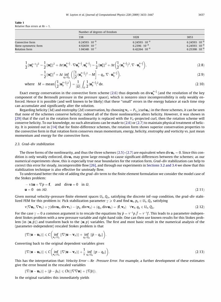
Table 1Relative flux errors at Re ¼ 1.

Number of degrees of freedom

338 1028 3853

Convective form 6:24593 � 10�8 6:24593 � 10�8 6:24593 � 10�8

Skew-symmetric form 4:92659 � 10�7 6:2396 � 10�8 6:24593 � 10�8

Rotation form 1:04348 � 10�7 6:42264 � 10�8 6:25398 � 10�8

W. Layton et al. / Journal of Computational Physics 228 (2009) 3433–3447 3437

12kunþ1

h k2 ¼ 12kun

hk2 þ Dtðunþ1

2h � runþ1

2h ;unþ1

2h Þ ¼

12kun

hk2 þ Dt

12ðunþ1

2h Þ

2;r � unþ1

2h

� �; ð2:8Þ

¼ 12kun

hk2 þ Dt inf

qh2Qh

12ðunþ1

2h Þ

2 �M� �

� qh;r � unþ1

2h

� �; ð2:9Þ

where M ¼mean12junþ1

2h j

2� �

¼ 1jXj

ZX

12junþ1

2h j

2 dx: ð2:10Þ

Exact energy conservation in the convective form scheme (2.6) thus depends on divunþ12

h (and the resolution of the keycomponent of the Bernoulli pressure in the pressure space), which is nonzero since incompressibility is only weakly en-forced. Hence it is possible (and well known to be likely) that these ‘‘small” errors in the energy balance at each time stepcan accumulate and significantly alter the solution.

Regarding helicity (3d) and enstrophy (2d) conservation, by choosing vh ¼ PVhðcurluhÞ in the three schemes, it can be seen

that none of the schemes conserve helicity; indeed all of the three nonlinearities alters helicity. However, it was shown in[29] that if the curl in the rotation form nonlinearity is replaced with the Vh-projected curl, then the rotation scheme willconserve helicity. To our knowledge, no such alterations can be made to (2.6) or (2.7) to maintain physical treatment of helic-ity. It is pointed out in [14] that for finite-difference schemes, the rotation form shows superior conservation properties tothe convective form in that rotation form conserves mean momentum, energy, helicity, enstrophy and vorticity vs. just meanmomentum and energy for the convective form.

2.3. Grad–div stabilization

The three forms of the nonlinearity, and thus the three schemes (2.5)–(2.7) are equivalent when divuh ¼ 0. Since this con-dition is only weakly enforced, divuh may grow large enough to cause significant differences between the schemes; as ournumerical experiments show, this is especially true near boundaries for the rotation form. Grad–div stabilization can help tocorrect this error for steady, incompressible flow [26], and through our experiments in Sections 3.2 and 3.4 we show that thisstabilization technique is also effective for unsteady flow.

To understand better the role of adding the grad–div term to the finite element formulation we consider the model case ofthe Stokes problem:

� mDuþrp ¼ f; and divu ¼ 0 in X;

u ¼ 0 on @X: ð2:11Þ

Given normal velocity–pressure finite element spaces Uh;Q h, satisfying the discrete inf–sup condition, the grad–div stabi-lized FEM for this problem is: Pick stabilization parameter c P 0 and find uh; ph 2 Uh;Q h satisfying

mðruh;rvhÞ þ cðdivuh;divvhÞ � ðph;divvhÞ þ ðqh;divuhÞ ¼ ðf;vhÞ 8vh; qh 2 Uh;Q h: ð2:12Þ

For the case c ¼ 0 a common argument is to rescale the equations by ~p ¼ m�1p;~f ¼ m�1f . This leads to a parameter-indepen-dent Stokes problem with a new pressure variable and right-hand side. One can then use known results for this Stokes prob-lem (in u; ~pf g) and transform back to the fu; pg variables. The first and most basic result in the numerical analysis of the(parameter-independent) rescaled Stokes problem is that

krðu� uhÞk 6 C infvh2Uh

krðu� vhÞk þ infqh2Qh

k~p� qhk� �

:

Converting back to the original dependent variables gives

krðu� uhÞk 6 C infvh2Uh

krðu� vhÞk þ1m

infqh2Qh

kp� qhk� �

: ð2:13Þ

This has the interpretation that: Velocity Error � Re � Pressure Error. For example, a further development of these estimatesgive the error bound in the rescaled variables

krðu� uhÞk þ k~p� ~phk 6 Ch krruk þ kr~pkð Þ:

In the original variables this immediately yields

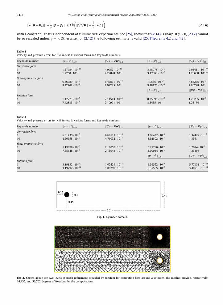
Table 2Velocity

Reynold

Convect110

Skew-sy110

Rotation110

Table 3Velocity

Reynold

Convect110

Skew-sy110

Rotation110

Fig. 2.14,455,

3438 W. Layton et al. / Journal of Computational Physics 228 (2009) 3433–3447

krðu� uhÞk þ1mkp� phk 6 Ch krruk þ 1

mkrpk

� �ð2:14Þ

with a constant C that is independent of m. Numerical experiments, see [25], shows that (2.14) is sharp. If c > 0, (2.12) cannotbe so rescaled unless c ¼ m. Otherwise, for (2.12) the following estimate is valid [25, Theorems 4.2 and 4.3]:

and pressure errors for NSE in test 1: various forms and Reynolds numbers.

s number ku� uhk1;0 kru�ruhk2;0 kp� phk1;0 krp�rphk2;0

ive form1:27984 � 10�11 4:0987 � 10�11 3:48078 � 10�9 2:02411 � 10�10

1:2750 � 10�11 4:22028 � 10�11 3:17668 � 10�9 1:26608 � 10�10

mmetric form6:56789 � 10�5 6:42861 � 10�4 1:0656 � 10�2 4:84275 � 10�3

8:42768 � 10�2 7:99285 � 10�1 9:18175 � 10�1 7:86798 � 10�1

kP � Phk1;0 kjrP �rPhjk2;0

form1:17773 � 10�5 2:14543 � 10�4 8:35095 � 10�3 1:26205 � 10�2

7:42883 � 10�3 2:10991 � 10�1 8:3435 � 10�1 1.26174

and pressure errors for NSE in test 2: various forms and Reynolds numbers.

s number ku� uhk1;0 kru�ruhk2;0 kp� phk1;0 krp�rphk2;0

ive form6:51439 � 10�5 6:66111 � 10�4 1:06432 � 10�2 1:34122 � 10�2

4:50658 � 10�2 4:76032 � 10�1 8:92802 � 10�1 1.3361

mmetric form1:19698 � 10�5 2:18059 � 10�4 3:71786 � 10�4 1:2624 � 10�2

7:65648 � 10�3 2:15944 � 10�1 3:90984 � 10�2 1.26198

kP � Phk1;0 krP �rPhk2;0

form3:19832 � 10�12 1:05429 � 10�11 9:36552 � 10�6 5:77438 � 10�11

3:19792 � 10�12 1:08799 � 10�11 9:35505 � 10�5 3:40516 � 10�11

Fig. 1. Cylinder domain.

Shown above are two levels of mesh refinement provided by Freefem for computing flow around a cylinder. The meshes provide, respectively,and 56,702 degrees of freedom for the computations.

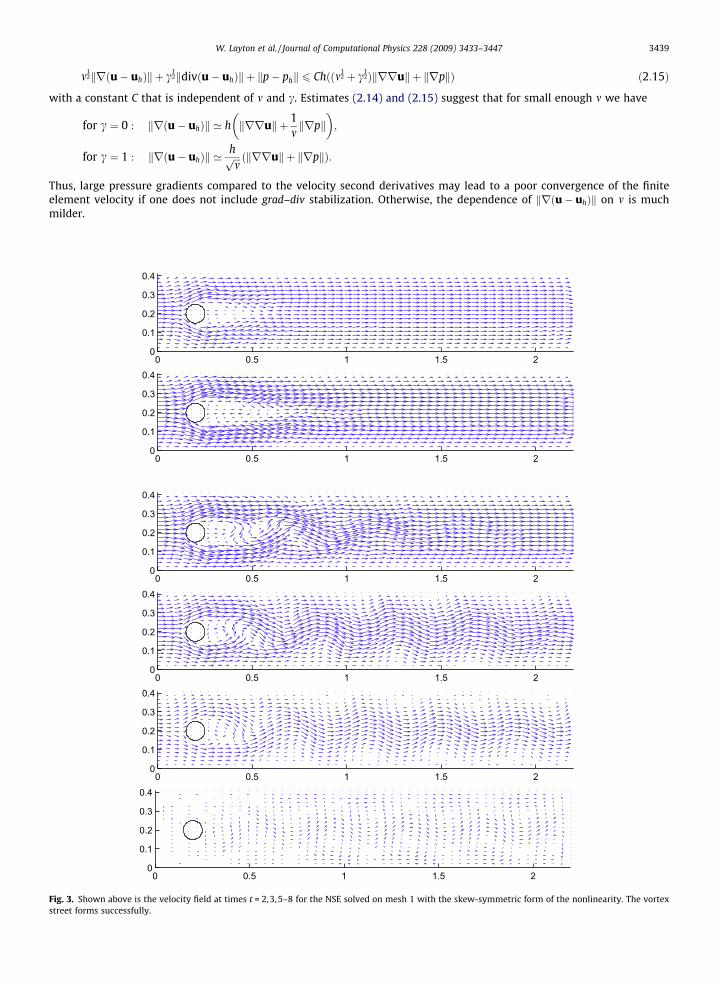
Fig. 3.street f

W. Layton et al. / Journal of Computational Physics 228 (2009) 3433–3447 3439

m12krðu� uhÞk þ c1

2kdivðu� uhÞk þ kp� phk 6 Chððm12 þ c1

2Þkrruk þ krpkÞ ð2:15Þ

with a constant C that is independent of m and c. Estimates (2.14) and (2.15) suggest that for small enough m we have

for c ¼ 0 : krðu� uhÞk ’ h krruk þ 1mkrpk

� �;

for c ¼ 1 : krðu� uhÞk ’hffiffiffimp krruk þ krpkð Þ:

Thus, large pressure gradients compared to the velocity second derivatives may lead to a poor convergence of the finiteelement velocity if one does not include grad–div stabilization. Otherwise, the dependence of krðu� uhÞk on m is muchmilder.

0 0.5 1 1.5 20

0.1

0.2

0.3

0.4

0 0.5 1 1.5 20

0.1

0.2

0.3

0.4

0 0.5 1 1.5 20

0.1

0.2

0.3

0.4

0 0.5 1 1.5 20

0.1

0.2

0.3

0.4

0 0.5 1 1.5 20

0.1

0.2

0.3

0.4

0 0.5 1 1.5 20

0.1

0.2

0.3

0.4

Shown above is the velocity field at times t = 2,3,5–8 for the NSE solved on mesh 1 with the skew-symmetric form of the nonlinearity. The vortexorms successfully.

3440 W. Layton et al. / Journal of Computational Physics 228 (2009) 3433–3447

3. Three numerical experiments

We consider three carefully chosen examples that, we believe, give strong support for the scenario of accuracy loss de-scribed in the introduction. We use the software FreeFem++ [13] to run the numerical tests. The models are discretized withthe Crank–Nicolson method in time and with the Taylor–Hood finite elements (continuous piecewise quadratic polynomialsfor the velocity and linears for the pressure) in space; the nonlinear system is solved by a fixed point iteration.

3.1. Test 1: Poiseuille flow

In X ¼ ð0;4Þ � ð0;1Þ, a parabolic inflow v(x,y, t) = 0 and uðx; y; tÞ ¼ 12m yð1� yÞ (at x = 0) is prescribed. No-slip boundary con-

ditions are given at the top and bottom, and the do-nothing boundary condition is prescribed at the outflow. The exact solu-tion is well known to be vðx; yÞ ¼ 0;uðx; yÞ ¼ 1

2m yð1� yÞ; pðx; yÞ ¼ �xþ 4, and we take it as our initial condition. A discussion

0 0.5 1 1.5 20

0.1

0.2

0.3

0.4

0 0.5 1 1.5 20

0.1

0.2

0.3

0.4

0 0.5 1 1.5 20

0.1

0.2

0.3

0.4

0 0.5 1 1.5 20

0.1

0.2

0.3

0.4

0 0.5 1 1.5 20

0.1

0.2

0.3

0.4

0 0.5 1 1.5 20

0.1

0.2

0.3

0.4

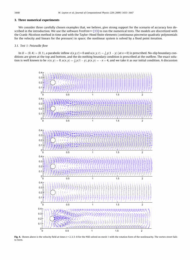
Fig. 4. Shown above is the velocity field at times t = 2,3,5–8 for the NSE solved on mesh 1 with the rotation form of the nonlinearity. The vortex street failsto form.

W. Layton et al. / Journal of Computational Physics 228 (2009) 3433–3447 3441

of this problem can be found in Canuto et al. [6]. The key conserved quantity in the flow is the flux through any cross sectiongiven by

Fig

QðxÞ ¼Z

0<y<1uðx; yÞdy ¼ 1

12m:

Note that u ¼ ðu;vÞ and p are in the finite element spaces so that we expect that discretization of the convective andskew-symmetric form of the NSE will have very small errors (comparable to the errors from numerical integration and solu-tion of the linear and nonlinear systems arising). On the other hand, if the rotation form is used the exact solution is

vðx; yÞ ¼ 0;

uðx; yÞ ¼ 12m

yð1� yÞ;

Pðx; yÞ ¼ pðx; yÞ þ 18m2 y2ð1� yÞ2

0 0.5 1 1.5 20

0.1

0.2

0.3

0.4

0 0.5 1 1.5 20

0.1

0.2

0.3

0.4

0 0.5 1 1.5 20

0.1

0.2

0.3

0.4

0 0.5 1 1.5 20

0.1

0.2

0.3

0.4

0 0.5 1 1.5 20

0.1

0.2

0.3

0.4

0 0.5 1 1.5 20

0.1

0.2

0.3

0.4

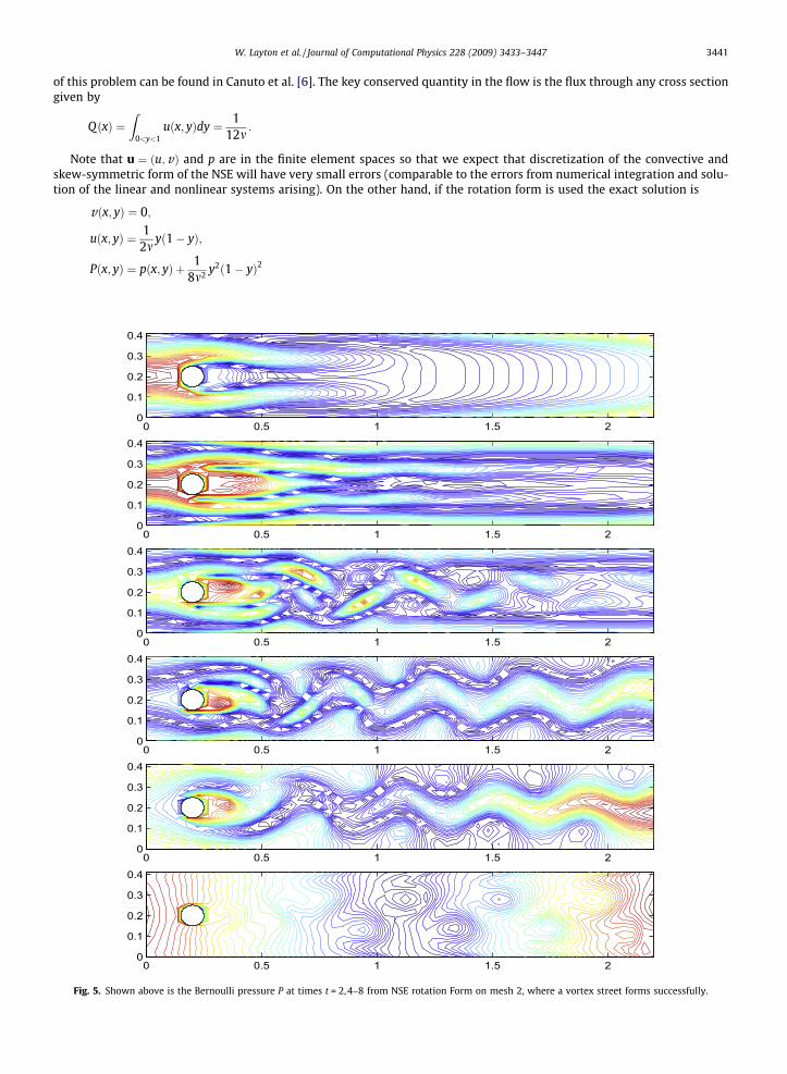
. 5. Shown above is the Bernoulli pressure P at times t = 2,4–8 from NSE rotation Form on mesh 2, where a vortex street forms successfully.

3442 W. Layton et al. / Journal of Computational Physics 228 (2009) 3433–3447

is not in the pressure finite element space. Thus, in the rotation form there will be discretization errors in p that influence aswell the velocity error through the discrete momentum equation, since

Fig. 6

P R Q h and kPk ¼ Oðm�2Þ: ð3:1Þ

To test Poiseuille flow we take the time step Mt ¼ 0:01 and number of time steps = 100, so the final time is T ¼ 1.For the flux computations we find that expressing the nonlinearity in different forms does not affect the true value of the

flux for Re = 1. Results are presented in Table 1.Next we test the coupling between velocity and pressure errors by computing the error on a fixed mesh for Re ¼ 1 and

Re ¼ 10 (decreasing m). We present the results at the final time T ¼ 1 and at the mesh level with number of degrees of free-dom being 1028 in Table 2.

From Table 2, the convective form of NSE performs best with respect to the size of the velocity and pressure errors. Thevelocity and pressure errors for the skew-symmetric form are bigger than the corresponding errors for the convective form.It is known that skew-symmetric form of the nonlinear term of NSE imposes difficulties for simulation of Poiseuille flow[11,16], which we also observe here.

0 0.5 1 1.5 20

0.1

0.2

0.3

0.4

0 0.5 1 1.5 20

0.1

0.2

0.3

0.4

0 0.5 1 1.5 20

0.1

0.2

0.3

0.4

0 0.5 1 1.5 20

0.1

0.2

0.3

0.4

0 0.5 1 1.5 20

0.1

0.2

0.3

0.4

0 0.5 1 1.5 20

0.1

0.2

0.3

0.4

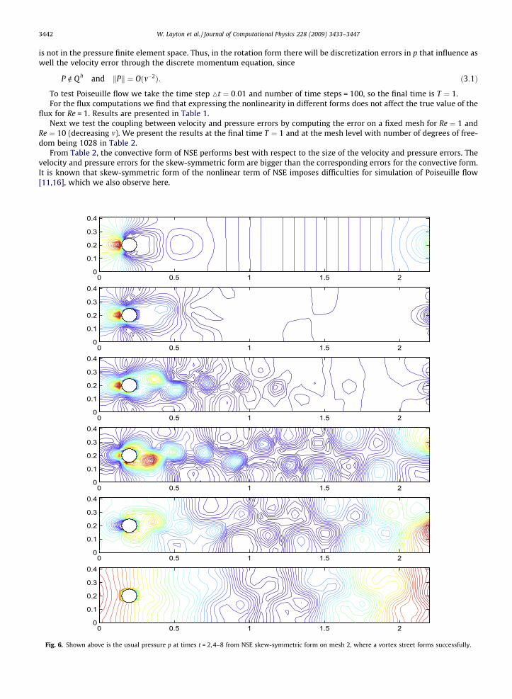
. Shown above is the usual pressure p at times t = 2,4–8 from NSE skew-symmetric form on mesh 2, where a vortex street forms successfully.

W. Layton et al. / Journal of Computational Physics 228 (2009) 3433–3447 3443

We also observe that while the velocity errors are smaller for the rotation form compared to the skew-symmetricform, the error in the (Bernoulli) pressure gradient is larger than the (usual) pressure gradient error of the skew-sym-metric form. Note that for rotation form, the pressure error kp� phk1;0 and the velocity error krðu� uhÞk2;0 seem toscale like Re3, and ku� uhk1;0 seems to scale like Re2. Poor scaling with Re can be improved in the case of Stokesand rotation form steady NSE with the use of grad–div stabilization, and is our motivation in later test problems touse this stabilization.

3.2. Test 2: Resolution vs. nonlinearity

The relative importance of resolution of pressures vs. nonlinearity can be tested by artificially reversing p and P in Test 1in a (completely) synthetic test problem. Thus, we take:

Fig. 7.Bernouthe dev

uðx; yÞ ¼ 12m

yð1� yÞ; vðx; yÞ ¼ 0; Pðx; yÞ ¼ �xþ 4;

so that

pðx; yÞ ¼ �xþ 4� 18m2 y2ð1� yÞ2:

These are inserted in the Navier–Stokes equations to obtain a right-hand side f ¼ fðx; y; mÞ:

fðx; y; mÞ :¼ 0;1

4m2 y2ð1� yÞ � yð1� yÞ2 � �T

:

The resolution of p vs. P is exactly reversed from Test 1. We present the error behavior at the final time T ¼ 1 and at the meshlevel with number of degrees of freedom being 1028 in Table 3.

Table 3 shows that discretization errors are present if the solution does not belong to the finite element space. Thecomputed errors from Test 2 are the mirror image (up to the preset accuracy used for the various linear and nonlineariterative solvers’ stopping criteria) of the error behavior in the previous test. Thus it is clear that, without grad–div sta-bilization, in the rotation form it is the resolution of the Bernoulli pressure determine the quality of the overall velocityapproximation.

3.3. Test 3: Flow around a cylinder

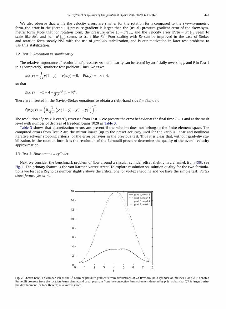
Next we consider the benchmark problem of flow around a circular cylinder offset slightly in a channel, from [30], seeFig. 1. The primary feature is the von Karman vortex street. To explore resolution vs. solution quality for the two formula-tions we test at a Reynolds number slightly above the critical one for vortex shedding and we have the simple test: Vortexstreet formed yes or no.

0 1 2 3 4 5 6 7 80

2

4

6

8

10

12

14

16

t

grad p, mesh 2grad p, mesh 1grad P, mesh 2grad P, mesh 1

Shown here is a comparison of the L2 norm of pressure gradients from simulations of 2d flow around a cylinder on meshes 1 and 2. P denotedlli pressure from the rotation form scheme, and usual pressure from the convective form scheme is denoted by p. It is clear that rP is larger duringelopment (or lack thereof) of a vortex street.

3444 W. Layton et al. / Journal of Computational Physics 228 (2009) 3433–3447

The time dependent inflow and outflow profile are

Fig. 8.stabiliz

u1ð0; y; tÞ ¼ u1ð2:2; y; tÞ ¼6

0:412 sinðpt=8Þyð0:41� yÞ;

u2ð0; y; tÞ ¼ u2ð2:2; y; tÞ ¼ 0:

No-slip boundary conditions are prescribed along the top and bottom walls and the initial condition is uðx; y;0Þ ¼ 0. The vis-cosity is set at m ¼ 10�3, the external force f ¼ 0, and the Reynolds number of the flow, based on the diameter of the cylinderand on the mean velocity inflow is 0 6 Re 6 100. The time step is chosen to be Dt ¼ 0:005.

Freefem generated two Delaunay meshes for testing this problem, the finest of which is able to resolve the problem forthe NSE in either (rotation or skew-symmetric) form. These are shown in Fig. 2.

The velocity field calculated on mesh 1 is shown in Figs. 3 and 4. Note that

� with the skew-symmetric form the vortex street is well defined already on mesh 1 (coarse mesh);� with the rotation form the mesh 1 simulations fails;� with the rotation form and grad–div stabilization, the mesh 1 simulation forms a vortex street.

0 0.5 1 1.5 20

0.1

0.2

0.3

0.4

0 0.5 1 1.5 20

0.1

0.2

0.3

0.4

0 0.5 1 1.5 20

0.1

0.2

0.3

0.4

0 0.5 1 1.5 20

0.1

0.2

0.3

0.4

0 0.5 1 1.5 20

0.1

0.2

0.3

0.4

0 0.5 1 1.5 20

0.1

0.2

0.3

0.4

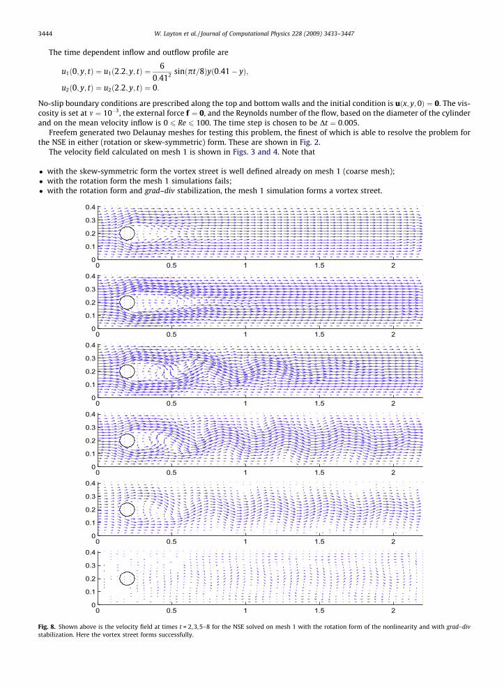
Shown above is the velocity field at times t = 2,3,5–8 for the NSE solved on mesh 1 with the rotation form of the nonlinearity and with grad–divation. Here the vortex street forms successfully.

W. Layton et al. / Journal of Computational Physics 228 (2009) 3433–3447 3445

The pressure (and accuracy thereof) is critical for the formation of the vortex street. To test the resolution hypothesis, wemove to mesh 2, which fully resolves both formulations. Figs. 5 and 6 plot p (from skew-symmetric formulation) and P (fromrotation formulation), respectively, and from these plots we see indication that P contains much smaller transition regionsthan p. The difference can also be seen when the L2 norm of rp;rP are plotted vs. time, in Fig. 7.

Fig. 8 shows the effect of the grad–div stabilization of the solution computed in mesh 1 with c ¼ 1 and the rotation form.Without the stabilization, the rotation form is unable to predict the correct behavior. With grad–div stabilization, the correctbehavior is predicted already on mesh 1.

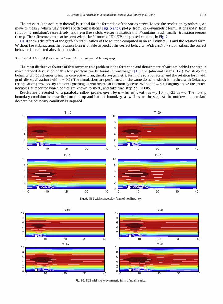
3.4. Test 4: Channel flow over a forward and backward facing step

The most distinctive feature of this common test problem is the formation and detachment of vortices behind the step (amore detailed discussion of this test problem can be found in Gunzburger [10] and John and Liakos [17]). We study thebehavior of NSE schemes using the convective form, the skew-symmetric form, the rotation form, and the rotation form withgrad–div stabilization (with c ¼ 0:5). The simulations are performed on the same domain, which is meshed with Delaunaytriangulation (provided by Freefem), yielding 24,598 degree of freedom systems. We set Re ¼ 600 (slightly above the criticalReynolds number for which eddies are known to shed), and take time step Dt ¼ 0:005.

Results are presented for a parabolic inflow profile, given by u ¼ ðu1;u2ÞT , with u1 ¼ yð10� yÞ=25;u2 ¼ 0. The no-slipboundary condition is prescribed on the top and bottom boundary, as well as on the step. At the outflow the standarddo-nothing boundary condition is imposed.

T=10

0 10 20 30 400

2

4

6

8

10 T=20

0 10 20 30 400

2

4

6

8

10

T=30

0 10 20 30 400

2

4

6

8

10T=40

0 10 20 30 400

2

4

6

8

10

Fig. 9. NSE with convective form of nonlinearity.

T=10

0 10 20 30 4002468

10 T=20

0 10 20 30 4002468

10

T=30

0 10 20 30 4002468

10T=40

0 10 20 30 4002468

10

Fig. 10. NSE with skew-symmetric form of nonlinearity.

T=10

0 10 20 30 4002468

10 T=20

0 10 20 30 4002468

10

T=30

0 10 20 30 4002468

10T=40

0 10 20 30 4002468

10

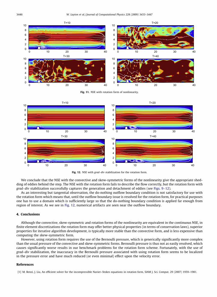
Fig. 11. NSE with rotation form of nonlinearity.

T=10

0 10 20 30 4002468

10 T=20

0 10 20 30 4002468

10

T=30

0 10 20 30 4002468

10T=40

0 10 20 30 4002468

10

Fig. 12. NSE with grad–div stabilization for the rotation form.

3446 W. Layton et al. / Journal of Computational Physics 228 (2009) 3433–3447

We conclude that the NSE with the convective and skew-symmetric forms of the nonlinearity give the appropriate shed-ding of eddies behind the step. The NSE with the rotation form fails to describe the flow correctly, but the rotation form withgrad–div stabilization successfully captures the generation and detachment of eddies (see Figs. 9–12).

As an interesting but tangential observation, the do-nothing outflow boundary condition is not satisfactory for use withthe rotation form which means that, until the outflow boundary issue is resolved for the rotation form, for practical purposesone has to use a domain which is sufficiently large so that the do-nothing boundary condition is applied far enough fromregion of interest. As we see in Fig. 12, numerical artifacts are seen near the outflow boundary.

4. Conclusions

Although the convective, skew-symmetric and rotation forms of the nonlinearity are equivalent in the continuous NSE, infinite element discretizations the rotation form may offer better physical properties (in terms of conservation laws), superiorproperties for iterative algorithm development, is typically more stable than the convective form, and is less expensive thancomputing the skew-symmetric form.

However, using rotation form requires the use of the Bernoulli pressure, which is generically significantly more complexthan the usual pressure of the convective and skew-symmetric forms. Bernoulli pressure is thus not as easily resolved, whichcauses significantly worse results in our benchmark problems for the rotation form scheme. Fortunately, with the use ofgrad–div stabilization, the inaccuracy in the Bernoulli pressure associated with using rotation form seems to be localizedin the pressure error and have much reduced (or even minimal) effect upon the velocity error.

References

[1] M. Benzi, J. Liu, An efficient solver for the incompressible Navier–Stokes equations in rotation form, SIAM J. Sci. Comput. 29 (2007) 1959–1981.

W. Layton et al. / Journal of Computational Physics 228 (2009) 3433–3447 3447

[2] E. Burman, A. Linke, Stabilized finite element schemes for incompressible flow using Scott–Vogelius elements, Appl. Numer. Math. (2007), doi:10.1016/j.apnum.2007.11.001.

[3] M. Braack, E. Burman, V. John, G. Lube, Stabilized finite element methods for the generalized Oseen problem, Comput. Methods Appl. Mech. Eng. 196(2007) 853–866.

[4] G.A. Blaisdell, E.T. Spryopolous, J.H. Qin, The effect of the formulation of the nonlinear terms on aliasing errors in spectral methods, Appl. Numer. Math.21 (3) (1996) 207–219.

[5] C. Canuto, M.Y. Hussaini, A. Quarteroni, T.A. Zang, Spectral Methods in Fluid Dynamics, Springer, Berlin, 1988.[6] C. Canuto, M.Y. Hussaini, A. Quarteroni, T.A. Zang, Spectral Methods Evolution to Complex Geometries and Applications to Fluid Dynamics, Springer,

Berlin, 2007.[7] H.C. Elman, D.J. Silvester, A.J. Wathen, Finite Elements and Fast Iterative Solvers: With Applications in Incompressible Fluid Dynamics, Numerical

Mathematics and Scientific Computation, Oxford University Press, Oxford, UK, 2005.[8] L.P. Franca, S.L. Frey, Stabilized finite element methods: II. The incompressible Navier–Stokes equations, Comput. Methods Appl. Mech. Eng. 99 (1992)

209–233.[9] P. Gresho, R. Sani, Incompressible Flow and the Finite Element Method, vol. 2, Wiley, 2000.

[10] M.D. Gunzburger, Finite Element Methods for Viscous Incompressible Flows – A Guide to Theory, Practices, and Algorithms, Academic Press, 1989.[11] J.G. Heywood, R. Rannacher, S. Turek, Artificial boundaries and flux and pressure conditions for the incompressible Navier–Stokes equations, Int. J.

Numer. Methods Fluids 22 (1996) 325–352.[12] P. Hansbo, A. Szepessy, A velocity–pressure streamline diffusion method for the incompressible Navier–Stokes equations, Comput. Methods Appl.

Mech. Eng. 84 (1990) 175–192.[13] F. Hecht, O. Pironneau, FreeFem++ webpage. <http://www.freefem.org>.[14] K. Horiuti, Comparison of conservative and rotation forms in large eddy simulation of turbulent channel flow, J. Comput. Phys. 71 (1987) 343–370.[15] K. Horiuti, T. Itami, Truncation error analysis of the rotation form of convective terms in the Navier–Stokes equations, J. Comput. Phys. 145 (1998) 671–

692.[16] V. John, Large eddy simulation of turbulent incompressible, analytical and numerical results for a class of LES models, Lecture Notes in Computational

Science and Engineering, vol. 34, Springer-Verlag, Berlin, Heidelberg, New York, 2004.[17] V. John, A. Liakos, Time dependent flow across a step: the slip with friction boundary condition, Int. J. Numer. Methods Fluids 50 (2006) 713–731.[18] C.A. Kennedy, A. Gruber, Reduced aliasing formulations of the convective terms within the Navier–Stokes equations for a compressible fluid, J. Comput.

Phys. 227 (2008) 16761700.[19] A.G. Kravchenko, P. Moin, On the effect of numerical errors in large eddy simulations of turbulent flows, J. Comput. Phys. 131 (2) (1997) 310–322.[20] W. Layton, C. Manica, M. Neda, L. Rebholz, Numerical analysis and computational comparisons of the NS-alpha and NS-omega regularizations, Comput.

Methods Appl. Mech. Eng., in press, doi:10.1016/j.cma.2009.01.011.[21] G. Lube, M. Olshanskii, Stable finite element calculations of incompressible flows using the rotation form of convection, IMA J. Numer. Anal. 22 (2002)

437–461.[22] G. Matthies, G. Lube, On streamline-diffusion methods of inf–sup stable discretizations of the generalized Oseen problem, Preprint 2007-02, Institute

Numerische und Angewandte Mathematik, Georg-August-Universiat Gottingen, 2007.[23] G. Matthies, L. Tobiska, Local projection type stabilization applied to inf–sup stable discretizations of the Oseen problem, Preprint 47/2007, Dept.

Math., Otto-von-Guericke-Universitat Magdeburg, 2007.[24] R.D. Moser, P. Moin, The effects of curvature in wall bounded flows, J. Fluid Mech. 175 (1987) 479–510.[25] M.A. Olshanskii, A. Reusken, Grad–div stabilization for the Stokes equations, Math. Comput. 73 (2004) 1699–1718.[26] M.A. Olshanskii, A low order Galerkin finite element method for the Navier–Stokes equations of steady incompressible flow: a stabilization issue and

iterative methods, Comput. Methods Appl. Mech. Eng. 191 (2002) 5515–5536.[27] M.A. Olshanskii, A. Reusken, Navier–Stokes equations in rotation form: a robust multigrid solver for the velocity problem, SIAM J. Sci. Comput. 23

(2002) 1682–1706.[28] M.A. Olshanskii, Iterative solver for Oseen problem and numerical solution of incompressible Navier–Stokes equations, Numer. Linear Algebra Appl. 6

(1999) 353–378.[29] L. Rebholz, An energy and helicity conserving finite element scheme for the Navier–Stokes equations, SIAM J. Numer. Anal. 45 (4) (2007) 1622–1638.[30] M. Shäfer, S. Turek, Benchmark computations of laminar flow around cylinder, Flow Simulation with High-Performance Computers, vol. II, Vieweg,

1996.[31] L. Tobiska, G. Lube, A modified streamline diffusion method for solving the stationary Navier–Stokes equations, Numer. Math. 59 (1991) 13–29.[32] D. Wilhelm, L. Kleiser, Stable and unstable formulations of the convection operator in spectral element simulations, Appl. Numer. Math. 33 (14) (2000)

275–280.[33] T.A. Zang, On the rotation and skew-symmetric forms for incompressible flow simulations, Appl. Numer. Math. 7 (1991) 27–40.