Embed Size (px)
Citation preview
Volume 2 No.7, JULY 2011 ISSN 2079-8407
Journal of Emerging Trends in Computing and Information Sciences
©2010-11 CIS Journal. All rights reserved.
http://www.cisjournal.org
332
Algorithms in "UniModBase" Information System for determine Rosin-
Rammler and Gaudin-Shumann equations of particle size distribution
using regression analysis
1SAŠA PUŠICA,
2VELIMIR ŠĆEKIĆ,
3MILUNKA PUŠICA
1M.Sc.., Agencija "Smaj Business", Crnovrških brigada 6/1, 19210 Bor, Serbia 2prof. D.Sc., FIM, Majke Jugovića 4, 37000 Kruševac, Serbia
3B.Sc., Regionalni centar za talente Bor, 3.oktobar 71, 19210 Bor, Serbia
ABSTRACT
"UniModBase" is freeware information systems for modeling of grain size analysis and determine Rosin-Rammler and
Gaudin-Shumann equations of particle size distribution based on algorithms for regression analysis. The algorithm is
precisely defined procedures and instructions how to solve a task or problem, and this paper show the algorithms for
determine the Rosin-Rammler and Gaudin-Schuhmann equation using regresion analysis. Author of this paper these
algorithms used as starting point in the construction of "UniModBase" information system.
Keywords— Information system, algorithm, regression analysis, Rosin-Rammler, Gaudin-Schuhmann
1. INTRODUCTION
Grain size of sample is a mixture of grains with
different shape and size in narrow size class. Narrow size
class contains the grains whose particle diameter is in the
range of class between d1 to d2. This range depends on the
methods and devices for determine the particle size
distribution [1].
Sieve analysis is one of method for determine the
composition of the raw material, where this material is
classified according to geometric size of grains. Sieving
through the sieve, the sample is classified into two class
size. Large classes with pieces of grain that is greater than
the holes of sieve, is retained on the sieve. Small class
with grains smaller than the holes of sieve, passing
through the sieve. Sieving of sample on multiple sieve
from a series (Fig.1) obtained narrow size class of sample.
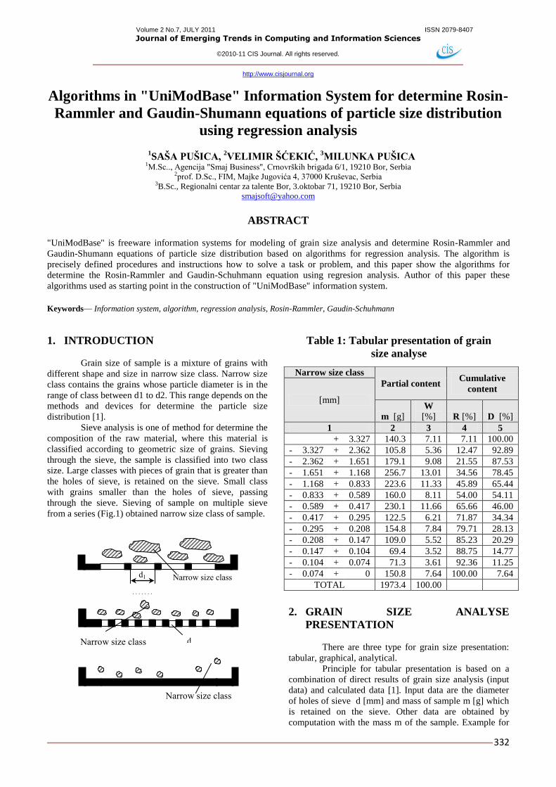
Table 1: Tabular presentation of grain
size analyse
2. GRAIN SIZE ANALYSE
PRESENTATION
There are three type for grain size presentation:
tabular, graphical, analytical.
Principle for tabular presentation is based on a
combination of direct results of grain size analysis (input
data) and calculated data [1]. Input data are the diameter
of holes of sieve d [mm] and mass of sample m [g] which
is retained on the sieve. Other data are obtained by
computation with the mass m of the sample. Example for
Narrow size class
Partial content Cumulative
content
[mm]
m [g] W
[%] R [%] D [%]
1 2 3 4 5
+ 3.327 140.3 7.11 7.11 100.00
- 3.327 + 2.362 105.8 5.36 12.47 92.89
- 2.362 + 1.651 179.1 9.08 21.55 87.53
- 1.651 + 1.168 256.7 13.01 34.56 78.45
- 1.168 + 0.833 223.6 11.33 45.89 65.44
- 0.833 + 0.589 160.0 8.11 54.00 54.11
- 0.589 + 0.417 230.1 11.66 65.66 46.00
- 0.417 + 0.295 122.5 6.21 71.87 34.34
- 0.295 + 0.208 154.8 7.84 79.71 28.13
- 0.208 + 0.147 109.0 5.52 85.23 20.29
- 0.147 + 0.104 69.4 3.52 88.75 14.77
- 0.104 + 0.074 71.3 3.61 92.36 11.25
- 0.074 + 0 150.8 7.64 100.00 7.64
TOTAL 1973.4 100.00 Narrow size class
- dmax + d1 . . . . . . .
d
n
Narrow size class
- dn-1 + dn
Narrow size class
- dn + 0
d1
Volume 2 No.7, JULY 2011 ISSN 2079-8407
Journal of Emerging Trends in Computing and Information Sciences
©2010-11 CIS Journal. All rights reserved.
http://www.cisjournal.org
333
tabular presentation is showed in Table 1. Calculated data
in this table refer to the mass of size class and they are: W
- mass of size class [%], R - cumulative content of mass
retained on sieve [%], D - cumulative content of mass that
passed through the sieve [%]
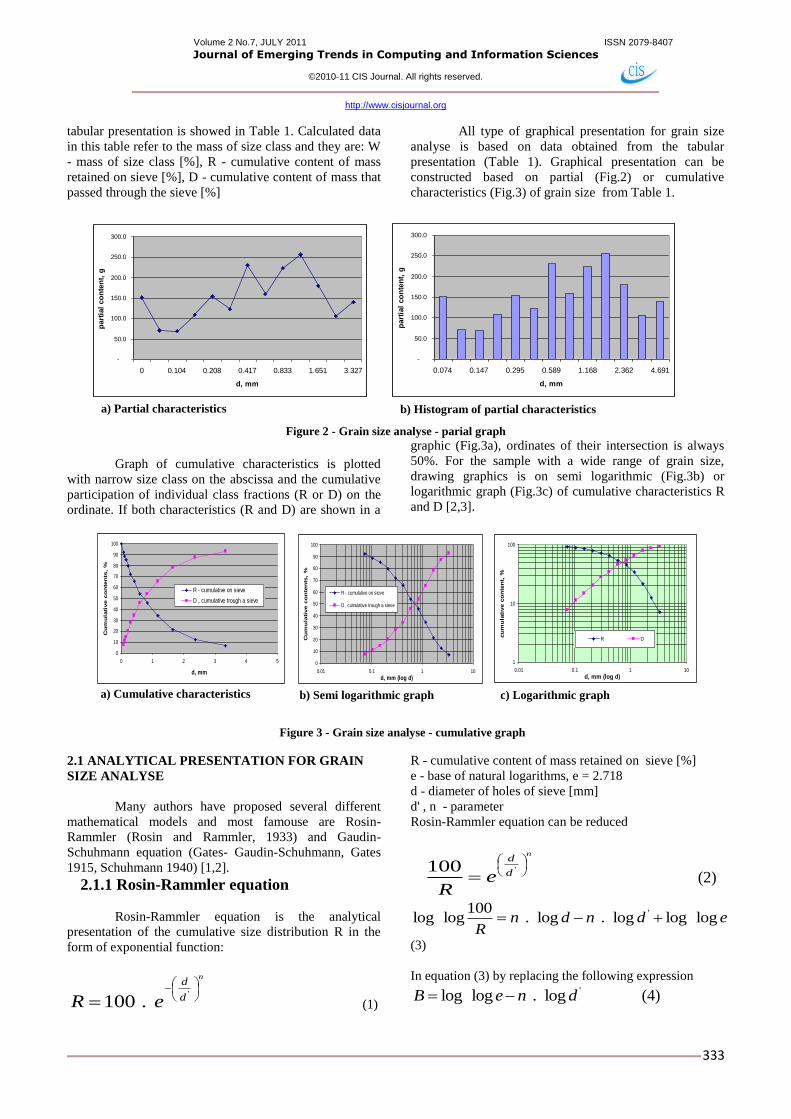
All type of graphical presentation for grain size
analyse is based on data obtained from the tabular
presentation (Table 1). Graphical presentation can be
constructed based on partial (Fig.2) or cumulative
characteristics (Fig.3) of grain size from Table 1.
Figure 2 - Grain size analyse - parial graph
Graph of cumulative characteristics is plotted
with narrow size class on the abscissa and the cumulative
participation of individual class fractions (R or D) on the
ordinate. If both characteristics (R and D) are shown in a
graphic (Fig.3a), ordinates of their intersection is always
50%. For the sample with a wide range of grain size,
drawing graphics is on semi logarithmic (Fig.3b) or
logarithmic graph (Fig.3c) of cumulative characteristics R
and D [2,3].
Figure 3 - Grain size analyse - cumulative graph
2.1 ANALYTICAL PRESENTATION FOR GRAIN
SIZE ANALYSE
Many authors have proposed several different
mathematical models and most famouse are Rosin-
Rammler (Rosin and Rammler, 1933) and Gaudin-
Schuhmann equation (Gates- Gaudin-Schuhmann, Gates
1915, Schuhmann 1940) [1,2].
2.1.1 Rosin-Rammler equation
Rosin-Rammler equation is the analytical
presentation of the cumulative size distribution R in the
form of exponential function:
n
d
d
eR
'
.100 (1)
R - cumulative content of mass retained on sieve [%]
e - base of natural logarithms, e = 2.718
d - diameter of holes of sieve [mm]
d' , n - parameter
Rosin-Rammler equation can be reduced
n
d
d
eR
'100
(2)
edndnR
logloglog.log.100
loglog '
(3)
In equation (3) by replacing the following expression 'log.loglog dneB (4)
-
50.0
100.0
150.0
200.0
250.0
300.0
0 0.104 0.208 0.417 0.833 1.651 3.327
d, mm
part
ial
co
nte
nt,
g
-
50.0
100.0
150.0
200.0
250.0
300.0
0.074 0.147 0.295 0.589 1.168 2.362 4.691
d, mm
part
ial
co
nte
nt,
g
a) Partial characteristics b) Histogram of partial characteristics
0
10
20
30
40
50
60
70
80
90
100
0 1 2 3 4 5
d, mm
Cu
mu
lati
ve c
on
ten
ts,
%
R - cumulative on sieve
D , cumulative trough a sieve
0
10
20
30
40
50
60
70
80
90
100
0.01 0.1 1 10
d, mm (log d)
Cu
mu
lati
ve c
on
ten
ts,
%
R - cumulative on sieve
D , cumulative trough a sieve
1
10
100
0.01 0.1 1 10
d, mm (log d)
cu
mu
lati
ve c
on
ten
t, %
R D
a) Cumulative characteristics b) Semi logarithmic graph c) Logarithmic graph
Volume 2 No.7, JULY 2011 ISSN 2079-8407
Journal of Emerging Trends in Computing and Information Sciences
©2010-11 CIS Journal. All rights reserved.
http://www.cisjournal.org
334
We gets the Rosin-Rammler equation of straight
line in the coordinate system of log d, log log shown in
Figure 4.
With graphical method it is possible to determine
the value of n , d' parameters (Fig.5) where the choice of
representative points for line p is subjective choice. This is
the main reason for define algorithm to determine Rosin-
Rammler equation using regression analysis - precision to
avoid subjective errors with graphical method.
Figure 4 - Example of graph in a coordinate
Figure 5 - Graphic principle for determining n, d'
parameters of Rosin-Rammler equation [Error! Reference
source not found.]
2.1.2 Gaudin-Schuhmann equation
Gaudin-Schuhmann equation is the analytical
presentation of cumulative size distribution:
m
d
dD
max
.100 (5)
D - cumulative content of mass that passed through the
sieve [%]
d - diameter of holes of sieve [mm]
dmax - diameter of holes of sieve that passed 100% of
sample [mm]
Gaudin-Schuhmann equations can be reduced
maxlog.log.2log dmdmD (6)
In equation (6) by replacing the following expression
maxlog.2 dmA (7)
We get the Gaudin-Schuhmann equation of
straight line in the coordinate system of log d, log D
shown in Figure 6. The value of m parameters (Fig.7) is
possible to determine with graphical method where the
choice of representative points and angle for line is
subjective choice. To avoid subjective errors with
graphical method, we can define algorithm to determine
Gaudin-Schuhmann equation using regression analysis.
Figure 6 - Example of graph in a coordinate system log d , log
D
3. REGRESSION ANALYSIS
3.1 Linear regression
A linear relationship y = ax + b is the simplest
mathematical model of the functional dependence of
related variables. The parameter a is called the regression
coefficient, while the parameter b represents the value of a
regression function when the independent variable equals
zero [4,6,9]. To determine this parameters, it is assumed
that the values of variable yi associated with the values of
the independent variable xi as follows:
(8)
x1, x2, .... xn - measured values of
independent variables
y1, y2, .... yn - measured values of
dependent variables
Numerical values of the dependent variable is
obtained when the equation (8) incorporate the measured
values of independent variables:
(9)
0
0.5
1
1.5
2
2.5
-1.5 -1 -0.5 0 0.5 1
log d
log
D
Volume 2 No.7, JULY 2011 ISSN 2079-8407
Journal of Emerging Trends in Computing and Information Sciences
©2010-11 CIS Journal. All rights reserved.
http://www.cisjournal.org
335
Differences between measured and theoretical
values of the dependent variable represent the deviation of
this mathematical model:
(10)
For a minor deviation, the calculated
values of the dependent variables are very close
to measured values and the proposed
mathematical model adequately demonstrates
the measured data.
According to this principle, model y = ax
+ b is the most accurate when the sum of
squared deviations is minimal:
n
i
n
i
iii bxaybaf1 1
22).(),( (11)
The sum of squared deviations is
minimal if the conditions are met:
(12)
We get the system of two equations with
two unknowns a, b parameters for mathematical
model:
(13)
(14)
(15)
(16)
These equations can be simplified by
introducing the following expressions:
(17)
(18)
The parameters a, b of mathematical model is
now calculated:
(19)
(20)
In accordance with these principles of linear
regression, is defined and on Figure 8 is presented the
algorithm for determining the coefficients a, b of linear
regression (KOEF_A, KOEF_B) to be applied in
determining the Rosin-Rammler and Gaudin-Schuhmann
equation.
n
i
ix xS1
n
i
ixx xS1
2
n
i
iy yS1
n
i
iixy yxS1
. 2. xxx SSnDE
DE
SSSna
yxxy ..
DE
SSSSb
xyxyxx ..
N
SX = 0, SY = 0, SXX = 0, SXY= 0, I = 1
I > N NO YES
END
DE = N * SXX - SX * SX
KOEF_A = ( N*SXY - SX*SY) / DE
KOEF_B = ( SXX*SY - SX*SXY ) / DE
KOEF_A, KOEF_B
SX = SX + XI
SY = SY + YI
SXX = SXX + XI * XI
SXY = SXY + XI * YI
I = I + 1
LINREG
Volume 2 No.7, JULY 2011 ISSN 2079-8407
Journal of Emerging Trends in Computing and Information Sciences
©2010-11 CIS Journal. All rights reserved.
http://www.cisjournal.org
336
Figure 8 - The algorithm for determining the coefficients of linear regression
3.2 The coefficient of determination and
correlation coefficient
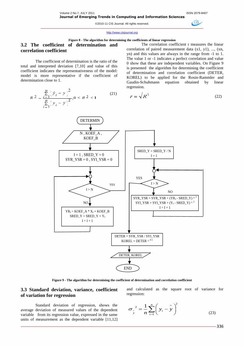
The coefficient of determination is the ratio of the
total and interpreted deviation [7,10] and value of this
coefficient indicates the representativeness of the model:
model is more representative if the coefficient of
determination close to 1.
(21)
The correlation coefficient r measures the linear
correlation of paired measurement data (x1, y1), ..., (xn,
yn) and this values are always in the range from -1 to 1.
The value 1 or -1 indicates a perfect correlation and value
0 show that these are independent variables. On Figure 9
is presented the algorithm for determining the coefficient
of determination and correlation coefficient (DETER,
KOREL) to be applied for the Rosin-Rammler and
Gaudin-Schuhmann equation obtained by linear
regression.
(22)
Figure 9 - The algorithm for determining the coefficient of determination and correlation coefficient
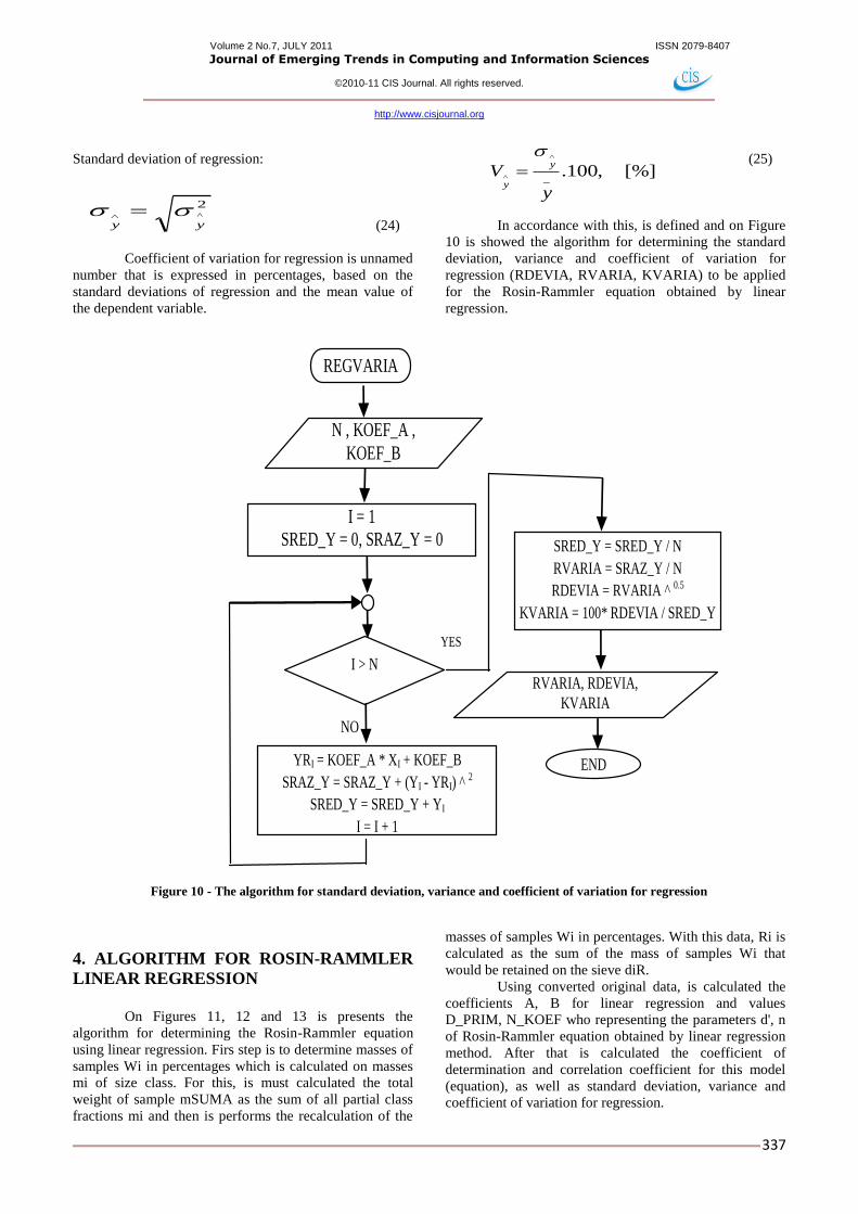
3.3 Standard deviation, variance, coefficient
of variation for regression
Standard deviation of regression, shows the
average deviation of measured values of the dependent
variable from its regression value, expressed in the same
units of measurement as the dependent variable [11,12]
and calculated as the square root of variance for
regression:
(23)
N , KOEF_A ,
KOEF_B
I = 1 , SRED_Y = 0
SYR_YSR = 0 , SYI_YSR = 0
I > N
NO
YRI = KOEF_A * XI + KOEF_B
SRED_Y = SRED_Y + YI
I = I + 1
YES
DETERMIN
SRED_Y = SRED_Y / N
I = 1
I > N
NO
SYR_YSR = SYR_YSR + (YRI - SRED_Y) ^ 2
SYI_YSR = SYI_YSR + (YI - SRED_Y) ^ 2
I = I + 1
YES
DETER = SYR_YSR / SYI_YSR
KOREL = DETER ^ 0.5
DETER, KOREL
END
n
i
iy
yyn 1
2
2 1
Volume 2 No.7, JULY 2011 ISSN 2079-8407
Journal of Emerging Trends in Computing and Information Sciences
©2010-11 CIS Journal. All rights reserved.
http://www.cisjournal.org
337
Standard deviation of regression:
(24)
Coefficient of variation for regression is unnamed
number that is expressed in percentages, based on the
standard deviations of regression and the mean value of
the dependent variable.
(25)
In accordance with this, is defined and on Figure
10 is showed the algorithm for determining the standard
deviation, variance and coefficient of variation for
regression (RDEVIA, RVARIA, KVARIA) to be applied
for the Rosin-Rammler equation obtained by linear
regression.
Figure 10 - The algorithm for standard deviation, variance and coefficient of variation for regression
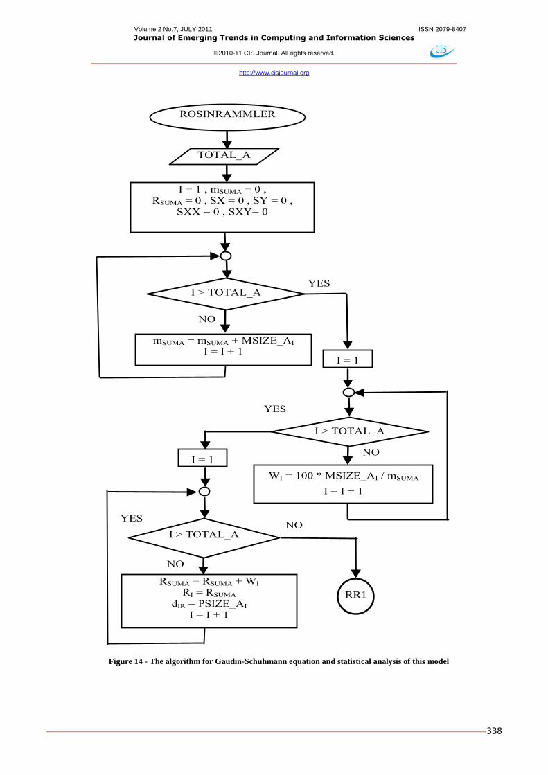
4. ALGORITHM FOR ROSIN-RAMMLER
LINEAR REGRESSION
On Figures 11, 12 and 13 is presents the
algorithm for determining the Rosin-Rammler equation
using linear regression. Firs step is to determine masses of
samples Wi in percentages which is calculated on masses
mi of size class. For this, is must calculated the total
weight of sample mSUMA as the sum of all partial class
fractions mi and then is performs the recalculation of the
masses of samples Wi in percentages. With this data, Ri is
calculated as the sum of the mass of samples Wi that
would be retained on the sieve diR.
Using converted original data, is calculated the
coefficients A, B for linear regression and values
D_PRIM, N_KOEF who representing the parameters d', n
of Rosin-Rammler equation obtained by linear regression
method. After that is calculated the coefficient of
determination and correlation coefficient for this model
(equation), as well as standard deviation, variance and
coefficient of variation for regression.
2^
yy
[%],100._
y
Vy
y
N , KOEF_A ,
KOEF_B
I = 1
SRED_Y = 0, SRAZ_Y = 0
I > N
NO
YRI = KOEF_A * XI + KOEF_B
SRAZ_Y = SRAZ_Y + (YI - YRI) ^ 2
SRED_Y = SRED_Y + YI
I = I + 1
YES
REGVARIA
SRED_Y = SRED_Y / N
RVARIA = SRAZ_Y / N
RDEVIA = RVARIA ^ 0.5
KVARIA = 100* RDEVIA / SRED_Y
RVARIA, RDEVIA,
KVARIA
END
Volume 2 No.7, JULY 2011 ISSN 2079-8407
Journal of Emerging Trends in Computing and Information Sciences
©2010-11 CIS Journal. All rights reserved.
http://www.cisjournal.org
338
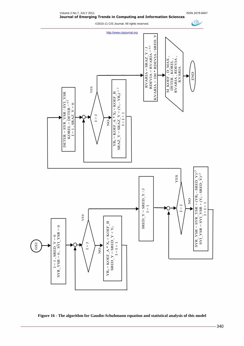
Figure 14 - The algorithm for Gaudin-Schuhmann equation and statistical analysis of this model
ROSINRAMMLER
TOTAL_A
I = 1 , mSUMA = 0 ,
RSUMA = 0 , SX = 0 , SY = 0 ,
SXX = 0 , SXY= 0
I > TOTAL_A
NO
mSUMA = mSUMA + MSIZE_AI
I = I + 1
YES
I = 1
I > TOTAL_A
NO
WI = 100 * MSIZE_AI / mSUMA
I = I + 1
YES
I = 1
I > TOTAL_A
NO
RSUMA = RSUMA + WI
RI = RSUMA
dIR = PSIZE_AI
I = I + 1
NO YES
RR1
Volume 2 No.7, JULY 2011 ISSN 2079-8407
Journal of Emerging Trends in Computing and Information Sciences
©2010-11 CIS Journal. All rights reserved.
http://www.cisjournal.org
339
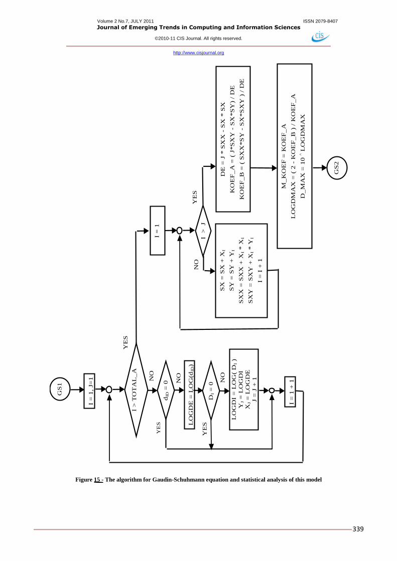
Figure 15 - The algorithm for Gaudin-Schuhmann equation and statistical analysis of this model
I =
1,
J=
1
I >
TO
TA
L_
A
NO
YE
S
dID
= 0
LO
GD
E =
LO
G(d
ID)
DI =
0 N
O
YE
S L
OG
DI
= L
OG
( D
I )
YJ =
LO
GD
I
XJ =
LO
GD
E
J =
J +
1
NO
YE
S
I =
1 +
1
GS
1
I =
1
I >
J
NO
Y
ES
DE
= J
* S
XX
- S
X *
SX
KO
EF
_A
= (
J*S
XY
- S
X*S
Y)
/ D
E
KO
EF
_B
= (
SX
X*S
Y -
SX
*S
XY
) /
DE
SX
= S
X +
XI
SY
= S
Y +
YI
SX
X =
SX
X +
XI * X
I
SX
Y =
SX
Y +
XI * Y
I
I =
I +
1
M_
KO
EF
= K
OE
F_
A
LO
GD
MA
X =
( 2
- K
OE
F_
B )
/ K
OE
F_
A
D_
MA
X =
10
^ L
OG
DM
AX
GS
2
Volume 2 No.7, JULY 2011 ISSN 2079-8407
Journal of Emerging Trends in Computing and Information Sciences
©2010-11 CIS Journal. All rights reserved.
http://www.cisjournal.org
340
Figure 16 - The algorithm for Gaudin-Schuhmann equation and statistical analysis of this model
I =
1 , S
RE
D_Y
= 0
SY
R_Y
SR
= 0
,
SY
I_Y
SR
= 0
I >
J
NO
YR
I =
KO
EF
_A
* X
I +
KO
EF
_B
SR
ED
_Y
= S
RE
D_Y
+ Y
I
I =
I +
1
YE
S
I >
J
NO
YR
I =
KO
EF
_A
* X
I +
KO
EF
_B
SR
AZ
_Y
= S
RA
Z_Y
+ (
YI -
YR
I) ^
2
I =
I +
1
YE
S RV
AR
IA =
SR
AZ
_Y
/ J
RD
EV
IA =
RV
AR
IA ^
0.5
KV
AR
IA =
100 *
RD
EV
IA /
SR
ED
_Y
M_K
OE
F ,
D_M
AX
,
DE
TE
R ,
KO
RE
L ,
RV
AR
IA ,
RD
EV
IA ,
KV
AR
IA
EN
D
DE
TE
R =
SY
R_Y
SR
/ S
YI_
YS
R
KO
RE
L =
DE
TE
R ^
0.5
I =
1 , S
RA
Z_Y
= 0
SR
ED
_Y
= S
RE
D_Y
/ J
I =
1
I >
J N
O
SY
R_Y
SR
= S
YR
_Y
SR
+ (
YR
I -
SR
ED
_Y
)^2
SY
I_Y
SR
= S
YI_
YS
R +
(Y
I -
SR
ED
_Y
)^2
I =
I +
1
YE
S
GS
2
Volume 2 No.7, JULY 2011 ISSN 2079-8407
Journal of Emerging Trends in Computing and Information Sciences
©2010-11 CIS Journal. All rights reserved.
http://www.cisjournal.org
341
CONCLUSION
This paper show the algorithms for determine the
Rosin-Rammler and Gaudin-Schuhmann equation of
particle size distribution using regresion analysis that
author of this paper used as starting point in the
construction of "UniModBase" information system [13,
14, 15].
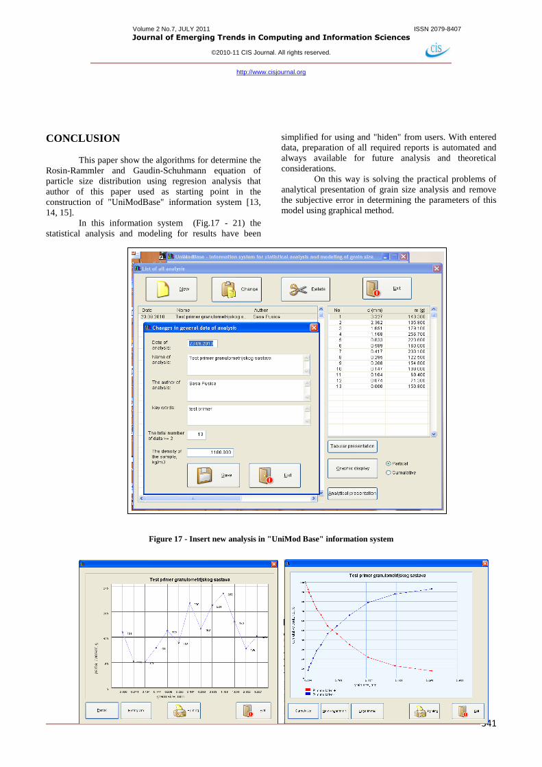
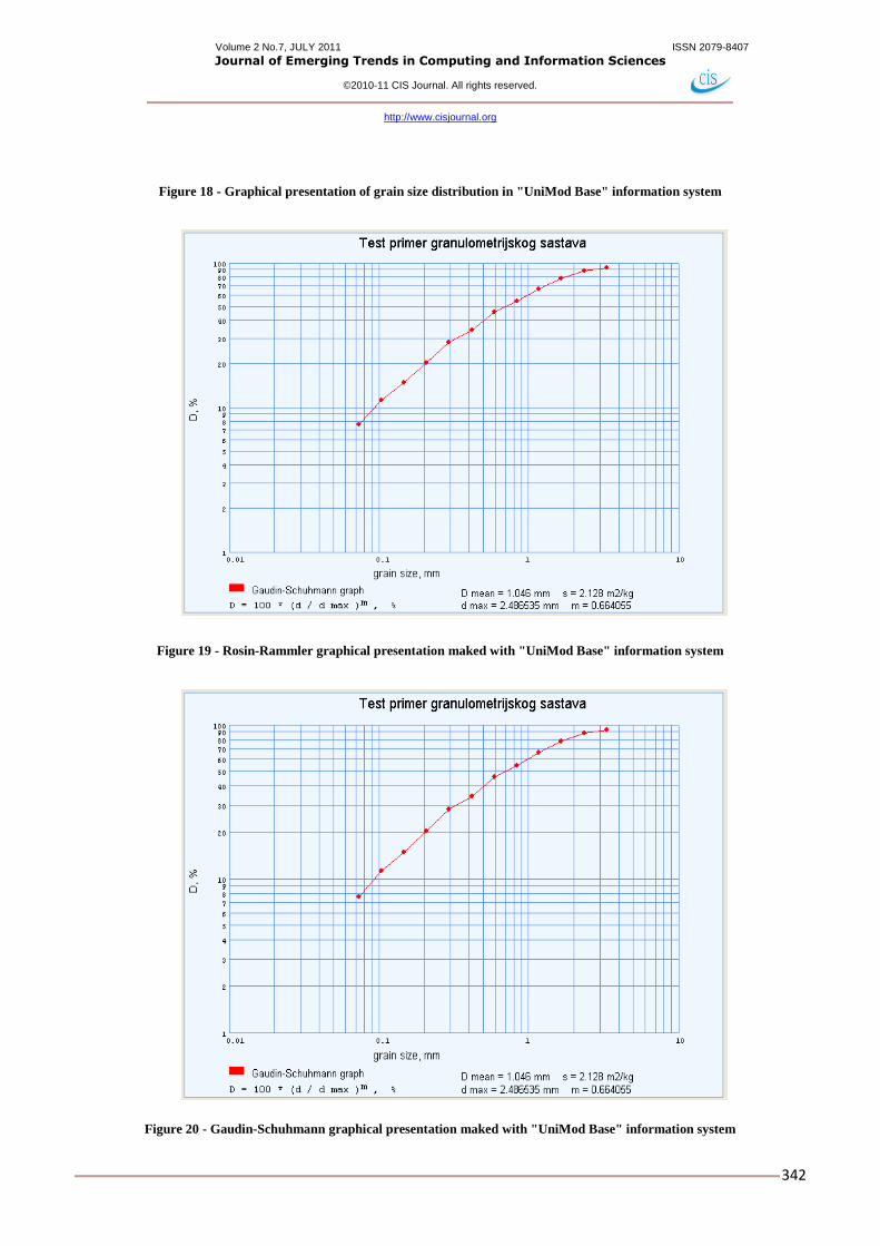
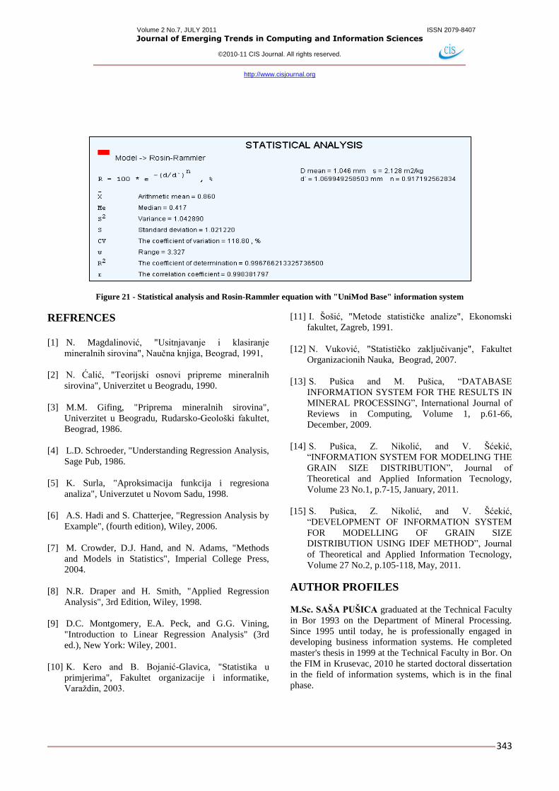
In this information system (Fig.17 - 21) the
statistical analysis and modeling for results have been
simplified for using and "hiden" from users. With entered
data, preparation of all required reports is automated and
always available for future analysis and theoretical
considerations.
On this way is solving the practical problems of
analytical presentation of grain size analysis and remove
the subjective error in determining the parameters of this
model using graphical method.
Figure 17 - Insert new analysis in "UniMod Base" information system
Volume 2 No.7, JULY 2011 ISSN 2079-8407
Journal of Emerging Trends in Computing and Information Sciences
©2010-11 CIS Journal. All rights reserved.
http://www.cisjournal.org
342
Figure 18 - Graphical presentation of grain size distribution in "UniMod Base" information system
Figure 19 - Rosin-Rammler graphical presentation maked with "UniMod Base" information system
Figure 20 - Gaudin-Schuhmann graphical presentation maked with "UniMod Base" information system
Volume 2 No.7, JULY 2011 ISSN 2079-8407
Journal of Emerging Trends in Computing and Information Sciences
©2010-11 CIS Journal. All rights reserved.
http://www.cisjournal.org
343
Figure 21 - Statistical analysis and Rosin-Rammler equation with "UniMod Base" information system
REFRENCES
[1] N. Magdalinović, "Usitnjavanje i klasiranje
mineralnih sirovina", Naučna knjiga, Beograd, 1991,
[2] N. Ćalić, "Teorijski osnovi pripreme mineralnih
sirovina", Univerzitet u Beogradu, 1990.
[3] M.M. Gifing, "Priprema mineralnih sirovina",
Univerzitet u Beogradu, Rudarsko-Geološki fakultet,
Beograd, 1986.
[4] L.D. Schroeder, "Understanding Regression Analysis,
Sage Pub, 1986.
[5] K. Surla, "Aproksimacija funkcija i regresiona
analiza", Univerzutet u Novom Sadu, 1998.
[6] A.S. Hadi and S. Chatterjee, "Regression Analysis by
Example", (fourth edition), Wiley, 2006.
[7] M. Crowder, D.J. Hand, and N. Adams, "Methods
and Models in Statistics", Imperial College Press,
2004.
[8] N.R. Draper and H. Smith, "Applied Regression
Analysis", 3rd Edition, Wiley, 1998.
[9] D.C. Montgomery, E.A. Peck, and G.G. Vining,
"Introduction to Linear Regression Analysis" (3rd
ed.), New York: Wiley, 2001.
[10] K. Kero and B. Bojanić-Glavica, "Statistika u
primjerima", Fakultet organizacije i informatike,
Varaždin, 2003.
[11] I. Šošić, "Metode statističke analize", Ekonomski
fakultet, Zagreb, 1991.
[12] N. Vuković, "Statističko zaključivanje", Fakultet
Organizacionih Nauka, Beograd, 2007.
[13] S. Pušica and М. Pušica, “DATABASE
INFORMATION SYSTEM FOR THE RESULTS IN
MINERAL PROCESSING”, International Journal of
Reviews in Computing, Volume 1, p.61-66,
December, 2009.
[14] S. Pušica, Z. Nikolić, and V. Šćekić,
“INFORMATION SYSTEM FOR MODELING THE
GRAIN SIZE DISTRIBUTION”, Journal of
Theoretical and Applied Information Tecnology,
Volume 23 No.1, p.7-15, January, 2011.
[15] S. Pušica, Z. Nikolić, and V. Šćekić,
“DEVELOPMENT OF INFORMATION SYSTEM
FOR MODELLING OF GRAIN SIZE
DISTRIBUTION USING IDEF METHOD”, Journal
of Theoretical and Applied Information Tecnology,
Volume 27 No.2, p.105-118, May, 2011.
AUTHOR PROFILES
M.Sc. SAŠA PUŠICA graduated at the Technical Faculty
in Bor 1993 on the Department of Mineral Processing.
Since 1995 until today, he is professionally engaged in
developing business information systems. He completed
master's thesis in 1999 at the Technical Faculty in Bor. On
the FIM in Krusevac, 2010 he started doctoral dissertation
in the field of information systems, which is in the final
phase.