Contents lists available at SciVerse ScienceDirect

Journal of Financial Economics

Journal of Financial Economics 109 (2013) 707–733

0304-40http://d

☆ WeSchwerDufresnFlemingLund, FaScalliet,ConfereMathemworkshTargetinand RisQuantittives CoFinanciaUniversDenmarZurich,versityexcellenport bySwiss N

n CorrE-m

journal homepage: www.elsevier.com/locate/jfec

The term structure of interbank risk$

Damir Filipović, Anders B. Trolle n

Ecole Polytechnique Fédérale de Lausanne and Swiss Finance Institute, Switzerland

a r t i c l e i n f o

Article history:Received 5 April 2012Received in revised form30 October 2012Accepted 26 November 2012Available online 2 May 2013

JEL classifications:E43G01G12

Keywords:Interbank riskLIBORInterest rate swapsDefault riskLiquidity

5X/$ - see front matter & 2013 Elsevier B.V.x.doi.org/10.1016/j.jfineco.2013.03.014

are grateful for the comments and advict, and the referee, Caio Almeida. We alsoe, Darrell Duffie, Rudiger Fahlenbrach, Peter, Masaaki Fujii, Joao Gomes, Holger Kraft,bio Mercurio, Erwan Morellec, Claus Munk, AMarco Taboga, Christian Upper, and seminance on Liquidity and Credit Risk in Freiburgatical Modeling of Systemic Risk in Paris,op, the 2011 Credit Risk Evaluation Designg (CREDIT) conference in Venice, the 2011k Management (FINRISK) research day, theative Risk Management in Oberwolfach, thenference in Barcelona, the 2013 Federal Rel Markets and Institutions in San Diego,ity in Frankfurt, University of Lisbon, Unk, University of St. Gallen, University ofand the Ecole Polytechnique Fédérale de Lof Lausanne brownbag for comments. Sht research assistance. We gratefully acknowNCCR (National Centre of Competence in Resational Science Foundation.esponding author.ail address: anders.trolle@epfl.ch (A.B. Trolle

a b s t r a c t

We infer a term structure of interbank risk from spreads between rates on interest rateswaps indexed to the London Interbank Offered Rate (LIBOR) and overnight indexedswaps. We develop a tractable model of interbank risk to decompose the term structureinto default and non-default (liquidity) components. From August 2007 to January 2011,the fraction of total interbank risk due to default risk, on average, increases with maturity.At short maturities, the non-default component is important in the first half of the sampleperiod and is correlated with measures of funding and market liquidity. The model alsoprovides a framework for pricing, hedging, and risk management of interest rate swaps inthe presence of significant basis risk.

& 2013 Elsevier B.V. All rights reserved.

All rights reserved.

e of the editor, Billthank Pierre Collin-Feldhutter, MichaelDavid Lando, Jesperlberto Plazzi, Olivierr participants at the, the Conference onthe 2011 Chemnitzed for InstitutionalFinancial Valuation2012 workshop on2012 Global Deriva-serve Conference onETH Zurich, Goetheiversity of SouthernTokyo, University ofausanne (EPFL)-Uni-adi Akiki providedledge financial sup-earch) FINRISK of the

).

1. Introduction

Interbank risk, as defined in this paper, is the risk ofdirect or indirect loss resulting from lending in the inter-bank money market. The recent financial crisis has high-lighted the implications of such risk for financial marketsand economic growth. While existing studies provideimportant insights on the determinants of short-terminterbank risk, very little is known about the term struc-ture of interbank risk. We provide a comprehensiveanalysis of this topic. First, we develop a tractable modelof the term structure of interbank risk, connecting theinterbank money market to the interest rate swap (IRS)and credit default swap (CDS) markets. Second, we applythe model to analyze interbank risk since the onset of thefinancial crisis, decomposing the term structure of inter-bank risk into default and non-default (liquidity) compo-nents, and study their associated risk premiums.

We follow most existing studies by measuring inter-bank risk as the spread between a London InterbankOffered Rate (LIBOR) and the rate on a maturity-matchedovernight indexed swap (OIS). The former is a reference

D. Filipović, A.B. Trolle / Journal of Financial Economics 109 (2013) 707–733708

rate for unsecured interbank borrowing and lending, andthe latter is a common risk-free rate proxy. We show thatthe spread between the fixed rate on an IRS with floating-leg payments indexed to, say, three-month LIBOR and anOIS of the same maturity reflects risk-neutral expectationsabout future three-month LIBOR-OIS spreads and, there-fore, future three-month interbank risk. This allows us toinfer a term structure of interbank risk from IRS-OISspreads of different maturities.

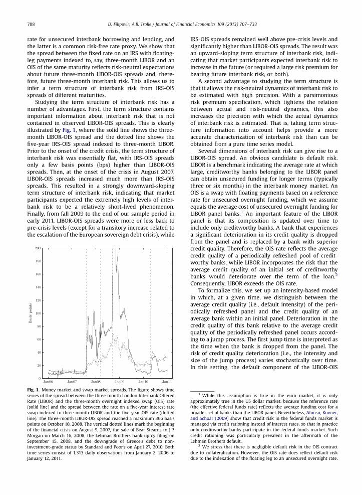
Studying the term structure of interbank risk has anumber of advantages. First, the term structure containsimportant information about interbank risk that is notcontained in observed LIBOR-OIS spreads. This is clearlyillustrated by Fig. 1, where the solid line shows the three-month LIBOR-OIS spread and the dotted line shows thefive-year IRS-OIS spread indexed to three-month LIBOR.Prior to the onset of the credit crisis, the term structure ofinterbank risk was essentially flat, with IRS-OIS spreadsonly a few basis points (bps) higher than LIBOR-OISspreads. Then, at the onset of the crisis in August 2007,LIBOR-OIS spreads increased much more than IRS-OISspreads. This resulted in a strongly downward-slopingterm structure of interbank risk, indicating that marketparticipants expected the extremely high levels of inter-bank risk to be a relatively short-lived phenomenon.Finally, from fall 2009 to the end of our sample period inearly 2011, LIBOR-OIS spreads were more or less back topre-crisis levels (except for a transitory increase related tothe escalation of the European sovereign debt crisis), while

Fig. 1. Money market and swap market spreads. The figure shows timeseries of the spread between the three-month London Interbank OfferedRate (LIBOR) and the three-month overnight indexed swap (OIS) rate(solid line) and the spread between the rate on a five-year interest rateswap indexed to three-month LIBOR and the five-year OIS rate (dottedline). The three-month LIBOR-OIS spread reached a maximum 366 basispoints on October 10, 2008. The vertical dotted lines mark the beginningof the financial crisis on August 9, 2007, the sale of Bear Stearns to J.P.Morgan on March 16, 2008, the Lehman Brothers bankruptcy filing onSeptember 15, 2008, and the downgrade of Greece's debt to non-investment-grade status by Standard and Poor's on April 27, 2010. Bothtime series consist of 1,313 daily observations from January 2, 2006 toJanuary 12, 2011.

IRS-OIS spreads remained well above pre-crisis levels andsignificantly higher than LIBOR-OIS spreads. The result wasan upward-sloping term structure of interbank risk, indi-cating that market participants expected interbank risk toincrease in the future (or required a large risk premium forbearing future interbank risk, or both).

A second advantage to studying the term structure isthat it allows the risk-neutral dynamics of interbank risk tobe estimated with high precision. With a parsimoniousrisk premium specification, which tightens the relationbetween actual and risk-neutral dynamics, this alsoincreases the precision with which the actual dynamicsof interbank risk is estimated. That is, taking term struc-ture information into account helps provide a moreaccurate characterization of interbank risk than can beobtained from a pure time series model.

Several dimensions of interbank risk can give rise to aLIBOR-OIS spread. An obvious candidate is default risk.LIBOR is a benchmark indicating the average rate at whichlarge, creditworthy banks belonging to the LIBOR panelcan obtain unsecured funding for longer terms (typicallythree or six months) in the interbank money market. AnOIS is a swap with floating payments based on a referencerate for unsecured overnight funding, which we assumeequals the average cost of unsecured overnight funding forLIBOR panel banks.1 An important feature of the LIBORpanel is that its composition is updated over time toinclude only creditworthy banks. A bank that experiencesa significant deterioration in its credit quality is droppedfrom the panel and is replaced by a bank with superiorcredit quality. Therefore, the OIS rate reflects the averagecredit quality of a periodically refreshed pool of credit-worthy banks, while LIBOR incorporates the risk that theaverage credit quality of an initial set of creditworthybanks would deteriorate over the term of the loan.2

Consequently, LIBOR exceeds the OIS rate.To formalize this, we set up an intensity-based model

in which, at a given time, we distinguish between theaverage credit quality (i.e., default intensity) of the peri-odically refreshed panel and the credit quality of anaverage bank within an initial panel. Deterioration in thecredit quality of this bank relative to the average creditquality of the periodically refreshed panel occurs accord-ing to a jump process. The first jump time is interpreted asthe time when the bank is dropped from the panel. Therisk of credit quality deterioration (i.e., the intensity andsize of the jump process) varies stochastically over time.In this setting, the default component of the LIBOR-OIS

1 While this assumption is true in the euro market, it is onlyapproximately true in the US dollar market, because the reference rate(the effective federal funds rate) reflects the average funding cost for abroader set of banks than the LIBOR panel. Nevertheless, Afonso, Kovner,and Schoar (2009) show that credit risk in the federal funds market ismanaged via credit rationing instead of interest rates, so that in practiceonly creditworthy banks participate in the federal funds market. Suchcredit rationing was particularly prevalent in the aftermath of theLehman Brothers default.

2 We stress that there is negligible default risk in the OIS contractdue to collateralization. However, the OIS rate does reflect default riskdue to the indexation of the floating leg to an unsecured overnight rate.

5 The issue is whether certain banks strategically manipulated theirLIBOR quotes to signal information about their credit quality or liquidityneeds or to influence LIBOR to benefit positions in LIBOR-linkedinstruments.

6 A recent study by Kuo, Skeie, and Vickery (2012) compares LIBOR

D. Filipović, A.B. Trolle / Journal of Financial Economics 109 (2013) 707–733 709

spread is driven by the expected rate of credit qualitydeterioration of an average bank within the initial panel.

A LIBOR-OIS spread could also arise due to factors notdirectly related to default risk, primarily liquidity. Thereare several reasons that liquidity in the market for inter-bank funding beyond the ultra-short term can deteriorate.For instance, banks could refrain from lending longer termfor precautionary reasons, if they fear adverse shocks totheir own funding situation, or for speculative reasons, ifthey anticipate possible fire sales of assets by otherfinancial institutions.3 Instead of modeling these mechan-isms directly, we posit a residual factor that captures thecomponent of the LIBOR-OIS spread that is not due todefault risk. To the extent that liquidity effects are corre-lated with default risk, the residual factor captures the partof liquidity that is unspanned by default risk.

The default and non-default components in an IRS-OISspread reflect risk-neutral expectations about the defaultand non-default components in future LIBOR-OIS spreads.To separate the two components, we use information fromthe credit default swap market. At each observation date,we construct a CDS spread term structure for an averagepanel bank as a composite of the CDS spread termstructures for the individual panel banks. The compositeCDS spread term structure allows us to estimate the risk-neutral process for credit quality deterioration of anaverage panel bank and then to infer the default compo-nent in LIBOR-OIS spreads. Importantly, the potential forrefreshment of the LIBOR panel combined with the risk ofcredit quality deterioration makes the default componentin an IRS-OIS spread lower than the default risk reflectedby a maturity-matched CDS spread.4

Our model is set within a general affine framework.Depending on the specification, two factors drive OIS rates,one or two factors drive the default component of LIBOR-OIS spreads (i.e., the risk of credit quality deterioration),and one or two factors drive the non-default component ofLIBOR-OIS spreads. The model is highly tractable withanalytical expressions for LIBOR, OIS, IRS, and CDS.In valuing swap contracts, we match as closely as possiblecurrent market practice regarding collateralization.

We apply the model to study interbank risk from theonset of the financial crisis in August 2007 until January2011. We utilize a panel data set consisting of termstructures of OIS rates, IRS-OIS spreads indexed to three-month and six-month LIBOR, and CDS spreads—all withmaturities up to ten years. The model is estimated bymaximum likelihood in conjunctionwith the Kalman filter.

3 The precautionary motive for cash hoarding is modeled by Allen,Carletti, and Gale (2009) and Acharya and Skeie (2011). The speculativemotive for cash hoarding is modeled by Acharya, Gromb, and Yorulmazer(2012), Acharya, Shin, and Yorulmazer (2011), and Diamond and Rajan(2011). A recent model by Gale and Yorulmazer (2011) features both theprecautionary and speculative motive for cash holdings.

4 The main component of a composite CDS spread is the expectedcredit quality deterioration, over the maturity of the CDS contract, of anaverage bank within the current panel. In contrast, the default compo-nent of an IRS-OIS spread reflects a series of expected short-term creditquality deteriorations, from each LIBOR fixing date to the next, of averagebanks within future refreshed panels.

We conduct a specification analysis, which shows that aspecification with two factors driving OIS rates, two factorsdriving the default component of LIBOR-OIS spreads, andone factor driving the non-default component of LIBOR-OIS spreads has a satisfactory fit to the data, while beingfairly parsimonious. We then use this specification todecompose the term structure of interbank risk intodefault and non-default components. We find that, onaverage, the fraction of total interbank risk due to defaultrisk increases with maturity. At the short end of the termstructure, the non-default component is important in thefirst half of the sample period. At longer maturities, thedefault component is the dominant driver of interbank riskthroughout the sample period.

To what extent are our results affected by possiblestrategic behavior by certain LIBOR contributors duringparts of the sample period?5 First, the procedure forcomputing LIBOR should limit the impact of strategicbehavior.6 Second, even to the extent that LIBOR wereaffected, this is unlikely to impact our results, becauseinterbank risk is primarily inferred from the cross sectionof swap rates, which are determined in highly competitivemarkets. Instead, idiosyncratic variation in LIBOR ratesshow up as a pricing error in our Kalman filter setting.Nonetheless, to verify the robustness of our results, wereestimate the model using only swap rates and no LIBORrates but find no significant changes to the results. Thisrobustness check can be found in the online Appendix.

To understand the determinants of the non-defaultcomponent of interbank risk, we relate the residual factorto a number of proxies for funding liquidity and marketliquidity, which tend to be highly intertwined(Brunnermeier and Pedersen, 2009). Specifically, weregress the residual factor on the components of theliquidity proxies, which are unspanned by interbankdefault risk.7 The R2 reaches 64% in a multivariate regres-sion specification, strongly suggesting that the non-defaultcomponent of interbank risk largely captures liquidityeffects not spanned by default risk.

We also provide tentative evidence on the pricing ofinterbank risk in the interest rate swap market. We findthat swap market participants require compensation for

with rates on actual interbank borrowing by LIBOR panel banks at theone-month, three-month, and six-month maturities during the crisisperiod. They find that LIBOR is a reasonably accurate reflection of theaverage unsecured funding costs of LIBOR panel banks in the interbankmoney market. The main exception is the two-week period following theLehman Brothers default, when LIBOR underestimates funding costs byabout 20 bps. The difference between quoted and transacted rates,however, is only marginally statistically significant and should be put inrelation to the extremely elevated LIBOR-OIS spreads during this period,as shown in Fig. 1. Going forward, the proposals for greater regulatoryoversight and increased transparency set out in the Wheatley (2012)report should diminish concerns about the integrity of LIBOR.

7 For each liquidity measure, the component that is unspanned byinterbank default risk is given by the residual from a regression of theliquidity measure on the first two principal components of the compositeCDS term structure.

9 CS use the Treasury curve instead of the OIS curve as the referencecurve. In their model, IRS-Treasury spreads do vary over time, becausethe default intensity of the periodically refreshed panel is stochastic.

10 Our paper is also related to Liu, Longstaff, and Mandell (2006),Johannes and Sundaresan (2007), and Feldhutter and Lando (2008), whostudy the term structure of IRS-Treasury spreads. Feldhutter and Lando

D. Filipović, A.B. Trolle / Journal of Financial Economics 109 (2013) 707–733710

exposure to variation in interbank default risk, while weare not able to reliably estimate the compensationrequired for exposure to the residual factor. This impliesthat in the first part of the sample period, when the non-default component dominates, the overall compensationfor variation in interbank risk is low. In contrast, in thesecond part of the sample period, when the defaultcomponent dominates, the overall compensation for var-iation in interbank risk is significant. For instance, theinstantaneous Sharpe ratio on a strategy of being long thefive-year IRS-OIS spread indexed to three-month LIBOR isestimated to have averaged 0.35 from early 2009 to theend of the sample period.

Throughout, we also report results for the euro (EUR)market. Not only does this serve as a robustness check, butthis market is also interesting in its own right. First, byseveral measures, the market is even larger than the USdollar (USD) market. Second, the structure of the EURmarket is such that the reference overnight rate in an OISexactly matches the average cost of unsecured overnightfunding of EURIBOR (European Interbank Offered Rate, theEUR equivalent of LIBOR) panel banks, providing a check ofthis assumption. And, third, the main shocks to theinterbank money market in the second half of the sampleperiod emanated from the Eurozone with its sovereigndebt crisis. Indeed, we find that interbank risk in the EURmarket is generally higher than interbank risk in the USDmarket during the second half of the sample period, andthat the opposite is true during the first half. Nevertheless,results on the decomposition of interbank risk, the driversof the residual factor, and the risk compensation in theswap market are similar to the USD market.

As a plausibility check of the model-based decomposi-tion, we consider a simple regression-based decomposi-tion in which each interest rate spread (LIBOR-OIS or IRS-OIS) is regressed on a maturity-matched CDS spread.8 Thisregression-based decomposition gives results that arequalitatively similar to the model-based decomposition.

In addition to providing insights into the dynamics anddeterminants of interbank risk, the model should be usefulfor pricing, hedging, and risk management in the interestrate swap market. Since the onset of the credit crisis,market participants have been exposed to significant basisrisk: Swap cash flows are indexed to LIBOR but, because ofcollateral agreements, are discounted using rates inferredfrom the OIS market. Furthermore, swap portfolios at mostfinancial institutions are composed of swap contractsindexed to LIBOR rates of various maturities, creatinganother layer of basis risk. Our model provides a frame-work for managing overall interest rate risk and thesebasis risks in an integrated way. From a regulatory stand-point, the model could be useful for determining the rightdiscount curve for the valuation of long-term insuranceliabilities, where discount factors are typically allowed to

8 The coefficient on the CDS spread is always less than one anddecreases with swap maturity. This is consistent with the observationthat the default component in an IRS-OIS spread is lower than thematurity-matched CDS spread, with the difference increasing in swapmaturity.

include a liquidity component but not a default riskcomponent.

Our paper is most closely related to Collin-Dufresneand Solnik (2001, henceforth CS), who study the termstructure of spreads between yields on corporate bondsissued by LIBOR banks and IRS rates. In their model, aspread arises because bond yields reflect the possibility ofdeterioration in the credit quality of current LIBOR banksrelative to that of future LIBOR banks. A similar mechanismis present in our model. However, several importantdifferences exist between CS and our paper. First, in theCS model, LIBOR reflects only default risk; in our model,LIBOR reflects both default and non-default (liquidity) risk,which allows a decomposition of interbank risk. Second,CS assume a constant intensity of credit quality deteriora-tion, causing the implicit IRS-OIS spread term structures tobe virtually flat and constant across time.9 In contrast, weallow the intensity of credit quality deterioration to varystochastically, which produces rich dynamics of the defaultcomponent of spreads (with additional spread dynamicscoming from the non-default component). Third, in the CSmodel, shocks to credit quality are permanent, while weallow for gradual improvement in credit quality followinga shock, further improving the fit of the model. Fourth, inthe empirical analysis we use CDSs instead of corporatebonds and OISs instead of Treasuries. Corporate bonds andTreasuries were heavily affected by liquidity and flight-to-quality issues during the crisis. By considering only swapcontracts, we expect liquidity to be less of an issue and tobe more uniform across instruments leading to a cleandecomposition of the term structure of interbank risk.10

A number of papers have analyzed the three-monthLIBOR-OIS spread and attempted to decompose it intodefault and liquidity components. These papers includeSchwartz (2010), Taylor and Williams (2009), McAndrews,Sarkar, and Wang (2008), Michaud and Upper (2008), andEisenschmidt and Tapking (2009). They all study the earlyphase of the financial crisis before the collapse of LehmanBrothers and find, with the exception of Taylor andWilliams (2009), that liquidity was a key driver of inter-bank risk during this period. We find a similar result forthe short end of the term structure of interbank risk.However, at longer maturities, default risk appears to havebeen the dominant driver even during the early phase ofthe financial crisis, underscoring the importance of takingthe entire term structure into account when analyzinginterbank risk.11

(2008) allow for a non-default component in the spread between LIBORand the (unobservable) risk-free rate, which they argue is related tohedging flows in the IRS market during their pre-crisis sample period.

11 Smith (2010) studies LIBOR-OIS spreads of maturities up to 12months within a dynamic term structure model and attributes most ofthe variation in spreads to variation in risk premiums. A somewhatproblematic aspect of her analysis is that the default component ofLIBOR-OIS spreads is identified by the spread between LIBOR and repo

12 After the end of our sample period, the USD LIBOR panel wasexpanded to 20 banks and the EURIBOR panel was expanded to 44 banks.

13 Participants in the federal funds market are those with accounts atFederal Reserve banks, which include US depository institutions, US

D. Filipović, A.B. Trolle / Journal of Financial Economics 109 (2013) 707–733 711

Several papers including Bianchetti (2009), Fujii,Shimada, and Takahashi (2009), Henrard (2009), andMercurio (2009, 2010) have developed pricing models forinterest rate derivatives that take the stochastic IRS-OISspread into account. These are highly reduced-form mod-els in that swap spreads indexed to different LIBOR ratesare modeled independently of each other and are notdecomposed into different components. In contrast, weprovide a unified model of all such spreads, making itpossible to aggregate the risk of large swap portfolios andanalyze their underlying determinants.

The rest of the paper is organized as follows: Section 2describes the market instruments. Section 3 describes themodel of the term structure of interbank risk. Section 4discusses the data and the estimation approach. Section 5presents the results. Section 6 concludes, and severalappendices contain pricing formulas, proofs, and detailson the estimation. An online Appendix contains additionalmaterial, including a large number of robustness checksshowing that the results hold true for alternative modelparameterizations and measures of interbank default risk.

2. Market instruments

We describe the market instruments that we use in thepaper. We first consider the basic reference rates and thena variety of swap contracts that are indexed to thesereference rates.

2.1. Reference rates

A large number of fixed income contracts are tied to aninterbank offered rate. The main reference rate in the USD-denominated fixed income market is USD LIBOR. In theEUR-denominated fixed income market it is EURIBOR(there also exists a EUR LIBOR, although this rate has notreceived the same benchmark status as EURIBOR). BothLIBOR and EURIBOR are trimmed averages of rates sub-mitted by sets of banks. In the case of LIBOR, eachcontributor bank bases its submission on the question:“At what rate could you borrow funds, were you to do soby asking for and then accepting interbank offers in areasonable market size?”. In the case of EURIBOR, thewording is slightly different and each contributor banksubmits “the rates at which euro interbank term depositsare being offered within the Eurozone by one prime bankto another”. Therefore, LIBOR is an average of the rates atwhich banks believe they can obtain unsecured funding,and EURIBOR is an average of the rates at which banksbelieve a prime bank can obtain unsecured funding. Thissubtle difference becomes important when quantifying thedegree of default risk inherent in the two rates. Both ratesare quoted for a range of terms, with three and six monthsbeing the most important and most widely followed. Inthe following, we let L t; Tð Þ denote the T−tð Þ-maturityLIBOR or EURIBOR rate that fixes at time t.

(footnote continued)rates, which clearly contains a significant liquidity component duringmuch of the period.

For both LIBOR and EURIBOR, contributor banks areselected based on their credit quality and the scale of theirmarket activities. During our sample period, the LIBORpanel consisted of 16 banks and the EURIBOR panel wassignificantly larger, consisting of 42 banks.12 An importantfeature of both panels is that they are reviewed andrevised periodically. A bank that experiences a significantdeterioration in its credit quality (or its market share, orboth) is dropped from the panel and is replaced by a bankwith superior credit quality.

An increasing number of fixed income contracts aretied to an index of overnight rates. In the USD market, thebenchmark is the effective federal funds (FF) rate, which isa transaction-weighted average of the rates on overnightunsecured loans of reserve balances held at the FederalReserve that banks make to one another. In the EURmarket, the benchmark is the Euro Overnight IndexAverage (EONIA) rate, computed as a transaction-weighted average of the rates on all overnight unsecuredloans in the interbank money market initiated by EURIBORpanel banks. Therefore, in the EUR market, the benchmarkovernight rate reflects the average cost of unsecuredovernight funding of panel banks. We assume that thesame holds for the USD market, although the set of banksfrom which the effective federal funds rate is computeddoes not exactly match the LIBOR panel.13

For the sake of convenience, we use “LIBOR” as ageneric term for an interbank offered rate, comprisingboth LIBOR and EURIBOR, whenever there is no ambiguity.

2.2. Pricing collateralized contracts

Swap contracts between major financial institutions arevirtually always collateralized to the extent that counter-party risk is negligible.14 In this subsection, we provide thegeneric pricing formula of collateralized cash flows thatwe use to price swap contracts. Similar formulas have beenderived in various contexts by Johannes and Sundaresan(2007), Fujii, Shimada, and Takahashi (2009), and Piterbarg(2010). Consider a contract with a contractual nominalcash flow X at maturity T. Its present value at toT isdenoted by V(t). We assume that the two parties in thecontract agree on posting cash-collateral on a continuousmarking-to-market basis. We also assume that, at any timetoT , the posted amount of collateral equals 100% of thecontract's present value V(t). The receiver of the collateralcan invest it at the risk-free rate r(t) and has to pay anagreed rate rc(t) to the poster of collateral. The present

branches of foreign banks, and government-sponsored enterprises.14 Even in the absence of collateralization, counterparty risk usually

has only a very small effect on the valuation of swap contracts; see, e.g.,Duffie and Huang (1996). This led to the approach to interest rate swappricing in Duffie and Singleton (1997).

D. Filipović, A.B. Trolle / Journal of Financial Economics 109 (2013) 707–733712

value thus satisfies the integral equation

V tð Þ ¼ EQt e−R T

tr sð Þ dsX þ

Z T

te−R u

tr sð Þ ds r uð Þ−rc uð Þð ÞV uð Þ du

� �;

ð1Þwhere, throughout, we assume a filtered probability spaceΩ;F ;F t ;Qð Þ, where Q is a risk-neutral pricing measure,and EQ

t ≡EQ �jF t½ � denotes conditional expectation under Q.

Appendix A shows that this implies the pricing formula

V tð Þ ¼ EQt e−R T

trc sð Þ dsX

� �: ð2Þ

For X¼1, we obtain the price of a collateralized zero-coupon bond

Pc t; Tð Þ ¼ EQt e−R T

trc sð Þ ds

� �: ð3Þ

In the sequel, we assume that the collateral rate rc(t) isequal to an instantaneous proxy L t; tð Þ of the overnightrate, which we define as

rc tð Þ ¼ L t; tð Þ ¼ limT-t

L t; Tð Þ: ð4Þ

In reality, best practice among major financial institu-tions is daily marking-to-market and adjustment of col-lateral. Furthermore, cash collateral is the most popularform of collateral, because it is free from the issuesassociated with rehypothecation and allows for fastersettlement times. Finally, FF and EONIA are typically thecontractual interest rates earned by cash collateral in theUSD and EUR markets, respectively. The assumptions wemake, therefore, closely approximate current marketreality.15

2.3. Interest rate swaps

In a regular interest rate swap, counterparties exchangea stream of fixed-rate payments for a stream of floating-rate payments indexed to LIBOR of a particular maturity.More specifically, consider two discrete tenor structures:

t ¼ t0ot1o⋯otN ¼ T ð5Þ

and

t ¼ T0oT1o⋯oTn ¼ T ; ð6Þ

and let δ¼ ti−ti−1 and Δ¼ Ti−Ti−1 denote the lengthsbetween tenor dates, with δoΔ.16 At every time ti, i¼1,…,N, one party pays δL ti−1; tið Þ, and at every time Ti, i¼1,…,n, the other party pays ΔK , where K denotes the fixed rateon the swap. The swap rate, IRSδ;Δ t; Tð Þ, is the value of Kthat makes the IRS value equal to zero at inception and is

15 International Swaps and Derivatives Association (2010) is adetailed survey of current market practice. Further evidence for thepricing formula given in this subsection is provided by Whittall (2010),who reports that the main clearinghouse of swap contracts now usesdiscount factors extracted from the OIS term structure to value collater-alized swap cash flows.

16 In practice, the length between dates varies slightly depending onthe day-count convention. To simplify notation, we suppress thisdependence.

given by

IRSδ;Δ t; Tð Þ ¼∑N

i ¼ 1EQt e−

R tit

rc sð Þ dsδL ti−1; tið Þ� �∑n

i ¼ 1ΔPc t; Tið Þ : ð7Þ

In the USD market, the benchmark IRS pays three-monthLIBOR floating versus six-month fixed. In the EUR market,the benchmark IRS pays six-month EURIBOR floatingversus one-year fixed. Rates on IRS indexed to LIBOR ofother maturities are obtained via basis swaps (BS).

2.4. Basis swaps

In a basis swap, counterparties exchange two streamsof floating-rate payments indexed to LIBOR of differentmaturities, plus a stream of fixed payments. The quotationconvention for basis swaps differs across brokers andacross markets, and it could also have changed over time.However, as demonstrated in the online Appendix, thedifferences between the conventions are negligible. Con-sider a basis swap in which one party pays the δ1-maturityLIBOR and the other party pays the δ2-maturity LIBOR withδ1oδ2. We use the quotation convention in which thebasis swap rate, BSδ1 ;δ2 t; Tð Þ, is given as the differencebetween the fixed rates on two IRS indexed to δ2- andδ1-maturity LIBOR, respectively. That is,

BSδ1 ;δ2 t; Tð Þ ¼ IRSδ2 ;Δ t; Tð Þ−IRSδ1 ;Δ t; Tð Þ: ð8Þ

This convention has the advantage that rates on non-benchmark IRS are very easily obtained via basis swaps.

2.5. Overnight indexed swaps

In an overnight indexed swap, counterparties exchangea stream of fixed-rate payments for a stream of floating-rate payments indexed to a compounded overnight rate(FF or EONIA). In contrast to an IRS, an OIS typically hasfixed-rate payments and floating-rate payments occurringat the same frequency. Consider the tenor structure givenin (6) with Δ¼ Ti−Ti−1. At every time Ti, i¼1,…,n, one partypays ΔK and the other party pays ΔL Ti−1; Tið Þ, whereL Ti−1; Tið Þ is the compounded overnight rate for the periodTi−1; Ti½ �. This rate is given by

L Ti−1; Tið Þ ¼ 1Δ

∏Ki

j ¼ 11þ tj−tj−1

� �L tj−1; tj� �� �

−1Þ; ð9Þ

where Ti−1 ¼ t0ot1o⋯otKi¼ Ti denotes the partition of

the period Ti−1; Ti½ � into Ki business days, and L tj−1; tj� �

denotes the respective overnight rate. As in Andersen andPiterbarg (2010, Subsection 5.5), we approximate simpleby continuous compounding and the overnight rate by theinstantaneous rate L t; tð Þ given in Eq. (4), in which caseL Ti−1; Tið Þ becomes

L Ti−1; Tið Þ ¼ 1Δ

eR TiTi−1

rc sð Þ ds−1:

!ð10Þ

D. Filipović, A.B. Trolle / Journal of Financial Economics 109 (2013) 707–733 713

The OIS rate is the value of K that makes the OIS valueequal to zero at inception and is given by

OIS t; Tð Þ ¼∑n

i ¼ 1EQt e−

R Tit

rc sð Þ dsΔL Ti−1; Tið Þ� �∑n

i ¼ 1ΔPc t; Tið Þ ¼ 1−Pc t; Tnð Þ∑n

i ¼ 1ΔPc t; Tið Þ :

ð11Þ

In both the USD and EUR markets, OIS payments occur at aone-year frequency, i.e., Δ¼ 1. For OISs with maturities lessthan one year, there is only one payment at maturity.

2.6. The IRS-OIS spread

Combining Eqs. (7) and (11), a few calculations yield

IRSδ;Δ t; Tð Þ−OIS t; Tð Þ ¼∑N

i ¼ 1EQt e−

R tit

rc sð Þ dsδ L ti−1; tið Þ−OIS ti−1; tið Þð Þ� �

∑ni ¼ 1ΔPc t; Tið Þ :

ð12Þ

This equation shows that the spread between the rates on,say, a five-year IRS indexed to δ-maturity LIBOR and a five-year OIS reflects (risk-neutral) expectations about futureδ-maturity LIBOR-OIS spreads during the next five years.17

To the extent that the LIBOR-OIS spread measures short-terminterbank risk, the IRS-OIS spread reflects expectations aboutfuture short-term interbank risk—more specifically, aboutshort-term interbank risk among the banks that constitutethe LIBOR panel at future tenor dates, which could vary due tothe periodic updating of the LIBOR panel. Consequently, werefer to the term structure of IRS-OIS spreads as the termstructure of interbank risk.

2.7. Credit default swaps

In a credit default swap, counterparties exchange astream of coupon payments for a single default protectionpayment in the event of default by a reference entity. Assuch, the swap has a premium leg (the coupon stream) anda protection leg (the contingent default protection pay-ment). More specifically, consider the tenor structuregiven in (5) and let τ denote the default time of thereference entity.18 The present value of the premium legwith coupon rate C is given by

Vprem t; Tð Þ ¼ C I1 t; Tð Þ þ C I2 t; Tð Þ; ð13Þ

17 Eq. (12) holds true only if the fixed payments are made with thesame frequency in the two swaps, which is the case in the EUR marketbut not in the USD market. For the more general case, suppose that thepayments in the OIS are made on the tenor structuret ¼ T 0

0oT 01o⋯oT 0

n′ ¼ T , with Δ′¼ T 0i−T

0i−1. Then one can show that Eq.

(12) holds with OIS ti−1 ; tið Þ replaced by w tð ÞOIS ti−1; tið Þ, wherew tð Þ ¼∑n

i ¼ 1ΔPc t; Tið Þ=∑n′i ¼ 1Δ′Pc t; T′ið Þ. In the USD market, where

Δ¼ 1=2 and Δ′¼ 1, w(t) is always very close to one and Eq. (12) holdsup to a very small approximation error.

18 CDS contracts are traded with maturity dates falling on one of fourroll dates: March 20, June 20, September 20, or December 20. Atinitiation, therefore, the actual time to maturity of a CDS contract isclose to, but rarely the same as, the specified time to maturity. Couponpayments are made on a quarterly basis coinciding with the CDSroll dates.

where CI1 t; Tð Þ with

I1 t; Tð Þ ¼ EQt ∑N

i ¼ 1e−R tit

rc sð Þ ds ti−ti−1ð Þ1fti o τg

" #ð14Þ

is the value of the coupon payments prior to default time τ,and CI2 t; Tð Þ with

I2 t; Tð Þ ¼ EQt ∑N

i ¼ 1e−R τ

trc sð Þ ds τ−ti−1ð Þ1fti−1 o τ≤tig

" #ð15Þ

is the accrued coupon payment at default time τ. Thepresent value of the protection leg is

Vprot t; Tð Þ ¼ EQt e−R τ

trc sð Þ ds 1−R τð Þð Þ1fτ≤Tg

h i; ð16Þ

where R τð Þ denotes the recovery rate at default time τ. TheCDS spread, CDS t; Tð Þ, is the value of C that makes thepremium and protection leg equal in value at inceptionand is given by

CDS t; Tð Þ ¼ Vprot t; Tð ÞI1 t; Tð Þ þ I2 t; Tð Þ : ð17Þ

While these par spreads are quoted in the market, CDScontracts have been executed since 2009 with a standar-dized coupon and an upfront payment to compensate forthe difference between the par spread and the coupon.However, our CDS database consists of par spreadsthroughout the sample period.

3. Modeling the term structure of interbank risk

We describe our model of the term structure of inter-bank risk. We first consider the general framework andthen specialize to a tractable model with analytical pricingformulas.

3.1. The general framework

Instead of modeling the funding costs of individualpanel banks, we consider an average bank that representsthe panel at a given time. More specifically, we assume theextended doubly stochastic framework provided inAppendix B, where for any t0≥0, the default time of anaverage bank within the t0-panel is modeled by somerandom time τ t0ð Þ4t0. This default time admits a non-negative intensity process λ t0; tð Þ, for t4t0, with initialvalue λ t0; t0ð Þ ¼ Λ t0ð Þ. In other words, at a given time t4t0,Λ tð Þ is the average default intensity (i.e., credit quality) ofthe current t-panel, and λ t0; tð Þ is the default intensity of anaverage bank within the initial t0-panel.

In view of the doubly stochastic property given inEq. (53), the time t0-value of an unsecured loan withnotional 1 to an average bank within the t0-panel overperiod t0; T½ � equals

B t0; Tð Þ ¼ EQt0 e−R T

t0r sð Þ ds

1fτ t0ð Þ4Tg

" #¼ EQt0 e

−R T

t0r sð Þþλ t0 ;sð Þð Þ ds

" #:

ð18Þ

Here we assume zero recovery of interbank loans, which isnecessary to keep the subsequent affine transform analysis

D. Filipović, A.B. Trolle / Journal of Financial Economics 109 (2013) 707–733714

tractable.19 Absent market frictions, the T−t0ð Þ-maturityLIBOR rate L t0; Tð Þ satisfies 1þ T−t0ð ÞL t0; Tð Þ ¼ 1=B t0; Tð Þ.

In practice, LIBOR could be affected by factors not directlyrelated to default risk. For instance, banks could refrain fromlending beyond the ultra-short term for precautionary reasonsas in the models of Allen, Carletti, and Gale (2009) andAcharya and Skeie (2011) or for speculative reasons as in themodels of Acharya, Gromb, and Yorulmazer (2012), Acharya,Shin, and Yorulmazer (2011), and Diamond and Rajan (2011).Either way, the volume of longer term interbank loansdecreases and the rates on such loans increase beyond thelevels justified by default risk. We allow for a non-defaultcomponent in LIBOR by setting

L t0; Tð Þ ¼ 1T−t0

1B t0; Tð Þ−1� �

Ξ t0; Tð Þ; ð19Þ

where Ξ t0; Tð Þ is a multiplicative residual term that satisfies

limT-t0

Ξ t0; Tð Þ ¼ 1: ð20Þ

It follows from Eq. (4) that the collateral rate rc t0ð Þ becomes

rc t0ð Þ ¼ limT-t0

1T−t0

1B t0; Tð Þ−1� �

Ξ t0; Tð Þ

¼−ddT

B t0; Tð ÞjT ¼ t0 ¼ r t0ð Þ þ Λ t0ð Þ: ð21Þ

Combining Eq. (11) (in the case of a single payment)and Eq. (19), we get the following expression for theLIBOR-OIS spread:

L t0; Tð Þ−OIS t0; Tð Þ ¼ 1T−t0

1B t0; Tð Þ−

1Pc t0; Tð Þ

� ��þ 1

B t0; Tð Þ−1� �

Ξ t0; Tð Þ−1ð Þ� ��

: ð22Þ

The first bracketed term in Eq. (22) is the defaultcomponent. The periodic updating of the LIBOR panelimplies that λ t0; tð Þ≥Λ tð Þ, for t4t0. From Eqs. (18)and (3) in conjunction with Eq. (21) it follows thatB t0; Tð ÞoPc t0; Tð Þ, which implies that the default compo-nent is positive. The second bracketed term in Eq. (22) isthe non-default component, which is positive providedthat Ξ t0; Tð Þ41.

For the analysis, we also need expressions for the CDSspreads of an average bank within the t0-panel. The factorsI1 t0; Tð Þ and I2 t0; Tð Þ in the present value of the premiumleg given in Eqs. (14) and (15) become

I1 t0; Tð Þ ¼ ∑N

i ¼ 1ti−ti−1ð ÞEQt0 e

−R tit0

rc sð Þ ds1fti o τ t0ð Þg

� �¼ ∑

N

i ¼ 1ti−ti−1ð ÞEQt0 e

−R tit0

rc sð Þþλ t0 ;sð Þð Þ ds� �

ð23Þ

and

I2 t0; Tð Þ ¼ ∑N

i ¼ 1EQt0 e

−R τ t0ð Þt0

rc sð Þ dsτ t0ð Þ−ti−1ð Þ1fti−1 o τ t0ð Þ≤tig

" #

19 Alternatively, we could follow Duffie and Singleton (1999) and letλ t0; sð Þ ¼ h t0 ; sð Þl t0; sð Þ be the product of a default intensity process, h t0 ; sð Þ,and a fractional default loss process, l t0 ; sð Þ. That is, l t0 ; sð Þ∈ 0;1½ � definesthe fraction of market value of the loan that is lost upon default.

¼ ∑N

i ¼ 1

Z ti

ti−1u−ti−1ð ÞEQt0 e

−R u

t0rc sð Þþλ t0 ;sð Þð Þ ds

λ t0;uð Þ� �

du; ð24Þ

where we use the fact that, employing the termino-

logy of Appendix B, exp −R ut0λ t0; sð Þ ds

h iλ t0;uð Þ is the

F∞∨Ht0�conditional density function of τ t0ð Þ; see, e.g.,Filipović (2009, Subsection 12.3). In line with the assump-tion of zero recovery of interbank loans in the derivation ofEq. (18), we shall assume zero recovery for the CDSprotection leg. Its present value given in Eq. (16) thusbecomes

Vprot t0; Tð Þ ¼ EQt0 e−R τ t0ð Þt0

rc sð Þ ds1fτ t0ð Þ≤Tg

" #

¼Z T

t0EQt0 e

−R u

t0rc sð Þþλ t0 ;sð Þð Þ ds

λ t0;uð Þ� �

du: ð25Þ

3.2. An affine factor model

We now introduce an affine factor model of r(t), theintensities Λ tð Þ and λ t0; tð Þ, and the residual Ξ t0; Tð Þ. Weassume that the risk-free short rate, r(t), is driven by atwo-factor Gaussian process

dr tð Þ ¼ κr γ tð Þ−r tð Þð Þ dt þ sr dWr tð Þdγ tð Þ ¼ κγ θγ−γ tð Þ� �

dt þ sγ ρ dWr tð Þ þffiffiffiffiffiffiffiffiffiffiffi1−ρ2

pdWγ tð Þ

;

ð26Þwhere γ tð Þ is the stochastic mean-reversion level of r(t)and ρ is the correlation between innovations to r(t) andγ tð Þ. The model is equally tractable with r(t) being drivenby a two-factor square-root process. While this couldseem more appropriate given the low interest rateenvironment during much of the sample period, we findthat the fit to the OIS term structure is slightly worsewith this specification. The fit to the IRS-OIS and CDSspread term structures is virtually the same for the twospecifications.

We have investigated several specifications for theaverage default intensity of the periodically refreshedpanel, Λ tð Þ. In the interest of parsimony, we assume thatΛ tð Þ is constant

Λ tð Þ≡Λ: ð27ÞIn the online Appendix, we analyze a setting, in which Λ tð Þis stochastic. This adds complexity to the model withoutmaterially affecting the results.

The default intensity of an average bank within the t0-panel, λ t0; tð Þ, is modeled by

λ t0; tð Þ ¼ ΛþZ t

t0κλ Λ−λ t0; sð Þð Þ dsþ ∑

N tð Þ

j ¼ N t0ð Þþ1Zλ;j; ð28Þ

where N(t) is a simple counting process with jumpintensity ν tð Þ and Zλ;1; Zλ;2; ::: are identically and indepen-dently distributed (i.i.d.) exponential jump sizes withmean 1=ζλ. That is, we assume that deterioration in thecredit quality of an average bank within the t0-panelrelative to the average credit quality of the periodicallyrefreshed panel occurs according to a jump process. Thefirst jump time of λ t0; tð Þ is interpreted as the time when

D. Filipović, A.B. Trolle / Journal of Financial Economics 109 (2013) 707–733 715

the bank is dropped from the panel. Between jumps, weallow for λ t0; tð Þ to revert toward Λ (in the online Appen-dix, we explore an alternative specification in whichdeterioration in credit quality is permanent).

The intensity of credit quality deterioration, ν tð Þ, isstochastic and evolves according to either a one-factorsquare-root process

dν tð Þ ¼ κν θν−ν tð Þð Þ dt þ sνffiffiffiffiffiffiffiffiν tð Þ

pdWν tð Þ ð29Þ

or a two-factor square-root process

dν tð Þ ¼ κν μ tð Þ−ν tð Þð Þ dt þ sνffiffiffiffiffiffiffiffiν tð Þ

pdWν tð Þ

dμ tð Þ ¼ κμ θμ−μ tð Þ� �dt þ sμ

ffiffiffiffiffiffiffiffiμ tð Þ

pdWμ tð Þ; ð30Þ

where μ tð Þ is the stochastic mean-reversion level of ν tð Þ.Our doubly stochastic framework for modeling default ofan average bank within the t0-panel involves two countingprocesses: one captures the default time τ t0ð Þ, and theother, N(t), captures jumps in the default intensity processλ t0; tð Þ. This is distinct from the environment in Duffie andSingleton (1999), where there is only one doubly stochas-tic default time with continuous intensity process.

Finally, the multiplicative residual term, Ξ t0; Tð Þ, ismodeled by

1Ξ t0; Tð Þ ¼ EQt0 e

−R T

t0ξ sð Þ ds

" #; ð31Þ

where ξ tð Þ evolves according to either a one-factor square-root process

dξ tð Þ ¼ κξ θξ−ξ tð Þ� �dt þ sξ

ffiffiffiffiffiffiffiffiξ tð Þ

pdWξ tð Þ ð32Þ

or a two-factor square-root process

dξ tð Þ ¼ κξ ϵ tð Þ−ξ tð Þð Þ dt þ sξffiffiffiffiffiffiffiffiξ tð Þ

pdWξ tð Þ

dϵ tð Þ ¼ κϵ θϵ−ϵ tð Þð Þ dt þ sϵffiffiffiffiffiffiffiffiϵ tð Þ

pdWϵ tð Þ; ð33Þ

where ϵ tð Þ is the stochastic mean-reversion level of ξ tð Þ.We specify Ξ t0; Tð Þ to be non-decreasing in T. This isconsistent with the economic fact that in the absence ofnegative rates the non-annualized LIBOR, T−t0ð ÞL t0; Tð Þ,which in our framework factorizes as T−t0ð ÞL t0; Tð Þ ¼1=B t0; Tð Þ−1� �

Ξ t0; Tð Þ, is non-decreasing in T.In the following, we use the notation A X;Y ; Zð Þ to

denote a specification in which r(t), ν tð Þ, and ξ tð Þ are drivenby X, Y, and Z factors, respectively. We analyze threeprogressively more complex model specifications:A 2;1;1ð Þ, where the state vector dynamics are given byEqs. (26), (29), and (32); A(2,2,1), where the state vectordynamics are given by Eqs. (26), (30), and (32); andA(2,2,2), where the state vector dynamics are given byEqs. (26), (30), and (33). All specifications have analyticalpricing formulas for LIBOR, OIS, IRS, and CDS. Theseformulas are given in Appendix C, which also containssufficient admissability conditions on the parametervalues (Lemma C.4).

For the empirical part, we also need the dynamics ofthe state vector under the objective probability measureP∼Q . Given our relatively short sample period, we assumea parsimonious market price of risk process

Γ tð Þ ¼ Γr ;Γγ ;Γν

ffiffiffiffiffiffiffiffiν tð Þ

p;Γμ

ffiffiffiffiffiffiffiffiμ tð Þ

p;Γξ

ffiffiffiffiffiffiffiffiξ tð Þ

p;Γϵ

ffiffiffiffiffiffiffiffiϵ tð Þ

p ⊤ð34Þ

such that dW tð Þ−Γ tð Þ dt becomes a standard Brownianmotion under P with Radon-Nikodym density process

dPdQ

jF t¼ exp

Z t

0Γ sð Þ⊤ dW sð Þ−1

2

Z t

0∥Γ sð Þ∥2 ds

� �: ð35Þ

4. Data and estimation

We estimate the model on a panel data set that coversthe period starting with the onset of the credit crisis onAugust 9, 2007 and ending on January 12, 2011. We do notinclude the pre-crisis period, given that a regime switch inthe perception of interbank risk appears to have occurredat the onset of the crisis (see Fig. 1).

4.1. Interest rate data

The interest rate data are from Bloomberg. We collectdaily OIS rates with maturities of three and six months andone, two, three, four, five, seven, and ten years (in Bloom-berg, data on the USD seven-year OIS rate is missing andthe time series for the USD ten-year OIS rate starts on July28, 2008). We also collect daily IRS and BS rates withmaturities of one, two, three, four, five, seven, and tenyears as well as three-month and six-month LIBOR andEURIBOR rates. The rates on OIS, IRS, and BS are compositequotes computed from quotes that Bloomberg collectsfrom major banks and inter-dealer brokers.

In the USD market, the benchmark IRS is indexed tothree-month LIBOR (with fixed-rate payments occurring ata six-month frequency), and the rate on an IRS indexed tosix-month LIBOR is obtained via a BS as

IRS6M;6M t; Tð Þ ¼ IRS3M;6M t; Tð Þ þ BS3M;6M t; Tð Þ: ð36Þ

Conversely, in the EUR market, the benchmark IRS isindexed to six-month EURIBOR (with fixed-rate paymentsoccurring at a one-year frequency), and the rate on an IRSindexed to three-month EURIBOR is obtained via a BS as

IRS3M;1Y t; Tð Þ ¼ IRS6M;1Y t; Tð Þ−BS3M;6M t; Tð Þ: ð37Þ

We focus on the spreads between rates on IRS and OISwith the same maturities. Therefore, for each currency andon each day in the sample, we have two spread termstructures given by

SPREADδ t; Tð Þ ¼ IRSδ;Δ t; Tð Þ−OIS t; Tð Þ; ð38Þ

for δ¼ 3M or δ¼ 6M and Δ¼ 6M 1Yð Þ in the USD (EUR)market.

Table 1 shows summary statistics of the data. For agiven maturity, interest rate spreads are always increasingin the tenor (the maturity of the LIBOR rate to which an IRSis indexed). This is consistent with a six-month LIBOR loancontaining more default and liquidity risk than two con-secutive three-month LIBOR loans. For a given tenor, themean and volatility of spreads decrease with maturity.While the mean spreads are similar across the twomarkets, spread volatility tends to be higher in the USDmarket.

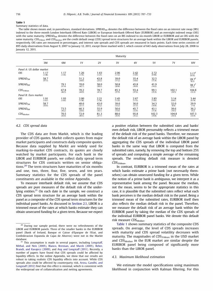
Table 1Summary statistics of data.

The table shows means and, in parentheses, standard deviations. SPREAD3M denotes the difference between the fixed rates on an interest rate swap (IRS)indexed to the three-month London Interbank Offered Rate (LIBOR) or European Interbank Offered Rate (EURIBOR) and an overnight indexed swap (OIS)with the same maturity. SPREAD6M denotes the difference between the fixed rates on an IRS indexed to six-month LIBOR or EURIBOR and an OIS with thesame maturity. CDSTrMean and CDSMedian are the credit default swap (CDS) spread term structures for an average bank within the LIBOR and EURIBOR panels,respectively. OIS rates are measured in percentages, and interest rate spreads and CDS spreads are measured in basis points. Each time series consists of895 daily observations from August 9, 2007 to January 12, 2011, except those marked with †, which consist of 643 daily observations from July 28, 2008 toJanuary 12, 2011.

Maturity

3M 6M 1Y 2Y 3Y 4Y 5Y 7Y 10Y

Panel A: US dollar marketOIS 1:17

ð1:48Þ1:17ð1:43Þ

1:26ð1:35Þ

1:63ð1:21Þ

2:06ð1:12Þ

2:42ð1:03Þ

2:72ð0:96Þ 3:17

ð0:55Þ†

SPREAD3M 58:7ð57:5Þ

51:2ð34:6Þ

43:8ð23:2Þ

39:0ð17:2Þ

35:4ð14:0Þ

32:5ð11:9Þ 28:7

ð8:2Þ†

SPREAD6M 79:1ð57:4Þ

70:0ð42:7Þ

58:0ð28:2Þ

50:8ð20:8Þ

45:8ð16:9Þ

41:9ð14:2Þ 38:1

ð7:7Þ†

CDSTrMean 67:8ð46:5Þ

70:2ð44:9Þ

78:7ð41:2Þ

85:3ð37:9Þ

93:4ð37:0Þ

99:1ð35:9Þ

102:1ð34:5Þ

104:8ð33:3Þ

Panel B: Euro marketOIS 1:91

ð1:67Þ1:93ð1:65Þ

2:00ð1:58Þ

2:21ð1:38Þ

2:45ð1:23Þ

2:67ð1:13Þ

2:85ð1:02Þ

3:14ð0:87Þ

3:44ð0:74Þ

SPREAD3M 58:7ð35:6Þ

49:6ð21:7Þ

43:0ð15:2Þ

39:6ð12:2Þ

36:0ð11:3Þ

34:3ð10:0Þ

32:0ð8:6Þ

29:9ð7:4Þ

SPREAD6M 73:5ð36:2Þ

66:3ð24:4Þ

55:9ð16:1Þ

50:6ð13:0Þ

45:7ð12:9Þ

43:1ð11:8Þ

39:6ð10:5Þ

36:2ð9:2Þ

CDSMedian 70:5ð43:0Þ

72:9ð40:5Þ

81:3ð37:7Þ

88:6ð35:9Þ

95:8ð35:2Þ

102:3ð34:8Þ

104:8ð34:4Þ

107:3ð33:9Þ

D. Filipović, A.B. Trolle / Journal of Financial Economics 109 (2013) 707–733716

4.2. CDS spread data

The CDS data are from Markit, which is the leadingprovider of CDS quotes. Markit collects quotes from majormarket participants and constructs daily composite quotes.Because data supplied by Markit are widely used formarking-to-market CDS contracts, its quotes are closelywatched by market participants. For each bank in theLIBOR and EURIBOR panels, we collect daily spread termstructures for CDS contracts written on senior obliga-tions.20 The term structures have maturities of six monthsand one, two, three, four, five, seven, and ten years.Summary statistics for the CDS spreads of the panelconstituents are available in the online Appendix.

To measure interbank default risk, we assume that CDSspreads are pure measures of the default risk of the under-lying entities.21 On each date in the sample, we construct aCDS spread term structure for an average bank within thepanel as a composite of the CDS spread term structures for theindividual panel banks. As discussed in Section 2.1, LIBOR is atrimmed mean of the rates at which banks estimate they canobtain unsecured funding for a given term. Because we expect

20 During our sample period, there were no refreshments of theLIBOR and EURIBOR panels. Three of the smaller banks in the EURIBORpanel (Bank of Ireland, Banque et Caisse d'Epargne de l'Etat, andConfederacion Espanola de Cajas de Ahorros) were not in the Markitdatabase.

21 This assumption is made in several papers, including Longstaff,Mithal, and Neis (2005), Blanco, Brennan, and Marsh (2005), Beber,Brandt, and Kavajecz (2009), and Ang and Longstaff (2011). Recently, anumber of papers have found that CDS spreads could be affected byliquidity effects. In the online Appendix, we show that our results arerobust to taking realistic CDS liquidity effects into account. While CDSspreads also could be affected by counterparty risk, Arora, Gandhi, andLongstaff (2012) find that this effect is minimal, which is consistent withthe widespread use of collateralization and netting agreements.

a positive relation between the submitted rates and banks'own default risk, LIBOR presumably reflects a trimmed meanof the default risk of the panel banks. Therefore, we measurethe default risk of an average bank within the LIBOR panel byaggregating the CDS spreads of the individual LIBOR panelbanks in the same way that LIBOR is computed from thesubmitted rates, namely, by removing the top and bottom 25%of spreads and computing a simple average of the remainingspreads. The resulting default risk measure is denotedCDSTrMean.

In contrast, EURIBOR is a trimmed mean of the rates atwhich banks estimate a prime bank (not necessarily them-selves) can obtain unsecured funding for a given term. Whilethe notion of a prime bank is ambiguous, we interpret it as arepresentative bank among the panel. Because the median,not the mean, seems to be the appropriate statistics in thiscase, it is plausible that the submitted rates reflect what eachbank perceives is the median default risk in the panel. Being atrimmed mean of the submitted rates, EURIBOR itself thenalso reflects the median default risk in the panel. Therefore,we measure the default risk of an average bank within theEURIBOR panel by taking the median of the CDS spreads ofthe individual EURIBOR panel banks. We denote this defaultrisk measure CDSMedian.

Table 1 shows summary statistics of the composite CDSspreads. On average, the level of CDS spreads increaseswith maturity and CDS spread volatility decreases withmaturity. The magnitudes of CDSTrMean in the USD marketand CDSMedian in the EUR market are similar despite theEURIBOR panel being composed of significantly morebanks than the LIBOR panel.

4.3. Maximum likelihood estimation

We estimate the model specifications using maximumlikelihood in conjunction with Kalman filtering. For this

D. Filipović, A.B. Trolle / Journal of Financial Economics 109 (2013) 707–733 717

purpose, we cast the model in state space form witha measurement equation describing the relationbetween the state variables and the observable interestrates and spreads, as well as a transition equationdescribing the discrete-time dynamics of the statevariables.22

Let Xt denote the vector of state variables and let Ztdenote the vector consisting of the term structure of OISrates, the two term structures of IRS-OIS spreads, and theterm structure of CDS spreads observed at time t. Themeasurement equation is given by

Zt ¼ h Xt ;Θð Þ þ ut ; ut∼N 0;Σð Þ; ð39Þ

where h is the pricing function, Θ is the vector of modelparameters, and ut is a vector of i.i.d. Gaussian pricingerrors with covariance matrix Σ. To reduce the number ofparameters in Σ, we follow usual practice in the empiricalterm structure literature in assuming that the pricingerrors are cross-sectionally uncorrelated (that is, Σ isdiagonal) and that the same variance, s2err , applies to allpricing errors. The observed instruments (OIS rates, IRS-OIS spreads, and CDS spreads) are linked to the statevariables as follows: OIS rates are related to the r(t)-process and Λ via Eqs. (11) and (3). CDS spreads are relatedto λ t0; tð Þ and, hence, the ν tð Þ-process and Λ via Eqs. (17)and (23)–(25). Finally, IRS-OIS spreads are related to λ t0; tð Þand Ξ t0; Tð Þ and, hence, the ν tð Þ- and ξ tð Þ-processes (theeffect of Λ more or less cancels) via Eqs. (12) and (22) inconjunction with Eqs. (3) and (18).23

While the transition density of Xt is unknown, itsconditional mean and variance is known in closed form,because Xt follows an affine diffusion process under theobjective probability measure. We approximate the transi-tion density with a Gaussian density with identical firstand second moments, in which case the transition equa-tion is of the form

Xt ¼Φ0 þ ΦXXt−1 þwt ; wt∼N 0;Qtð Þ; ð40Þ

where Qt is an affine function of Xt−1.Due to the nonlinearities in the relation between

observations and state variables, we apply the nonlinearunscented Kalman filter, which is found by Christoffersen,Jacobs, Karoui, and Mimouni (2009) to have very goodfinite-sample properties in the context of estimatingdynamic term structure models with swap rates. Detailsare provided in Appendix D. The Kalman filter producesone-step-ahead forecasts for Zt, Z tjt−1, and the correspond-

22 In the online Appendix, we consider an alternative two-stagemaximum likelihood procedure inspired by Duffee (1999) and Duffie,Pedersen, and Singleton (2003), which breaks the large estimationproblem into two smaller and more manageable estimation problems.The two estimation approaches give very similar results, and we, there-fore, report results based on the single-stage maximum likelihoodprocedure outlined here.

23 CDS and IRS-OIS spreads also depend on the r(t)-process andΛ due to the discounting by rc(t), but this provides only weakidentification.

ing error covariance matrices, Ftjt−1, from which we con-struct the log-likelihood function

L Θð Þ ¼−12

∑T

t ¼ 1nt log 2π þ log Ftjt−1 þ Zt−Z tjt−1

⊤F−1tjt−1 Zt−Z tjt−1

���� �;

�����ð41Þ

where T¼895 is the number of observation dates and nt isthe (time-varying) number of observations in Zt. Themaximum likelihood estimator, Θ, is then

Θ ¼ arg maxΘ

L Θð Þ: ð42Þ

Approximating the true transition density with a Gaussianmakes this a quasi-maximum likelihood (QML) procedure.While QML estimation has been shown to be consistent inmany settings, it is in fact not consistent in a Kalman filtersetting, because the conditional covariance matrix Qt inthe recursions depends on the Kalman filter estimates ofthe state variables instead of the true, but unobservable,values; see, e.g., Duan and Simonato (1999). However,simulation results in several papers have shown this issueto be negligible in practice.

In terms of identification, we face several issues. First,we show in the online Appendix that it is very difficult toseparately identify ζλ (with 1=ζλ being the mean jump sizein the default intensity) and the process for ν tð Þ (theintensity of credit quality deterioration). Instead, it is themean rate of credit quality deterioration of an averagepanel bank, 1=ζλ

� �ν tð Þ, that matters for valuation. In the

estimation, we fix ζλ at 10, but the implied process for themean rate of credit quality deterioration is invariant to thechoice of ζλ.

Second, in a preliminary analysis, we find that it isdifficult to reliably estimate the default intensity of theperiodically refreshed panel, Λ. Its value is not identifiedfrom the OIS term structure and, in the absence of veryshort-term CDS spreads, is also hard to pin down from theCDS term structure.24 From Eqs. (4) and (21), we have thatΛ is the difference between the instantaneous proxy of theovernight unsecured interbank rate, L t; tð Þ, and the trulyrisk-free rate, r(t). Therefore, one can get an idea about themagnitude of Λ by examining the spreads between short-term OIS rates and repo rates, which are virtually risk-freedue to the practice of overcollateralization of repo loans;see, e.g., Longstaff (2000). The sample averages of thespreads between one-week OIS rates and one-week generalcollateral (GC) repo rates for Treasuries, agency securities,agency-issued mortgage-backed securities (MBSs), and Eur-opean government bonds are 13 bps, 3 bps, −1 bp, and 0 bp,

24 The OIS term structure depends on the model for the collateralrate, rc tð Þ ¼ r tð Þ þ Λ, under the risk-neutral measure, with r(t) given by Eq.(26). An equivalent model in which rc(t) is a state variable is

drc tð Þ ¼ κr ~γ tð Þ−rc tð Þð Þ dt þ sr dWr tð Þd~γ tð Þ ¼ κγ ~θγ−~γ tð Þ� �

dt þ sγ ρ dWr tð Þ þffiffiffiffiffiffiffiffiffiffiffi1−ρ2

pdWγ tð Þ

;

where ~γ tð Þ ¼ γ tð Þ þ Λ and ~θγ ¼ θγ þ Λ. The latter specification is maximallyflexible with six identifiable parameters, see Dai and Singleton (2000).Therefore, θγ and Λ are not separately identified from the OIS term structure.

D. Filipović, A.B. Trolle / Journal of Financial Economics 109 (2013) 707–733718

respectively.25 Plots of these spreads can be found in theonline Appendix. In the case of Treasury collateral, the spreadspikes at the beginning of the crisis and around the BearStearns and Lehman Brothers episodes. However, movementsin the spread likely reflect periodic scarcity of Treasurycollateral, rather than variation in default risk, because thespikes are mostly due to downward spikes in the Treasuryrepo rate, not upward spikes in the OIS rate. Also, thecorrelation between the OIS-Treasury repo spread and theshort-maturity (six-month) LIBOR panel CDS spread is vir-tually zero.26 In the cases of agency securities and agency-issued MBSs, the spreads are volatile in the first half of thesample period, but without systematic patterns around crisisevents. In the case of the EURmarket, the spread is very stablethroughout the sample period. Taken together, these resultssuggest that very little default risk exists in the market forovernight interbank deposits. We fix Λ at 5 bps, but reason-able variations in the value of Λ do not change our results. Inthe online Appendix, we show that our results are robust toextending the model with a stochastic Λ tð Þ identified via OIS-Treasury repo spreads.

Third, given the relatively short sample period, many ofthe market price of risk parameters are imprecisely esti-mated (in contrast to the risk-neutral parameters, most ofwhich are strongly identified with low standard errors).For each model specification, we obtain a more parsimo-nious risk premium structure by reestimating themodel after setting to zero those market price of riskparameters for which the absolute t-statistics did notexceed one.27 The likelihood functions were virtuallyunaffected by this, so we henceforth study these con-strained model specifications.

5. Results

We discuss estimates of parameters and state variables,compare model specifications, decompose the term structureof interbank risk, and quantify risk premiums.

25 Similar results are obtained by examining the spreads between FFand overnight GC repo rates for Treasuries, agency securities, and agency-issued MBSs as well as the spread between EONIA and the overnightEuropean GC repo rate. The sample averages of these spreads are 15 bps,5 bps, 2 bps, and 1 bp, respectively. Since overnight rates are highlyvolatile with predictable liquidity-driven jumps (see, e.g., Bartolini,Hilton, Sundaresan, and Tonetti, 2011), we believe the one-week OIS-repo spreads are more informative. As the European GC repo rate, we usethe Eurepo rate, which is a benchmark reflecting the rate on interbankborrowing secured by “the best collateral within the most actively tradedEuropean repo market,” see http://www.euribor-ebf.eu/eurepo-org/about-eurepo.html.

26 In their analysis of the repo market, Hordahl and King (2008, p.46) also note scarcity of Treasury collateral as the main factor drivingrepo spreads: “As the available supply of Treasury collateral dropped,those market participants willing to lend out Treasuries were able toborrow cash at increasingly cheap rates. At times, this effect pushed USGC repo rates down to levels only a few basis points above zero.”

27 A similar approach is taken by Duffee (2002) and Dai andSingleton (2002), among others. Alternative approaches to restrictingrisk premiums include using various information criteria to select theoptimal specification as in Joslin, Priebsch, and Singleton (2010) andadopting a Bayesian framework as in Bauer (2011).

5.1. Maximum likelihood estimates

Table 2 displays parameter estimates and their asymp-totic standard errors. It is straightforward to verify that, forall the specifications, the parameter values satisfy thesufficient admissability conditions in Lemma C.4 inAppendix C. The estimates are strikingly similar acrossthe two markets and, therefore, we focus on the USDestimates.

In the A 2;2;1ð Þ and A 2;2;2ð Þ specifications, ν tð Þ isrelatively volatile and displays fast mean-reversion towardμ tð Þ, which in turn is less volatile and has much slowermean-reversion. Hence, ν tð Þ captures transitory shocks tothe intensity of credit quality deterioration, while μ tð Þcaptures more persistent shocks. In the A 2;1;1ð Þ specifica-tion, the speed of mean-reversion and the volatility of ν tð Þlie between those of ν tð Þ and μ tð Þ in the more generalspecifications. Also, between jumps, the reversion of thedefault intensity toward Λ occurs relatively fast. Althoughestimated with some uncertainty, the market price of riskparameters Γν and Γμ are negative in all specifications. Thisimplies that the expected rate of credit quality deteriora-tion is lower under the physical measure than under therisk-neutral measure, indicating that market participantsrequire a premium for bearing exposure to variation indefault risk. This is consistent with several papers findingthat variation in default risk carries a risk premium; see, e.g., Duffee (1999) in the case of corporate default risk andPan and Singleton (2008) in the case of sovereign defaultrisk. We return to this issue in Section 5.6.

In all specifications, the residual factor, ξ tð Þ, is veryvolatile, exhibits very fast mean-reversion, and has a long-run mean of essentially zero. In the A 2;2;2ð Þ specifica-tions, ξ tð Þ is mean-reverting toward ϵ tð Þ, which is lessvolatile and has slower mean-reversion. Hence, ξ tð Þ cap-tures transitory shocks to the non-default component andϵ tð Þ captures moderately persistent shocks. In none of thespecifications were we able to reliably estimate Γξ and Γϵ.Consequently, these parameters were constrained to zero(see end of Section 4.3).

5.2. State variables

Fig. 2 displays the state variables for the three specifi-cations estimated on USD data. The corresponding figurefor the EUR market is similar and available in the onlineAppendix. It is instructive to see the reaction of the statevariables to the three most important shocks to theinterbank money market during the sample period: theBear Stearns near-bankruptcy on March 16, 2008, theLehman Brothers bankruptcy on September 15, 2008,and the escalation of the European sovereign debt crisisoften marked by the downgrade of Greece's debt to non-investment-grade status by Standard and Poor's on April27, 2010. The figure shows that ν tð Þ increases leading up tothe Bear Stearns near-default but quickly decreases afterthe takeover by J.P. Morgan. If anything, the opposite istrue of ξ tð Þ. Immediately following the Lehman default, ξ tð Þspikes while ν tð Þ increases more gradually and does notreach its maximum until March 2009. Finally, with theescalation of the European sovereign debt crisis, ν tð Þ

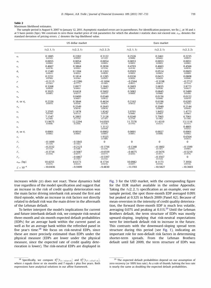
Table 2Maximum likelihood estimates.

The sample period is August 9, 2007 to January 12, 2011. Asymptotic standard errors are in parentheses. For identification purposes, we fix ζλ at 10 and Λ

at 5 basis points (bps). We constrain to zero those market price of risk parameters for which the absolute t-statistic does not exceed one. serr denotes thestandard deviation of pricing errors. L denotes the log-likelihood value.

US dollar market Euro market

Að2;1;1Þ Að2;2;1Þ Að2;2;2Þ Að2;1;1Þ Að2;2;1Þ Að2;2;2Þ

κr 0:1885ð0:0143Þ

0:2282ð0:0205Þ

0:3122ð0:1322Þ

0:2526ð0:0068Þ

0:2461ð0:0042Þ

0:2235ð0:0031Þ

sr 0:0055ð0:0004Þ

0:0054ð0:0003Þ

0:0054ð0:0003Þ

0:0053ð0:0003Þ

0:0053ð0:0003Þ

0:0051ð0:0002Þ

κγ 0:4667ð0:0278Þ

0:3864ð0:0303Þ

0:2836ð0:1234Þ

0:4703ð0:0156Þ

0:4663ð0:0097Þ

0:4566ð0:0076Þ

θγ 0:1340ð0:0031Þ

0:1304ð0:0022Þ

0:1263ð0:0020Þ

0:0503ð0:0003Þ

0:0514ð0:0003Þ

0:0603ð0:0009Þ

sγ 0:2251ð0:0180Þ

0:1814ð0:0166Þ

0:1285ð0:0547Þ

0:0336ð0:0026Þ

0:0415ð0:0029Þ

0:0808ð0:0044Þ

ρ −0:2115ð0:2365Þ

−0:2286ð0:1771Þ

−0:1694ð0:1965Þ

−0:2564ð0:0831Þ

−0:3198ð0:0813Þ

−0:2712ð0:1319Þ

κν 0:3268ð0:0020Þ

2:0977ð0:0493Þ

2:1843ð0:0697Þ

0:2603ð0:0019Þ

2:6835ð0:0528Þ

2:8773ð0:0627Þ

sν 0:3925ð0:0085Þ

0:6418ð0:0577Þ

0:5602ð0:0537Þ

0:3082ð0:0069Þ

0:6845ð0:0488Þ

0:5489ð0:0396Þ

κμ 0:0499ð0:0067Þ

0:0340ð0:0072Þ

0:0156ð0:0046Þ

0:0152ð0:0079Þ

θν or θμ 0:2326ð0:0019Þ

0:3844ð0:0258Þ

0:4634ð0:0635Þ

0:2162ð0:0012Þ

0:6196ð0:1268Þ

0:6285ð0:2555Þ

sμ 0:2549ð0:0074Þ

0:2643ð0:0074Þ

0:2049ð0:0047Þ

0:2144ð0:0056Þ

κλ 2:2595ð0:0149Þ

2:1878ð0:0113Þ

1:8242ð0:0159Þ

2:0701ð0:0086Þ

1:8452ð0:0083Þ

1:4773ð0:0083Þ

κξ 7:1547ð0:2180Þ

6:2883ð0:1114Þ

7:2128ð0:1187Þ

6:0240ð0:2739Þ

5:7965ð0:1982Þ

6:7061ð0:1504Þ

sξ 13:9675ð0:4648Þ

12:2294ð0:2364Þ

14:0501ð0:2538Þ

11:7578ð0:5793Þ

11:4319ð0:4121Þ

13:1116ð0:3151Þ

κϵ 1:3112ð0:0594Þ

0:4801ð0:0252Þ

θξ or θϵ 0:0001ð0:0002Þ

0:0010ð0:0005Þ

0:0002ð0:0001Þ

0:0001ð0:0001Þ

0:0027ð0:0008Þ

0:0001ð0:0002Þ

sϵ 1:9325ð0:1089Þ

0:6564ð0:0415Þ

Γr −0:1499ð0:1324Þ

−0:1843ð0:1562Þ

0 0 0 0

Γγ −0:2332ð0:1154Þ

−0:2123ð0:1298Þ

−0:1756ð0:1256Þ

−0:1348ð0:0781Þ

−0:1802ð0:1187Þ

−0:1599ð0:0985Þ

Γν −0:3734ð0:3354Þ

−0:5687ð0:4377Þ

−0:6559ð0:4177Þ

−0:4675ð0:4243Þ

−0:5476ð0:3911Þ

−0:5210ð0:3576Þ

Γμ −0:4467ð0:1765Þ

−0:5397ð0:2332Þ

−0:3567ð0:3124Þ

0

serr (bp) 10:4255ð0:0235Þ

8:6173ð0:0223Þ

8:1734ð0:0216Þ

10:0982ð0:0207Þ

8:1173ð0:0166Þ

7:3956ð0:0154Þ

L� 10−4 −10.0436 −9.5909 −9.4830 −11.1765 −10.5827 −10.3603

D. Filipović, A.B. Trolle / Journal of Financial Economics 109 (2013) 707–733 719

increases while ξ tð Þ does not react. These dynamics holdtrue regardless of the model specification and suggest thatan increase in the risk of credit quality deterioration wasthe main factor driving interbank risk around the first andthird episode, while an increase in risk factors not directlyrelated to default risk was the main driver in the aftermathof the Lehman default.

To better interpret the model's implications for currentand future interbank default risk, we compute risk-neutralthree-month and six-month expected default probabilities(EDPs) for an average bank within the current panel aswell as for an average bank within the refreshed panel infive year's time.28 We focus on risk-neutral EDPs, sincethese are more precisely estimated than EDPs under thephysical measure (EDPs are lower under the physicalmeasure, since the expected rate of credit quality dete-rioration is lower). The risk-neutral EDPs are displayed in

28 Specifically, we compute EQt 1fto τ tð Þ≤tþδg�

and EQt 1fTo τ Tð Þ≤Tþδg�

,where δ equals three or six months and T equals t plus five years. Bothexpressions have analytical solutions in our affine framework.

Fig. 3 for the USD market, with the corresponding figurefor the EUR market available in the online Appendix.Taking the A 2;2;1ð Þ specification as an example, over oursample period, the spot three-month EDP averaged 0.09%but peaked at 0.32% in March 2009 (Panel A2). Because ofmean-reversion in the intensity of credit quality deteriora-tion, the forward three-month EDP is much less volatile,averaging 0.07% and peaking at 0.11%.29 Until the LehmanBrothers default, the term structure of EDPs was mostlyupward-sloping, implying that risk-neutral expectationswere for interbank default risk to increase in the future.This contrasts with the downward-sloping spread termstructure during this period (see Fig. 1), indicating animportant role for non-default risk factors in determiningshorter-term spreads. From the Lehman Brothersdefault until fall 2009, the term structure of EDPs was

29 The expected default probabilities depend on our assumption ofzero recovery (or 100% loss rate). As a rule of thumb, halving the loss rateis nearly the same as doubling the expected default probabilities.

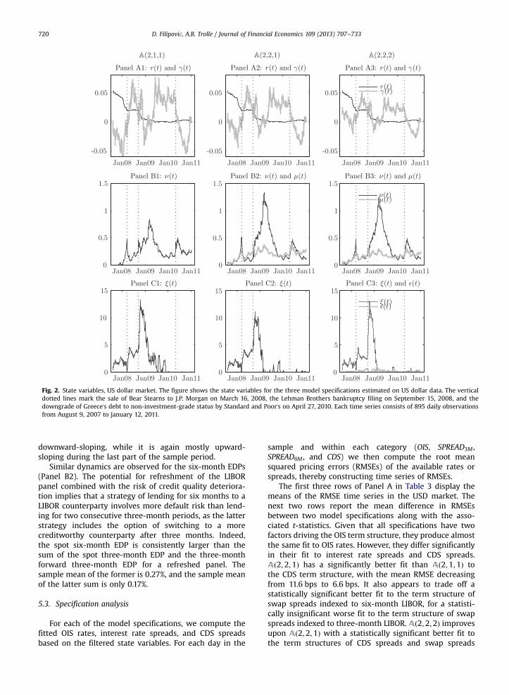
Fig. 2. State variables, US dollar market. The figure shows the state variables for the three model specifications estimated on US dollar data. The verticaldotted lines mark the sale of Bear Stearns to J.P. Morgan on March 16, 2008, the Lehman Brothers bankruptcy filing on September 15, 2008, and thedowngrade of Greece's debt to non-investment-grade status by Standard and Poor's on April 27, 2010. Each time series consists of 895 daily observationsfrom August 9, 2007 to January 12, 2011.

D. Filipović, A.B. Trolle / Journal of Financial Economics 109 (2013) 707–733720

downward-sloping, while it is again mostly upward-sloping during the last part of the sample period.

Similar dynamics are observed for the six-month EDPs(Panel B2). The potential for refreshment of the LIBORpanel combined with the risk of credit quality deteriora-tion implies that a strategy of lending for six months to aLIBOR counterparty involves more default risk than lend-ing for two consecutive three-month periods, as the latterstrategy includes the option of switching to a morecreditworthy counterparty after three months. Indeed,the spot six-month EDP is consistently larger than thesum of the spot three-month EDP and the three-monthforward three-month EDP for a refreshed panel. Thesample mean of the former is 0.27%, and the sample meanof the latter sum is only 0.17%.

5.3. Specification analysis

For each of the model specifications, we compute thefitted OIS rates, interest rate spreads, and CDS spreadsbased on the filtered state variables. For each day in the

sample and within each category (OIS, SPREAD3M ,SPREAD6M , and CDS) we then compute the root meansquared pricing errors (RMSEs) of the available rates orspreads, thereby constructing time series of RMSEs.

The first three rows of Panel A in Table 3 display themeans of the RMSE time series in the USD market. Thenext two rows report the mean difference in RMSEsbetween two model specifications along with the asso-ciated t-statistics. Given that all specifications have twofactors driving the OIS term structure, they produce almostthe same fit to OIS rates. However, they differ significantlyin their fit to interest rate spreads and CDS spreads.A 2;2;1ð Þ has a significantly better fit than A 2;1;1ð Þ tothe CDS term structure, with the mean RMSE decreasingfrom 11.6 bps to 6.6 bps. It also appears to trade off astatistically significant better fit to the term structure ofswap spreads indexed to six-month LIBOR, for a statisti-cally insignificant worse fit to the term structure of swapspreads indexed to three-month LIBOR. A 2;2;2ð Þ improvesupon A 2;2;1ð Þ with a statistically significant better fit tothe term structures of CDS spreads and swap spreads

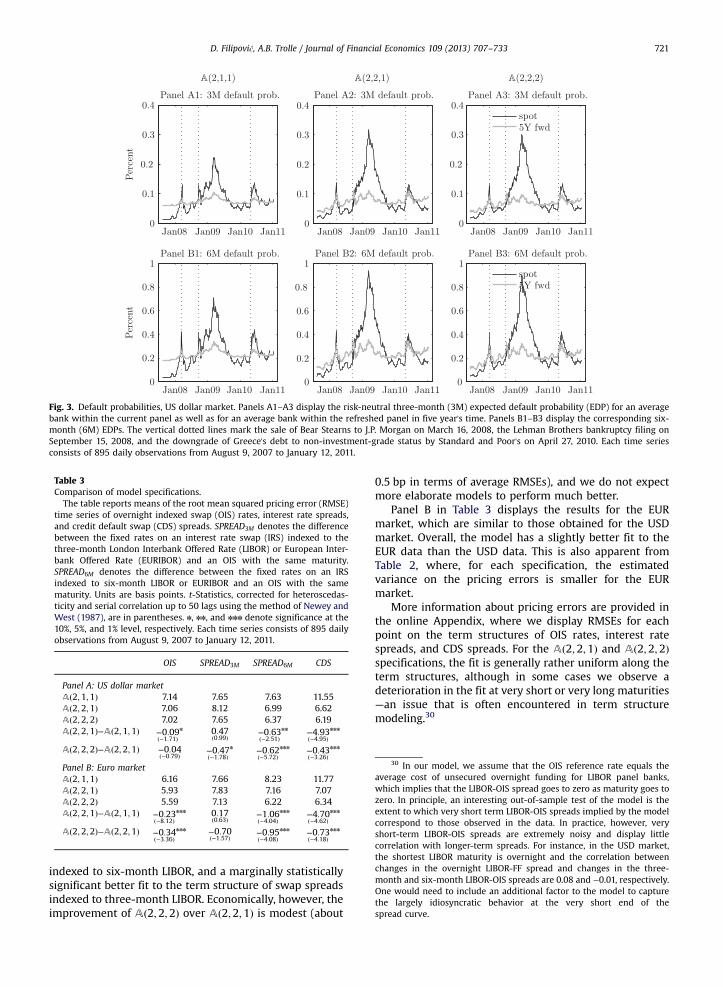
Fig. 3. Default probabilities, US dollar market. Panels A1–A3 display the risk-neutral three-month (3M) expected default probability (EDP) for an averagebank within the current panel as well as for an average bank within the refreshed panel in five year's time. Panels B1–B3 display the corresponding six-month (6M) EDPs. The vertical dotted lines mark the sale of Bear Stearns to J.P. Morgan on March 16, 2008, the Lehman Brothers bankruptcy filing onSeptember 15, 2008, and the downgrade of Greece's debt to non-investment-grade status by Standard and Poor's on April 27, 2010. Each time seriesconsists of 895 daily observations from August 9, 2007 to January 12, 2011.

Table 3Comparison of model specifications.

The table reports means of the root mean squared pricing error (RMSE)time series of overnight indexed swap (OIS) rates, interest rate spreads,and credit default swap (CDS) spreads. SPREAD3M denotes the differencebetween the fixed rates on an interest rate swap (IRS) indexed to thethree-month London Interbank Offered Rate (LIBOR) or European Inter-bank Offered Rate (EURIBOR) and an OIS with the same maturity.SPREAD6M denotes the difference between the fixed rates on an IRSindexed to six-month LIBOR or EURIBOR and an OIS with the samematurity. Units are basis points. t-Statistics, corrected for heteroscedas-ticity and serial correlation up to 50 lags using the method of Newey andWest (1987), are in parentheses. n, nn, and nnn denote significance at the10%, 5%, and 1% level, respectively. Each time series consists of 895 dailyobservations from August 9, 2007 to January 12, 2011.

OIS SPREAD3M SPREAD6M CDS

Panel A: US dollar marketAð2;1;1Þ 7.14 7.65 7.63 11.55Að2;2;1Þ 7.06 8.12 6.99 6.62Að2;2;2Þ 7.02 7.65 6.37 6.19Að2;2;1Þ−Að2;1;1Þ −0:09

ð−1:71Þn 0:47

ð0:99Þ −0:63ð−2:51Þ

nn −4:93ð−4:95Þ

nnn

Að2;2;2Þ−Að2;2;1Þ −0:04ð−0:79Þ −0:47

ð−1:78Þn −0:62

ð−5:72Þnnn −0:43

ð−3:26Þnnn

Panel B: Euro marketAð2;1;1Þ 6.16 7.66 8.23 11.77Að2;2;1Þ 5.93 7.83 7.16 7.07Að2;2;2Þ 5.59 7.13 6.22 6.34Að2;2;1Þ−Að2;1;1Þ −0:23

ð−8:12Þnnn 0:17

ð0:63Þ −1:06ð−4:04Þ

nnn −4:70ð−4:62Þ

nnn

Að2;2;2Þ−Að2;2;1Þ −0:34ð−3:36Þ

nnn −0:70ð−1:57Þ −0:95

ð−4:08Þnnn −0:73

ð−4:18Þnnn

30 In our model, we assume that the OIS reference rate equals theaverage cost of unsecured overnight funding for LIBOR panel banks,which implies that the LIBOR-OIS spread goes to zero as maturity goes tozero. In principle, an interesting out-of-sample test of the model is theextent to which very short term LIBOR-OIS spreads implied by the modelcorrespond to those observed in the data. In practice, however, veryshort-term LIBOR-OIS spreads are extremely noisy and display littlecorrelation with longer-term spreads. For instance, in the USD market,the shortest LIBOR maturity is overnight and the correlation betweenchanges in the overnight LIBOR-FF spread and changes in the three-month and six-month LIBOR-OIS spreads are 0.08 and −0.01, respectively.One would need to include an additional factor to the model to capturethe largely idiosyncratic behavior at the very short end of thespread curve.

D. Filipović, A.B. Trolle / Journal of Financial Economics 109 (2013) 707–733 721

indexed to six-month LIBOR, and a marginally statisticallysignificant better fit to the term structure of swap spreadsindexed to three-month LIBOR. Economically, however, theimprovement of A 2;2;2ð Þ over A 2;2;1ð Þ is modest (about

0.5 bp in terms of average RMSEs), and we do not expectmore elaborate models to perform much better.

Panel B in Table 3 displays the results for the EURmarket, which are similar to those obtained for the USDmarket. Overall, the model has a slightly better fit to theEUR data than the USD data. This is also apparent fromTable 2, where, for each specification, the estimatedvariance on the pricing errors is smaller for the EURmarket.

More information about pricing errors are provided inthe online Appendix, where we display RMSEs for eachpoint on the term structures of OIS rates, interest ratespreads, and CDS spreads. For the A 2;2;1ð Þ and A 2;2;2ð Þspecifications, the fit is generally rather uniform along theterm structures, although in some cases we observe adeterioration in the fit at very short or very long maturities—an issue that is often encountered in term structuremodeling.30

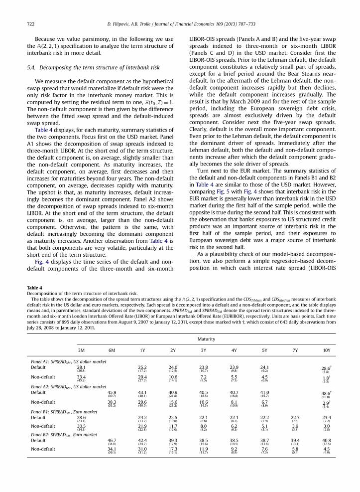
D. Filipović, A.B. Trolle / Journal of Financial Economics 109 (2013) 707–733722

Because we value parsimony, in the following we usethe A 2;2;1ð Þ specification to analyze the term structure ofinterbank risk in more detail.

5.4. Decomposing the term structure of interbank risk

We measure the default component as the hypotheticalswap spread that would materialize if default risk were theonly risk factor in the interbank money market. This iscomputed by setting the residual term to one, Ξ t0; Tð Þ ¼ 1.The non-default component is then given by the differencebetween the fitted swap spread and the default-inducedswap spread.

Table 4 displays, for each maturity, summary statistics ofthe two components. Focus first on the USD market. PanelA1 shows the decomposition of swap spreads indexed tothree-month LIBOR. At the short end of the term structure,the default component is, on average, slightly smaller thanthe non-default component. As maturity increases, thedefault component, on average, first decreases and thenincreases for maturities beyond four years. The non-defaultcomponent, on average, decreases rapidly with maturity.The upshot is that, as maturity increases, default increas-ingly becomes the dominant component. Panel A2 showsthe decomposition of swap spreads indexed to six-monthLIBOR. At the short end of the term structure, the defaultcomponent is, on average, larger than the non-defaultcomponent. Otherwise, the pattern is the same, withdefault increasingly becoming the dominant componentas maturity increases. Another observation from Table 4 isthat both components are very volatile, particularly at theshort end of the term structure.

Fig. 4 displays the time series of the default and non-default components of the three-month and six-month

Table 4Decomposition of the term structure of interbank risk.

The table shows the decomposition of the spread term structures using the Að2default risk in the US dollar and euro markets, respectively. Each spread is decommeans and, in parentheses, standard deviations of the two components. SPREADmonth and six-month London Interbank Offered Rate (LIBOR) or European Interbseries consists of 895 daily observations from August 9, 2007 to January 12, 2011,July 28, 2008 to January 12, 2011.

3M 6M 1Y 2Y

Panel A1: SPREAD3M , US dollar marketDefault 28:1

ð26:8Þ25:2ð17:2Þ

24:0ð12:5Þ

Non-default 33:4ð45:2Þ

20:4ð27:3Þ

10:6ð14:1Þ

Panel A2: SPREAD6M , US dollar marketDefault 45:9

ð39:7Þ43:1ð30:1Þ

40:9ð21:8Þ

Non-default 38:3ð53:2Þ

29:6ð40:5Þ

15:6ð21:2Þ

Panel B1: SPREAD3M , Euro marketDefault 28:6

ð23:1Þ24:2ð13:7Þ

22:5ð10:0Þ

Non-default 30:5ð34:1Þ

21:9ð22:8Þ

11:7ð12:0Þ

Panel B2: SPREAD6M, Euro marketDefault 46:7

ð34:0Þ42:4ð24:7Þ

39:3ð17:9Þ

Non-default 34:1ð36:1Þ

31:0ð31:2Þ

17:3ð17:1Þ

LIBOR-OIS spreads (Panels A and B) and the five-year swapspreads indexed to three-month or six-month LIBOR(Panels C and D) in the USD market. Consider first theLIBOR-OIS spreads. Prior to the Lehman default, the defaultcomponent constitutes a relatively small part of spreads,except for a brief period around the Bear Stearns near-default. In the aftermath of the Lehman default, the non-default component increases rapidly but then declines,while the default component increases gradually. Theresult is that by March 2009 and for the rest of the sampleperiod, including the European sovereign debt crisis,spreads are almost exclusively driven by the defaultcomponent. Consider next the five-year swap spreads.Clearly, default is the overall more important component.Even prior to the Lehman default, the default component isthe dominant driver of spreads. Immediately after theLehman default, both the default and non-default compo-nents increase after which the default component gradu-ally becomes the sole driver of spreads.

Turn next to the EUR market. The summary statistics ofthe default and non-default components in Panels B1 and B2in Table 4 are similar to those of the USD market. However,comparing Fig. 5 with Fig. 4 shows that interbank risk in theEUR market is generally lower than interbank risk in the USDmarket during the first half of the sample period, while theopposite is true during the second half. This is consistent withthe observation that banks' exposures to US structured creditproducts was an important source of interbank risk in thefirst half of the sample period, and their exposures toEuropean sovereign debt was a major source of interbankrisk in the second half.

As a plausibility check of our model-based decomposi-tion, we also perform a simple regression-based decom-position in which each interest rate spread (LIBOR-OIS

;2;1Þ specification and the CDSTrMean and CDSMedian measures of interbankposed into a default and a non-default component, and the table displays

3M and SPREAD6M denote the spread term structures indexed to the three-ank Offered Rate (EURIBOR), respectively. Units are basis points. Each timeexcept those marked with †, which consist of 643 daily observations from

Maturity

3Y 4Y 5Y 7Y 10Y

23:8ð10:7Þ

23:9ð9:8Þ

24:1ð9:2Þ 28:6

ð5:8Þ†

7:2ð9:5Þ

5:5ð7:3Þ

4:5ð6:0Þ 1:8

ð3:5Þ†

40:5ð18:5Þ

40:7ð16:8Þ

41:0ð15:7Þ 48:6

ð10:0Þ†

10:6ð14:3Þ

8:1ð10:9Þ

6:7ð8:9Þ 2:9

ð5:4Þ†

22:1ð8:8Þ

22:1ð8:2Þ

22:2ð7:9Þ

22:7ð7:5Þ

23:4ð7:2Þ

8:0ð8:2Þ

6:2ð6:3Þ

5:1ð5:1Þ

3:9ð3:8Þ

3:0ð2:8Þ

38:5ð15:6Þ

38:5ð14:5Þ

38:7ð13:8Þ

39:4ð13:1Þ

40:8ð12:5Þ

11:9ð11:7Þ

9:2ð8:9Þ

7:6ð7:3Þ

5:8ð5:4Þ

4:5ð4:0Þ

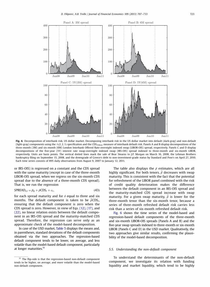
Fig. 4. Decomposition of interbank risk, US dollar market. Decomposing interbank risk in the US dollar market into default (dark-gray) and non-default(light-gray) components using the Að2;2;1Þ specification and the CDSTrMean measure of interbank default risk. Panels A and B display decompositions of thethree-month (3M) and six-month (6M) London Interbank Offered Rate-overnight indexed swap (LIBOR-OIS) spread, respectively. Panels C and D displaydecompositions of the five-year (5Y) interest rate swap-overnight indexed swap (IRS-OIS) spread indexed to three-month and six-month LIBOR,respectively. Units are basis points. The vertical dotted lines mark the sale of Bear Stearns to J.P. Morgan on March 16, 2008, the Lehman Brothersbankruptcy filing on September 15, 2008, and the downgrade of Greece's debt to non-investment-grade status by Standard and Poor's on April 27, 2010.Each time series consists of 895 daily observations from August 9, 2007 to January 12, 2011.

D. Filipović, A.B. Trolle / Journal of Financial Economics 109 (2013) 707–733 723

or IRS-OIS) is regressed on a constant and the CDS spreadwith the same maturity (except in case of the three-monthLIBOR-OIS spread, when we regress on the six-month CDSspread due to the absence of a three-month CDS spread).That is, we run the regression

SPREADδ;t ¼ β0 þ βCDSt þ ϵt ; ð43Þfor each spread maturity and for δ equal to three and sixmonths. The default component is taken to be bβCDSt ,ensuring that the default component is zero when theCDS spread is zero. However, in view of Eqs. (12), (17), and(22), no linear relation exists between the default compo-nent in an IRS-OIS spread and the maturity-matched CDSspread. Therefore, the regression can serve only as anapproximate check of the model-based decomposition.

In case of the USD market, Table 5 displays the means and,in parentheses, standard deviations of the default componentsobtained via the two approaches. The regression-baseddefault component tends to be lower, on average, and lessvolatile than the model-based default component, particularlyat longer maturities.31

31 The flip-side is that the regression-based non-default componenttends to be higher, on average, and more volatile than the model-basednon-default component.

The table also displays the β estimates, which are allhighly significant. For both tenors, bβ decreases with swapmaturity. This is consistent with the fact that the potentialfor refreshment of the LIBOR panel combined with the riskof credit quality deterioration makes the differencebetween the default component in an IRS-OIS spread andthe maturity-matched CDS spread increase with swapmaturity. For a given swap maturity, bβ is lower for thethree-month tenor than the six-month tenor, because aseries of three-month refreshed default risk carries lessrisk than a series of six-month refreshed default risk.

Fig. 6 shows the time series of the model-based andregression-based default components of the three-monthand six-month LIBOR-OIS spreads (Panels A and B) and thefive-year swap spreads indexed to three-month or six-monthLIBOR (Panels C and D) in the USD market. Qualitatively, thetwo approaches give similar results, confirming the plausi-bility of the model-based decomposition.

5.5. Understanding the non-default component

To understand the determinants of the non-defaultcomponent, we investigate its relation with fundingliquidity and market liquidity, which tend to be highly

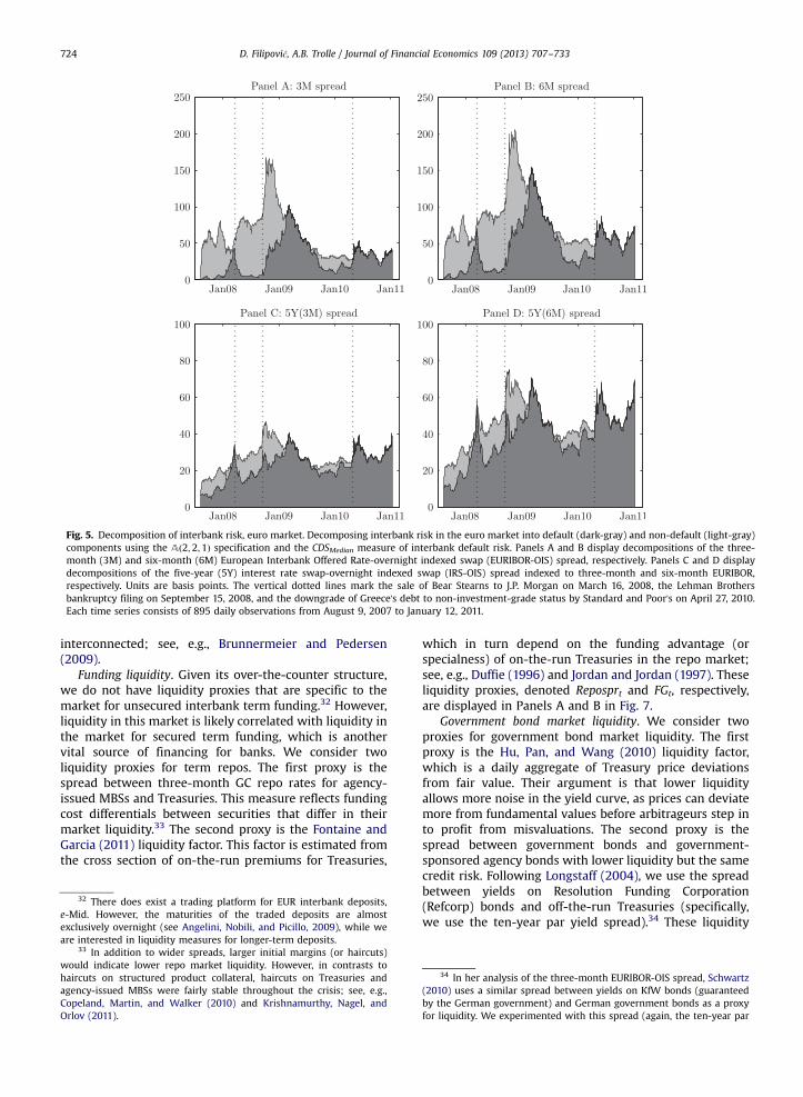
Fig. 5. Decomposition of interbank risk, euro market. Decomposing interbank risk in the euro market into default (dark-gray) and non-default (light-gray)components using the Að2;2;1Þ specification and the CDSMedian measure of interbank default risk. Panels A and B display decompositions of the three-month (3M) and six-month (6M) European Interbank Offered Rate-overnight indexed swap (EURIBOR-OIS) spread, respectively. Panels C and D displaydecompositions of the five-year (5Y) interest rate swap-overnight indexed swap (IRS-OIS) spread indexed to three-month and six-month EURIBOR,respectively. Units are basis points. The vertical dotted lines mark the sale of Bear Stearns to J.P. Morgan on March 16, 2008, the Lehman Brothersbankruptcy filing on September 15, 2008, and the downgrade of Greece's debt to non-investment-grade status by Standard and Poor's on April 27, 2010.Each time series consists of 895 daily observations from August 9, 2007 to January 12, 2011.

D. Filipović, A.B. Trolle / Journal of Financial Economics 109 (2013) 707–733724

interconnected; see, e.g., Brunnermeier and Pedersen(2009).

Funding liquidity. Given its over-the-counter structure,we do not have liquidity proxies that are specific to themarket for unsecured interbank term funding.32 However,liquidity in this market is likely correlated with liquidity inthe market for secured term funding, which is anothervital source of financing for banks. We consider twoliquidity proxies for term repos. The first proxy is thespread between three-month GC repo rates for agency-issued MBSs and Treasuries. This measure reflects fundingcost differentials between securities that differ in theirmarket liquidity.33 The second proxy is the Fontaine andGarcia (2011) liquidity factor. This factor is estimated fromthe cross section of on-the-run premiums for Treasuries,

32 There does exist a trading platform for EUR interbank deposits,e-Mid. However, the maturities of the traded deposits are almostexclusively overnight (see Angelini, Nobili, and Picillo, 2009), while weare interested in liquidity measures for longer-term deposits.

33 In addition to wider spreads, larger initial margins (or haircuts)would indicate lower repo market liquidity. However, in contrasts tohaircuts on structured product collateral, haircuts on Treasuries andagency-issued MBSs were fairly stable throughout the crisis; see, e.g.,Copeland, Martin, and Walker (2010) and Krishnamurthy, Nagel, andOrlov (2011).

which in turn depend on the funding advantage (orspecialness) of on-the-run Treasuries in the repo market;see, e.g., Duffie (1996) and Jordan and Jordan (1997). Theseliquidity proxies, denoted Reposprt and FGt, respectively,are displayed in Panels A and B in Fig. 7.

Government bond market liquidity. We consider twoproxies for government bond market liquidity. The firstproxy is the Hu, Pan, and Wang (2010) liquidity factor,which is a daily aggregate of Treasury price deviationsfrom fair value. Their argument is that lower liquidityallows more noise in the yield curve, as prices can deviatemore from fundamental values before arbitrageurs step into profit from misvaluations. The second proxy is thespread between government bonds and government-sponsored agency bonds with lower liquidity but the samecredit risk. Following Longstaff (2004), we use the spreadbetween yields on Resolution Funding Corporation(Refcorp) bonds and off-the-run Treasuries (specifically,we use the ten-year par yield spread).34 These liquidity

34 In her analysis of the three-month EURIBOR-OIS spread, Schwartz(2010) uses a similar spread between yields on KfW bonds (guaranteedby the German government) and German government bonds as a proxyfor liquidity. We experimented with this spread (again, the ten-year par

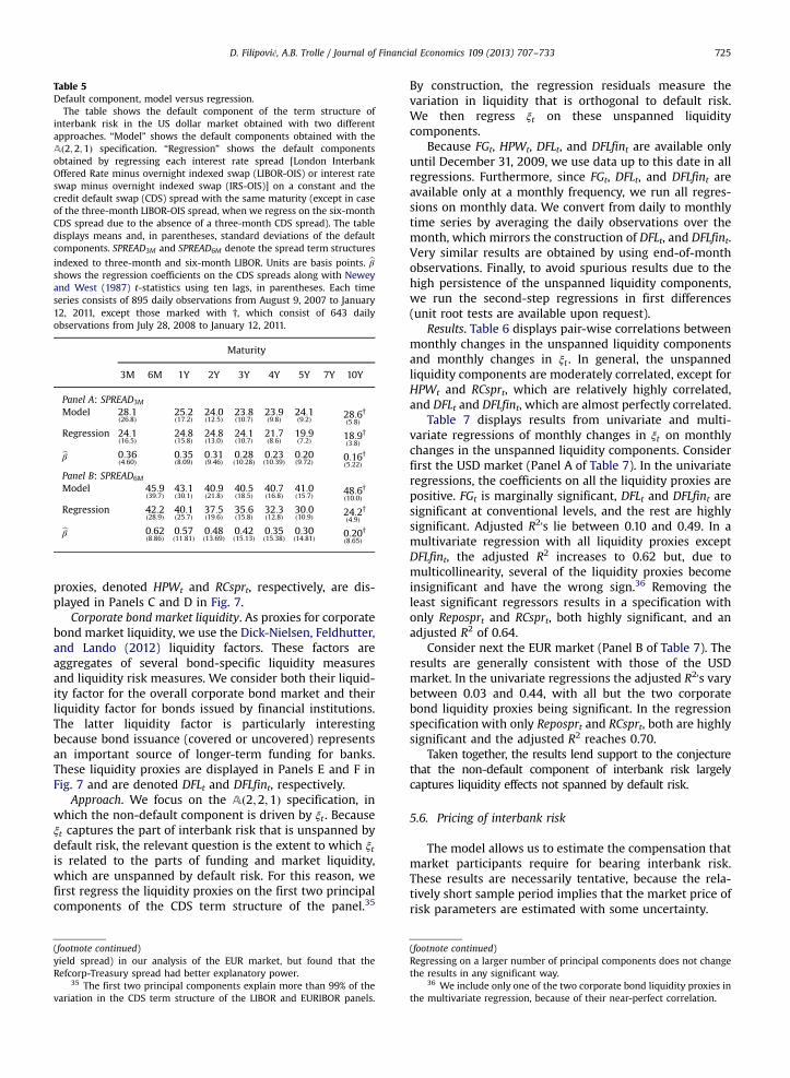
Table 5Default component, model versus regression.

The table shows the default component of the term structure ofinterbank risk in the US dollar market obtained with two differentapproaches. “Model” shows the default components obtained with theAð2;2;1Þ specification. “Regression” shows the default componentsobtained by regressing each interest rate spread [London InterbankOffered Rate minus overnight indexed swap (LIBOR-OIS) or interest rateswap minus overnight indexed swap (IRS-OIS)] on a constant and thecredit default swap (CDS) spread with the same maturity (except in caseof the three-month LIBOR-OIS spread, when we regress on the six-monthCDS spread due to the absence of a three-month CDS spread). The tabledisplays means and, in parentheses, standard deviations of the defaultcomponents. SPREAD3M and SPREAD6M denote the spread term structures

indexed to three-month and six-month LIBOR. Units are basis points. bβshows the regression coefficients on the CDS spreads along with Neweyand West (1987) t-statistics using ten lags, in parentheses. Each timeseries consists of 895 daily observations from August 9, 2007 to January12, 2011, except those marked with †, which consist of 643 dailyobservations from July 28, 2008 to January 12, 2011.

Maturity

3M 6M 1Y 2Y 3Y 4Y 5Y 7Y 10Y

Panel A: SPREAD3M

Model 28:1ð26:8Þ

25:2ð17:2Þ

24:0ð12:5Þ

23:8ð10:7Þ

23:9ð9:8Þ

24:1ð9:2Þ 28:6

ð5:8Þ†

Regression 24:1ð16:5Þ

24:8ð15:8Þ

24:8ð13:0Þ

24:1ð10:7Þ

21:7ð8:6Þ

19:9ð7:2Þ 18:9

ð3:8Þ†

bβ 0:36ð4:60Þ

0:35ð8:09Þ

0:31ð9:46Þ

0:28ð10:28Þ

0:23ð10:39Þ

0:20ð9:72Þ 0:16

ð5:22Þ†

Panel B: SPREAD6M

Model 45:9ð39:7Þ

43:1ð30:1Þ

40:9ð21:8Þ

40:5ð18:5Þ

40:7ð16:8Þ

41:0ð15:7Þ 48:6

ð10:0Þ†

Regression 42:2ð28:9Þ

40:1ð25:7Þ

37:5ð19:6Þ

35:6ð15:8Þ

32:3ð12:8Þ

30:0ð10:9Þ 24:2

ð4:9Þ†

bβ 0:62ð8:86Þ

0:57ð11:81Þ

0:48ð13:69Þ

0:42ð15:13Þ

0:35ð15:38Þ

0:30ð14:81Þ 0:20

ð8:65Þ†

D. Filipović, A.B. Trolle / Journal of Financial Economics 109 (2013) 707–733 725

proxies, denoted HPWt and RCsprt, respectively, are dis-played in Panels C and D in Fig. 7.

Corporate bond market liquidity. As proxies for corporatebond market liquidity, we use the Dick-Nielsen, Feldhutter,and Lando (2012) liquidity factors. These factors areaggregates of several bond-specific liquidity measuresand liquidity risk measures. We consider both their liquid-ity factor for the overall corporate bond market and theirliquidity factor for bonds issued by financial institutions.The latter liquidity factor is particularly interestingbecause bond issuance (covered or uncovered) representsan important source of longer-term funding for banks.These liquidity proxies are displayed in Panels E and F inFig. 7 and are denoted DFLt and DFLfint, respectively.

Approach. We focus on the A 2;2;1ð Þ specification, inwhich the non-default component is driven by ξt . Becauseξt captures the part of interbank risk that is unspanned bydefault risk, the relevant question is the extent to which ξtis related to the parts of funding and market liquidity,which are unspanned by default risk. For this reason, wefirst regress the liquidity proxies on the first two principalcomponents of the CDS term structure of the panel.35

(footnote continued)yield spread) in our analysis of the EUR market, but found that theRefcorp-Treasury spread had better explanatory power.

35 The first two principal components explain more than 99% of thevariation in the CDS term structure of the LIBOR and EURIBOR panels.

By construction, the regression residuals measure thevariation in liquidity that is orthogonal to default risk.We then regress ξt on these unspanned liquiditycomponents.

Because FGt, HPWt, DFLt, and DFLfint are available onlyuntil December 31, 2009, we use data up to this date in allregressions. Furthermore, since FGt, DFLt, and DFLfint areavailable only at a monthly frequency, we run all regres-sions on monthly data. We convert from daily to monthlytime series by averaging the daily observations over themonth, which mirrors the construction of DFLt, and DFLfint.Very similar results are obtained by using end-of-monthobservations. Finally, to avoid spurious results due to thehigh persistence of the unspanned liquidity components,we run the second-step regressions in first differences(unit root tests are available upon request).

Results. Table 6 displays pair-wise correlations betweenmonthly changes in the unspanned liquidity componentsand monthly changes in ξt . In general, the unspannedliquidity components are moderately correlated, except forHPWt and RCsprt, which are relatively highly correlated,and DFLt and DFLfint, which are almost perfectly correlated.

Table 7 displays results from univariate and multi-variate regressions of monthly changes in ξt on monthlychanges in the unspanned liquidity components. Considerfirst the USD market (Panel A of Table 7). In the univariateregressions, the coefficients on all the liquidity proxies arepositive. FGt is marginally significant, DFLt and DFLfint aresignificant at conventional levels, and the rest are highlysignificant. Adjusted R2's lie between 0.10 and 0.49. In amultivariate regression with all liquidity proxies exceptDFLfint, the adjusted R2 increases to 0.62 but, due tomulticollinearity, several of the liquidity proxies becomeinsignificant and have the wrong sign.36 Removing theleast significant regressors results in a specification withonly Reposprt and RCsprt, both highly significant, and anadjusted R2 of 0.64.

Consider next the EUR market (Panel B of Table 7). Theresults are generally consistent with those of the USDmarket. In the univariate regressions the adjusted R2's varybetween 0.03 and 0.44, with all but the two corporatebond liquidity proxies being significant. In the regressionspecification with only Reposprt and RCsprt, both are highlysignificant and the adjusted R2 reaches 0.70.

Taken together, the results lend support to the conjecturethat the non-default component of interbank risk largelycaptures liquidity effects not spanned by default risk.

5.6. Pricing of interbank risk

The model allows us to estimate the compensation thatmarket participants require for bearing interbank risk.These results are necessarily tentative, because the rela-tively short sample period implies that the market price ofrisk parameters are estimated with some uncertainty.

(footnote continued)Regressing on a larger number of principal components does not changethe results in any significant way.

36 We include only one of the two corporate bond liquidity proxies inthe multivariate regression, because of their near-perfect correlation.

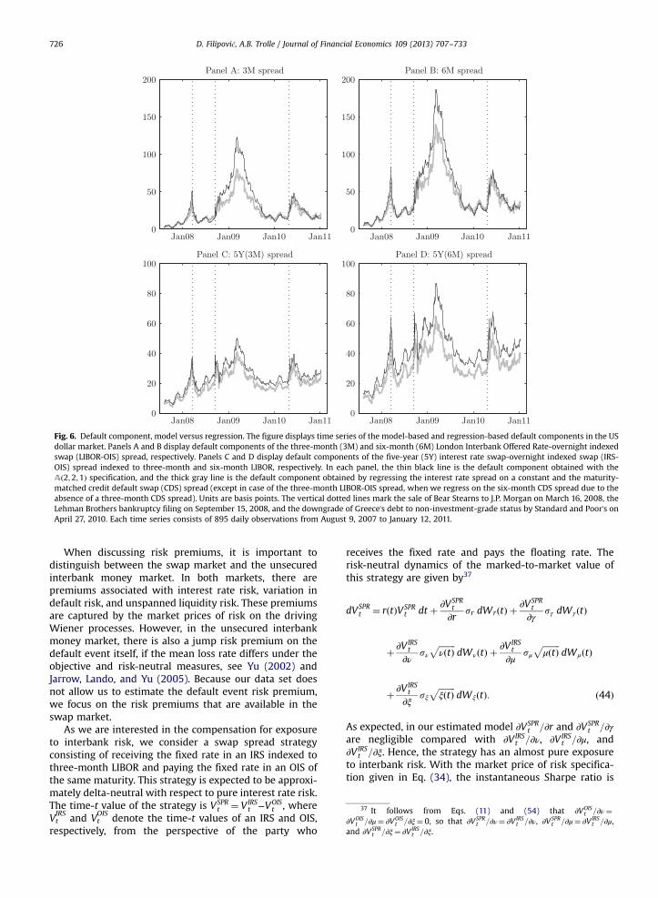
Fig. 6. Default component, model versus regression. The figure displays time series of the model-based and regression-based default components in the USdollar market. Panels A and B display default components of the three-month (3M) and six-month (6M) London Interbank Offered Rate-overnight indexedswap (LIBOR-OIS) spread, respectively. Panels C and D display default components of the five-year (5Y) interest rate swap-overnight indexed swap (IRS-OIS) spread indexed to three-month and six-month LIBOR, respectively. In each panel, the thin black line is the default component obtained with theAð2;2;1Þ specification, and the thick gray line is the default component obtained by regressing the interest rate spread on a constant and the maturity-matched credit default swap (CDS) spread (except in case of the three-month LIBOR-OIS spread, when we regress on the six-month CDS spread due to theabsence of a three-month CDS spread). Units are basis points. The vertical dotted lines mark the sale of Bear Stearns to J.P. Morgan on March 16, 2008, theLehman Brothers bankruptcy filing on September 15, 2008, and the downgrade of Greece's debt to non-investment-grade status by Standard and Poor's onApril 27, 2010. Each time series consists of 895 daily observations from August 9, 2007 to January 12, 2011.

37 It follows from Eqs. (11) and (54) that ∂VOISt =∂ν¼

∂VOISt =∂μ¼ ∂VOIS

t =∂ξ¼ 0, so that ∂VSPRt =∂ν¼ ∂VIRS

t =∂ν, ∂VSPRt =∂μ¼ ∂VIRS

t =∂μ,and ∂VSPR

t =∂ξ¼ ∂VIRSt =∂ξ.

D. Filipović, A.B. Trolle / Journal of Financial Economics 109 (2013) 707–733726

When discussing risk premiums, it is important todistinguish between the swap market and the unsecuredinterbank money market. In both markets, there arepremiums associated with interest rate risk, variation indefault risk, and unspanned liquidity risk. These premiumsare captured by the market prices of risk on the drivingWiener processes. However, in the unsecured interbankmoney market, there is also a jump risk premium on thedefault event itself, if the mean loss rate differs under theobjective and risk-neutral measures, see Yu (2002) andJarrow, Lando, and Yu (2005). Because our data set doesnot allow us to estimate the default event risk premium,we focus on the risk premiums that are available in theswap market.

As we are interested in the compensation for exposureto interbank risk, we consider a swap spread strategyconsisting of receiving the fixed rate in an IRS indexed tothree-month LIBOR and paying the fixed rate in an OIS ofthe same maturity. This strategy is expected to be approxi-mately delta-neutral with respect to pure interest rate risk.The time-t value of the strategy is VSPR

t ¼ VIRSt −VOIS

t , whereVtIRS

and VtOIS

denote the time-t values of an IRS and OIS,respectively, from the perspective of the party who

receives the fixed rate and pays the floating rate. Therisk-neutral dynamics of the marked-to-market value ofthis strategy are given by37

dVSPRt ¼ r tð ÞVSPR

t dt þ ∂VSPRt

∂rsr dWr tð Þ þ ∂VSPR

t

∂γsγ dWγ tð Þ

þ ∂VIRSt

∂νsν

ffiffiffiffiffiffiffiffiν tð Þ

pdWν tð Þ þ ∂VIRS

t

∂μsμ

ffiffiffiffiffiffiffiffiμ tð Þ

pdWμ tð Þ

þ ∂VIRSt

∂ξsξ

ffiffiffiffiffiffiffiffiξ tð Þ

pdWξ tð Þ: ð44Þ

As expected, in our estimated model ∂VSPRt =∂r and ∂VSPR

t =∂γare negligible compared with ∂VIRS

t =∂ν, ∂VIRSt =∂μ, and

∂VIRSt =∂ξ. Hence, the strategy has an almost pure exposure

to interbank risk. With the market price of risk specifica-tion given in Eq. (34), the instantaneous Sharpe ratio is

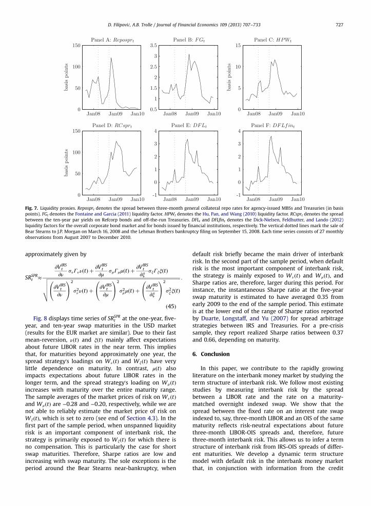
ffiÞ

:

Fig. 7. Liquidity proxies. Reposprt denotes the spread between three-month general collateral repo rates for agency-issued MBSs and Treasuries (in basispoints). FGt denotes the Fontaine and Garcia (2011) liquidity factor. HPWt denotes the Hu, Pan, and Wang (2010) liquidity factor. RCsprt denotes the spreadbetween the ten-year par yields on Refcorp bonds and off-the-run Treasuries. DFLt and DFLfint denotes the Dick-Nielsen, Feldhutter, and Lando (2012)liquidity factors for the overall corporate bond market and for bonds issued by financial institutions, respectively. The vertical dotted lines mark the sale ofBear Stearns to J.P. Morgan on March 16, 2008 and the Lehman Brothers bankruptcy filing on September 15, 2008. Each time series consists of 27 monthlyobservations from August 2007 to December 2010.

D. Filipović, A.B. Trolle / Journal of Financial Economics 109 (2013) 707–733 727

approximately given by

SRSPRt ≈

∂VIRSt

∂νsνΓνν tð Þ þ ∂VIRS

t

∂μsμΓμμ tð Þ þ ∂VIRS

t

∂ξsξΓξξ tð Þffiffiffiffiffiffiffiffiffiffiffiffiffiffiffiffiffiffiffiffiffiffiffiffiffiffiffiffiffiffiffiffiffiffiffiffiffiffiffiffiffiffiffiffiffiffiffiffiffiffiffiffiffiffiffiffiffiffiffiffiffiffiffiffiffiffiffiffiffiffiffiffiffiffiffiffiffiffiffiffiffiffiffiffiffiffiffiffiffiffiffiffiffiffiffiffiffiffiffiffiffiffiffiffiffiffiffiffiffiffiffi0@∂VIRS

t

∂ν

1A2

s2ν ν tð Þ þ0@∂VIRS

t

∂μ

1A2

s2μμ tð Þ þ0@∂VIRS

t

∂ξ

1A2

s2ξ ξ tð

vuuutð45Þ

Fig. 8 displays time series of SRSPRt at the one-year, five-

year, and ten-year swap maturities in the USD market(results for the EUR market are similar). Due to their fastmean-reversion, ν tð Þ and ξ tð Þ mainly affect expectationsabout future LIBOR rates in the near term. This impliesthat, for maturities beyond approximately one year, thespread strategy's loadings on Wν tð Þ and Wξ tð Þ have verylittle dependence on maturity. In contrast, μ tð Þ alsoimpacts expectations about future LIBOR rates in thelonger term, and the spread strategy's loading on Wμ tð Þincreases with maturity over the entire maturity range.The sample averages of the market prices of risk on Wν tð Þand Wμ tð Þ are −0.28 and −0.20, respectively, while we arenot able to reliably estimate the market price of risk onWξ tð Þ, which is set to zero (see end of Section 4.3). In thefirst part of the sample period, when unspanned liquidityrisk is an important component of interbank risk, thestrategy is primarily exposed to Wξ tð Þ for which there isno compensation. This is particularly the case for shortswap maturities. Therefore, Sharpe ratios are low andincreasing with swap maturity. The sole exceptions is theperiod around the Bear Stearns near-bankruptcy, when

default risk briefly became the main driver of interbankrisk. In the second part of the sample period, when defaultrisk is the most important component of interbank risk,the strategy is mainly exposed to Wν tð Þ and Wμ tð Þ, andSharpe ratios are, therefore, larger during this period. Forinstance, the instantaneous Sharpe ratio at the five-yearswap maturity is estimated to have averaged 0.35 fromearly 2009 to the end of the sample period. This estimateis at the lower end of the range of Sharpe ratios reportedby Duarte, Longstaff, and Yu (2007) for spread arbitragestrategies between IRS and Treasuries. For a pre-crisissample, they report realized Sharpe ratios between 0.37and 0.66, depending on maturity.

6. Conclusion

In this paper, we contribute to the rapidly growingliterature on the interbank money market by studying theterm structure of interbank risk. We follow most existingstudies by measuring interbank risk by the spreadbetween a LIBOR rate and the rate on a maturity-matched overnight indexed swap. We show that thespread between the fixed rate on an interest rate swapindexed to, say, three-month LIBOR and an OIS of the samematurity reflects risk-neutral expectations about futurethree-month LIBOR-OIS spreads and, therefore, futurethree-month interbank risk. This allows us to infer a termstructure of interbank risk from IRS-OIS spreads of differ-ent maturities. We develop a dynamic term structuremodel with default risk in the interbank money marketthat, in conjunction with information from the credit

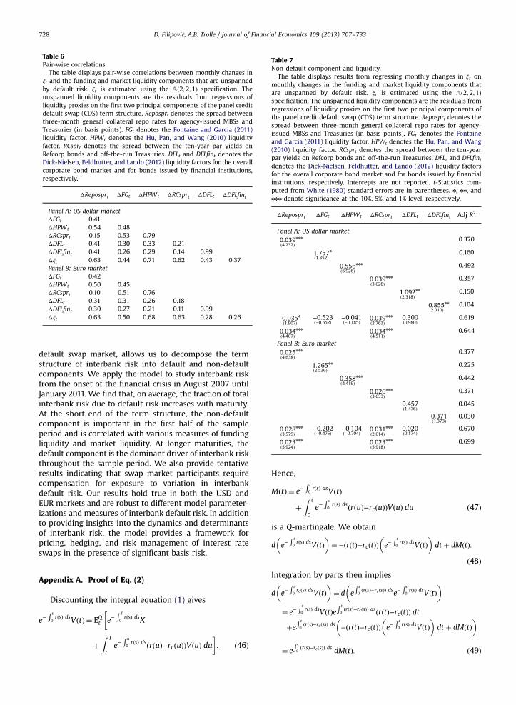
Table 7Non-default component and liquidity.

The table displays results from regressing monthly changes in ξt onmonthly changes in the funding and market liquidity components thatare unspanned by default risk. ξt is estimated using the Að2;2;1Þspecification. The unspanned liquidity components are the residuals fromregressions of liquidity proxies on the first two principal components ofthe panel credit default swap (CDS) term structure. Reposprt denotes thespread between three-month general collateral repo rates for agency-issued MBSs and Treasuries (in basis points). FGt denotes the Fontaineand Garcia (2011) liquidity factor. HPWt denotes the Hu, Pan, and Wang(2010) liquidity factor. RCsprt denotes the spread between the ten-yearpar yields on Refcorp bonds and off-the-run Treasuries. DFLt and DFLfintdenotes the Dick-Nielsen, Feldhutter, and Lando (2012) liquidity factorsfor the overall corporate bond market and for bonds issued by financialinstitutions, respectively. Intercepts are not reported. t-Statistics com-puted from White (1980) standard errors are in parentheses. n, nn, andnnn denote significance at the 10%, 5%, and 1% level, respectively.

ΔReposprt ΔFGt ΔHPWt ΔRCsprt ΔDFLt ΔDFLfint Adj R2

Panel A: US dollar market0:039ð4:232Þ

nnn 0.370

1:757ð1:852Þ

n 0.160

0:556ð6:926Þ

nnn 0.492

0:039ð3:628Þ

nnn 0.357

1:092ð2:318Þ

nn 0.150

0:855ð2:010Þ

nn 0.104

0:035ð1:907Þ

n −0:523ð−0:652Þ

−0:041ð−0:185Þ 0:039

ð2:763Þnnn 0:300

ð0:980Þ0.619

0:034ð4:407Þ

nnn 0:034ð4:511Þ

nnn 0.644

Panel B: Euro market0:025ð4:638Þ

nnn 0.377

1:265ð2:536Þ

nn 0.225

0:358ð4:419Þ

nnn 0.442

0:026ð3:633Þ

nnn 0.371

0:457ð1:476Þ

0.045

0:371ð1:373Þ

0.030

0:028ð3:579Þ

nnn −0:202ð−0:475Þ

−0:104ð−0:704Þ 0:031

ð2:614Þnnn 0:020

ð0:174Þ0.670

0:023ð5:924Þ

nnn 0:023ð5:918Þ

nnn 0.699

Table 6Pair-wise correlations.

The table displays pair-wise correlations between monthly changes inξt and the funding and market liquidity components that are unspannedby default risk. ξt is estimated using the Að2;2;1Þ specification. Theunspanned liquidity components are the residuals from regressions ofliquidity proxies on the first two principal components of the panel creditdefault swap (CDS) term structure. Reposprt denotes the spread betweenthree-month general collateral repo rates for agency-issued MBSs andTreasuries (in basis points). FGt denotes the Fontaine and Garcia (2011)liquidity factor. HPWt denotes the Hu, Pan, and Wang (2010) liquidityfactor. RCsprt denotes the spread between the ten-year par yields onRefcorp bonds and off-the-run Treasuries. DFLt and DFLfint denotes theDick-Nielsen, Feldhutter, and Lando (2012) liquidity factors for the overallcorporate bond market and for bonds issued by financial institutions,respectively.

ΔReposprt ΔFGt ΔHPWt ΔRCsprt ΔDFLt ΔDFLfint

Panel A: US dollar marketΔFGt 0.41ΔHPWt 0.54 0.48ΔRCsprt 0.15 0.53 0.79ΔDFLt 0.41 0.30 0.33 0.21ΔDFLfint 0.41 0.26 0.29 0.14 0.99Δξt 0.63 0.44 0.71 0.62 0.43 0.37Panel B: Euro marketΔFGt 0.42ΔHPWt 0.50 0.45ΔRCsprt 0.10 0.51 0.76ΔDFLt 0.31 0.31 0.26 0.18ΔDFLfint 0.30 0.27 0.21 0.11 0.99Δξt 0.63 0.50 0.68 0.63 0.28 0.26

D. Filipović, A.B. Trolle / Journal of Financial Economics 109 (2013) 707–733728

default swap market, allows us to decompose the termstructure of interbank risk into default and non-defaultcomponents. We apply the model to study interbank riskfrom the onset of the financial crisis in August 2007 untilJanuary 2011. We find that, on average, the fraction of totalinterbank risk due to default risk increases with maturity.At the short end of the term structure, the non-defaultcomponent is important in the first half of the sampleperiod and is correlated with various measures of fundingliquidity and market liquidity. At longer maturities, thedefault component is the dominant driver of interbank riskthroughout the sample period. We also provide tentativeresults indicating that swap market participants requirecompensation for exposure to variation in interbankdefault risk. Our results hold true in both the USD andEUR markets and are robust to different model parameter-izations and measures of interbank default risk. In additionto providing insights into the dynamics and determinantsof interbank risk, the model provides a framework forpricing, hedging, and risk management of interest rateswaps in the presence of significant basis risk.

Appendix A. Proof of Eq. (2)

Discounting the integral equation (1) gives

e−R t

0r sð Þ dsV tð Þ ¼ EQt e−

R T

0r sð Þ dsX

�

þZ T

te−R u

0r sð Þ ds r uð Þ−rc uð Þð ÞV uð Þ du

�: ð46Þ

Hence,

M tð Þ ¼ e−R t

0r sð Þ dsV tð Þ

þZ t

0e−R u

0r sð Þ ds r uð Þ−rc uð Þð ÞV uð Þ du ð47Þ

is a Q-martingale. We obtain

d e−R t

0r sð Þ dsV tð Þ

� �¼− r tð Þ−rc tð Þð Þ e−

R t

0r sð Þ dsV tð Þ

� �dt þ dM tð Þ:

ð48ÞIntegration by parts then implies

d e−R t

0rc sð Þ dsV tð Þ

� �¼ d e

R t

0r sð Þ−rc sð Þð Þ dse−

R t

0r sð Þ dsV tð Þ

� �¼ e−

R t

0r sð Þ dsV tð Þe

R t

0r sð Þ−rc sð Þð Þ ds r tð Þ−rc tð Þð Þ dt

þeR t

0r sð Þ−rc sð Þð Þ ds − r tð Þ−rc tð Þð Þ e−

R t

0r sð Þ dsV tð Þ

� �dt þ dM tð Þ

� �

¼ eR t

0r sð Þ−rc sð Þð Þ ds dM tð Þ: ð49Þ

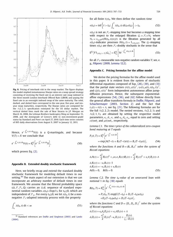
Fig. 8. Pricing of interbank risk in the swap market. The figure displaysthe model-implied instantaneous Sharpe ratios on a swap spread strategyconsisting of receiving the fixed rate in an interest rate swap indexed tothe three-month London Interbank Offered Rate (LIBOR) and paying thefixed rate in an overnight indexed swap of the same maturity. The solid,dashed, and dotted lines correspond to the one-year, five-year, and ten-year swap maturities, respectively. The Sharpe ratios are computed forthe Að2;2;1Þ specification estimated for the US dollar market. Thevertical dotted lines mark the sale of Bear Stearns to J.P. Morgan onMarch 16, 2008, the Lehman Brothers bankruptcy filing on September 15,2008, and the downgrade of Greece's debt to non-investment-gradestatus by Standard and Poor's on April 27, 2010. Each time series consistsof 895 daily observations from August 9, 2007 to January 12, 2011.

D. Filipović, A.B. Trolle / Journal of Financial Economics 109 (2013) 707–733 729

Hence, e−R t

0rc sð Þ dsV tð Þ is a Q-martingale, and because

V Tð Þ ¼ X we conclude that

e−R t

0rc sð Þ dsV tð Þ ¼ EQt e−

R T

0rc sð Þ dsX

� �; ð50Þ

which proves Eq. (2).

Appendix B. Extended doubly stochastic framework

Here, we briefly recap and extend the standard doublystochastic framework for modeling default times in oursetting.38 The main aspect of our extension is that we canincorporate an arbitrary number of default times in oneframework. We assume that the filtered probability spaceΩ;F ;F t ;Qð Þ carries an i.i.d. sequence of standard expo-nential random variables ε t0ð Þ∼Exp 1ð Þ, for t0≥0, which areindependent of F∞. For every t0≥0, we let λ t0; tð Þ be a non-negative F t-adapted intensity process with the propertyZ t

t0λ t0; sð Þ dso∞ ð51Þ

38 Standard references are Duffie and Singleton (2003) and Lando(2004).

for all finite t≥t0. We then define the random time

τ t0ð Þ ¼ inf t4t0jZ t

t0λ t0; sð Þ ds≥ε t0ð Þ

� �4t0: ð52Þ

τ t0ð Þ is not an F t-stopping time but becomes a stopping timewith respect to the enlarged filtration Gt ¼F t∨Ht whereHt ¼ ∨t0≥0s H t0; sð Þjs≤tð Þ is the filtration generated by allτ t0ð Þ-indicator processes H t0; tð Þ ¼ 1fτ t0ð Þ≤tg. The Gt-stoppingtimes τ t0ð Þ are then F t-doubly stochastic in the sense that

EQ Y1fτ t0ð Þ4TgjGt0

� ¼ EQt0 Ye

−R T

t0λ t0 ;sð Þ ds

" #ð53Þ

for all F T-measurable non-negative randomvariables Y; see, e.g., Filipović (2009, Lemma 12.2).

Appendix C. Pricing formulas for the affine model

We derive the pricing formulas for the affine model usedin this paper. It is evident from the system of stochasticdifferential equations composed of Eqs. (26), (30), and (33)that the partial state vectors r tð Þ; γ tð Þð Þ⊤, ν tð Þ; μ tð Þ; λ t0; tð Þð Þ⊤,and ξ tð Þ; ϵ tð Þð Þ⊤ form independent autonomous affine jump-diffusion processes. Hence, the subsequent exponential-affine expressions (54), (56), and (62) follow directly fromthe general affine transform formula in Duffie, Filipovic, andSchachermayer (2003, Section 2) and the fact thatrc tð Þ ¼ r tð Þ þ Λ, see Eq. (21). The following formulas are forthe full A 2;2;2ð Þ model. The nested versions, A 2;2;1ð Þ andA 2;1;1ð Þ, are obtained by setting the respective modelparameters, κϵ; θϵ; sϵ and κμ; θμ; sμ, equal to zero and settingϵ tð Þ≡θξ and μ tð Þ≡θν, respectively.

Lemma C.1. The time t price of the collateralized zero-couponbond maturing at T equals

Pc t; Tð Þ ¼ EQt e−R T

trc sð Þ ds

� �¼ exp A T−tð Þ þ Br T−tð Þr tð Þ þ Bγ T−tð Þγ tð Þ�

; ð54Þ

where the functions A and B¼ Br ;BΛð Þ⊤ solve the system ofRiccati equations

∂τA τð Þ ¼ s2r2Br τð Þ2 þ ρsrsγBr τð ÞBγ τð Þ þ s2γ

2Bγ τð Þ2 þ κγθγBγ τð Þ−Λ

∂τBr τð Þ ¼−κrBr τð Þ−1∂τBγ τð Þ ¼−κγBγ τð Þ þ κrBr τð ÞA 0ð Þ ¼ 0; B 0ð Þ ¼ 0: ð55Þ

Lemma C.2. The time t0-value of an unsecured loan withnotional 1 in Eq. (18) equals

B t0; Tð Þ ¼ EQt0 e−R T

t0r sð Þþλ t0 ;sð Þð Þ ds

" #¼ Pc t0; Tð Þ exp C T−t0ð Þ þ Dν T−t0ð Þν t0ð Þ½þDμ T−t0ð Þμ t0ð Þ þ Dλ T−t0ð ÞΛ ; ð56Þ

where the functions C and D¼ Dν;Dμ;Dλ

� �⊤ solve the systemof Riccati equations

∂τC τð Þ ¼ κμθμDμ τð Þ þ κλΛDλ τð Þ þ Λ

∂τDν τð Þ ¼ s2ν2Dν τð Þ2−κνDν τð Þ þ Dλ τð Þ

ζλ−Dλ τð Þ

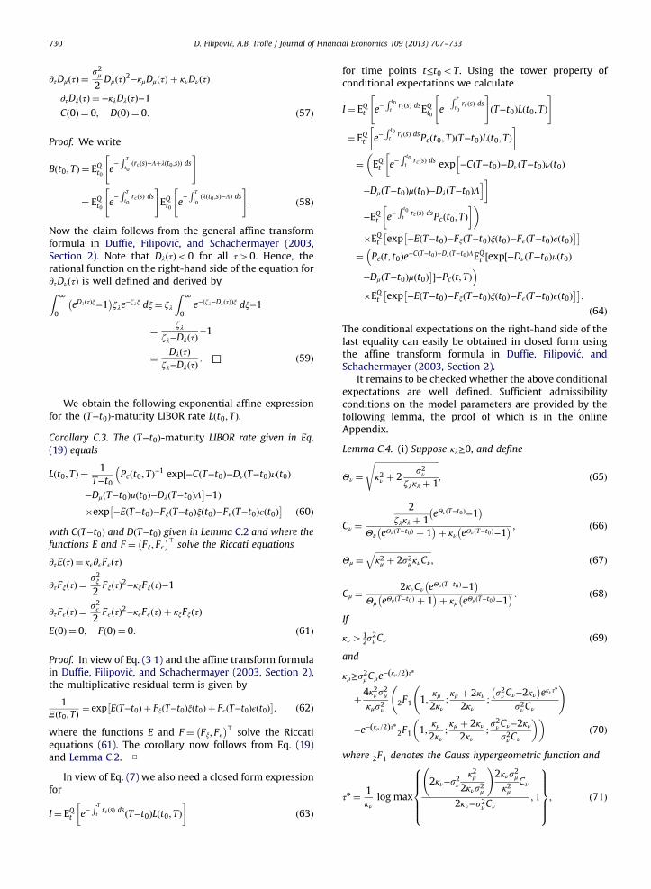
D. Filipović, A.B. Trolle / Journal of Financial Economics 109 (2013) 707–733730

∂τDμ τð Þ ¼ s2μ2Dμ τð Þ2−κμDμ τð Þ þ κνDν τð Þ

∂τDλ τð Þ ¼−κλDλ τð Þ−1C 0ð Þ ¼ 0; D 0ð Þ ¼ 0: ð57Þ

Proof. We write

B t0; Tð Þ ¼ EQt0 e−R T

t0rc sð Þ−Λþλ t0 ;sð Þð Þ ds

" #

¼ EQt0 e−R T

t0rc sð Þ ds

" #EQt0 e

−R T

t0λ t0 ;sð Þ−Λð Þ ds

" #: ð58Þ

Now the claim follows from the general affine transformformula in Duffie, Filipovic, and Schachermayer (2003,Section 2). Note that Dλ τð Þo0 for all τ40. Hence, therational function on the right-hand side of the equation for∂τDν τð Þ is well defined and derived byZ ∞

0eDλ τð Þξ−1� �

ζλe−ζλξ dξ¼ ζλ

Z ∞

0e− ζλ−Dλ τð Þð Þξ dξ−1

¼ ζλζλ−Dλ τð Þ−1

¼ Dλ τð Þζλ−Dλ τð Þ : □ ð59Þ

We obtain the following exponential affine expressionfor the T−t0ð Þ-maturity LIBOR rate L t0; Tð Þ.

Corollary C.3. The T−t0ð Þ-maturity LIBOR rate given in Eq.(19) equals

L t0; Tð Þ ¼ 1T−t0

Pc t0; Tð Þ−1 exp −C T−t0ð Þ−Dν T−t0ð Þν t0ð Þ½

−Dμ T−t0ð Þμ t0ð Þ−Dλ T−t0ð ÞΛ −1Þ�exp −E T−t0ð Þ−Fξ T−t0ð Þξ t0ð Þ−Fϵ T−t0ð Þϵ t0ð Þ� ð60Þ

with C T−t0ð Þ and D T−t0ð Þ given in Lemma C.2 and where thefunctions E and F ¼ Fξ; Fϵ

� �⊤ solve the Riccati equations

∂τE τð Þ ¼ κϵθϵFϵ τð Þ

∂τFξ τð Þ ¼ s2ξ2Fξ τð Þ2−κξFξ τð Þ−1

∂τFϵ τð Þ ¼ s2ϵ2Fϵ τð Þ2−κϵFϵ τð Þ þ κξFξ τð Þ

E 0ð Þ ¼ 0; F 0ð Þ ¼ 0: ð61Þ

Proof. In view of Eq. (3 1) and the affine transform formulain Duffie, Filipovic, and Schachermayer (2003, Section 2),the multiplicative residual term is given by

1Ξ t0; Tð Þ ¼ exp E T−t0ð Þ þ Fξ T−t0ð Þξ t0ð Þ þ Fϵ T−t0ð Þϵ t0ð Þ�

; ð62Þ

where the functions E and F ¼ Fξ; Fϵ� �⊤ solve the Riccati

equations (61). The corollary now follows from Eq. (19)and Lemma C.2. □

In view of Eq. (7) we also need a closed form expressionfor

I ¼ EQt e−R T

trc sð Þ ds T−t0ð ÞL t0; Tð Þ

� �ð63Þ

for time points t≤t0oT . Using the tower property ofconditional expectations we calculate

I ¼ EQt e−R t0t

rc sð Þ dsEQt0 e−R T

t0rc sð Þ ds

" #T−t0ð ÞL t0; Tð Þ

" #

¼ EQt e−R t0t

rc sð Þ dsPc t0; Tð Þ T−t0ð ÞL t0; Tð Þ� �

¼ EQt

�e−R t0t

rc sð Þ ds exph−C T−t0ð Þ−Dν T−t0ð Þν t0ð Þ

�−Dμ T−t0ð Þμ t0ð Þ−Dλ T−t0ð ÞΛ

i�−EQ

t e−R t0t

rc sð Þ dsPc t0; Tð Þ� ��

�EQt exp −E T−t0ð Þ−Fξ T−t0ð Þξ t0ð Þ−Fϵ T−t0ð Þϵ t0ð Þ� � ¼Pc t; t0ð Þe−C T−t0ð Þ−Dλ T−t0ð ÞΛEQt exp −Dν T−t0ð Þν t0ð Þ½½

−Dμ T−t0ð Þμ t0ð Þ �−Pc t; Tð Þ

�EQt exp −E T−t0ð Þ−Fξ T−t0ð Þξ t0ð Þ−Fϵ T−t0ð Þϵ t0ð Þ� � :

ð64ÞThe conditional expectations on the right-hand side of thelast equality can easily be obtained in closed form usingthe affine transform formula in Duffie, Filipovic, andSchachermayer (2003, Section 2).

It remains to be checked whether the above conditionalexpectations are well defined. Sufficient admissibilityconditions on the model parameters are provided by thefollowing lemma, the proof of which is in the onlineAppendix.

Lemma C.4. (i) Suppose κλ≥0, and define

Θν ¼ffiffiffiffiffiffiffiffiffiffiffiffiffiffiffiffiffiffiffiffiffiffiffiffiffiffiffiffiffiffiffiκ2ν þ 2

s2νζλκλ þ 1

s; ð65Þ

Cν ¼2

ζλκλ þ 1eΘν T−t0ð Þ−1� �

Θν eΘν T−t0ð Þ þ 1� �þ κν eΘν T−t0ð Þ−1

� � ; ð66Þ

Θμ ¼ffiffiffiffiffiffiffiffiffiffiffiffiffiffiffiffiffiffiffiffiffiffiffiffiffiffiffiκ2μ þ 2s2μκνCν

q; ð67Þ

Cμ ¼2κνCν eΘμ T−t0ð Þ−1

� �Θμ eΘμ T−t0ð Þ þ 1� �þ κμ eΘμ T−t0ð Þ−1

� � : ð68Þ

If

κν412s

2νCν ð69Þ

and

κμ≥s2μCμe− κμ=2ð Þτn

þ4κ2νs2μ

κμs2ν2F1 1;

κμ2κν

;κμ þ 2κν

2κν;s2νCν−2κν� �

eκντn

s2νCν

!

−e− κμ=2ð Þτn2F1 1;

κμ2κν

;κμ þ 2κν

2κν;s2νCν−2κν

s2νCν

� ��ð70Þ

where 2F1 denotes the Gauss hypergeometric function and

τn ¼ 1κν

log max

2κν−s2νκ2μ

2κνs2μ

!2κνs2μκ2μ

Cν

2κν−s2νCν;1

8>>>><>>>>:

9>>>>=>>>>;; ð71Þ

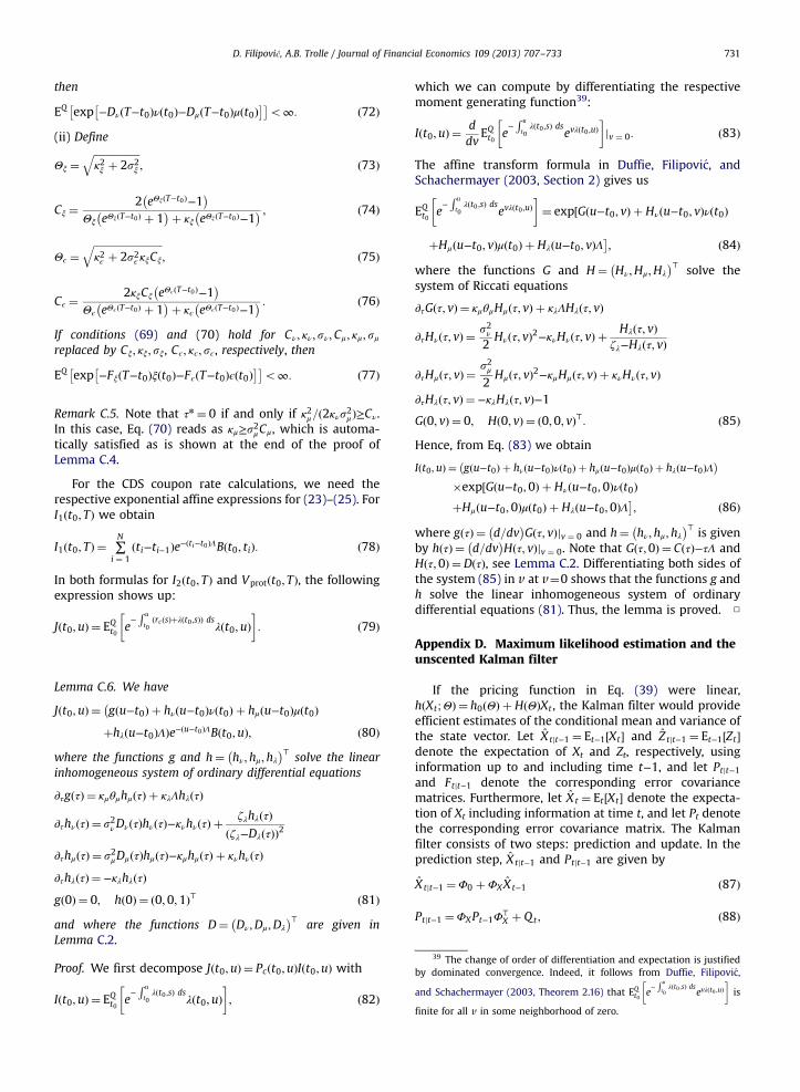
39 The change of order of differentiation and expectation is justifiedby dominated convergence. Indeed, it follows from Duffie, Filipovic,

and Schachermayer (2003, Theorem 2.16) that EQt0 e−R u

t0λ t0 ;sð Þ ds

evλ t0 ;uð Þ� �

is

finite for all v in some neighborhood of zero.

D. Filipović, A.B. Trolle / Journal of Financial Economics 109 (2013) 707–733 731

then

EQ exp −Dν T−t0ð Þν t0ð Þ−Dμ T−t0ð Þμ t0ð Þ� � o∞: ð72Þ

(ii) Define

Θξ ¼ffiffiffiffiffiffiffiffiffiffiffiffiffiffiffiffiffiffiκ2ξ þ 2s2ξ

q; ð73Þ

Cξ ¼2 eΘξ T−t0ð Þ−1� �

Θξ eΘξ T−t0ð Þ þ 1� �þ κξ eΘξ T−t0ð Þ−1

� � ; ð74Þ

Θϵ ¼ffiffiffiffiffiffiffiffiffiffiffiffiffiffiffiffiffiffiffiffiffiffiffiffiffiffiffiκ2ϵ þ 2s2ϵ κξCξ

q; ð75Þ

Cϵ ¼2κξCξ eΘϵ T−t0ð Þ−1

� �Θϵ eΘϵ T−t0ð Þ þ 1� �þ κϵ eΘϵ T−t0ð Þ−1

� � : ð76Þ

If conditions (69) and (70) hold for Cν; κν; sν;Cμ; κμ;sμreplaced by Cξ; κξ; sξ, Cϵ; κϵ; sϵ, respectively, then

EQ exp −Fξ T−t0ð Þξ t0ð Þ−Fϵ T−t0ð Þϵ t0ð Þ� � o∞: ð77Þ

Remark C.5. Note that τn ¼ 0 if and only if κ2μ=ð2κνs2μÞ≥Cν.In this case, Eq. (70) reads as κμ≥s2μCμ, which is automa-tically satisfied as is shown at the end of the proof ofLemma C.4.

For the CDS coupon rate calculations, we need therespective exponential affine expressions for (23)–(25). ForI1 t0; Tð Þ we obtain

I1 t0; Tð Þ ¼ ∑N

i ¼ 1ti−ti−1ð Þe− ti−t0ð ÞΛB t0; tið Þ: ð78Þ

In both formulas for I2 t0; Tð Þ and Vprot t0; Tð Þ, the followingexpression shows up:

J t0;uð Þ ¼ EQt0 e−R u

t0rc sð Þþλ t0 ;sð Þð Þ ds

λ t0;uð Þ� �

: ð79Þ

Lemma C.6. We have

J t0;uð Þ ¼ g u−t0ð Þ þ hν u−t0ð Þν t0ð Þ þ hμ u−t0ð Þμ t0ð Þ�þhλ u−t0ð ÞΛÞe− u−t0ð ÞΛB t0;uð Þ; ð80Þ

where the functions g and h¼ hν;hμ;hλ� �⊤ solve the linear

inhomogeneous system of ordinary differential equations

∂τg τð Þ ¼ κμθμhμ τð Þ þ κλΛhλ τð Þ

∂τhν τð Þ ¼ s2νDν τð Þhν τð Þ−κνhν τð Þ þ ζλhλ τð Þζλ−Dλ τð Þð Þ2

∂τhμ τð Þ ¼ s2μDμ τð Þhμ τð Þ−κμhμ τð Þ þ κνhν τð Þ∂τhλ τð Þ ¼ −κλhλ τð Þg 0ð Þ ¼ 0; h 0ð Þ ¼ 0;0;1ð Þ⊤ ð81Þ

and where the functions D¼ Dν;Dμ;Dλ

� �⊤ are given inLemma C.2.

Proof. We first decompose J t0;uð Þ ¼ Pc t0;uð ÞI t0;uð Þ with

I t0;uð Þ ¼ EQt0 e−R u

t0λ t0 ;sð Þ ds

λ t0;uð Þ� �

; ð82Þ

which we can compute by differentiating the respectivemoment generating function39:

I t0;uð Þ ¼ ddv

EQt0 e−R u

t0λ t0 ;sð Þ ds

evλ t0 ;uð Þ� �

jv ¼ 0: ð83Þ

The affine transform formula in Duffie, Filipovic, andSchachermayer (2003, Section 2) gives us

EQt0 e−R u

t0λ t0 ;sð Þ ds

evλ t0 ;uð Þ� �

¼ exp G u−t0; vð Þ þ Hν u−t0; vð Þν t0ð Þ½

þHμ u−t0; vð Þμ t0ð Þ þ Hλ u−t0; vð ÞΛ ; ð84Þ

where the functions G and H¼ Hν;Hμ;Hλ

� �⊤ solve thesystem of Riccati equations

∂τG τ; vð Þ ¼ κμθμHμ τ; vð Þ þ κλΛHλ τ; vð Þ

∂τHν τ; vð Þ ¼ s2ν2Hν τ; vð Þ2−κνHν τ; vð Þ þ Hλ τ; vð Þ

ζλ−Hλ τ; vð Þ

∂τHμ τ; vð Þ ¼ s2μ2Hμ τ; vð Þ2−κμHμ τ; vð Þ þ κνHν τ; vð Þ

∂τHλ τ; vð Þ ¼−κλHλ τ; vð Þ−1G 0; vð Þ ¼ 0; H 0; vð Þ ¼ 0;0; vð Þ⊤: ð85Þ

Hence, from Eq. (83) we obtain

I t0;uð Þ ¼ g u−t0ð Þ þ hν u−t0ð Þν t0ð Þ þ hμ u−t0ð Þμ t0ð Þ þ hλ u−t0ð ÞΛ� ��exp G u−t0;0ð Þ þ Hν u−t0;0ð Þν t0ð Þ½þHμ u−t0;0ð Þμ t0ð Þ þ Hλ u−t0;0ð ÞΛ ; ð86Þ

where g τð Þ ¼ d=dv� �

G τ; vð Þjv ¼ 0 and h¼ hν;hμ;hλ� �⊤ is given

by h τð Þ ¼ d=dv� �

H τ; vð Þjv ¼ 0. Note that G τ;0ð Þ ¼ C τð Þ−τΛ andH τ;0ð Þ ¼D τð Þ, see Lemma C.2. Differentiating both sides ofthe system (85) in v at v¼0 shows that the functions g andh solve the linear inhomogeneous system of ordinarydifferential equations (81). Thus, the lemma is proved. □

Appendix D. Maximum likelihood estimation and theunscented Kalman filter

If the pricing function in Eq. (39) were linear,h Xt ;Θð Þ ¼ h0 Θð Þ þ H Θð ÞXt , the Kalman filter would provideefficient estimates of the conditional mean and variance ofthe state vector. Let X tjt−1 ¼ Et−1 Xt½ � and Z tjt−1 ¼ Et−1 Zt½ �denote the expectation of Xt and Zt, respectively, usinginformation up to and including time t−1, and let Ptjt−1and Ftjt−1 denote the corresponding error covariancematrices. Furthermore, let X t ¼ Et Xt½ � denote the expecta-tion of Xt including information at time t, and let Pt denotethe corresponding error covariance matrix. The Kalmanfilter consists of two steps: prediction and update. In theprediction step, X tjt−1 and Ptjt−1 are given by

X tjt−1 ¼Φ0 þΦXX t−1 ð87Þ

Ptjt−1 ¼ΦXPt−1Φ⊤X þ Qt ; ð88Þ

;2L;

D. Filipović, A.B. Trolle / Journal of Financial Economics 109 (2013) 707–733732

and Z tjt−1 and Ftjt−1 are in turn given by

Z tjt−1 ¼ h X tjt−1;Θ

ð89Þ

Ftjt−1 ¼HPtjt−1H⊤ þ Σ: ð90Þ

In the update step, the estimate of the state vector isrefined based on the difference between predicted andobserved quantities, with X t ¼ Et Xt½ � and Pt given by

X t ¼ X tjt−1 þWt Zt−Z tjt−1

ð91Þ

Pt ¼ Ptjt−1−WtFtjt−1W⊤t ; ð92Þ

where

Wt ¼ Ptjt−1H⊤F−1tjt−1 ð93Þ

is the covariance between pricing and filtering errors.In our setting, the pricing function is nonlinear for

all the instruments included in the estimation, and theKalman filter has to be modified. Nonlinear statespace systems have traditionally been handled with theextended Kalman filter, which effectively linearizes themeasure equation around the predicted state. However, inrecent years the unscented Kalman filter has emerged as avery attractive alternative. Instead of approximating themeasurement equation, it uses the true nonlinear mea-surement equation and instead approximates the distribu-tion of the state vector with a deterministically chosen setof sample points, called sigma points, that completelycapture the true mean and covariance of the state vector.When propagated through the nonlinear pricing function,the sigma points capture the mean and covariance of thedata accurately to the second order (third order for trueGaussian states) for any nonlinearity.40

More specifically, a set of 2L+1 sigma points andassociated weights are selected according to the followingscheme:

X 0tjt−1 ¼ X tjt−1; w0 ¼ κ

Lþ κ

X itjt−1 ¼ X tjt−1 þ

ffiffiffiffiffiffiffiffiffiffiffiffiffiffiffiffiffiffiffiffiffiffiffiffiffiLþ κð ÞPtjt−1

q �i; wi ¼ 1

2 Lþ κð Þ ; i¼ 1;…; L�

X itjt−1 ¼ X tjt−1−

ffiffiffiffiffiffiffiffiffiffiffiffiffiffiffiffiffiffiffiffiffiffiffiffiffiLþ κð ÞPtjt−1

q �i; wi ¼ 1

2 Lþ κð Þ ; i¼ Lþ 1;…�

ð94Þ

where L is the dimension of X tjt−1, κ is a scaling parameter,wi is the weight associated with the ith sigma-point, andffiffiffiffiffiffiffiffiffiffiffiffiffiffiffiffiffiffiffiffiffiffiffiffiffi

Lþ κð ÞPtjt−1p� �

i is the ith column of the matrix squareroot. Then, in the prediction step, Eqs. (89) and (90) arereplaced by

Z tjt−1 ¼ ∑2L

i ¼ 0wih X i

tjt−1;Θ

ð95Þ

40 For comparison, the extended Kalman filter estimates the meanand covariance accurately to the first order. The computational costs ofthe extended Kalman filter and the unscented Kalman filter are of thesame order of magnitude.

Ftjt−1 ¼ ∑2L

i ¼ 0wi h X i

tjt−1;Θ

−Z tjt−1

h X itjt−1;Θ

−Z tjt−1

⊤þ Σ:

ð96ÞThe update step is still given by Eqs. (91) and (92), butwith Wt computed as

Wt ¼ ∑2L

i ¼ 0wi X i

tjt−1−X tjt−1

h X itjt−1;Θ

−Z tjt−1

⊤F−1tjt−1:

ð97Þ

When implementing the Kalman filter, we follow usualpractice and initialize X t and Pt at their unconditionalvalues. Another implementation issue is that a subset ofthe state variables (νt , μt , ξt , and ϵt) are restricted to benon-negative, but because this is not taken into account inthe update step (91), negative values could occur. In thesecases, we replace negative values in X t by zeros. Thissolution appears to be fairly standard in the empirical termstructure literature and is discussed in detail in Chen andScott (2003).

In terms of maximizing the log-likelihood function, weinitially apply the Nelder-Mead algorithm and later switchto the gradient-based BFGS (Broyden-Fletcher-Goldfarb-Shanno) algorithm. The optimization is repeated withseveral different plausible initial parameter guesses, tominimize the risk of not reaching the global optimum.

Appendix E. Supplementary data

Supplementary data associated with this article can befound in the online version at http://dx.doi.org.10.1016/j.jfineco.2013.03.014.

References

Acharya, V., Gromb, D., Yorulmazer, T., 2012. Imperfect competition in theinterbank market for liquidity as a rationale for central banking.American Economic Journal: Macroeconomics 4, 184–217.

Acharya, V., Shin, H., Yorulmazer, T., 2011. Crisis resolution and bankliquidity. Review of Financial Studies 24, 2166–2205.

Acharya, V., Skeie, D., 2011. A model of liquidity hoarding and termpremia in interbank markets. Journal of Monetary Economics 58,436–447.

Afonso, G., Kovner, A., Schoar, A., 2009. Stressed, not frozen: the federalfunds market in the financial crisis. Unpublished working paper.Federal Reserve Bank of New York and Massachusetts Institute ofTechnology.

Allen, F., Carletti, E., Gale, D., 2009. Interbank market liquidity and centralbank intervention. Journal of Monetary Economics 56, 639–652.

Andersen, L., Piterbarg, V., 2010. Interest Rate Modeling. Atlantic FinancialPress, New York, NY.

Ang, A., Longstaff, F., 2011. Systemic sovereign credit risk: lessons fromthe US and Europe. Unpublished working paper. Columbia BusinessSchool and University of California, Los Angeles.

Angelini, P., Nobili, A., Picillo, M., 2009. The interbank market after August2007: what has changed and why? Unpublished working paper. Bankof Italy.

Arora, N., Gandhi, P., Longstaff, F., 2012. Counterparty credit risk and thecredit default swap market. Journal of Financial Economics 103,280–293.

Bartolini, L., Hilton, S., Sundaresan, S., Tonetti, C., 2011. Collateral valuesby asset class: evidence from primary securities dealers. Review ofFinancial Studies 24, 248–278.

Bauer, M., 2011. Bayesian estimation of dynamic term structure modelsunder restrictions on risk pricing. Unpublished working paper.Federal Reserve Bank of San Francisco.

D. Filipović, A.B. Trolle / Journal of Financial Economics 109 (2013) 707–733 733

Beber, A., Brandt, M., Kavajecz, K., 2009. Flight-to-quality or flight-to-liquidity? Evidence from the euro-area bond market. Review ofFinancial Studies 22, 925–957.

Bianchetti, M., 2009. Two curves, one price: pricing and hedging interestrate derivatives decoupling forwarding and discounting yield curves.Unpublished working paper. Banca Intesa San Paolo.

Blanco, R., Brennan, S., Marsh, I., 2005. An empirical analysis of thedynamic relation between investment-grade bonds and credit defaultswaps. Journal of Finance 60, 2255–2281.

Brunnermeier, M., Pedersen, L., 2009. Market liquidity and fundingliquidity. Review of Financial Studies 22, 2201–2238.

Chen, R., Scott, L., 2003. Multifactor Cox–Ingersoll–Ross models of theterm structure: estimates and tests from a Kalman filter model.Journal of Real Estate Finance and Economics 27, 143–172.

Christoffersen, P., Jacobs, K., Karoui, L., Mimouni, K., 2009. Nonlinearfiltering in affine term structure models: evidence from the termstructure of swap rates. Unpublished working paper. McGill Univer-sity and Goldman Sachs.

Collin-Dufresne, P., Solnik, B., 2001. On the term structure of defaultpremia in the swap and LIBOR markets. Journal of Finance 56,1095–1116.

Copeland, A., Martin, A., Walker, M., 2010. The tri-party repo marketbefore the 2010 reforms. Unpublished working paper. Federal ReserveBank of New York.

Dai, Q., Singleton, K., 2000. Specification analysis of affine term structuremodels. Journal of Finance 55, 1943–1978.

Dai, Q., Singleton, K., 2002. Expectations puzzles, time-varying riskpremia, and affine models of the term structure. Journal of FinancialEconomics 63, 415–442.

Diamond, D., Rajan, R., 2011. Fear of fire sales, illiquidity seeking, andcredit freezes. Quarterly Journal of Economics 126, 557–591.

Dick-Nielsen, J., Feldhutter, P., Lando, D., 2012. Corporate bond liquiditybefore and after the onset of the subprime crisis. Journal of FinancialEconomics 103, 471–492.

Duan, J., Simonato, J., 1999. Estimating and testing exponential-affineterm structure models by Kalman filter. Review of QuantitativeFinance and Accounting 13, 111–135.

Duarte, J., Longstaff, F., Yu, F., 2007. Risk and return in fixed incomearbitrage: nickels in front of a steamroller. Review of Financial Studies20, 769–811.

Duffee, G., 1999. Estimating the price of default risk. Review of FinancialStudies 12, 197–226.

Duffee, G., 2002. Term premia and interest rate forecasts in affine models.Journal of Finance 57, 405–443.

Duffie, D., 1996. Special repo rates. Journal of Finance 51, 493–526.Duffie, D., Filipovic, D., Schachermayer, W., 2003. Affine processes and

applications in finance. Annals of Applied Probability 13, 984–1053.Duffie, D., Huang, M., 1996. Swap rates and credit quality. Journal of

Finance 51, 921–950.Duffie, D., Pedersen, L., Singleton, K., 2003. Modeling sovereign yield

spreads: a case study of Russian debt. Journal of Finance 58, 119–159.Duffie, D., Singleton, K., 1997. An econometric model of the term

structure of interest rate swap yields. Journal of Finance 52,1287–1323.

Duffie, D., Singleton, K., 1999. Modeling term structures of defaultablebonds. Review of Financial Studies 12, 687–720.

Duffie, D., Singleton, K., 2003. Credit Risk: Pricing, Measurement, andManagement. Princeton University Press, Princeton, NJ.

Eisenschmidt, J., Tapking, J., 2009. Liquidity risk premia in unsecuredinterbank money markets. Unpublished working paper. EuropeanCentral Bank.

Feldhutter, P., Lando, D., 2008. Decomposing swap spreads. Journal ofFinancial Economics 88, 375–405.

Filipović, D., 2009. Term Structure Models: A Graduate Course. Springer-Verlag, Berlin, Germany.

Fontaine, J., Garcia, R., 2011. Bond liquidity premia. Unpublished workingpaper. Bank of Canada and EDHEC Business School.

Fujii, M., Shimada, Y., Takahashi, A., 2009. A market model of interestrates with dynamic spreads in the presence of collateral and multiplecurrencies. Unpublished working paper. Shinsei Bank and Universityof Tokyo.

Gale, D., Yorulmazer, T., 2011. Liquidity hoarding. Unpublished workingpaper. New York University and Federal Reserve Bank of New York.

Henrard, M., 2009. The irony in the derivatives discounting part II: thecrisis. Unpublished working paper. Dexia Bank.

Hordahl, P., King, M., 2008. Developments in repo markets during thefinancial turmoil. BIS Quarterly Review (December), 37–53.

Hu, X., Pan, J., Wang, J., 2010. Noise as information for illiquidity.Unpublished working paper. Massachusetts Institute of Technology.

International Swaps and Derivatives Association (ISDA), 2010. MarginSurvey. ISDA, New York, NY.

Jarrow, R., Lando, D., Yu, F., 2005. Default risk and diversification: theoryand empirical implications. Mathematical Finance 15, 1–26.

Johannes, M., Sundaresan, S., 2007. The impact of collateralization onswap rates. Journal of Finance 62, 383–410.

Jordan, B., Jordan, S., 1997. Special repo rates: an empirical analysis.Journal of Finance 52, 2051–2072.

Joslin, S., Priebsch, M., Singleton, K., 2010. Risk premiums in dynamicterm structure models with unspanned macro risks. Unpublishedworking paper. Massachusetts Institute of Technology and StanfordUniversity.

Krishnamurthy, A., Nagel, S., Orlov, D., 2011. Sizing up repo. Unpublishedworking paper. Northwestern University and Stanford University.

Kuo, D., Skeie, D., Vickery, J., 2012. A comparison of LIBOR to othermeasures of bank borrowing costs. Unpublished working paper.Federal Reserve Bank of New York.

Lando, D., 2004. Credit Risk Modeling: Theory and Applications. PrincetonUniversity Press, Princeton, NJ.

Liu, J., Longstaff, F., Mandell, R., 2006. The market price of risk in interestrate swaps: the roles of default and liquidity risks. Journal of Business79, 2337–2359.

Longstaff, F., 2000. The term structure of very short-term rates: newevidence for the expectations hypothesis. Journal of Financial Eco-nomics 58, 397–415.

Longstaff, F., 2004. The flight-to-liquidity premium in US Treasury bondprices. Journal of Business 77, 511–526.

Longstaff, F., Mithal, S., Neis, E., 2005. Corporate yield spreads: default riskor liquidity? New evidence from the credit default swap market.Journal of Finance 60, 2213–2253.

McAndrews, J., Sarkar, A., Wang, Z., 2008. The effect of the term auctionfacility on the London Inter-Bank Offered Rate. Unpublished workingpaper. Federal Reserve Bank of New York.

Mercurio, F., 2009. Interest rates and the credit crunch: new formulas andmarket models. Unpublished working paper. Bloomberg, New York,NY.

Mercurio, F., 2010. LIBOR market models with stochastic basis. Unpub-lished working paper. Bloomberg, New York, NY.

Michaud, F., Upper, C., 2008. What drives interbank rates? Evidence fromthe LIBOR panel. BIS Quarterly Review (March), 47–58.

Newey, W., West, K., 1987. A simple, positive semi-definite, heterosce-dasticity, and autocorrelation consistent covariance matrix. Econo-metrica 55, 703–708.

Pan, J., Singleton, K., 2008. Default and recovery implicit in the termstructure of sovereign CDS spreads. Journal of Finance 63, 2345–2384.

Piterbarg, V., 2010. Funding beyond discounting: collateral agreementsand derivatives pricing. RISK Magazine (February), 97–102.

Schwartz, K., 2010. Mind the gap: disentangling credit and liquidity inrisk spreads. Unpublished working paper. University of Pennsylvania.

Smith, J., 2010. The term structure of money market spreads during thefinancial crisis. Unpublished working paper. New York University.

Taylor, J., Williams, J., 2009. A black swan in the money market. AmericanEconomic Journal: Macroeconomics 1, 58–83.

Wheatley, M., 2012. The Wheatley Review of LIBOR: Final Report. HMTreasury, London, England.

White, H., 1980. A heteroskedasticity-consistent covariance matrix esti-mator and a direct test for heteroskedasticity. Econometrica 48,817–838.

Whittall, C., 2010. LCH. Clearnet re-values USD 218 trillion swap portfoliousing OIS. RISK Magazine (June).

Yu, F., 2002. Modeling expected return on defaultable bonds. Journal ofFixed Income 12, 69–81.