JOURNAL OF LATEX CLASS FILES, VOL. XX, NO. XX, XXX 1

DeepLOB: Deep Convolutional Neural Networksfor Limit Order Books

Zihao Zhang, Stefan Zohren, and Stephen Roberts

Abstract—We develop a large-scale deep learning model topredict price movements from limit order book (LOB) dataof cash equities. The architecture utilises convolutional filtersto capture the spatial structure of the limit order books aswell as LSTM modules to capture longer time dependencies.The proposed network outperforms all existing state-of-the-artalgorithms on the benchmark LOB dataset [1]. In a morerealistic setting, we test our model by using one year marketquotes from the London Stock Exchange and the model deliversa remarkably stable out-of-sample prediction accuracy for avariety of instruments. Importantly, our model translates well toinstruments which were not part of the training set, indicatingthe model’s ability to extract universal features. In order tobetter understand these features and to go beyond a “blackbox” model, we perform a sensitivity analysis to understand therationale behind the model predictions and reveal the componentsof LOBs that are most relevant. The ability to extract robustfeatures which translate well to other instruments is an importantproperty of our model which has many other applications.

I. INTRODUCTION

IN today’s competitive financial world more than half of themarkets use electronic Limit Order Books (LOBs) [2] to

record trades [3]. Unlike traditional quote-driven marketplaces,where traders can only buy or sell an asset at one of the pricesmade publicly by market makers, traders now can directlyview all resting limit orders1 in the limit order book of anexchange. Because limit orders are arranged into differentlevels based on their submitted prices, the evolution in time ofa LOB represents a multi-dimensional problem with elementsrepresenting the numerous prices and order volumes/sizes atmultiple levels of the LOB on both the buy and sell sides.

A LOB is a complex dynamic environment with high di-mensionality, inducing modelling complications that make tra-ditional methods difficult to cope with. Mathematical finance isoften dominated by models of evolving price sequences. Thisleads to a range of Markov-like models with stochastic drivingterms, such as the vector autoregressive model (VAR) [4] orthe autoregressive integrated moving average model (ARIMA)[5]. These models, to avoid excessive parameter spaces, oftenrely on handcrafted features of the data. However, giventhe billions of electronic market quotes that are generated

The authors are with the Oxford-Man Institute of Quantitative Finance,Department of Engineering Science, University of Oxford (e-mail: zi-hao@robots.ox.ac.uk).

Github: https://github.com/zcakhaa1Limit orders are orders that do not match immediately upon submission

and are also called passive orders. This is opposed to orders that matchimmediately, so-called aggressive orders, such as a market order. A LOBis simply a record of all resting/outstanding limit orders at a given point intime.

everyday, it is natural to employ more modern data-drivenmachine learning techniques to extract such features.

In addition, limit order data, like any other financial time-series data is notoriously non-stationary and dominated bystochastics. In particular, orders at deeper levels of the LOBare often placed and cancelled in anticipation of future pricemoves and are thus even more prone to noise. Other problems,such as auction and dark pools [6], also add additional difficul-ties, bringing ever more unobservability into the environment.The interested reader is referred to [7] in which a number ofthese issues are reviewed.

In this paper we design a novel deep neural networkarchitecture that incorporates both convolutional layers as wellas Long Short-Term Memory (LSTM) units to predict futurestock price movements in large-scale high-frequency LOBdata. One advantage of our model over previous research [8]is that it has the ability to adapt for many stocks by extractingrepresentative features from highly noisy data.

In order to avoid the limitations of handcrafted features, weuse a so-called Inception Module [9] to wrap convolutional andpooling layers together. The Inception Module helps to inferlocal interactions over different time horizons. The resultingfeature maps are then passed into LSTM units which cancapture dynamic temporal behaviour. We test our model ona publicly available LOB dataset, known as FI-2010 [1], andour method remarkably outperforms all existing state-of-the-art algorithms. However, the FI-2010 dataset is only made upof 10 consecutive days of down-sampled pre-normalised datafrom a less liquid market. While it is a valuable benchmark set,it is arguable not sufficient to fully verify the robustness of analgorithm. To ensure the generalisation ability of our model,we further test it by using one year order book data for 5stocks from the London Stock Exchange (LSE). To minimisethe problem of overfitting to backtest data, we carefully opti-mise any hyper-parameter on a separate validation set beforemoving to the out-of-sample test set. Our model delivers robustout-of-sample prediction accuracy across stocks over a testperiod of three months.

As well as presenting results on out-of-sample data (in atiming sense) from stocks used to form the training set, wealso test our model on out-of-sample (in both timing anddata stream sense) stocks that are not part of the training set.Interestingly, we still obtain good results over the whole testingperiod. We believe this observation shows not only that theproposed model is able to extract robust features from orderbooks, but also indicates the existence of universal featuresin the order book that modulate stock demand and price. Theability to transfer the model to new instruments opens up a

arX

iv:1

808.

0366

8v6

[q-

fin.

CP]

23

Jan

2020

JOURNAL OF LATEX CLASS FILES, VOL. XX, NO. XX, XXX 2

number of possibilities that we consider for future work.To show the practicability of our model we use it in a simple

trading simulation. We focus on sufficiently liquid stocksso that slippage and market impact are small. Indeed, thesestocks are generally harder to predict than less liquid ones.Since our trading simulation is mainly meant as a method ofcomparison between models we assume trading takes place atmid-price2 and compare gross profits before fees. The formerassumption is equivalent to assuming that one side of thetrade may be entered into passively and the latter assumesthat different models trade similar volumes and would thus besubject to similar fees. Our focus here is using a simulation asa measure of the relative value of the model predictions in atrading setting. Under these simplifications, our model deliverssignificantly positive returns with a relatively small risk.

Although our network achieves good performance, a com-plex “black box” system, such as a deep neural network,has limited use for financial applications without some un-derstanding of the rationale behind the model predictions.Here we exploit the model-agnostic LIME method [10] tohighlight highly relevant components in the order book to gaina better understanding between our predictions and model in-puts. Reassuringly, these conform to sensible (though arguablyunusual) patterns of activity in both price and volume withinthe order book.

Outline: The remainder of the paper is as follows.Section II introduces background and related work. SectionIII describes limit order data and the various stages of datapreparation. We present our network architecture in Section IVand give justifications behind each component of the model. InSection V we compare our work with a large group of popularmethods. Section VI summarises our findings and considersextensions and future work.

II. BACKGROUND AND RELATED WORK

Research on the predictability of stock markets has a longhistory in the financial literature e.g., [11, 12]. Although opin-ions differ regarding the efficiency of markets, many widelyaccepted studies show that financial markets are to some extentpredictable [13, 14, 15, 16]. Two major classes of work whichattempt to forecast financial time-series are, broadly speaking,statistical parametric models and data-driven machine learn-ing approaches [17]. Traditional statistical methods generallyassume that the time-series under study are generated froma parametric process [18]. There is, however, agreement thatstock returns behave in more complex ways, typically highlynonlinearly [19, 20]. Machine learning techniques are able tocapture such arbitrary nonlinear relationships with little, or no,prior knowledge regarding the input data [21].

Recently, there has been a surge of interest to predictlimit order book data by using machine learning algorithms[1, 22, 23, 24, 25, 26, 27, 20, 28, 29]. Among many machinelearning techniques, pre-processing or feature extraction is of-ten performed as financial time-series data is highly stochastic.Generic feature extraction approches have been implemented,such as the Principal Component Analysis (PCA) and the

2The average of the best buy and best sell prices in the market at the time.

Linear Discriminant Analysis (LDA) in the work of [24]. How-ever these extraction methods are static pre-processing steps,which are not optimised to maximise the overall objectiveof the model that observes them. In the work of [25, 24],the Bag-of-Features model (BoF) is expressed as a neurallayer and the model is trained end-to-end using the back-propagation algorithm, leading to notably better results on theFI-2010 dataset [1]. These works suggest the importance of adata driven approach to extract representative features from alarge amout of data. In our work, we advocate the end-to-endtraining and show that the deep neural network by itself notonly leads to even better results but also transfers well to newinstruments (not part of the training set) - indicating the abilityof networks to extract “universal” features from the raw data.

Arguably, one of the key contributions of modern deeplearning is the addition of feature extraction and representationas part of the learned model. The Convolutional Neural Net-work (CNN) [30] is a prime example, in which informationextraction, in the form of filter banks, is automatically tuned tothe utility function that the entire network aims to optimise.CNNs have been successfully applied to various applicationdomains, for example, object tracking [31], object-detection[32] and segmentation [33]. However, there have been buta few published works that adopt CNNs to analyse finan-cial microstructure data [34, 35, 26] and the existing CNNarchitectures are rather unsophisticated and lack of thoroughinvestigation. Just like when moving from “AlexNet” [36] to“VGGNet” [37], we show that a careful design of networkarchiecture can lead to better results compared with all existingmethods.

The Long Short-Term Memory (LSTM) [38] was originallyproposed to solve the vanishing gradients problem [39] ofrecurrent neural networks, and has been largely used in ap-plications such as language modelling [40] and sequence tosequence learning [41]. Unlike CNNs which are less widelyapplied in financial markets, the LSTM has been popular inrecent years, [42, 28, 43, 44, 45, 46, 47, 20] all utilisingLSTMs to analyse financial data. In particular, [20] useslimit order data from 1000 stocks to test a four layer LSTMmodel. Their results show a stable out-of-sample predictionaccuracy across time, indicating the potential benefits of deeplearning methods. To the best of our knowledge, there is nowork that combines CNNs with LSTMs to predict stock pricemovements and this is the first extensive study to apply anested CNN-LSTM model to raw market data. In particular,the usage of the Inception Model in this context is novel and isessential in inferring the optimal “decay rates” of the extractedfeatures.

III. DATA, NORMALISATION AND LABELLING

A. Limit Order Books

We first introduce some basic definitions of limit orderbooks (LOBs). For classical references on market microstruc-ture the reader is referred to [48, 49] and for a short reviewon LOBs in particular we refer to [7]. Here we follow theconventions of [7]. A LOB has two types of orders: bid ordersand ask orders. A bid (ask) order is an order to buy (sell) an

JOURNAL OF LATEX CLASS FILES, VOL. XX, NO. XX, XXX 3

Volume Volume

Price/$

20.2 20.25 20.26 20.27 20.28 20.29 20.30 20.24 20.25 20.26 20.27 20.28 20.29 20.30 20.31

Bid Ask Bid Ask

Price

Ask Bid

Price/$ 20.2 20.3 20.4 20.9 20.5 20.6 20.7 20.8

Price/$ 20.2 20.3 20.4 20.9 20.5 20.6 20.7 20.8

time: t

time: t+1

Bid Ask

!"($)(&)

L1-Bid

L2 L3 L4 L1 L2 L3 L4

Volume

!'($)(&)

!'($)(& + 1) !"($)(& + 1)

L1-Bid

L2 L3 L4 L1 L2

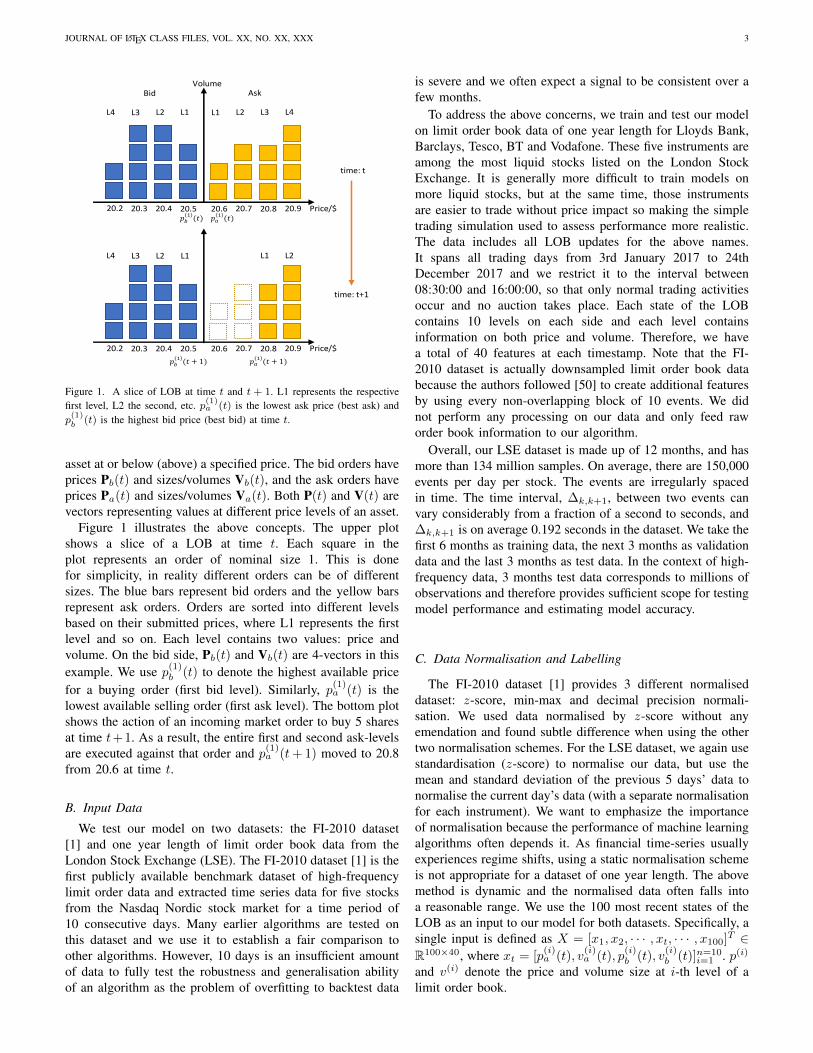
Figure 1. A slice of LOB at time t and t + 1. L1 represents the respectivefirst level, L2 the second, etc. p(1)a (t) is the lowest ask price (best ask) andp(1)b (t) is the highest bid price (best bid) at time t.

asset at or below (above) a specified price. The bid orders haveprices Pb(t) and sizes/volumes Vb(t), and the ask orders haveprices Pa(t) and sizes/volumes Va(t). Both P(t) and V(t) arevectors representing values at different price levels of an asset.

Figure 1 illustrates the above concepts. The upper plotshows a slice of a LOB at time t. Each square in theplot represents an order of nominal size 1. This is donefor simplicity, in reality different orders can be of differentsizes. The blue bars represent bid orders and the yellow barsrepresent ask orders. Orders are sorted into different levelsbased on their submitted prices, where L1 represents the firstlevel and so on. Each level contains two values: price andvolume. On the bid side, Pb(t) and Vb(t) are 4-vectors in thisexample. We use p(1)b (t) to denote the highest available pricefor a buying order (first bid level). Similarly, p(1)a (t) is thelowest available selling order (first ask level). The bottom plotshows the action of an incoming market order to buy 5 sharesat time t+1. As a result, the entire first and second ask-levelsare executed against that order and p(1)a (t+ 1) moved to 20.8from 20.6 at time t.

B. Input Data

We test our model on two datasets: the FI-2010 dataset[1] and one year length of limit order book data from theLondon Stock Exchange (LSE). The FI-2010 dataset [1] is thefirst publicly available benchmark dataset of high-frequencylimit order data and extracted time series data for five stocksfrom the Nasdaq Nordic stock market for a time period of10 consecutive days. Many earlier algorithms are tested onthis dataset and we use it to establish a fair comparison toother algorithms. However, 10 days is an insufficient amountof data to fully test the robustness and generalisation abilityof an algorithm as the problem of overfitting to backtest data

is severe and we often expect a signal to be consistent over afew months.

To address the above concerns, we train and test our modelon limit order book data of one year length for Lloyds Bank,Barclays, Tesco, BT and Vodafone. These five instruments areamong the most liquid stocks listed on the London StockExchange. It is generally more difficult to train models onmore liquid stocks, but at the same time, those instrumentsare easier to trade without price impact so making the simpletrading simulation used to assess performance more realistic.The data includes all LOB updates for the above names.It spans all trading days from 3rd January 2017 to 24thDecember 2017 and we restrict it to the interval between08:30:00 and 16:00:00, so that only normal trading activitiesoccur and no auction takes place. Each state of the LOBcontains 10 levels on each side and each level containsinformation on both price and volume. Therefore, we havea total of 40 features at each timestamp. Note that the FI-2010 dataset is actually downsampled limit order book databecause the authors followed [50] to create additional featuresby using every non-overlapping block of 10 events. We didnot perform any processing on our data and only feed raworder book information to our algorithm.

Overall, our LSE dataset is made up of 12 months, and hasmore than 134 million samples. On average, there are 150,000events per day per stock. The events are irregularly spacedin time. The time interval, ∆k,k+1, between two events canvary considerably from a fraction of a second to seconds, and∆k,k+1 is on average 0.192 seconds in the dataset. We take thefirst 6 months as training data, the next 3 months as validationdata and the last 3 months as test data. In the context of high-frequency data, 3 months test data corresponds to millions ofobservations and therefore provides sufficient scope for testingmodel performance and estimating model accuracy.

C. Data Normalisation and Labelling

The FI-2010 dataset [1] provides 3 different normaliseddataset: z-score, min-max and decimal precision normali-sation. We used data normalised by z-score without anyemendation and found subtle difference when using the othertwo normalisation schemes. For the LSE dataset, we again usestandardisation (z-score) to normalise our data, but use themean and standard deviation of the previous 5 days’ data tonormalise the current day’s data (with a separate normalisationfor each instrument). We want to emphasize the importanceof normalisation because the performance of machine learningalgorithms often depends it. As financial time-series usuallyexperiences regime shifts, using a static normalisation schemeis not appropriate for a dataset of one year length. The abovemethod is dynamic and the normalised data often falls intoa reasonable range. We use the 100 most recent states of theLOB as an input to our model for both datasets. Specifically, asingle input is defined as X = [x1, x2, · · · , xt, · · · , x100]T ∈R100×40, where xt = [p

(i)a (t), v

(i)a (t), p

(i)b (t), v

(i)b (t)]n=10

i=1 . p(i)

and v(i) denote the price and volume size at i-th level of alimit order book.

JOURNAL OF LATEX CLASS FILES, VOL. XX, NO. XX, XXX 4

After normalising the limit order data, we use the mid-price

pt =p(1)a (t) + p

(1)b (t)

2, (1)

to create labels that represent the direction of price changes.Although no order can transact exactly at the mid-price,it expresses a general market value for an asset and it isfrequently quoted when we want a single number to representan asset price.

Because financial data is highly stochastic, if we simplycompare pt and pt+k to decide the price movement, theresulting label set will be noisy. In the works of [1] and [26],two smoothing labelling methods are introduced. We brieflyrecall the two methods here. First, let m− denote the meanof the previous k mid-prices and m+ denote the mean of thenext k mid-prices:

m−(t) =1

k

k∑i=0

pt−i

m+(t) =1

k

k∑i=1

pt+i

(2)

where pt is the mid-price defined in Equation (1) and k is theprediction horizon. Both methods use the percentage change(lt) of the mid-price to decide directions. We can now define

lt =m+(t)− pt

pt(3)

lt =m+(t)−m−(t)

m−(t)(4)

Both are methods to define the direction of price movementat time t, where the former, Equation 3, was used in [1] andthe latter, Equation 4, in [26].

The labels are then decided based on a threshold (α) forthe percentage change (lt). If lt > α or lt < −α, we defineit as up (+1) or down (−1). For anything else, we considerit as stationary (0). Figure 2 provides a graphical illustrationof two labelling methods on the same threshold (α) and thesame prediction horizon (k). All the labels classified as down(−1) are shown as red areas and up (+1) as green areas. Theuncoloured (white) regions correspond to stationary (0) labels.

The FI-2010 dataset [1] adopts the method in Equation 3and we directly used their labels for fair comparison to othermethods. However, the produced labels are less consistent asshown on the top of Figure 2 because this method fits closerto real prices as smoothing is only applied to future prices.This is essentially detrimental for designing trading algorithmsas signals are not consistent here leading to many redundanttrading actions thus incurring larger transaction costs.

Further, the FI-2010 dataset was collected in 2010 andthe instruments were less liquid compared to now. We ex-perimented with this approach in [1] on our data from theLondon Stock Exchange and found the resulting labels arerather stochastic, therefore we adopt the method in Equation 4for our LSE dataset to produce more consistent signals.

0 200 400 600 800 100026.1026.1526.2026.2526.30 pt

0 200 400 600 800 100026.1026.1526.2026.2526.30 pt

Figure 2. An example of two smoothed labelling methods based on a samethreshold (α) and same prediction horizon (k). Green shading represents a +1signal and red a -1. Top: [1]’s method and Bottom: [26]’s method.

IV. MODEL ARCHITECTURE

A. Overview

We here detail our network architecture, which comprisesthree main building blocks: standard convolutional layers, anInception Module and a LSTM layer, as shown in Figure 3.The main idea of using CNNs and Inception Modules is toautomate the process of feature extraction as it is often difficultin financial applications since financial data is notoriouslynoisy with a low signal-to-noise ratio. Technical indicatorssuch as MACD and the Relative Strength Index are included asinputs and preprocessing mechanisms such as principal com-ponent analysis (PCA) [51] are often used to transform rawinputs. However, none of these processes is trivial, they maketacit assumptions and further, it is questionable if financialdata can be well-described with parametric models with fixedparameters. In our work, we only require the history of LOBprices and sizes as inputs to our algorithm. Weights are learnedduring inference and features, learned from a large training set,are data-adaptive, removing the above constraints. A LSTMlayer is then used to capture additional time dependenciesamong the resulting features. We note that very short time-dependencies are already captured in the convolutional layerwhich takes “space-time images” of the LOB as inputs.

B. Details of Each Component

a) Convolutional Layer: Recent development of elec-tronic trading algorithms often submit and cancel vast numbersof limit orders over short periods of time as part of theirtrading strategies [52]. These actions often take place deepin a LOB and it is seen [7] that more than 90% of orders endin cancellation rather than matching, therefore practitionersconsider levels further away from best bid and ask levels tobe less useful in any LOB. In addition, the work of [53]suggests that the best ask and best bid (L1-Ask and L1-Bid)contribute most to the price discovery and the contributionof all other levels is considerably less, estimated at as littleas 20%. As a result, it would be otiose to feed all levelinformation to a neural network as levels deep in a LOB areless useful and can potentially even be misleading. Naturally,we can smooth these signals by summarising the informationcontained in deeper levels. We note that convolution filtersused in any CNN architecture are discrete convolutions, orfinite impulse response (FIR) filters, from the viewpoint of

JOURNAL OF LATEX CLASS FILES, VOL. XX, NO. XX, XXX 5

Input

Conv1x2@16 (1,2)

4x1@164x1@16

1x10@164x1@164x1@16

1x10@164x1@164x1@16

Conv1x10@164x1@164x1@16

Conv1x10@164x1@164x1@16

Inception@32

LSTM@64 Units

Conv1x2@16 (stride = 1x2)

4x1@164x1@16

1x2@16 (stride = 1x2)4x1@164x1@16

1x10@164x1@164x1@16

Figure 3. Model architecture schematic. Here 1x2@16 represents a convolu-tional layer with 16 filters of size (1× 2). ‘1’ convolves through time indicesand ‘2’ convolves different limit order book levels.

signal processing [54]. FIR filters are popular smoothingtechniques for denoising target signals and they are simpleto implement and work with. We can write any FIR filter inthe following form:

y(n) =

M∑k=0

bkx(n− k) (5)

where the output signal y(n) at any time is a weighted sumof a finite number of past values of the input signal x(n). Thefilter order is denoted as M and bk is the filter coefficient.In a convolutional neural network, the coefficients of thefilter kernel are not obtained via a statistical objective fromtraditional signal filtration theory, but are left as degrees offreedom which the network infers so as to extremise its valuefunction at output.

The details of the first convolutional layer inevitably needsome consideration. As convolutional layers operate a smallkernel to “scan” through input data, the layout of limit orderbook information is vital. Recall that we take the most 100recent updates of an order book to form a single input andthere are 40 features per time stamp, so the size of a singleinput is (100× 40). We organise the 40 features as following:

{p(i)a (t), v(i)a (t), p(i)b (t), v

(i)b (t)}n=10

i=1 (6)

where i denotes the i-th level of a limit order book. Thesize of our first convolutional filter is (1 × 2) with stride of(1 × 2). The first layer essentially summarises informationbetween price and volume {p(i), v(i)} at each order booklevel. The usage of stride is necessary here as an importantproperty of convolutional layers is parameter sharing. Thisproperty is attractive as less parameters are estimated, largelyavoiding overfitting problems. However, without strides, wewould apply same parameters to {p(i), v(i)} and {v(i), p(i+1)}.In other words, p(i) and v(i) would share same parameters

because the kernel filter moves by one step, which is obviouslywrong as price and volume form different dynamic behaviors.

Because the first layer only captures information at eachorder book level, we would expect representative features to beextracted when integrating information across multiple orderbook levels. We can do this by utilising another convolutionallayer with filter size (1× 2) and stride (1× 2). The resultingfeature maps actually form the micro-price defined by [55]:

pmicro price = Ip(1)a + (1− I)p(1)b

I =v(1)b

v(1)a + v

(1)b

(7)

The weight I is called the imbalance. The micro-price is animportant indicator as it considers volumes on bid and ask side,and the imbalance between bid and ask size is a very strongindicator of the next price move. This feature of imbalanceshas been reported by a variety of researchers [56, 57, 58, 59,60]. Unlike the micro-price where only the first order booklevel is considered, we utilise convolutions to form micro-prices for all levels of a LOB so the resulting features mapsare of size (100, 10) after two layers with strides. Finally, weintegrate all information by using a large filter of size (1×10)and the dimension of our feature maps before the InceptionModule is (100, 1).

We apply zero padding to every convolutional layer so thetime dimension of our inputs does not change and Leaky Rec-tifying Linear Units (Leaky-ReLU) [61] are used as activationfunctions. The hyper-parameter (the small gradient when theunit is not active) of the Leaky-ReLU is set to 0.01, evaluatedby grid search on the validation set.

Another important property of convolution is that of equiv-ariance to translation [62]. Specifically, a function f(x) isequivariant to a function g if f(g(x)) = g(f(x)). For example,suppose that there exists a main classification feature mlocated at (xm, ym) of an image I(x, y). If we shift everypixel of I one unit to the right, we get a new image I ′

where I ′(x, y) = I(x − 1, y). We can still obtain the mainclassification feature m′ in I ′ and m = m′, while the locationof m′ will be at (xm′ , ym′) = (xm−1, ym). This is importantto time-series data, because convolution can find universalfeatures that are decisive to final outputs. In our case, supposea feature that studies imbalance is obtained at time t. If thesame event happens later at time t′ in the input, the exactfeature can be extracted later at t′.

We do not use any pooling layer except in the InceptionModules. Although pooling layers help us find representationsinvariant to translations of the input, the smoothing natureof pooling can cause under-fitting. Common pooling layersare designed for image processing tasks, and they are mostpowerful when we only care if certain features exist in theinputs instead of where they exist [62]. Time-series datahas different characteristics from images and the location ofrepresentative features is important. Our experiences showthat pooling layers in the convolutional layer, at least, causeunder-fitting problems to the LOB data. However, we thinkpooling is important and new pooling methods should bedesigned to process time-series data as it is a promising

JOURNAL OF LATEX CLASS FILES, VOL. XX, NO. XX, XXX 6

Input

1x1@16

25*1

1x1@16 1x1@16

100*40

50*1

3x40@16 10x40@16 20x40@16

Concat

1x1@16 1x1@16 1x1@16

3x1@16 10x1@16 20x1@16

Concat

Maxpool

1x1@16 1x1@16 1x1@16

3x1@16 10x1@16 20x1@16

Concat

1x1@16 1x1@16 1x1@16

3x1@16 10x1@16 20x1@16

Concat

Maxpool

12*1

1x1@16 1x1@16 1x1@16

3x1@16 10x1@16 20x1@16

Concat

1x1@16 1x1@16 1x1@16 3x1@16 10x1@16 20x1@16 Avgpool

3x1@32

5x1@32 1x1@32

Concat

Conv 1x1@32

Conv 3x1@32

Conv 1x1@32

Conv 5x1@32

Maxpool 3x1

Conv 1x1@32

Concat Inception@32

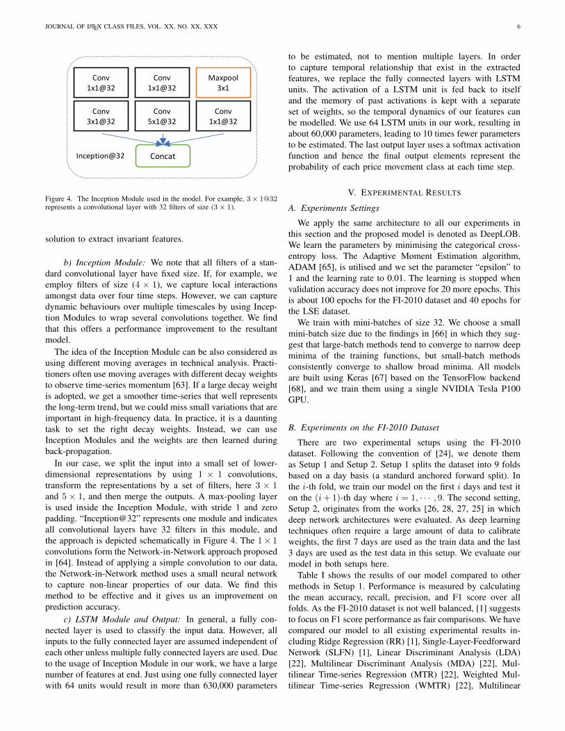
Figure 4. The Inception Module used in the model. For example, 3× 1@32represents a convolutional layer with 32 filters of size (3× 1).

solution to extract invariant features.

b) Inception Module: We note that all filters of a stan-dard convolutional layer have fixed size. If, for example, weemploy filters of size (4 × 1), we capture local interactionsamongst data over four time steps. However, we can capturedynamic behaviours over multiple timescales by using Incep-tion Modules to wrap several convolutions together. We findthat this offers a performance improvement to the resultantmodel.

The idea of the Inception Module can be also considered asusing different moving averages in technical analysis. Practi-tioners often use moving averages with different decay weightsto observe time-series momentum [63]. If a large decay weightis adopted, we get a smoother time-series that well representsthe long-term trend, but we could miss small variations that areimportant in high-frequency data. In practice, it is a dauntingtask to set the right decay weights. Instead, we can useInception Modules and the weights are then learned duringback-propagation.

In our case, we split the input into a small set of lower-dimensional representations by using 1 × 1 convolutions,transform the representations by a set of filters, here 3 × 1and 5 × 1, and then merge the outputs. A max-pooling layeris used inside the Inception Module, with stride 1 and zeropadding. “Inception@32” represents one module and indicatesall convolutional layers have 32 filters in this module, andthe approach is depicted schematically in Figure 4. The 1× 1convolutions form the Network-in-Network approach proposedin [64]. Instead of applying a simple convolution to our data,the Network-in-Network method uses a small neural networkto capture non-linear properties of our data. We find thismethod to be effective and it gives us an improvement onprediction accuracy.

c) LSTM Module and Output: In general, a fully con-nected layer is used to classify the input data. However, allinputs to the fully connected layer are assumed independent ofeach other unless multiple fully connected layers are used. Dueto the usage of Inception Module in our work, we have a largenumber of features at end. Just using one fully connected layerwith 64 units would result in more than 630,000 parameters

to be estimated, not to mention multiple layers. In orderto capture temporal relationship that exist in the extractedfeatures, we replace the fully connected layers with LSTMunits. The activation of a LSTM unit is fed back to itselfand the memory of past activations is kept with a separateset of weights, so the temporal dynamics of our features canbe modelled. We use 64 LSTM units in our work, resulting inabout 60,000 parameters, leading to 10 times fewer parametersto be estimated. The last output layer uses a softmax activationfunction and hence the final output elements represent theprobability of each price movement class at each time step.

V. EXPERIMENTAL RESULTS

A. Experiments Settings

We apply the same architecture to all our experiments inthis section and the proposed model is denoted as DeepLOB.We learn the parameters by minimising the categorical cross-entropy loss. The Adaptive Moment Estimation algorithm,ADAM [65], is utilised and we set the parameter “epsilon” to1 and the learning rate to 0.01. The learning is stopped whenvalidation accuracy does not improve for 20 more epochs. Thisis about 100 epochs for the FI-2010 dataset and 40 epochs forthe LSE dataset.

We train with mini-batches of size 32. We choose a smallmini-batch size due to the findings in [66] in which they sug-gest that large-batch methods tend to converge to narrow deepminima of the training functions, but small-batch methodsconsistently converge to shallow broad minima. All modelsare built using Keras [67] based on the TensorFlow backend[68], and we train them using a single NVIDIA Tesla P100GPU.

B. Experiments on the FI-2010 Dataset

There are two experimental setups using the FI-2010dataset. Following the convention of [24], we denote themas Setup 1 and Setup 2. Setup 1 splits the dataset into 9 foldsbased on a day basis (a standard anchored forward split). Inthe i-th fold, we train our model on the first i days and test iton the (i+ 1)-th day where i = 1, · · · , 9. The second setting,Setup 2, originates from the works [26, 28, 27, 25] in whichdeep network architectures were evaluated. As deep learningtechniques often require a large amount of data to calibrateweights, the first 7 days are used as the train data and the last3 days are used as the test data in this setup. We evaluate ourmodel in both setups here.

Table I shows the results of our model compared to othermethods in Setup 1. Performance is measured by calculatingthe mean accuracy, recall, precision, and F1 score over allfolds. As the FI-2010 dataset is not well balanced, [1] suggeststo focus on F1 score performance as fair comparisons. We havecompared our model to all existing experimental results in-cluding Ridge Regression (RR) [1], Single-Layer-FeedforwardNetwork (SLFN) [1], Linear Discriminant Analysis (LDA)[22], Multilinear Discriminant Analysis (MDA) [22], Mul-tilinear Time-series Regression (MTR) [22], Weighted Mul-tilinear Time-series Regression (WMTR) [22], Multilinear

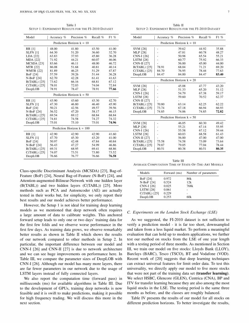
JOURNAL OF LATEX CLASS FILES, VOL. XX, NO. XX, XXX 7

Table ISETUP 1: EXPERIMENT RESULTS FOR THE FI-2010 DATASET

Model Accuracy % Precision % Recall % F1 %

Prediction Horizon k = 10

RR [1] 48.00 41.80 43.50 41.00SLFN [1] 64.30 51.20 36.60 32.70LDA [22] 63.83 37.93 45.80 36.28MDA [22] 71.92 44.21 60.07 46.06MCSDA [23] 83.66 46.11 48.00 46.72MTR [22] 86.08 51.68 40.81 40.14WMTR [22] 81.89 46.25 51.29 47.87BoF [24] 57.59 39.26 51.44 36.28N-BoF [24] 62.70 42.28 61.41 41.63B(TABL) [25] 73.62 66.16 68.81 67.12C(TABL) [25] 78.01 72.03 74.04 72.84DeepLOB 78.91 78.47 78.91 77.66

Prediction Horizon k = 50

RR [1] 43.90 43.60 43.30 42.70SLFN [1] 47.30 46.80 46.40 45.90BoF [24] 50.21 42.56 49.57 39.56N-BoF [24] 56.52 47.20 58.17 46.15B(TABL) [25] 69.54 69.12 68.84 68.84C(TABL) [25] 74.81 74.58 74.27 74.32DeepLOB 75.01 75.10 75.01 74.96

Prediction Horizon k = 100

RR [1] 42.90 42.90 42.90 41.60SLFN [1] 47.70 45.30 43.20 41.00BoF [24] 50.97 42.48 47.84 40.84N-BoF [24] 56.43 47.27 54.99 46.86B(TABL) [25] 69.31 68.95 69.41 68.86C(TABL) [25] 74.07 73.51 73.80 73.52DeepLOB 76.66 76.77 76.66 76.58

Class-specific Discriminant Analysis (MCSDA) [23], Bag-of-Feature (BoF) [24], Neural Bag-of-Feature (N-BoF) [24], andAttention-augmented-Bilinear-Network with one hidden layer(B(TABL)) and two hidden layers (C(TABL)) [25]. Moremethods such as PCA and Autoencoder (AE) are actuallytested in their works but, for simplicity, we only report theirbest results and our model achieves better performance.

However, the Setup 1 is not ideal for training deep learningmodels as we mentioned that deep network often requiresa large amount of data to calibrate weights. This anchoredforward setup leads to only one or two days’ training data forthe first few folds and we observe worse performance in thefirst few days. As training data grows, we observe remarkablybetter results as shown in Table II which shows the resultsof our network compared to other methods in Setup 2. Inparticular, the important difference between our model andCNN-I [26] and CNN-II [27] is due to network architectureand we can see huge improvements on performance here. InTable III, we compare the parameter sizes of DeepLOB withCNN-I [26]. Although our model has many more layers, thereare far fewer parameters in our network due to the usage ofLSTM layers instead of fully connected layers.

We also report the computation time (forward pass) inmilliseconds (ms) for available algorithms in Table III. Dueto the development of GPUs, training deep networks is nowfeasible and it is swift to make predictions, making it possiblefor high frequency trading. We will discuss this more in thenext section.

Table IISETUP 2: EXPERIMENT RESULTS FOR THE FI-2010 DATASET

Model Accuracy % Precision % Recall % F1 %

Prediction Horizon k = 10

SVM [28] - 39.62 44.92 35.88MLP [28] - 47.81 60.78 48.27CNN-I [26] - 50.98 65.54 55.21LSTM [28] - 60.77 75.92 66.33CNN-II [27] - 56.00 45.00 44.00B(TABL) [25] 78.91 68.04 71.21 69.20C(TABL) [25] 84.70 76.95 78.44 77.63DeepLOB 84.47 84.00 84.47 83.40

Prediction Horizon k = 20

SVM [28] - 45.08 47.77 43.20MLP [28] - 51.33 65.20 51.12CNN-I [26] - 54.79 67.38 59.17LSTM [28] - 59.60 70.52 62.37CNN-II [27] - - - -B(TABL) [25] 70.80 63.14 62.25 62.22C(TABL) [25] 73.74 67.18 66.94 66.93DeepLOB 74.85 74.06 74.85 72.82

Prediction Horizon k = 50

SVM [28] - 46.05 60.30 49.42MLP [28] - 55.21 67.14 55.95CNN-I [26] - 55.58 67.12 59.44LSTM [28] - 60.03 68.58 61.43CNN-II [27] - 56.00 47.00 47.00B(TABL) [25] 75.58 74.58 73.09 73.64C(TABL) [25] 79.87 79.05 77.04 78.44DeepLOB 80.51 80.38 80.51 80.35

Table IIIAVERAGE COMPUTATION TIME OF STATE-OF-THE-ART MODELS

Models Forward (ms) Number of parameters

BoF [24] 0.972 86kN-BoF [24] 0.524 12kCNN-I [26] 0.025 768kLSTM [28] 0.061 -C(TABL) [25] 0.229 -DeepLOB 0.253 60k

C. Experiments on the London Stock Exchange (LSE)

As we suggested, the FI-2010 dataset is not sufficient toverify a prediction model - it is far too short, downsampledand taken from a less liquid market. To perform a meaningfulevaluation that can hold up to modern applications, we furthertest our method on stocks from the LSE of one year lengthwith a testing period of three months. As mentioned in SectionIII, we train our model on five stocks: Lloyds Bank (LLOY),Barclays (BARC), Tesco (TSCO), BT and Vodafone (VOD).Recent work of [20] suggests that deep learning techniquescan extract universal features for limit order data. To test thisuniversality, we directly apply our model to five more stocksthat were not part of the training data set (transfer learning).We select HSBC, Glencore (GLEN), Centrica (CNA), BP andITV for transfer learning because they are also among the mostliquid stocks in the LSE. The testing period is the same threemonths as before, and the classes are roughly balanced.

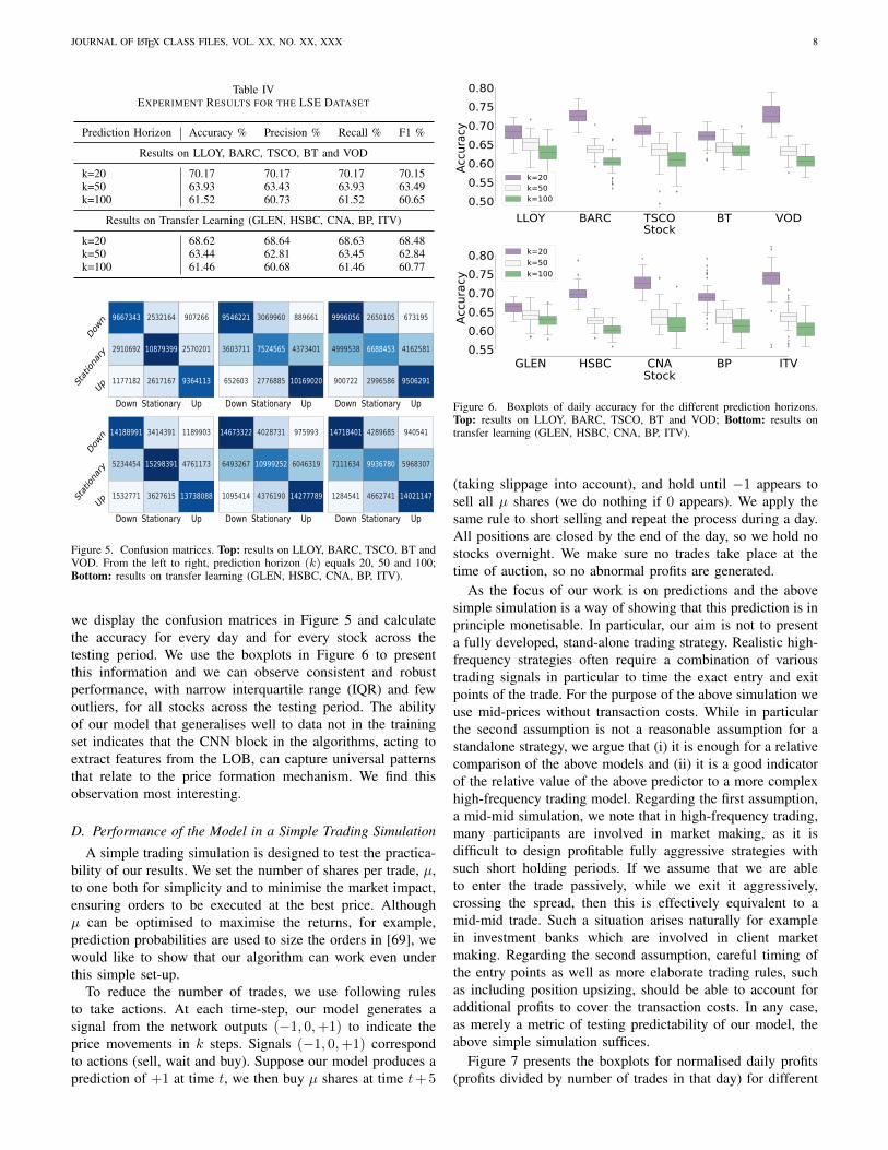
Table IV presents the results of our model for all stocks ondifferent prediction horizons. To better investigate the results,

JOURNAL OF LATEX CLASS FILES, VOL. XX, NO. XX, XXX 8

Table IVEXPERIMENT RESULTS FOR THE LSE DATASET

Prediction Horizon Accuracy % Precision % Recall % F1 %

Results on LLOY, BARC, TSCO, BT and VOD

k=20 70.17 70.17 70.17 70.15k=50 63.93 63.43 63.93 63.49k=100 61.52 60.73 61.52 60.65

Results on Transfer Learning (GLEN, HSBC, CNA, BP, ITV)

k=20 68.62 68.64 68.63 68.48k=50 63.44 62.81 63.45 62.84k=100 61.46 60.68 61.46 60.77

Down Stationary Up

Down

Statio

nary

Up

9667343 2532164 907266

2910692 10879399 2570201

1177182 2617167 9364113

Down Stationary Up

9546221 3069960 889661

3603711 7524565 4373401

652603 2776885 10169020

Down Stationary Up

9996056 2650105 673195

4999538 6688453 4162581

900722 2996586 9506291

Down Stationary Up

Down

Statio

nary

Up

14188991 3414391 1189903

5234454 15298391 4761173

1532771 3627615 13738088

Down Stationary Up

14673322 4028731 975993

6493267 10999252 6046319

1095414 4376190 14277789

Down Stationary Up

14718401 4289685 940541

7111634 9936780 5968307

1284541 4662741 14021147

Figure 5. Confusion matrices. Top: results on LLOY, BARC, TSCO, BT andVOD. From the left to right, prediction horizon (k) equals 20, 50 and 100;Bottom: results on transfer learning (GLEN, HSBC, CNA, BP, ITV).

we display the confusion matrices in Figure 5 and calculatethe accuracy for every day and for every stock across thetesting period. We use the boxplots in Figure 6 to presentthis information and we can observe consistent and robustperformance, with narrow interquartile range (IQR) and fewoutliers, for all stocks across the testing period. The abilityof our model that generalises well to data not in the trainingset indicates that the CNN block in the algorithms, acting toextract features from the LOB, can capture universal patternsthat relate to the price formation mechanism. We find thisobservation most interesting.

D. Performance of the Model in a Simple Trading Simulation

A simple trading simulation is designed to test the practica-bility of our results. We set the number of shares per trade, µ,to one both for simplicity and to minimise the market impact,ensuring orders to be executed at the best price. Althoughµ can be optimised to maximise the returns, for example,prediction probabilities are used to size the orders in [69], wewould like to show that our algorithm can work even underthis simple set-up.

To reduce the number of trades, we use following rulesto take actions. At each time-step, our model generates asignal from the network outputs (−1, 0,+1) to indicate theprice movements in k steps. Signals (−1, 0,+1) correspondto actions (sell, wait and buy). Suppose our model produces aprediction of +1 at time t, we then buy µ shares at time t+ 5

LLOY BARC TSCO BT VODStock

0.500.550.600.650.700.750.80

Accu

racy

k=20k=50k=100

GLEN HSBC CNA BP ITVStock

0.550.600.650.700.750.80

Accu

racy

k=20k=50k=100

Figure 6. Boxplots of daily accuracy for the different prediction horizons.Top: results on LLOY, BARC, TSCO, BT and VOD; Bottom: results ontransfer learning (GLEN, HSBC, CNA, BP, ITV).

(taking slippage into account), and hold until −1 appears tosell all µ shares (we do nothing if 0 appears). We apply thesame rule to short selling and repeat the process during a day.All positions are closed by the end of the day, so we hold nostocks overnight. We make sure no trades take place at thetime of auction, so no abnormal profits are generated.

As the focus of our work is on predictions and the abovesimple simulation is a way of showing that this prediction is inprinciple monetisable. In particular, our aim is not to presenta fully developed, stand-alone trading strategy. Realistic high-frequency strategies often require a combination of varioustrading signals in particular to time the exact entry and exitpoints of the trade. For the purpose of the above simulation weuse mid-prices without transaction costs. While in particularthe second assumption is not a reasonable assumption for astandalone strategy, we argue that (i) it is enough for a relativecomparison of the above models and (ii) it is a good indicatorof the relative value of the above predictor to a more complexhigh-frequency trading model. Regarding the first assumption,a mid-mid simulation, we note that in high-frequency trading,many participants are involved in market making, as it isdifficult to design profitable fully aggressive strategies withsuch short holding periods. If we assume that we are ableto enter the trade passively, while we exit it aggressively,crossing the spread, then this is effectively equivalent to amid-mid trade. Such a situation arises naturally for examplein investment banks which are involved in client marketmaking. Regarding the second assumption, careful timing ofthe entry points as well as more elaborate trading rules, suchas including position upsizing, should be able to account foradditional profits to cover the transaction costs. In any case,as merely a metric of testing predictability of our model, theabove simple simulation suffices.

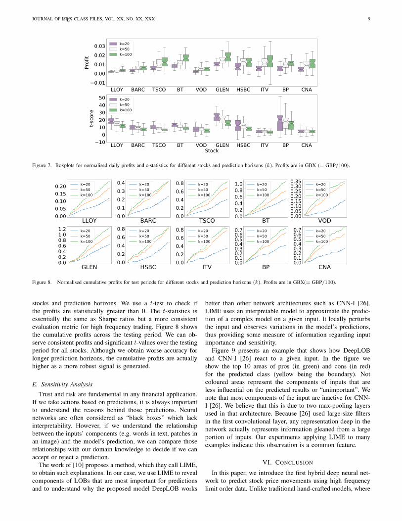
Figure 7 presents the boxplots for normalised daily profits(profits divided by number of trades in that day) for different

JOURNAL OF LATEX CLASS FILES, VOL. XX, NO. XX, XXX 9

LLOY BARC TSCO BT VOD GLEN HSBC ITV BP CNA0.010.000.010.020.03

Prof

it

k=20k=50k=100

LLOY BARC TSCO BT VOD GLEN HSBC ITV BP CNAStock

100

1020304050

t-sco

rek=20k=50k=100

Figure 7. Boxplots for normalised daily profits and t-statistics for different stocks and prediction horizons (k). Profits are in GBX (= GBP/100).

LLOY0.000.050.100.150.20 k=20

k=50k=100

BARC0.00.10.20.30.4 k=20

k=50k=100

TSCO0.00.20.40.60.8 k=20

k=50k=100

BT0.00.20.40.60.81.0 k=20

k=50k=100

VOD0.000.050.100.150.200.250.300.35 k=20

k=50k=100

GLEN0.00.20.40.60.81.01.2 k=20

k=50k=100

HSBC0.00.20.40.60.8 k=20

k=50k=100

ITV0.00.20.40.60.8 k=20

k=50k=100

BP0.00.10.20.30.40.50.60.7 k=20

k=50k=100

CNA0.00.10.20.30.40.50.60.7 k=20

k=50k=100

Figure 8. Normalised cumulative profits for test periods for different stocks and prediction horizons (k). Profits are in GBX(= GBP/100).

stocks and prediction horizons. We use a t-test to check ifthe profits are statistically greater than 0. The t-statistics isessentially the same as Sharpe ratios but a more consistentevaluation metric for high frequency trading. Figure 8 showsthe cumulative profits across the testing period. We can ob-serve consistent profits and significant t-values over the testingperiod for all stocks. Although we obtain worse accuracy forlonger prediction horizons, the cumulative profits are actuallyhigher as a more robust signal is generated.

E. Sensitivity Analysis

Trust and risk are fundamental in any financial application.If we take actions based on predictions, it is always importantto understand the reasons behind those predictions. Neuralnetworks are often considered as “black boxes” which lackinterpretability. However, if we understand the relationshipbetween the inputs’ components (e.g. words in text, patches inan image) and the model’s prediction, we can compare thoserelationships with our domain knowledge to decide if we canaccept or reject a prediction.

The work of [10] proposes a method, which they call LIME,to obtain such explanations. In our case, we use LIME to revealcomponents of LOBs that are most important for predictionsand to understand why the proposed model DeepLOB works

better than other network architectures such as CNN-I [26].LIME uses an interpretable model to approximate the predic-tion of a complex model on a given input. It locally perturbsthe input and observes variations in the model’s predictions,thus providing some measure of information regarding inputimportance and sensitivity.

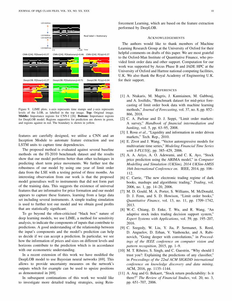
Figure 9 presents an example that shows how DeepLOBand CNN-I [26] react to a given input. In the figure weshow the top 10 areas of pros (in green) and cons (in red)for the predicted class (yellow being the boundary). Notcoloured areas represent the components of inputs that areless influential on the predicted results or “unimportant”. Wenote that most components of the input are inactive for CNN-I [26]. We believe that this is due to two max-pooling layersused in that architecture. Because [26] used large-size filtersin the first convolutional layer, any representation deep in thenetwork actually represents information gleaned from a largeportion of inputs. Our experiments applying LIME to manyexamples indicate this observation is a common feature.

VI. CONCLUSION

In this paper, we introduce the first hybrid deep neural net-work to predict stock price movements using high frequencylimit order data. Unlike traditional hand-crafted models, where

JOURNAL OF LATEX CLASS FILES, VOL. XX, NO. XX, XXX 10

Real label = Stationary

Ref: P(Down) = 0.27 Ref: P(Stationary) = 0.46 Ref: P(Up) = 0.27

DeepLOB: P(Down) = 0.27 DeepLOB: P(Stationary) = 0.71 DeepLOB: P(Up) = 0.04

L10-AskSize

L10-BidSize L10-AskPrice

L10-BidPrice

t=1 t=100 Time

CNN-I[24]: P(Down)=0.27 CNN-I[24]: P(Stationary)=0.46 CNN-I[24]: P(Up)=0.27

DeepLOB: P(Up)=0.04DeepLOB: P(Stationary)=0.71DeepLOB: P(Down)=0.27

Figure 9. LIME plots. x-axis represents time stamps and y-axis representslevels of the LOB, as labelled in the top image. Top: Original image.Middle: Importance regions for CNN-I [26]. Bottom: Importance regionsfor DeepLOB model. Regions supportive for prediction are shown in green,and regions against in red. The boundary is shown in yellow.

features are carefully designed, we utilise a CNN and anInception Module to automate feature extraction and useLSTM units to capture time dependencies.

The proposed method is evaluated against several baselinemethods on the FI-2010 benchmark dataset and the resultsshow that our model performs better than other techniques inpredicting short term price movements. We further test therobustness of our model by using one year of limit orderdata from the LSE with a testing period of three months. Aninteresting observation from our work is that the proposedmodel generalises well to instruments that did not form partof the training data. This suggests the existence of universalfeatures that are informative for price formation and our modelappears to capture these features, learning from a large dataset including several instruments. A simple trading simulationis used to further test our model and we obtain good profitsthat are statistically significant.

To go beyond the often-criticised “black box” nature ofdeep learning models, we use LIME, a method for sensitivityanalysis, to indicate the components of inputs that contribute topredictions. A good understanding of the relationship betweenthe input’s components and the model’s prediction can helpus decide if we can accept a prediction. In particular, we seehow the information of prices and sizes on different levels andhorizons contribute to the prediction which is in accordancewith our econometric understanding.

In a recent extension of this work we have modified theDeepLOB model to use Bayesian neural networks [69]. Thisallows to provide uncertainty measures on the network’soutputs which for example can be used to upsize positionsas demonstrated in [69].

In subsequent continuations of this work we would liketo investigate more detailed trading strategies, using Rein-

forcement Learning, which are based on the feature extractionperformed by DeepLOB.

ACKNOWLEDGEMENTS

The authors would like to thank members of MachineLearning Research Group at the University of Oxford for theirhelpful comments on drafts of this paper. We are most gratefulto the Oxford-Man Institute of Quantitative Finance, who pro-vided limit order data and other support. Computation for ourwork was supported by Arcus Phase B and JADE HPC at theUniversity of Oxford and Hartree national computing facilities,U.K. We also thank the Royal Academy of Engineering U.K.for their support.

REFERENCES

[1] A. Ntakaris, M. Magris, J. Kanniainen, M. Gabbouj,and A. Iosifidis, “Benchmark dataset for mid-price fore-casting of limit order book data with machine learningmethods,” Journal of Forecasting, vol. 37, no. 8, pp. 852–866, 2018.

[2] C. A. Parlour and D. J. Seppi, “Limit order markets:A survey,” Handbook of financial intermediation andbanking, vol. 5, pp. 63–95, 2008.

[3] I. Rosu et al., “Liquidity and information in order drivenmarkets,” Tech. Rep., 2010.

[4] E. Zivot and J. Wang, “Vector autoregressive models formultivariate time series,” Modeling Financial Time Serieswith S-PLUS R©, pp. 385–429, 2006.

[5] A. A. Ariyo, A. O. Adewumi, and C. K. Ayo, “Stockprice prediction using the ARIMA model,” in ComputerModelling and Simulation (UKSim), 2014 UKSim-AMSS16th International Conference on. IEEE, 2014, pp. 106–112.

[6] C. Carrie, “The new electronic trading regime of darkbooks, mashups and algorithmic trading,” Trading, vol.2006, no. 1, pp. 14–20, 2006.

[7] M. D. Gould, M. A. Porter, S. Williams, M. McDonald,D. J. Fenn, and S. D. Howison, “Limit order books,”Quantitative Finance, vol. 13, no. 11, pp. 1709–1742,2013.

[8] W.-C. Chiang, D. Enke, T. Wu, and R. Wang, “Anadaptive stock index trading decision support system,”Expert Systems with Applications, vol. 59, pp. 195–207,2016.

[9] C. Szegedy, W. Liu, Y. Jia, P. Sermanet, S. Reed,D. Anguelov, D. Erhan, V. Vanhoucke, and A. Rabi-novich, “Going deeper with convolutions,” in Proceed-ings of the IEEE conference on computer vision andpattern recognition, 2015, pp. 1–9.

[10] M. T. Ribeiro, S. Singh, and C. Guestrin, “Why should Itrust you?: Explaining the predictions of any classifier,”in Proceedings of the 22nd ACM SIGKDD internationalconference on knowledge discovery and data mining.ACM, 2016, pp. 1135–1144.

[11] A. Ang and G. Bekaert, “Stock return predictability: Is itthere?” The Review of Financial Studies, vol. 20, no. 3,pp. 651–707, 2006.

JOURNAL OF LATEX CLASS FILES, VOL. XX, NO. XX, XXX 11

[12] P. Bacchetta, E. Mertens, and E. Van Wincoop, “Pre-dictability in financial markets: What do survey expec-tations tell us?” Journal of International Money andFinance, vol. 28, no. 3, pp. 406–426, 2009.

[13] T. Bollerslev, J. Marrone, L. Xu, and H. Zhou, “Stockreturn predictability and variance risk premia: Statisticalinference and international evidence,” Journal of Finan-cial and Quantitative Analysis, vol. 49, no. 3, pp. 633–661, 2014.

[14] M. A. Ferreira and P. Santa-Clara, “Forecasting stockmarket returns: The sum of the parts is more than thewhole,” Journal of Financial Economics, vol. 100, no. 3,pp. 514–537, 2011.

[15] B. Mandelbrot and R. L. Hudson, The Misbehavior ofMarkets: A fractal view of financial turbulence. Basicbooks, 2007.

[16] B. B. Mandelbrot, “How Fractals Can Explain What’sWrong with Wall Street,” Scientific American, vol. 15,no. 9, p. 2008, 2008.

[17] J. Agrawal, V. Chourasia, and A. Mittra, “State-of-the-art in stock prediction techniques,” International Journalof Advanced Research in Electrical, Electronics andInstrumentation Engineering, vol. 2, no. 4, pp. 1360–1366, 2013.

[18] R. C. Cavalcante, R. C. Brasileiro, V. L. Souza, J. P.Nobrega, and A. L. Oliveira, “Computational intelligenceand financial markets: A survey and future directions,”Expert Systems with Applications, vol. 55, pp. 194–211,2016.

[19] Q. Cao, K. B. Leggio, and M. J. Schniederjans, “A com-parison between Fama and French’s model and artificialneural networks in predicting the Chinese stock market,”Computers Operations Research, vol. 32, no. 10, pp.2499–2512, 2005.

[20] J. Sirignano and R. Cont, “Universal features of priceformation in financial markets: perspectives from deeplearning,” arXiv preprint arXiv:1803.06917, 2018.

[21] G. S. Atsalakis and K. P. Valavanis, “Surveying stockmarket forecasting techniques–Part II: Soft computingmethods,” Expert Systems with Applications, vol. 36,no. 3, pp. 5932–5941, 2009.

[22] D. T. Tran, M. Magris, J. Kanniainen, M. Gabbouj,and A. Iosifidis, “Tensor representation in high-frequencyfinancial data for price change prediction,” in Computa-tional Intelligence (SSCI), 2017 IEEE Symposium Serieson. IEEE, 2017, pp. 1–7.

[23] D. T. Tran, M. Gabbouj, and A. Iosifidis, “Multilinearclass-specific discriminant analysis,” Pattern RecognitionLetters, vol. 100, pp. 131–136, 2017.

[24] N. Passalis, A. Tefas, J. Kanniainen, M. Gabbouj, andA. Iosifidis, “Temporal bag-of-features learning for pre-dicting mid price movements using high frequency limitorder book data,” IEEE Transactions on Emerging Topicsin Computational Intelligence, 2018.

[25] D. T. Tran, A. Iosifidis, J. Kanniainen, and M. Gabbouj,“Temporal attention-augmented bilinear network for fi-nancial time-series data analysis,” IEEE transactions onneural networks and learning systems, 2018.

[26] A. Tsantekidis, N. Passalis, A. Tefas, J. Kanniainen,M. Gabbouj, and A. Iosifidis, “Forecasting stock pricesfrom the limit order book using convolutional neuralnetworks,” in Business Informatics (CBI), 2017 IEEE19th Conference on, vol. 1. IEEE, 2017, pp. 7–12.

[27] ——, “Using Deep Learning for price prediction byexploiting stationary limit order book features,” arXivpreprint arXiv:1810.09965, 2018.

[28] ——, “Using deep learning to detect price change in-dications in financial markets,” in Signal ProcessingConference (EUSIPCO), 2017 25th European. IEEE,2017, pp. 2511–2515.

[29] M. Dixon, D. Klabjan, and J. H. Bang, “Classification-based financial markets prediction using deep neuralnetworks,” Algorithmic Finance, vol. 6, no. 3-4, pp. 67–77, 2017.

[30] Y. LeCun, Y. Bengio et al., “Convolutional networks forimages, speech, and time series,” The handbook of braintheory and neural networks, vol. 3361, no. 10, p. 1995,1995.

[31] N. Wang and D.-Y. Yeung, “Learning a deep compactimage representation for visual tracking,” in Advances inneural information processing systems, 2013, pp. 809–817.

[32] R. Girshick, J. Donahue, T. Darrell, and J. Malik, “Richfeature hierarchies for accurate object detection andsemantic segmentation,” in Proceedings of the IEEEconference on computer vision and pattern recognition,2014, pp. 580–587.

[33] J. Long, E. Shelhamer, and T. Darrell, “Fully convolu-tional networks for semantic segmentation,” in Proceed-ings of the IEEE Conference on Computer Vision andPattern Recognition, 2015, pp. 3431–3440.

[34] J.-F. Chen, W.-L. Chen, C.-P. Huang, S.-H. Huang, andA.-P. Chen, “Financial time-series data analysis usingdeep convolutional neural networks,” in Cloud Com-puting and Big Data (CCBD), 2016 7th InternationalConference on. IEEE, 2016, pp. 87–92.

[35] J. Doering, M. Fairbank, and S. Markose, “Convolu-tional neural networks applied to high-frequency marketmicrostructure forecasting,” in Computer Science andElectronic Engineering (CEEC), 2017. IEEE, 2017, pp.31–36.

[36] A. Krizhevsky, I. Sutskever, and G. E. Hinton, “Imagenetclassification with deep convolutional neural networks,”in Advances in neural information processing systems,2012, pp. 1097–1105.

[37] K. Simonyan and A. Zisserman, “Very Deep Convolu-tional Networks for Large-Scale Image Recognition,” inInternational Conference on Learning Representations,2015.

[38] S. Hochreiter and J. Schmidhuber, “Long short-termmemory,” Neural computation, vol. 9, no. 8, pp. 1735–1780, 1997.

[39] Y. Bengio, P. Simard, and P. Frasconi, “Learning long-term dependencies with gradient descent is difficult,”IEEE transactions on neural networks, vol. 5, no. 2, pp.157–166, 1994.

JOURNAL OF LATEX CLASS FILES, VOL. XX, NO. XX, XXX 12

[40] M. Sundermeyer, R. Schluter, and H. Ney, “LSTM neuralnetworks for language modeling,” in Thirteenth AnnualConference of the International Speech CommunicationAssociation, 2012.

[41] I. Sutskever, O. Vinyals, and Q. V. Le, “Sequence tosequence learning with neural networks,” in Advances inneural information processing systems, 2014, pp. 3104–3112.

[42] W. Bao, J. Yue, and Y. Rao, “A deep learning frameworkfor financial time series using stacked autoencoders andlong-short term memory,” PloS one, vol. 12, no. 7, p.e0180944, 2017.

[43] S. Selvin, R. Vinayakumar, E. Gopalakrishnan, V. K.Menon, and K. Soman, “Stock price prediction usingLSTM, RNN and CNN-sliding window model,” in Ad-vances in Computing, Communications and Informatics(ICACCI), 2017 International Conference on. IEEE,2017, pp. 1643–1647.

[44] T. Fischer and C. Krauss, “Deep learning with long short-term memory networks for financial market predictions,”European Journal of Operational Research, vol. 270,no. 2, pp. 654–669, 2018.

[45] L. Di Persio and O. Honchar, “Artificial neural networksarchitectures for stock price prediction: Comparisons andapplications,” International Journal of Circuits, Systemsand Signal Processing, vol. 10, pp. 403–413, 2016.

[46] M. Dixon, “Sequence classification of the limit orderbook using recurrent neural networks,” Journal of com-putational science, vol. 24, pp. 277–286, 2018.

[47] D. M. Nelson, A. C. Pereira, and R. A. de Oliveira,“Stock market’s price movement prediction with LSTMneural networks,” in Neural Networks (IJCNN), 2017International Joint Conference on. IEEE, 2017, pp.1419–1426.

[48] L. Harris, Trading and exchanges: Market microstructurefor practitioners. Oxford University Press, USA, 2003.

[49] M. O’Hara, Market microstructure theory. BlackwellPublishers Cambridge, MA, 1995, vol. 108.

[50] A. N. Kercheval and Y. Zhang, “Modelling high-frequency limit order book dynamics with Support VectorMachines,” Quantitative Finance, vol. 15, no. 8, pp.1315–1329, 2015.

[51] A. Abraham, B. Nath, and P. K. Mahanti, “Hybrid intelli-gent systems for stock market analysis,” in InternationalConference on Computational Science. Springer, 2001,pp. 337–345.

[52] T. Hendershott, C. M. Jones, and A. J. Menkveld, “Doesalgorithmic trading improve liquidity?” The Journal ofFinance, vol. 66, no. 1, pp. 1–33, 2011.

[53] C. Cao, O. Hansch, and X. Wang, “The informationcontent of an open limit-order book,” Journal of futuresmarkets, vol. 29, no. 1, pp. 16–41, 2009.

[54] S. J. Orfanidis, Introduction to signal processing.Prentice-Hall, Inc., 1995.

[55] J. Gatheral and R. C. Oomen, “Zero-intelligence realizedvariance estimation,” Finance and Stochastics, vol. 14,no. 2, pp. 249–283, 2010.

[56] Y. Nevmyvaka, Y. Feng, and M. Kearns, “Reinforcement

learning for optimized trade execution,” in Proceedingsof the 23rd international conference on Machine learn-ing. ACM, 2006, pp. 673–680.

[57] M. Avellaneda, J. Reed, and S. Stoikov, “Forecastingprices from Level-I quotes in the presence of hiddenliquidity,” Algorithmic Finance, vol. 1, no. 1, pp. 35–43,2011.

[58] Y. Burlakov, M. Kamal, and M. Salvadore, “Optimallimit order execution in a simple model for marketmicrostructure dynamics,” 2012.

[59] L. Harris, “Maker-taker pricing effects on market quo-tations,” USC Marshall School of Business Work-ing Paper. Avalable at http://bschool. huji. ac. il/.upload/hujibusiness/Maker-taker. pdf, 2013.

[60] A. Lipton, U. Pesavento, and M. G. Sotiropoulos, “Tradearrival dynamics and quote imbalance in a limit orderbook,” arXiv preprint arXiv:1312.0514, 2013.

[61] A. L. Maas, A. Y. Hannun, and A. Y. Ng, “Rectifiernonlinearities improve neural network acoustic models,”in Proc. icml, vol. 30, no. 1, 2013, p. 3.

[62] I. Goodfellow, Y. Bengio, and A. Courville, Deep Learn-ing. MIT Press, 2016,http://www.deeplearningbook.org.

[63] T. J. Moskowitz, Y. H. Ooi, and L. H. Pedersen, “Timeseries momentum,” Journal of financial economics, vol.104, no. 2, pp. 228–250, 2012.

[64] M. Lin, Q. Chen, and S. Yan, “Network in network,” inInternational Conference on Learning Representations,2014.

[65] D. Kingma and J. Ba, “Adam: A method for stochasticoptimization,” Proceedings of the International Confer-ence on Learning Representations 2015, 2015.

[66] N. S. Keskar, D. Mudigere, J. Nocedal, M. Smelyanskiy,and P. T. P. Tang, “On large-batch training for deeplearning: Generalization gap and sharp minima,” in Inter-national Conference on Learning Representations, 2017.

[67] F. Chollet et al., “Keras,” https://keras.io, 2015.[68] M. Abadi, A. Agarwal, P. Barham, E. Brevdo, Z. Chen,

C. Citro, G. S. Corrado, A. Davis, J. Dean, M. Devin,S. Ghemawat, I. Goodfellow, A. Harp, G. Irving,M. Isard, Y. Jia, R. Jozefowicz, L. Kaiser, M. Kudlur,J. Levenberg, D. Mane, R. Monga, S. Moore, D. Murray,C. Olah, M. Schuster, J. Shlens, B. Steiner, I. Sutskever,K. Talwar, P. Tucker, V. Vanhoucke, V. Vasudevan,F. Viegas, O. Vinyals, P. Warden, M. Wattenberg,M. Wicke, Y. Yu, and X. Zheng, “TensorFlow: Large-scale machine learning on heterogeneous systems,”2015, software available from tensorflow.org. [Online].Available: https://www.tensorflow.org/

[69] Z. Zhang, S. Zohren, and S. Roberts, “BDLOB: BayesianDeep Convolutional Neural Networks for Limit OrderBooks,” in Third workshop on Bayesian Deep Learning(NeurIPS 2018), 2018.