1

Graph Drawing by Stochastic Gradient DescentJonathan X. Zheng, Samraat Pawar, Dan F. M. Goodman

Abstract—A popular method of force-directed graph drawing is multidimensional scaling using graph-theoretic distances as input. Wepresent an algorithm to minimize its energy function, known as stress, by using stochastic gradient descent (SGD) to move a singlepair of vertices at a time. Our results show that SGD can reach lower stress levels faster and more consistently than majorization,without needing help from a good initialization. We then show how the unique properties of SGD make it easier to produce constrainedlayouts than previous approaches. We also show how SGD can be directly applied within the sparse stress approximation of Ortmannet al. [1], making the algorithm scalable up to large graphs.

Index Terms—Graph drawing, multidimensional scaling, constraints, relaxation, stochastic gradient descent

F

1 INTRODUCTION

G RAPHS are a common data structure, used to describeeverything from social networks to food webs, from

metabolic pathways to internet traffic. Any set of pairwiserelationships between entities can be described by a graph,and the ever increasing amount of data being collectedmeans that visualizing graphs for exploratory analysis hasbecome an important task.

Node-link diagrams are an intuitive representation ofgraphs, where vertices are represented by dots, and edgesby lines connecting them. A primary task is then to findsuitable coordinates for these dots that represent the datafaithfully. However this is far from trivial, and the difficultybehind finding a good layout can be illustrated through asimple example. If we consider the problem of drawinga tetrahedron in 2D space, it is easy to see that no ideallayout exists where all edges have equal lengths. Even forsuch a small graph with only four vertices, there are toofew dimensions available to provide sufficient degrees offreedom. The next logical question is: what layout gets asclose as possible to this ideal?

Multidimensional scaling (MDS) is a technique to solveexactly this type of problem, that attempts to minimizethe disparity between ideal and low-dimensional distances.This is done by defining an equation to quantify the error ina layout, and then minimizing it. While this equation comesin many forms [2], distance scaling is most commonly usedfor graphs [3], where the error is defined as

stress(X) =∑i<j

wij(||Xi −Xj || − dij)2 (1)

where X contains the coordinates of each vertex in low-dimensional space, and d is the ideal distance betweenthem. A weighting factor w is used to either emphasize ordampen the importance of certain pairs. For the problemof graph layout, the most common approach is to set dij

• Jonathan Zheng is with Department of Electrical and Electronic Engineer-ing, Imperial College London.E-mail: jxz12@ic.ac.uk

• Samraat Pawar is with Department of Life Sciences, Imperial CollegeLondon.

• Dan Goodman is with Department of Electrical and Electronic Engineer-ing, Imperial College London.

to the shortest path distance between vertices i and j, withwij = d−2ij to offset the extra weight given to longer pathsdue to squaring the difference [3].

This definition was popularized for graph layout byKamada and Kawai [4] who minimized the function usinga localized 2D Newton-Raphson method, while within theMDS community Kruskal [5] originally used gradient de-scent [6]. This was later improved upon by De Leeuw [7]with a method known as majorization, which minimizes acomplicated function by iteratively finding the true minimaof a series of simpler functions, each of which touches theoriginal function and is an upper bound for it [2]. This wasapplied to graph layout by Gansner et al. [8] and has beenthe state-of-the-art for the past decade. For larger graphs,fully computing stress is not feasible, and so we reviewapproximation methods in Section 4.3.

This paper describes a method of minimizing stress byusing stochastic gradient descent (SGD), which approxi-mates the gradient of a sum of functions using the gradientof its individual terms. In our case this corresponds to mov-ing a single pair of vertices at a time. The simplicity of eachterm in Equation (1) also allows for some modifications tothe step size which, combined with the added stochasticity,help to avoid local minima. We show the benefits of SGDover majorization through experiment.

The structure of this paper is as follows: the algorithmis described and its subtleties are explored; an experimentalstudy of its performance compared to majorization is pre-sented; some real-world applications are shown that makeuse of the unique properties of SGD, including a methodof making SGD scalable to large graphs by adapting thesparse approximation of Ortmann et al. [1]; and finally, weend with a discussion and ideas for future work.

1.1 Constraint Relaxation

The origin of our method is rooted in constrained graphlayout, where a relaxation algorithm has gained popularitydue to its simplicity and versatility [9], [10]. It was firstintroduced in video game engines as a technique to quicklyapproximate the behavior of cloth, which is modeled as aplanar mesh of vertices that maintains its edges at a fixed

arX

iv:1

710.

0462

6v3

[cs

.CG

] 2

8 Ju

n 20

18

2

XiXj-r

rdi j

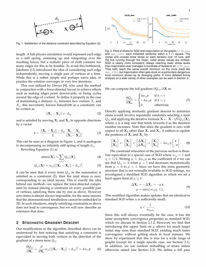
Fig. 1. Satisfaction of the distance constraint described by Equation (2).

length. A full physics simulation would represent each edgeas a stiff spring, summing up and integrating over theresulting forces, but a realistic piece of cloth contains toomany edges for this to be feasible. To avoid this bottleneck,Jakobsen [11] introduced the idea of considering each edgeindependently, moving a single pair of vertices at a time.While this is a rather simple and perhaps naive idea, inpractice the solution converges in very few iterations.

This was utilized by Dwyer [9], who used the methodin conjunction with a force-directed layout to achieve effectssuch as making edges point downwards, or fixing cyclesaround the edge of a wheel. To define it properly in the caseof maintaining a distance dij between two vertices Xi andXj , this movement, known henceforth as a constraint, canbe written as

||Xi −Xj || ← dij (2)

and is satisfied by moving Xi and Xj in opposite directionsby a vector

r =||Xi −Xj || − dij

2

Xi −Xj

||Xi −Xj ||. (3)

This can be seen as a diagram in Figure 1, and is analogousto decompressing an infinitely stiff spring of length dij .

Rewriting Equation (1) as

stress(X) =∑i<j

Qij(X), (4)

Qij(X) = wij(||Xi −Xj || − dij)2, (5)

it can be seen that if every term Qij in the summation issatisfied as a constraint (2), then the total stress is zero,corresponding to an ideal layout. This is exactly the ideabehind our method—we replace the force-directed compo-nent by instead placing a constraint on every possible pairof vertices, satisfying them one by one as above. Howeverzero stress is almost always impossible, for the same reasonsthat the aforementioned tetrahedron cannot be embedded in2D. In such situations, simply satisfying constraints as abovedoes not lead to convergence, but we will now describe anextension that does.

2 STOCHASTIC GRADIENT DESCENT

Our modifications to the algorithm described above can beunderstood by first noticing that satisfying a constraint isequivalent to moving both vertices in the direction of thegradient of a stress term Qij

∂Qij∂Xi

=∂

∂Xiwij(||Xi −Xj || − dij)2 = 4wijr. (6)

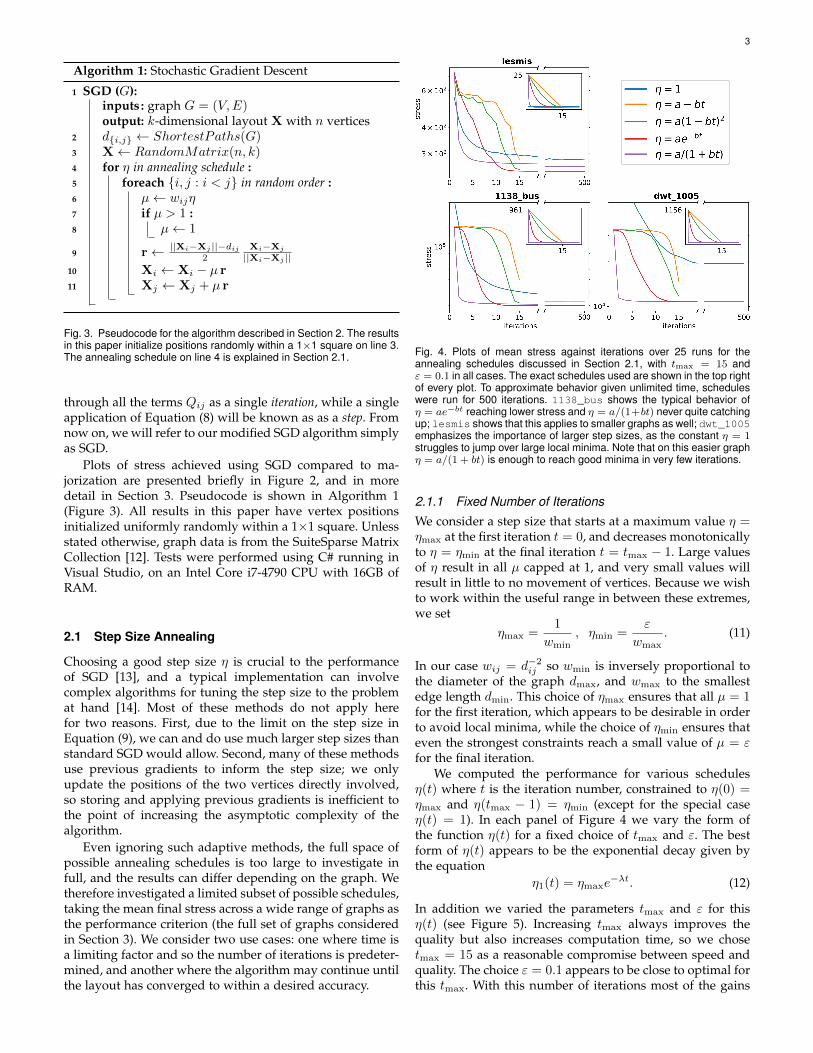
Fig. 2. Plots of stress for SGD and majorization on the graphs 1138_busand dwt_1005, each initialized randomly within a 1×1 square. Thecircles and crosses show stress on each iteration over 10 runs, withthe line running through the mean. Initial stress values are omitted.SGD is clearly more consistent, always reaching lower stress levelsthan majorization ever manages in hundreds of iterations on 1138_bus.They both reach the same overall minimum on the more mesh-likedwt_1005, but majorization often gets stuck on a particularly dangerouslocal minimum, shown by its diverging paths. A more detailed timinganalysis on a wide variety of other examples can be seen in Section 3.

We can compute the full gradient ∂Qij/∂X as

∂Qij∂Xk

=

4wijr if k = i

−4wijr if k = j

0 otherwise.(7)

Directly applying stochastic gradient descent to minimizestress would involve repeatedly randomly selecting a termQij and applying the iterative formula X← X−η∇Qij(X),where η is a step size that tends towards 0 as the iterationnumber increases. Note that since the gradient is zero withrespect to all Xk other than Xi and Xj , it suffices to updatethe positions of Xi and Xj by[

Xi

Xj

]←[Xi

Xj

]+

[∆Xi

∆Xj

]=

[Xi

Xj

]− 4wijη

[r−r

]. (8)

The constraint relaxation of the previous section is there-fore equivalent to a special case of SGD where wij = 1 andη = 1/4. Writing µ = 4wijη as the coefficient of r we cansee that Qij ← 0 when µ = 1 and decreases monotonicallyfrom µ = 0 to µ = 1. Since we have this extra geometricstructure that is not normally available in SGD settings, weinvestigated a modified SGD algorithm in which we set ahard upper limit of µ ≤ 1:

∆Xi = −∆Xj = −µ r,µ = min{wijη, 1 }.

(9)

This modified algorithm makes updates that are identical tostandard SGD when η is sufficiently small,

η <1

wmax. (10)

Since this will always eventually be the case, it has thesame asymptotic convergence properties as standard SGD,which we discuss in Section 2.1.2. However, we find thatintroducing this upper limit on µ allows for much largerinitial step sizes than standard SGD, yielding much fasterconvergence without getting stuck in local minima. Weshow by experiment that this is true for a wide range ofgraphs (except for a single specific case, see Section 3.1).In addition, we use random reshuffling of terms unlessotherwise stated (see Section 2.2). We define a full pass

3

Algorithm 1: Stochastic Gradient Descent

1 SGD (G):inputs : graph G = (V,E)output: k-dimensional layout X with n vertices

2 d{i,j} ← ShortestPaths(G)3 X← RandomMatrix(n, k)4 for η in annealing schedule :5 foreach {i, j : i < j} in random order :6 µ← wijη7 if µ > 1 :8 µ← 1

9 r← ||Xi−Xj ||−dij2

Xi−Xj

||Xi−Xj ||10 Xi ← Xi − µ r11 Xj ← Xj + µ r

Fig. 3. Pseudocode for the algorithm described in Section 2. The resultsin this paper initialize positions randomly within a 1×1 square on line 3.The annealing schedule on line 4 is explained in Section 2.1.

through all the terms Qij as a single iteration, while a singleapplication of Equation (8) will be known as as a step. Fromnow on, we will refer to our modified SGD algorithm simplyas SGD.

Plots of stress achieved using SGD compared to ma-jorization are presented briefly in Figure 2, and in moredetail in Section 3. Pseudocode is shown in Algorithm 1(Figure 3). All results in this paper have vertex positionsinitialized uniformly randomly within a 1×1 square. Unlessstated otherwise, graph data is from the SuiteSparse MatrixCollection [12]. Tests were performed using C# running inVisual Studio, on an Intel Core i7-4790 CPU with 16GB ofRAM.

2.1 Step Size Annealing

Choosing a good step size η is crucial to the performanceof SGD [13], and a typical implementation can involvecomplex algorithms for tuning the step size to the problemat hand [14]. Most of these methods do not apply herefor two reasons. First, due to the limit on the step size inEquation (9), we can and do use much larger step sizes thanstandard SGD would allow. Second, many of these methodsuse previous gradients to inform the step size; we onlyupdate the positions of the two vertices directly involved,so storing and applying previous gradients is inefficient tothe point of increasing the asymptotic complexity of thealgorithm.

Even ignoring such adaptive methods, the full space ofpossible annealing schedules is too large to investigate infull, and the results can differ depending on the graph. Wetherefore investigated a limited subset of possible schedules,taking the mean final stress across a wide range of graphs asthe performance criterion (the full set of graphs consideredin Section 3). We consider two use cases: one where time isa limiting factor and so the number of iterations is predeter-mined, and another where the algorithm may continue untilthe layout has converged to within a desired accuracy.

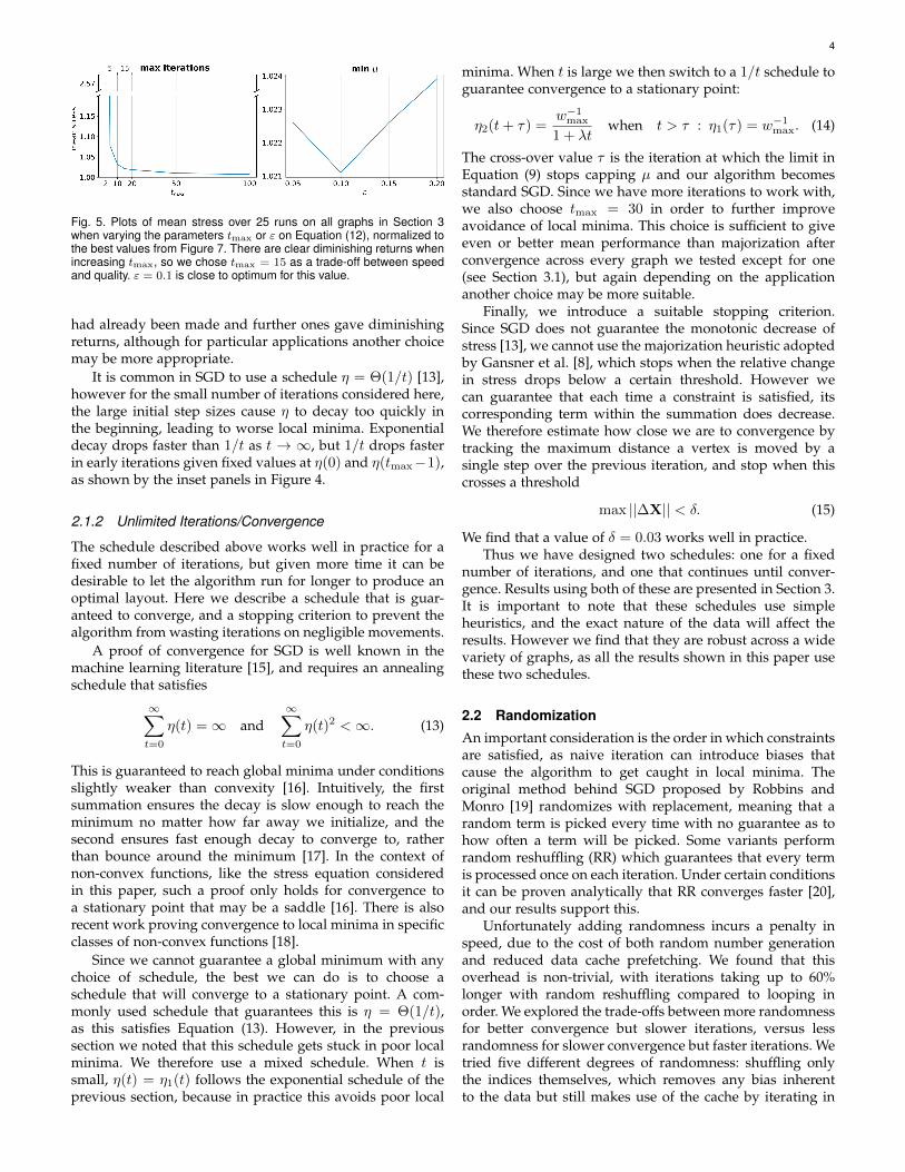
Fig. 4. Plots of mean stress against iterations over 25 runs for theannealing schedules discussed in Section 2.1, with tmax = 15 andε = 0.1 in all cases. The exact schedules used are shown in the top rightof every plot. To approximate behavior given unlimited time, scheduleswere run for 500 iterations. 1138_bus shows the typical behavior ofη = ae−bt reaching lower stress and η = a/(1+bt) never quite catchingup; lesmis shows that this applies to smaller graphs as well; dwt_1005emphasizes the importance of larger step sizes, as the constant η = 1struggles to jump over large local minima. Note that on this easier graphη = a/(1 + bt) is enough to reach good minima in very few iterations.

2.1.1 Fixed Number of Iterations

We consider a step size that starts at a maximum value η =ηmax at the first iteration t = 0, and decreases monotonicallyto η = ηmin at the final iteration t = tmax − 1. Large valuesof η result in all µ capped at 1, and very small values willresult in little to no movement of vertices. Because we wishto work within the useful range in between these extremes,we set

ηmax =1

wmin, ηmin =

ε

wmax. (11)

In our case wij = d−2ij so wmin is inversely proportional tothe diameter of the graph dmax, and wmax to the smallestedge length dmin. This choice of ηmax ensures that all µ = 1for the first iteration, which appears to be desirable in orderto avoid local minima, while the choice of ηmin ensures thateven the strongest constraints reach a small value of µ = εfor the final iteration.

We computed the performance for various schedulesη(t) where t is the iteration number, constrained to η(0) =ηmax and η(tmax − 1) = ηmin (except for the special caseη(t) = 1). In each panel of Figure 4 we vary the form ofthe function η(t) for a fixed choice of tmax and ε. The bestform of η(t) appears to be the exponential decay given bythe equation

η1(t) = ηmaxe−λt. (12)

In addition we varied the parameters tmax and ε for thisη(t) (see Figure 5). Increasing tmax always improves thequality but also increases computation time, so we chosetmax = 15 as a reasonable compromise between speed andquality. The choice ε = 0.1 appears to be close to optimal forthis tmax. With this number of iterations most of the gains

4

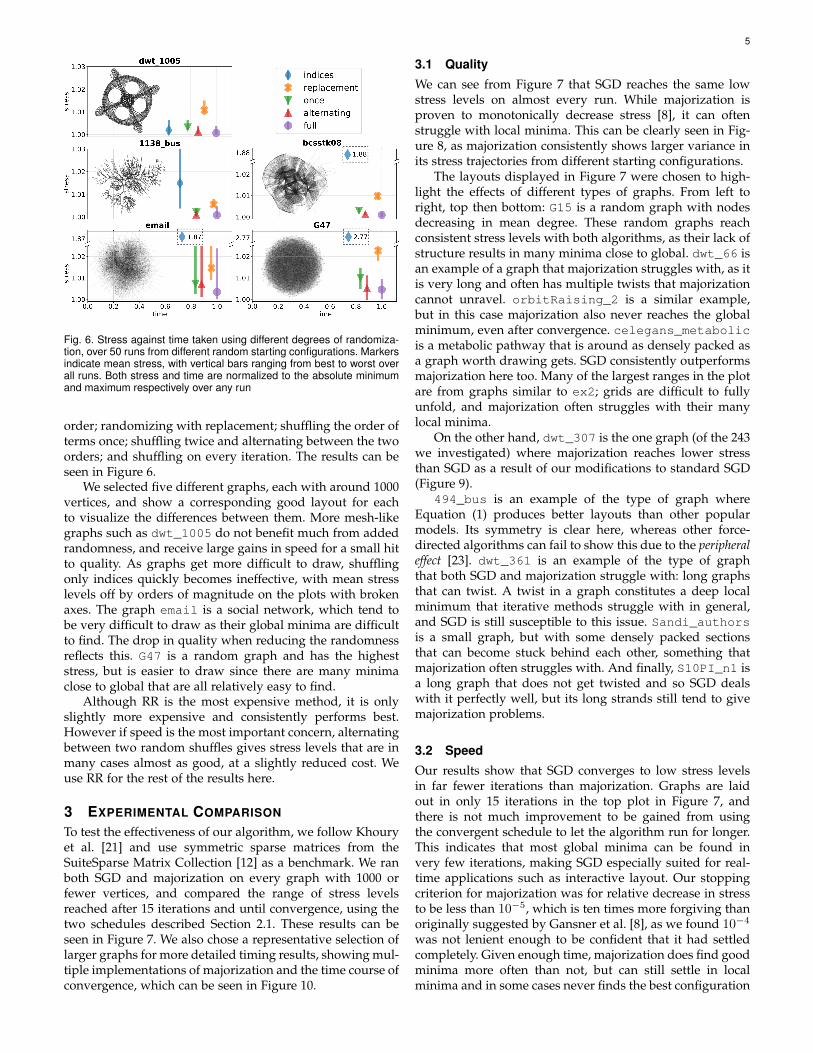
Fig. 5. Plots of mean stress over 25 runs on all graphs in Section 3when varying the parameters tmax or ε on Equation (12), normalized tothe best values from Figure 7. There are clear diminishing returns whenincreasing tmax, so we chose tmax = 15 as a trade-off between speedand quality. ε = 0.1 is close to optimum for this value.

had already been made and further ones gave diminishingreturns, although for particular applications another choicemay be more appropriate.

It is common in SGD to use a schedule η = Θ(1/t) [13],however for the small number of iterations considered here,the large initial step sizes cause η to decay too quickly inthe beginning, leading to worse local minima. Exponentialdecay drops faster than 1/t as t → ∞, but 1/t drops fasterin early iterations given fixed values at η(0) and η(tmax−1),as shown by the inset panels in Figure 4.

2.1.2 Unlimited Iterations/Convergence

The schedule described above works well in practice for afixed number of iterations, but given more time it can bedesirable to let the algorithm run for longer to produce anoptimal layout. Here we describe a schedule that is guar-anteed to converge, and a stopping criterion to prevent thealgorithm from wasting iterations on negligible movements.

A proof of convergence for SGD is well known in themachine learning literature [15], and requires an annealingschedule that satisfies

∞∑t=0

η(t) =∞ and∞∑t=0

η(t)2 <∞. (13)

This is guaranteed to reach global minima under conditionsslightly weaker than convexity [16]. Intuitively, the firstsummation ensures the decay is slow enough to reach theminimum no matter how far away we initialize, and thesecond ensures fast enough decay to converge to, ratherthan bounce around the minimum [17]. In the context ofnon-convex functions, like the stress equation consideredin this paper, such a proof only holds for convergence toa stationary point that may be a saddle [16]. There is alsorecent work proving convergence to local minima in specificclasses of non-convex functions [18].

Since we cannot guarantee a global minimum with anychoice of schedule, the best we can do is to choose aschedule that will converge to a stationary point. A com-monly used schedule that guarantees this is η = Θ(1/t),as this satisfies Equation (13). However, in the previoussection we noted that this schedule gets stuck in poor localminima. We therefore use a mixed schedule. When t issmall, η(t) = η1(t) follows the exponential schedule of theprevious section, because in practice this avoids poor local

minima. When t is large we then switch to a 1/t schedule toguarantee convergence to a stationary point:

η2(t+ τ) =w−1max

1 + λtwhen t > τ : η1(τ) = w−1max. (14)

The cross-over value τ is the iteration at which the limit inEquation (9) stops capping µ and our algorithm becomesstandard SGD. Since we have more iterations to work with,we also choose tmax = 30 in order to further improveavoidance of local minima. This choice is sufficient to giveeven or better mean performance than majorization afterconvergence across every graph we tested except for one(see Section 3.1), but again depending on the applicationanother choice may be more suitable.

Finally, we introduce a suitable stopping criterion.Since SGD does not guarantee the monotonic decrease ofstress [13], we cannot use the majorization heuristic adoptedby Gansner et al. [8], which stops when the relative changein stress drops below a certain threshold. However wecan guarantee that each time a constraint is satisfied, itscorresponding term within the summation does decrease.We therefore estimate how close we are to convergence bytracking the maximum distance a vertex is moved by asingle step over the previous iteration, and stop when thiscrosses a threshold

max ||∆X|| < δ. (15)

We find that a value of δ = 0.03 works well in practice.Thus we have designed two schedules: one for a fixed

number of iterations, and one that continues until conver-gence. Results using both of these are presented in Section 3.It is important to note that these schedules use simpleheuristics, and the exact nature of the data will affect theresults. However we find that they are robust across a widevariety of graphs, as all the results shown in this paper usethese two schedules.

2.2 Randomization

An important consideration is the order in which constraintsare satisfied, as naive iteration can introduce biases thatcause the algorithm to get caught in local minima. Theoriginal method behind SGD proposed by Robbins andMonro [19] randomizes with replacement, meaning that arandom term is picked every time with no guarantee as tohow often a term will be picked. Some variants performrandom reshuffling (RR) which guarantees that every termis processed once on each iteration. Under certain conditionsit can be proven analytically that RR converges faster [20],and our results support this.

Unfortunately adding randomness incurs a penalty inspeed, due to the cost of both random number generationand reduced data cache prefetching. We found that thisoverhead is non-trivial, with iterations taking up to 60%longer with random reshuffling compared to looping inorder. We explored the trade-offs between more randomnessfor better convergence but slower iterations, versus lessrandomness for slower convergence but faster iterations. Wetried five different degrees of randomness: shuffling onlythe indices themselves, which removes any bias inherentto the data but still makes use of the cache by iterating in

5

Fig. 6. Stress against time taken using different degrees of randomiza-tion, over 50 runs from different random starting configurations. Markersindicate mean stress, with vertical bars ranging from best to worst overall runs. Both stress and time are normalized to the absolute minimumand maximum respectively over any run

order; randomizing with replacement; shuffling the order ofterms once; shuffling twice and alternating between the twoorders; and shuffling on every iteration. The results can beseen in Figure 6.

We selected five different graphs, each with around 1000vertices, and show a corresponding good layout for eachto visualize the differences between them. More mesh-likegraphs such as dwt_1005 do not benefit much from addedrandomness, and receive large gains in speed for a small hitto quality. As graphs get more difficult to draw, shufflingonly indices quickly becomes ineffective, with mean stresslevels off by orders of magnitude on the plots with brokenaxes. The graph email is a social network, which tend tobe very difficult to draw as their global minima are difficultto find. The drop in quality when reducing the randomnessreflects this. G47 is a random graph and has the higheststress, but is easier to draw since there are many minimaclose to global that are all relatively easy to find.

Although RR is the most expensive method, it is onlyslightly more expensive and consistently performs best.However if speed is the most important concern, alternatingbetween two random shuffles gives stress levels that are inmany cases almost as good, at a slightly reduced cost. Weuse RR for the rest of the results here.

3 EXPERIMENTAL COMPARISON

To test the effectiveness of our algorithm, we follow Khouryet al. [21] and use symmetric sparse matrices from theSuiteSparse Matrix Collection [12] as a benchmark. We ranboth SGD and majorization on every graph with 1000 orfewer vertices, and compared the range of stress levelsreached after 15 iterations and until convergence, using thetwo schedules described Section 2.1. These results can beseen in Figure 7. We also chose a representative selection oflarger graphs for more detailed timing results, showing mul-tiple implementations of majorization and the time course ofconvergence, which can be seen in Figure 10.

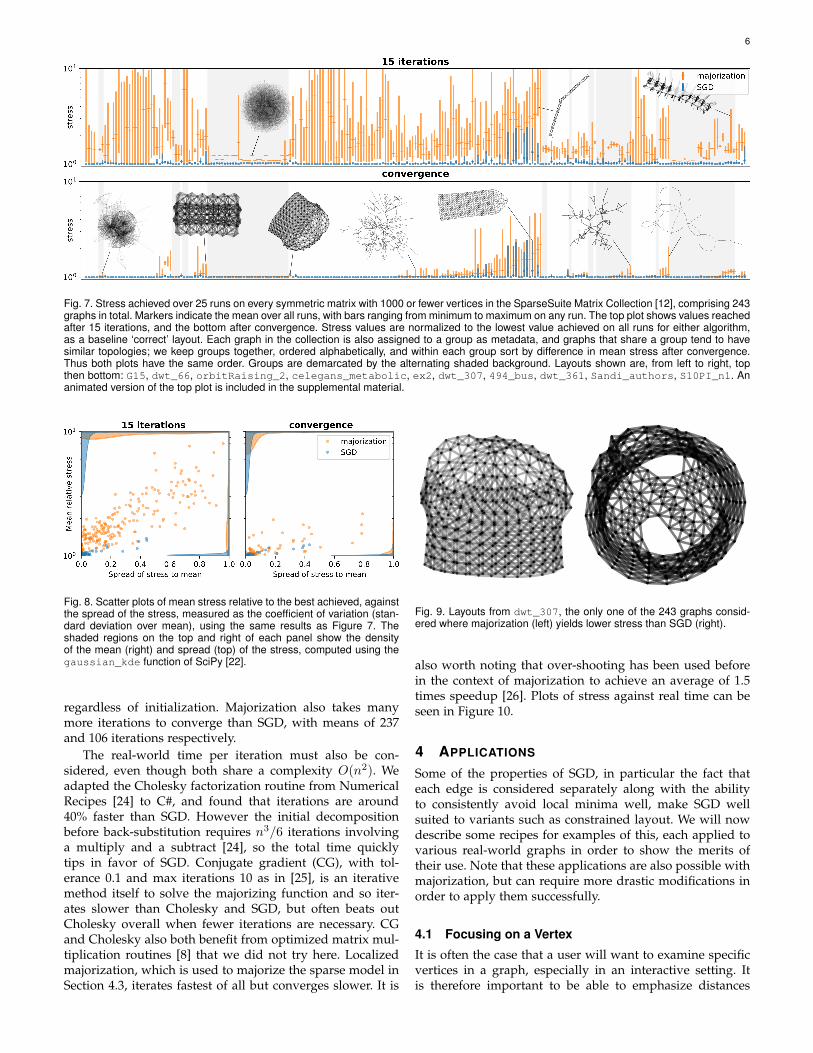
3.1 QualityWe can see from Figure 7 that SGD reaches the same lowstress levels on almost every run. While majorization isproven to monotonically decrease stress [8], it can oftenstruggle with local minima. This can be clearly seen in Fig-ure 8, as majorization consistently shows larger variance inits stress trajectories from different starting configurations.

The layouts displayed in Figure 7 were chosen to high-light the effects of different types of graphs. From left toright, top then bottom: G15 is a random graph with nodesdecreasing in mean degree. These random graphs reachconsistent stress levels with both algorithms, as their lack ofstructure results in many minima close to global. dwt_66 isan example of a graph that majorization struggles with, as itis very long and often has multiple twists that majorizationcannot unravel. orbitRaising_2 is a similar example,but in this case majorization also never reaches the globalminimum, even after convergence. celegans_metabolicis a metabolic pathway that is around as densely packed asa graph worth drawing gets. SGD consistently outperformsmajorization here too. Many of the largest ranges in the plotare from graphs similar to ex2; grids are difficult to fullyunfold, and majorization often struggles with their manylocal minima.

On the other hand, dwt_307 is the one graph (of the 243we investigated) where majorization reaches lower stressthan SGD as a result of our modifications to standard SGD(Figure 9).

494_bus is an example of the type of graph whereEquation (1) produces better layouts than other popularmodels. Its symmetry is clear here, whereas other force-directed algorithms can fail to show this due to the peripheraleffect [23]. dwt_361 is an example of the type of graphthat both SGD and majorization struggle with: long graphsthat can twist. A twist in a graph constitutes a deep localminimum that iterative methods struggle with in general,and SGD is still susceptible to this issue. Sandi_authorsis a small graph, but with some densely packed sectionsthat can become stuck behind each other, something thatmajorization often struggles with. And finally, S10PI_n1 isa long graph that does not get twisted and so SGD dealswith it perfectly well, but its long strands still tend to givemajorization problems.

3.2 SpeedOur results show that SGD converges to low stress levelsin far fewer iterations than majorization. Graphs are laidout in only 15 iterations in the top plot in Figure 7, andthere is not much improvement to be gained from usingthe convergent schedule to let the algorithm run for longer.This indicates that most global minima can be found invery few iterations, making SGD especially suited for real-time applications such as interactive layout. Our stoppingcriterion for majorization was for relative decrease in stressto be less than 10−5, which is ten times more forgiving thanoriginally suggested by Gansner et al. [8], as we found 10−4

was not lenient enough to be confident that it had settledcompletely. Given enough time, majorization does find goodminima more often than not, but can still settle in localminima and in some cases never finds the best configuration

6

Fig. 7. Stress achieved over 25 runs on every symmetric matrix with 1000 or fewer vertices in the SparseSuite Matrix Collection [12], comprising 243graphs in total. Markers indicate the mean over all runs, with bars ranging from minimum to maximum on any run. The top plot shows values reachedafter 15 iterations, and the bottom after convergence. Stress values are normalized to the lowest value achieved on all runs for either algorithm,as a baseline ‘correct’ layout. Each graph in the collection is also assigned to a group as metadata, and graphs that share a group tend to havesimilar topologies; we keep groups together, ordered alphabetically, and within each group sort by difference in mean stress after convergence.Thus both plots have the same order. Groups are demarcated by the alternating shaded background. Layouts shown are, from left to right, topthen bottom: G15, dwt_66, orbitRaising_2, celegans_metabolic, ex2, dwt_307, 494_bus, dwt_361, Sandi_authors, S10PI_n1. Ananimated version of the top plot is included in the supplemental material.

Fig. 8. Scatter plots of mean stress relative to the best achieved, againstthe spread of the stress, measured as the coefficient of variation (stan-dard deviation over mean), using the same results as Figure 7. Theshaded regions on the top and right of each panel show the densityof the mean (right) and spread (top) of the stress, computed using thegaussian_kde function of SciPy [22].

regardless of initialization. Majorization also takes manymore iterations to converge than SGD, with means of 237and 106 iterations respectively.

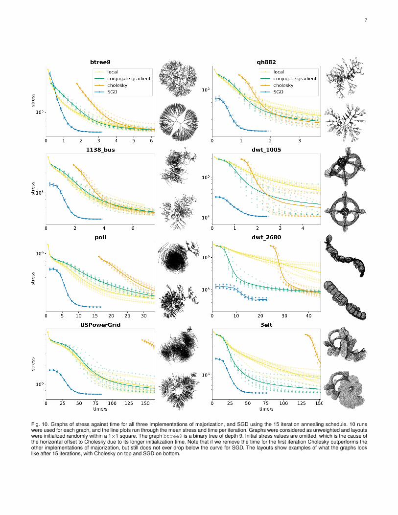
The real-world time per iteration must also be con-sidered, even though both share a complexity O(n2). Weadapted the Cholesky factorization routine from NumericalRecipes [24] to C#, and found that iterations are around40% faster than SGD. However the initial decompositionbefore back-substitution requires n3/6 iterations involvinga multiply and a subtract [24], so the total time quicklytips in favor of SGD. Conjugate gradient (CG), with tol-erance 0.1 and max iterations 10 as in [25], is an iterativemethod itself to solve the majorizing function and so iter-ates slower than Cholesky and SGD, but often beats outCholesky overall when fewer iterations are necessary. CGand Cholesky also both benefit from optimized matrix mul-tiplication routines [8] that we did not try here. Localizedmajorization, which is used to majorize the sparse model inSection 4.3, iterates fastest of all but converges slower. It is

Fig. 9. Layouts from dwt_307, the only one of the 243 graphs consid-ered where majorization (left) yields lower stress than SGD (right).

also worth noting that over-shooting has been used beforein the context of majorization to achieve an average of 1.5times speedup [26]. Plots of stress against real time can beseen in Figure 10.

4 APPLICATIONS

Some of the properties of SGD, in particular the fact thateach edge is considered separately along with the abilityto consistently avoid local minima well, make SGD wellsuited to variants such as constrained layout. We will nowdescribe some recipes for examples of this, each applied tovarious real-world graphs in order to show the merits oftheir use. Note that these applications are also possible withmajorization, but can require more drastic modifications inorder to apply them successfully.

4.1 Focusing on a Vertex

It is often the case that a user will want to examine specificvertices in a graph, especially in an interactive setting. Itis therefore important to be able to emphasize distances

7

Fig. 10. Graphs of stress against time for all three implementations of majorization, and SGD using the 15 iteration annealing schedule. 10 runswere used for each graph, and the line plots run through the mean stress and time per iteration. Graphs were considered as unweighted and layoutswere initialized randomly within a 1×1 square. The graph btree9 is a binary tree of depth 9. Initial stress values are omitted, which is the cause ofthe horizontal offset to Cholesky due to its longer initialization time. Note that if we remove the time for the first iteration Cholesky outperforms theother implementations of majorization, but still does not ever drop below the curve for SGD. The layouts show examples of what the graphs looklike after 15 iterations, with Cholesky on top and SGD on bottom.

8

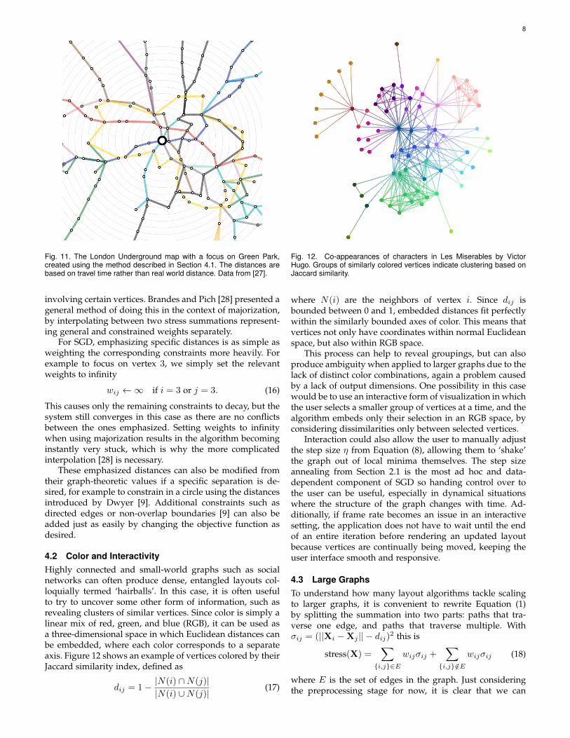
Fig. 11. The London Underground map with a focus on Green Park,created using the method described in Section 4.1. The distances arebased on travel time rather than real world distance. Data from [27].

involving certain vertices. Brandes and Pich [28] presented ageneral method of doing this in the context of majorization,by interpolating between two stress summations represent-ing general and constrained weights separately.

For SGD, emphasizing specific distances is as simple asweighting the corresponding constraints more heavily. Forexample to focus on vertex 3, we simply set the relevantweights to infinity

wij ←∞ if i = 3 or j = 3. (16)

This causes only the remaining constraints to decay, but thesystem still converges in this case as there are no conflictsbetween the ones emphasized. Setting weights to infinitywhen using majorization results in the algorithm becominginstantly very stuck, which is why the more complicatedinterpolation [28] is necessary.

These emphasized distances can also be modified fromtheir graph-theoretic values if a specific separation is de-sired, for example to constrain in a circle using the distancesintroduced by Dwyer [9]. Additional constraints such asdirected edges or non-overlap boundaries [9] can also beadded just as easily by changing the objective function asdesired.

4.2 Color and InteractivityHighly connected and small-world graphs such as socialnetworks can often produce dense, entangled layouts col-loquially termed ‘hairballs’. In this case, it is often usefulto try to uncover some other form of information, such asrevealing clusters of similar vertices. Since color is simply alinear mix of red, green, and blue (RGB), it can be used asa three-dimensional space in which Euclidean distances canbe embedded, where each color corresponds to a separateaxis. Figure 12 shows an example of vertices colored by theirJaccard similarity index, defined as

dij = 1− |N(i) ∩N(j)||N(i) ∪N(j)|

(17)

Fig. 12. Co-appearances of characters in Les Miserables by VictorHugo. Groups of similarly colored vertices indicate clustering based onJaccard similarity.

where N(i) are the neighbors of vertex i. Since dij isbounded between 0 and 1, embedded distances fit perfectlywithin the similarly bounded axes of color. This means thatvertices not only have coordinates within normal Euclideanspace, but also within RGB space.

This process can help to reveal groupings, but can alsoproduce ambiguity when applied to larger graphs due to thelack of distinct color combinations, again a problem causedby a lack of output dimensions. One possibility in this casewould be to use an interactive form of visualization in whichthe user selects a smaller group of vertices at a time, and thealgorithm embeds only their selection in an RGB space, byconsidering dissimilarities only between selected vertices.

Interaction could also allow the user to manually adjustthe step size η from Equation (8), allowing them to ‘shake’the graph out of local minima themselves. The step sizeannealing from Section 2.1 is the most ad hoc and data-dependent component of SGD so handing control over tothe user can be useful, especially in dynamical situationswhere the structure of the graph changes with time. Ad-ditionally, if frame rate becomes an issue in an interactivesetting, the application does not have to wait until the endof an entire iteration before rendering an updated layoutbecause vertices are continually being moved, keeping theuser interface smooth and responsive.

4.3 Large GraphsTo understand how many layout algorithms tackle scalingto larger graphs, it is convenient to rewrite Equation (1)by splitting the summation into two parts: paths that tra-verse one edge, and paths that traverse multiple. Withσij = (||Xi −Xj || − dij)2 this is

stress(X) =∑{i,j}∈E

wijσij +∑{i,j}/∈E

wijσij (18)

where E is the set of edges in the graph. Just consideringthe preprocessing stage for now, it is clear that we can

9

easily compute d and w for the first half of the summationdirectly from the graph. Real-world graphs are also usuallysparse, so for a graph with n vertices and m edges, m� n2

making the space required to store these values tolerable.However the second half is not so easy—an all-pairs shortestpaths (APSP) calculation takes O(m + n) time per vertexfor an unweighted graph with a breadth-first search, orO(m + n log n) for a weighted graph using Dijkstra’s algo-rithm [29]. Combined with requiringO(n2) space to store allthe values of dij , this makes the preprocessing stage aloneintractable for large graphs.

The second stage is iteration, where the layout is gradu-ally improved towards a good minimum. Again, computingthe first summation is tolerable, but the number of longerdistance contributions quickly grows out of control. Manynotable attempts have been made at tackling this secondhalf. A common approach is to ignore dij , and to ap-proximate the summation as an n-body repulsion problem,which can be efficiently well approximated using k-d trees[30]. Hu [23] and independently Hachul and Junger [31]used this in the context of the force-directed model ofFruchterman and Reingold [32], along with a multilevelcoarsening scheme to avoid local minima. Gansner et al. [25]use it with majorization by summing over−α log ||Xi−Xj ||instead. Brandes and Pich [33] even ignore the second halfcompletely and capture the long-range structure by firstinitializing with a fast approximation to classical scaling [3],which minimizes the inner product rather than Euclideandistance.

There are a couple of issues with this idea, one beingthat treating all long-range forces equally is unfaithful tograph-theoretic distances, and another being that the rela-tive strength of these forces depends on an extra parameterthat can strongly affect the final layout of the graph [23].Keeping these dependent on their graph-theoretic distancesidesteps both of these issues, but brings back the problemof computing and storing shortest paths. One approach tomaintaining this dependence comes from Khoury et al. [21],who use a low-rank approximation of the distance matrixbased on its singular value decomposition. This can workextremely well, but still requires APSP unless wij = d−1ij .

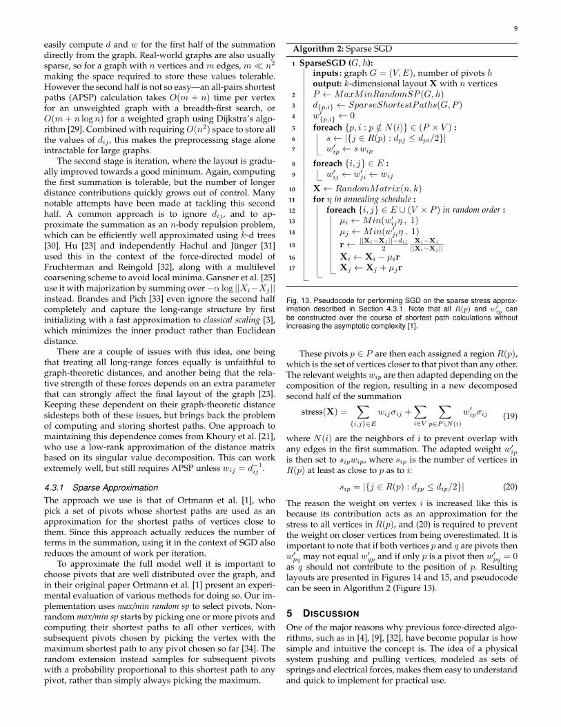
4.3.1 Sparse ApproximationThe approach we use is that of Ortmann et al. [1], whopick a set of pivots whose shortest paths are used as anapproximation for the shortest paths of vertices close tothem. Since this approach actually reduces the number ofterms in the summation, using it in the context of SGD alsoreduces the amount of work per iteration.

To approximate the full model well it is important tochoose pivots that are well distributed over the graph, andin their original paper Ortmann et al. [1] present an experi-mental evaluation of various methods for doing so. Our im-plementation uses max/min random sp to select pivots. Non-random max/min sp starts by picking one or more pivots andcomputing their shortest paths to all other vertices, withsubsequent pivots chosen by picking the vertex with themaximum shortest path to any pivot chosen so far [34]. Therandom extension instead samples for subsequent pivotswith a probability proportional to this shortest path to anypivot, rather than simply always picking the maximum.

Algorithm 2: Sparse SGD

1 SparseSGD (G, h):inputs : graph G = (V,E), number of pivots houtput: k-dimensional layout X with n vertices

2 P ←MaxMinRandomSP (G, h)3 d{p,i} ← SparseShortestPaths(G,P )4 w′{p,i} ← 0

5 foreach {p, i : p /∈ N(i)} ∈ (P × V ) :6 s← |{j ∈ R(p) : dpj ≤ dpi/2}|7 w′ip ← swip

8 foreach {i, j} ∈ E :9 w′ij ← w′ji ← wij

10 X← RandomMatrix(n, k)11 for η in annealing schedule :12 foreach {i, j} ∈ E ∪ (V × P ) in random order :13 µi ←Min(w′ijη , 1)14 µj ←Min(w′jiη , 1)

15 r← ||Xi−Xj ||−dij2

Xi−Xj

||Xi−Xj ||16 Xi ← Xi − µir17 Xj ← Xj + µjr

Fig. 13. Pseudocode for performing SGD on the sparse stress approx-imation described in Section 4.3.1. Note that all R(p) and w′ip canbe constructed over the course of shortest path calculations withoutincreasing the asymptotic complexity [1].

These pivots p ∈ P are then each assigned a region R(p),which is the set of vertices closer to that pivot than any other.The relevant weightswip are then adapted depending on thecomposition of the region, resulting in a new decomposedsecond half of the summation

stress(X) =∑{i,j}∈E

wijσij +∑i∈V

∑p∈P\N(i)

w′ipσij (19)

where N(i) are the neighbors of i to prevent overlap withany edges in the first summation. The adapted weight w′ipis then set to sipwip, where sip is the number of vertices inR(p) at least as close to p as to i:

sip = |{j ∈ R(p) : djp ≤ dip/2}| (20)

The reason the weight on vertex i is increased like this isbecause its contribution acts as an approximation for thestress to all vertices in R(p), and (20) is required to preventthe weight on closer vertices from being overestimated. It isimportant to note that if both vertices p and q are pivots thenw′pq may not equal w′qp and if only p is a pivot then w′pq = 0as q should not contribute to the position of p. Resultinglayouts are presented in Figures 14 and 15, and pseudocodecan be seen in Algorithm 2 (Figure 13).

5 DISCUSSION

One of the major reasons why previous force-directed algo-rithms, such as in [4], [9], [32], have become popular is howsimple and intuitive the concept is. The idea of a physicalsystem pushing and pulling vertices, modeled as sets ofsprings and electrical forces, makes them easy to understandand quick to implement for practical use.

10

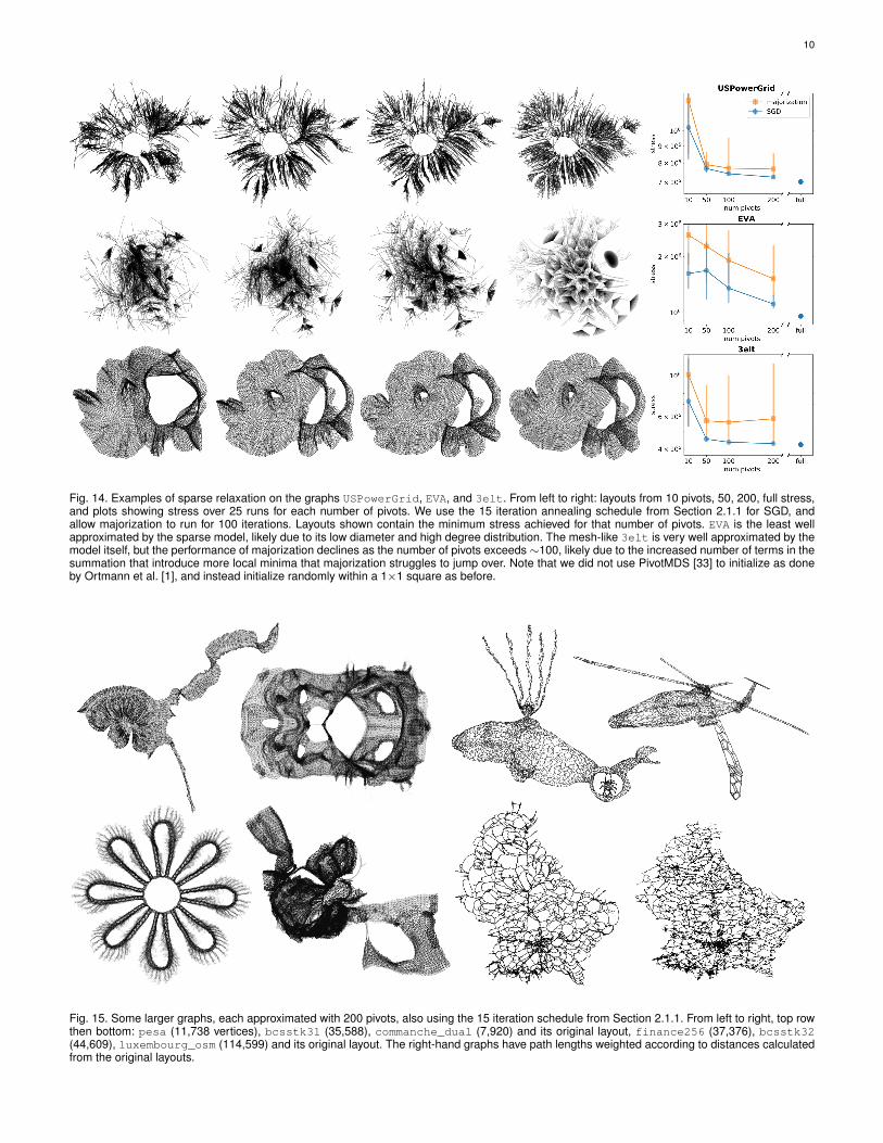
Fig. 14. Examples of sparse relaxation on the graphs USPowerGrid, EVA, and 3elt. From left to right: layouts from 10 pivots, 50, 200, full stress,and plots showing stress over 25 runs for each number of pivots. We use the 15 iteration annealing schedule from Section 2.1.1 for SGD, andallow majorization to run for 100 iterations. Layouts shown contain the minimum stress achieved for that number of pivots. EVA is the least wellapproximated by the sparse model, likely due to its low diameter and high degree distribution. The mesh-like 3elt is very well approximated by themodel itself, but the performance of majorization declines as the number of pivots exceeds ∼100, likely due to the increased number of terms in thesummation that introduce more local minima that majorization struggles to jump over. Note that we did not use PivotMDS [33] to initialize as doneby Ortmann et al. [1], and instead initialize randomly within a 1×1 square as before.

Fig. 15. Some larger graphs, each approximated with 200 pivots, also using the 15 iteration schedule from Section 2.1.1. From left to right, top rowthen bottom: pesa (11,738 vertices), bcsstk31 (35,588), commanche_dual (7,920) and its original layout, finance256 (37,376), bcsstk32(44,609), luxembourg_osm (114,599) and its original layout. The right-hand graphs have path lengths weighted according to distances calculatedfrom the original layouts.

11

The geometric interpretation of the SGD algorithm wehave presented shares these qualities, as the concept ofmoving pairs of vertices one by one towards an idealdistance is just as simple. In fact the stress formulation (1)is commonly known as the spring model [4], [23], and thephysical analogy of decompressing one spring at a timevery naturally fits this intuition. The implementation alsorequires no equation solver, and there is no need to considersmart initialization, which can often be just as complex atask [3]. Considering only a single pair of vertices at a timealso makes further constrained layouts easy to implement,and allows an appropriate sparse approximation to grantscalability up to large graphs.

But perhaps the most important benefit of SGD is itsconsistency regardless of initialization, despite being non-deterministic due to the shuffling of the order of terms. Bycontrast, the plots in Section 3 clearly show how vastly theresults from majorization can differ depending on initial-ization, especially when restricted to a limited number ofiterations. This reliability of SGD can be crucial for real-timeapplications with fixed limits on computation time, such aswithin an interactive visualization.

However there are still situations where SGD can strug-gle with local minima, such as dwt_2680 which is sus-ceptible to twisting in the middle. This can be seen inFigure 10 where we purposefully included a twisted layoutto illustrate this pitfall. A potential solution to this is over-shooting, or in other words allowing values of 0 < µ < 2 inEquation (9). This greatly reduces the chance of a twist, butresults in poorer local minima in most other cases and canalso bring back the problem of divergence, so is a potentialavenue for future work, perhaps to be used in conjunctionwith an adaptive annealing schedule to further optimizeperformance depending on the input data.

5.1 Conclusion

In this paper we have presented a modified version ofstochastic gradient descent (SGD) to minimize stress asdefined by Equation (1). An investigation comparing themethod to majorization shows consistently faster conver-gence to lower stress levels, and the fact that only a sin-gle pair of vertices is considered at a time makes it wellsuited for variants such as constrained layout or the pivot-based approximation of Ortmann et al. [1]. This improvedperformance—combined with a simplicity that forgoes anequation solver or smart initialization—makes SGD a strongcandidate for general graph layout applications.

Code used for timing experiments, along with someexample Jupyter notebooks, is open source and availableat www.github.com/jxz12/s gd2.

ACKNOWLEDGMENTS

We thank Tim Davis and Yifan Hu for maintaining theSuiteSparse Matrix Collection [12], where most of the graphdata used in this paper was obtained. We are also gratefulto the anonymous reviewers whose comments helped us toimprove the paper.

REFERENCES

[1] M. Ortmann, M. Klimenta, and U. Brandes, “A sparse stressmodel,” Journal of Graph Algorithms and Applications, vol. 21, no. 5,pp. 791–821, 2017.

[2] T. F. Cox and M. A. A. Cox, Multidimensional Scaling. CRC press,2000.

[3] U. Brandes and C. Pich, “An experimental study on distance-basedgraph drawing,” in Graph Drawing. Springer, 2009, pp. 218–229.

[4] T. Kamada and S. Kawai, “An algorithm for drawing generalundirected graphs,” Information Processing Letters, vol. 31, no. 1,pp. 7–15, 1989.

[5] J. B. Kruskal, “Multidimensional scaling by optimizing goodnessof fit to a nonmetric hypothesis,” Psychometrika, vol. 29, no. 1, pp.1–27, 1964.

[6] ——, “Nonmetric multidimensional scaling: a numerical method,”Psychometrika, vol. 29, no. 2, pp. 115–129, 1964.

[7] J. De Leeuw, “Convergence of the majorization method for mul-tidimensional scaling,” Journal of Classification, vol. 5, no. 2, pp.163–180, 1988.

[8] E. R. Gansner, Y. Koren, and S. North, “Graph drawing by stressmajorization,” in Graph Drawing. Springer, 2005, pp. 239–250.

[9] T. Dwyer, “Scalable, versatile and simple constrained graph lay-out,” in Computer Graphics Forum, vol. 28, no. 3. Wiley OnlineLibrary, 2009, pp. 991–998.

[10] M. Bostock, V. Ogievetsky, and J. Heer, “D3 data-driven docu-ments,” IEEE Transactions on Visualization and Computer Graphics,vol. 17, no. 12, pp. 2301–2309, 2011.

[11] T. Jakobsen, “Advanced character physics,” in Game DevelopersConference, vol. 3, 2001, pp. 383–401.

[12] T. A. Davis and Y. Hu, “The University of Florida sparse matrixcollection,” ACM Transactions on Mathematical Software (TOMS),vol. 38, no. 1, pp. 1:1–1:25, 2011.

[13] C. Darken, J. Chang, and J. Moody, “Learning rate schedules forfaster stochastic gradient search,” in Neural Networks for SignalProcessing II Proceedings of the 1992 IEEE Workshop. IEEE, 1992,pp. 3–12.

[14] S. Ruder, “An overview of gradient descent optimization algo-rithms,” arXiv:1609.04747, 2016.

[15] L. Bottou, “Stochastic gradient descent tricks,” in Neural Networks:Tricks of the Trade. Springer, 2012, pp. 421–436.

[16] ——, “Online learning and stochastic approximations,” in On-lineLearning in Neural Networks. Cambridge University Press, 1999,pp. 9–42.

[17] M. Welling and Y. W. Teh, “Bayesian learning via stochasticgradient langevin dynamics,” in Proceedings of the 28th InternationalConference on Machine Learning, 2011, pp. 681–688.

[18] R. Ge, F. Huang, C. Jin, and Y. Yuan, “Escaping from saddlepoints—online stochastic gradient for tensor decomposition,” inConference on Learning Theory, 2015, pp. 797–842.

[19] H. Robbins and S. Monro, “A stochastic approximation method,”The Annals of Mathematical Statistics, vol. 22, no. 3, pp. 400–407,1951.

[20] M. Gurbuzbalaban, A. Ozdaglar, and P. Parrilo, “Why randomreshuffling beats stochastic gradient descent,” arXiv:1510.08560,2015.

[21] M. Khoury, Y. Hu, S. Krishnan, and C. Scheidegger, “Drawinglarge graphs by low-rank stress majorization,” in Computer Graph-ics Forum, vol. 31, no. 3pt1. Wiley Online Library, 2012, pp. 975–984.

[22] E. Jones, T. Oliphant, P. Peterson et al., “SciPy: Open sourcescientific tools for Python,” 2001–, accessed 10/04/2018. [Online].Available: http://www.scipy.org/

[23] Y. Hu, “Efficient, high-quality force-directed graph drawing,”Mathematica Journal, vol. 10, no. 1, pp. 37–71, 2005.

[24] W. H. Press, S. A. Teukolsky, W. T. Vetterling, and B. P. Flannery,Numerical recipes in C. Cambridge University Press, 1996.

[25] E. R. Gansner, Y. Hu, and S. North, “A maxent-stress model forgraph layout,” in IEEE Transactions on Visualization and ComputerGraphics, vol. 19, no. 6. IEEE, 2013, pp. 927–940.

[26] Y. Wang and Z. Wang, “A fast successive over-relaxation algorithmfor force-directed network graph drawing,” Science China Informa-tion Sciences, vol. 55, no. 3, pp. 677–688, 2012.

[27] P. Trotman, “London underground travel time map,” 2016,accessed 28/08/2017. [Online]. Available: https://github.com/petertrotman/london-underground-travel-time-map

[28] U. Brandes and C. Pich, “More flexible radial layout,” Journal ofGraph Algorithms and Applications, vol. 15, no. 1, pp. 157–173, 2011.

12

[29] T. H. Cormen, Introduction to algorithms. MIT press, 2009.[30] J. Barnes and P. Hut, “A hierarchical O(N log N) force-calculation

algorithm,” Nature, vol. 324, pp. 446–449, 1986.[31] S. Hachul and M. Junger, “Drawing large graphs with a potential-

field-based multilevel algorithm.” in Graph Drawing. Springer,2005, pp. 285–295.

[32] T. M. J. Fruchterman and E. M. Reingold, “Graph drawing byforce-directed placement,” Software: Practice and Experience, vol. 21,no. 11, pp. 1129–1164, 1991.

[33] U. Brandes and C. Pich, “Eigensolver methods for progres-sive multidimensional scaling of large data,” in Graph Drawing.Springer, 2007, pp. 42–53.

[34] V. De Silva and J. B. Tenenbaum, “Sparse multidimensional scalingusing landmark points,” Stanford University, Tech. Rep., 2004.

Jonathan X. Zheng (corresponding author) isa PhD student in the Department of Electri-cal and Electronic Engineering, Imperial CollegeLondon. His interests lie in the visualization ofcomplex networks, along with its application toserious games to crowdsource research throughpublic engagement. Zheng received his MEng inElectronic Information Engineering from ImperialCollege London.

Samraat Pawar is a Senior Lecturer in the De-partment of Life Sciences, Imperial College Lon-don. His main research interests are in computa-tional and theoretical biology, with particular fo-cus on the dynamics of complex ecosystems andunderlying interaction networks. Pawar receivedhis PhD in Biology from the University of Texasat Austin.

Dan F. M. Goodman is a Lecturer in the De-partment of Electrical and Electronic Engineer-ing, Imperial College London. His main researchinterests are in computational neuroscience, andhe is also interested in studying dynamicallyevolving network structures such as ecosys-tems. Goodman received his PhD in Mathemat-ics from the University of Warwick.