Journal of Sound and Vibration - Acoustics and Dynamics ... et al... · in a brake experiment ... Vehicle brake judder is a friction-induced forced vibration problem, and typically

Contents lists available at SciVerse ScienceDirect

Journal of Sound and Vibration

Journal of Sound and Vibration 331 (2012) 5040–5053

0022-46

http://d

n Corr

E-m

journal homepage: www.elsevier.com/locate/jsvi

Order domain analysis of speed-dependent friction-induced torquein a brake experiment

Osman Taha Sen, Jason T. Dreyer, Rajendra Singh n

Acoustics and Dynamics Laboratory, Department of Mechanical and Aerospace Engineering, The Ohio State University, Columbus, OH 43210, USA

a r t i c l e i n f o

Article history:

Received 16 December 2011

Received in revised form

17 May 2012

Accepted 19 June 2012

Handling Editor: H. Ouyangyet controlled manner. The variations in pressure and torque are measured as the rotor

Available online 20 July 2012

0X/$ - see front matter & 2012 Elsevier Ltd.

x.doi.org/10.1016/j.jsv.2012.06.011

esponding author. Tel.: þ1 614 292 9044.

ail address: [email protected] (R. Singh).

a b s t r a c t

A friction-induced forced vibration problem, as excited by the geometric distortions of

the brake rotor, is studied in this article. The focus is on the order domain analysis, as

the speed-dependent behavior of friction torque is not well understood. First, a new

laboratory experiment is constructed to simulate vehicle brake judder in a scientific and

slows down, and the order domain tracking is used to construct shaft torque vs. speed

diagrams. A quasi-linear model of the laboratory experiment is then developed to

obtain an analytical solution and to estimate the torque envelope function. A nonlinear

model of the laboratory experiment (with a clearance) is also investigated to examine

the resonant amplitude growth. Finally, predictions are successfully compared with

measurements. Several contributions emerge over the prior literature. In particular, the

experimental data clearly show that multiple-orders of the rotor surface distortion

profile excite the friction-induced torque, and a clearance in the torsional system

controls the resonant amplitude regime. New analytical and numerical solutions

provide much insight into the speed-dependent resonant amplitude growth process.

& 2012 Elsevier Ltd. All rights reserved.

1. Introduction

Vehicle brake judder is a friction-induced forced vibration problem, and typically speed-dependent motions are felt bythe driver through the steering wheel, brake pedal, or floor. This low frequency problem is excited by geometric distortionsof the brake rotor such as disc thickness variation and lateral run-out. The excitation frequency of the external forcingfunction is proportional to the vehicle or wheel speed, and the first few orders of geometric disturbance are usuallydominant [1–7]. Jacobsson [1] has discussed plausible causes and effects in a comprehensive pre-2003 literature review.In particular, Jacobsson [1–3] associates judder with the dynamic amplification of brake torque variation (T(t)) whilepassing through a critical vehicle speed based on simplified vehicle models. In a more recent study, Duan and Singh [4]investigate the judder problem by using a source-path-receiver model that includes the brake rotor, suspension system,and steering wheel. An amplification of the steering wheel angular displacement is calculated as a function of the speed.Table 1 summarizes selected speed-dependent peak-to-peak values from prior studies in terms of the measured angularacceleration of the caliper [2] and the predicted steering wheel angular displacement [4]. Values are normalized withpeak-to-peak resonant amplitude as the reference. The amplitudes are lower at higher speeds, but they grow as the vehiclespeed excites the resonance and then decrease as the rotor slows down. The system resonance is due to the combined

All rights reserved.

www.elsevier.com/locate/jsvi

www.elsevier.com/locate/jsvi

dx.doi.org/10.1016/j.jsv.2012.06.011

dx.doi.org/10.1016/j.jsv.2012.06.011

dx.doi.org/10.1016/j.jsv.2012.06.011

mailto:[email protected]

dx.doi.org/10.1016/j.jsv.2012.06.011

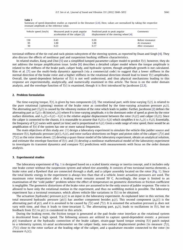
Table 1Summary of speed-dependent studies as reported in the literature [2,4]. Here, values are normalized by taking the respective

resonant amplitude as the reference value.

Vehicle speed (km/h) Measured peak to peak angular

acceleration of the caliper [2]

Predicted peak to peak angular

displacement of the steering wheel [4]

Comments

130 0.43 0.20 Before resonance

95 1.00 1.00 At resonance

50 0.23 0.17 After resonance

O.T. Sen et al. / Journal of Sound and Vibration 331 (2012) 5040–5053 5041

torsional stiffness of the tie-rod and rack-pinion subsystem of the steering system, as reported by Duan and Singh [4]. Theyalso discuss the effects of nonlinear pad and suspension bushing stiffness characteristics.

In related studies, Kang and Choi [5] use a simplified lumped parameter caliper model to predict T(t); however, they donot address the torque amplification issue. Leslie [6] describes a detailed caliper model where the torque amplitude isrelated to the stiffness of the brake pads, caliper body, and hydraulic system, though amplitude growth is not calculated.Kim et al. [7] use the multi-body dynamics approach (via a commercial code) to suggest that a lower stiffness in thenormal direction of the brake rotor and a higher stiffness in the rotational direction should lead to lower T(t) amplitudes.Overall, the speed-dependent behavior of T(t) is not well understood, and thus physical mechanisms leading to thisresponse are experimentally, analytically, and numerically examined in this article. The focus is on the order domainanalysis, and the envelope function of T(t) is examined, though it is first introduced by Jacobsson [2,3].

2. Problem formulation

The time-varying torque, T(t), is given by two components [2]. The rotational part, with time-varying Tr(t), is related tothe pure rotational (spinning) motion of the brake rotor as controlled by the time-varying actuation pressure pr(t).The alternating part (Ta(t)) is caused by the vibratory motion of the rotor which leads to judder. Further, Jacobsson [2] defines thealternating part as Ta(t)¼B(t)sin(nd1c(t)) where B is time-varying amplitude, n is the dominant order of speed as given by the rotorsurface distortion, and d1c(t)¼y1(t)�yc(t) is the relative angular displacement between the rotor (y1(t)) and caliper (yc(t)). Sincethe caliper is connected to the chassis, it is reasonable to assume that y1(t)byc(t) which simplifies it to d1c(t)ffiy1(t). Essentially,the frequency of Ta(t) varies with speed (or time) and is proportional to y1(t). Given a wide range of rotor speed, there would be anamplification of T(t) if the system has one or more natural frequencies.

The main objectives of this study are: (1) design a laboratory experiment to simulate the vehicle-like judder source andmeasure T(t), hydraulic pressure (p(t)), y1(t), and rotor surface distortions on finger and piston sides of the caliper (xf(t) andxp(t)) as the rotor slows down; (2) develop a quasi-linear model of the laboratory experiment, obtain an analytical solution,and estimate the envelope function of T(t); and (3) develop a nonlinear mathematical model of the laboratory experimentto investigate its transient dynamics and compare T(t) predictions with measurements with focus on the order domainanalysis.

3. Experimental studies

The laboratory experiment of Fig. 1 is designed based on a scaled kinetic energy or inertia concept, and it includes onlyone brake corner without the suspension system and wheel-tire assembly. It consists of two torsional inertia elements, abrake rotor and a flywheel that are connected through a shaft, and a caliper assembly located on the rotor (Fig. 1). Sincethe total kinetic energy in the experiment is always less than that of a vehicle, lower actuation pressures are used. Themaximum rotor temperature after a braking event remains around 50 1C. Accordingly, the scope is limited to anexamination of the ‘‘cold judder’’ problem where the effect of temperature on geometric distortions or friction coefficientis negligible. The geometric distortions of the brake rotor are assumed to be the only source of judder response. The rotor isallowed to have only the rotational motion in the experiment, and thus no wobbling motion is possible. The laboratoryexperiment has a torsional resonance, which allows vehicle-like variations in T(t) to be obtained.

The actuation (hydraulic) pressure pr(t) is an input in the laboratory experiment. As explained later in this section, thetotal measured hydraulic pressure (p(t)) has another component besides pr(t). This second component (pa(t)) is thealternating part of p(t), and it is assumed to be caused by xf(t) and xp(t). It is assumed the actuation pressure pr does notvary with time, and thus it leads to time-invariant Tr. The alternating part, pa(t), leads to oscillations in T(t), but nofeedback from T(t) to p(t) is considered in this article.

During the braking event, the friction torque is generated at the pad–brake rotor interface as the rotational systemis decelerated from a high speed. The following sensors are utilized to capture speed-dependent events: a pressurep(t) transducer at the hydraulic connection of the brake caliper, strain-gage based torque sensing T(t) patch outputto a telemetry system, tri-axial accelerometer on the caliper body, non-contact displacement probes (to measure xf(t),xp(t)) close to the rotor surface at the leading edge of the caliper, and a quadrature encoder connected to the rotor (tomeasure y1(t)).

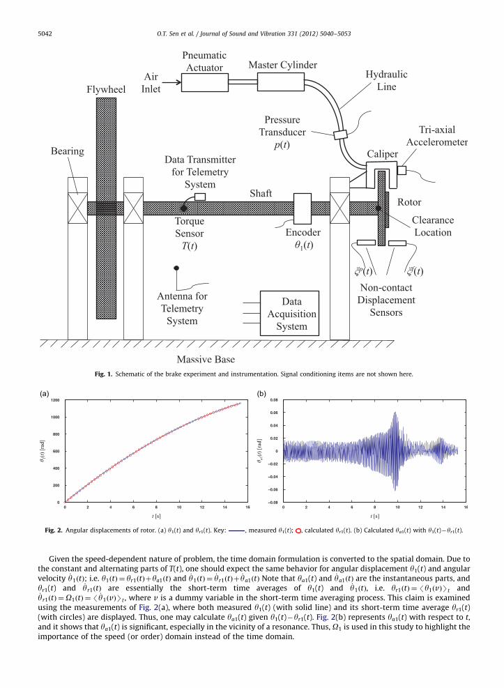
Fig. 1. Schematic of the brake experiment and instrumentation. Signal conditioning items are not shown here.

Fig. 2. Angular displacements of rotor. (a) y1(t) and yr1(t). Key: , measured y1(t); , calculated yr1(t). (b) Calculated ya1(t) with y1(t)�yr1(t).

O.T. Sen et al. / Journal of Sound and Vibration 331 (2012) 5040–50535042

Given the speed-dependent nature of problem, the time domain formulation is converted to the spatial domain. Due tothe constant and alternating parts of T(t), one should expect the same behavior for angular displacement y1(t) and angularvelocity _y1ðtÞ; i.e. y1ðtÞ ¼ yr1ðtÞþya1ðtÞ and _y1ðtÞ ¼ _yr1ðtÞþ _ya1ðtÞ Note that ya1(t) and _ya1ðtÞ are the instantaneous parts, andyr1(t) and _yr1ðtÞ are essentially the short-term time averages of y1(t) and _y1ðtÞ, i.e. yr1ðtÞ ¼/y1ðvÞSt and_yr1ðtÞ ¼O1ðtÞ ¼/ _y1ðvÞSt , where v is a dummy variable in the short-term time averaging process. This claim is examinedusing the measurements of Fig. 2(a), where both measured y1(t) (with solid line) and its short-term time average yr1(t)(with circles) are displayed. Thus, one may calculate ya1(t) given y1(t)�yr1(t). Fig. 2(b) represents ya1(t) with respect to t,and it shows that ya1(t) is significant, especially in the vicinity of a resonance. Thus, O1 is used in this study to highlight theimportance of the speed (or order) domain instead of the time domain.

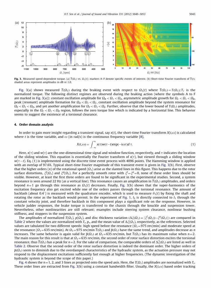
Fig. 3. Measured speed-dependent torque. (a) TðO1Þ vs. O1(t); markers A–F denote specific events of interest. (b) Short-time Fourier transform of TðtÞ;

shaded areas represent amplitudes in dB re 1.0.


Fig. 3(a) shows measured TðO1Þ during the braking event with respect to O1(t) where TðO1Þ ¼ TðO1Þ=Tr is thenormalized torque. The following distinct regimes are observed during the braking action (where the symbols A to Fare marked in Fig. 3(a)): constant oscillation amplitude for OBoO1oOA, asymmetric amplitude growth for OC oO1oOB,peak (resonant) amplitude formation for ODoO1oOC , constant oscillation amplitude beyond the system resonance forOEoO1oOD, and yet another amplification for OFoO1oOE. Further, observe that the lower bound of TðO1Þ amplitudes,especially in the OC oO1oOB region, follows the zero torque line which is indicated by a horizontal line. This behaviorseems to suggest the existence of a torsional clearance.

4. Order domain analysis

In order to gain more insight regarding a transient signal, say x(t), the short-time Fourier transform X(t,o) is calculatedwhere t is the time variable, and o (in rad/s) is the continuous frequency variable [8].

Xðt,oÞ ¼Z 1�1

xðtÞwðt�tÞexpð�iotÞd t: (1)

Here, x(t) and w(t) are the one-dimensional time signal and window function, respectively, and t indicates the locationof the sliding window. This equation is essentially the Fourier transform of x(t), but viewed through a sliding windoww(t�t). Eq. (1) is implemented using the discrete time event process with 4096 points. The Hamming window is appliedwith an overlap of 97.6%. Typical short-time Fourier magnitude of this transient event is given in Fig. 3(b). First, observethat the higher orders (n) of the rotational speed (O1) arise as the slanted lines in this figure. This happens due to the rotorsurface distortions, xf(O1) and xp(O1). For a perfectly smooth rotor with xf

¼xp¼0, none of these order lines should be

visible. However, at least the first three orders are found to be significant in the experimental studies. Second, a systemresonance is seen around 22 Hz (as a vertical line). This resonance causes an amplification in TðO1Þ amplitudes, and ordersbeyond n¼1 go through this resonance as O1(t) decreases. Finally, Fig. 3(b) shows that the super-harmonics of theexcitation frequency also get excited while one of the orders passes through the torsional resonance. The amount ofbacklash (about 0.41) is measured with the quadrature encoder, which is used to measure y1(t) by fixing the shaft androtating the rotor as the backlash would permit. In the experiment of Fig. 1, I2 is directly connected to I1 through theconstant velocity joint, and therefore backlash in this component plays a significant role on the response. However, invehicle judder responses, the brake torque is transferred to the chassis through the knuckle and suspension tower.Nevertheless, other nonlinearities are still relevant; examples include steering system clearance, nonlinear bushingstiffness, and stoppers in the suspension system.

The amplitudes of normalized T(O1), p(O1), and disc thickness variation ðDxðO1Þ ¼ 9xfðO1ÞÞ�x

pðO1Þ9Þ are compared in

Table 2 where the values are normalized with Tr, pr, and the mean value of Dx(O1), respectively, as the references. Selectedvalues are tabulated for two different speeds: high speed before the resonance (O1¼975 rev/min) and moderate speed atthe resonance (O1¼635 rev/min). At O1¼975 rev/min TðO1Þ and pðO1Þ have the same trend, and amplitudes decrease as n

increases. The same behavior is again valid for pðO1Þ at O1¼635 rev/min, but TðO1Þ has its maximum value when n¼2.The main reason for this result is that at O1¼635 rev/min, the second order of rotor surface distortion excites the torsionalresonance, thus TðO1Þ has a peak for n¼2. For the sake of comparison, the comparable orders of DxðO1Þ are listed as well inTable 2. Observe that the second order of the rotor surface distortion is indeed the dominant order. The higher orders ofpðO1Þ seem to diminish due to the overdamped characteristics of the hydraulic system, as the actuation pressure may notrespond to the displacement excitations sufficiently fast enough at higher frequencies. (The dynamic investigation of thehydraulic system is beyond the scope of this paper.)

Fig. 4 shows the n¼1, 2, and 3 lines as projected onto the speed axis. Here, the T(O1) amplitudes are normalized with Tr.These order lines are extracted from Fig. 3(b) using a constant bandwidth filter. Usually, the X(t,o) based order tracking

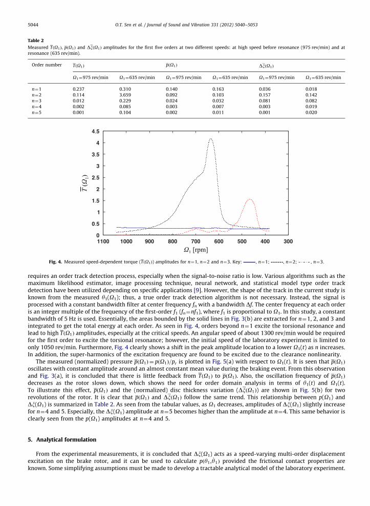
Table 2

Measured TðO1Þ, pðO1Þ and DxðO1Þ amplitudes for the first five orders at two different speeds: at high speed before resonance (975 rev/min) and at

resonance (635 rev/min).

Order number TðO1Þ pðO1Þ DxðO1Þ

O1¼975 rev/min O1¼635 rev/min O1¼975 rev/min O1¼635 rev/min O1¼975 rev/min O1¼635 rev/min

n¼1 0.237 0.310 0.140 0.163 0.036 0.018

n¼2 0.114 3.659 0.092 0.103 0.157 0.142

n¼3 0.012 0.229 0.024 0.032 0.081 0.082

n¼4 0.002 0.085 0.003 0.007 0.003 0.019

n¼5 0.001 0.104 0.002 0.011 0.001 0.020

Fig. 4. Measured speed-dependent torque (TðO1Þ) amplitudes for n¼1, n¼2 and n¼3. Key: , n¼1; , n¼2; , n¼3.


requires an order track detection process, especially when the signal-to-noise ratio is low. Various algorithms such as themaximum likelihood estimator, image processing technique, neural network, and statistical model type order trackdetection have been utilized depending on specific applications [9]. However, the shape of the track in the current study isknown from the measured y1(O1); thus, a true order track detection algorithm is not necessary. Instead, the signal isprocessed with a constant bandwidth filter at center frequency fn with a bandwidth Df. The center frequency at each orderis an integer multiple of the frequency of the first-order f1 (fn¼nf1), where f1 is proportional to O1. In this study, a constantbandwidth of 5 Hz is used. Essentially, the areas bounded by the solid lines in Fig. 3(b) are extracted for n¼1, 2, and 3 andintegrated to get the total energy at each order. As seen in Fig. 4, orders beyond n¼1 excite the torsional resonance andlead to high TðO1Þ amplitudes, especially at the critical speeds. An angular speed of about 1300 rev/min would be requiredfor the first order to excite the torsional resonance; however, the initial speed of the laboratory experiment is limited toonly 1050 rev/min. Furthermore, Fig. 4 clearly shows a shift in the peak amplitude location to a lower O1(t) as n increases.In addition, the super-harmonics of the excitation frequency are found to be excited due to the clearance nonlinearity.

The measured (normalized) pressure pðO1Þ ¼ pðO1Þ=pr is plotted in Fig. 5(a) with respect to O1(t). It is seen that pðO1Þ

oscillates with constant amplitude around an almost constant mean value during the braking event. From this observationand Fig. 3(a), it is concluded that there is little feedback from TðO1Þ to pðO1Þ. Also, the oscillation frequency of pðO1Þ

decreases as the rotor slows down, which shows the need for order domain analysis in terms of y1(t) and O1(t).To illustrate this effect, pðO1Þ and the (normalized) disc thickness variation (DxðO1Þ) are shown in Fig. 5(b) for tworevolutions of the rotor. It is clear that pðO1Þ and DxðO1Þ follow the same trend. This relationship between p(O1) andDx(O1) is summarized in Table 2. As seen from the tabular values, as O1 decreases, amplitudes of Dx(O1) slightly increasefor n¼4 and 5. Especially, the Dx(O1) amplitude at n¼5 becomes higher than the amplitude at n¼4. This same behavior isclearly seen from the p(O1) amplitudes at n¼4 and 5.

5. Analytical formulation

From the experimental measurements, it is concluded that Dx(O1) acts as a speed-varying multi-order displacementexcitation on the brake rotor, and it can be used to calculate pðy1, _y1Þ provided the frictional contact properties areknown. Some simplifying assumptions must be made to develop a tractable analytical model of the laboratory experiment.

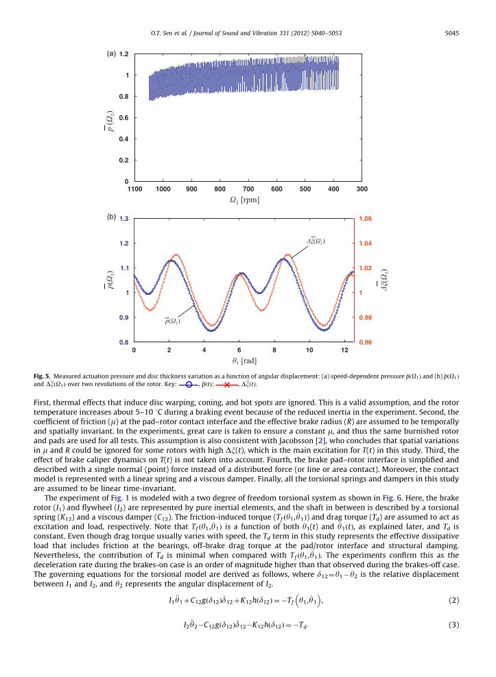
Fig. 5. Measured actuation pressure and disc thickness variation as a function of angular displacement: (a) speed-dependent pressure pðO1Þ and (b) pðO1Þ

and DxðO1Þ over two revolutions of the rotor. Key: , pðtÞ; , DxðtÞ.


First, thermal effects that induce disc warping, coning, and hot spots are ignored. This is a valid assumption, and the rotortemperature increases about 5–10 1C during a braking event because of the reduced inertia in the experiment. Second, thecoefficient of friction (m) at the pad–rotor contact interface and the effective brake radius (R) are assumed to be temporallyand spatially invariant. In the experiments, great care is taken to ensure a constant m, and thus the same burnished rotorand pads are used for all tests. This assumption is also consistent with Jacobsson [2], who concludes that spatial variationsin m and R could be ignored for some rotors with high Dx(t), which is the main excitation for T(t) in this study. Third, theeffect of brake caliper dynamics on T(t) is not taken into account. Fourth, the brake pad–rotor interface is simplified anddescribed with a single normal (point) force instead of a distributed force (or line or area contact). Moreover, the contactmodel is represented with a linear spring and a viscous damper. Finally, all the torsional springs and dampers in this studyare assumed to be linear time-invariant.

The experiment of Fig. 1 is modeled with a two degree of freedom torsional system as shown in Fig. 6. Here, the brakerotor (I1) and flywheel (I2) are represented by pure inertial elements, and the shaft in between is described by a torsionalspring (K12) and a viscous damper (C12). The friction-induced torque (Tf ðy1, _y1Þ) and drag torque (Td) are assumed to act asexcitation and load, respectively. Note that Tf ðy1, _y1Þ is a function of both y1(t) and _y1ðtÞ, as explained later, and Td isconstant. Even though drag torque usually varies with speed, the Td term in this study represents the effective dissipativeload that includes friction at the bearings, off-brake drag torque at the pad/rotor interface and structural damping.Nevertheless, the contribution of Td is minimal when compared with Tf ðy1, _y1Þ. The experiments confirm this as thedeceleration rate during the brakes-on case is an order of magnitude higher than that observed during the brakes-off case.The governing equations for the torsional model are derived as follows, where d12¼y1�y2 is the relative displacementbetween I1 and I2, and y2 represents the angular displacement of I2.

I1€y1þC12g d12ð Þ _d12þK12h d12ð Þ ¼ �Tf y1, _y1

� �, (2)

I2€y2�C12g d12ð Þ _d12�K12h d12ð Þ ¼�Td: (3)

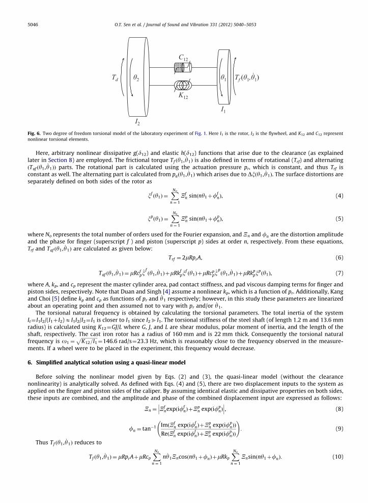
Fig. 6. Two degree of freedom torsional model of the laboratory experiment of Fig. 1. Here I1 is the rotor, I2 is the flywheel, and K12 and C12 represent

nonlinear torsional elements.


Here, arbitrary nonlinear dissipative g(d12) and elastic h(d12) functions that arise due to the clearance (as explainedlater in Section 8) are employed. The frictional torque Tf ðy1, _y1Þ is also defined in terms of rotational (Trf) and alternatingðTaf ðy1, _y1ÞÞ parts. The rotational part is calculated using the actuation pressure pr, which is constant, and thus Trf isconstant as well. The alternating part is calculated from paðy1, _y1Þ which arises due to Dxðy1, _y1Þ. The surface distortions areseparately defined on both sides of the rotor as

xfðy1Þ ¼

XNo

n ¼ 1

Xfn sinðny1þf

fnÞ, (4)

xpðy1Þ ¼

XNo

n ¼ 1

Xpn sinðny1þf

pnÞ, (5)

where No represents the total number of orders used for the Fourier expansion, and Xn and fn are the distortion amplitudeand the phase for finger (superscript f ) and piston (superscript p) sides at order n, respectively. From these equations,Trf and Taf ðy1, _y1Þ are calculated as given below:

Trf ¼ 2mRprA, (6)

Taf ðy1, _y1Þ ¼ mRcfp_x

fðy1, _y1ÞþmRkf

pxfðy1ÞþmRcp

p_x

pðy1, _y1ÞþmRkp

pxpðy1Þ, (7)

where A, kp, and cp represent the master cylinder area, pad contact stiffness, and pad viscous damping terms for finger andpiston sides, respectively. Note that Duan and Singh [4] assume a nonlinear kp, which is a function of pr. Additionally, Kangand Choi [5] define kp and cp as functions of pr and _y1 respectively; however, in this study these parameters are linearizedabout an operating point and then assumed not to vary with pr and/or _y1.

The torsional natural frequency is obtained by calculating the torsional parameters. The total inertia of the systemIt¼ I1I2/(I1þ I2)E I1I2/I2¼ I1 is closer to I1 since I2b I1. The torsional stiffness of the steel shaft (of length 1.2 m and 13.6 mmradius) is calculated using K12¼GJ/L where G, J, and L are shear modulus, polar moment of inertia, and the length of theshaft, respectively. The cast iron rotor has a radius of 160 mm and is 22 mm thick. Consequently the torsional naturalfrequency is o1 ¼

ffiffiffiffiffiffiffiffiffiffiffiffiffiffiK12=I1

p¼146.6 rad/s¼23.3 Hz, which is reasonably close to the frequency observed in the measure-

ments. If a wheel were to be placed in the experiment, this frequency would decrease.

6. Simplified analytical solution using a quasi-linear model

Before solving the nonlinear model given by Eqs. (2) and (3), the quasi-linear model (without the clearancenonlinearity) is analytically solved. As defined with Eqs. (4) and (5), there are two displacement inputs to the system asapplied on the finger and piston sides of the caliper. By assuming identical elastic and dissipative properties on both sides,these inputs are combined, and the amplitude and phase of the combined displacement input are expressed as follows:

Xn ¼ Xfnexpðiff

nÞþXpn expðifp

nÞ

�� , (8)

fn ¼ tan�1 ImðXfn expðiff

nÞþXpn expðifp

nÞÞ

ReðXfn expðiff

nÞþXpn expðifp

nÞÞ

!: (9)

Thus Tf ðy1, _y1Þ reduces to

Tf ðy1, _y1Þ ¼ mRprAþmRcp

XNo

n ¼ 1

n _y1Xncosðny1þfnÞþmRkp

XNo

n ¼ 1

Xnsinðny1þfnÞ: (10)


By ignoring the clearance nonlinearity in Eqs. (2) and (3), linear system equations are obtained as follows:

I1€y1þC12ð

_y1�_y2ÞþK12ðy1�y2Þ ¼ �Tf ðy1, _y1Þ, (11)

I2€y2þC12ð

_y2�_y1ÞþK12ðy2�y1Þ ¼�Td: (12)

Note that the right hand side of Eq. (11) is defined in terms of the motion variables. To get an explicit expression ofTf ðy1, _y1Þ, it is assumed that y1(t) and y2(t) are composed of mean and alternating parts which are being affected by Trf andTaf ðy1, _y1Þ, respectively. Mathematically they are y1(t)¼yr1(t)þya1(t) and y2(t)¼yr2(t)þya2(t). It is reasonably safe toassume that ya2(t) is negligible since I2b I1. Furthermore, it is observed that the angular deceleration of the system duringthe braking experiment is almost constant, €yr2 ¼�L. Accordingly, _yr2 ¼�LtþO0, and yr2 ¼�Lt2=2þO0tþC0. In theseequations, L, O0, and C0 represent the angular deceleration, initial angular velocity, and initial position of I2, respectively.To find an analytical solution for yr1(t), rewrite Eq. (11) for only the mean part as follows:

I1€yr1þC12

_yr1þK12yr1 ¼�mRprAþC12ð�LtþO0ÞþK12 �L2

t2þO0tþC0

� �: (13)

From Eq. (13), yr1(t) is

yr1ðtÞ ¼�L2

t2þO0tþC0K12þ I1L�mRprA

K12

�I1L�mRprA

K12 exp ðC12=2I1Þt� cos

ffiffiffiffiffiffiffiffiffiffiffiffiffiffiffiffiffiffiffiffiffiffiffiffiffiffiffiffiffiffiffiI1K12�ðC

212=4Þ

qI1

t

0@

1Aþ C12

2ffiffiffiffiffiffiffiffiffiffiffiffiffiffiffiffiffiffiffiffiffiffiffiffiffiffiffiffiffiffiffiI1K12�ðC

212=4Þ

q sin

ffiffiffiffiffiffiffiffiffiffiffiffiffiffiffiffiffiffiffiffiffiffiffiffiffiffiffiffiffiffiffiI1K12�ðC

212=4Þ

qI1

t

0@

1A

0B@

1CA: (14)

Eq. (14) shows that yr1(t) follows yr2(t) with a lag that also has both mean and oscillating parts. The oscillating part isneglected by assuming that I1 and I2 rotate as a rigid body, except that I1 follows I2 with this lag. This is a reasonableassumption since the amplitude of the oscillating part is indeed very small (as shown in the next section), and it decreasesas the time passes due to the exponential function at the denominator. This assumption simplifies yr1(t) to

yr1 tð Þ ¼ �L2

t2þO0tþC0K12þLI1�mRprA

K12: (15)

Assume that only yr1(t) affects Tf ðy1, _y1Þ. By incorporating this assumption into Eq. (10), the following is obtained:

Tf ðtÞ ¼ mRprAþmRcp

XNo

n ¼ 1

nð�LtþO0ÞXn cos �nL2

t2þnO0tþFn

� �þmRkp

XNo

n ¼ 1

Xn sin �nL2

t2þnO0tþFn

� �, (16)

where Fn¼nC0þnLI1/K12�nmRprA/K12þfn is a combined phase value. To calculate ya1(t), Eq. (11) is rewritten in terms ofthe alternating parts and transformed to the Laplace domain (s) with zero initial conditions

Ya1ðsÞ ¼1

I1s2þC12sþK12L �Taf ðtÞ �

: (17)

Since Eq. (17) is a product of two functions in the Laplace domain, a convolution of these functions results in thefollowing time domain expression:

ya1ðtÞ ¼

Z t

0

exp � C12ðt�uÞ2I1

� �sin

ðt�uÞffiffiffiffiffiffiffiffiffiffiffiffiffiffiffiffiffiffiffiffiffiffiI1K12�ðC

212=4Þ

pI1

� �ffiffiffiffiffiffiffiffiffiffiffiffiffiffiffiffiffiffiffiffiffiffiffiffiffiffiffiffiffiffiffiI1K12�ðC

212=4Þ

q �Taf ðuÞ �

du, (18)

where u is a dummy variable. The integral for the damped system, as defined by Eq. (18), includes a product of exponentialand trigonometric functions. It may be solved with some algebraic manipulations. However, for the sake of simplicity, anundamped system is defined by ignoring C12 and cp. (As shown in the next section, cp does not affect the results, but C12 hasa significant effect on T(t).) This assumption simplifies Eq. (18) to

ya1ðtÞ ¼XNo

n ¼ 1

Z t

0

sinððt�uÞo1ÞffiffiffiffiffiffiffiffiffiffiffiffiI1K12

p �mRkpXn sin �nL2

u2þnO0uþFn

� �� du: (19)

Note that the order of the integration and summation is changed in Eq. (19). Eq. (19) is written by using thetrigonometric identities as

ya1ðtÞ ¼�mRkp

2ffiffiffiffiffiffiffiffiffiffiffiffiI1K12

p XNo

n ¼ 1

Xn

Z t

0cos

nL2

u2þð�nO0�o1Þuþðo1t�FnÞ

� �du

þmRkp

2ffiffiffiffiffiffiffiffiffiffiffiffiI1K12

p XNo

n ¼ 1

Xn

Z t

0cos �

nL2

u2þðnO0�o1Þuþðo1tþFnÞ

� �du: (20)


Solutions of the integrals given in Eq. (20) are given by the Fresnel integral operators of cosine (C) and sine (S) typerespectively:

Zcosðax2þ2bxþcÞd x¼

ffiffiffiffiffiffip2a

r cos b2�aca

� �C

ffiffiffiffi2

ap

qðaxþbÞ

� �þsin b2

�aca

� �S

ffiffiffiffi2

ap

qðaxþbÞ

� �8><>:

9>=>;: (21)

These integrals are defined by the error (erf) functions as [10]

CðzÞ ¼ Re1þ i

2erf

ffiffiffiffipp

2ð1�iÞz

� � �, (22)

SðzÞ ¼ Im1þ i

2erf

ffiffiffiffipp

2ð1�iÞz

� � �: (23)

By using Eqs. (21)–(23) in (20), ya1(t) is obtained as

ya1ðtÞ ¼ ½Y1a1ðtÞ�Y

1a1ð0Þ��½Y

2a1ðtÞ�Y

2a1ð0Þ�, (24)

Y1a1ðtÞ ¼�

mRkpffiffiffiffipp

2ffiffiffiffiffiffiffiffiffiffiffiffiffiffiffiffiI1K12L

p XNo

n ¼ 1

Xnffiffiffinp

cos ðnO0þo1Þ2

2nL �o1tþFn

� �C 1ffiffiffiffiffiffiffi

nLpp ðnLt�nO0�o1Þ

� �þsin ðnO0þo1Þ

2

2nL �o1tþFn

� �S 1ffiffiffiffiffiffiffi

nLpp ðnLt�nO0�o1Þ

� �8><>:

9>=>;, (25)

Y2a1ðtÞ ¼ �

mRkpffiffiffiffipp

2ffiffiffiffiffiffiffiffiffiffiffiffiffiffiffiffiI1K12L

p XNo

n ¼ 1

Xnffiffiffinp

cos ð�nO0þo1Þ2

2nL þo1tþFn

� �C 1ffiffiffiffiffiffiffi

nLpp ðnLt�nO0þo1Þ

� �þsin ð�nO0 þo1Þ

2

2nL þo1tþFn

� �S 1ffiffiffiffiffiffiffi

nLpp ðnLt�nO0þo1Þ

� �8><>:

9>=>;: (26)

The arguments of Fresnel integrals given by Eqs. (25) and (26) represent slow and fast time scales. It is obvious that theslow time scale is related to the envelope function concept as initially described by Jacobsson [2,3]. The most dominantterm in these arguments is nO0. Since the term nLt has the same sign for both arguments, the last term, which is o1,should be checked to determine the fast and slow time scales. Since nO0 and o1 have the same sign for the argument ofEq. (25), this argument should be related to the fast time scale. Thus, the argument of Eq. (26) is used to propose a refinedenvelope function:

EðtÞ ¼XNo

n ¼ 1

ffiffiffiffiffiffiffiffiffiffiffiffiffiffiffiffiffiffiffiffiffiffiffiffiffiffiffiffiffiffiffiffiffiffiffiffiffiffiffiffiffiffiffiffiffiffiffiffiffiffiffiffiffiffiffiffiffiffiffiffiffiffiffiffiffiffiffiffiffiffiffiffiffiffiffiffiffiffiffiffiffiffiffiffiffiffiffiffiffi½CðrnðtÞÞ�Cðrnð0ÞÞ�

2þ½SðrnðtÞÞ�Sðrnð0ÞÞ�2

q, (27)

rnðtÞ ¼1ffiffiffiffiffiffiffiffiffiffi

nLpp ðnLt�nO0þo1Þ: (28)

Compare this with Jacobsson’s expression [2], where the angular displacement of the caliper is defined as

yc(t)¼aS(t)sin(ny1(t))þaC(t) cos(ny1(t)), where aS and aC are time varying functions with a slow time scale compared to

the sin(ny1(t)) and cos(ny1(t)) terms. Hence, the envelope function of yc(t) is obtained as EðtÞ ¼ffiffiffiffiffiffiffiffiffiffiffiffiffiffiffiffiffiffiffiffiffiffiffiffiffiffiffiffiasðtÞ

2þacðtÞ

2q

. In the

current article, aS and aC are numerically determined. In yet another paper, Jacobsson [3] uses a similar method and

obtains the envelope function as EðtÞ ¼ffiffiffiffiffiffiffiffiffiffiffiffiffiffiffiffiffiffiffiffiffiffiffiffiffiffiffiffiffiffiffiY1ðtÞ

2þY2ðtÞ

2q

where Y1(t)¼Re(V1(t)) and Y2(t)¼ Im(V1(t)). Here, Re and Im denote

real and imaginary parts. In Jacobsson’s paper [3], the expression for V1(t) is similar to Eq. (26) as derived above, exceptthat a multi-order surface distortion profile is assumed in our study. The approach adopted in the current paper differsfrom an older study where Lewis [11] had approximated the envelope of the transient response for a single degree offreedom system in the vicinity of the resonance by using contour integration procedure for selected cases.

7. Comparison of analytical and numerical solutions

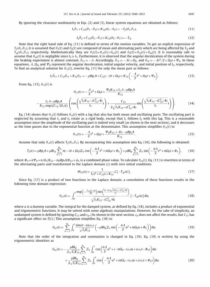
The analytical expression of Section 6 is verified by using the numerical solution of the quasi-linear model. Fig. 7compares the analytical and numerical predictions of normalized torque TðtÞ. First, the same trend is seen for bothmethods: constant TðtÞ amplitude for OBoO1oOA; peak amplitude formation for OC oO1oOB; yet another constant TðtÞ

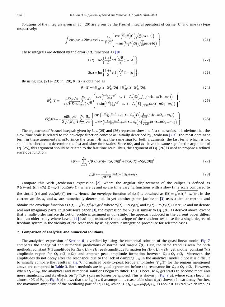
amplitude region for OEoO1oOC; and another peak amplitude formation between OF oO1oOE. Moreover, theamplitudes do not decay after the resonance, due to the lack of damping C12 in the analytical model. Since it is difficultto visually compare the results in Fig. 7, normalized peak-to-peak torque amplitudes ðTppðtÞÞ for the regions mentionedabove are compared in Table 3. Both methods are in good agreement before the resonance for OBoO1oOA. However,when O1oOB, the analytical and numerical solutions begin to differ. This is because ya1(t) starts to become more andmore significant, and its effects on Tf ðy1, _y1Þ can no longer be ignored. This is shown in Fig. 8(a), where _ya1ðtÞ becomesalmost 40% of _yr1ðtÞ. Fig. 8(b) shows that the _ya2ðtÞ ¼ 0 assumption is reasonable since _y2ðtÞ shows a linear decay. Further,the maximum amplitude of the oscillating part of Eq. (14), which is LI1/K12�mRprA/K12, is about 0.008 rad, which implies

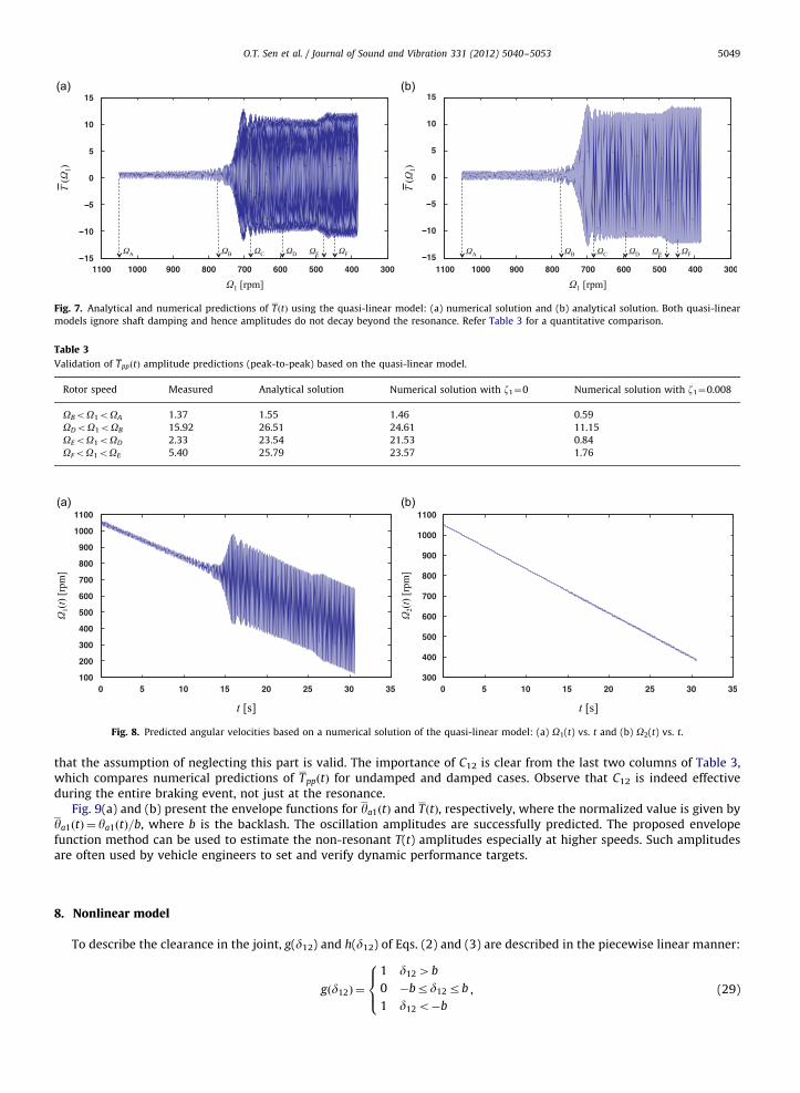
Fig. 7. Analytical and numerical predictions of TðtÞ using the quasi-linear model: (a) numerical solution and (b) analytical solution. Both quasi-linear

models ignore shaft damping and hence amplitudes do not decay beyond the resonance. Refer Table 3 for a quantitative comparison.

Table 3

Validation of TppðtÞ amplitude predictions (peak-to-peak) based on the quasi-linear model.

Rotor speed Measured Analytical solution Numerical solution with z1¼0 Numerical solution with z1¼0.008

OBoO1oOA 1.37 1.55 1.46 0.59

ODoO1oOB 15.92 26.51 24.61 11.15

OEoO1oOD 2.33 23.54 21.53 0.84

OFoO1oOE 5.40 25.79 23.57 1.76

Fig. 8. Predicted angular velocities based on a numerical solution of the quasi-linear model: (a) O1(t) vs. t and (b) O2(t) vs. t.


that the assumption of neglecting this part is valid. The importance of C12 is clear from the last two columns of Table 3,which compares numerical predictions of TppðtÞ for undamped and damped cases. Observe that C12 is indeed effectiveduring the entire braking event, not just at the resonance.

Fig. 9(a) and (b) present the envelope functions for ya1ðtÞ and TðtÞ, respectively, where the normalized value is given byya1ðtÞ ¼ ya1ðtÞ=b, where b is the backlash. The oscillation amplitudes are successfully predicted. The proposed envelopefunction method can be used to estimate the non-resonant T(t) amplitudes especially at higher speeds. Such amplitudesare often used by vehicle engineers to set and verify dynamic performance targets.

8. Nonlinear model

To describe the clearance in the joint, g(d12) and h(d12) of Eqs. (2) and (3) are described in the piecewise linear manner:

gðd12Þ ¼

1 d124b

0 �brd12rb

1 d12o�b

,

8><>: (29)

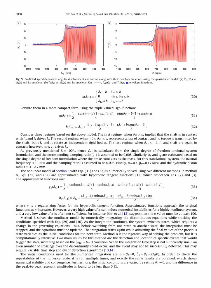
Fig. 9. Predicted speed-dependent angular displacement and torque along with their envelope functions using the quasi-linear model: (a) ya1ðO1Þ vs.

O1(t) and its envelope; (b) TðO1Þ vs. O1(t) and its envelope. Key: , ya1ðO1Þ and TðO1Þ; , envelope functions.


h d12ð Þ ¼

d12�b d124b

0 �brd12rb

d12þb d12o�b

:

8><>: (30)

Rewrite them in a more compact form using the triple valued ‘sgn’ function:

gðd12Þ ¼1

2þ

sgnðd12�bÞð1þsgnðd12ÞÞ

4�

sgnðd12þbÞð1�sgnðd12ÞÞ

4, (31)

hðd12Þ ¼ d12þðd12�bÞsgnðd12�bÞ

2�ðd12þbÞsgnðd12þbÞ

2: (32)

Consider three regimes based on the above model. The first regime, when d124b, implies that the shaft is in contactwith I1, and I1 drives I2. The second regime, when �brd12rb, represents a loss of contact, and no torque is transmitted bythe shaft; both I1 and I2 rotate as independent rigid bodies. The last regime, when d12o�b, I1 and shaft are again incontact; however, now I2 drives I1.

As previously mentioned I2ffi100I1, hence C12 is calculated from the single degree of freedom torsional systemformulation, and the corresponding damping ratio (z1) is assumed to be 0.008. Similarly, kp and cp are estimated based onthe single degree of freedom formulation where the brake rotor acts as the mass. For this translational system, the naturalfrequency is 110 Hz and the damping ratio is assumed to be 0.006. Finally, m¼0.4, pr¼0.17 MPa, and the hydraulic pistonradius s is 12.7 mm.

The nonlinear model of Section 5 with Eqs. (31) and (32) is numerically solved using two different methods. In methodA, Eqs. (31) and (32) are approximated with hyperbolic tangent functions [12] which smoothen Eqs. (2) and (3).The approximated functions are:

g1ðd12Þffi1

2þ

tanhðsðd12�bÞÞð1þtanhðsd12ÞÞ

4�

tanhðsðd12þbÞÞð1�tanhðsd12ÞÞ

4, (33)

h1 d12ð Þffid12þd12�bð Þtanh s d12�bð Þð Þ

2�

d12þbð Þtanh s d12þbð Þð Þ

2, (34)

where s is a regularizing factor for the hyperbolic tangent function. Approximated functions approach the originalfunctions as s increases. However, a very high value of s can induce numerical instabilities for a highly nonlinear system,and a very low value of s is often not sufficient. For instance, Kim et al. [12] suggest that the s value must be at least 100.

Method B solves the nonlinear model by numerically integrating the discontinuous equations while tracking theconditions specified with Eqs. (29) and (30). As the integration continues, the system switches states, which requires achange in the governing equations. Thus, before switching from one state to another state, the integration must bestopped, and the equations must be updated. The integration starts again while admitting the final values of the previousstate variables as the initial conditions for the next state. Method B is the rigorous way of solving the problem, but it iscomputationally intensive. Two main issues for this method are the detection and location of specific events that wouldtrigger the state switching based on the 9d129�b¼0 condition. When the integration time step is not sufficiently small, aneven number of crossings over the discontinuity could occur, and the event may not be successfully detected. This mayrequire variable time step and event detection algorithms [13,14].

The initial conditions used for the numerical integration are y1¼y2¼0, _y1 ¼_y2 ¼O1ð0Þ. In order to check the

repeatability of the numerical code, it is run multiple times, and exactly the same results are obtained, which showsnumerical stability and convergence. Furthermore, the initial conditions are varied by setting _y1 ¼ 0, and the difference inthe peak-to-peak resonant amplitudes is found to be less than 0.1%.


9. Experimental validation

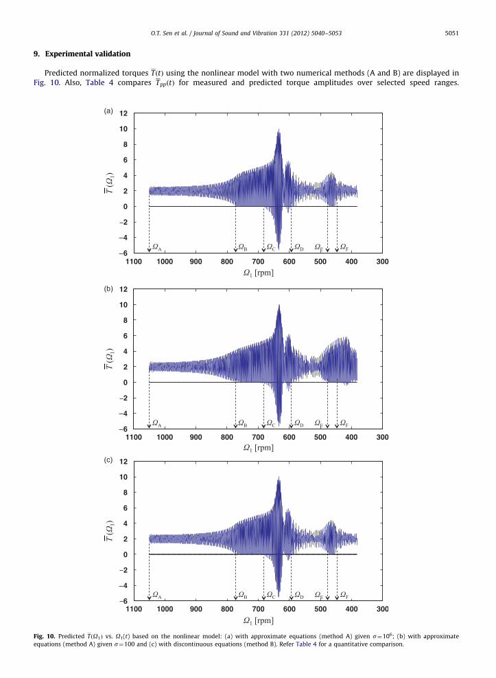
Predicted normalized torques TðtÞ using the nonlinear model with two numerical methods (A and B) are displayed inFig. 10. Also, Table 4 compares TppðtÞ for measured and predicted torque amplitudes over selected speed ranges.

Fig. 10. Predicted TðO1Þ vs. O1(t) based on the nonlinear model: (a) with approximate equations (method A) given s¼106; (b) with approximate

equations (method A) given s¼100 and (c) with discontinuous equations (method B). Refer Table 4 for a quantitative comparison.

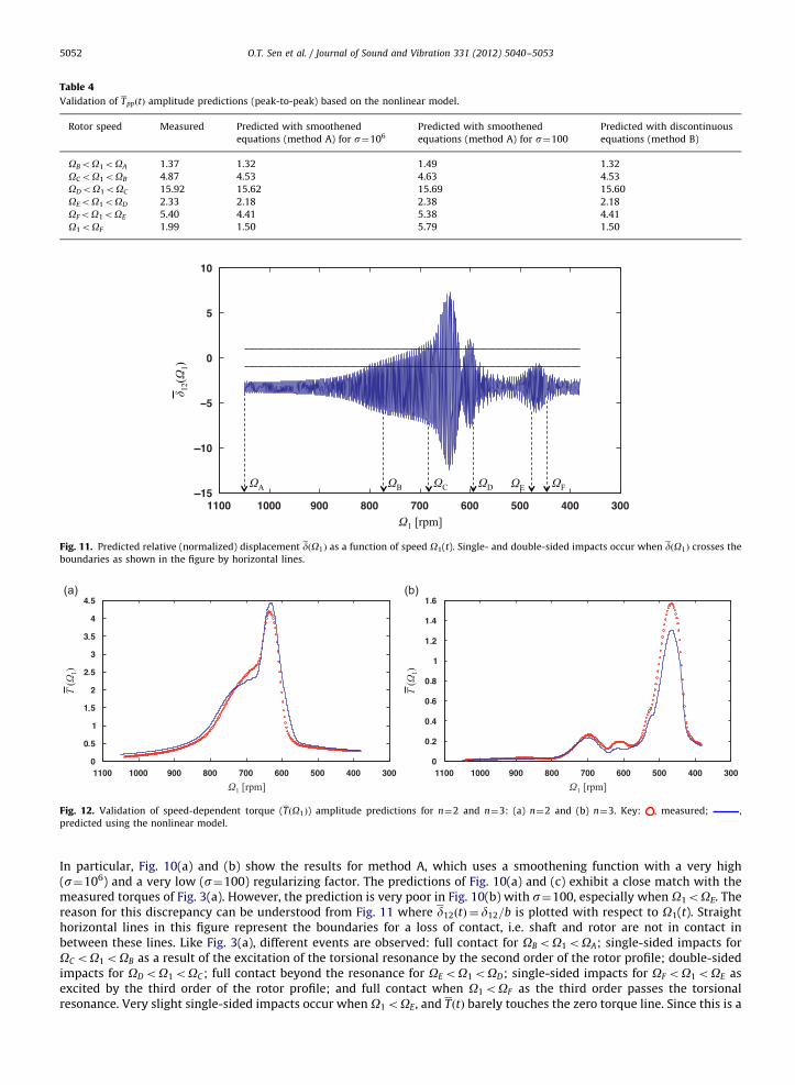
Table 4

Validation of TppðtÞ amplitude predictions (peak-to-peak) based on the nonlinear model.

Rotor speed Measured Predicted with smoothened

equations (method A) for s¼106

Predicted with smoothened

equations (method A) for s¼100

Predicted with discontinuous

equations (method B)

OBoO1oOA 1.37 1.32 1.49 1.32

OCoO1oOB 4.87 4.53 4.63 4.53

ODoO1oOC 15.92 15.62 15.69 15.60

OEoO1oOD 2.33 2.18 2.38 2.18

OFoO1oOE 5.40 4.41 5.38 4.41

O1oOF 1.99 1.50 5.79 1.50

Fig. 11. Predicted relative (normalized) displacement dðO1Þ as a function of speed O1(t). Single- and double-sided impacts occur when dðO1Þ crosses the

boundaries as shown in the figure by horizontal lines.

Fig. 12. Validation of speed-dependent torque (TðO1Þ) amplitude predictions for n¼2 and n¼3: (a) n¼2 and (b) n¼3. Key: , measured; ,

predicted using the nonlinear model.


In particular, Fig. 10(a) and (b) show the results for method A, which uses a smoothening function with a very high(s¼106) and a very low (s¼100) regularizing factor. The predictions of Fig. 10(a) and (c) exhibit a close match with themeasured torques of Fig. 3(a). However, the prediction is very poor in Fig. 10(b) with s¼100, especially when O1oOE. Thereason for this discrepancy can be understood from Fig. 11 where d12ðtÞ ¼ d12=b is plotted with respect to O1(t). Straighthorizontal lines in this figure represent the boundaries for a loss of contact, i.e. shaft and rotor are not in contact inbetween these lines. Like Fig. 3(a), different events are observed: full contact for OBoO1oOA; single-sided impacts forOC oO1oOB as a result of the excitation of the torsional resonance by the second order of the rotor profile; double-sidedimpacts for ODoO1oOC; full contact beyond the resonance for OEoO1oOD; single-sided impacts for OF oO1oOE asexcited by the third order of the rotor profile; and full contact when O1oOF as the third order passes the torsionalresonance. Very slight single-sided impacts occur when O1oOE, and TðtÞ barely touches the zero torque line. Since this is a


transition line between two states, the smoothening approximation is crucial. In the s¼100 case, g1(d12) is under-approximated, which results in a smaller dissipative force. Thus, the impacts do not decay for this particular value of s.

To further validate numerical method B (which uses discontinuous equations), its results are compared withmeasurements in the order domain with the technique described in Section 4. Fig. 12(a) and (b) compare the amplitudesof measured and predicted TðtÞ for n¼2 and n¼3 respectively. Again, a close match between measurements andpredictions validates the nonlinear model.

10. Conclusion

The speed-dependent response of a brake corner has been investigated in this article using experimental, analytical,and numerical approaches. First, a new laboratory experiment has been constructed to simulate vehicle-like judderbehavior. Measurements exhibit a good correlation between p(t) and Dx(t), which suggest that p(t) oscillations areproportionally excited by the surface distortions. In addition, the key regimes during the braking event are successfullyidentified, and their source mechanisms are explained. The order analysis procedures are developed, which clearly showthat at least the first three orders of the rotor surface distortion profile Dx(t) introduce fluctuations in p(t) and T(t). Second,an improved closed form analytical solution of the quasi-linear model has been obtained, and this solution agrees wellwith the numerical solution, especially at higher speeds. Further, the analytical solution is used to obtain the envelopefunction of T(t). The proposed analytical solution and envelope function can be used to set non-resonant T(t) amplitudetargets during product development. Third, a nonlinear model (with clearance) of the experiment is developed byextending the quasi-linear model. This model is numerically solved with two different methods and then experimentallyvalidated. The model was validated numerically, and the resonant amplification of T(t) was predicted successfully in thepresence of clearance nonlinearity.

Several contributions emerge over the prior literature [1–4]. The dynamic friction experiment (as introduced in thisarticle) simulates the vehicle judder in a simplified yet controlled manner; the path clearance conceptually duplicates thekey features of many vehicle system nonlinearities. The controlled experiments yield benchmark data in terms of multiple-orders of the rotor surface distortion profile exciting friction-induced torque. New analytical and numerical solutionsprovide much insight into the speed-dependent resonant amplitude growth process. Nevertheless, the study assumes asimplified contact model and ignores the contributions of caliper and hydraulic system on T(t). Also, only the numericalmethods are utilized to solve the clearance nonlinearity problem. Future research efforts should attempt to improve thesystem models, as well as seek semi-analytical solutions [15,16].

Acknowledgement

The authors gratefully acknowledge Honda R&D Americas, Inc. for supporting this research. The following individualsare thanked for their contributions: W. Post, B. Nutwell, S. Ebert, F. Howse, P. Bray, D. Thompson.

References

[1] H. Jacobsson, Aspects of disc brake judder., Proceedings of the Institution of Mechanical Engineers, Part D: Journal of Automobile Engineering 217 (2003)419–430.

[2] H. Jacobsson, Disc brake judder considering instantaneous disc thickness and spatial friction variation., Proceedings of the Institution of MechanicalEngineers, Part D: Journal of Automobile Engineering 217 (2003) 325–341.

[3] H. Jacobsson, Wheel suspension related disc brake judder, ASME 1997 Design Engineering Technical Conferences, Sacramento, CA, USA, September14–17, 1997.

[4] C. Duan, R. Singh, Analysis of the vehicle brake judder problem by employing a simplified source-path-receiver model., Proceedings of the Institutionof Mechanical Engineers, Part D: Journal of Automobile Engineering 225 (2010) 141–149.

[5] J. Kang, S. Choi, Brake dynamometer model predicting brake torque variation due to disc thickness variation., Proceedings of the Institution ofMechanical Engineers, Part D: Journal of Automobile Engineering 221 (2007) 49–55.

[6] A.C. Leslie, Mathematical model of brake caliper to determine brake torque variation associated with disc thickness variation (DTV) input, SAETechnical Paper 2004-01-2777.

[7] S.H. Kim, E.J. Han, S.W. Kang, S.S. Cho, Investigation of influential factors of a brake corner system to reduce brake torque variation, InternationalJournal of Automotive Technology 9 (2) (2008) 233–247.

[8] A.V. Oppenheim, R.W. Schafer, J.R. Buck, Discrete-Time Signal Processing, 2nd Ed. Prentice Hall, Upper Saddle River, New Jersey, 1999.[9] T.A. Lampert, S.E.M. O0Keefe, A survey of spectrogram track detection algorithms, Applied Acoustics 71 (2010) 87–100.

[10] M. Abramowitz, I.A. Stegun, Handbook of Mathematical Functions with Formulas, Graphs, and Mathematical Tables, National Bureau of StandardsApplied Mathematics Series 55, Washington, DC, 1972.

[11] F.M. Lewis, Vibration during acceleration through a critical speed, Transactions of the American Society of Mechanical Engineers 54 (1932) 253–261.[12] T.C. Kim, T.E. Rook, R. Singh, Effect of smoothening functions on the frequency response of an oscillator with clearance non-linearity, Journal of Sound

and Vibration 263 (2003) 665–678.[13] T. Park, P.I. Barton, State event location in differential-algebraic models, ACM Transactions on Modeling and Computer Simulation 6 (2) (1996) 137–165.[14] L.F. Shampine, S. Thompson, Event location for ordinary differential equations, Journal of Computers and Mathematics with Applications 39 (2000)

43–54.[15] T.C. Kim, T.E. Rook, R. Singh, Super- and sub-harmonic response calculations for a torsional system with clearance nonlinearity using the harmonic

balance method, Journal of Sound and Vibration 281 (2005) 965–993.[16] T.C. Kim, T.E. Rook, R. Singh, Effect of nonlinear impact damping on the frequency response of a torsional system with clearance, Journal of Sound and

Vibration 281 (2005) 995–1021.

Documents

Journal of Sound and Vibration - Acoustics and Dynamics ... et al... · in a brake experiment ... Vehicle brake judder is a friction-induced forced vibration problem, and typically