Contents lists available at ScienceDirect

Journal of Sound and Vibration

Journal of Sound and Vibration 374 (2016) 260–278

http://d0022-46

n CorrE-m

journal homepage: www.elsevier.com/locate/jsvi

Transmission and reflection of acoustic and entropy wavesthrough a stator–rotor stage

Michael Bauerheim a, Ignacio Duran b, Thomas Livebardon b, Gaofeng Wang c,Stéphane Moreau c,n, Thierry Poinsot d

a LMFA, Ecole Centrale de Lyon, 36 Avenue Guy de Collongue, 69130 Ecully, Franceb CERFACS, 31057 Toulouse, Francec Université de Sherbrooke, Sherbrooke, QC, Canada J1K2R1d Institut de Mécanique des Fluides de Toulouse, 31400 Toulouse, France

a r t i c l e i n f o

Article history:Received 4 January 2016Received in revised form30 March 2016Accepted 31 March 2016

Handling Editor: Y. Auregan

entropy waves through a stator vane, developed since the seventies, are generally based

Available online 15 April 2016

x.doi.org/10.1016/j.jsv.2016.03.0410X/& 2016 Elsevier Ltd. All rights reserved.

esponding author.ail address: Stephane.Moreau@USherbrooke.

a b s t r a c t

The propagation of acoustic, entropy and vorticity waves through turbine stages is ofsignificant interest in the field of core noise. In particular, entropy spots have been shownto generate significant noise when accelerated through turbine stages: the so-calledindirect combustion noise. Analytical models for the propagation of acoustic, vorticity and

on restrictive assumptions such as low frequency waves. In order to analyze suchassumptions, the theory of Cumpsty and Marble is extended to rotating rows and appliedto a 2D stator–rotor turbine stage. The theoretical transfer functions are then comparedwith numerical predictions from forced compressible Large-Eddy Simulations of a 2Dstator–rotor configuration, using a fluid–fluid coupling strategy with an overset-gridmethod. The comparisons between the analytical model and the simulations are in goodagreement. To improve the analytical predictions, the attenuation due to the entropy spotdeformation through the stator vane or the rotor blade is then included, modeled eitheranalytically or extracted from the mean flow of the simulations. The complete analyticalmodel reveals a good agreement with 2D simulations, which allows the prediction andminimization of both direct and indirect noise at the design-stage without computation.

& 2016 Elsevier Ltd. All rights reserved.

1. Introduction

The International Civil Aviation Organization (ICAO) predicts a significant increase of air traffic, the latter doubling in thenext two decades. Consequently the environmental impact of airplanes will be even more regulated and stricter limitationson noise and pollutant emissions imposed to aircraft manufacturers by ICAO. Since the first investigations by Lighthill [27],the reduction of aircraft noise has been continuously focused on the main aerodynamic sources: jet, fan, turbomachineryand airframe noise. With mainly the constant increase of the by-pass ratio of turboengines, these sources have been sig-nificantly reduced over the last decades. Other sources such as combustion noise have seen their relative influence increaseover the last years not only because of the aforementioned global reduction of engine noise but also because of shorter,more highly loaded turbines that do not shield it as efficiently, and also the development of new low NOx-emission

ca (S. Moreau).

M. Bauerheim et al. / Journal of Sound and Vibration 374 (2016) 260–278 261

combustion chambers such as lean premixed, rich-quench-lean or staged-injection combustion chambers in which largerturbulent fluctuations lead to unsteady heat release and more noise generation.

Marble and Candel [31] and Cumpsty and Marble [9] showed that there are two main mechanisms of combustion noisegeneration that propagate through the turbine stages to the outlet of the engine: the direct and indirect combustion noise.The former is caused by the acoustic waves generated by the unsteady heat release of turbulent combustion. Thismechanism has been studied by Strahle [40,41] and more recently by Ihme and Pitsch [19] for instance. The latter, also calledentropy noise, is caused by the convection of entropy waves, or hot-spots, through turbine stages. When these entropy spotsare accelerated in the turbine rows, they generate acoustic waves, a mechanism which has been studied by Marble andCandel [31], Cumpsty and Marble [9], Bake et al. [3], Leyko et al. [25,26] and Howe [18]. In some cases, depending on theoutlet conditions of the combustion chamber, entropy noise was thought to be larger than direct noise [6,34,35]. Analyti-cally, Leyko et al. [25] showed with a 1D model combustor with a choked nozzle that indirect noise can be one order ofmagnitude larger than direct noise in actual turbo-engines and negligible in existing laboratory experiments. More recently,this noise mechanism was experimentally shown to be relevant in auxiliary power units [42] and helicopter engines [4,28].

Combustion noise is therefore strongly connected with the propagation of acoustic and entropy waves through theturbine stages. In the case of direct noise, the propagation through turbine rows contributes to the noise attenuation whilein the case of the indirect mechanism, noise is produced during the propagation of the entropy wave through an accel-erating flow. Marble and Candel [31] developed a first analytical method to predict the noise generated at the outlet of a 1Dnozzle by acoustic and entropy waves. This analytical solution is based on the compact nozzle assumption, in which thewavelengths of the perturbations are assumed to be much larger than the 1D nozzle dimensions, limiting the results to thevery low frequency range. Jump conditions can then be written between the inlet and the outlet of the compact nozzle forthe mass, total temperature and entropy fluctuations. By comparing with the experimental data of Bake et al. [3], such a 1Danalytical model was validated by Leyko et al. [26] in the case of a supersonic flow, and by Duran et al. [14] in the subsoniccase. The validity of the compact nozzle hypothesis has been investigated numerically [1,22,15], and analytical modeling hasbeen extended for non-compact frequencies [13,16,17,39].

Based on 1D models, several analytical and semi-analytical models have been extended to predict the propagation ofacoustic waves through turbine blades in 2D configurations such as those developed by Muir [32,33] and Kaji and Okazaki[20,21]. Yet, all these models only consider acoustic and vorticity waves, neglecting entropy fluctuations and thereforeindirect noise. To include the additional effect of entropy waves, Cumpsty and Marble [9] extended the aforementioned 1Danalytical model of Marble and Candel [31] to a stator vane in a 2D configuration at midspan accounting for the significanteffect of flow deviation in a turbine, and including vorticity waves through the stator vane. This method was compared byLeyko et al. [24,23] with numerical simulations for the case of a stator vane showing that the compact low-frequency limit ofthe analytical method predicted correctly the transfer functions (both the reflected and transmitted acoustic waves) gen-erated by acoustic and entropy waves. For the case of direct noise, the compact solution was shown to be valid over a widerange of frequencies. For the case of indirect noise however, the entropy wave was shown to be strongly deformed by thepresence of the stator blade. The indirect noise was nevertheless shown to be correctly predicted at low frequencies, whichare dominant in combustion noise.

In this context, the goal of the present study is to extend the previous work of Leyko et al. [24,23] to the propagation ofwaves through a complete realistic turbine stage, containing both a stator and a rotor. The 2D analytical model of Cumpsty andMarble [9] is first explained in Section 2, and then extended to take into account the effect of the rotor blade. This yields acomplete propagation model through a full compact multi-stage turbomachinery termed CHORUS. Detailed numericalunsteady simulations are then performed to obtain reference transfer functions at all frequencies to validate the analyticalresults. The set-up of these simulations is explained in Section 3 and results are discussed in Section 4. A new analyticalindirect noise model is proposed based on a modeled axial velocity profile yielding an analytical formulation of the attenuationof entropy waves through a turbine row, and a parametric study is undertaken. Conclusions are finally drawn in Section 5.

2. Analytical method

The analytical method developed by Cumpsty and Marble [9] to predict the wave propagation through stator blades isfirst recast in matrix form and extended to rotating blades. The model relies on the compact assumption, which considersthat the wavelengths of the perturbations are greater than the axial length of the turbine stages. With this assumption, theacoustic and entropy waves propagate quasi-steadily through the turbine stages, and jump conditions can be simply writtenbetween the inlet and the outlet of each turbine row. A 2D blade-to-blade configuration is considered (any radial variationare omitted), and the flow upstream and downstream of each blade row is assumed steady and uniform (mean speedtriangles at the mean radius R of the meridian plane of the turbine). Fig. 1 shows a sketch of such a configuration: aninfinitely thin blade row behaves as an interface between two regions of uniform flow. w represents the mean relative flow-velocity vector (with module w and an angle θ with the axial direction), and k is the wave vector that provides the pro-pagation direction of the considered wave (similarly with module k and angle ν with the axial direction).

The mean flow is described by four variables: w, θ , the mean pressure p and the mean density of the flow ρ. This meanflow is perturbed by small fluctuations, which can be described by four primitive variables: the entropy perturbation s0, therelative-velocity perturbation w0, the pressure fluctuation p0, and the perturbation of the flow angle θ0.

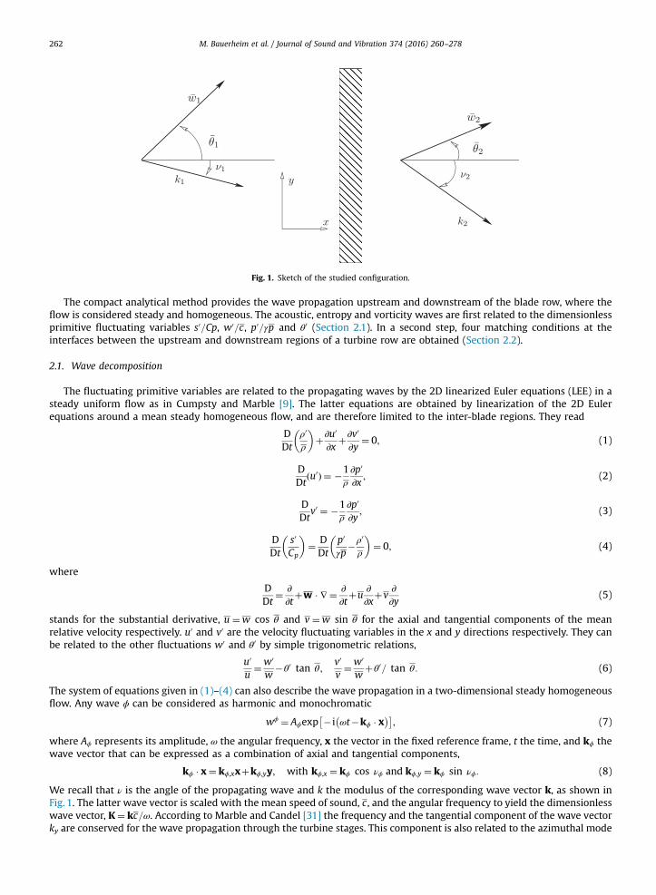
Fig. 1. Sketch of the studied configuration.

M. Bauerheim et al. / Journal of Sound and Vibration 374 (2016) 260–278262

The compact analytical method provides the wave propagation upstream and downstream of the blade row, where theflow is considered steady and homogeneous. The acoustic, entropy and vorticity waves are first related to the dimensionlessprimitive fluctuating variables s0=Cp, w0=c, p0=γp and θ0 (Section 2.1). In a second step, four matching conditions at theinterfaces between the upstream and downstream regions of a turbine row are obtained (Section 2.2).

2.1. Wave decomposition

The fluctuating primitive variables are related to the propagating waves by the 2D linearized Euler equations (LEE) in asteady uniform flow as in Cumpsty and Marble [9]. The latter equations are obtained by linearization of the 2D Eulerequations around a mean steady homogeneous flow, and are therefore limited to the inter-blade regions. They read

DDt

ρ0

ρ

� �þ∂u0

∂xþ∂v0

∂y¼ 0; (1)

DDt

ðu0Þ ¼ �1ρ

∂p0

∂x; (2)

DDt

v0 ¼ �1ρ

∂p0

∂y; (3)

DDt

s0

Cp

� �¼ DDt

p0

γp�ρ0

ρ

� �¼ 0; (4)

where

DDt

¼ ∂∂tþw � ∇¼ ∂

∂tþu

∂∂x

þv∂∂y

(5)

stands for the substantial derivative, u ¼w cos θ and v ¼w sin θ for the axial and tangential components of the meanrelative velocity respectively. u0 and v0 are the velocity fluctuating variables in the x and y directions respectively. They canbe related to the other fluctuations w0 and θ0 by simple trigonometric relations,

u0

u¼w0

w�θ0 tan θ ;

v0

v¼w0

wþθ0= tan θ : (6)

The system of equations given in (1)–(4) can also describe the wave propagation in a two-dimensional steady homogeneousflow. Any wave ϕ can be considered as harmonic and monochromatic

wϕ ¼ Aϕexp � i ωt�kϕ � x� �� �; (7)

where Aϕ represents its amplitude, ω the angular frequency, x the vector in the fixed reference frame, t the time, and kϕ thewave vector that can be expressed as a combination of axial and tangential components,

kϕ � x¼ kϕ;xxþkϕ;yy; with kϕ;x ¼ kϕ cos νϕ and kϕ;y ¼ kϕ sin νϕ: (8)

We recall that ν is the angle of the propagating wave and k the modulus of the corresponding wave vector k, as shown inFig. 1. The latter wave vector is scaled with the mean speed of sound, c, and the angular frequency to yield the dimensionlesswave vector, K¼ kc=ω. According to Marble and Candel [31] the frequency and the tangential component of the wave vectorky are conserved for the wave propagation through the turbine stages. This component is also related to the azimuthal mode

M. Bauerheim et al. / Journal of Sound and Vibration 374 (2016) 260–278 263

order m through kϕ;y ¼m=R. Yet, this is not the case for the dimensionless tangential component Kϕ;y, since the mean speedof sound may vary through the blade rows.

Eqs. (1)–(4) can then be used to relate, for each wave, the wave vector to the angular frequency, the mean Mach numberM ¼w=c, and the flow direction θ .

2.1.1. Entropy waveThe entropy wave, ws ¼ s0=Cp, is defined as

ws ¼ s0

Cp¼ Asexp � i ωt�ks � xð Þ� �

: (9)

The dispersion equation is obtained by combining Eq. (9) with the transport equation of the entropy wave, Eq. (4),

KsM cos νs�θ� ��1¼ 0: (10)

This dispersion equation then yields the axial component of the wave vector, Ks;x, as a function of the tangential component,the angular frequency, and the mean flow Mach number and direction.

By definition, the entropy wave does not yield pressure or velocity perturbations, and the fluctuations of the primitivevariables (s0=Cp, w0=c, p0=γp and θ0) generated by the entropy wave are therefore

s0=Cp

w0=c

p0=γp

θ0

8>>><>>>:

9>>>=>>>;

s

¼

1000

8>>><>>>:

9>>>=>>>;ws: (11)

2.1.2. Vorticity waveThe vorticity wave is defined as the curl of the fluctuating velocity field

ξ0 ¼ ∂v0

∂x�∂u0

∂y: (12)

The transport equation for the vorticity wave can be derived from Eqs. (2) and (3). Differentiating Eq. (2) with respect to yand Eq. (3) with respect to x lead to

∂∂y

DDt

u0ð Þ� �

¼ �1ρ

∂2p0

∂x∂y;

∂∂x

DDt

v0ð Þ� �

¼ �1ρ

∂2p0

∂y∂x: (13)

Subtracting both relations and using Schwarz's theorem, the pressure term can be eliminated, yielding the vorticity equation

DDt

ξ0ð Þ ¼ 0: (14)

As the entropy wave, the vorticity wave can be assumed harmonic and monochromatic,

wv ¼ ξ0

ω¼ Avexp � i ωt�kv � xð Þ� �

: (15)

The dispersion equation of the vorticity wave can be obtained by combining Eq. (14) with Eq. (15), namely

KvM cos νv�θ� ��1¼ 0: (16)

As shown by Chu and Kovasznay [7], no pressure or entropy fluctuations are associated with this wave to first order. Eq. (4)then shows that there are no density fluctuations either. Eq. (1) can be reduced to

∂u0

∂xþ∂v0

∂y¼ 0: (17)

Using Eq. (15) the velocity field can be written as

u0

c¼ � i

ξ0

ω

sin νvð ÞKv

;

v0

c¼ i

ξ0

ω

cos νvð ÞKv

: (18)

These fluctuations are recast in terms of w0 and θ0 using Eq. (6)

w0

c¼ � i

ξ0

ω

sin νv�θ� �Kv

;

M. Bauerheim et al. / Journal of Sound and Vibration 374 (2016) 260–278264

θ0 ¼ iξ0

ω

cos νv�θ� �MKv

: (19)

Using the dimensionless form of the vorticity wave, wv ¼ ξ0=ω, the fluctuations of the primitive variables generated by thiswave are

s0=Cp

w0=c

p0=γp

θ0

8>>><>>>:

9>>>=>>>;

v

¼

0

� isin νv�θ

� �Kv

0

icos νv�θ

� �MKv

8>>>>>>><>>>>>>>:

9>>>>>>>=>>>>>>>;wv: (20)

2.1.3. Acoustic wavesA transport equation for the pressure fluctuations can be obtained by combining Eqs. (1)–(4). Eq. (4) is first used to

eliminate the density term in Eq. (1) and a substantial derivative of the resulting equation is taken,

DDt

� �2" #

p0

γp

� �þ DDt

∂u0

∂x

� �þ DDt

∂v0

∂y

� �¼ 0: (21)

Combining Eq. (21) with the substantial derivative of Eqs. (2) and (3), and knowing that c2 ¼ γp=ρ yields the followingequation for the pressure perturbations:

DDt

� �2

�c2∂2

∂x2þ ∂2

∂y2

� �" #p0

γp

� �¼ 0: (22)

Using the waveform of Eq. (7) for the acoustic waves,

w7 ¼ ρ0

γρ

� �7

¼ A7 exp � i ωt�k7 � xð Þ� �; (23)

the following dispersion equation is obtained:

1�K7M cos ν7 �θ� �� �2�K2

7 ¼ 0; (24)

where K7 is the module of the dimensionless wave vector. As the above acoustic dispersion equation, Eq. (24) has twosolutions, the subscript 7ð Þ stands for the acoustic perturbations propagating downstream (þ , called the transmittedacoustic wave) and upstream (� , called the reflected acoustic wave). This dispersion equation can be rewritten as a functionof the axial and tangential components (K7 ;x and K7 ;y) using Eq. (8),

1�K7 ;xM cos θ�K7 ;yM sin θ� �2�K2

7 ;x�K27 ;y ¼ 0: (25)

When solving for K7 ;x in Eq. (25), K7 ;x can be either a real or a complex value. The real values correspond to acoustic wavespropagating without attenuation through the mean steady flow (cut-on modes), while complex values are evanescentwaves that cannot propagate in the flow (cut-off modes). Solving for cut-on modes in Eq. (25) yields the condition

1�K7 ;yM sin θ� �2� 1�M

2sin 2θ

� K2

7 ;yo0: (26)

For a given mean flow, this relationship, Eq. (26), gives a critical value K7 ;y ¼ ck7 ;y=ω. This shows that for any tangentialacoustic mode k7 ;y there exists a cut-off frequency below which the acoustic waves do not propagate.

Knowing that the wave is isentropic and irrotational [7], the fluctuations of primitive variables generated by the acousticwaves can then be obtained,

s0=Cp

w0=c

p0=γp

θ0

8>>><>>>:

9>>>=>>>;

7

¼

0K7 cos ν7 �θ

� �=½1�K7M cos ν7 �θ

� ��1

K7 sin ν7 �θ� �

=½M 1�K7M cos ν7 �θ� �� ��

8>>>><>>>>:

9>>>>=>>>>;w7 : (27)

M. Bauerheim et al. / Journal of Sound and Vibration 374 (2016) 260–278 265

2.1.4. Transformation matrixFinally, the primitive fluctuating variables can be recast in a matrix form by adding the contribution of each of the four

waves, leading to the following vector relationship:

s0=Cp

w0=c

p0=γp

θ0

8>>><>>>:

9>>>=>>>;¼ M½ � �

ws

wv

wþ

w�

8>>><>>>:

9>>>=>>>;; (28)

where the matrix M½ � is given by the combination of Eqs. (11), (20) and (27),

M½ � ¼

1 0 0 0

0 � i sin νv �θð ÞKv

K þ cos νþ �θð Þ1�K þ M cos νþ � θð Þ� � K � cos ν� �θð Þ

1�K � M cos ν� �θð Þ� �

0 0 1 1

0 i cos νv �θð ÞKvM

K þ sin νþ �θð ÞM 1�K þ M cos νþ � θð Þ� � K � sin ν� �θð Þ

M 1�K � M cos ν� � θð Þ� �

266666664

377777775: (29)

2.2. Jump conditions through the blade row

Once the primitive variables are related to the acoustic, entropy and vorticity waves by Eq. (29) in both upstream anddownstream regions of a blade or vane row, only a relationship between the primitive variables on both sides is needed toclose the problem. Since each blade or vane row is assumed axially compact, the upstream and downstream flow rela-tionship reduces to a jump condition at the interface. Eq. (28) shows that four conditions are required. The latter areobtained using the conservation of mass and energy, and the transport of entropy fluctuations, plus a fourth equation on thetangential component of the flow, obtained through the so-called Kutta condition. As a different form of energy is conservedthrough stationary and rotating rows, the study of the stator vane and of the rotor blade are done separately.

2.2.1. Stator vaneFor the stator vane, the conservation equations of mass and stagnation enthalpy or equivalently stagnation temperature,

and the transport of entropy fluctuations, used by Cumpsty and Marble [9] read,

_m0

_mÞ1¼

_m0

_m

�2;

��T 0t

Tt

� �1¼ T 0

t

Tt

� �2;

s0

Cp

� �1¼ s0

Cp

� �2: (30)

Subscripts 1 and 2 stand for the flow upstream and downstream of the vane row, as shown in Fig. 1. These equations shouldbe rewritten as a function of the primitive variables used previously (s0, p0, w0 and θ0). For the mass and temperaturefluctuations, it yields

_m0

_m

�¼ p0

γpþ 1M

w0

c�θ0 tan θ ;

�(31)

T 0t

Tt

� �¼ 1

1þðγ�1Þ2

M2

γ�1ð Þp0

γpþ s0

Cpþ γ�1ð ÞMw0

c

�: (32)

As mentioned above, Eqs. (30)–(32) should be completed by a fourth condition: Cumpsty and Marble [9] applied the Kuttacondition at the vane outlet. The potential-flow theory indicates that in a steady flow around an airfoil, the effect of viscositycan be accounting for by imposing a condition which removes the trailing-edge pressure or velocity singularity. Thiscondition fixes the pressure jump or the circulation around the airfoil such that the stagnation point is located at thetrailing-edge. For unsteady flows, the Kutta condition used by Cumpsty and Marble [9] states that the flow deviation θ2 isequal to the geometrical angle of the vane trailing edge, and therefore its perturbation should be zero θ02 ¼ 0

� �. Imposing the

correct condition at the trailing edge of the vane row is important to correctly predict the generation of noise at the vanetrailing edge and, in our case, the acoustic transfer functions of the stator vane. Cumpsty and Marble [9] suggest to use amore general unsteady form of the Kutta condition given by

θ02 ¼ βθ01; (33)

where β is either measured when experimental data are available or calculated by semi-empirical methods. In the low-frequency limit used in the present analysis, the Kutta condition with β¼ 0 is generally valid as the flow evolves quasi-steadily.

M. Bauerheim et al. / Journal of Sound and Vibration 374 (2016) 260–278266

Consequently, the jump conditions are obtained by rewriting Eqs. (30) and (33) in a matrix form as a function of theprimitive variables, which read

E1½ � �

s0=Cp

w0=c

p0=γp

θ0

8>>><>>>:

9>>>=>>>;

1

¼ E2½ � �

s0=Cp

w0=c

p0=γp

θ0

8>>><>>>:

9>>>=>>>;

2

; (34)

where E1½ � and E2½ � are defined as

E1½ � ¼

1 0 0 0�1 1

M11 � tan θ1

μ1γ�1 μ1M1 μ1 0

0 0 0 β

2666664

3777775;

E2½ � ¼

1 0 0 0�1 1

M21 � tan θ2

μ2γ�1 μ2M2 μ2 0

0 0 0 1

266664

377775; (35)

and μ¼ 1=½1þðγ�1ÞM2=2�.

2.2.2. Rotor bladeFor a rotor blade, the conservation of stagnation enthalpy (Section 2.2.1) is no longer valid. Instead, the conserved

variable through the blade row is the rothalpy defined as [5,30],

I¼ ht�Uv; (36)

where ht is the specific stagnation enthalpy, U the rotating speed of the blade, and v the tangential component of theabsolute speed (Fig. 2). For the rotating speed, different values are considered at the inlet and outlet of the blade row toaccount for the large expansion of the turbine. The conservation of rothalpy can be derived by combining the energyequation and Euler's equation, and reads

Δht ¼ Δ Uvð Þ ¼U2 � v2�U1 � v1: (37)

Considering small perturbations, a generalized form of the energy equation for rotating blades can then be deduced as,

I01I1

¼ I02I2; (38)

which replaces the second equation in Eq. (30) for the stagnation temperature jump. The rothalpy fluctuation is then written

Fig. 2. Sketch of the flow through a rotor blade. Superscript ðÞr represents the variables in the rotor reference frame.

M. Bauerheim et al. / Journal of Sound and Vibration 374 (2016) 260–278 267

as a function of the primitive variables,

I0

I¼ h0

t�Uv0

ht �Uv¼

h0tht

�Uv

htv0v

1�Uv

ht

: (39)

Knowing that ht ¼ CpTt and defining the parameter ζ as

ζ¼Uv

ht; (40)

Eq. (39) can be recast into,

I0

I¼ 11�ζ

T 0t

Tt�ζ

v0

v

� � �: (41)

As expected, U¼0 implies that ζ¼ 0 (Eq. (40), thus the stagnation temperature jump used for the stator vane is recovered.Moreover, the fluctuating tangential velocity v0=v can be eliminated using Eqs. (6), and (41)) becomes

I0

I¼ 11�ζ

T 0t

Tt�ζ

1M

w0

cþ θ0

tan θ

� � �; (42)

which replaces the stagnation enthalpy conservation in Eqs. (34) and (35). For a rotor, the Kutta condition has to be imposedin its reference frame, yielding

θ0ð Þr2 ¼ β θ0ð Þr1; (43)

where θ0ð Þr is the fluctuation of the relative flow angle. This equation can be recast in the fixed reference frame using thevariables θ0 and w0=w (Fig. 2) and trigonometric relations (Appendix A) as follows:

θ0ð Þr ¼ θ0 1þ Uwr sin θr

� � �þ w0

w

� �Uwr cos θr

� : (44)

2.3. Solution of the propagation equations through a compact multi-stage turbomachinery

The propagation equations through a compact multi-stage turbomachinery are solved in a matrix form by imposing thecorrect waves and boundary conditions at each rotating or stationary row. In the subsonic case, the latter are wþ , ws and wv

at the inlet, and w� at the outlet of the blade or vane row. For instance the waves coming from the combustion chambermust be first decomposed into azimuthal modes related to ky, and into angular frequencies ω. The propagation equations aresolved for each pair (ky, ω) for which the proper dispersion equations can be used to obtain the value of the completedimensionless wave vector K on both sides of a blade or vane row for each wave. Using this information, matrices M and Ecan then be computed on both sides of the blade or vane row.

For a single row, the problem is solved by writing Eq. (34) as a function of the waves using Eq. (28),

E1½ � � M1½ �|fflfflfflfflfflfflffl{zfflfflfflfflfflfflffl}B1½ �

�

ws

wv

wþ

w�

8>>><>>>:

9>>>=>>>;

1

¼ E2½ � � M2½ �|fflfflfflfflfflfflffl{zfflfflfflfflfflfflffl}B2½ �

�

ws

wv

wþ

w�

8>>><>>>:

9>>>=>>>;

2

: (45)

The boundary conditions for each row should only provide the incoming waves. Therefore, Eq. (45) is recast into “scatteringmatrices” Ain½ � and Aout½ � by permuting the fourth column of matrices ½B1� and ½B2� and changing signs. Such a matrixtransformation allows the construction of an equivalent system with imposed waves on the right-hand side of the equa-tions, and the unknowns on the left-hand side only. The “scattered” system replacing Eq. (45) can then be inverted to yieldthe unknown out-coming waves, and reads

Aout½ � �

ws2

wv2

wþ2

w�1

8>>>><>>>>:

9>>>>=>>>>;

¼ Ain½ � �

ws1

wv1

wþ1

w�2

8>>>><>>>>:

9>>>>=>>>>;: (46)

For the case of multiple blade and vane rows of a typical turbomachinery, a phase-shift of the waves through the rowspacing is applied to account for the wave propagation through the entire machine and the interstage gaps. Indeed, even ifeach stator vane or rotor blade can be assumed compact (at least for sufficiently low frequencies), the whole multi-stageturbine is not, because of a cumulative effect. The complete phase shift is therefore recovered by adding a phase shift to eachcomponent, based on an equivalent axial length L. In this study, this length is chosen as the interstage gap corrected withhalf the chord length of adjacent components, namely L¼ Lstator=2þLinterstageþLrotor=2. Since no wave coupling occurs for

M. Bauerheim et al. / Journal of Sound and Vibration 374 (2016) 260–278268

pure wave propagation, a diagonal matrix ½T� is used to impose the phase-shift of the waves, which reads

T½ � ¼

exp iksxL� �

0 0 0

0 exp ikvxL� �

0 0

0 exp ikþx L

� �0

0 0 0 exp ik�x L

� �

2666664

3777775; (47)

Considering Viu and Vi

d the wave vectors upstream and downstream of the i-th blade or vane row respectively, Eq. (45)connects both sides through

Bi1

h i� Vi

u ¼ Bi2

h i� Vi

d: (48)

The downstreamwave vector can be related to the following blade or vane row by Viþ1u ¼ ½Ti� � Vi

d. Combining the successivestages of a turbine, a relationship between the inlet and the outlet waves of the whole turbomachine can be written in amatrix form,

∏Nr �1

i ¼ 1Biþ11

h iTi Bi

2

h i�1 �" #

B11

h i� V1

u ¼ BNr2

h i� VNr

d ; (49)

where Nr is the number of rows. This system of equations can be finally permuted to obtain a “scattered” system similar toEq. (46), which can be inverted to provide the unknown out-coming waves. The resulting analytical tool has been termedCHORUS and included for instance in a complete methodology for predicting combustion noise termed CONOCHAIN [29].

Even though the combination of several blade and vane rows leads to a transfer function which is frequency dependentthrough the wave propagation modeled by Eq. (47), the compact assumption for each individual row still limits the presentmodel to the low frequency range.

Finally note that when the parameter of the Kutta condition β is equal to zero, the system of equations becomes singularand can no longer be inverted. In practice this singular condition is avoided by using a small value, β¼ 10�9.

3. Numerical simulations

The goal of the numerical simulations is to obtain realistic transfer functions of a turbine stage in order to compare themwith the analytical method predictions, and evaluate the range of validity of the theoretical model described in Section 2.The case of a single stator vane was already studied in detail by Leyko et al. [24,23], and that of a rotor blade by Wang et al.[43]. Thus, this section focuses on a stator–rotor stage configuration, where the extension of the theory to rotating blades isagain analyzed, and the effect of successive turbine rows is unraveled. Such a simulation involves a very large range ofcharacteristic time scales: on the one hand, the small details of the turbulent flow should be resolved or modeled; on theother hand the frequency of the acoustic and entropy perturbations remains large because of the compact assumption. Forthis reason, the analysis is performed in a 2D stator–rotor configuration as shown in Fig. 3. This has two main implications:first, the flow is considered two-dimensional and therefore no realistic turbulent mixing is computed as the large vorticalstructures generated at the blade or vane trailing edge cannot develop into fine three-dimensional turbulence. Second, onlylongitudinal plane waves with no tangential component can be studied as the computation is limited to a single stator vane–rotor blade using periodic boundary conditions.

The 2D compressible flow in the turbine stage is computed with AVBP the reactive Large-Eddy-Simulation (LES) codejointly developed by Cerfacs and IFP-EN [2,37,8]. The Smagorinsky sub-grid-scale model is used for stability purpose and notto model turbulence. The laminar and turbulent Prandtl numbers are kept large to reduce heat diffusion and isolate thiseffect from the transmission problem addressed here. All simulations are performed with the TTG4A numerical schemewhich is third order in space and fourth order in time [10].

To compute the relative displacement of the rotor, the MISCOG methodology is applied [43], in which the stator and rotorare simulated separately in two different simulations, and coupled at the interface through an interpolation on an over-lapped region (Fig. 4). The number of nodes in the overlapping region must verify a stability criteria, which depends on the

Fig. 3. Sketch of the computational domain.

M. Bauerheim et al. / Journal of Sound and Vibration 374 (2016) 260–278 269

order of the discretization scheme, as explained by Wang et al. [43]. This method has been shown to propagate correctlyboth acoustic and hydrodynamic perturbations through the interface with little dissipation, dispersion, or numerical errors.In the preliminary study [12], this coupling method was shown to yield similar or smoother transfer functions as theclassical ALE method. Longer computational time has been also achieved compared with [12], which yields more accurateresults at low frequencies.

3.1. Boundary conditions and forcing term

Fig. 3 shows the boundary conditions imposed in the present configuration. Periodicity is first imposed at the top andbottom boundaries to account for the actual cascade. A no-slip boundary condition in the proper reference frame is appliedon the stator and rotor walls, with a wall-model to impose the wall shear stress (high-Reynolds approach). The Navier–Stokes Characteristic Boundary Condition (NSCBC) method developed by Poinsot and Lele [36] is used at both inlet andoutlet to impose the wave forcing and to avoid the reflection of acoustic waves.

Fig. 4. Sketch of the interface between the two simulations: CFD1 and CFD2.

Fig. 5. Reflecting coefficient (—) of the outlet boundary condition. – – –: cutoff angular frequency ω=κp ¼ 0:5, leading to jRoutj ¼ 1=ffiffiffi2

p(�3 dB). Below this

limit, ω=κpo0:5, the boundary condition can be considered as fully reflecting.

M. Bauerheim et al. / Journal of Sound and Vibration 374 (2016) 260–278270

At the outlet, the mean pressure is imposed by the following NSCBC:

∂w�

∂t�L� ¼ 0; (50)

where w� stands for the acoustic wave entering the domain. L� cannot be set to exactly zero, e.g. a perfectly non-reflectingboundary condition, because the mean pressure is no longer imposed, leading to a pressure drift. Consequently, a relaxedformulation is preferred, writing L� as a function of the difference between the local pressure p and the target one pref,multiplied by a relaxation parameter κp:

L� ¼ κp p�pref� �

= γpref� �

: (51)

Large values of κp impose a reflecting boundary condition whereas low values a non-reflecting one. Selle et al. [38] showedthat such a boundary condition is equivalent to a first-order low-pass filter,

Rout ¼ �11�2iω=κp

: (52)

Fig. 5 shows the reflecting coefficient, showing that for ω=κp410, the reflected wave is smaller than 5 percent of theincident wave. In practice, a modification of the NSCBC proposed by Yoo et al. [44] is implemented to ensure that vorticesgenerated by the blunt trailing edge of the blade or vane (see below in Section 4) are convected throughout the outletboundary without producing spurious noise.

The inlet boundary condition is treated in the same way, but with a relaxed formulation based on the velocity for thedownstream acoustic wave wþ , and on the temperature for the entropy wave ws [12]. The inlet reflecting coefficient can beshown to have the same behavior as the outlet boundary condition.

To compute the acoustic and entropy transfer functions of the complete turbine stage, acoustic or entropy waves areinjected into the LES domain through the inlet NSCBC, starting from a statistically converged mean flow through the bladerows. The injected wave is composed of multiple components spaced by 100 Hz, to compute several frequencies in a singlesimulation. Consequently, the forced wave reads

wf ¼ Af f tð Þ; with f ðtÞ ¼XNn ¼ 1

sin ð2πnf 0tÞ; (53)

where Af is a sufficiently small amplitude to ensure a linear acoustic response. The function f(t) is composed of N¼50frequencies (Fig. 6), with the fundamental frequency f 0 ¼ 100 Hz. It should be noted that Duran also tested a random phase-shift added to the function f(t) but it yielded similar results [11]. Yet, it allowed larger amplitudes of the forced waveswithout causing a nonlinear response. To impose this forcing term in the NSCBC, the term Lþ is modified to add thecontribution of the forcing wave,

Lf ¼ κfcref

Ψ�Ψ ref �Ψ f� �þ∂wf

∂t; (54)

where the term wf is the acoustic or entropy forced wave, Ψ is the primitive variable associated with the wave type todescribe the NSCBC inlet condition (i.e. Ψ ¼ u for the acoustic wave, and Ψ ¼ T for the entropy wave), Ψf is the primitivefluctuation caused by the forcing wf, and cref is a normalization constant. For forced simulations, the relaxation coefficient ofthe NSCBC is set to κf ¼ 10 s�1, again ensuring no drift of the mean flow variable Ψwhile minimizing the reflection of waves.

Fig. 6. Function f(t) used to pulse the boundary conditions plotted with N¼50.

Fig. 7. Vorticity field of the flow.

M. Bauerheim et al. / Journal of Sound and Vibration 374 (2016) 260–278 271

To ensure the statistical convergence of the results, the simulations are run for at least 65 periods of the lowest fre-quency, discarding the first five associated with transient phenomenon, and using the other 60 or more periods for the post-processing. This is quite similar to what was used in the stator vane by Leyko et al. [23].

3.2. Post-processing of the waves

Even though no turbulence is injected at the inlet, the no-slip condition at the stator and rotor blades generate a trailing-edge vortex-shedding. Fig. 7 reveals the 2D vorticity field at an instant prior to the injection of waves through the boundarycondition. These eddies cannot develop properly into small scale turbulence (vortex stretching in the spanwise direction)because of the 2D configuration, but their presence perturbs the entropy and acoustic waves. For this reason the wave post-processing is performed in the full inlet and outlet regions to calculate the transmitted and reflected waves for eachsimulation. The post-processing is then performed in 5 steps, as proposed by Leyko et al. [24] for the single stator case:

1. Steady-state calculation: The mean flow variables are computed at the inlet and outlet.2. Wave calculation: Primitive variables (s0=Cp, w0=c, p0=γp and θ0) are calculated at each point as a function of time. Using the

matrix ½M� given in Eq. (29), the four waves ws, wv, wþ , w� are calculated as a function of x, y and t, in both the inlet andoutlet regions.

3. Integration along the transverse direction: These waves are averaged along the transverse direction, since only plane wavesare considered in this study. For a wave type ϕ,

wϕx x; tð Þ ¼ 1

Ly

Z Ly

0wϕ x; y; tð Þ dy: (55)

4. Fourier-Transform: The Fourier-Transform is performed at the discrete frequencies considered in Eq. (53)

wϕx x; kð Þ ¼ 1

tf

Z tf

0wϕ

x x; tð Þexp 2πif 0kt� �

dt����:

���� (56)

5. Integration along the propagating direction: The Fourier transform is finally integrated along the x-axis to average thesolution,

wϕ kð Þ ¼ffiffiffiffiffiffiffiffiffiffiffiffiffiffiffiffiffiffiffiffiffiffiffiffiffiffiffiffiffiffiffiffiffiffiffiffiffiffiffiffiffiffiffiffi1Lx

Z Lx

0wϕ

x x; kð Þh i2

dx

s: (57)

4. Results

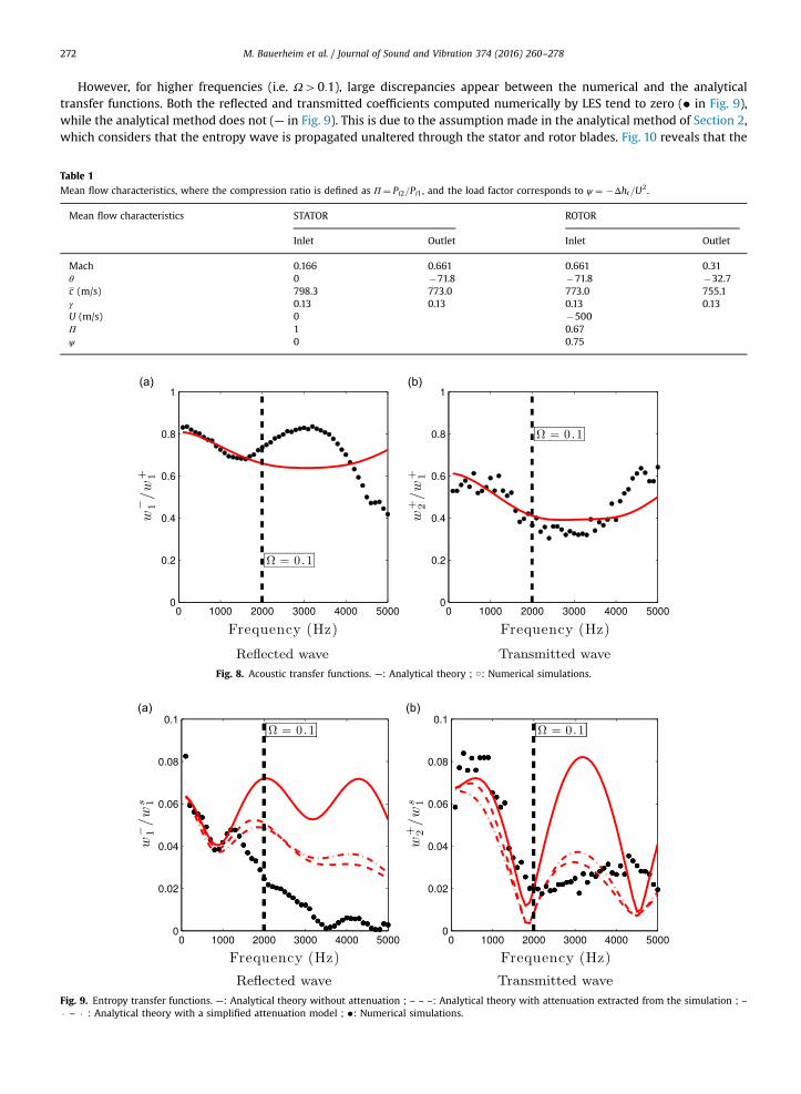
The mean flow characteristics are given in Table 1. Using these mean flow variables, the analytical model described inSection 2 is used to compute the acoustic and entropy transfer functions of the turbine stage. The acoustic reflection andtransmission coefficients are plotted in Fig. 8, comparing the analytical method with the numerical simulations of thestator–rotor stage. As previously mentioned, even if the analytical theory is frequency-dependent, the method is still basedon the compact assumption and therefore is strictly valid only for low frequencies. Yet, noticeably, the method performswell for frequencies ranging from 0 to 2000 Hz, and even up to 4000 Hz in the case of the transmitted wave. The value of thereduced frequency Ω¼ flx=c obtained using the stator axial length lx is also plotted. The analytical method is seen to predictthe transmitted and reflected acoustic waves within reasonable accuracy for at least Ωo0:1.

Similar results are obtained for the entropy transfer functions dedicated to indirect combustion noise (Fig. 9). Theanalytical method and the numerical simulations are again seen to agree for the low frequency range (i.e. Ωo0:1), wherethe compact assumption holds.

M. Bauerheim et al. / Journal of Sound and Vibration 374 (2016) 260–278272

However, for higher frequencies (i.e. Ω40:1), large discrepancies appear between the numerical and the analyticaltransfer functions. Both the reflected and transmitted coefficients computed numerically by LES tend to zero (� in Fig. 9),while the analytical method does not (— in Fig. 9). This is due to the assumption made in the analytical method of Section 2,which considers that the entropy wave is propagated unaltered through the stator and rotor blades. Fig. 10 reveals that the

Fig. 8. Acoustic transfer functions. —: Analytical theory ; ○: Numerical simulations.

Fig. 9. Entropy transfer functions. —: Analytical theory without attenuation ; – – –: Analytical theory with attenuation extracted from the simulation ; –� – � : Analytical theory with a simplified attenuation model ; �: Numerical simulations.

Table 1

Mean flow characteristics, where the compression ratio is defined as Π ¼ Pi2=Pi1, and the load factor corresponds to ψ ¼ �Δht=U2.

Mean flow characteristics STATOR ROTOR

Inlet Outlet Inlet Outlet

Mach 0.166 0.661 0.661 0.31θ 0 �71.8 �71.8 �32.7c (m/s) 798.3 773.0 773.0 755.1γ 0.13 0.13 0.13 0.13U (m/s) 0 �500Π 1 0.67ψ 0 0.75

M. Bauerheim et al. / Journal of Sound and Vibration 374 (2016) 260–278 273

entropy spot is not conserved through the stages. This was already observed by Leyko et al. [23] for the case of a single statorblade. The initial planar entropy waves are distorted by the 2D mean flow. Indeed, the potential flow induced by the thickblade under an incident flow, combined with the no-slip conditions on the stator and rotor blades, imposes an azimuthaldependency (y) of the mean flow, which has been neglected in the analytical model. This 2D flow prescribes a propagatingvelocity to the entropy wave which is dependent on the azimuthal direction, deforming the initial planar front at the length-scale of the pitch length, ly. It is worth noting that the total entropy fluctuation is not dissipated, but re-distributed inhigher-order propagating modes. Actual entropy dissipation caused by turbulent mixing may also exist in the simulation,but is not accounted for in the theoretical analysis performed here, since it requires a realistic 3D simulation.

Leyko et al. [23] used the mean flow through the stator blade to predict the decrease of the plane entropy waveamplitude at the outlet of a stator blade. The streamlines for the stator and the rotor cases are shown in Figs. 11a and b.Using this mean flow quantity (which could be computed by RANS simulations to reduce costs), a delay td(y) in arrival of thestreamlines at the outlet can be calculated (— in Fig. 12). From this time-delay, Leyko et al. [23] computed the attenuation ofthe planar mode propagating through the stator,

D0 fð Þ ¼ 1ly

Z ly

0exp 2πiftd yð Þ� �

dy����:

����� (58)

This attenuation function is displayed in Fig. 13 (—) for the stator stage. The total entropy dissipation of the first mode canbe obtained as a convolution product of both rotor and stator transfer functions, which in the frequency domain results intheir standard multiplication. The result is shown in Fig. 10 (– – –), as a function of the frequency. It exemplifies that at zero

Fig. 10. Entropy transmission through the stator–rotor. —: Analytical theory without attenuation; – – –: Analytical theory with attenuation extracted fromthe simulation ; – � – � : Analytical theory with a simplified attenuation model ; �: Numerical simulations.

Fig. 11. Streamlines through the turbine blades obtained using the mean flow.

Fig. 12. Time-delay td(y) obtained using the LES mean flow (—), and a simplified analytical profile (– – –). Note that y=ly ¼ 0 (respectively y=ly ¼ 1)corresponds to the suction side (respectively pressure side) for the stator blade, and to the pressure side (respectively suction side) for the rotor blade.

Fig. 13. A parametric study on the asymmetry (η¼ 0:1, 0.2, 0.3, and 0.4, left) and flatness (ng¼1, 2, 3, and 4, right) of the velocity profile on the attenuationof the entropy transmission through this single row.

M. Bauerheim et al. / Journal of Sound and Vibration 374 (2016) 260–278274

frequency, entropy waves propagate unaltered (no attenuation), but are attenuated for higher frequencies when travelingthrough the turbine stage: this attenuation model improves the analytical method accuracy. Both transfer functions areinjected into the analytical model of Section 2 to provide the entropy transfer functions when considering the entropydissipation (– – – in Fig. 9). It yields a better agreement with numerical results, especially at high frequencies (Ω40:1)where the entropy transmission tends to zero as the frequency increases due to the higher dissipation.

Even though this methodology accounting for entropy attenuation provides overall good results, it requires theknowledge of the delay in arrival time td(y), and therefore of the mean flow around each blade. In this study the attenuationfunction has been obtained using the LES mean field. A drastic cost reduction can be achieved by using RANS simulations,but it would be interesting to have a simple model in which td(y) (and therefore D0ðf Þ) could be computed without anynumerical simulations. In particular, the question on which parameter controlling the velocity profile affects actually theentropy deformation is still an open topic: typically, the flatness, or the asymmetry of the velocity profile are such potentialparameters, for which a generic analytical velocity profile can be used for parametric studies. As an example of such aninvestigation, the axial mean velocity wx is modeled here along the transverse direction y=ly using a generic asymmetricpower-law, such as

wxyly

� �¼ y

ly

�η=ng

1� yly

�ð1�ηÞ=ng

(59)

where η is the asymmetry parameter, controlling the location of the maximum velocity in the profile (½y=ly�max ¼ η), and ng isthe global power of the law. In the present stator–rotor configuration, nR

g ¼ 1 and ηR ¼ 0:8 for the rotor, and nSg ¼ 2 and

ηS ¼ 0:3 for the stator. These analytical models are compared with the delay td extracted from the simulation in Fig. 12.

M. Bauerheim et al. / Journal of Sound and Vibration 374 (2016) 260–278 275

Compared with numerical profiles, such theoretical models can be used for parametric studies, for example to analyze theeffects of flatness (ng) or asymmetry (η) on the wave damping function D0ðf Þ.

This model, proposed in Eq. (59), characterizes the mean axial velocity profile at which the entropy spot will propagate

through the turbine blade of length lx. The average mean flow w0x ¼ 1

ly

R ly0 wx y=ly

� �dy being known form the operating point,

the normalized time delay in arrival time tdf 0 is

td y=ly� �¼ lx

w0x

ηη=ng ð1�ηÞð1�ηÞ=ng

wxðy=lyÞ(60)

The time-delay td, obtained analytically using Eqs. (59)–(60), is compared with the time-delay extracted from the LESsimulation (— in Fig. 12), showing that simple generic profiles with two parameters (flatness and asymmetry) are sufficientto reproduce realistic mean profiles in a turbine stage. The theoretical attenuation function D0ðf Þ is then computed (Eq. (58))and injected in the model of Section 2. Predictions of this model for indirect noise (Fig. 9) and entropy transmission (Fig. 10)are compared with cases using (1) no attenuation (—) or (2) a numerical attenuation (– – –). It exemplifies that genericanalytical profiles can lead to overall good attenuation predictions, and therefore indirect noise estimations at thedesign stage.

When varying the asymmetry (η) and flatness ðngÞ of the modeled velocity profile, a parametric study of the attenuationfunction of entropy propagation can be performed, here restrained only to the stator vane for the sake of simplicity. First, theasymmetry is reduced by varying η from 0.1 (corresponding to a very asymmetric case, since η is the location of themaximum velocity in the profile) to 0.4 (almost symmetric case) . As expected, Fig. 13 (left) reveals that reducing theasymmetry of the mean velocity profile (η increases) also reduces the entropy attenuation. Similarly, when increasing theflatness of the velocity profile (ng increases), the attenuation is also reduced (Fig. 13, right). This simple analysis unveilsparameters controlling the attenuation function: when the asymmetry η, or the flatness ng , increased, they both yield moreuniform velocity profiles, and consequently lower attenuation functions. A further analysis is performed in Appendix B toshow explicitly the link between the mean axial flow profile and the attenuation behavior with frequency: at low frequency,only the mean velocity deficit is of significant importance, while at higher frequencies, an accurate velocity profile in theboundary layers is required.

This analysis demonstrates that the acoustic and entropy wave propagation and attenuation through a turbine stage canbe obtained analytically. It can be generalized for an arbitrary number of stages, as shown in Eq. (49), and therefore be usedas a predesign tool for core-engine noise.

5. Conclusions

Because of the modern design of combustion chambers to reduce pollution emissions and the new engine architectureswith more compact and highly loaded turbines, combustion noise arouses a novel interest. To complete analytical methodsused for acoustic (direct noise) and vorticity wave propagation through a stator vane developed in the seventies, the presentstudy revisits the compact theory proposed by Cumpsty and Marble into a general matrix form, formulation which alsotakes into account entropy waves to predict indirect noise. A generalization to rotating rows based on the conservation ofthe rothalpy is proposed to yield a complete propagation model through an entire turbine stage. Consequently, this paperfocuses on an analytical model taking into account the propagation of acoustic and vorticity as well as entropy wavesthrough a complete representative turbine stage, containing one stator followed by one rotor.

Such a methodology, termed CHORUS, allows the prediction of energy conversion from entropy to acoustics in a com-plete stage, leading to indirect noise in a full turbine. In particular, transfer functions characterizing transmission andreflection of waves are obtained analytically, and then compared with numerical predictions from forced compressibleLarge-Eddy Simulations of a 2D stator–rotor configuration. Numerically, the rotation is addressed by a fluid–fluid couplingstrategy with an overset-grid method, termed MISCOG, which has been developed recently and shown to yield goodtransmission properties in a rotor alone [43]. As expected from the compact assumption in the analytical model, its resultsagree with the simulation ones at low frequencies only, up to a reduced frequency based on the stator chord length ΩC0:1.This is mostly the case for the acoustic reflection coefficient and the entropy transmission coefficient. For the acoustictransmission coefficient the frequency range is slightly larger whereas it is narrower for the entropy reflection coefficient.This is consistent with what was found previously by Leyko et al. [23] for a stator vane only.

To improve the indirect noise predictions, the attenuation of entropy spots caused by their deformation through thestator vane or the rotor blade is also considered. As proposed by Leyko et al. [23] it is modeled by time-delays of arrival atthe blade outlet, which can be either extracted from the simulations or modeled through an analytical mean axial velocityprofile. Even though the latter does not reproduce all the features of the actual distortion in a turbine blade passage, italready includes several parameters that describe the asymmetry (or skewness) and the flatness of this velocity profile. Boththe analytical and numerical attenuation improve the indirect noise prediction drastically. Moreover, it is shown in a simpleparametric study that the flatness of the mean flow speed and its asymmetry are key parameters controlling the entropywave attenuation, and therefore indirect noise. A further analysis is developed revealing the link between the mean axialvelocity profile and the attenuation behavior with frequency. Results show that at low frequencies, only the mean velocity

M. Bauerheim et al. / Journal of Sound and Vibration 374 (2016) 260–278276

deficit is of importance, while at higher frequencies the attenuation is controlled by delay times on arrival in the boundarylayers. The complete analytical model already provides a reasonable agreement with 2D simulations, which allows theprediction and minimization of both direct and indirect noise at the design-stage without computation.

Appendix A. Fluctuation of the direction of the relative velocity

For the rotor, the fluctuation of the direction of the relative velocity ðθ0Þr has to be related to the fixed reference-framevariables θ0 and w0=w (Eq. (44)). The sine law in Fig. 2 gives

Usin ðθ�θrÞ ¼

wcos ðθrÞ; (A.1)

which can be differentiated to obtain an equation for the fluctuation of the direction of the relative velocity θ0ð Þr

θ0 � θ0ð Þr� �cos θ�θ

r�

¼ U

w2 � θ0ð Þr sin ðθrÞw�w0 cos ðθrÞh i

: (A.2)

Al-Kashi cosine laws yield

cos θ�θr

� ¼

wr� �2þ w2�U2�

2wwr ¼wrþU sin θ

r�

w; (A.3)

which allows the simplification of Eq. (A.2) into

θ0ð Þr ¼ θ0 1þ Uwr sin θr

� � �þ w0

w

� �Uwr cos θr

� : (A.4)

Appendix B. Effect of the mean axial flow on the attenuation function

The attenuation function D0ðf Þ, to account for the entropy spot distortion through the blades, is based on the delay-timeon arrival τdðy=lyÞ extracted in the LES or modeled analytically. This function defined in Eq. (58) is recalled here:

D0 fð Þ ¼ 1ly

Z ly

0e2πif τd yð Þ dy

����:����� (B.1)

An open question is to understand the effect of the mean axial velocity profile wxðy=lyÞ, or the time on arrival profileτdðy=lyÞ, on this attenuation function. The results of the parametric study (Fig. 13) have shown the crucial role of asymmetryη and flatness ng on the global attenuation level, but explicit relations between D0ðf Þ and τdðy=lyÞ are still required tounderstand the attenuation behavior with frequency. For instance, knowing which parameters control the attenuation atlow and high frequencies, and whether these parameters are identical in both frequency ranges, is a key information tounderstand mechanisms leading to attenuation and to improve modeling. Writing the exponential function as a powerseries and using Fubini's theorem to switch the integral–summation order, the attenuation function can be recast as

D0 fð Þ ¼X1

k ¼ 0

ði2πf Þkk!

Z 1

0τdðy=lyÞk d y=ly

� � ¼X1

k ¼ 0

f k

k!∂kD0

∂f kf ¼ 0ð Þ

�����:�����

���������� (B.2)

Eq. (B.2) reveals explicitly the link between the time on arrival profile τd and the behavior of the attenuation function

through its derivatives ∂kD0

∂f k. Note that Eq. (B.2) corresponds to a Taylor expansion of D0ðf Þ, and is therefore equivalent to Eq.

(58). It can be simplified using only the first N terms of the summation: the truncated relation is then only an approximationof Eq. (58) on the low frequency range ½0; f N�, where f N can be made as large as desired by adding a sufficiently large numberof terms N (Fig. 14a).

Nevertheless, compared with Eqs. (58), (B.2) provides some insight on the variation of the attenuation function withfrequency. First, the zero-frequency limit is straightforward, since at f ¼ 0 only the term k¼ 0 exists, leading tolimf-0D0ðf Þ ¼ 1, which confirms that the entropy spot propagates through the turbine stage without distortion at a nullfrequency (compact assumption). Second, close to the zero-frequency limit, the behavior of D0ðf Þ is governed by the term

k¼ 1, which can be written as 2πif ⟨τd⟩, where ⟨τd⟩¼R 10 τd y=ly

� �d y=ly� �

corresponds to the mean delay-time on arrival. Theslope of the attenuation function at the zero-frequency limit is therefore shown to be only governed by this mean delaytime. Moreover, this truncated expression suggests that the behavior of D0ðf Þ at higher frequencies depends only on themean quantities ⟨τkd⟩. This result is exemplified in Fig. 14b where the first 26 terms of Eq. (B.2) are displayed for threedifferent frequencies: at null frequency ðf ¼ 0 HzÞ, at moderate frequencies ðf ¼ 2000 HzÞ, and finally at high frequenciesðf ¼ 4000 HzÞ. It indicates that at null frequency ðf ¼ 0Þ, only the mean delay-time on arrival is of significant importance(term k¼ 1, since for k¼ 0 the coefficient is unity). At moderate frequencies ðf ¼ 2000 HzÞ, ⟨τd⟩ is still dominant, but higher

Fig. 14. (a) Attenuation function of the stator extracted from the LES using Eq. (58) displayed by the solid line, and the truncated relation using 26 terms ofEq. (B.2), displayed by a dashed line with circles. (b) Coefficients ð2πf Þk⟨τkd⟩=k! estimated at three different frequencies f :0 Hz;2000 Hz, and 4000 Hz for thecoefficients k¼0–25.

M. Bauerheim et al. / Journal of Sound and Vibration 374 (2016) 260–278 277

harmonics also appear. Since the mean delay-time ⟨τd⟩ is dominant at low frequencies, it shows that the transverse profile isnot necessary: only the mean velocity deficit is needed. However, at high frequencies ðf ¼ 4000 HzÞ, the mean profile ðk¼ 1Þdoes not affect the attenuation anymore. The larger coefficient is found around k¼ 9, meaning that ⟨τ9d⟩ is of significant

importance: since τd is null near the centerline of the blade, but maximal at walls, it suggests that ⟨τ9d⟩, and therefore theattenuation function at high frequencies, is governed by delay-times in the boundary layers: wall-resolved simulations aremandatory to capture correctly the entropy wave deformation at high frequencies. Typically in the stator case, the whole

normalized profile fτd=maxðτdÞg9 is below 0.001 except in the layer y=lyA ½0:975;1�.

References

[1] H.M. Atassi, A.A. Ali, O.V. Atassi, I.V. Vinogradov, Scattering of incident disturbances by an annular cascade in a swirling flow, Journal of Fluid Mechanics499 (2004) 111–138.

[2] AVBP code: ⟨http://cerfacs.fr/logiciels-de-simulation-pour-la-mecanique-des-fluides/⟩ and ⟨http://cerfacs.fr/publication/⟩.[3] F. Bake, C. Richter, B. Muhlbauer, N. Kings, I. Rohle, F. Thiele, B. Noll, The entropy wave generator (ewg): a reference case on entropy noise, Journal of

Sound and Vibration (2009) 574–598.[4] D. Blacodon, S. Lewy, Source localization of turboshaft engine broadband noise using a three-sensor coherence method, Journal of Sound and Vibration

338 (17) (2015) 250–262.[5] C. Bosman, C.O. Jadayel, A quantified study of rothalpy conservation in turbomachines, International Journal of Heat and Fluid Flow 17 (4) (1996)

410–417.[6] S. Candel, Acoustic transmission and reflection by a shear discontinuity separating hot and cold regions, Journal of Sound and Vibration 24 (1972) 87–91.[7] B.T. Chu, L.S.G. Kovasznay, Non-linear interactions in a viscous heat-conducting compressible gas, Journal of Fluid Mechanics 3 (1958) 494–514.[8] O. Colin, M. Rudgyard, Development of high-order Taylor–Galerkin schemes for unsteady calculations, Journal of Computational Physics 162 (2) (2000)

338–371.

M. Bauerheim et al. / Journal of Sound and Vibration 374 (2016) 260–278278

[9] N.A. Cumpsty, F.E. Marble, The interaction of entropy fluctuations with turbine blade rows; a mechanism of turbojet engine noise, Proceedings of theRoyal Society of London A 357 (1977) 323–344.

[10] J. Donea, L. Quartapelle, V. Selmin, An analysis of time discretization in the finite element solution of hyperbolic problems, Journal of ComputationalPhysics 70 (1987) 463–499.

[11] I. Duran, Prediction of Combustion Noise in Modern Aero Engines Combining LES Simulations and Analytical Methods, PhD Thesis, INP Toulouse, 2013.[12] I. Duran, S. Moreau, Numerical simulation of acoustic and entropy waves propagating through turbine blades, 19th AIAA/CEAS Aeroacoustics Conference,

AIAA 2013-2102 paper, Colorado Springs, CO, 2013.[13] I. Duran, S. Moreau, Solution of the quasi one-dimensional linearized Euler equations using flow invariants and the Magnus expansion, Journal of Fluid

Mechanics 723 (2013) 190–231.[14] I. Duran, S. Moreau, T. Poinsot, Analytical and numerical study of combustion noise through a subsonic nozzle, AIAA Journal 51 (1) (2013) 42–52.[15] A. Giauque, M. Huet, F. Clero, Analytical analysis of indirect combustion noise in subcritical nozzles, Journal of Engineering for Gas Turbines and Power

134 (11) (2012) 111202.[16] A. Giauque, M. Huet, F. Clero, Analytical analysis of indirect combustion noise in subcritical nozzles, Proceedings of ASME TURBO EXPO, 2012, pp. 1–16.[17] C.S. Goh, A.S. Morgans, Phase prediction of the response of choked nozzles to entropy and acoustic disturbances, Journal of Sound and Vibration 330

(21) (2011) 5184–5198.[18] M.S. Howe, Indirect combustion noise, Journal of Fluid Mechanics 659 (2010) 267–288.[19] M. Ihme, H. Pitsch, On the generation of direct combustion noise in turbulent non-premixed flames, International Journal of Aeroacoustics 11 (1) (2012)

25–78.[20] S. Kaji, T. Okazaki, Propagation of sound waves through a blade row: I. Analysis based on the semi-actuator disk theory, Journal of Sound and Vibration 11

(3) (1970) 339–353.[21] S. Kaji, T. Okazaki, Propagation of sound waves through a blade row: II. Analysis based on acceleration potential method, Journal of Sound and Vibration

11 (3) (1970) 355–375.[22] N. Lamarque, T. Poinsot, Boundary conditions for acoustic eigenmodes computation in gas turbine combustion chambers, AIAA Journal 46 (9) (2008)

2282–2292.[23] M. Leyko, I. Duran, S. Moreau, F. Nicoud, T. Poinsot, Simulation and modelling of the waves transmission and generation in a stator blade row in a

combustion-noise framework, Journal of Sound and Vibration 333 (23) (2014) 6090–6106.[24] M. Leyko, S. Moreau, F. Nicoud, T. Poinsot, Waves transmission and generation in turbine stages in a combustion-noise framework, 16th AIAA/CEAS

AeroAcoustics Conference, AIAA 2010-4032 paper, Stockholm, Sweden, 2010.[25] M. Leyko, F. Nicoud, S. Moreau, T. Poinsot, Numerical and analytical investigation of the indirect noise in a nozzle, Proceedings of the Summer Program,

Center for Turbulence Research, NASA AMES, Stanford University, USA, 2008, pp. 343–354.[26] M. Leyko, F. Nicoud, T. Poinsot, Comparison of direct and indirect combustion noise mechanisms in a model combustor, AIAA Journal 47 (11) (2009)

2709–2716.[27] M.J. Lighthill, On sound generated aerodynamically. i. General theory, Proceedings of the Royal Society of London A, Mathematical and Physical Sciences

211 (1107) (1952) 564–587.[28] T. Livebardon, Modeling of Combustion Noise in Helicopter Engines, PhD Thesis, INP Toulouse, 2015.[29] T. Livebardon, S. Moreau, L. Gicquel, T. Poinsot, E. Bouty, Combining les of combustion chamber and an actuator disk theory to predict combustion

noise in a helicopter engine, Combustion and Flame 165 (2016) 272–287.[30] F.A. Lyman, On the conservation of rothalpy in turbomachines, Journal of Turbomachinery 115 (3) (1993) 520–525.[31] F.E. Marble, S. Candel, Acoustic disturbances from gas nonuniformities convected through a nozzle, Journal of Sound and Vibration 55 (1977) 225–243.[32] R.S. Muir, The application of a semi-actuator disk model to sound transmission calculations in turbomachinery, part i: the single blade row, Journal of

Sound and Vibration 54 (3) (1977) 393–408.[33] R.S. Muir, The application of a semi-actuator disk model to sound transmission calculations in turbomachinery, part ii: multiple blade rows, Journal of

Sound and Vibration 55 (3) (1977) 335–349.[34] M. Muthukrishnan, W.C. Strahle, D.H. Neale, Separation of hydrodynamic, entropy, and combustion noise in a gas turbine combustor, AIAA Journal 16

(4) (1978) 320–327.[35] G.F. Pickett, Core engine noise due to temperature fluctuations convecting through turbine blade rows, 2nd AIAA Aeroacoustics Conference, AIAA 1975-

528 paper, Hampton, VA, 1975.[36] T. Poinsot, S. Lele, Boundary conditions for direct simulations of compressible viscous flows, Journal of Computational Physics 101 (1) (1992) 104–129.[37] T. Schønfeld, M. Rudgyard, Steady and unsteady flows simulations using the hybrid flow solver avbp, AIAA Journal 37 (11) (1999) 1378–1385.[38] L. Selle, F. Nicoud, T. Poinsot, The actual impedance of non-reflecting boundary conditions: implications for the computation of resonators, AIAA Journal

42 (5) (2004) 958–964.[39] S.R. Stow, A.P. Dowling, T.P. Hynes, Reflection of circumferential modes in a choked nozzle, Journal of Fluid Mechanics 467 (2002) 215–239.[40] W.C. Strahle, On combustion generated noise, Journal of Fluid Mechanics 49 (1971) 399–414.[41] W.C. Strahle, Some results in combustion generated noise, Journal of Sound and Vibration 23 (1) (1972) 113–125.[42] C.K.W. Tam, S.A. Parrish, J. Xu, B. Schuster, Indirect combustion noise of auxiliary power units, Journal of Sound and Vibration 332 (17) (2013)

4004–4020.[43] G. Wang, F. Duchaine, D. Papadogianis, I. Duran, S. Moreau, L.Y.M. Gicquel, An overset grid method for large-eddy simulation of turbomachinery stages,

Journal of Computational Physics 274 (2014) 333–355.[44] C.S. Yoo, Y. Wang, A. Trouvé, H.G. Im, Characteristic boundary conditions for direct simulations of turbulent counterflow flames, Combustion Theory and

Modelling 9 (2005) 617–646.