Journal of the Operations Research © 2001 The Operations ...archive/pdf/e_mag/Vol.44_01_019.pdf · Journal of the Operations Research Society of Japan Vol. 44, No. 1, March 2001

Journal of the Operations Research Society of Japan

Vol. 44, No. 1, March 2001.

THE VARIABLE LEAD TIME STOCHASTIC INVENTORY MODEL WITH A FUZZY BACKORDER RATE

Liang-Yuh Ouyang Hung-Chi Chang Tamkang University National Taichunq Institute of Technology

(Received July 12, 1999; Final September 4, 2000)

Abstract Cost and operation of inventory depends a great deal on what happens to demand when the system is out of stock. In real inventory systems, it is more reasonable to assume that part of the excess demand is backordered and the rest is lost. However, the amount of backorders (or lost sales) often incurs disturbance due to various uncertainties. To incorporate this reality, this article attempts to apply the fuzzy set concepts to deal with the uncertain backorders and lost sales. The purpose of this paper is to modify Moon and Choi's continuous review inventory model with variable lead time and partial backorders by fuzzifying the backorder rate (or equivalently, fuzzifying the lost sales rate). We first consider the case where the lost sales rate is treated as the triangular fuzzy number. Then, through the statistical method for establishing the interval estimation of the lost sales rate, we construct a new fuzzy number, namely statistic-fuzzy number. For each fuzzy case, we investigate a computing schema for the modified continuous review inventory model and develop an algorithm to find the optimal inventory strategy.

1. Introduction Traditionally, the economic order quantity (EOQ) model dealing with continuous review inventory problems assumed that demand during the stockout period is either completely backordered or completely lost; the lead time is viewed as a prescribed constant or a random variable, which there is not subject to control [13,18]. However, these are not quite practical. In real markets, we can often observe that, when the inventory system is out of stock, some of the customers are willing to wait for their demand, while others may fill their demand from another source. And hence, for inventory models in which shortages are allowed, it is more reasonable to assume that some of the excess demand is backordered and the rest is lost. In literature, several authors (e.g., Montgomery e t al. [Ill, Kim and Park [8] , Ouyang et al. [14], Moon and Choi [12] and Hariga and Ben-Daya [6]) have presented the inventory models with partial backorders, specifically, Montgomery e t al. [ll] is among the first who formulated and solved the continuous review, stochastic demand inventory problem.

On the other hand, as pointed out in Tersine [19], lead time usually consists of the following components : order preparation, order transit, supplier lead time, delivery time and setup time. In some cases, these components can be accomplished earlier than the regular time if one is willing to pay extra costs; in other words, lead time is controllable. For an example, one may adopt the special delivery (by air) instead of ordinary delivery (by water) to shorten the delivery time. Obviously, the air freight rate is higher than the water freight rate, and hence more money can be spent to shorten lead time. Also, through the Japanese successful experiences of using Just-In-Time (JIT) production, the advantages and benefits associated with efforts to reduce lead time have been evidenced. Lead time reduction has received a lot of interest in recent years. Liao and Shyu [lo] first presented a probabilistic inventory model in which the order quantity is predetermined and lead time

© 2001 The Operations Research Society of Japan

20 L.- Y Ouyang & H.-C. Chang

is a unique variable. Ben-Daya and Raouf [l] extended Liao and Shyu's [lo] model by considering both lead time and order quantity as decision variables. Ouyang et al. [14] generalized Ben-Daya and Raouf's [I] model by allowing shortages with partial backorders. Recently, Moon and Choi [12] and Hariga and Ben-Daya [6] further extended Ouyang et al.'s [14] model by considering the reorder point as one of the decision variables.

We note that the underlying assumption in above partial backorder models, no matter with lead time reduction [6, 12, 141 or not [8, 111, is that the fraction of excess demand backordered (or lost) is a fixed constant. However, in the real situation, when stockout occurs many potential factors such as properties of products and/or image of selling shop may affect customers9 wills of backorders. In other words, the amount of lost demand caused by stockout probably has a little disturbance due to various uncertainties. Therefore, if we express the fuzzy backorder (or lost sales) rate as the neighborhood of the fixed backorder (or lost sales) rate, then it will more match with the real situation.

In fact, the application of fuzzy set concepts on EOQ inventory models have been proposed by many authors (e.g., Park [15], Chen et al. [3], Yao and Lee [20], Roy and Maiti [16], Chang et al. [2], Lee and Yao [9]). Specifically, Yao and Lee [20] used the extension principle to solve the inventory model with shortages by fuzzifying the order quantity, in which the shortage quantity is a real variable. Later, Chang et al. [2] fuzzified the shortage quantity in the backorder model, where the order quantity is a real variable. Inventory model without backorder is discussed by Lee and Yao [9], who fuzzify the order quantity to a fuzzy number, and solve the economic order quantity with the extension principle. However, these studies [2, 3, 9, 15, 16, 201 are almost concentrated on the simple EOQ forms so that there has few applications in the real inventory systems. The purpose of this paper is to present a more extensive EOQ model to modify Moon and Choi's [12] model by fuzzifying the lost sales rate and to solve this new inventory model in the fuzzy sense.

In this paper, we study the continuous review (Q, r ) inventory models with partial backorders, where the lead time is viewed as a controllable variable and two fuzziness of lost sales rate are introduced. Firstly, we express the lost sales rate as one of the widely used fuzzy numbers, namely the triangular fuzzy number. Then, by employing the statistical method we construct a confidence interval for the lost sales rate, and through it to establish the corresponding fuzzy number called the statistic-fuzzy number. It is noted that the statistical technology has often been utilized to solve the problem with uncertainty in many research areas including Operations Research. Furthermore, this paper investigates a computing schema for each fuzzy case and develops an algorithm procedure to find the optimal inventory strategy. Two examples are given to illustrate the results derived and concluding remarks are made.

2. Membership Function of the Fuzzy Total Cost First of all, the following notations and assumptions are employed thoughout this paper so as to develop the proposed models.

Notations : Q = order quantity A = ordering cost r = reorder point L = length of lead time D = annual demand rate h = annual inventory holding cost per unit

Copyright © by ORSJ. Unauthorized reproduction of this article is prohibited.

Inventory Model with a Fuzzy Backorder Rate

7~ = fixed penalty cost per unit short

TO = marginal profit per unit

Q = fraction of the shortage that will be backordered, 0 < Q < 1 X = the lead time demand which has a probability density function (p.d.f.)

f (-) with finite mean D - L and standard deviation a - a, where a denotes the standard deviation of the demand per unit time

B ( r ) = the expected demand shortage at the end of the cycle

Assumptions

The reorder point r = expected demand during lead time + safety stock (SS), and SS = k - (standard deviation of lead time demand), i.e., r = DL + k o a , where k is the safety factor.

Inventory is continuously reviewed and replenishments are made whenever the inventory level falls to the reorder point r . The lead time L has n mutually independent components. The ith component has a

minimum duration a; and normal duration bi, and a crashing cost per unit time ci. Furthermore, for convenience, we rearrange c; such that ci < cz < - - - < en. Then, it is clear that the reduction of lead time should first occur on component 1 (because it has the minimum unit crashing cost), and then component 2, etc.

n

If we let Lo = x by and L; be the length of lead time with components 1 , 2 , - - - , i crashed y = 1

n i

to their minimum duration, then L; can be expressed as Li = x by - E(bj - a,), 2" = 1, j=1 y = 1

2, - - . , n; and the lead time crashing cost R(L) per cycle for a given L â [Li, Li-l]7 is given by

i- 1

R(L) = ci(Li-1 - L) + cj(bj - a,) and R(Lo) = 0. y= 1

For the model in which the order quantity, Q, reorder point, r , and lead time, L are treated as decision variables, we will closely follow Moon and Choi [12]. Specifically, by assumptions 1-4, the total expected annual cost, which is composed of ordering cost, inventory holding cost, stockout cost and lead time crashing cost, is expressed by

Now we attempt to modify Moon and Choi7s [12] model by fuzzifying the backorder rate (or equivalently, fuzzif~ing the lost sales rate). For convenience, we first let 5 2 1 - /3 denote the lost sales rate. Therefore, for any Q > 0, r > 0 and L > 0, we may rewrite the expected annual total cost function (1) as follows

Note that in above model, the lost sales rate 5 during the planning horizon is assumed to be a fixed constant. However, when the inventory planning is completed, due to various uncertainties the lost sales rate in practical problem may be not equal to 5 but just close to it. This scenario can be expressed in fuzzy language as " 6 = the real lost sales rate is


22 L. - Y. Ouyang & H. -C. Chang

around S ". Therefore, we would like to replace the lost sales rate S by the fuzzy number 8, and consider it as the triangular fuzzy number, 8 = (6 - Al, 6, S + As), where 0 < Al < 5 and 0 < A2 < 1 - 6, Al and A2 are determined by the decision-makers. Also, here we describe the membership function of S as follows:

^2

0, otherwise.

The pictorial sees Figure 1. Then the centroid (see, e.g. [4,~.336]) for /-^(a;) is given by

We regard this value as the estimate of lost sales rate in the fuzzy sense.

'r

- Figure 1: Triangular fuzzy number S

For any Q > 0, r > 0 and L > 0, we let C(Q,r,L)(x) = y (> 0). By extension principle 7 , 211, the membership function of the fuzzy cost CIQ,r,L) (8) is given by

From C ( Q , ~ , ~ ) ( X ) = y and equation (2), we get

Consequently, Q

Y Q - [ W D + ~ Q ( ~ + ~ - D L ) ] x =

(hQ + roD)B(r) 7 ( 7 )

where W = A + R(L) + 7rB(r). Therefore, from (3) and ( 7 ) , the membership function of CIQ,r,L}(S) can be written as



where

and

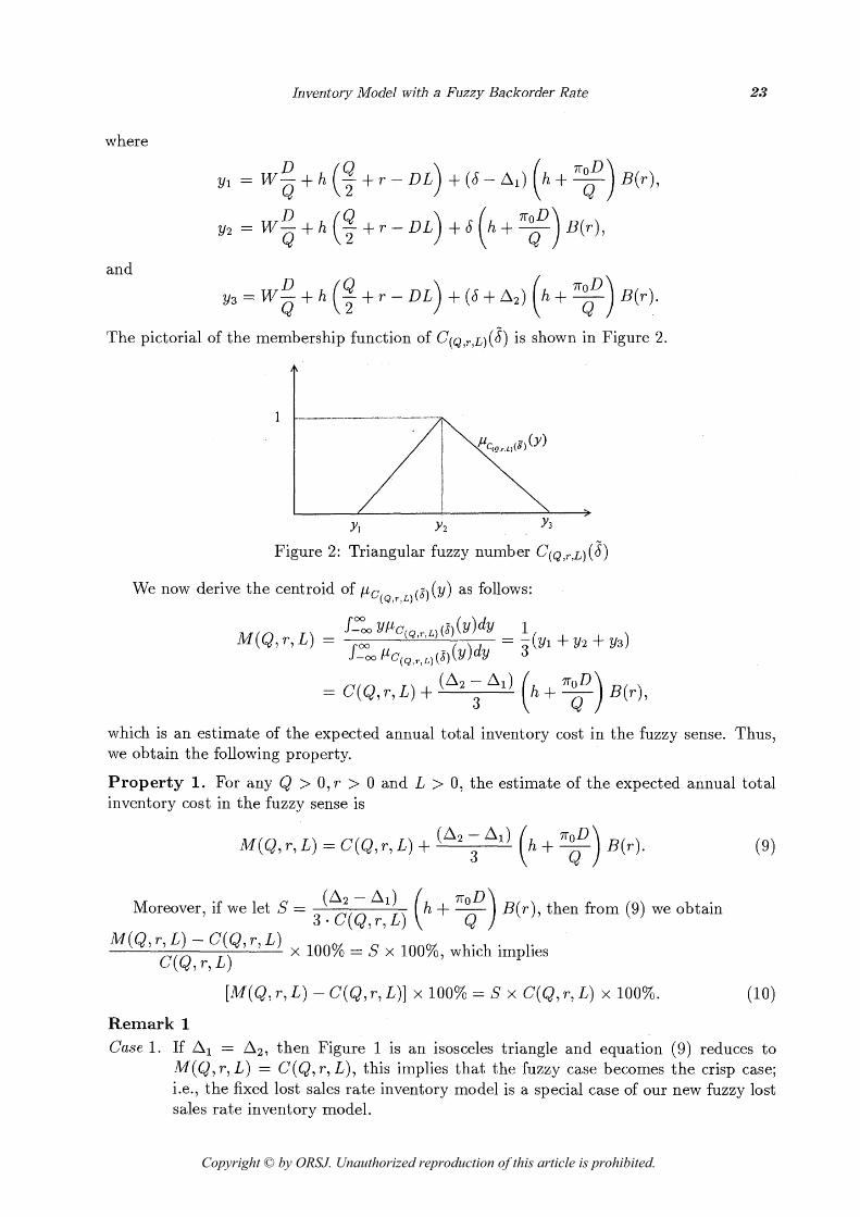
The pictorial of the membership function of C ~ ~ , ~ , ~ ) ( S ) is shown in Figure 2.

Y l Vi Y 3

Figure 2: Triangular fuzzy number c ( ~ , ~ , ~ ) (8)

We now derive the centroid of I J . ~ ( ~ , ~ , ~ ) ( ~ ) { ~ ) as follows:

which is an estimate of the expected annual total inventory cost in the fuzzy sense. Thus, we obtain the following property.

Property 1. For any Q > O,r > 0 and L > 0, the estimate of the expected annual total inventory cost in the fuzzy sense is

Moreover, if we let S = (A2 - Ai) (h + y) B(r), then from (9) we obtain

3 C(Q7r , L)

M(Q' r' L, - C(Q7 r7 L, x 100% = S x loo%, which implies C(Q, r, L)

[M(Q, r , L) - C(Q,r , L)] x 100% = S x C(Q, r, L) x 100%. (10)

Remark 1

Case 1. If Al = A2, then Figure 1 is an isosceles triangle and equation (9) reduces to M(Q, r, L) = C(Q, r, L), this implies that the fuzzy case becomes the crisp case; i.e., the fixed lost sales rate inventory model is a special case of our new fuzzy lost sales rate inventory model.



Case 2. If A l < Aa, then the triangle in Figure 1 is skewed to the right. In this case, M(Q, r , L) > C(Q, r, L) and the increment of M(Q, r, L) is S% of C(Q, r, L) (from

(10)). Case 3. If Ai > A2, then the triangle in Figure 1 is skewed to the left. In this case,

M(Q, r, L) < C ( Q , r , L) and the decrement of M ( Q , r , L) is 15'1% of C(Q, r, L) (from (10)).

3. Optimal Solution This section investigates the optimal inventory strategy in the fuzzy sense for a situation where the lead time demand, X, follows a normal distribution with p.d. f. f (-), mean DL and standard deviation a /L. We note that the reorder point r = DL + ko-^/L (assumption (i)) and the expected number of shortages at the end of the cycle B ( r ) = fm (x - r ) f (x)dx =

a /L{(i,(k) - k [ l - a(&)]} = vfi'S{k), where of.) and a ( - ) denote the standard normal p.d. f . and c.d. f . (cumulative distribution function), respectively, and Q(k) = (i,(k) - k[1 - @(k)].

Following the above result, we can allow the safety factor k as a decision variable instead of the reorder point r . Therefore, our problem of determining the optimal ( Q , r , L) by minimizing (9) can be reduced to minimizing

over Q , k and L. To solve this problem, we first note that M(Q, k, L) is concave in L E [Lh for fixed

(Q, k) because

Hence, for fixed (Q, k), the minimum expected annual total cost in fuzzy sense will occur at the end points of the interval [Li, L;-l]. On the other hand, it can be shown that M(Q, k, L) is convex in (Q, k) for fixed L 6 [L;, (see Appendix for the proof). Hence, for fixed L 6 [L;, LiF1], the minimum value of M (Q, k, L) will occur at the point (Q, k), say (Q*, k*), which satisfying 9 M ( Q , k, L) /9Q = 0 and 9M[Q, k, L)/9k = 0, simultaneously. Solving these two equations result in

and

^(k) = 1 - hQ (13)

T D + (hQ + TOD) ( 6 + From equations (12) and (13), though it is difficult to find the closed-form solution of

(Q*, k*), however, the optimal value of (Q*, k* ) can be obtained using the iterative procedure



(see, e.g. Hadley and Whitin [5]). Therefore, the following algorithm to find the optimal solutions for the order quantity, safety factor, and lead time can be developed.

Algorithm 1

Step 1. For given L;, i = 0,1,2, - - - , n, perform (i) to (iv).

(i) Start with kil = 0 and get Â¥S(kii = 0.39894 (which can be obtained by consulting the normal table ^>(kii) = 0.39894 and @(kil) = 0.5).

(ii) Substituting l'(kil) into (1 2) evaluates Qil . (iii) Utilizing Qil determines <E'(ki2) from (11), then finds I& by consulting the normal

table, and hence Â¥S(ki2) (iv) Repeat (ii) to (iii) until no change occurs in the values of Qi and ki.

Denote the solution by (Q:, k*).

Step 2. For each (QT, k:, L;) , ?' = 0,1,2, - . , n, calculate the corresponding fuzzy expected annual total inventory cost M(QT k * Li) by utilizing (1 1).

Step3. Find min M(Q:,k,",Li). I f M ( Q t , k r , L 8 ) = , min M(Q:,k,*,Li), then(Qi7 i=O,1,2,Â¥-, z = O , l , 2 , - ~ ~ , n

kg, Lr) is the optimal solution in the fuzzy sense. Once kc and Lr are obtained, the

optimal reorder point r-8 = D Lg + $0 L- follows. v Example 1. In order to illustrate the above solution procedure, let us consider an inventory system with the data used in Moon and Choi ([12], which is the same as in Ouyang et al. [14]): D = 600 units per year, A = $200 per order, h = $20 per unit per year, TT = $50 per unit short, TTQ = $150 per unit lost, 0 = 7 units per week, and the lead time has three components with data shown in Table 1.

Table 1: Lead time data Lead time Normal duration Minimum duration Unit crashing

component i bi (days) ai (days) cost ci($ /day) 1 2 0 6 0.4 2 20 6 1.2 3 16 9 5 .O

Here, we consider three cases: (Ai, A2) = (0.2,0.2), (Ai , Aa) = (0.1,0.4), and (Ai, A,) = (0.4,O.l). We solve each case for lost sales rate 8 = 0.5. The results of the solution procedure are summarized in Table 2.

From Table 2, when Al = A2 = 0.2 (in this situation, the fuzzy case becomes the crisp case), by comparing M(Q:, r;, LA, i = 0,1,2,3, we obtain the optimal solution (Qg, kr, Lg) = (121,72,4) and the minimum expected annual total cost in fuzzy sense M(Q;, kg, Lr) = $2941.68, which are the same as showed w in Moon and Choi [12]. Moreover, when A1 = 0.1 and A2 = 0.4, i.e., the fuzzy number 8 = (0.4,0.5,0.9), we have (Qs, r l , Lr) =

(121,73,4) and M(Qs7r8, L8) = $2954.09. Note that since C(Qs, r., Ls) = $2941.68 is the corresponding minimum expected annual total cost in the crisp case, and hence the absolute relative variation in the fuzzy sense for the minimum expected annual total cost is

Similarly, for the case Al = 0.4 and A2 = 0.1, i.e., the fuzzy number 8 = (0.1,0.5,0.6), we have (Qg, rg, Lr) = (121,71,4) and M(Qs,r,, Lj) = $2927.42, and the absolute relative


L. - Y. Ouyang & H. -C. Chang

Table 2: Solution procedure of Algorithm 1 (Li in weeks)

A1 A2 i Li R(L4 Q: rf (kf) M(Qr, r f , Li) 0.2 0.2 0 8 0.0 117 129 (1.8689) $ 3090.09

variation in the fuzzy sense for the minimum expected annual total cost is

4. Using the Sample Data to Fuzzify the Lost Sales Rate In general, the real lost sales rate 8 is unknown in advance. In order to estimate the value of 8, intuitively, one may collect the random sample data of lost sales rate from past time, then compute the mean of the sample measurement (say S) and use it as the estimate of 8. Such an issue belongs to the statistical problem. Moreover, though it can be shown that S is a good point estimator of 8, however, when the inventory planning is completed, the lost sales rate in practical problem may not equal to 6 but just close to it. This scenario can be described in fuzzy language as " S* = the real lost sales rate is around S ". Therefore, we need to combine the statistical and fuzzy technologies to deal with such an inventory problem. This section tackles this problem and the procedures are as follows.

Assume the actual lost sales rate 6 (which can be regarded as the population mean of lost sales rate) is unknown, and suppose we have collected m random sample data of lost

I m

sales rate during past time, say J1, 82, - - . , dm, then the sample mean is S = Ã x &, and rn =I

2 1 the sample variance is s = - x ( 8 ; - Q2. Furthermore, suppose the above sample m - 1 =1

data satisfy some certain statistical assumptions such as normality, then by the method for establishing the interval estimation of the parameter, we get the following (1 - a ) x 100% confidence interval for 6:

where cil, a 2 > 0, al + a2 = a, and tm-,(ai), i = 1,2, is the tabulated upper a, point of the t-distribution with m - 1 degrees of freedom; that is, if T be a random variable distributed as t-distribution with m - 1 degrees of freedom, then (ai) is the value that satisfies the following condition:

P I T > t m - l ( ~ ) ] = q i = 1 , 2 . (15)


Inventory Model with a Fuzzy Backorder Rate 27

Next, we take any point (denoted by $0) from the inside of above confidence interval (14). If So = 8, then the error of estimation \So - S\ = 0; in this case, the confidence level is viewed as 1. In contrast, the further the point & is from 5, the larger the error of estimation \So - $ 1 to be, and hence, the smaller the confidence level will be given. If So is one of the end points of the confidence interval, then the error of estimation [So - S\ is in the largest; in this case, the confidence level is viewed as 0. Thus, we can employ (14) to express the st at istical-fuzzy lost sales rate S* as the following triangular fuzzy number:

where a\ + a2 = a. Note that the decision-makers can determine a1 and a2 so as to satisfy

Remark 2. We note that since the membership grade of (16) has the same property as the above confidence level, so using confidence level as membership grade to construct the st at istic-fuzzy number (16) (corresponding to (14)) is feasible and validity.

The membership function of statistic-fuzzy lost sales rate S* is given by:

I 0, otherwise.

The pictorial sees Frgure 3. Then the centroid of ps* (x ) is

We regard this value as the estimate of lost sales rate in the fuzzy sense. Obviously, 6** > 0 -

and 6" belongs to the interval (14). For the special case a1 = a2 = al l , it gets 6" = 5-

Figure 3: Triangular fuzzy number S*



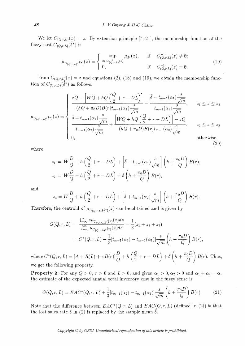
We let C(Q,~,L)(X) = z . By extension principle [7, 211, the membership function of the fuzzy cost c ( ~ , ~ , ~ ) (S*) is

From C(Q,r ,Lj (~) = z and equations (2), (18) and (19), we obtain the membership function of C(Q,r,L) (5*) as follows:

otherwise,

(20) where

and TI-0 D

[i;trn-1!.,2.^-] I'm ( h + T ) '('1.

Therefore, the centroid of (z) can be obtained and is given by

we get the following property.

Property 2. For any Q > 0, r > 0 and L > 0, and given a\ > 0 , ~ > 0 and a1 + a 2 = a , the estimate of the expected annual total inventory cost in the fuzzy sense is

Note that the difference between EAC*(Q, r , L) and EAC(Q, r , L) (defined in (2)) is that the lost sales rate S in (2) is replaced by the sample mean Z.


Inventory Mode1 with a Fuzzy Backorder Rate 29

Remark 3. If we let S* = [tm-l(a2) -tm-l(al)] s

- ( h + y) B(r) , then from (21) we 3EAC*(Q, r, L) v/m

obtain G(Q' r7 L, - EAc*(Q' x 100% = 5" x loo%, which implies EAC* (Q, r, L)

[G(Q, r , L) - EAC*(Q, r, L)] x 100% = S* x EAC*(Q, r, L) x 100%. (22)

Thus, we have the following results.

(i) If a1 = a 2 = a/2 , then tm_l(ai) = tm-i (a2), which implies G(Q, r, L) = EAC*(Q, r, L). That is, the total cost EAC*(Q, r, L) obtained by point estimate S is consistent with the total cost G(Q, r , L) obtained by fuzzy number S* defined in (16).

(ii) If 0 < a 2 < a1 < 1, then tm_l(al) < tm-1(a2), which implies G(Q, r, L) > EAC*(Q, r, L), and the increment of G(Q, r, L) is S*% of EAC* (Q, r, L).

(iii) If 0 < a1 < 0 2 < 1, then (ai) > tm-1 (a2) , which implies G(Q, r, L) < EAC* (Q, r, L), and the decrement of G(Q, r, L) is \S*\% of EAC*(Q, r, L).

Now, we investigate the optimal inventory strategy in the fuzzy sense for the case where the lead time demand follows a normal distribution with mean DL and standard deviation 06. By the same arguments as in section 3, we obtain the expected annual total inventory cost G(Q , r , L ) in fuzzy sense as follows:

Now we seek to minimize G(Q7 k, L) by optimizing over Q, k and L. Once again, the approach employed in the previous section is utilized to solve this problem. We can show that G(Q, k , L) is concave in L E [L,, Li_l] for fixed (Q, k). Hence, for fixed (Q, k ) , the minimum expected annual total cost in fuzzy sense will occur at the end points of the interval [L;, Li_l]. On the other hand, it can be shown that G(Q, k, L) is convex in (Q, k ) for fixed L â [Li, Li-I] (the proof is similar to that given in Appendix). Then upon solving 9G(Q7 k, L)/9Q = 0 and QG(Q7 k, L)/9k = 0, we obtain

Thus, for given a1 > 0, a 2 > 0 and a\ + a 2 = a, we can establish the following algorithm to find the optimal solutions for order quantity, safety factor and lead time. The convergence of the iterative procedure can be verified by using the graphical technique (see, e.g. Hadley and Whitin [5]).



Algorithm 2

Step 1. Collected m sample data of lost sales rate, say 81, S2, - a - , (Li, and then evaluate

1 sample mean 6 = - < and sample standard deviation s = 1 7 E(6; - S p a

i=l m - 1 In addition, for given a1 and a 2 ( a l + a 2 = a), consulting the t-distribution table to find the values of tm-i(a;) and tm-1(a2)7 where tm-l(ai) is the upper a; point of the t-distribution with m - 1 degrees of freedom, z = 1,2.

Step 2. For given Li, z = 0 , 1 , 2 , . - - , n , perform (i) to (iv).

i ) Start with kil = 0 and get @(kil) = 0.39894. (ii) Substituting 1'(ki1) into (24) evaluates Qii . (iii) Utilizing Qd determines $(ki2) from (25), then finds ki2 by consulting the normal

table, and hence @(ki2). (iv) Repeat (ii) to (iii) until no change occurs in the values of Q; and k;.

Denote the solution by (Q;, kf).

Step 3.

Step 4.

A A

For each (Q:, k t , L ; ) , i = 0,1,2, - . - , n, calculate the corresponding fuzzy expected annual total cost G(Qr, kr , L;) by utilizing (23). Find min G(Q;, k,", Li). i=0,1,2,.-,n

If G(Qs., k,. , L,.) = , min G(Q;, k , Li), then (Q,. , kg., Lfi) is the optimal solu- 1=0.1.2.~~-.n , , , ,

tion in the fuzzy sense. When and Lr, are obtained, the optimal reorder point rg. = DL-^, + k p 06 is followed.

Example 2. We use the same data as in Example 1, but assume that the random sample of size 6 yields the sample mean of lost sales rate $ = 0.5 and sample standard deviation s = 0.195. We determine the optimal inventory strategy in fuzzy sense for the case where a1 = 0.1 and a 2 = 0.05 (al and 0 2 are determined by the decision-makers, and here we take these two values to illustrate the results of proposed model). Consulting the t-distribution table, we find t5(0.1) = 1.476 and t5(0.05) = 2.015. The results of the solution procedure are summarized in Table 3.

Table 3: Solution ~rocedure of Algorithm 2 (L; in weeks)

From Table 3, by comparing G(QL kt , Li), i = 0,1 ,2 ,3 , we find that the optimal strategy (Qs., , kg., Li t) = (121,72,4), which leads to the minimum expected annual total inventory cost $ 2943.56.

5. Concluding Remarks In this paper, we present the modified continuous review inventory model with partial backorders in the fuzzy sense to accommodate the practical situation. Two fuzziness of lost



sales rates are introduced. In section 2, we discuss how to apply the fuzzy set concepts to deal with the problem in which no statistical data can be used. On the other hand, when there are available statistical data, we discuss how to combine the statistical and fuzzy technologies to deal with such a problem in section 4. We note that the optimal solution derived from the total cost function in [12] may not match the real situation, while using the optimal solution derived from the total cost through properties 1 and 2 in this article does.

This article assumes that the demand during lead time follows a normal distribution. In general, information about the distributional form of lead time demand is often limited. In future research, it would be interested to relax the normal demand assumption to consider the distribution free case where only the first two moments of lead time demand are known. The minimax distribution free approach as proposed by Scarf [17] can be utilized to solve such a problem.

Acknowledgements The authors greatly appreciate the anonymous referees for their very valuable and helpful suggestions on an earlier version of the paper.

Appendix The proof of M(Q,k, L) is convex i n (Q, k) for f ixed L â [Li7 Li-l],

For a given value of L, we first obtain the Hessian matrix H as follows

where

The first principal minor of H is

A2 - A1 because the term 5 + (which is the estimate of lost sales rate in the fuzzy sense 0 (see equation (4) in text)) is a positive value.

The second principal minor of H is


L.- Y. Ouyang & H.-C. Chang

From (A.3)) we see that to prove H221 > 0 it only needs to prove the term in the last brace, 2@(k)ff>(k) - [1 - @(k)I2, is positive since all other terms are positive. Let I (k )

dl(k) 2@(k)^>(k) - [l - $(k)] 2 . By taking the derivative of I (k) , we get - = -2k@(k)^>(k) < 0, dk

which means I (k ) is a decreasing function of k. Moreover, by checking the normal table, we obtain I(0) = 2.0.3989 - 0.3989 - (1 - 0.5)2 = 0.0683 and lim I (k) = 0. Therefore, I (k) > 0

k + m for k C [O, a), the behavior of I (k ) sees Figure A-1. Thus, we have \H^ > 0.

From the results: \H-^\ > 0 and \Hu\ > 0, it can be concluded that M(Q, k, L) is convex in (Q, k) for fixed L G [Li , L i_ l ] .

Figure A-1: Behavior of I ( k )

References

[I] M. Ben-Daya and A. Raouf: Inventory models involving lead time as decision variable. Journal of the Operational Research Society, 45 (1994) 579-582.

[2] S. C. Chang, J . S. Yao and H. M. Lee: Economic reorder point for fuzzy backorder quantity. European Journal of Operational Research, 109 (1998) 183-202.

3 S. H. Chen, C. C. Wang and A. Ramer: Backorder fuzzy inventory model under function principle. Information Sciences, 95 (1996) 71-79.

[4] J. George and K. B. Yuan: Fuzzy Sets and Fuzzy Logic: Theory and Applications (Prentice Hall, New Jersey, 1995).



51 G. Hadley and T . Whitin: Analysis of Inventory Systems (Prentice-Hall, New Jersey, 1963).

[6] M. Hariga and M. Ben-Daya: Some stochastic inventory models with deterministic variable lead time. European Journal of Operational Research, 113 (1999) 42-51.

[7] A. Kaufmann and M. M. Gupta: Introduction to Fuzzy Arithmetic: Theory and Appli- cations (Van Nostrand Reinhold, New York, 1991).

[8] D. H. Kim and K. S. Park: (Q, r ) inventory model with a mixture of lost sales and time-weighted backorders. Journal of the Operational Research Society, 36 (1985) 231- 238.

[9] H. M. Lee and J . S. Yao: Economic order quantity in fuzzy sense for inventory without backorder model. Fuzzy Sets and Systems, 105 (1999) 13-31.

[lo] C. J . Liao and C. H. Shyu: An analytical determination of lead time with normal demand. International Journal of Operations Production Management, 11 (1991) 72- 78.

[ll] D. C. Montgomery, M. S. Bazaraa and A. K. Keswani: Inventory models with a mixture of backorders and lost sales. Naval Research Logistics Quarterly, 20 (1973) 255-263.

[12] I. Moon and S. Choi: A note on lead time and distributional assumptions in continuous review inventory models. Computers & Operations Research, 25 (1998) 1007-1012.

[13] E. Naddor: Inventory Systems (John Wiley & Sons, New York, 1966). [14] L. Y. Ouyang, N. C. Yeh and K. S. Wu: Mixture inventory model with backorders and

lost sales for variable lead time. Journal of the Operational Research Society, 47 (1996) 829-832.

[15] K. S . Park: Fuzzy-set t heoretic interpret ation of economic order quantity. IEEE Trans- actions on Systems, Man, and Cybernetics, SMC-17 (1987) 1082-1084.

[16] T . K. Roy and M. Maiti : A fuzzy EOQ model with demand-dependent unit cost under limited storage capacity. European Journal of Operational Research, 99 (1997) 425-432.

[I71 H. Scarf: A min max solution of an inventory problem. In K. J . Arrow, S. Karlin and H. Scarf (eds.): Studies in the Mathematical Theory of Inventory and Production (Stanford University Press, St anford, California, 1958).

[18] E. A. Silver and R. Peterson: Decision Systems for Inventory Management and Pro- duction Planning (John Wiley & Sons, New York, 1985).

[19] R. J. Tersine: Principles of Inventory and Materials Management (North Holland, New York, 1982).

[20] J . S. Yao and H. M. Lee: Fuzzy inventory with backorder for fuzzy order quantity. Information Sciences, 93 (1996) 283-319.

211 H. J. Zimmermam: Fuzzy Set Theory and Its Application (Kluwer Academic Publishers, Dordrecht , 1996).

Liang-Yuh Ouyang Department of Management Sciences Tarnkang University 151 Ying-Chuan Road, Tamsui Taipei Hsian, Taiwan 251 , R.O.C. E-mail: liangyuh@mail . tku . edu. tw


Documents

Journal of the Operations Research © 2001 The Operations ...archive/pdf/e_mag/Vol.44_01_019.pdf · Journal of the Operations Research Society of Japan Vol. 44, No. 1, March 2001