1

Template Matching via Densities on theRoto-Translation Group

Erik J. Bekkers, Marco Loog, Bart M. ter Haar Romeny, and Remco Duits

Abstract—We propose a template matching method for the detection of 2D image objects that are characterized by orientationpatterns. Our method is based on data representations via orientation scores, which are functions on the space of positions andorientations, and which are obtained via a wavelet-type transform. This new representation allows us to detect orientation patterns inan intuitive and direct way, namely via cross-correlations. Additionally, we propose a generalized linear regression framework for theconstruction of suitable templates using smoothing splines. Here, it is important to recognize a curved geometry on theposition-orientation domain, which we identify with the Lie group SE(2): the roto-translation group. Templates are then optimized in aB-spline basis, and smoothness is defined with respect to the curved geometry. We achieve state-of-the-art results on three differentapplications: detection of the optic nerve head in the retina (99.83% success rate on 1737 images), of the fovea in the retina (99.32%success rate on 1616 images), and of the pupil in regular camera images (95.86% on 1521 images). The high performance is due toinclusion of both intensity and orientation features with effective geometric priors in the template matching. Moreover, our method isfast due to a cross-correlation based matching approach.

Index Terms—template matching, multi-orientation, invertible orientation scores, optic nerve head, fovea, retina

F

1 INTRODUCTION

W E propose a cross-correlation based template match-ing scheme for the detection of objects characterized

by orientation patterns. As one of the most basic formsof template matching, cross-correlation is intuitive, easyto implement, and due to the existence of optimizationschemes for real-time processing a popular method to con-sider in computer vision tasks [1]. However, as intensityvalues alone provide little context, cross-correlation for thedetection of objects has its limitations. More advanced datarepresentations may be used, e.g. via wavelet transforms orfeature descriptors [2], [3], [4], [5]. However, then standardcross-correlation can usually no longer be used and onetypically resorts to classifiers, which take the new repre-sentations as input feature vectors. While in these genericapproaches the detection performance often increases withthe choice of a more complex representation, so does thecomputation time. In contrast, in this paper we stay in theframework of template matching via cross-correlation whileworking with a contextual representation of the image. Tothis end, we lift an image f : R2 → R to an invertibleorientation score Uf : R2 o S1 → C via a wavelet-typetransform using certain anisotropic filters [6], [7].

An orientation score is a complex valued function onthe extended domain R2 o S1 ≡ SE(2) of positions and

• E.J. Bekkers and B.M. ter Haar Romeny are with the department ofBiomedical Engineering, Eindhoven University of Technology (TU/e), theNetherlands. E-mail: e.j.bekkers,b.m.terhaarromeny@tue.nl

• M. Loog is with the Pattern Recognition Laboratory, Delft University ofTechnology, the Netherlands. E-mail: m.loog@tudelft.nl

• B.M. ter Haar Romeny is also with the department of Biomedical andInformation Engineering, Northeastern University, Shenyang, China.

• R. Duits is with the department of Mathematics and Computer Science,TU/e; he is also affiliated to the department of Biomedical Enginering,TU/e. Email: r.duits@tue.nl

Manuscript received ..... .., ....; revised ......... .., .....

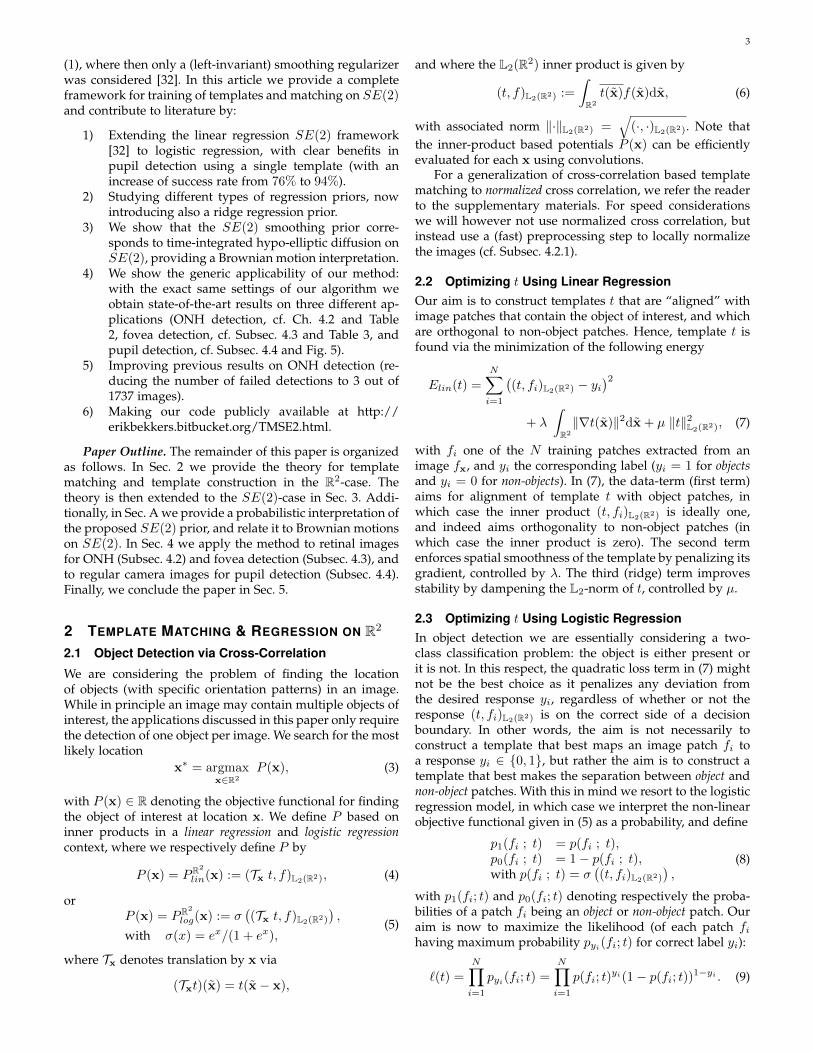
Fig. 1. A retinal image f of the optic nerve head and a volume renderingof the orientation score Uf (obtained via a wavelet transformWψ).

orientations, and provides a comprehensive decompositionof an image based on local orientations, see Fig. 1 and 2.Cross-correlation based template matching is then definedvia L2 inner-products of a template T ∈ L2(SE(2)) and anorientation score Uf ∈ L2(SE(2)). In this paper, we learntemplates T by means of generalized linear regression.

In the R2-case (which we later extend to orientationscores, the SE(2)-case), we define templates t ∈ L2(R2) viathe optimization of energy functionals of the form

t∗ = argmint∈L2(R2)

E(t) := S(t) +R(t) , (1)

where the energy functional E(t) consists of a data termS(t), and a regularization term R(t). Since the templatesoptimized in this form are used in a linear cross-correlationbased framework, we will use inner products in S, in whichcase (1) can be regarded as a generalized linear regressionproblem with a regularization term. For example, (1) be-comes a regression problem generally known under the

arX

iv:1

603.

0330

4v5

[cs

.CV

] 9

Mar

201

7

2

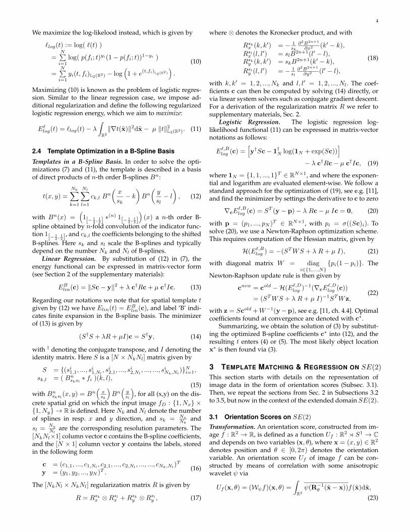
Fig. 2. In orientation scores Uf , constructed from an image f via the ori-entation score transformWψ , we make use of a left-invariant derivativeframe ∂ξ, ∂η , ∂θ that is aligned with the orientation θ corresponding toeach layer in the score. Three slices and the corresponding left-invariantframes are shown separately (at θ ∈ 0, π

4, 3π

4).

name ridge regression [8], when taking

S(t) =N∑i=1

((t, fi)L2(R2) − yi

)2, and R(t) = µ‖t‖2L2(R2),

where fi is one of N image patches, yi ∈ 0, 1 is thecorresponding desired filter response, and where µ is aparameter weighting the regularization term. The regressionis then from an input image patch fi to a desired responseyi, and the template t can be regarded as the “set of weights”that are optimized in the regression problem. In this articlewe consider both quadratic (linear regression) and logistic(logistic regression) losses in S. For regularization we con-sider terms of the form

R(t) = λ

∫R2

‖∇t(x)‖2dx + µ‖t‖2L2(R2),

and thus combine the classical ridge regression with asmoothing term (weighted by λ).

In our extension of smoothed regression to orientationscores we employ similar techniques. However, here wemust recognize a curved geometry on the domain R2 o S1,which we identify with the group of roto-translations: theLie group SE(2) equipped with group product

g · g′ = (x, θ) · (x′, θ′) = (Rθx′ + x, θ + θ′). (2)

In this product the orientation θ influences the product onthe spatial part. Therefore we write R2 o S1 instead ofR2 × S1, as it is a semi-direct group product (and not adirect product). Accordingly, we must work with a rotatingderivative frame (instead of axis aligned derivatives) thatis aligned with the group elements (x, θ) ∈ SE(2), see e.g.the (∂ξ, ∂η, ∂θ)-frames in Fig. 2. This derivative frame allowsfor (anisotropic) smoothing along oriented structures. As wewill show in this article (Sec. A), the proposed smoothingscheme has the probabilistic interpretation of time inte-grated Brownian motion on SE(2) [9], [10].

Regression and Group Theory. Regularization in (gener-alized) linear regression generally leads to more robust clas-sifiers/regressions, especially when a low number of train-ing samples are available. Different types of regularizationsin regression problems have been intensively studied in e.g.[11], [12], [13], [14], [15], and the choice for regularization-type depends on the problem: E.g. L1-type regularization isoften used to sparsify the regression weights, whereas L2-type regularization is more generally used to prevent over-fitting by penalizing outliers (e.g. in ridge regression [8]).

Smoothing of regression coefficients by penalizing the L2-norm of the derivative along the coefficients is less common,but it can have a significant effect on performance [13], [16].

We solve problem (1) in the context of smoothing splines:We discretize the problem by expanding the templates ina finite B-spline basis, and optimize over the spline co-efficients. For d-dimensional Euclidean spaces, smoothingsplines have been well studied [17], [18], [19], [20]. In thispaper, we extend the concept to the curved space SE(2) andprovide explicit forms of the discrete regularization matri-ces. Furthermore, we show that the extended framework canbe used for time integrated Brownian motions on SE(2),and show near to perfect comparisons to the exact solutionsfound in [9], [10].

In general, statistics and regression on Riemannian man-ifolds are powerful tools in medical imaging and computervision [21], [22], [23], [24]. More specifically in patternmatching and registration problems Lie groups are oftenused to describe deformations. E.g. in [25] the authorslearn a regression function Rm → A(2) from a discrete m-dimensional feature vector to a deformation in the affinegroup A(2). Their purpose is object tracking in video se-quences. This work is however not concerned with de-formation analysis, we instead learn a regression functionL2(SE(2)) → R from continuous densities on the Liegroup SE(2) (obtained via an invertible orientation scoretransform) to a desired filter response. Our purpose isobject detection in 2D images. In our regression we imposesmoothed regression with a time-integrated hypo-ellipticBrownian motion prior and thereby extend least squaresregression to smoothed regression on SE(2) involving firstorder variation in Sobolev-type of norms.

Application Area of the Proposed Method. The strengthof our approach is demonstrated with the application toanatomical landmark detection in medical retinal imagesand pupil localization in regular camera images. In theretinal application we consider the problem of detecting theoptic nerve head (ONH) and the fovea. Many image analysisapplications require the robust, accurate and fast detectionof these structures, see e.g. [26], [27], [28], [29]. In all threedetection problems the objects of interest are characterizedby (surrounding) curvilinear structures (blood vessels in theretina; eyebrow, eyelid, pupil and other contours for pupildetection), which are conveniently represented in invertibleorientation scores. The invertibility condition implies that allimage data is contained in the orientation score [30] [7]. Withthe proposed method we achieve state-of-the-art resultsboth in terms of detection performance and speed: highdetection performance is achieved by learning templatesthat make optimal use of the line patterns in orientationscores; speed is achieved by a simple, yet effective, cross-correlation template matching approach.

Contribution of this Work. This article builds upontwo published conference papers [31], [32]. In the first wedemonstrated that high detection performance could beachieved by considering cross-correlation based templatematching in SE(2), using only handcrafted templates andwith the application of ONH detection in retinal images [31].In the second we then showed on the same application thatbetter performance could be achieved by training templatesusing the optimization of energy functionals of the form of

3

(1), where then only a (left-invariant) smoothing regularizerwas considered [32]. In this article we provide a completeframework for training of templates and matching on SE(2)and contribute to literature by:

1) Extending the linear regression SE(2) framework[32] to logistic regression, with clear benefits inpupil detection using a single template (with anincrease of success rate from 76% to 94%).

2) Studying different types of regression priors, nowintroducing also a ridge regression prior.

3) We show that the SE(2) smoothing prior corre-sponds to time-integrated hypo-elliptic diffusion onSE(2), providing a Brownian motion interpretation.

4) We show the generic applicability of our method:with the exact same settings of our algorithm weobtain state-of-the-art results on three different ap-plications (ONH detection, cf. Ch. 4.2 and Table2, fovea detection, cf. Subsec. 4.3 and Table 3, andpupil detection, cf. Subsec. 4.4 and Fig. 5).

5) Improving previous results on ONH detection (re-ducing the number of failed detections to 3 out of1737 images).

6) Making our code publicly available at http://erikbekkers.bitbucket.org/TMSE2.html.

Paper Outline. The remainder of this paper is organizedas follows. In Sec. 2 we provide the theory for templatematching and template construction in the R2-case. Thetheory is then extended to the SE(2)-case in Sec. 3. Addi-tionally, in Sec. A we provide a probabilistic interpretation ofthe proposed SE(2) prior, and relate it to Brownian motionson SE(2). In Sec. 4 we apply the method to retinal imagesfor ONH (Subsec. 4.2) and fovea detection (Subsec. 4.3), andto regular camera images for pupil detection (Subsec. 4.4).Finally, we conclude the paper in Sec. 5.

2 TEMPLATE MATCHING & REGRESSION ON R2

2.1 Object Detection via Cross-Correlation

We are considering the problem of finding the locationof objects (with specific orientation patterns) in an image.While in principle an image may contain multiple objects ofinterest, the applications discussed in this paper only requirethe detection of one object per image. We search for the mostlikely location

x∗ = argmaxx∈R2

P (x), (3)

with P (x) ∈ R denoting the objective functional for findingthe object of interest at location x. We define P based oninner products in a linear regression and logistic regressioncontext, where we respectively define P by

P (x) = PR2

lin(x) := (Tx t, f)L2(R2), (4)

orP (x) = PR2

log(x) := σ((Tx t, f)L2(R2)

),

with σ(x) = ex/(1 + ex),(5)

where Tx denotes translation by x via

(Txt)(x) = t(x− x),

and where the L2(R2) inner product is given by

(t, f)L2(R2) :=

∫R2

t(x)f(x)dx, (6)

with associated norm ‖·‖L2(R2) =√

(·, ·)L2(R2). Note thatthe inner-product based potentials P (x) can be efficientlyevaluated for each x using convolutions.

For a generalization of cross-correlation based templatematching to normalized cross correlation, we refer the readerto the supplementary materials. For speed considerationswe will however not use normalized cross correlation, butinstead use a (fast) preprocessing step to locally normalizethe images (cf. Subsec. 4.2.1).

2.2 Optimizing t Using Linear RegressionOur aim is to construct templates t that are “aligned” withimage patches that contain the object of interest, and whichare orthogonal to non-object patches. Hence, template t isfound via the minimization of the following energy

Elin(t) =N∑i=1

((t, fi)L2(R2) − yi

)2+ λ

∫R2

‖∇t(x)‖2dx + µ ‖t‖2L2(R2), (7)

with fi one of the N training patches extracted from animage fx, and yi the corresponding label (yi = 1 for objectsand yi = 0 for non-objects). In (7), the data-term (first term)aims for alignment of template t with object patches, inwhich case the inner product (t, fi)L2(R2) is ideally one,and indeed aims orthogonality to non-object patches (inwhich case the inner product is zero). The second termenforces spatial smoothness of the template by penalizing itsgradient, controlled by λ. The third (ridge) term improvesstability by dampening the L2-norm of t, controlled by µ.

2.3 Optimizing t Using Logistic RegressionIn object detection we are essentially considering a two-class classification problem: the object is either present orit is not. In this respect, the quadratic loss term in (7) mightnot be the best choice as it penalizes any deviation fromthe desired response yi, regardless of whether or not theresponse (t, fi)L2(R2) is on the correct side of a decisionboundary. In other words, the aim is not necessarily toconstruct a template that best maps an image patch fi toa response yi ∈ 0, 1, but rather the aim is to construct atemplate that best makes the separation between object andnon-object patches. With this in mind we resort to the logisticregression model, in which case we interpret the non-linearobjective functional given in (5) as a probability, and define

p1(fi ; t) = p(fi ; t),p0(fi ; t) = 1− p(fi ; t),with p(fi ; t) = σ

((t, fi)L2(R2)

),

(8)

with p1(fi; t) and p0(fi; t) denoting respectively the proba-bilities of a patch fi being an object or non-object patch. Ouraim is now to maximize the likelihood (of each patch fihaving maximum probability pyi(fi; t) for correct label yi):

`(t) =N∏i=1

pyi(fi; t) =N∏i=1

p(fi; t)yi(1− p(fi; t))1−yi . (9)

4

We maximize the log-likelood instead, which is given by

`log(t) := log( `(t) )

=N∑i=1

log( p(fi; t)yi(1− p(fi; t))1−yi )

=N∑i=1

yi(t, fi)L2(R2) − log(

1 + e(t,fi)L2(R2)

).

(10)

Maximizing (10) is known as the problem of logistic regres-sion. Similar to the linear regression case, we impose ad-ditional regularization and define the following regularizedlogistic regression energy, which we aim to maximize:

E`log(t) = `log(t)− λ∫R2

‖∇t(x)‖2dx− µ ‖t‖2L2(R2). (11)

2.4 Template Optimization in a B-Spline Basis

Templates in a B-Spline Basis. In order to solve the opti-mizations (7) and (11), the template is described in a basisof direct products of n-th order B-splines Bn:

t(x, y) =Nk∑k=1

Nl∑l=1

ck,l Bn

(x

sk− k

)Bn(y

sl− l), (12)

with Bn(x) =(

1[− 12 ,

12 ] ∗

(n) 1[− 12 ,

12 ]

)(x) a n-th order B-

spline obtained by n-fold convolution of the indicator func-tion 1[− 1

2 ,12 ], and ck,l the coefficients belonging to the shifted

B-splines. Here sk and sl scale the B-splines and typicallydepend on the number Nk and Nl of B-splines.

Linear Regression. By substitution of (12) in (7), theenergy functional can be expressed in matrix-vector form(see Section 2 of the supplementary materials):

EBlin(c) = ‖Sc− y‖2 + λ c†Rc + µ c†Ic. (13)

Regarding our notations we note that for spatial template tgiven by (12) we have Elin(t) = EBlin(c), and label ‘B’ indi-cates finite expansion in the B-spline basis. The minimizerof (13) is given by

(S†S + λR+ µI)c = S†y, (14)

with † denoting the conjugate transpose, and I denoting theidentity matrix. Here S is a [N ×NkNl] matrix given by

S = (si1,1, ..., si1,Nl, si2,1, ..., s

i2,Nl

, ..., ..., siNk,Nl)Ni=1,

sk,l = ( Bnsksl ∗ fi )(k, l),(15)

with Bnsksl(x, y) = Bn(xsk

)Bn(ysl

), for all (x,y) on the dis-

crete spatial grid on which the input image fD : 1, Nx ×1, Ny → R is defined. Here Nk and Nl denote the numberof splines in resp. x and y direction, and sk = Nx

Nkand

sl =Ny

Nlare the corresponding resolution parameters. The

[NkNl×1] column vector c contains the B-spline coefficients,and the [N × 1] column vector y contains the labels, storedin the following form

c = (c1,1, ..., c1,Nl, c2,1, ..., c2,Nl

, ..., ..., cNk,Nl)T

y = (y1, y2, ..., yN )T .(16)

The [NkNl ×NkNl] regularization matrix R is given by

R = Rskx ⊗Rslx +Rsky ⊗Rsly , (17)

where ⊗ denotes the Kronecker product, and with

Rskx (k, k′) = − 1sk∂2B2n+1

∂x2 (k′ − k),

Rslx (l, l′) = slB2n+1(l′ − l),

Rsky (k, k′) = skB2n+1(k′ − k),

Rsly (l, l′) = − 1sl∂2B2n+1

∂y2 (l′ − l),

(18)

with k, k′ = 1, 2, ..., Nk and l, l′ = 1, 2, ..., Nl. The coef-ficients c can then be computed by solving (14) directly, orvia linear system solvers such as conjugate gradient descent.For a derivation of the regularization matrix R we refer tosupplementary materials, Sec. 2.

Logistic Regression. The logistic regression log-likelihood functional (11) can be expressed in matrix-vectornotations as follows:

E`,Blog (c) =[y†Sc− 1†N log(1N + exp(Sc))

]− λ c†Rc− µ c†Ic, (19)

where 1N = 1, 1, ..., 1T ∈ RN×1, and where the exponen-tial and logarithm are evaluated element-wise. We follow astandard approach for the optimization of (19), see e.g. [11],and find the minimizer by settings the derivative to c to zero

∇cE`,Blog (c) = ST (y − p)− λ Rc− µ Ic = 0, (20)

with p = (p1, ..., pN )T ∈ RN×1, with pi = σ((Sc)i). Tosolve (20), we use a Newton-Raphson optimization scheme.This requires computation of the Hessian matrix, given by

H(E`,Blog ) = −(STWS + λ R+ µ I), (21)

with diagonal matrix W = diagi∈1,...,N

pi(1− pi). The

Newton-Raphson update rule is then given by

cnew = cold −H(E`,Dlog )−1(∇cE`,Dlog (c))

= (STWS + λ R+ µ I)−1STWz,(22)

with z = Scold +W−1(y−p), see e.g. [11, ch. 4.4]. Optimalcoefficients found at convergence are denoted with c∗.

Summarizing, we obtain the solution of (3) by substitut-ing the optimized B-spline coefficients c∗ into (12), and theresulting t enters (4) or (5). The most likely object locationx∗ is then found via (3).

3 TEMPLATE MATCHING & REGRESSION ON SE(2)

This section starts with details on the representation ofimage data in the form of orientation scores (Subsec. 3.1).Then, we repeat the sections from Sec. 2 in Subsections 3.2to 3.5, but now in the context of the extended domain SE(2).

3.1 Orientation Scores on SE(2)

Transformation. An orientation score, constructed from im-age f : R2 → R, is defined as a function Uf : R2 o S1 → Cand depends on two variables (x, θ), where x = (x, y) ∈ R2

denotes position and θ ∈ [0, 2π) denotes the orientationvariable. An orientation score Uf of image f can be con-structed by means of correlation with some anisotropicwavelet ψ via

Uf (x, θ) = (Wψf)(x, θ) =

∫R2

ψ(R−1θ (x− x))f(x)dx,

(23)

5

where ψ ∈ L2(R2) is the correlation kernel, aligned withthe x-axis, where Wψ denotes the transformation betweenimage f and orientation score Uf , ψθ(x) = ψ(R−1

θ x), andRθ is a counter clockwise rotation over angle θ.

In this work we choose cake wavelets [6], [7] for ψ. Whilein general any kind of anisotropic wavelet could be used tolift the image to SE(2), cake wavelets ensure that no data-evidence is lost during the transformation: By design theset of all rotated wavelets uniformly cover the full Fourierdomain of disk-limited functions with zero mean, and havethereby the advantage over other oriented wavelets (s.a.Gabor wavelets for specific scales) that they capture allscales and allow for a stable inverse transformation W∗ψfrom the score back to the image [6], [10].

Left-Invariant Derivatives. The domain of an orienta-tion score is essentially the classical Euclidean motion groupSE(2) of planar translations and rotations, and is equippedwith group product g·g′ = (x, θ)·(x′, θ′) = (Rθx

′+x, θ+θ′).Here, we can recognize a curved geometry (cf. Fig. 2), andit is therefore useful to work in rotating frame of reference.As such, we use the left invariant derivative frame [9], [10]:

∂ξ := cos θ ∂x + sin θ ∂y, ∂η := − sin θ ∂x + cos θ ∂y, ∂θ .(24)

Using this derivative frame we will construct in Subsec. 3.3a regularization term in which we can control the amountof (anisotropic) smoothness along line structures.

3.2 Object Detection via Cross-CorrelationAs in Section 2, we search for the most likely object locationx∗ via (3), but now we define functional P respectively forthe linear and logistic regression case in SE(2) by1:

P (x) = PSE(2)lin (x) :=(Tx T, |Uf |)L2(SE(2)), or (25)

P (x) = PSE(2)log (x) :=σ

((Tx T, |Uf |)L2(SE(2))

), (26)

with (TxT )(x, θ) = T (x−x, θ). The L2(SE(2))-inner prod-uct is defined by

(T, |Uf |)L2(SE(2)) :=

∫R2

∫ 2π

0T (x, θ) |Uf | (x, θ)dxdθ, (27)

with norm ‖·‖L2(SE(2)) =√

(·, ·)L2(SE(2)).

3.3 Optimizing T Using Linear RegressionFollowing the same reasoning as in Section 2.2 we search forthe template that minimizes

Elin(T ) =N∑i=1

((T, |Ufi |)L2(SE(2)) − yi

)2+ λ

∫R2

∫ 2π

0‖∇T (x, θ)‖2Ddxdθ + µ‖T‖2L2(SE(2)), (28)

with smoothing term:

‖∇T (g)‖2D = Dξξ

∣∣∣∣∂T∂ξ (g)

∣∣∣∣2+Dηη

∣∣∣∣∂T∂η (g)

∣∣∣∣2+Dθθ

∣∣∣∣∂T∂θ (g)

∣∣∣∣2 .(29)

1. Since both the inner product and the construction of orientationscores Uf from images f are linear, template matching might as well beperformed directly on the 2D images (likewise (4) and (5)). Hence, herewe take the modulus of the score as a non-linear intermediate step [32].

Here,∇T = (∂T∂ξ ,∂T∂η ,

∂T∂θ )T denotes the left-invariant gradi-

ent. Note that ∂ξ gives the spatial derivative in the directionaligned with the orientation score kernel used at layer θ,recall Fig. 2. The parameters Dξξ , Dηη and Dθθ ≥ 0 are thenused to balance the regularization in the three directions.Similar to this problem, first order Tikhonov-regularizationon SE(2) is related, via temporal Laplace transforms, toleft–invariant diffusions on the group SE(2) (Sec. A), inwhich case Dξξ , Dηη and Dθθ denote the diffusion constantsin ξ, η and θ direction. Here we set Dξξ = 1, Dηη = 0,and thereby we get Laplace transforms of hypo-ellipticdiffusion processes [10], [33]. Parameter Dθθ can be usedto tune between isotropic (large Dθθ) and anisotropic (lowDθθ) diffusion (see e.g. [32, Fig. 3]). Note that anisotropicdiffusion, via a low Dθθ, is preferred as we want to maintainline structures in orientation scores.

3.4 Optimizing T Using Logistic RegressionSimilarly to what is done in Subsec. 2.3 we can change thequadratic loss of (28) to a logistic loss, yielding the followingenergy functional

Elog(T ) = Llog(T )− λ∫R2

∫ 2π

0‖∇T (x, θ)‖2Ddxdθ

− µ‖T‖2L2(SE(2)), (30)

with log-likelihood (akin to (10) for the R2 case)

Llog(T ) =N∑i=1

yi(T, |Ufi |)L2(SE(2))

− log(

1 + e(T,|Ufi |)L2(SE(2))

).

(31)

The optimization of (28) and (30) follows quite closely theprocedure as described in Sec. 2 for the 2D case. In fact,when T is expanded in a B-spline basis, the exact samematrix-vector formulation can be used.

3.5 Template Optimization in a B-Spline BasisTemplates in a B-Spline Basis. The template T is expandedin a B-spline basis as follows

T (x, y, θ) =Nk∑k=1

Nl∑l=1

Nm∑m=1

ck,l,m·

Bn(xsk− k

)Bn(ysl− l)Bn(θmod 2π

sm−m

),

(32)

with Nk, Nl and Nm the number of B-splines in respectivelythe x, y and θ direction, ck,l,m the corresponding basis coeffi-cients, and with angular resolution parameter sm = 2π/Nm.

Linear Regression. The shape of the minimizer of energyfunctional Elin(T ) in the SE(2) case is the same as forElin(t) in the R2 case, and is again of the form given in (13).However, now the definitions of S, R and c are different.Now, S is a [N ×NkNlNm] matrix given by

S = (si1,1,1, ..., si1,1,Nm, ..., s1,Nl,Nm

, ..., siNk,Nl,Nm)Ni=1,

sk,l,m = ( Bnskslsm ∗ Ufi )(k, l,m),(33)

with Bnskslsm(x, y, θ) = Bn(xsk

)Bn(ysl

)Bn(θ mod 2π

sm

).

Vector c is a [NkNlNm × 1] column vector containing theB-spline coefficients and is stored as follows:

c = (c1,1,1, ..., c1,1,Nm , ..., c1,Nl,Nm , ..., cNk,Nl,Nm)T . (34)

6

The explicit expression and the derivation of [NkNlNm ×NkNlNm] matrixR, which encodes the left invariant deriva-tives, can be found in the supplementary materials Sec. 2.

Logistic Regression Also for the logistic regression casewe optimize energy functional (30) in the same form as (11)in the R2 case, by using the corresponding expressions forS, R, and c in Eq. (19). These expressions can be insertedin the functional (19) and again the same techniques (aspresented in Subsection 2.4) can be used to minimize thiscost on SE(2).

3.6 Probabilistic Interpretation of the SE(2) SmoothingPrior

In this section we only provide a brief introduction to theprobabilistic interpretation of the SE(2) smoothing prior,and refer the interested reader to the supplementary materi-als for full details. Consider the classic approach to noisesuppression in images via diffusion regularizations withPDE’s of the form

∂∂τ u = ∆u,u|τ=0 = u0,

(35)

where ∆ denotes the Laplace operator. Solving (40) for anydiffusion time τ > 0 gives a smoothed version of the inputu0. The time-resolvent process of the PDE is defined by theLaplace transform with respect to τ ; time τ is integratedout using a memoryless negative exponential distributionP (T = τ) = αe−ατ . Then, the time integrated solutions

t(x) = α

∫ ∞0

u(x, τ)e−ατdτ,

with decay parameter α, are in fact the solutions [34]

t = argmint∈L2(R2)

[‖t− t0‖2L2(R2) + λ

∫R2

‖∇t(x)‖2 dx

], (36)

with λ = α−1. Such time integrated diffusions (Eq. (36)) canalso be obtained by optimization of the linear regressionfunctionals given by Eq. (7) and Eq. (25) for the R2 andSE(2) case respectively.

In the supplementary materials we establish this con-nection for the SE(2) case, and show how the smoothingregularizer in (28) and (30) relates to Laplace transforms ofhypo-elliptic diffusions on the group SE(2) [9], [10]. Moreprecisely, we formulate a special case of our problem (thesingle patch problem) which involves only a single trainingsample Uf1 , and show in a formal theorem that the solutionis up to scalar multiplication the same as the resolvent hypo-elliptic diffusion kernel. The underlying probabilistic inter-pretation is that of Brownian motions on SE(2), where theresolvent hypo-elliptic diffusion kernel gives a probabilitydensity of finding a random brush stroke at location x withorientation θ, given that a ‘drunkman’s pencil’ starts at theorigin at time zero.

In the supplementary materials we demonstrate the highaccuracy of our discrete numeric regression method usingB-spline expansions with near to perfect comparisons tothe continuous exact solutions of the single patch problem.In fact, we have established an efficient B-spline finite ele-ment implementation of hypo-elliptic Brownian motions onSE(2), in addition to other numerical approaches in [9].

4 APPLICATIONS

Our applications of interest are in retinal image analysis. Inthis section we establish and validate an algorithm pipelinefor the detection of the optic nerve head (Subsec. 4.2) andfovea (Subsec. 4.3) in retinal images, and the pupil (Sub-sec. 4.4) in regular camera images. Before we proceed tothe application sections, we first describe the experimentalset-up (Subsec. 4.1). All experiments discussed in this sec-tion are reproducible; the data (with annotations) as wellas the full code (Wolfram Mathematica notebooks) used inthe experiments are made available at: http://erikbekkers.bitbucket.org/TMSE2.html. In the upcoming sections weonly report the most relevant experimental results. Moredetails on each application (examples of training samples,implementation details, a discussion on parameter settings,computation times, and examples of successful/failed de-tections) are provided in the supplementary materials.

4.1 The experimental set-upTemplates. In our experiments we compare the performanceof different template types, which we label as follows:

A: Templates obtained by taking the average of all posi-tive patches (yi = 1) in the training set, then normal-ized to zero mean and unit standard deviation.

B: Templates optimized without any regularization.C : Templates optimized with an optimal µ, and with

λ = 0.D: Templates optimized with an optimal λ and with µ =

0.E: Templates optimized with optimal µ and λ.

The trained templates (B-E) are obtained either via linear orlogistic regression in the R2 setting (see Subsec. 2.4 and Sub-sec. 2.4), or in the SE(2) setting (see Subsec. 3.5 and Subsec.3.5). In both the R2 and SE(2) case, linear regression basedtemplates are indicated with subscript lin, and logistic re-gression based templates with log . Optimality of parametervalues is defined using generalized cross validation (GCV),which we soon explain in this section. We generally foundthat (via optimization using GCV) the optimal settings fortemplate E were µ ≈ 0.5µ∗, and λ ≈ 0.5λ∗, with µ∗ and λ∗

respectively the optimal parameters for template C and D.Matching with Multiple Templates. When performing

template matching, we use Eq. (4) and Eq. (25) for re-spectively the R2 and SE(2) case for templates obtainedvia linear regression and for template A. For templatesobtained via logistic regression we use respectively Eq. (5)and Eq. (26). When we combine multiple templates wesimply add the objective functionals. E.g, when combiningtemplate Clin:R2 and Dlog:SE(2) we solve the problem

x∗ = argmaxx∈R2

PR2

Clin(x) + P

SE(2)Dlog

(x),

where PR2

Clin(x) is the objective functional (see Eq. (4)) ob-

tained with template Clin:R2 , and PSE(2)Dlog

(x) (see Eq. (26)) isobtained with template Dlog:SE(2).

Rotation and Scale Invariance. The proposed templatematching scheme can adapted for rotation-scale invariantmatching, this is discussed in Sec. 5 of the supplementarymaterials. For a generic object recognition task, however,

7

global rotation or scale invariance are not necessarily de-sired properties. Datasets often contain objects in a hu-man environment context, in which some objects tend toappear in specific orientations (e.g. eye-brows are oftenhorizontal above the eye and vascular trees in the retinadepart the ONH typically along a vertical axis). Discardingsuch knowledge by introducing rotation/scale invariance islikely to have an adversary effect on the performance, whileincreasing computational load. In Sec. 5 of the supplemen-tary materials we tested a rotation/scale invariant adapta-tion of our method and show that in the three discussedapplications this did indeed not lead to improved results,but in fact worsened the results slightly.

Automatic Parameter Selection via Generalized CrossValidation. An ideal template generalizes well to new datasamples, meaning that it has low prediction error on in-dependent data samples. One method to predict how wellthe system generalizes to new data is via generalized crossvalidation (GCV), which is essentially an approximation ofleave-one-out cross validation [35]. The vector containingall predictions is given by y = Scµ,λ, in which we cansubstitute the solution for cµ,λ (from Eq. (14)) to obtain

y = Aµ,λy, with

Aµ,λ = S(S†S + λR+ µI)−1S†,(37)

where Aµ,λ is the so-called smoother matrix. Then the gener-alized cross validation value [35] is defined as

GCV (µ, λ) ≡1N ‖Ω(I −Aµ,λ)y‖2

(1− trace(Aµ,λ)/N)2 . (38)

In the retinal imaging applications we set Ω = I . In thepupil detection application we set Ω = diag

i∈1,...,Nyi. As

such, we do not penalize errors on negative samples as herethe diversity of negative patches is too large for parameteroptimization via GCV. Parameter settings are consideredoptimal when they minimize the GCV value.

In literature various extensions of GCV are proposedfor generalized linear models [36], [37], [38]. For logisticregression we use the approach by O’Sullivan et al. [36]: weiterate the Newton-Raphson algorithm until convergence,then, at the final iteration we compute the GCV value onthe quadratic approximation (Eq. (22)).

Success Rates. Performance of the templates is evaluatedusing success rates. The success rate of a template is the per-centage of images in which the target object was successfullylocalized. In both optic nerve head (Subsec. 4.2) and fovea(Subsec. 4.3) detection experiments, a successful detectionis defined as such if the detected location x∗ (Eq. (3)) lieswithin one optic disk radius distance to the actual location.For pupil detection both the left and right eye need to bedetected and we therefore use the following normalizederror metric

e =max(dleft, dright)

w, (39)

in which w is the (ground truth) distance between the leftand right eye, and dleft and dright are respectively thedistances of detection locations to the left and right eye.

k-Fold Cross Validation. For correct unbiased evalua-tion, none of the test images are used for training of thetemplates, nor are they used for parameter optimization.

We perform k-fold cross validation: The complete dataset israndomly partitioned into k subsets. Training (patch extrac-tion, parameter optimization and template construction) isdone using the data from k − 1 subsets. Template matchingis then performed on the remaining subset. This is donefor all k configurations with k − 1 training subsets and onetest subset, allowing us to compute the average performance(success rate) and standard deviation. We set k = 5.

4.2 Optic Nerve Head Detection in Retinal ImagesOur first application to retinal images is optic nerve headdetection. The ONH is one of the key anatomical landmarksin the retina, and its location is often used as a referencepoint to define regions of interest for the analysis of theretina. The detection hereof is therefore an essential step inmany automated retinal image analysis pipelines.

The ONH has two main characteristics: 1) it often ap-pears as a bright disk-like structure on color fundus (CF)images (dark on SLO images), and 2) it is the place fromwhich blood vessels leave the retina. Traditionally, methodshave mainly focused on the first characteristic [39], [40],[41]. However, in case of bad contrast of the optic disk,or in the presence of pathology (especially bright lesions,see e.g. Fig. 3), these methods typically fail. Most of therecent ONH detection methods therefore also include thevessel patterns in the analysis; either via explicit vesselsegmentation [42], [43], vessel density measures [44], [45],or via additional orientation pattern matching steps [46]. Inour method, both the appearance and vessel characteristicsare addressed in an efficient integrated template matchingapproach, resulting in state-of-the-art performance both interms of success rates and computation time. We targetthe first characteristic with template matching on R2. Thesecond is targeted with template matching on SE(2).

4.2.1 Processing Pipeline & DataProcessing Pipeline. First, the images are rescaled to aworking resolution of 40 µm/pix. In our experiments theaverage resolution per dataset was determined using theaverage optic disk diameter (which is on average 1.84mm).The images are normalized for contrast and illuminationvariations using the method from [47]. Finally, in order toput more emphasis on contextual/shape information, ratherthan pixel intensities, we apply a soft binarization to thelocally normalized (cf. Eq. (31) in Ch. 3 of the supplementarymaterials) image f via the mapping erf(8f).

For the orientation score transform we use Nθ = 12uniformly sampled orientations from 0 to π and lift theimage using cake wavelets [6], [7]. For phase-invariant,nonlinear, left-invariant [10], and contractive [48] processingon SE(2), we work with the modulus of the complex val-ued orientation scores rather than with the complex-valuedscores themselves (taking the modulus of quadrature filterresponses is an effective technique for line detection, see e.g.Freeman et al. [49]).

Due to differences in image characteristics, training andmatching is done separately for the SLO and the colorfundus images. For SLO images we use the near infraredchannel, for RGB fundus images we use the green channel.

Positive training samples fi are defined as Nx × Nypatches, with Nx = Ny = 251, centered around true ONH

8

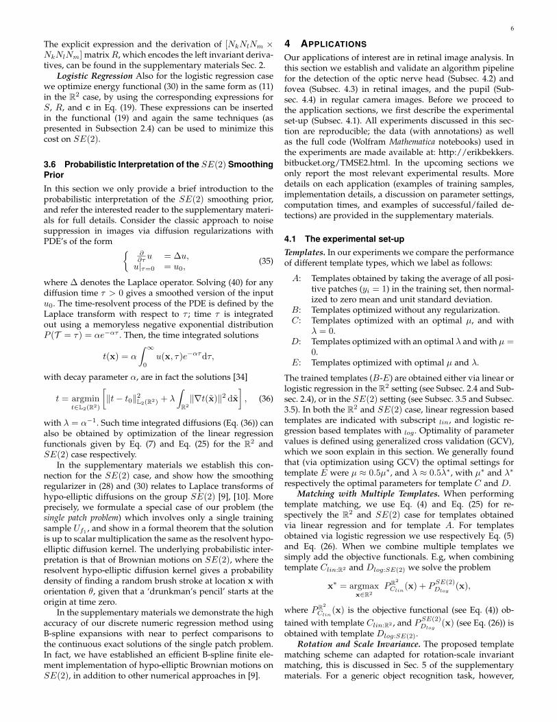
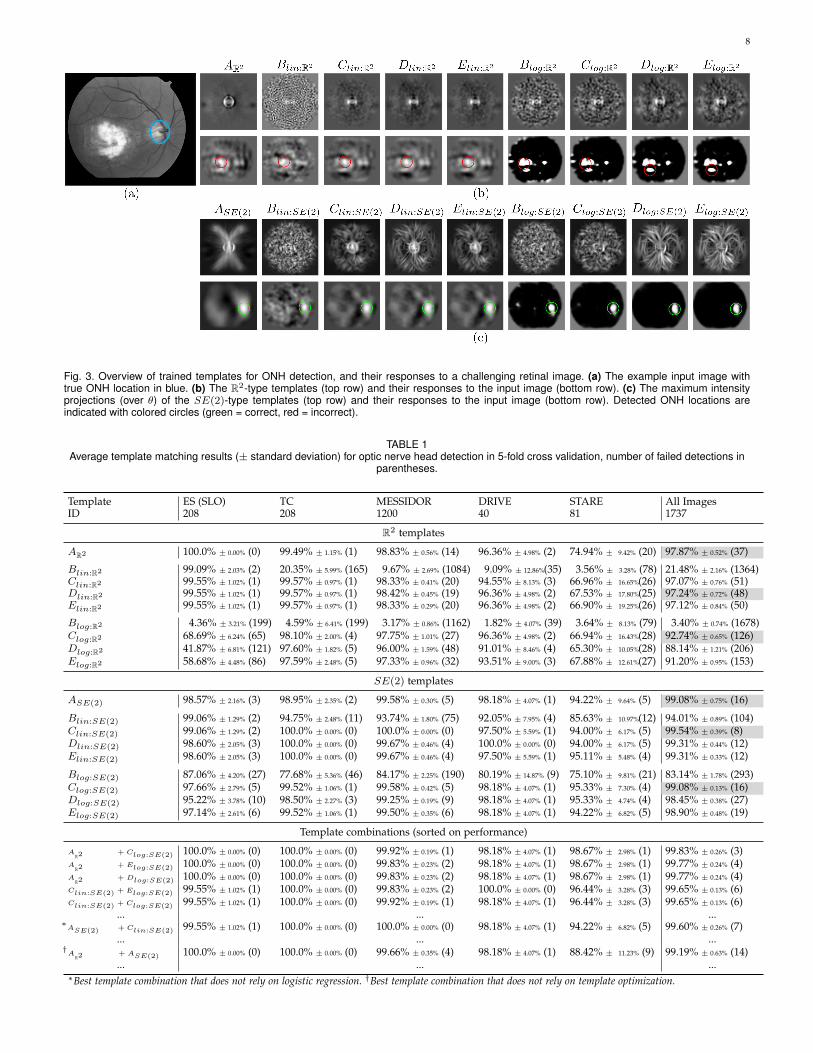
Fig. 3. Overview of trained templates for ONH detection, and their responses to a challenging retinal image. (a) The example input image withtrue ONH location in blue. (b) The R2-type templates (top row) and their responses to the input image (bottom row). (c) The maximum intensityprojections (over θ) of the SE(2)-type templates (top row) and their responses to the input image (bottom row). Detected ONH locations areindicated with colored circles (green = correct, red = incorrect).

TABLE 1Average template matching results (± standard deviation) for optic nerve head detection in 5-fold cross validation, number of failed detections in

parentheses.

Template ES (SLO) TC MESSIDOR DRIVE STARE All ImagesID 208 208 1200 40 81 1737

R2 templates

AR2 100.0% ± 0.00% (0) 99.49% ± 1.15% (1) 98.83% ± 0.56% (14) 96.36% ± 4.98% (2) 74.94% ± 9.42% (20) 97.87% ± 0.52% (37)

Blin:R2 99.09% ± 2.03% (2) 20.35% ± 5.99% (165) 9.67% ± 2.69% (1084) 9.09% ± 12.86%(35) 3.56% ± 3.28% (78) 21.48% ± 2.16% (1364)Clin:R2 99.55% ± 1.02% (1) 99.57% ± 0.97% (1) 98.33% ± 0.41% (20) 94.55% ± 8.13% (3) 66.96% ± 16.65%(26) 97.07% ± 0.76% (51)Dlin:R2 99.55% ± 1.02% (1) 99.57% ± 0.97% (1) 98.42% ± 0.45% (19) 96.36% ± 4.98% (2) 67.53% ± 17.80%(25) 97.24% ± 0.72% (48)Elin:R2 99.55% ± 1.02% (1) 99.57% ± 0.97% (1) 98.33% ± 0.29% (20) 96.36% ± 4.98% (2) 66.90% ± 19.25%(26) 97.12% ± 0.84% (50)

Blog:R2 4.36% ± 3.21% (199) 4.59% ± 6.41% (199) 3.17% ± 0.86% (1162) 1.82% ± 4.07% (39) 3.64% ± 8.13% (79) 3.40% ± 0.74% (1678)Clog:R2 68.69% ± 6.24% (65) 98.10% ± 2.00% (4) 97.75% ± 1.01% (27) 96.36% ± 4.98% (2) 66.94% ± 16.43%(28) 92.74% ± 0.65% (126)Dlog:R2 41.87% ± 6.81% (121) 97.60% ± 1.82% (5) 96.00% ± 1.59% (48) 91.01% ± 8.46% (4) 65.30% ± 10.05%(28) 88.14% ± 1.21% (206)Elog:R2 58.68% ± 4.48% (86) 97.59% ± 2.48% (5) 97.33% ± 0.96% (32) 93.51% ± 9.00% (3) 67.88% ± 12.61%(27) 91.20% ± 0.95% (153)

SE(2) templates

ASE(2) 98.57% ± 2.16% (3) 98.95% ± 2.35% (2) 99.58% ± 0.30% (5) 98.18% ± 4.07% (1) 94.22% ± 9.64% (5) 99.08% ± 0.75% (16)

Blin:SE(2) 99.06% ± 1.29% (2) 94.75% ± 2.48% (11) 93.74% ± 1.80% (75) 92.05% ± 7.95% (4) 85.63% ± 10.97%(12) 94.01% ± 0.89% (104)Clin:SE(2) 99.06% ± 1.29% (2) 100.0% ± 0.00% (0) 100.0% ± 0.00% (0) 97.50% ± 5.59% (1) 94.00% ± 6.17% (5) 99.54% ± 0.39% (8)Dlin:SE(2) 98.60% ± 2.05% (3) 100.0% ± 0.00% (0) 99.67% ± 0.46% (4) 100.0% ± 0.00% (0) 94.00% ± 6.17% (5) 99.31% ± 0.44% (12)Elin:SE(2) 98.60% ± 2.05% (3) 100.0% ± 0.00% (0) 99.67% ± 0.46% (4) 97.50% ± 5.59% (1) 95.11% ± 5.48% (4) 99.31% ± 0.33% (12)

Blog:SE(2) 87.06% ± 4.20% (27) 77.68% ± 5.36% (46) 84.17% ± 2.25% (190) 80.19% ± 14.87% (9) 75.10% ± 9.81% (21) 83.14% ± 1.78% (293)Clog:SE(2) 97.66% ± 2.79% (5) 99.52% ± 1.06% (1) 99.58% ± 0.42% (5) 98.18% ± 4.07% (1) 95.33% ± 7.30% (4) 99.08% ± 0.13% (16)Dlog:SE(2) 95.22% ± 3.78% (10) 98.50% ± 2.27% (3) 99.25% ± 0.19% (9) 98.18% ± 4.07% (1) 95.33% ± 4.74% (4) 98.45% ± 0.38% (27)Elog:SE(2) 97.14% ± 2.61% (6) 99.52% ± 1.06% (1) 99.50% ± 0.35% (6) 98.18% ± 4.07% (1) 94.22% ± 6.82% (5) 98.90% ± 0.48% (19)

Template combinations (sorted on performance)

AR2

+ Clog:SE(2) 100.0% ± 0.00% (0) 100.0% ± 0.00% (0) 99.92% ± 0.19% (1) 98.18% ± 4.07% (1) 98.67% ± 2.98% (1) 99.83% ± 0.26% (3)A

R2+ Elog:SE(2) 100.0% ± 0.00% (0) 100.0% ± 0.00% (0) 99.83% ± 0.23% (2) 98.18% ± 4.07% (1) 98.67% ± 2.98% (1) 99.77% ± 0.24% (4)

AR2

+ Dlog:SE(2) 100.0% ± 0.00% (0) 100.0% ± 0.00% (0) 99.83% ± 0.23% (2) 98.18% ± 4.07% (1) 98.67% ± 2.98% (1) 99.77% ± 0.24% (4)Clin:SE(2) + Elog:SE(2) 99.55% ± 1.02% (1) 100.0% ± 0.00% (0) 99.83% ± 0.23% (2) 100.0% ± 0.00% (0) 96.44% ± 3.28% (3) 99.65% ± 0.13% (6)Clin:SE(2) + Clog:SE(2) 99.55% ± 1.02% (1) 100.0% ± 0.00% (0) 99.92% ± 0.19% (1) 98.18% ± 4.07% (1) 96.44% ± 3.28% (3) 99.65% ± 0.13% (6)

... ... ...∗ASE(2) + Clin:SE(2) 99.55% ± 1.02% (1) 100.0% ± 0.00% (0) 100.0% ± 0.00% (0) 98.18% ± 4.07% (1) 94.22% ± 6.82% (5) 99.60% ± 0.26% (7)

... ... ...†A

R2+ ASE(2) 100.0% ± 0.00% (0) 100.0% ± 0.00% (0) 99.66% ± 0.35% (4) 98.18% ± 4.07% (1) 88.42% ± 11.23% (9) 99.19% ± 0.63% (14)... ... ...

∗Best template combination that does not rely on logistic regression. †Best template combination that does not rely on template optimization.

9

location in each image. For every image, a negative sampleis defined as an image patch centered around randomlocation in the image that does not lie within one optic diskradius distance to the true ONH location. An exemplaryONH patch is given in Fig. 1. For the B-spline expansion ofthe templates we set Nk = Nl = 51 and Nm = 12.

Data. In our experiments we made use of both pub-licly available data, and a private database. The privatedatabase consists of 208 SLO images taken with an EasyScanfundus camera (i-Optics B.V., the Netherlands) and 208CF images taken with a Topcon NW200 (Topcon Corp.,Japan). Both cameras were used to image both eyes of thesame patient, taking an ONH centered image, and a foveacentered image per eye. The two sets of images are la-beled as ”ES” and ”TC” respectively. The following (widelyused) public databases are also used: MESSIDOR (http://messidor.crihan.fr/index-en.php), DRIVE (http://www.isi.uu.nl/Research/Databases/DRIVE) and STARE (http://www.ces.clemson.edu/∼ahoover/stare), consisting of 1200,40 and 81 images respectively. For each image, the cir-cumference of the ONH was annotated, and parameter-ized by an ellipse. The annotations for the MESSIDORdataset were kindly made available by the authors of [50](http://www.uhu.es/retinopathy). The ONH contour in theremaining images were manually outlined by ourselves. Theannotations are made available on our website. The imagesin the databases contain a mix of good quality healthy im-ages, and challenging diabetic retinopathy cases. EspeciallyMESSIDOR and STARE contain challenging images.

4.2.2 Results and DiscussionThe templates. The different templates for ONH detectionare visualized in Fig. 3. The SE(2) templates are visualizedusing maximum intensity projections over θ. In this figurewe have also shown template responses to an exampleimage. Visually one can clearly recognize the typical diskshape in the R2 templates, whereas the SE(2) templatesalso seem to capture the typical pattern of outward radiatingblood vessels (compare e.g. AR2 with ASE(2)). Indeed, whenapplied to a retinal image, where we took an example withan optic disk like pathology, we see that the R2 templatesrespond well to the disk shape, but also (more strongly)to the pathology. In contrast, the SE(2) templates respondmainly to vessel pattern and ignore the pathology. Wealso see, as expected, a smoothing effect of gradient basedregularization (D and E) in comparison to standard L2-norm regularization (C) and no regularization (B). Finally,in comparison to linear regression templates, the logisticregression templates have a more binary response due tothe logistic sigmoid mapping.

Detection results. Table 1 gives a breakdown of thequantitative results for the different databases used in theexperiments. The templates are grouped in R2 templates,SE(2) templates, and combination of templates. Withinthese groups, they are further divided in average, linear re-gression, and logistic regression templates. The best overallperformance within each group is highlighted in gray.

Overall, we see that the SE(2) templates out-performtheir R2 equivalents, and that combinations of the two typesof templates give best results. The two types are nicelycomplementary to each other due to disk-like sensitivity of

TABLE 2Comparison to state of the art: Optic nerve head detection successrates, the number of fails (in parentheses), and computation times.

Method MESSIDOR DRIVE STARE Time (s)

Lu [51] 99.8% (3) 98.8% (1) 5.0Lu et al. [39] 97.5% (1) 96.3% (3) 40.0Yu et al. [44] 99.1% (11) 4.7Aquino et al. [40] 99.8% (14) 1.7Giachetti et al. [45] 99.7% (4) 5.0Ramakanth et al. [27] 99.4% (7) 100% (0) 93.83% (5) 0.2Marin et al. [43] 99.8% (3) 5.4†

Dashtbozorg et al. [41] 99.8% (3) 10.6†

Proposed 99.9% (1) 97.8% (1) 98.8% (1) 0.5†Timings include simultaneous disk segmentation.

the R2 templates and the vessel pattern sensitivity of theSE(2) templates. If one of the two ONH characteristics isless obvious (as is e.g. for the disk-shape in Fig. 3), the othercan still be detected. Also, the failures of R2 templates aremainly due to either distracting pathologies in the retina, orpoor contrast of the optic disk. As reflected by the increasedperformance of SE(2) templates over R2 templates, a morestable pattern seems to be the vessel pattern.

From Table 1 we also deduce that the individual per-formances of the linear regression templates outperformthe logistic regression templates. Moreover, the averagetemplates give best individual performance, which indicatesthat with our effective template matching framework goodperformance can already be achieved with basic templates.However, we also see that low performing individual tem-plates can prove useful when combining templates. In fact,we see that combinations with all linear R2 templates arehighly ranked, and for the SE(2) templates it is mainly thelogistic regression templates. This can be explained by thebinary nature of the logistic templates: even when the max-imum response of the templates is at an incorrect location,the difference with the correct location is often small. TheR2 template then adds to the sensitivity and precision. Thebest results obtained with untrained templates was a 99.19%success rate (14 fails), and with the overall best templatecombination we obtained a 99.83% success rate (3 fails).

State of the art. In Table 2 we compare our resultson the publicly available benchmark databases MESSIDOR,DRIVE and STARE, with the most recent methods forONH detection (sorted from oldest to newest from top tobottom). In this comparison, our best performing method(AR2+Clog:SE(2)) performs better than or equally well as thebest methods from literature. We have also listed the com-putation times, and see that our method is also ranked asone of the fastest methods for ONH detection. The averagecomputation time, using our experimental implementationin Wolfram Mathematica 10.4, was 0.5 seconds per image ona computer with an Intel Core i703612QM CPU and 8GBmemory. A full breakdown of timings of the processingpipeline is given in the supplementary materials Sec. 4.

4.3 Fovea Detection in Retinal ImagesOur second application to retinal images is for the detectionof the fovea. The fovea is the location in the retina which isresponsible for sharp central vision. It is characterized by a

10

Fig. 4. Overview of trained templates for fovea detection, and their responses to a challenging retinal image. (a) The example input image withtrue fovea location in blue. (b) The R2-type templates (top row) and their responses to the input image (bottom row). (c) The maximum intensityprojections (over θ) of the SE(2)-type templates (top row) and their responses to the input image (bottom row). Detected fovea locations areindicated with colored circles (green = correct, red = incorrect).

small depression in thickness of the retina, and on healthyretinal images it often appears as a darkened area. Sincethe foveal area is responsible for detailed vision, this area isweighted most heavily in grading schemes that describe theseverity of a disease. Therefore, correct localization of thefovea is essential in automatic grading systems [52].

Methods for the detection of the fovea heavily rely oncontextual features in the retina [28], [45], [53], [54], [55],and take into account the prior knowledge that 1) the foveais located approximately 2.5 optic disk diameters lateral tothe ONH center, that 2) it lies within an avascular zone,and that 3) it is surrounded by the main vessel arcades. Allof these methods restrict their search region for the fovealocation to a region relative to the (automatically detected)ONH location. To the best of our knowledge, the proposeddetection pipeline is the first that is completely independentof vessel segmentations and ONH detection. This is madepossible due to the fact that anatomical reference patterns,in particular the vessel structures, are generically incorpo-rated in the learned templates via data representations inorientation scores.

4.3.1 Processing Pipeline & DataProcessing Pipeline. The proposed fovea detection pipelineis the same as for ONH detection, however, now the positivetraining samples fi are centered around the fovea.

Data. The proposed fovea detection method is validatedon our (annotated) databases “ES” and “TC”, each consist-ing of 208 SLO and 208 color fundus images respectively (cf.Subsec.4.2.1). We further test our method on the most usedpublicly available benchmark dataset MESSIDOR (1200 im-ages). Success rates were computed based on the foveaannotations kindly made available by the authors of [28].

4.3.2 Results and DiscussionThe templates. Akin to Fig. 3, in Fig. 4 the trained foveatemplates and their responses to an input image are visual-

ized. The R2 templates seem to be more tuned towards thedark (isotropic) blob like appearance of the fovea, whereasin the SE(2) templates one can also recognize the pattern ofvessels surrounding the fovea (compare AR2 with ASE(2)).To illustrate the difference between these type of templates,we selected an image in which the fovea location is occludedwith bright lesions. In this case the method has to rely oncontextual information (e.g. the blood vessels). Indeed, wesee that the R2 templates fail due to the absence of a clearfoveal blob shape, and that the SE(2) templates correctlyidentify the fovea location. The effect of regularization isalso clearly visible; no regularization (B) results in noisytemplates, standard L2 regularization (C) results in morestable templates, and smoothed regularization (D andE) re-sults in smooth templates. In templates DSE(2) and ESE(2)

we see that more emphasis is put on line structures.Detection results. A full overview of individual and

combined template performance is discussed in the sup-plementary materials, here we only provide a summary.Again there is an improvement using SE(2) templatesover R2 templates, although the difference is smaller thanin the ONH application. Apparently both the dark blob-like appearance (R2 templates) and vessel patterns (SE(2)templates) are equally reliable features of the fovea. Acombination of templates leads to improved results and weconclude that the templates are again complementary toeach other. Furthermore, again linear regression performsbetter than logistic regression. In fovea detection we doobserve a large improvement of template training overbasic averaging: 1529 of 1616 (94.6%) successful detectionswith Clin:SE(2) versus 1488 (92.1%) with ASE(2). The bestperforming R2 template was AR2 (65.6%), the best SE(2)template was Clin:SE(2) (94.6%). The best combination oftemplates was Clin:R2 + Clog:SE(2) with 1605 (99.3%) de-tections. When using non-optimized templates 1588 (98.3%)successful detections were achieved (with AR2 +ASE(2)).

State of the art. In Table 3 we compared our results on

11

TABLE 3Comparison to state of the art: Fovea detection success rates, the

number of fails (in parentheses), and computation times.

Method MESSIDOR Time (s)

Niemeijer et al. [28], [55] 97.9% (25) 7.6†

Yu et al. [54] 95.0%∗ (60) 3.9†Gegundez-Arias et al. [28] 96.9% (37) 0.9Giachetti et al. [45] 99.1% (11) 5.0†

Aquino [53] 98.2% (21) 10.9†

Proposed 99.7% (3) 0.5∗Success-criterion based on half optic radius.†Timing includes ONH detection.

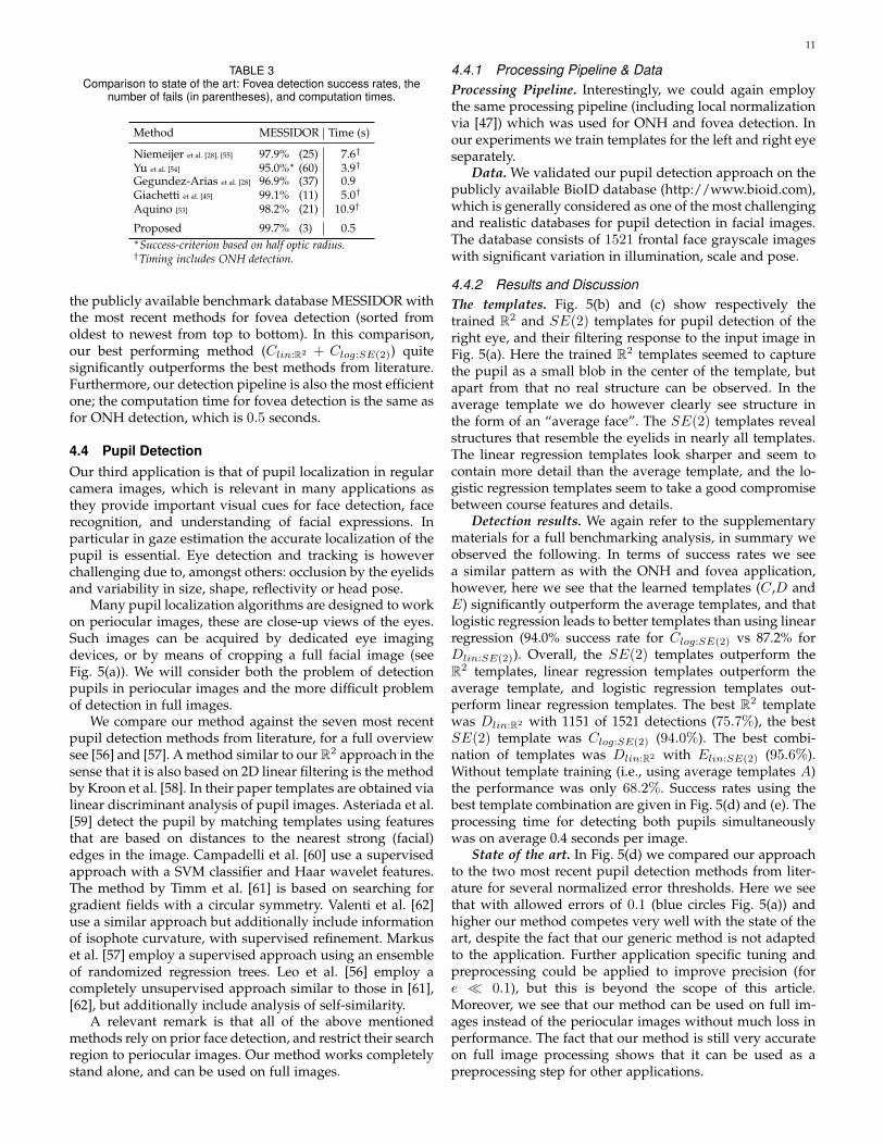
the publicly available benchmark database MESSIDOR withthe most recent methods for fovea detection (sorted fromoldest to newest from top to bottom). In this comparison,our best performing method (Clin:R2 + Clog:SE(2)) quitesignificantly outperforms the best methods from literature.Furthermore, our detection pipeline is also the most efficientone; the computation time for fovea detection is the same asfor ONH detection, which is 0.5 seconds.

4.4 Pupil DetectionOur third application is that of pupil localization in regularcamera images, which is relevant in many applications asthey provide important visual cues for face detection, facerecognition, and understanding of facial expressions. Inparticular in gaze estimation the accurate localization of thepupil is essential. Eye detection and tracking is howeverchallenging due to, amongst others: occlusion by the eyelidsand variability in size, shape, reflectivity or head pose.

Many pupil localization algorithms are designed to workon periocular images, these are close-up views of the eyes.Such images can be acquired by dedicated eye imagingdevices, or by means of cropping a full facial image (seeFig. 5(a)). We will consider both the problem of detectionpupils in periocular images and the more difficult problemof detection in full images.

We compare our method against the seven most recentpupil detection methods from literature, for a full overviewsee [56] and [57]. A method similar to our R2 approach in thesense that it is also based on 2D linear filtering is the methodby Kroon et al. [58]. In their paper templates are obtained vialinear discriminant analysis of pupil images. Asteriada et al.[59] detect the pupil by matching templates using featuresthat are based on distances to the nearest strong (facial)edges in the image. Campadelli et al. [60] use a supervisedapproach with a SVM classifier and Haar wavelet features.The method by Timm et al. [61] is based on searching forgradient fields with a circular symmetry. Valenti et al. [62]use a similar approach but additionally include informationof isophote curvature, with supervised refinement. Markuset al. [57] employ a supervised approach using an ensembleof randomized regression trees. Leo et al. [56] employ acompletely unsupervised approach similar to those in [61],[62], but additionally include analysis of self-similarity.

A relevant remark is that all of the above mentionedmethods rely on prior face detection, and restrict their searchregion to periocular images. Our method works completelystand alone, and can be used on full images.

4.4.1 Processing Pipeline & DataProcessing Pipeline. Interestingly, we could again employthe same processing pipeline (including local normalizationvia [47]) which was used for ONH and fovea detection. Inour experiments we train templates for the left and right eyeseparately.

Data. We validated our pupil detection approach on thepublicly available BioID database (http://www.bioid.com),which is generally considered as one of the most challengingand realistic databases for pupil detection in facial images.The database consists of 1521 frontal face grayscale imageswith significant variation in illumination, scale and pose.

4.4.2 Results and DiscussionThe templates. Fig. 5(b) and (c) show respectively thetrained R2 and SE(2) templates for pupil detection of theright eye, and their filtering response to the input image inFig. 5(a). Here the trained R2 templates seemed to capturethe pupil as a small blob in the center of the template, butapart from that no real structure can be observed. In theaverage template we do however clearly see structure inthe form of an “average face”. The SE(2) templates revealstructures that resemble the eyelids in nearly all templates.The linear regression templates look sharper and seem tocontain more detail than the average template, and the lo-gistic regression templates seem to take a good compromisebetween course features and details.

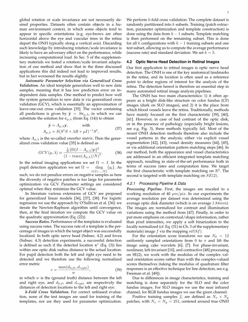
Detection results. We again refer to the supplementarymaterials for a full benchmarking analysis, in summary weobserved the following. In terms of success rates we seea similar pattern as with the ONH and fovea application,however, here we see that the learned templates (C ,D andE) significantly outperform the average templates, and thatlogistic regression leads to better templates than using linearregression (94.0% success rate for Clog:SE(2) vs 87.2% forDlin:SE(2)). Overall, the SE(2) templates outperform theR2 templates, linear regression templates outperform theaverage template, and logistic regression templates out-perform linear regression templates. The best R2 templatewas Dlin:R2 with 1151 of 1521 detections (75.7%), the bestSE(2) template was Clog:SE(2) (94.0%). The best combi-nation of templates was Dlin:R2 with Elin:SE(2) (95.6%).Without template training (i.e., using average templates A)the performance was only 68.2%. Success rates using thebest template combination are given in Fig. 5(d) and (e). Theprocessing time for detecting both pupils simultaneouslywas on average 0.4 seconds per image.

State of the art. In Fig. 5(d) we compared our approachto the two most recent pupil detection methods from liter-ature for several normalized error thresholds. Here we seethat with allowed errors of 0.1 (blue circles Fig. 5(a)) andhigher our method competes very well with the state of theart, despite the fact that our generic method is not adaptedto the application. Further application specific tuning andpreprocessing could be applied to improve precision (fore 0.1), but this is beyond the scope of this article.Moreover, we see that our method can be used on full im-ages instead of the periocular images without much loss inperformance. The fact that our method is still very accurateon full image processing shows that it can be used as apreprocessing step for other applications.

12

0.0%

10.0%

20.0%

30.0%

40.0%

50.0%

60.0%

70.0%

80.0%

90.0%

100.0%

0.025 0.05 0.075 0.1 0.125 0.15 0.175 0.2

Acc

ura

cy

Normalized error threshold

Markus 2014 - Perioc.

Leo 2014 - Perioc.

Proposed - Perioc.

Proposed - Full

Peri

ocu

lar

imag

eFu

ll im

age

Ref

eren

ce m

eth

od

s(p

erio

cula

r)

87

%

82

% 85

% 93

%

92

% 97

%

87

%

76

%

94

%

96

%

41

%

87

%

92

%

0%

10%

20%

30%

40%

50%

60%

70%

80%

90%

100%

Accuracy (normalized error ≤ 0.1)

Fig. 5. Overview of trained templates for right-eye pupil detection, and their responses to a challenging image from the BioID database. (a) Theexample input image with true pupil locations (blue circle with a radius that corresponds to a normalized error threshold of 0.1, see Eq. 39. Thewhite square indicates the periocular image region for the right eye. (b) The R2-type templates (top row) and their responses to the input image(bottom row). (c) The maximum intensity projections (over θ) of the SE(2)-type templates (top row) and their responses to the input image (bottomrow). Detected pupil locations are indicated with colored circles (green = correct, red = incorrect, based on a normalized error threshold of 0.1).(d) Accuracy curves generated by varying thresholds on the normalized error, in comparison with the two most recent methods from literature. (e)Accuracy (at a normalized error threshold of 0.1) comparison with pupil detection methods from literature.

If Fig. 5(e) we compared our approach to the sevenmost recent methods from literature (sorted from old tonew). Here we see that the only method outperforming ourmethod, at standard accuracy requirements (e ≤ 0.1), isthe method by Markus et al. [57]. Even when consideringprocessing of the full images the only other method thatoutperforms ours is the method by Timm et al. [61], whoseperformance is measured using periocular images.

4.5 General Observations

The application of our method to the three problems (ONH,fovea and pupil detection) showed the following:

1) State-of-the-art performance was achieved on threedifferent applications, using a single (generic) de-tection framework and without application specificparameter adaptations.

2) Cross correlation based template matching via datarepresentations on SE(2) improves results overstandard R2 filtering.

3) Trained templates, obtained using energy function-als of the form (1), often perform better than basic

average templates. In particular in pupil detectionthe optimization of templates proved to be essential.

4) Our newly introduced logistic regression approachleads to improved results in pupil detection viasingle templates. When combining templates weobserve only a small improvement of choosing lo-gistic regression (instead of linear regression) for theapplication of ONH and fovea detection.

5) Regularization in both linear and logistic regressionis important. Here both ridge and smoothing regu-larization priors have complementary benefits.

6) Our method does not rely on any other detectionsystems (such as ONH detection in the fovea appli-cation, or face detection in the pupil detection), andstill performs well compared to methods that do.

7) Our method is fast and parallelizable as it is basedon inner products, as such it could be efficientlyimplemented using convolutions.

5 CONCLUSION

In this paper we have presented an efficient cross-correlationbased template matching scheme for the detection of com-

13

bined orientation and blob patterns. Furthermore, we haveprovided a generalized regression framework for the con-struction of templates. The method relies on data repre-sentations in orientation scores, which are functions onthe Lie group SE(2), and we have provided the tools forproper smoothing priors via resolvent hypo-elliptic diffu-sion processes on SE(2) (solving time-integrated hypo-elliptic Brownian motions on SE(2)). The strength of themethod was demonstrated with two applications in reti-nal image analysis (the detection of the optic nerve head(ONH), and the detection of the fovea) and additionalexperiments for pupil detection in regular camera images.In the retinal applications we achieved state-of-the-art re-sults with an average detection rate of 99.83% on 1737images for ONH detection, and 99.32% on 1616 imagesfor fovea detection. Also on pupil detection we obtainedstate-of-the-art performance with a 95.86% success rate on1521 images. We showed that the success of the methodis due to the inclusion of both intensity and orientationfeatures in template matching. The method is also com-putationally efficient as it is entirely based on a sequenceof convolutions (which can be efficiently done using fastFourier transforms). These convolutions are parallelizable,which can further speed up our already fast experimen-tal Mathematica implementations that are publicly availableat http://erikbekkers.bitbucket.org/TMSE2.html. In futurework we plan to investigate the applicability of smoothingon SE(2) in variational settings, as this could also be usedin (sparse) line enhancement and segmentation problems.

ACKNOWLEDGMENTS

The authors would like to thank the groups that kindlymade available the benchmark datasets and annotations.The authors gratefully acknowledge Gonzalo Sanguinetti(TU/e) for fruitful discussions and feedback on thismanuscript. The research leading to the results of this articlehas received funding from the European Research Coun-cil under the European Community’s 7th Framework Pro-gramme (FP7/20072014)/ERC grant agreement No. 335555.This work is also part of the He Programme of InnovationCooperation, which is (partly) financed by the NetherlandsOrganisation for Scientific Research (NWO).

14

APPENDIX APROBABILISTIC INTERPRETATION OF THE SMOOTH-ING PRIOR IN SE(2)

In this section we relate the SE(2) smoothing prior totime resolvent hypo-elliptic2 diffusion processes on SE(2).First we aim to familiarize the reader with the concept ofresolvent diffusions on R2 in Subsec. A.1. Then we posein Subsec. A.2 a new problem (the single patch problem),which is a special case of our SE(2) linear regressionproblem, that we use to link the left-invariant regularizerto tue resolvents of hypo-elliptic diffusions on SE(2).

A.1 Resolvent Diffusion Processes

A classic approach to noise suppression in images is viadiffusion regularizations with PDE’s of the form [34]

∂∂τ u = ∆u,u|τ=0 = u0,

(40)

where ∆ denotes the Laplace operator. Solving (40) for anydiffusion time τ > 0 gives a smoothed version of the inputu0. The time-resolvent process of the PDE is defined by theLaplace transform with respect to τ ; time τ is integratedout using a memoryless negative exponential distributionP (T = τ) = αe−ατ . Then, the time integrated solutions

t(x) = α

∫ ∞0

u(x, τ)e−ατdτ,

with decay parameter α, are in fact the solutions

t = argmint∈L2(R2)

[‖t− t0‖2L2(R2) + λ

∫R2

‖∇t(x)‖2 dx

], (41)

with λ = α−1, and corresponding Euler-Lagrange equation

(I − λ∆)t = t0 ⇔ t = λ−1

(1

λ−∆

)−1

t0, (42)

to which we refer as the “resolvent” equation [63], as itinvolves operator (αI − ∆)−1, α = λ−1. In the next sub-sections, we follow a similar procedure with SE(2) insteadof R2, and show how the smoothing regularizer in Eq. (28)and (30) of the main article relates to Laplace transforms ofhypo-elliptic diffusions on the group SE(2) [9], [10].

A.2 The Fundamental Single Patch Problem

In order to grasp what the (anisotropic regularization term)in Eq. (28) and (30) of the main article actually means interms of stochastic interpretation/probabilistic line propa-gation, let us consider the following single patch problemand optimize

Esp(T ) = |(Gs ∗R2 T (·, ·, θ0)) (x0)− 1|2

+ λ

∫R2

∫ 2π

0‖∇T (x, θ)‖2Ddxdθ + µ‖T‖2L2(SE(2)), (43)

2. This diffusion process on SE(2) is called hypo-elliptic as its gen-erator equals (∂ξ)

2 + Dθθ(∂θ)2 and diffuses only in 2 directions in

a 3D space. This boils down to a sub-Riemannian manifold structure[9], [33]. Smoothing in the missing (∂η) direction is achieved via thecommutator: [∂θ, cos θ∂x + sin θ∂y ] = − sin θ∂x + cos θ∂y .

with (x0, θ0) = g0 := (x0, y0, θ0) ∈ SE(2) the fixed centerof the template, and with spatial Gaussian kernel

Gs(x) =1

4πse−‖x‖24s .

Regarding this problem, we note the following:

• In the original problem (28) of the main article wetake N = 1, with

Uf1(x, y, θ) = Gs(x− x0, y − y0) δθ0(θ) (44)

representing a local spatially smoothed spike inSE(2), and set y1 = 1. The general single patch case(for arbitrary Uf1 ) can be deduced by superpositionof such impulse responses.

• We use µ > 0 to suppress the output elsewhere.• We use 0 < s 1. This minimum scale due to

sampling removes the singularity at (0, 0) from thekernel that solves (43), as proven in [9].

Theorem 1. The solution to the single patch problem (43) coin-cides up to scalar multiplication with the time integrated hypo-elliptic Brownian motion kernel on SE(2) (depicted in Fig. 6).

Proof. We optimize Esp(T ) over the set S(SE(2)) of allfunctions T : SE(2) → R that are bounded and onSE(2), infinitely differentiable on SE(2)\g0, and rapidlydecreasing in spatial direction, and 2π periodic in θ. Weomit topological details on function spaces and Hormanderscondition [64]. Instead, we directly proceed with applyingthe Euler-Lagrange technique to the single patch problem:

∀δ∈S(SE(2)) : limε↓0

Esp(T + εδ)− Esp(T )

ε

= 0⇔

(S∗sSs + λR+ µI)T = S∗sy1 = S∗s1, (45)

with linear functional (distribution) Ss given by

(SsT ) = (Gs ∗R2 T (·, θ0))(x0),

and with regularization operator R given by

R = −∆SE(2) := −(Dθθ∂2θ +Dξξ∂

2ξ +Dηη∂

2η) ≥ 0.

Note that lims→0

Ss = δ(x0,θ0) in distributional sense, and thatthe constraint s > 0 is crucial for solutions T to be boundedat (x0, θ0). By definition the adjoint operator S∗s is given by

(S∗sy, T )L2(SE(2)) = (y, SsT ) = y∫R2 Gs(x− x0)T (x, θ0) dx

= y2π∫0

∫R2

Gs(x− x0)δθ0(θ)T (x, θ) dxdθ,

= (y Gs(· − x0)δθ0(·), T )L2(SE(2))

and thereby we deduce that

(S∗sy)(x, θ) = y Gs(x− x0)δθ0(θ),

S∗s (SsT ) = T s0 Gs(x− x0)δθ0(θ),

with ∞ > T s0 := (Gs ∗R2 T (·, θ0))(x0) > 1 for 0 < s 1.The Euler-Lagrange equation (45) becomes

(−λ∆SE(2) + µI)T = (1− T s0 )Gs(x− x0)δθ0(θ).

15

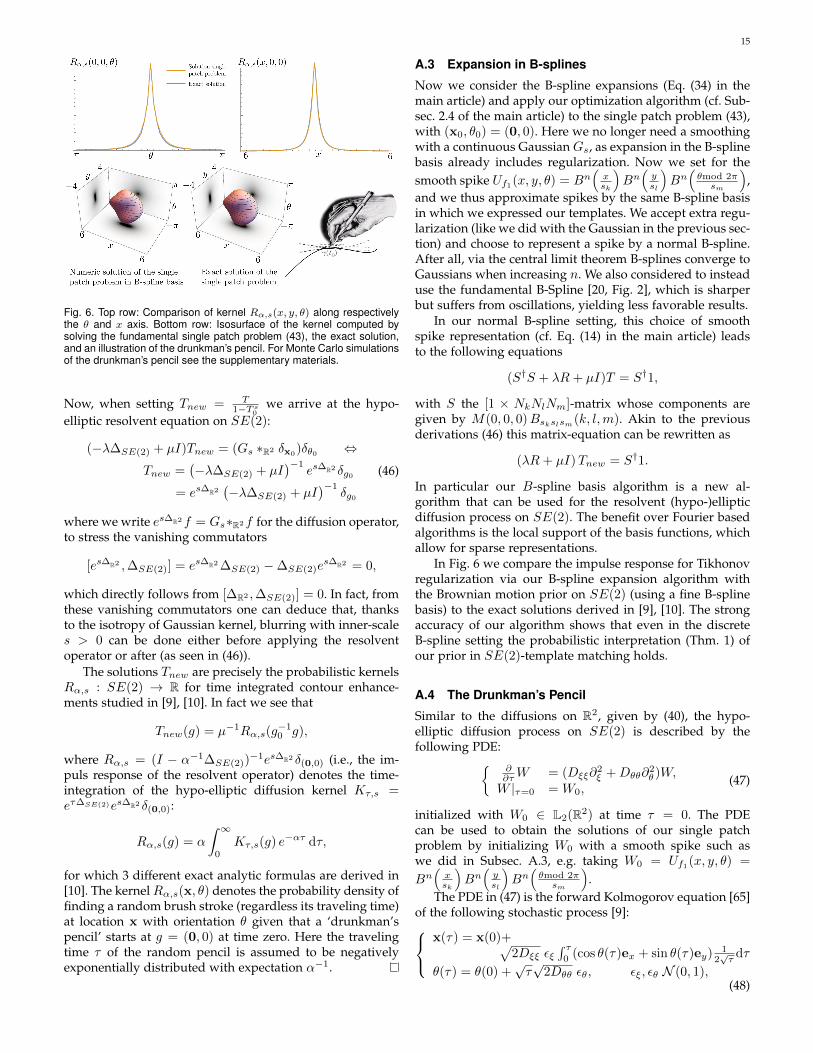
Fig. 6. Top row: Comparison of kernel Rα,s(x, y, θ) along respectivelythe θ and x axis. Bottom row: Isosurface of the kernel computed bysolving the fundamental single patch problem (43), the exact solution,and an illustration of the drunkman’s pencil. For Monte Carlo simulationsof the drunkman’s pencil see the supplementary materials.

Now, when setting Tnew = T1−T s

0we arrive at the hypo-

elliptic resolvent equation on SE(2):

(−λ∆SE(2) + µI)Tnew = (Gs ∗R2 δx0)δθ0 ⇔

Tnew =(−λ∆SE(2) + µI

)−1es∆R2 δg0

= es∆R2(−λ∆SE(2) + µI

)−1δg0

(46)

where we write es∆R2 f = Gs∗R2f for the diffusion operator,to stress the vanishing commutators

[es∆R2 ,∆SE(2)] = es∆R2 ∆SE(2) −∆SE(2)es∆R2 = 0,

which directly follows from [∆R2 ,∆SE(2)] = 0. In fact, fromthese vanishing commutators one can deduce that, thanksto the isotropy of Gaussian kernel, blurring with inner-scales > 0 can be done either before applying the resolventoperator or after (as seen in (46)).

The solutions Tnew are precisely the probabilistic kernelsRα,s : SE(2) → R for time integrated contour enhance-ments studied in [9], [10]. In fact we see that

Tnew(g) = µ−1Rα,s(g−10 g),

where Rα,s = (I − α−1∆SE(2))−1es∆R2 δ(0,0) (i.e., the im-

puls response of the resolvent operator) denotes the time-integration of the hypo-elliptic diffusion kernel Kτ,s =eτ∆SE(2)es∆R2 δ(0,0):

Rα,s(g) = α

∫ ∞0

Kτ,s(g) e−ατ dτ,

for which 3 different exact analytic formulas are derived in[10]. The kernelRα,s(x, θ) denotes the probability density offinding a random brush stroke (regardless its traveling time)at location x with orientation θ given that a ‘drunkman’spencil’ starts at g = (0, 0) at time zero. Here the travelingtime τ of the random pencil is assumed to be negativelyexponentially distributed with expectation α−1.

A.3 Expansion in B-splines

Now we consider the B-spline expansions (Eq. (34) in themain article) and apply our optimization algorithm (cf. Sub-sec. 2.4 of the main article) to the single patch problem (43),with (x0, θ0) = (0, 0). Here we no longer need a smoothingwith a continuous Gaussian Gs, as expansion in the B-splinebasis already includes regularization. Now we set for thesmooth spike Uf1(x, y, θ) = Bn

(xsk

)Bn(ysl

)Bn(θmod 2πsm

),

and we thus approximate spikes by the same B-spline basisin which we expressed our templates. We accept extra regu-larization (like we did with the Gaussian in the previous sec-tion) and choose to represent a spike by a normal B-spline.After all, via the central limit theorem B-splines converge toGaussians when increasing n. We also considered to insteaduse the fundamental B-Spline [20, Fig. 2], which is sharperbut suffers from oscillations, yielding less favorable results.

In our normal B-spline setting, this choice of smoothspike representation (cf. Eq. (14) in the main article) leadsto the following equations

(S†S + λR+ µI)T = S†1,

with S the [1 × NkNlNm]-matrix whose components aregiven by M(0, 0, 0)Bskslsm(k, l,m). Akin to the previousderivations (46) this matrix-equation can be rewritten as

(λR+ µI)Tnew = S†1.

In particular our B-spline basis algorithm is a new al-gorithm that can be used for the resolvent (hypo-)ellipticdiffusion process on SE(2). The benefit over Fourier basedalgorithms is the local support of the basis functions, whichallow for sparse representations.

In Fig. 6 we compare the impulse response for Tikhonovregularization via our B-spline expansion algorithm withthe Brownian motion prior on SE(2) (using a fine B-splinebasis) to the exact solutions derived in [9], [10]. The strongaccuracy of our algorithm shows that even in the discreteB-spline setting the probabilistic interpretation (Thm. 1) ofour prior in SE(2)-template matching holds.

A.4 The Drunkman’s Pencil

Similar to the diffusions on R2, given by (40), the hypo-elliptic diffusion process on SE(2) is described by thefollowing PDE:

∂∂τW = (Dξξ∂

2ξ +Dθθ∂

2θ )W,

W |τ=0 = W0,(47)

initialized with W0 ∈ L2(R2) at time τ = 0. The PDEcan be used to obtain the solutions of our single patchproblem by initializing W0 with a smooth spike such aswe did in Subsec. A.3, e.g. taking W0 = Uf1(x, y, θ) =

Bn(xsk

)Bn(ysl

)Bn(θmod 2πsm

).

The PDE in (47) is the forward Kolmogorov equation [65]of the following stochastic process [9]:

x(τ) = x(0)+√2Dξξ εξ

∫ τ0 (cos θ(τ)ex + sin θ(τ)ey) 1

2√τ

dτ

θ(τ) = θ(0) +√τ√

2Dθθ εθ, εξ, εθ N (0, 1),(48)

16

Fig. 7. Stochastic random process for contour enhancement.

where εξ and εθ are sampled from a normal distribu-tion with expectation 0 and unit standard deviation. Thestochastic process in (48) can be interpreted as the motionof a drunkman’s pencil: it randomly moves forward andbackwards, and randomly changes its orientation along theway. The resolvent hypo-elliptic diffusion kernels Rα,s(g)(solutions to the fundamental single patch problem, up toscalar multiplication) can then also be obtained via MonteCarlo simulations, where the stochastic process is sampledmany times with a negatively exponentially distributedtraveling time (P (T = τ) = αe−ατ ) in order to be able toestimate the probability density kernel Rα,s(g). This processis illustrated in Fig. 7.

APPENDIX BTHE SMOOTHING REGULARIZATION MATRIX RWhen expanding the templates t and T in a finite B-Splinebasis (Sec. 2 and 3 of the main article), the energy functionals(7), (11), (28) and (30) of the main article can be expressedin matrix vector form. The following theorems summarizehow to compute the matrixR, which encodes the smoothingprior, for respectively the R2 and SE(2) case.

Lemma 1. The discrete smoothing regularization-term of energyfunctional (7) of the main article can be expressed directly in theB-Spline coefficients c as follows∫∫

R2

‖∇t(x, y)‖2dxdy = c†Rc, (49)

with c given by Eq. (16) of the main article, and with

R = Rkx ⊗Rlx +Rky ⊗Rly, (50)

a [NkNl × NkNl] matrix. The elements of the matrices in (50)are given by

Rkx(k, k′) = − 1sk∂2B2n+1

∂x2 (k′ − k)

Rlx(l, l′) = slB2n+1(l′ − l),

Rky(k, k′) = skB2n+1(k′ − k),

Rly(l, l′) = − 1sl∂2B2n+1

∂y2 (l′ − l).

(51)

Proof. For the sake of readability we divide theregularization-term in two parts:∫∫

R2‖∇t(x, y)‖2dxdy =∫∫

R2

∣∣ ∂t∂x (x, y)

∣∣2+∣∣∣ ∂t∂y (x, y)

∣∣∣2 dxdy,

(52)where

Rx =∫∫

R2

∣∣ ∂t∂x (x, y)

∣∣2 dxdy, and

Ry =∫∫

R2

∣∣∣ ∂t∂y (x, y)∣∣∣2 dxdy.

We first derive the matrix-vector representation of Rx asfollows:

Rx =∫∫

R2

∣∣ ∂t∂x (x, y)

∣∣2 dxdy

=Nk∑

k,k′=1

Nl∑l,l′=1

∫∫R2 ck,l

∂Bn

∂x ( xsk − k)Bn( ysl − l)

ck,l∂Bn

∂x ( xsk − k′)Bn( ysl − l

′)dxdy

=Nk∑

k,k′=1

Nl∑l,l′=1

ck,lck′,l′[∞∫−∞

∂Bn

∂x ( xsk − k)∂Bn

∂x ( xsk − k′)dx

][∞∫−∞

Bn( ysl − l)Bn( ysl − l

′)dy

]1=

Nk∑k,k′=1

Nl∑l,l′=1

ck,lck′,l′[

1sk

(∂Bn

∂x ∗∂Bn

∂x

)(k′ − k)

][sl (B

n ∗Bn) (l′ − l)]2=

M∑k,k′=1

N∑l,l′=1

ck,lck′,l′[

1sk∂2B2n+1

∂x2 (k′ − k)]

[slB

2n+1(l′ − l)]

= c†(Rkx ⊗Rlx)c.(53)

Here the following properties are used:

1) The integrals of shifted B-splines can be expressedas convolutions:∫ ∞

−∞

∂Bn

∂x

(x

sk− k

)∂Bn

∂x

(x

sk− k′

)dx

= − 1

sk

∫ ∞−∞

∂Bn

∂u(u)

∂Bn

∂u((k′ − k)− u)du

= − 1

sk

(∂Bn

∂u∗ ∂B

n

∂u

)(k′ − k).

This is easily verified by substitution of integrationvariable (u = − x

sk+ k) and noting that Bn(x) =

Bn(−x) and ∂Bn

∂x (x) = −∂Bn

∂x (−x).2) Convolution of two B-splines Bn of order n results

in a B-Spline B2n+1 of order 2n+ 1:

Bn ∗Bn = B2n+1.

The elements of the matrices Rky and Rly are derived in asimilar manner.

As a result of Lemma 1 we can state the following.

Corollary 1. Let V = spanBnk,l, with k = 1, . . . , Nk, l =1, . . . , Nl, and shifted B-splines Bnk,l of order n (cf. Subsec. 2.4 ofthe main article). Let the energy function EBlin : RNkNl → R+ begiven by Eq. (13) of the main article. Then the optimal continuoustemplate of the constrained optimization problem (cf. Eq. (7) of themain article)

t∗ = argmint∈V

Elin(t)

has coefficients c∗ w.r.t. the B-spline basis for V , that are theunique solution of

∇cEB(c∗) = 0,

which boils down to Eq. (14) of the main article.

17

Lemma 2. The discrete regularization-term of energy functional(28) of the main article can be expressed directly in the B-Splinecoefficients:∫∫∫

SE(2)‖∇T‖D dxdydθ = cT (DξξRξ+DηηRη+DθθRθ)c.

(54)Matrix Rξ is given by

Rξ =(RIxξ ⊗R

Iyξ ⊗R

Iθξ

)+(RIIxξ ⊗RIIyξ ⊗RIIθξ

)+(RIIIxξ ⊗RIIIyξ ⊗RIIIθξ

)+(RIV xξ ⊗RIV yξ ⊗RIV θξ

)(55)

with the elements of the matrices used in the Kronecker productsgiven by

RIxξ (k, k′) = − 1sk∂2B2n+1

∂x2 (k′ − k),

RIyξ (l, l′) = slB2n+1(l′ − l),

RIθξ (m,m′) =π∫0

cos2(θ)Bn( θsm−m)Bn( θ

sm−m′)dθ,

(56)RIIxξ (k, k′) = −RIIIxξ (k, k′) = ∂B2n+1

∂x (k′ − k),

RIIyξ (l, l′) = −RIIIyξ (l, l′) = −∂B2n+1

∂y (l′ − l),RIIθξ (m,m′) = RIIIθξ (m,m′) =

π∫0

cos(θ) sin(θ)Bn( θsm−m)Bn( θ

sm−m′)dθ,

(57)RIV xξ (k, k′) = skB

2n+1(k′ − k),

RIV yξ (l, l′) = − 1sl∂2B2n+1

∂y2 (l′ − l),

RIV θξ (m,m′) =π∫0

sin2(θ)Bn( θsm−m)Bn( θ

sm−m′)dθ.

(58)Matrix Rη is given by

Rη =(RIIxξ ⊗RIIyξ ⊗RIV θξ

)−(RIIxξ ⊗RIIyξ ⊗RIIθξ

)−(RIIIxξ ⊗RIIIyξ ⊗RIIIθξ

)+(RIV xξ ⊗RIV yξ ⊗RIθξ

).

(59)

Matrix Rθ is given by

Rθ =(Rxθ ⊗R

yθ ⊗R

θθ

), (60)

with the elements of the matrices given by

Rxθ (k, k′) = skB2n+1(k′ − k),

Ryθ(l, l′) = slB2n+1(l′ − l),

Rθθ(m,m′) = − 1

sm∂2B2n+1

∂θ2 (m′ −m).(61)

Proof. The proof of Lemma 2 follows the same steps as in theproof of Lemma 1, only here left-invariant derivatives areused (cf. Eq. (24) of the main article). The four separate termsI − IV of Eq. (55) arise from the left invariant derivative ∂ξ :∣∣∣∂T∂ξ ∣∣∣2 =

∣∣∣cos(θ)∂T∂x + sin(θ)∂T∂y

∣∣∣2.

Lemma 2 has the following consequence.

Corollary 2. Let V = spanBnk,l,m, with k = 1, . . . , Nk, l =1, . . . , Nl,m = 1, . . . , Nm, and shifted B-splines Bnk,l,m of ordern (cf. Subsec. 3.5 of the main article). Let the energy functionEBlin : RNkNlNm → R+ be given by

EBlin(c) =1

N‖Sc− y‖2 + c†(λR+ µI)c

With S and y given by (33) of the main article and with R =DξξRξ +DηηRη +DθθRθ given in Lemma 2. Then the optimalcontinuous template of the constrained optimization problem (cf.Eq. (28) of the main article)

T ∗ = argminT∈V

Elin(T )

has coefficients c∗ w.r.t. the B-spline basis for V that are theunique solution of

∇cEB(c∗) = 0.

This boils down to Eq. (14) of the main article, but then onRNkNlNm with matrices R and S given above.

APPENDIX CNORMALIZED CROSS CORRELATION

In most applications it is necessary to make the detectionsystem invariant to local contrast and luminosity changes.In our template matching framework this can either beachieved via certain pre-processing steps that filter out thesevariations, or by means of normalized cross-correlation. Innormalized cross-correlation, both the template as well asthe image are (locally) normalized to zero mean and unitstandard deviation (with respect to the inner product usedin the cross-correlations). In this section, we explain the nec-essary adaptations to extend the standard cross-correlationbased framework to normalized cross-correlations.

C.1 Normalized Cross-Correlation in R2

In the usual cross-correlation based template matching ap-proach, as described in Sec. 2 of the main article, we relyon the standard L2(R2) inner product (Eq. (6) of the mainarticle). In normalized cross-correlation it is however conve-nient to extend this inner product to include a windowingfunction m which indicates the relevant region (support)of the template. As such, the inner product with respect towindowing function m is given by

(t, f)L2(R2,mdx) :=

∫R2

t(x)f(x)m(x)dx, (62)

with associated norm ‖·‖L2(R2,mdx) =√

(·, ·)L2(R2,mdx). Thewindowing function has to be a smooth function m : R2 →R+ with

∫R2 m(x)dx = 1. In this work, the use of a window

m is also convenient to deal with boundary conditions in theoptimization problems for template construction. We define

m(x) := ς e−‖x‖2

s

n∑i=0

(‖x‖2/s)i

i!, (63)

which smoothly approximates the indicator function1[0,r](‖x‖), covering a disk with radius r, when settings = 2r2

1+2n , see e.g. [7, Fig. 2]. The constant ς normalizesthe function such that

∫R2 m(x)dx = 1.

In normalized cross-correlation the image is locally nor-malized (at position x) to zero mean and unit standarddeviation, which is done as follows

fx(x) :=f(x)− 〈f〉Txm

‖f(x)− 〈f〉Txm‖L2(R2,Txmdx), (64)

18

with local mean 〈f〉m = (1, f)L2(R2,mdx). Template t can beobtained via normalization of a given template t via

t(x) :=t(x)− 〈t〉m

‖t(x)− 〈t〉m‖L2(R2,mdx). (65)

Template matching is then done in the usual way (via(4) of the main article), however now t and fx are usedinstead of t and f . In fact, the entire R2 cross-correlationtemplate matching, and template optimization frameworkis extended to normalized cross-correlation by substitutingall instances of t with t, f with fx, and (·, ·)L2(R2) with(·, ·)L2(R2,mdx) in Sec. 2 of the main article. However, sincetemplates t are directly constructed via the minimizationof energy functionals, we will not explictely normalizethe templates, unless they are obtained by other methods.E.g., Eq. (65) is used in the main article to construct basictemplates obtained by averaging positive object patches(Subsec. 4.1 of the main article).

C.2 Normalized Cross-Correlation in SE(2)

Similar to the R2 case, templates and orientation scores arelocally normalized to zero mean and unit standard devi-ation, however, now with respect to the L2(SE(2),Mdg)inner product, which is given by

(T,Uf )L2(SE(2),Mdg) :=∫R2

∫ 2π

0T (x, θ)Uf (x, θ)M(x, θ)dxdθ, (66)

with norm ‖·‖L2(SE(2),Mdg) =√

(·, ·)L2(SE(2),Mdg). Alsohere windowing function M indicates the support of thetemplate, and has the property

∫R2

∫ 2π0 M(x, θ)dxdθ = 1.

We defineM(x, θ) :=

1

2πm(x), (67)

independent of θ and with m(x) given by (63).The (locally at g) normalized orientation score and tem-

plate T are then given by

Uf,g(x, θ) :=Uf (x, θ)− 〈Uf 〉LgM

‖Uf (x, θ)− 〈Uf 〉LgM‖L2(SE(2),LgMdg)

, (68)

T (x, θ) :=T (x, θ)− 〈T 〉M

‖T (x, θ)− 〈T 〉M‖L2(SE(2),Mdg)

, (69)

with mean 〈Uf 〉M = (1, Uf )L2(SE(2),Mdg)).

C.3 Efficient local normalization of fx and Uf,g.

Since the normalized image fx depends on the location x itneeds to be calculated for every translation of the template,which makes normalized cross-correlation computationallyexpensive. Therefore, (64) can be approximated by assumingthat the local average is approximately constant in the areacovered by m. That is, assuming 〈f〉Txm(x) ≈ 〈f〉Txm(x) =(m?f)(x) for ‖x− x‖ < r, with r the radius that determinesthe extent of m, (64) is approximated as follows:

fx(x) ≈f(x)− (m ? f)(x)√

(m ? (f − (m ? f))2)(x). (70)

Similarly, in the SE(2)-case (68) can be approximated via

Uf,g(x, θ) ≈Uf (x, θ)− (M ?SE(2) Uf )(x, θ)√

(M ?SE(2) (Uf − (M ?SE(2) Uf ))2)(x, θ).

(71)

C.4 Including a Region of Interest Mask

Depending on the application, large portions of the imagemight be masked out. This for example the case in retinalimages (see circular masks in Fig. 9). To deal with this,template matching is only performed inside the region ofinterest defined by a mask image mroi : R2 → 0, 1.Including such a mask is important in normalized templatematching, and can be done by replacing the standard innerproducts by

(t, f)roiL2(R2,m,dx) :=(t, fmroi)L2(R2,m,dx)

(1,mroi)L2(R2,m,dx), (72)

(T,Uf )roiL2(SE(2),M,dg) :=(T,UfM

roi)L2(SE(2),M,dg)

(1,Mroi)L2(SE(2),M,dg), (73)

with Mroi(x, θ) = mroi(x).

APPENDIX DADDITIONAL DETAILS ON THE DETECTION PROB-LEMS

In this section we describe additional details about theimplementation and results of the three detection problemsdiscussed in the main article.

D.1 Training Samples

In all three applications training samples were used to com-pute the templates. Positive training samples were centeredaround the object of interest. Negative training sampleswere centered around random locations in the image, butnot within a certain distances to the true positive objectlocation. In the retinal applications this distance was oneoptic disk radius, in the pupil detection application this wasa normalized distance of 0.1 (cf. Eq.(39) of the main article).An selection of the 2D image pathes that were used in theexperiments are shown in Fig. 8.

D.2 Processing Pipeline, Settings and Timings

D.2.1 Processing PipelineIn all three application the same processing pipeline wasused. The pipeline can be divided into the following 5 steps:

1) Resizing. Each input image is resized to a certainoperating resolution and cropped to remove largeregions with value 0 (outside the field of view maskin retinal images, see e.g. Fig. 9). The retinal imagesare resized such that the pixel size was approxi-mately 40µm/pix. In the pupil detection applicationno rescaling or cropping was done.

2) R2-Processing. In all three applications we applied alocal intensity and contrast normalization step usingan adaptation of [47] which we explain below. The

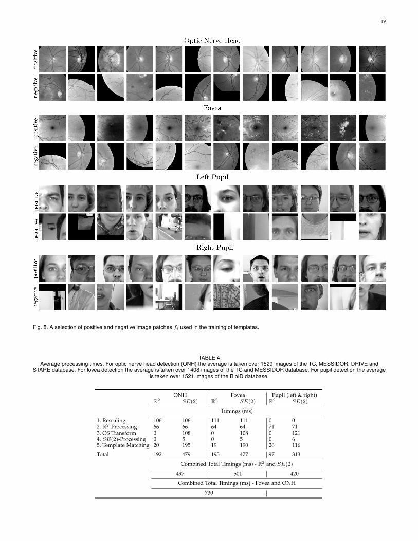
19

Fig. 8. A selection of positive and negative image patches fi used in the training of templates.

TABLE 4Average processing times. For optic nerve head detection (ONH) the average is taken over 1529 images of the TC, MESSIDOR, DRIVE and

STARE database. For fovea detection the average is taken over 1408 images of the TC and MESSIDOR database. For pupil detection the averageis taken over 1521 images of the BioID database.

ONH Fovea Pupil (left & right)R2 SE(2) R2 SE(2) R2 SE(2)

Timings (ms)

1. Rescaling 106 106 111 111 0 02. R2-Processing 66 66 64 64 71 713. OS Transform 0 108 0 108 0 1214. SE(2)-Processing 0 5 0 5 0 65. Template Matching 20 195 19 190 26 116

Total 192 479 195 477 97 313

Combined Total Timings (ms) - R2 and SE(2)

497 501 420

Combined Total Timings (ms) - Fovea and ONH

730

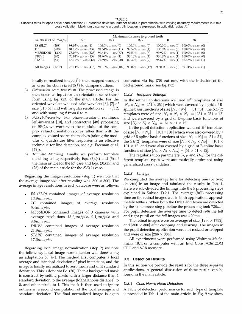
20

TABLE 5Success rates for optic nerve head detection (± standard deviation, number of fails in parenthesis) with varying accuracy requirements in 5-fold

cross validation. Maximum distance to ground truth location is expressed in optic disk radius R.

Maximum distance to ground truthDatabase (# of images) R/8 R/4 R/2 R 2R

ES (SLO) (208) 98.05% ± 2.04% (4) 100.0% ± 0.00% (0) 100.0% ± 0.00% (0) 100.0% ± 0.00% (0) 100.0% ± 0.00% (0)TC (208) 84.19% ± 4.34% (33) 94.54% ± 3.51% (11) 99.52% ± 1.06% (1) 100.0% ± 0.00% (0) 100.0% ± 0.00% (0)MESSIDOR (1200) 73.07% ± 3.69% (323) 94.41% ± 1.47% (67) 99.50% ± 0.46% (6) 99.92% ± 0.19% (1) 100.0% ± 0.00% (0)DRIVE (40) 70.84% ± 26.0% (13) 91.69% ± 12.3% (4) 98.18% ± 4.07% (1) 98.18% ± 4.07% (1) 100.0% ± 0.00% (0)STARE (81) 48.12% ± 10.27% (42) 74.94% ± 6.52% (20) 89.39% ± 8.16% (9) 98.67% ± 2.98% (1) 98.67% ± 2.98% (1)

All Images (1737) 76.11% ± 2.58% (415) 94.13% ± 0.79% (102) 99.02% ± 0.26% (17) 99.83% ± 0.26% (3) 99.94% ± 0.13% (1)

locally normalized image f is then mapped throughan error function via erf(8f) to dampen outliers.

3) Orientation score transform. The processed image isthen taken as input for an orientation score trans-form using Eq. (23) of the main article. For theoriented wavelets we used cake wavelets [6], [7] ofsize [51×51] and with angular resolution sθ = π/12,and with sampling θ from 0 to π.

4) SE(2)-Processing. For phase-invariant, nonlinear,left-invariant [10], and contractive [48] processingon SE(2), we work with the modulus of the com-plex valued orientation scores rather than with thecomplex-valued scores themselves (taking the mod-ulus of quadrature filter responses is an effectivetechnique for line detection, see e.g. Freeman et al.[49]).

5) Template Matching. Finally we perform templatematching using respectively Eqs. (3),(4) and (5) ofthe main article for the R2 case and Eqs. (3),(25) and(26) of the main article for the SE(2) case.

Regarding the image resolutions (step 1) we note thatthe average image size after rescaling was [300 × 300]. Theaverage image resolutions in each database were as follows:

• ES (SLO) contained images of average resolution13.9µm/pix.

• TC contained images of average resolution9.4µm/pix.

• MESSIDOR contained images of 3 cameras withaverage resolutions 13.6µm/pix, 9.1µm/pix and8.6µm/pix.

• DRIVE contained images of average resolution21.9µm/pix.

• STARE contained images of average resolution17.6µm/pix.

Regarding local image normalization (step 2) we notethe following. Local image normalization was done usingan adaptation of [47]. The method first computes a localaverage and standard deviation of pixel intensities, and theimage is locally normalized to zero mean and unit standarddeviation. This is done via Eq. (70). Then a background maskis construct by setting pixels with a larger distance than 1standard deviation to the average (Mahalanobis distance) to0, and other pixels to 1. This mask is then used to ignoreoutliers in a second computation of the local average andstandard deviation. The final normalized image is again

computed via Eq. (70) but now with the inclusion of thebackground mask, see Eq. (72).

D.2.2 Template SettingsIn the retinal applications we used R2 templates of size[Nx×Ny] = [251× 251] which were covered by a grid of B-spline basis functions of size [Nk×Nl] = [51×51], the SE(2)templates were of size [Nx × Ny × Nθ] = [251 × 251 × 12]and were covered by a grid of B-spline basis functions ofsize [Nk ×Nl ×Nm] = [51× 51× 12].

In the pupil detection application we used R2 templatesof size [Nx×Ny] = [101×101] which were also covered by agrid of B-spline basis functions of size [Nk×Nl] = [51×51],the SE(2) templates were of size [Nx ×Ny ×Nθ] = [101×101 × 12] and were also covered by a grid of B-spline basisfunctions of size [Nk ×Nl ×Nm] = [51× 51× 12].

The regularization parameters (λ, µ and Dθθ) for the dif-ferent template types were automatically optimized usinggeneralized cross validation.

D.2.3 TimingsWe computed the average time for detecting one (or two)object(s) in an image and tabulated the results in Tab. 4.Here we sub-divided the timings into the 5 processing stepsexplained in Subsec. D.2.1. The average (full) processingtime on the retinal images was in both applications approxi-mately 500ms. When both the ONH and fovea are detectedby the same processing pipeline the processing took 730ms.For pupil detection the average time to detect both the leftand right pupil on the full images was 420ms.

The retinal images were on average of size [1230×1792],and [300 × 300] after cropping and resizing. The images inthe pupil detection application were not resized or croppedand were of size [286× 384].

All experiments were performed using Wolfram Mathe-matica 10.4, on a computer with an Intel Core i703612QMCPU and 8GB memory.

D.3 Detection Results

In this section we provide the results for the three separateapplications. A general discussion of these results can befound in the main article.

D.3.1 Optic Nerve Head DetectionA Table of detection performance for each type of templateis provided in Tab. 1 of the main article. In Fig. 9 we show

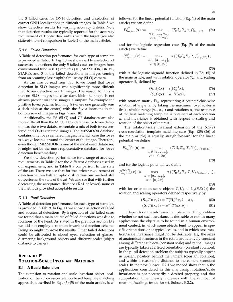
21

the 3 failed cases for ONH detection, and a selection ofcorrect ONH localizations in difficult images. In Table 5 weshow detection results for varying accuracy criteria. Notethat detection results are typically reported for the accuracyrequirement of 1 optic disk radius with the target (see alsostate-of-the-art comparison in Table 2 of the main article).

D.3.2 Fovea Detection

A Table of detection performance for each type of templateis provided in Tab. 6. In Fig. 10 we show next to a selection ofsuccessful detections the only 5 failed cases on images fromconventional fundus (CF) cameras (TC, MESSIDOR, DRIVE,STARE), and 3 of the failed detections in images comingfrom an scanning laser ophthalmoscopy (SLO) camera.

As can also be read from Tab. 6, we found that foveadetection in SLO images was significantly more difficultthan fovea detection in CF images. The reason for this isthat on SLO images the clear dark blob-like shape is notalways present on these images. Compare for example thepositive fovea patches from Fig. 8 (where one generally seesa dark blob at the center) with the fovea locations in thebottom row of images in Figs. 9 and 10.

Additionally, the ES (SLO) and CF databases are alsomore difficult than the MESSIDOR database for fovea detec-tion, as these two databases contain a mix of both fovea cen-tered and ONH centered images. The MESSIDOR databasecontains only fovea centered images, in which case the foveais always located around the center of the image. Therefore,even though MESSIDOR is one of the most used databases,it might not be the most representative database for foveadetection benchmarking.

We show detection performance for a range of accuracyrequirements in Table 7 for the different databases used inour experiments, and in Table 8 a comparison to the stateof the art. There we see that for the stricter requirement ofdetection within half an optic disk radius our method stilloutperforms the state of the art. We also see that with furtherdecreasing the acceptance distance (R/4 or lower) none ofthe methods provided acceptable results.

D.3.3 Pupil Detection

A Table of detection performance for each type of templateis provided in Tab. 9. In Fig. 11 we show a selection of failedand successful detections. By inspection of the failed caseswe found that a main source of failed detections was due torotations of the head. As stated in the previous section D.2we did not employ a rotation invariant detection scheme.Doing so might improve the results. Other failed detectionscould be attributed to closed eyes, reflection of glasses,distracting background objects and different scales (objectdistance to camera).

APPENDIX EROTATION-SCALE INVARIANT MATCHING

E.1 A Basic Extension

The extension to rotation and scale invariant object local-ization of the 2D cross-correlation based template matchingapproach, described in Eqs. (3)-(5) of the main article, is as

follows. For the linear potential function (Eq. (4) of the mainarticle) we can define

PR2

lin,inv(x) := maxa ∈ [a−, a+],α ∈ [0, 2π)

(TxSaRα t, f)L2(R2), (74)

and for the logistic regression case (Eq. (5) of the mainarticle) we define

PR2

log,inv(x) := maxa ∈ [a−, a+],α ∈ [0, 2π)

σ((TxSaRα t, f)L2(R2)

),

(75)with σ the logistic sigmoid function defined in Eq. (5) ofthe main article, and with rotation operator Rα and scalingoperator Sa defined by

(Rαt)(x) = t(R−1α x), (76)

(Sat)(x) = a−1t(ax), (77)

with rotation matrix Rα representing a counter clockwiserotation of angle α. By taking the maximum over scales a(in a suitable range [a−, a+]) and rotations α, the responseof the best matching template is obtained at each locationx, and invariance is obtained with respect to scaling androtation of the object of interest.

The rotation/scale invariant extension of the SE(2)cross-correlation template matching case (Eqs. (25)-(26) ofthe main article) is equally straightforward; for the linearpotential we define

PSE(2)lin,inv(x) := max

a ∈ [a−, a+],α ∈ [0, 2π)

(TxSaRα T,Uf )L2(SE(2)),

(78)and for the logistic potential we define

PSE(2)log,inv(x) := max

a ∈ [a−, a+],α ∈ [0, 2π)

σ((TxSaRα T,Uf )L2(SE(2))

),

(79)with for orientation score objects T,Uf ∈ L2(SE(2)) therotation and scaling operators defined respectively by

(RαT )(x, θ) = T (R−1α x, θ − α), (80)

(SaT )(x, θ) = a−1T (ax, θ). (81)

It depends on the addressed template matching problemwhether or not such invariance is desirable or not. In manyapplications the object is to be found in a human environ-ment context, in which some objects tend to appear in spe-cific orientations or at typical scales, and in which case rota-tion/scale invariance might not be desirable. E.g. the sizesof anatomical structures in the retina are relatively constantamong different subjects (constant scale) and retinal imagesare typically taken at a fixed orientation (constant rotation).In the pupil detection problem the subjects typically appearin upright position behind the camera (constant rotation),and within a reasonable distance to the camera (constantscale). In the next Subsec. E.2.1 we indeed show that in theapplications considered in this manuscript rotation/scaleinvariance is not necessarily a desired property, and thatcomputation time linearly increases with the number ofrotations/scalings tested for (cf. Subsec. E.2.2).

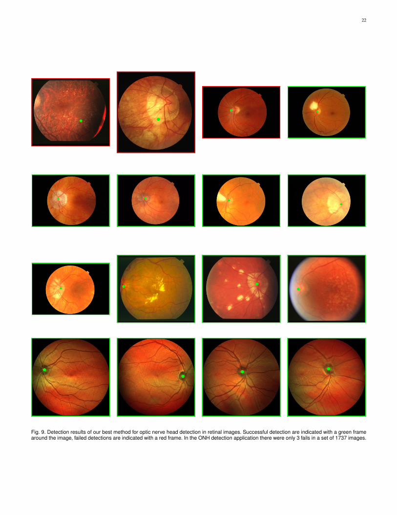
22

Fig. 9. Detection results of our best method for optic nerve head detection in retinal images. Successful detection are indicated with a green framearound the image, failed detections are indicated with a red frame. In the ONH detection application there were only 3 fails in a set of 1737 images.

23

TABLE 6Average template matching results (± standard deviation) for fovea detection in 5-fold cross validation, number of failed detections in parentheses.

Template ES (SLO) TC MESSIDOR All ImagesID 208 208 1200 1616

R2 templates

AR2 76.36% ± 6.79% (49) 98.24% ± 2.74% (3) 98.41% ± 0.22% (19) 95.60% ± 0.98% (71)

Blin:R2 23.50% ± 3.81% (159) 31.66% ± 9.03% (142) 51.19% ± 5.97% (587) 45.07% ± 3.33% (888)Clin:R2 45.65% ± 8.61% (113) 98.24% ± 2.74% (3) 98.59% ± 0.36% (17) 91.77% ± 1.26% (133)Dlin:R2 44.21% ± 4.62% (116) 99.49% ± 1.14% (1) 98.84% ± 0.31% (14) 91.90% ± 0.59% (131)Elin:R2 46.10% ± 8.11% (112) 98.86% ± 1.57% (2) 98.67% ± 0.34% (16) 91.95% ± 1.18% (130)

Blog:R2 1.43% ± 1.31% (205) 10.27% ± 5.09% (185) 20.07% ± 3.00% (959) 16.53% ± 2.52% (1349)Clog:R2 9.59% ± 3.74% (188) 70.30% ± 8.57% (61) 77.61% ± 4.64% (267) 68.06% ± 3.53% (516)Dlog:R2 11.48% ± 4.70% (184) 83.47% ± 7.80% (32) 88.22% ± 2.81% (141) 77.90% ± 2.00% (357)Elog:R2 2.86% ± 2.62% (202) 79.68% ± 7.92% (40) 84.79% ± 5.16% (181) 73.82% ± 2.62% (423)

SE(2) templates

ASE(2) 67.81% ± 4.69% (67) 79.13% ± 9.11% (40) 98.25% ± 0.68% (21) 92.08% ± 0.84% (128)

Blin:SE(2) 83.19% ± 2.76% (35) 71.53% ± 7.36% (58) 91.31% ± 0.68% (104) 87.81% ± 1.25% (197)Clin:SE(2) 83.65% ± 3.18% (34) 84.13% ± 6.25% (32) 98.23% ± 1.04% (21) 94.62% ± 0.36% (87)Dlin:SE(2) 73.57% ± 4.71% (55) 83.69% ± 6.83% (33) 97.88% ± 1.17% (25) 93.01% ± 1.09% (113)Elin:SE(2) 77.83% ± 4.29% (46) 84.88% ± 6.69% (30) 98.22% ± 1.23% (21) 94.00% ± 0.93% (97)

Blog:SE(2) 75.49% ± 5.73% (51) 60.80% ± 5.68% (80) 92.79% ± 1.98% (86) 86.56% ± 2.20% (217)Clog:SE(2) 79.33% ± 6.57% (43) 70.87% ± 10.28% (59) 96.90% ± 0.71% (37) 91.39% ± 1.36% (139)Dlog:SE(2) 62.09% ± 6.66% (79) 72.57% ± 8.59% (54) 96.64% ± 1.05% (40) 89.30% ± 0.63% (173)Elog:SE(2) 68.34% ± 8.59% (66) 72.20% ± 8.53% (55) 96.57% ± 0.96% (41) 89.98% ± 1.25% (162)

Template combinations (sorted on performance)

Clin:R2 + Clog:SE(2) 97.17% ± 3.01% (6) 99.17% ± 1.13% (2) 99.74% ± 0.38% (3) 99.32% ± 0.26% (11)∗ AR2 + Clin:SE(2) 98.08% ± 2.03% (4) 98.07% ± 1.95% (4) 99.68% ± 0.33% (4) 99.26% ± 0.47% (12)Elin:R2 + Clog:SE(2) 96.20% ± 3.15% (8) 99.17% ± 1.13% (2) 99.75% ± 0.23% (3) 99.20% ± 0.35% (13)Elin:R2 + Clin:SE(2) 96.65% ± 2.13% (7) 99.17% ± 1.13% (2) 99.66% ± 0.36% (4) 99.19% ± 0.42% (13)Clin:R2 + Clin:SE(2) 97.14% ± 1.97% (6) 98.78% ± 1.78% (3) 99.58% ± 0.31% (5) 99.13% ± 0.40% (14)AR2 + Elin:SE(2) 97.59% ± 1.73% (5) 98.07% ± 1.95% (4) 99.59% ± 0.28% (5) 99.13% ± 0.25% (14)Elin:R2 + Elin:SE(2) 96.16% ± 2.76% (8) 99.17% ± 1.13% (2) 99.58% ± 0.31% (5) 99.07% ± 0.38% (15)Elin:R2 +Dlin:SE(2) 95.71% ± 3.07% (9) 99.17% ± 1.13% (2) 99.58% ± 0.31% (5) 99.01% ± 0.40% (16)Clin:R2 + Elin:SE(2) 96.16% ± 2.76% (8) 98.78% ± 1.78% (3) 99.58% ± 0.31% (5) 99.01% ± 0.51% (16)AR2 + Clog:SE(2) 96.65% ± 2.13% (7) 98.07% ± 1.95% (4) 99.58% ± 0.42% (5) 99.01% ± 0.26% (16)

... ... ...† AR2 +ASE(2) 92.85 % ± 4.68% (15) 95.84% ± 2.58% (8) 99.58% ± 0.30% (5) 98.27% ± 0.70% (28)

... ... ...∗Best template combination that does not rely on logistic regression.†Best template combination that does not rely on template optimization.

TABLE 7Success rates for fovea detection (± standard deviation, number of fails in parenthesis) with varying accuracy requirements in 5-fold cross

validation. Maximum distance to ground truth location is expressed in optic disk radius R.

Maximum distance to ground truthDatabase (# of images) R/8 R/4 R/2 R 2R

ES (SLO) (208) 66.91% ± 4.64% (69) 92.85% ± 3.16% (15) 94.74% ± 1.93% (11) 97.17% ± 3.01% (6) 97.66% ± 3.28% (5)TC (208) 49.51% ± 4.07% (106) 80.33% ± 3.22% (40) 95.41% ± 1.77% (9) 99.17% ± 1.13% (2) 99.61% ± 0.88% (1)MESSIDOR (1200) 61.81% ± 2.64% (459) 90.56% ± 1.31% (113) 98.07% ± 0.87% (23) 99.74% ± 0.38% (3) 100.0% ± 0.00% (0)

All Images (1616) 60.78% ± 1.84% (634) 89.60% ± 0.80% (168) 97.34% ± 0.65% (43) 99.32% ± 0.26% (11) 99.63% ± 0.40% (6)

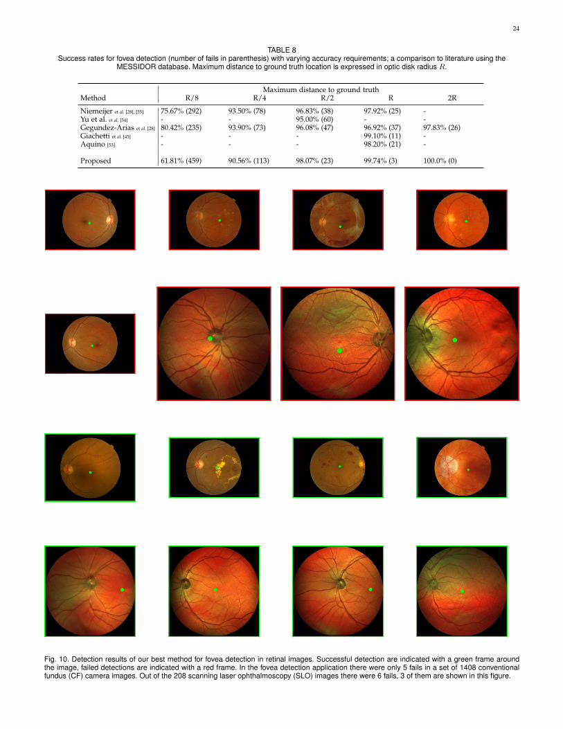
24

TABLE 8Success rates for fovea detection (number of fails in parenthesis) with varying accuracy requirements; a comparison to literature using the

MESSIDOR database. Maximum distance to ground truth location is expressed in optic disk radius R.

Maximum distance to ground truthMethod R/8 R/4 R/2 R 2R

Niemeijer et al. [28], [55] 75.67% (292) 93.50% (78) 96.83% (38) 97.92% (25) -Yu et al. et al. [54] - - 95.00% (60) - -Gegundez-Arias et al. [28] 80.42% (235) 93.90% (73) 96.08% (47) 96.92% (37) 97.83% (26)Giachetti et al. [45] - - - 99.10% (11) -Aquino [53] - - - 98.20% (21) -

Proposed 61.81% (459) 90.56% (113) 98.07% (23) 99.74% (3) 100.0% (0)

Fig. 10. Detection results of our best method for fovea detection in retinal images. Successful detection are indicated with a green frame aroundthe image, failed detections are indicated with a red frame. In the fovea detection application there were only 5 fails in a set of 1408 conventionalfundus (CF) camera images. Out of the 208 scanning laser ophthalmoscopy (SLO) images there were 6 fails, 3 of them are shown in this figure.

25

Fig. 11. Detection results of our best method for pupil detection. Successful detection are indicated with a green frame around the image, faileddetections are indicated with a red frame.

E.2 Results with Rotation and Scale Invariance

Here we perform rotation and scale invariant templatematching via the extension described in Subsec. E.1. Weselected the best template combination for each specificapplication and compared non-invariant template matching(as described in the main article) to rotation and/or scaleinvariant template matching (Subsec. E.1). The best templatecombination for ONH detection was AR2 + Clog:SE(2), forfovea detection this was Clin:R2 + Clog:SE(2), and for pupildetection this was Dlin:R2 + Elin:SE(2).

For the retinal applications we only tested for rotationinvariance with

α ∈ −π6,−π

8,− π

12,− π

24, 0,

π

24,π

12,π

8,π

6,

and did not included scale invariance since each retinalimage was already rescaled to a standardized resolution (seeSubsec. D.2.1). In pupil detection we tested for a range ofscalings with

a ∈ 0.7, 0.8, 0.9, 1.0, 1.1, 1.2, 1.3

to deal with varying pupil sizes caused by varying distancesto the camera; and we tested for a range of rotations with

α ∈ −π4,−π

8,− π

16, 0,

π

16,π

8,π

4

to deal with rotations of the head.

E.2.1 Detection ResultsThe detection results are shown in Table. 10. Here wecan see that in all three applications the inclusion of arotation/scale invariant matching scheme results in a slightdecrease in performance. This can be explained by the factthat variations in scale an rotation within the databasesare small, and that the trained templates can already dealrobustly with these variations (due to the presence of suchvariations in the training set). By introducing rotation/scaleinvariance one then only increases the likelihood of falsepositive detections.

E.2.2 Computation TimeThe effect on computation time of rotation/scale invariantmatching is shown in Fig. 12. Here one sees that compu-tation time linearly increases with the number of template

26

TABLE 9Average template matching results (± standard deviation) for pupildetection in 5-fold cross validation, number of failed detections in

parentheses. A successful detection has a normalized error e ≤ 0.1.

Template BioID (Full image) BioID (Periocular image)ID 1521 1521

R2 templates

AR2 41.03% ± 1.45% (897) 59.70% ± 1.52% (613)

Blin:R2 0.00% ± 0.00% (1521) 3.62% ± 1.09% (1466)Clin:R2 12.95% ± 2.22% (1324) 67.26% ± 2.55% (498)Dlin:R2 8.28% ± 1.80% (1395) 75.68% ± 2.33% (370)Elin:R2 11.51% ± 2.25% (1346) 71.47% ± 2.76% (434)

Blog:R2 0.00% ± 0.00% (1521) 0.00% ± 0.00% (1521)Clog:R2 12.89% ± 2.06% (1325) 39.91% ± 3.37% (914)Dlog:R2 1.84% ± 0.95% (1493) 22.09% ± 2.37% (1185)Elog:R2 10.39% ± 2.26% (1363) 37.21% ± 4.37% (955)

SE(2) templates

ASE(2) 57.72% ± 1.68% (643) 75.34% ± 1.31% (375)

Blin:SE(2) 8.74% ± 2.00% (1388) 41.81% ± 5.04% (885)Clin:SE(2) 84.61% ± 4.19% (234) 86.78% ± 3.68% (201)Dlin:SE(2) 85.53% ± 3.44% (220) 87.18% ± 3.71% (195)Elin:SE(2) 85.47% ± 3.82% (221) 87.11% ± 3.87% (196)

Blog:SE(2) 0.00% ± 0.00% (1521) 0.13% ± 0.29% (1519)Clog:SE(2) 86.52% ± 0.77% (205) 93.95% ± 1.33% (92)Dlog:SE(2) 75.21% ± 2.18% (377) 89.48% ± 2.27% (160)Elog:SE(2) 83.30% ± 1.68% (254) 92.77% ± 1.02% (110)

Template combinations (sorted on performance full image)∗Clin:R2 + Elin:SE(2) 93.49% ± 1.49% (99) 95.60% ± 1.46% (67)Clin:R2 +Dlin:SE(2) 93.16% ± 1.54% (104) 95.00% ± 1.15% (76)Elin:R2 + Elin:SE(2) 93.10% ± 1.04% (105) 95.59% ± 0.89% (67)Elin:R2 +Dlin:SE(2) 92.97% ± 1.62% (107) 95.27% ± 1.31% (72)Clin:R2 + Clin:SE(2) 92.70% ± 1.41% (111) 95.33% ± 0.97% (71)Elin:R2 + Clin:SE(2) 92.64% ± 0.94% (112) 95.33% ± 0.94% (71)Dlin:R2 +Dlin:SE(2) 92.51% ± 0.96% (114) 95.79% ± 0.82% (64)Dlin:R2 + Elin:SE(2) 92.24% ± 1.23% (118) 95.86% ± 0.89% (63)Elog:R2 +Dlin:SE(2) 92.11% ± 2.26% (120) 93.23% ± 1.93% (103)Dlin:R2 + Clog:SE(2) 92.05% ± 1.52% (121) 95.14% ± 0.78% (74)

... ...

Template combinations (sorted on performance periocular image)∗Dlin:R2 + Elin:SE(2) 92.24% ± 1.23% (118) 95.86% ± 0.89% (63)Dlin:R2 +Dlin:SE(2) 92.51% ± 0.96% (114) 95.79% ± 0.82% (64)Dlin:R2 + Clin:SE(2) 91.52% ± 1.25% (129) 95.73% ± 0.77% (65)Elin:R2 + Elin:SE(2) 93.10% ± 1.04% (105) 95.59% ± 0.89% (67)Clin:R2 + Elin:SE(2) 93.49% ± 1.49% (99) 95.60% ± 1.46% (67)Elin:R2 + Clin:SE(2) 92.64% ± 0.94% (112) 95.33% ± 0.94% (71)Clin:R2 + Clin:SE(2) 92.70% ± 1.41% (111) 95.33% ± 0.97% (71)Elin:R2 +Dlin:SE(2) 92.97% ± 1.62% (107) 95.27% ± 1.31% (72)Dlin:R2 + Elog:SE(2) 91.72% ± 1.23% (126) 95.27% ± 0.79% (72)Dlin:R2 + Clog:SE(2) 92.05% ± 1.52% (121) 95.14% ± 0.78% (74)

... ...† AR2 +ASE(2) 61.34% ± 1.54% (588) 68.18% ± 1.25% (484)

... ...∗Best template combination that does not rely on logistic regression.†Best template combination that does not rely on template optimization.

TABLE 10Average template matching results (± standard deviation, number of

fails between parenthesis) for optic nerve head (ONH), fovea, and pupildetection in 5-fold cross validation.

Method Success rate

ONH Detection (1737 images)

No invariance 99.83% ± 0.26% (3)Rotation invariance 99.60% ± 0.16% (7)

Fovea Detection (1616 images)

No invariance 99.32% ± 0.26% (11)Rotation invariance 97.10% ± 0.65% (47)

Pupil Detection (1521 images)

No invariance 95.86% ± 0.89% (63)Rotation invariance 94.48% ± 1.62% (84)Scale invariance 95.33% ± 1.46% (71)Rotation + scale invariance 94.28% ± 2.10% (87)

Fig. 12. Average computation times for the detection of one pupil/eyeper image, using SE(2) or R2 templates, testing for different templateorientations or scalings. Two experiments are shown, in blue the numberof template orientations Nα = 1 and the number of scalings Na isvaried, in orange-dashed the number of scalings Na = 1 and thenumber of rotations is Nα is varied.

rotations and scalings tested for. This timings-experimentis performed on the pupil detection application, and theshown timings are only of step 5 of the full detection pipeline(see Subsec. D.2.1 and Table 1) as this is the only step that isaffected by the rotation/scale invariant extension.

REFERENCES

[1] J.-C. Yoo and T. Han, “Fast normalized cross-correlation,” CSSP,vol. 28, no. 6, pp. 819–843, 2009.

[2] P. Viola and M. Jones, “Rapid object detection using a boostedcascade of simple features,” in CVPR 2001. Proceedings of the 2001IEEE Computer Society Conference on, vol. 1, 2001, pp. I–511–I–518.

[3] N. Dalal and B. Triggs, “Histograms of oriented gradients forhuman detection,” in CVPR 2005. IEEE Computer Society Conferenceon, vol. 1, June 2005, pp. 886–893.

[4] D. Lowe, “Object recognition from local scale-invariant features,”in Computer Vision, 1999. The Proceedings of the Seventh IEEE Inter-national Conference on, vol. 2, 1999, pp. 1150–1157 vol.2.

[5] H. Bay, T. Tuytelaars, and L. Van Gool, “Surf: Speeded up robustfeatures,” in ECCV 2006, ser. Lecture Notes in Computer Science,A. Leonardis, H. Bischof, and A. Pinz, Eds. Springer BerlinHeidelberg, 2006, vol. 3951, pp. 404–417.

27

[6] R. Duits, M. Felsberg, G. H. Granlund, and B. M. ter Haar Romeny,“Image analysis and reconstruction using a wavelet transformconstructed from a reducible representation of the euclidean mo-tion group,” IJCV, vol. 72, no. 1, pp. 79–102, 2007.

[7] E. Bekkers, R. Duits, T. Berendschot, and B. ter Haar Romeny,“A multi-orientation analysis approach to retinal vessel tracking,”JMIV, pp. 1–28, 2014.

[8] A. E. Hoerl and R. W. Kennard, “Ridge regression: Biased estima-tion for nonorthogonal problems,” Technometrics, vol. 12, no. 1, pp.55–67, 1970.

[9] J. Zhang, R. Duits, G. Sanguinetti, and B. M. ter Haar Romeny,“Numerical approaches for linear left-invariant diffusions on se(2),their comparison to exact solutions, and their applications inretinal imaging,” Numerical Mathematics: Theory, Methods and Ap-plications, vol. 9, pp. 1–50, 2 2016.

[10] R. Duits and E. Franken, “Left-invariant parabolic evolutions onSE(2) and contour enhancement via invertible orientation scorespart I: Linear left-invariant diffusion equations on SE(2),” Quar-terly of Applied Mathematics, vol. 68, no. 2, pp. 255–292, 2010.

[11] T. J. Hastie, R. J. Tibshirani, and J. H. Friedman, The elementsof statistical learning : data mining, inference, and prediction, ser.Springer series in statistics. New York: Springer, 2009, autresimpressions : 2011 (corr.), 2013 (7e corr.).

[12] M. Hebiri and S. van de Geer, “The smooth-lasso and other 1+2-penalized methods,” Electron J Stat, vol. 5, pp. 1184–1226, 2011.

[13] R. Cuingnet, J. Glaunes, M. Chupin, H. Benali, and O. Colliot,“Spatial and anatomical regularization of svm: A general frame-work for neuroimaging data,” Pattern Analysis and Machine Intelli-gence, IEEE Transactions on, vol. 35, no. 3, pp. 682–696, March 2013.

[14] H. Xu, C. Caramanis, and S. Mannor, “Robustness and regulariza-tion of support vector machines,” The Journal of Machine LearningResearch, vol. 10, pp. 1485–1510, 2009.

[15] A. A. Qazi, D. R. Jrgensen, M. Lillholm, M. Loog, M. Nielsen, andE. B. Dam, “A framework for optimizing measurement weightmaps to minimize the required sample size,” Medical Image Analy-sis, vol. 14, no. 3, pp. 255 – 264, 2010.

[16] C. Li and H. Li, “Network-constrained regularization and variableselection for analysis of genomic data,” Bioinformatics, vol. 24,no. 9, pp. 1175–1182, 2008.

[17] C. De Boor, “A practical guide to splines,” Math. Comp., 1978.[18] P. Green and B. Silverman, Nonparametric regression and generalized

linear models: a roughness penalty approach. CRC Press, 1993.[19] M. Unser, “Splines: a perfect fit for signal and image processing,”

Signal Processing Magazine, vol. 16, no. 6, pp. 22–38, Nov 1999.[20] M. Unser, A. Aldroubi, M. Eden, and L. Fellow, “B-spline signal

processing: Part i-theory,” IEEE TSP, vol. 41, pp. 821–833, 1993.[21] P. Thomas Fletcher, “Geodesic regression and the theory of least

squares on riemannian manifolds,” International Journal of Com-puter Vision, vol. 105, no. 2, pp. 171–185, 2013.

[22] N. Miolane and X. Pennec, “A survey of mathematical structuresfor extending 2D neurogeometry to 3D image processing,” inMICCAI-MVC, Munich, Germany, Oct. 2015.

[23] X. Pennec, “Intrinsic statistics on riemannian manifolds: Basictools for geometric measurements,” Journal of Mathematical Imagingand Vision, vol. 25, no. 1, pp. 127–154, 2006.

[24] R. Vidal, Y. Ma, and S. Sastry, “Generalized principal componentanalysis (gpca),” Pattern Analysis and Machine Intelligence, IEEETransactions on, vol. 27, no. 12, pp. 1945–1959, Dec 2005.

[25] O. Tuzel, F. Porikli, and P. Meer, “Learning on lie groups forinvariant detection and tracking,” in CVPR. IEEE, 2008, pp. 1–8.

[26] N. Patton, T. M. Aslam, T. MacGillivray, I. J. Deary, B. Dhillon,R. H. Eikelboom, K. Yogesan, and I. J. Constable, “Retinal imageanalysis: concepts, applications and potential,” Progress in retinaland eye research, vol. 25, no. 1, pp. 99–127, 2006.

[27] S. A. Ramakanth and R. V. Babu, “Approximate nearest neighbourfield based optic disk detection,” Computerized Medical Imaging andGraphics, vol. 38, no. 1, pp. 49 – 56, 2014.

[28] M. E. Gegundez-Arias, D. Marin et al., “Locating the fovea centerposition in digital fundus images using thresholding and featureextraction techniques,” Computerized Medical Imaging and Graphics,vol. 37, no. 56, pp. 386 – 393, 2013, retinal Image Analysis.

[29] D. W. Hansen and Q. Ji, “In the eye of the beholder: A surveyof models for eyes and gaze,” Pattern Analysis and Machine Intelli-gence, IEEE Transactions on, vol. 32, no. 3, pp. 478–500, 2010.

[30] R. Duits, M. Duits, M. Almsick, and B. Haar Romeny, “Invertibleorientation scores as an application of generalized wavelet the-ory,” PRIA, vol. 17, no. 1, pp. 42–75, 2007.

[31] E. Bekkers, R. Duits, and B. ter Haar Romeny, “Optic nerve headdetection via group correlations in multi-orientation transforms,”in Image Analysis and Recognition, ser. LNCS, A. Campilho andM. Kamel, Eds. Springer, 2014, pp. 293–302.

[32] E. Bekkers, R. Duits, and M. Loog, “Training of templates for objectrecognition in invertible orientation scores: Application to opticnerve head detection in retinal images,” in EMMCVPR. Springer,2015, pp. 464–477.

[33] G. Citti and A. Sarti, “A cortical based model of perceptualcompletion in the roto-translation space,” JMIV, vol. 24, no. 3, pp.307–326, 2006.

[34] R. Duits and B. Burgeth, “Scale spaces on lie groups,” in ScaleSpace and Variational Methods in Computer Vision, ser. Lecture Notesin Computer Science, F. Sgallari, A. Murli, and N. Paragios, Eds.Springer Berlin Heidelberg, 2007, vol. 4485, pp. 300–312.

[35] P. Craven and G. Wahba, “Smoothing noisy data with splinefunctions,” Num. Math., vol. 31, no. 4, pp. 377–403, 1978.

[36] F. O’sullivan, B. S. Yandell, and W. J. Raynor Jr, “Automaticsmoothing of regression functions in generalized linear models,”JASA, vol. 81, no. 393, pp. 96–103, 1986.

[37] C. Gu, “Cross-validating non-gaussian data,” Journal of Computa-tional and Graphical Statistics, vol. 1, no. 2, pp. 169–179, 1992.

[38] D. Xiang and G. Wahba, “A generalized approximate cross val-idation for smoothing splines with non-gaussian data,” StatisticaSinica, vol. 6, pp. 675–692, 1996.

[39] S. Lu and J. Lim, “Automatic optic disc detection from retinalimages by a line operator,” Biomedical Engineering, IEEE TBME,vol. 58, no. 1, pp. 88–94, 2011.

[40] A. Aquino, M. E. Geg, and D. Mar, “Automated optic disk de-tection in retinal images of patients with diabetic retinopathy andrisk of macular edema,” IJBLS, vol. 8, no. 2, pp. 87–92, 2012.

[41] B. Dashtbozorg, A. M. Mendona, and A. Campilho, “Optic discsegmentation using the sliding band filter,” Computers in Biologyand Medicine, vol. 56, pp. 1 – 12, 2015.

[42] S. Sekhar, F. E. Abd El-Samie, P. Yu, W. Al-Nuaimy, and A. K.Nandi, “Automated localization of retinal features.” Applied Op-tics, vol. 50, no. 19, pp. 3064–75, 2011.

[43] D. Marin, M. E. Gegundez-Arias et al., “Obtaining optic disccenter and pixel region by automatic thresholding methods onmorphologically processed fundus images,” Computer Methods andPrograms in Biomedicine, vol. 118, no. 2, pp. 173 – 185, 2015.

[44] H. Yu et al., “Fast localization and segmentation of optic disk inretinal images using directional matched filtering and level sets.”IEEE TITB, vol. 16, no. 4, pp. 644–57, 2012.

[45] A. Giachetti, L. Ballerini, E. Trucco, and P. Wilson, “The useof radial symmetry to localize retinal landmarks,” ComputerizedMedical Imaging and Graphics, vol. 37, no. 56, pp. 369 – 376, 2013,retinal Image Analysis.

[46] A. Youssif et al., “Optic disc detection from normalized digitalfundus images by means of a vessels’ direction matched filter.”IEEE TMI, vol. 27, no. 1, pp. 11–8, 2008.

[47] M. Foracchia et al., “Luminosity and contrast normalization inretinal images.” MEDIA, vol. 9, no. 3, pp. 179–90, 2005.

[48] J. Bruna and S. Mallat, “Invariant scattering convolution net-works,” IEEE transactions on pattern analysis and machine intelli-gence, vol. 35, no. 8, pp. 1872–1886, 2013.

[49] W. Freeman and E. Adelson, “The design and use of steerablefilters,” IEEE TPAMI, vol. 13, no. 9, pp. 891–906, Sep 1991.

[50] A. Aquino, M. E. Gegundez-Arias, and D. Marin, “Detecting theoptic disc boundary in digital fundus images using morphological,edge detection, and feature extraction techniques,” IEEE TMI,vol. 29, no. 11, pp. 1860–9, 2010.

[51] S. Lu, “Accurate and efficient optic disc detection and segmenta-tion by a circular transformation,” IEEE TMI, vol. 30, no. 12, pp.2126–2133, Dec 2011.

[52] M. Abramoff and M. Niemeijer, “Mass screening of diabeticretinopathy using automated methods,” in Teleophthalmology inPreventive Medicine, G. Michelson, Ed. Springer, 2015, pp. 41–50.

[53] A. Aquino, “Establishing the macular grading grid by means offovea centre detection using anatomical-based and visual-basedfeatures,” Comp. in Biology and Medicine, vol. 55, pp. 61 – 73, 2014.

[54] H. Yu, S. Barriga, C. Agurto, S. Echegaray et al., “Fast localizationof optic disc and fovea in retinal images for eye disease screening,”Proc. SPIE, vol. 7963, pp. 796 317–796 317–12, 2011.

[55] M. Niemeijer, M. D. Abramoff, and B. van Ginneken, “Fast de-tection of the optic disc and fovea in color fundus photographs.”MEDIA, vol. 13, no. 6, pp. 859–70, 2009.

28

[56] M. Leo, D. Cazzato, T. De Marco, and C. Distante, “Unsupervisedeye pupil localization through differential geometry and local self-similarity matching,” PloS one, vol. 9, no. 8, p. e102829, 2014.

[57] N. Markus, M. Frljak, I. S. Pandzic, J. Ahlberg, and R. Forchheimer,“Eye pupil localization with an ensemble of randomized trees,”Pattern recognition, vol. 47, no. 2, pp. 578–587, 2014.

[58] B. Kroon, A. Hanjalic, and S. M. Maas, “Eye localization for facematching: is it always useful and under what conditions?” inProceedings of the 2008 international conference on Content-based imageand video retrieval. ACM, 2008, pp. 379–388.

[59] S. Asteriadis, N. Nikolaidis, and I. Pitas, “Facial feature detectionusing distance vector fields,” Pattern Recognition, vol. 42, no. 7, pp.1388–1398, 2009.

[60] P. Campadelli, R. Lanzarotti, and G. Lipori, “Precise eye andmouth localization,” International Journal of Pattern Recognition andArtificial Intelligence, vol. 23, no. 03, pp. 359–377, 2009.

[61] F. Timm and E. Barth, “Accurate eye centre localisation by meansof gradients.” in VISAPP. SciTePress, 2011, pp. 125–130.

[62] R. Valenti and T. Gevers, “Accurate eye center location throughinvariant isocentric patterns,” Pattern Analysis and Machine Intelli-gence, IEEE Transactions on, vol. 34, no. 9, pp. 1785–1798, 2012.

[63] K. Yosida, “Resolvent and spectrum,” in Functional Analysis, ser.Classics in Mathematics. Springer Berlin Heidelberg, 1995, vol.123, pp. 209–231.

[64] L. Hormander, “Hypoelliptic second order differential equations,”Acta Mathematica, vol. 119, no. 1, pp. 147–171, 1967.

[65] E. P. Hsu, Stochastic analysis on manifolds. American MathematicalSoc., 2002, vol. 38.