Journal paper accepted - Tim Menzies

International Journal of Software Engineering and Knowledge Engineering

! World Scientific Publishing Company

1

EXPLORING THE EFFORT OF GENERAL SOFTWARE PROJECT

ACTIVITIES WITH DATA MINING

TOPI HAAPIO

Lane Department of Computer Science, West Virginia University,

Morgantown, WV 26506-610, USA

[email protected]

TIM MENZIES

Lane Department of Computer Science, West Virginia University,

Morgantown, WV 26506-610, USA

[email protected]

Accepted Mar 29, 2011

Software project effort estimation requires high accuracy, but accurate estimations are difficult to

achieve. Increasingly, data mining is used to improve an organization’s software process quality, e.g.

the accuracy of effort estimations. Data is collected from projects, and data miners are used to

discover beneficial knowledge. This paper reports a data mining experiment in which we examined

32 software projects to improve effort estimation. We examined three major categories of software

project activities, and focused on the activities of the category which has got the least attention in

research so far, the non-construction activities. The analysis is based on real software project data

supplied by a large European software company. In our data mining experiment, we applied a range

of machine learners. We found that the estimated total software project effort is a predictor in

modeling and predicting the actual quality management effort of the project.

Keywords: Effort estimation; data mining; project behavior.

1. Introduction

A software supplier organization strives to estimate as accurately as possible the effort

needed in building software to ensure that the project’s adherence to budget and

schedules, and the successful allocation of resources [1]. A vast number of approaches,

techniques and tools have been developed for both modeling and estimating software

project effort. Although these approaches take various factors into account, the general

software project activities which are not directly related to software construction or

project management have not been considered to be one of the major effort categories. In

contrast, effort estimation research and applications focus on software construction,

because the majority of the total effort is software construction effort [2][3]. For instance,

the well-known work breakdown structures [2][4][5][6] overlook general software

project activities [7]. However, the amount of effort related to general software project

activities can be greater than the project management effort and also can vary remarkably

2 Haapio, T. and Menzies, T.

between projects [8]. Can the overlooked general software project activities and their

effort be a reason for the high effort estimation inaccuracy (in [8], the median magnitude

of relative error (MdMRE) was reported to be 0.34)?

In this study, we experimented with data mining to assess the impact of non-

construction activities compared with other software project activities on effort estimates.

Our data mining experiment results (presented in sub-section 3.2.1) are two-fold: whereas

we find no evidence that general software project activities are a significant factor

influencing effort estimation, we find evidence of a relation between the estimated total

software project effort and the actual effort of one of the general software project

activities, namely quality management. This finding can be used in improving effort

estimations, and is a useful supplement to the scanty research on the possible impacts of

effort estimates on project work and behavior [9].

The remainder of this paper is structured as follows. Section 2 describes the

theoretical background of this study and presents our prior work on defining general

software project activities as a group called ‘non-construction activities’. The data mining

experiment with interpretation of the results are presented in Section 3. Finally, Section 4

offers a short summary.

2. Related and Prior Work

In this section, we present the theoretical background to this study and our prior work

related to the general software project activities.

2.1. Theoretical background

The theoretical background of this work is two-fold. On the one hand, there are the key

concepts of the research domain: effort and its estimation, effort distribution and work

breakdown structure. On the other hand, there is the research approach used for achieving

our goal to improve effort estimate accuracy: experimenting by data mining.

2.1.1. Key concepts

The effort of a software project can be generally defined as the time consumed by the

project, and it can be expressed as a number of person hours, days, months or years,

depending on the size of the project. The effort is estimated in most projects. An estimate

is a probabilistic assessment with a reasonably accurate value of the center of a range.

Formally, an estimate is defined as the median of the (unknown) distribution [10]. An

estimate is a prediction; hence, an estimation model can be considered to be a prediction

system. Indeed, software project effort is one of the most-modeled software engineering

areas. The most widely known formal modeling approaches include the regression-based

composite models COCOMO (Constructive Cost Model) [2] and COCOMO II [4][11].

However, the most widely used empirical effort estimation technique in practice is expert

judgment, particularly because there is no conclusive evidence that a formal approach

outperforms the informal expert analysis [12].

Exploring the Effort of General Software Project Activities 3

Although effort can be distributed in a project between project activities or project

phases in many different ways, effort distribution is a less-investigated effort estimation

area. Indeed, it has been disputed whether it is useful to distribute effort in the first place

[3], although examples exist in the software engineering literature; Brooks' suggestion for

rule-of-thumb effort distribution for software construction was one of the first in the mid-

1970s [13]. Effort is distributed on software project activities that together form a work

breakdown structure, WBS. A WBS is a particular defined tree-structure hierarchy of

elements that decomposes the project into discrete work tasks that can be scheduled and

prioritized, and used for project budgetary planning and control purposes [2][6][14][15].

A WBS is also required by the currently employed capability maturity models, e.g.

CMMI [16]. However, no standardized way to create a WBS exists, and the software

engineering literature provides only a few general WBS including ones applied with the

two COCOMO models [2][4], the Rational Unified Process (RUP) activity distribution

[6], and the ISO/IEC 12207 work breakdown structure for software life-cycle processes

[5]. The topic is largely avoided in the published literature because the development of a

WBS depends on numerous project-specific parameters [6].

2.1.2. Experimenting and data mining

In this study, we employ experimenting [17][18] as our research methodology. In a

controlled experiment, as many factors as possible belonging to the studied phenomenon

are under researcher’s control [19]. Suppositions, assumptions, speculations and beliefs

are tested with experimenting. In other words, the purpose of experimentation is to match

ideas with reality [18].

Experimentations have two levels [18]: the first level is experimenting in laboratory

(controlled conditions), and the second level is experimenting in reality (uncontrolled

conditions), i.e. experimentation is carried out with real projects. The tightness of control

is, however, usually in opposition to the richness of reality at the same level of

knowledge [19]. Subsequently, the researchers have to ultimately make a trade-off

between these two iso-epistemic attributes.

In a controlled experiment, the Goal/Question/Metric paradigm provides a useful

framework [17]. In the Goal/Question/Metric (GQM) paradigm [20], data collection is

designed thus [21]:

(1) Conceptual level (Goal): a goal is defined for an object for a variety of reasons, with

respect to various models of quality, from various points of view and relative to a

particular environment.

(2) Operational level (Question): a set of questions is used to define models of the object

of study and then focuses on that object to characterize the assessment or

achievement of a specific goal.

(3) Quantitative level (Metric): a set of metrics, based on the models, is associated with

every question in order to answer it in a measurable way.


One of the techniques used to achieve goals in a controlled experiment is data mining.

Data mining is also one of the popular processes for producing business intelligence (BI)

information, which is utilized in improving the software process quality of cost or effort

estimations, for instance. Data mining is used to reveal hidden patterns in unstructured

data to provide valuable information for business utilization. Indeed, BI and data mining

have been increasingly employed in the software industry for finding predictors from data

for modeling software project effort. The data mining tools are employed to model the

data [22] by regression or with trees, for example. The models of data behavior are

generated with data mining learners, using appropriate data. The data can be gathered

either manually or automatically. On a general level, project data collection can be

divided into two groups according to its purpose: the data which is collected during a

project for the project’s own purposes, and the data which is collected from multiple

projects for BI and software process improvement (SPI) purposes. Whereas the

automated data gathering processes can produce a vast amount of data in some business

areas [22], manual data gathering results usually in smaller and noisier data sets. Another

reason for the differences in data set sizes and quality is that in non-commercial

organizations government funding can enable a more research-motivated and extensive

data collection, whereas in the software industry data collection is more driven by the

customer needs and the process maturity models which the companies are committed to.

2.2. Prior work: defining the non-construction activities

In 2003, the quality executives at Tieto Corporation were concerned about the effects of

software project activities other than actual software construction and project

management ones on both software project effort and effort estimation accuracy, i.e.

these general software project activities had not had the attention they might have

required. The management hypothesized that focusing only on software construction and

project management in effort estimations while neglecting or undervaluing other project

activities can result in inaccurate estimates. Accordingly, in this experiment, we explore

these general software project activities that could affect effort estimates.

In [8], we noted that much of the effort estimation work focuses on the first two of

the three parts of a software project WBS:

(1) Software construction involves the effort needed for the actual software construction

in the project’s life-cycle frame, such as analysis, design, implementation, and

testing. Without this effort, the software cannot be constructed, verified and

validated for the customer hand-over.

(2) Project management involves activities that are conducted solely by the project

manager, such as project planning and monitoring, administrative tasks, and

steering group meetings.

(3) All the general software project activities in the project’s life-cycle frame that do not

belong to the other two main categories can be termed non-construction activities.


These include various management and support activities, which are carried out by

several members of the project.

In [7][8], we developed the taxonomy shown in Figure 1 by applying the grounded

theory methodology [23]. In brief, we employed a three-step grounded theory method

which involved firstly gathering the data sample of 26 software projects (a subset of the

data set used in this study), followed by defining the main software project activity

categories and deciding upon the one for generating the WBS, and finally coding the

activities within the non-construction activity category, including identifying and

extracting the activities from the data, renaming the activities, and categorizing them

iteratively into logic entities [7].

Fig. 1. Software project activity breakdown structure with three major categories and further decomposed non-

construction activities.

The activity extraction of the non-construction activity category resulted in seven

individual, but generic, software project activities [7]:

(1) Configuration management. Configuration management (CM), or software

configuration management (SCM), is the development and application of standards

and procedures for managing an evolving system product [1]. In other words, SCM

is a set of umbrella activities that have been developed to manage change throughout

the life-cycle of software [24]. These activities include CM planning, identification

of objects in the software configuration, management and control of change, versions

and releases, system building, configuration auditing, and reporting. We also include

the management of the technical surroundings of the software in CM [7].

(2) Customer-related activities. The customer-related activities (e.g. customer inquiries,

support, and training) include activities having interactions with customers and end-

users.


(3) Documentation. Documentation includes all other documentation than software

construction (analysis or design) documentation, e.g. system documentation,

manuals, standards etc.

(4) Orientation. Orientation is the transfer of knowledge about a software’s business

domain, technology etc. to a project group member, i.e. all learning activities

involved with the particular project. These activities usually take place at the

beginning of the project before it can be considered to be input and thus a part of

some construction activity, e.g. software design.

(5) Project-related activities. All activities related to the functionality of a particular

project as an organization (software team, or project team or group) are included in

this category, e.g. project events and project team meetings.

(6) Quality management. Quality management (QM) is an umbrella activity consisting

of the management and assurance of quality, and including the reviews of

documentation and software code [1][24]. In simple terms, QM involves defining

the procedures and standards which should be used during software development

and checking that these have been followed [1]. QM has three principal activities:

quality assurance, quality planning, and quality control. Quality assurance (QA)

defines a framework for achieving software quality [1]. QA consists of a set of

auditing and reporting functions that assess the effectiveness and completeness of

quality control activities such as formal technical reviews [24] or peer inspections

[6].

(7) Miscellaneous activities. Project-specific, individual activities are included in the

miscellaneous activities category. These activities include time for traveling and

sales efforts, for instance.

3. Experiment

In our experiment, we employ data mining techniques to find predictors for the effort of

different project activities. The data mining experiment aims at assessing the impact of

non-construction activities compared with other software project activities. The learners

used in data mining are presented in sub-section 3.1.2 and come from the Weka toolkit

software [25].

Data sets are created using both types of activities passed to a data miner. It should be

noted that if an activity is not useful in predicting some target class, it will not appear in

the model generated by the data miner. As we shall see, many activities will not prove to

be useful. With one exception, we do not remove variables a priori. Instead, we use data

mining experiments to determine which variables do not add significantly to the learning.

In this way, we can assert that removing those variables does not adversely affect the

variables. Our single exception to this rule is the “miscellaneous activities” variable

which has the follow undesirable property: for the data sets we were dealing with, this

variable was used as a ‘dump’ category to record information that did not fit into any of

the other categories.


We report our experiment in the following two sub-sections. The first sub-section

reports both the experimental design and the execution of the experiment. In the second

sub-section, we present, analyze and interpret our results.

3.1. Experimental design and execution

3.1.1. Variables

For practical reasons (i.e. to be performed in the software engineering industry), we

define variables that are common and related to most software projects, and that are

available and used in effort estimating at the beginning of the project. Our predictors

(also called, independent variables or inputs [17]) include project, organization, customer,

size (in terms of estimated effort), and non-construction activity related variables:

• Project variables

• ReqAnalysisPriorEstimation. A dichotomous predictor indicating whether the

project had a requirements analysis phase prior to effort estimation. Intuitively,

this might increase the amount of orientation effort since more documentation is

available.

• Type. A categorical predictor indicating that the project type is either

‘Development’ (something new is going to be built) or ‘Enhancement’ (an

existing system is enhanced with new features). Intuitively, an enhancement

project does not require as much non-construction activity effort as a

development project because variables such as customer, business domain,

technical environment etc. are known.

• Technology. A categorical predictor with the values ‘Java_J2EE’,

‘ClientServer_TM’, and ‘Other’, indicating which technology was employed in

the project. In our data set, the projects are mainly either Java/J2EE projects, or

client/server projects employing a transaction monitor with Windows clients. A

few projects applied other technologies. The organization in question has longer

experience of client/server projects than of Java/J2EE, which emerged during

the first decade of the 2000. Does a new technology have an impact on non-

construction activity effort?

• Organization variables

• TE_Team. A nominal predictor with a value indicating the name of the project

team which constructed and manpowered the project. Does the fact that the

teams differ from each other, for example in terms of their skills, have an impact

on non-construction activity effort?

• Customer variables

• Customer. A nominal predictor with a value indicating customer’s name.

Customers have an impact on effort, or do they? For example, the organization

in question has longer experience of one of the customers than of the others.

Also, customers vary in terms of their software engineering process maturity.

• CustomerBusinessDomain. A categorical predictor with the value

‘TelecomOperator’, ‘Telecom’ or ‘Government’. The customer’s business


domain has an impact on effort, or does it? Telecom customers tend to have

more experience of IT, IT projects and software engineering, whereas

government customers usually buy these as services. Also, the organization in

question has longer experience of the telecom operator business domain than the

others.

• Size (in terms of estimated effort) variables

• LogEstimatedEffort. A ratio predictor with a logarithmic value of estimated

effort in hours. Because the projects could not been distributed equally based on

their size in terms of effort, we applied a logarithm transformation into the

variable of estimated effort before letting the Weka application [25] learn a

model. It is common to take the logarithms of effort values to transform a model

into a linear model [10][26]. The effort extraction had two main phases: the

calculation of effort needed for the three main categories, and the calculation of

effort for each non-construction activity. First, the proportions of effort needed

for software construction, project management, and non-construction activities

were calculated. Effort data was gathered from the work time registry system

into which the project personnel feed their work hours for different project-

specific activities at half-hour precision. The activities along with their effort

inputs were reorganized into the three categories according to the definition

given in sub-section 2.2. Second, the effort proportions of each non-construction

activity were calculated.

• ConsideredAsASmallProject_Md. A categorical predictor with the value ‘Small’

or ‘Large’. Projects were divided into two groups according to the median

estimated effort (1999.8 h) value of the 32 projects (under=’Small’,

over=’Large’).

• ChaosSizeConsidered. A categorical predictor with the value ‘Small’ or ‘Large’.

Projects were divided into two groups according to the Standish definition of a

small project (6 persons * 6 months * 150 h/month = 5400 h, estimated effort)

[27].

• Non-construction activity variables

• Number_NCA_Activities. A ratio predictor indicating the number of registration

entries of non-construction activities created in the time-booking system’s work

breakdown structure.

• NCAEntitiesOfAll. A ratio predictor indicating the percentage of registration

entries of non-construction activities of all registration entries.

Our response variables (also called dependent or output variables [17][28]) is a set of

continuous classes representing the actual effort proportions of the three major software

project categories (software construction, project management, non-construction

activities) and six further decomposed non-construction activities:

(1) SC_Effort_Percent,

(2) PM_Effort_Percent,

(3) NCA_Effort_Percent,

(4) ConfigurationManagement_Percent,


(5) CustomerRelatedActivities_Percent,

(6) Documentation_Percent,

(7) Orientation_Percent,

(8) ProjectRelatedActivities_Percent,

(9) QualityManagement_Percent.

As noted in section 3, we exclude the ‘miscellaneous activities’ response class for

two reasons: firstly, the frequency of these activities appearing in a project is small

compared with the frequencies of the other activities [7], and secondly, ‘miscellaneous

activities’, with no common denominator, is a ‘dump’ category.

3.1.2. Data mining: process and tool

Our data mining experiment will have two or three steps, depending on the success of the

second step. First, we apply Feature Subset Selection (FSS) prior to the next steps of

learning, encouraged by the results of other studies (e.g. [26][29]). We employ FSS to

analyze the predictors before classifying them. A repeated result in the data mining

community is that simpler models with equivalent or higher performance can be built via

FSS algorithms that intelligently prune useless variables (or, columns or features) [29].

Variables may be pruned for several reasons:

• they may be noisy, i.e. contain spurious signals unrelated to the target class,

• they may be uninformative, e.g. contain mostly one value, or no repeating values,

• they may be correlated to other variables, in which case, they can be pruned since

their signal is also present in other variables.

A reduced variable set has many advantages:

• Models containing fewer variables generally have less variance in their outputs [30].

• The smaller the model, the fewer are the demands on interfaces (sensors and

actuators) to the external environment. Hence, systems designed around small

models are easier to use (less to do) and cheaper to build.

• In terms of this paper, the most important aspect of learning from a reduced variable

set is that it produces smaller models. Such smaller models are easier to explain (or

audit).

We utilize the FSS results in creating subsets of variables by pruning the variables

that do not receive a high number of folds. These pruned subsets assist us to gain the best

results in data mining with the different learners.

In FSS, we apply Weka’s Wrapper Feature Subset Selection, based on Kohavi and

John’s Wrapper algorithm [31], in the process, since experiments by other researchers

(e.g. [29]) strongly suggest that it is superior to many other variable pruning methods.

Starting with the empty set, Wrapper adds some combinations of variables and asks a

target learner to build a model using just those variables. Wrapper then grows the set of


selected variables and checks if a better model comes from learning over the larger set of

variables.

Second, after FSS, we apply learners for continuous classes. Besides having a long

and widespread history, the linear models can perform well when the data is sparse,

despite being simple and naïve [32].

We will interpret our results with the fit of the linear model which is expressed in

terms of the correlation coefficient. In a ‘perfect’ result (i.e. the linear model fits

perfectly), the coefficient would be a magnitude of 1, and in an ‘acceptable’ result for us

the coefficient would be over |0.6000|.

If the results are not acceptable (i.e. too small correlation coefficients), we continue

and (third) discretize the classes and apply the learners for discrete classes, encouraged

by Witten and Frank, who note that “even methods that can handle numeric attributes

often produce better results, or work faster, if the attributes are prediscretized” [33] (p.

287).

In our experiment, we attempt to develop statistical models to predict software project

activity effort. The variables related to the project, organization, customer, size (in terms

of estimated effort) and non-construction activity serve as predictors. The discretized

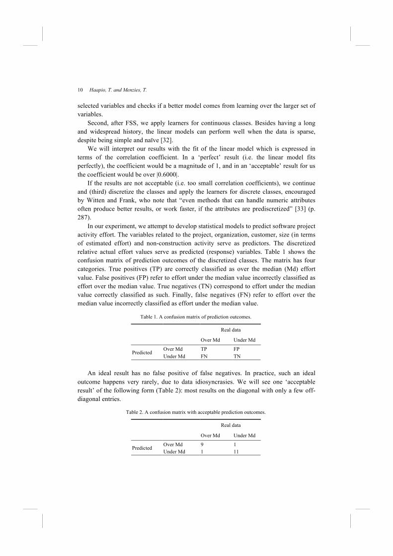
relative actual effort values serve as predicted (response) variables. Table 1 shows the

confusion matrix of prediction outcomes of the discretized classes. The matrix has four

categories. True positives (TP) are correctly classified as over the median (Md) effort

value. False positives (FP) refer to effort under the median value incorrectly classified as

effort over the median value. True negatives (TN) correspond to effort under the median

value correctly classified as such. Finally, false negatives (FN) refer to effort over the

median value incorrectly classified as effort under the median value.

An ideal result has no false positive of false negatives. In practice, such an ideal

outcome happens very rarely, due to data idiosyncrasies. We will see one ‘acceptable

result’ of the following form (Table 2): most results on the diagonal with only a few off-

diagonal entries.

Table 1. A confusion matrix of prediction outcomes.

Real data

Over Md Under Md

Over Md TP FP Predicted

Under Md FN TN

Table 2. A confusion matrix with acceptable prediction outcomes.

Real data

Over Md Under Md

Over Md 9 1 Predicted

Under Md 1 11


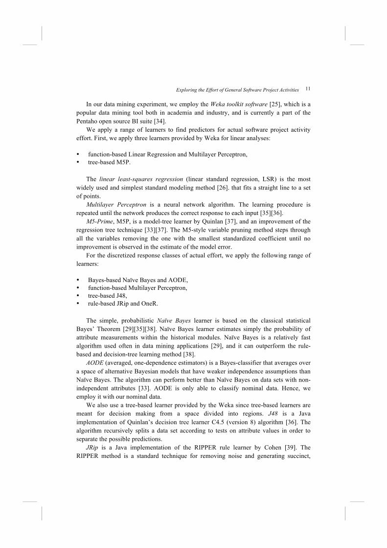
In our data mining experiment, we employ the Weka toolkit software [25], which is a

popular data mining tool both in academia and industry, and is currently a part of the

Pentaho open source BI suite [34].

We apply a range of learners to find predictors for actual software project activity

effort. First, we apply three learners provided by Weka for linear analyses:

• function-based Linear Regression and Multilayer Perceptron,

• tree-based M5P.

The linear least-squares regression (linear standard regression, LSR) is the most

widely used and simplest standard modeling method [26]. that fits a straight line to a set

of points.

Multilayer Perceptron is a neural network algorithm. The learning procedure is

repeated until the network produces the correct response to each input [35][36].

M5-Prime, M5P, is a model-tree learner by Quinlan [37], and an improvement of the

regression tree technique [33][37]. The M5-style variable pruning method steps through

all the variables removing the one with the smallest standardized coefficient until no

improvement is observed in the estimate of the model error.

For the discretized response classes of actual effort, we apply the following range of

learners:

• Bayes-based Naïve Bayes and AODE,

• function-based Multilayer Perceptron,

• tree-based J48,

• rule-based JRip and OneR.

The simple, probabilistic Naïve Bayes learner is based on the classical statistical

Bayes’ Theorem [29][35][38]. Naïve Bayes learner estimates simply the probability of

attribute measurements within the historical modules. Naïve Bayes is a relatively fast

algorithm used often in data mining applications [29], and it can outperform the rule-

based and decision-tree learning method [38].

AODE (averaged, one-dependence estimators) is a Bayes-classifier that averages over

a space of alternative Bayesian models that have weaker independence assumptions than

Naïve Bayes. The algorithm can perform better than Naïve Bayes on data sets with non-

independent attributes [33]. AODE is only able to classify nominal data. Hence, we

employ it with our nominal data.

We also use a tree-based learner provided by the Weka since tree-based learners are

meant for decision making from a space divided into regions. J48 is a Java

implementation of Quinlan’s decision tree learner C4.5 (version 8) algorithm [36]. The

algorithm recursively splits a data set according to tests on attribute values in order to

separate the possible predictions.

JRip is a Java implementation of the RIPPER rule learner by Cohen [39]. The

RIPPER method is a standard technique for removing noise and generating succinct,


easily explainable models from data. RIPPER’s covering algorithm runs over the data in

multiple passes. Rule-covering algorithms learn one rule at each pass for the majority

class. All the examples that satisfy the conditions are marked as covered and removed

from the data set. The algorithm then recourses on the remaining data. RIPPER is useful

for generating very small rule sets.

Holte’s OneR [40], or 1R, algorithm builds prediction rules using one or more values

from a single attribute. OneR takes as input a set of examples, each with several attributes

and a class. Its goal is to infer a rule that predicts the class given the values of the

attributes. It selects one-by-one attributes from a data set and generates a different set of

rules based on the error rate from the training set. Finally, the OneR algorithm chooses

the most informative single attribute (the one that offers rules with minimum error) and

bases the rule on this attribute alone in constructing the final decision tree [35][40][41].

3.1.3. Data collection, preparation, quality, and visualization

In this sub-section, we introduce our data and address our adherence to the data

preparation guidelines presented by Pyle [22][28]. The guidelines are applied whenever

possible. However, Pyle’s guidelines on choosing data are, in our view, meant for a large

data source and for choosing sample records from the large source, not a small data set

such as ours. In our case, we use project data that we had access to in 2003-2008, and

which had sufficient and relevant data. Although there are hundreds of projects on-going

in the company in question, most of the project data is inaccessible for confidentiality

reasons or not usable for data mining purposes because of the poor data quality.

The experiment is based on sample of real software project data supplied by a

software company, Tieto Finland Oy, a part of Tieto Corporation, which is one of the

largest IT services companies in northern Europe, with 17,000 employees.

The data set consists of 32 custom software development and enhancement projects,

which took place in 1999-2006. These projects were delivered to five different Nordic

customers who operate mainly in the telecommunication business domain. The delivered

software systems were based on different technical solutions. However, the two most

common technologies were based either on J2EE or on transaction management-based

client/server technology. The duration of the projects was between 1.9 and 52.8 months.

The projects, which were carried out by different teams within the same Finnish business

division, required an effort of between 276.5 and 51,426.6 person hours.

The median effort of software construction, project management and non-

construction activities in the 32 software projects are 76.7%, 11.3%, and 11.2%,

respectively. The box-plot presentation of the effort of these major software activity

categories showing the minimum and maximum, and the first and third quartile values, is

presented in Figure 2.


Fig. 2. The effort of software construction, project management, and non-construction activities (N=32).

The median effort of software construction does not differ from that reported by

MacDonell and Shepperd (76.7% and 76.9%, respectively) [3], although their approach

and basis of division were different to ours. This suggests that there might be a tendency

to have a certain effort distribution, and that the division in this study seems to be

appropriate. Also, it is notable that in this data set the non-construction activity effort

proportion is very similar to that of the project management. However, as seen in Figure

2, the deviation of this effort proportion between projects is significant. Both non-

construction activity effort amount and variance suggests that it is important to view the

non-construction activities and their effort as an independent group.

All the projects used a waterfall-like software development process, since iterative

and agile processes have emerged in more recent projects. The project process life-cycle

started from either the analysis phase or the design phase. All projects ended in customer

acceptance of delivery. This span forms the project’s life-cycle frame, which was quite

typical for delivery software projects in this organization. The normal work iteration is

included in the effort data. Effort caused by change requests, however, is excluded from

the data used for both predictor and response classes because the work caused by change

requests is not initially known and is therefore not included in the original effort

estimation. For this experiment, the information related to the effort estimates is gathered

from the tender proposal documents, the contract documents, and the final report

documents. Originally, projects’ efforts were estimated by using the expert judgment

estimation technique in every project. Function Point Analysis was used in some projects

as a secondary method to support the results. The actual effort data was gathered from the

time-booking system prior to the experiment. The project team members enter their effort

in this system.

In the guidelines for data preparation, Pyle notes that the collected records should be

distributed into three representative data sets: training, testing, and evaluation [22][28].

Due to our small data set this requirement is unreasonable. Instead, we perform the data


mining with one single data set, using a 2/3rd, 1/3rd train/test cross-validation procedure,

repeated ten times.

Pyle also gives instructions on missing values and data translations [22][28]. We

manipulate our data as little as possible: for example, all missing values are left out and

are not replaced by a mean or median value. The values for effort estimate in hours are

recalculated as logarithms, which is the usual method [10][26], and further derived to two

predictors (ConsideredAsASmallProject_Md, ChaosSizeConsidered) representing

estimated effort.

Following Pyle’s guidelines [22][28], we first visualized the data (the predictors in

respect to each response) using Weka’s visualizing features (Figure 3), including

cognitive nets (Figure 4), also to referred as cognitive maps [22]. However, no eminent

predictor for responses could be found by applying these visualizing methods.

Fig. 3. Data visualization with Weka (predictors for quality management effort).


Fig. 4. The cognitive (Bayes) net data visualization for the non-construction activity effort.

3.2. Analysis and interpretation

3.2.1. Results

In this sub-section, we report our findings resulting from the three data mining steps in

which we apply first the Feature Subset Selection, then learners for continuous classes,

and finally learners for discretized classes.

Our FSS uses ten-fold cross-validation for accuracy estimation. The selection search

is used to produce a list of attributes to be used for classification. Attribute selection is

performed using the training data and the corresponding learning schemes for each

machine learner. We find that the Wrapper performs better on discrete classes than on

continuous classes. We give two examples of our FSS results below; Table 3 shows the

results for Linear Regression for continuous classes, and Table 4 shows Naïve Bayes for

discrete classes.

Table 3. Number of folds (>=5) in 10-fold cross-validation for continuous classes.

Variable SC PM NCA Con Cus Doc Ori Pro Qua Mean

Project variables

ReqAnalysisPriorEstimation - - - - - - - 8 - 8

Type - - 10 - - - - - - 10

Technology - - - - - - - - - -

Organization variables

TE_Team - - 7 - - - - - - 7

Customer variables

Customer - - 8 - - - - - - 8

CustomerBusinessDomain - - - - - - - - - -

Size (effort) variables

ConsideredAsASmallProject_Md - - - - 9 - - - 8 8.5


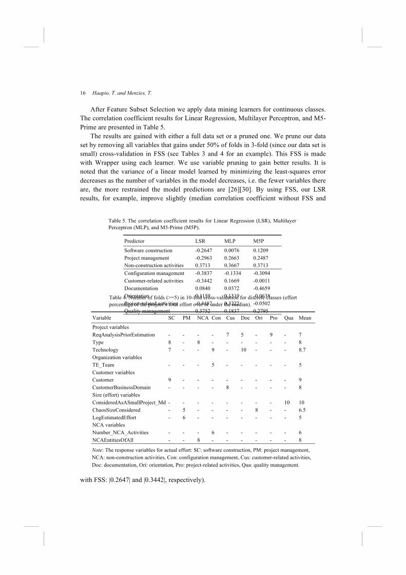
After Feature Subset Selection we apply data mining learners for continuous classes.

The correlation coefficient results for Linear Regression, Multilayer Perceptron, and M5-

Prime are presented in Table 5.

The results are gained with either a full data set or a pruned one. We prune our data

set by removing all variables that gains under 50% of folds in 3-fold (since our data set is

small) cross-validation in FSS (see Tables 3 and 4 for an example). This FSS is made

with Wrapper using each learner. We use variable pruning to gain better results. It is

noted that the variance of a linear model learned by minimizing the least-squares error

decreases as the number of variables in the model decreases, i.e. the fewer variables there

are, the more restrained the model predictions are [26][30]. By using FSS, our LSR

results, for example, improve slightly (median correlation coefficient without FSS and

with FSS: |0.2647| and |0.3442|, respectively).

Table 4. Number of folds (>=5) in 10-fold cross-validation for discrete classes (effort

percentage of the project’s total effort over or under the median).

Variable SC PM NCA Con Cus Doc Ori Pro Qua Mean

Project variables

ReqAnalysisPriorEstimation - - - - 7 5 - 9 - 7

Type 8 - 8 - - - - - - 8

Technology 7 - - 9 - 10 - - - 8.7

Organization variables

TE_Team - - - 5 - - - - - 5

Customer variables

Customer 9 - - - - - - - - 9

CustomerBusinessDomain - - - - 8 - - - - 8

Size (effort) variables

ConsideredAsASmallProject_Md - - - - - - - - 10 10

ChaosSizeConsidered - 5 - - - - 8 - - 6.5

LogEstimatedEffort - 6 - - - - - - - 5

NCA variables

Number_NCA_Activities - - - 6 - - - - - 6

NCAEntitiesOfAll - - 8 - - - - - - 8

Note: The response variables for actual effort: SC: software construction, PM: project management,

NCA: non-construction activities, Con: configuration management, Cus: customer-related activities,

Doc: documentation, Ori: orientation, Pro: project-related activities, Qua: quality management.

Table 5. The correlation coefficient results for Linear Regression (LSR), Multilayer

Perceptron (MLP), and M5-Prime (M5P).

Predictor LSR MLP M5P

Software construction -0.2647 0.0076 0.1209

Project management -0.2963 0.2663 0.2487

Non-construction activities 0.3713 0.3667 0.3713

Configuration management -0.3837 -0.1334 -0.3094

Customer-related activities -0.3442 0.1669 -0.0011

Documentation 0.0840 0.0372 -0.4659

Orientation 0.1159 0.1319 -0.0638

Project-related activities -0.4487 0.3222 -0.0502

Quality management 0.3752 0.1837 0.2795


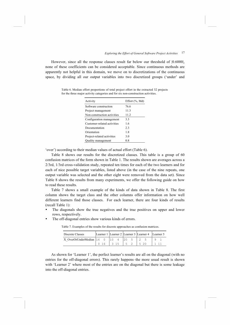
However, since all the response classes result far below our threshold of |0.6000|,

none of these coefficients can be considered acceptable. Since continuous methods are

apparently not helpful in this domain, we move on to discretizations of the continuous

space, by dividing all our output variables into two discretized groups (‘under’ and

‘over’) according to their median values of actual effort (Table 6).

Table 8 shows our results for the discretized classes. This table is a group of 60

confusion matrices of the form shown in Table 1. The results shown are averages across a

2/3rd, 1/3rd cross-validation study, repeated ten times for each of the two learners and for

each of nice possible target variables, listed above (in the case of the nine repeats, one

output variable was selected and the other eight were removed from the data set). Since

Table 8 shows the results from many experiments, we offer the following guide on how

to read these results.

Table 7 shows a small example of the kinds of data shown in Table 8. The first

column shows the target class and the other columns offer information on how well

different learners find those classes. For each learner, there are four kinds of results

(recall Table 1):

• The diagonals show the true negatives and the true positives on upper and lower

rows, respectively.

• The off-diagonal entries show various kinds of errors.

As shown for ‘Learner 1’, the perfect learner’s results are all on the diagonal (with no

entries for the off-diagonal errors). This rarely happens–the more usual result is shown

with ‘Learner 2’ where most of the entries are on the diagonal but there is some leakage

into the off-diagonal entries.

Table 6. Median effort proportions of total project effort in the extracted 32 projects

for the three major activity categories and for six non-construction activities.

Activity Effort (%, Md)

Software construction 76.6

Project management 11.3

Non-construction activities 11.2

Configuration management 3.3

Customer-related activities 1.6

Documentation 2.3

Orientation 1.8

Project-related activities 3.0

Quality management 0.8

Table 7. Examples of the results for discrete approaches as confusion matrices.

Discrete Classes Learner 1 Learner 2 Learner 3 Learner 4 Learner 5

X_OverOrUnderMedian 16 0 10 4 20 5 2 5 9 1

0 16 3 15 5 2 5 20 1 11


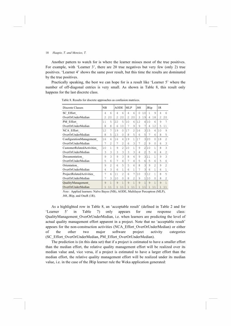
Another pattern to watch for is where the learner misses most of the true positives.

For example, with ‘Learner 3’, there are 20 true negatives but very few (only 2) true

positives. ‘Learner 4’ shows the same poor result, but this time the results are dominated

by the true positives.

Practically speaking, the best we can hope for is a result like ‘Learner 5’ where the

number of off-diagonal entries is very small. As shown in Table 8, this result only

happens for the last discrete class.

As a highlighted row in Table 8, an ‘acceptable result’ (defined in Table 2 and for

‘Learner 5’ in Table 7) only appears for one response class:

QualityManagement_OverOrUnderMedian, i.e. when learners are predicting the level of

actual quality management effort apparent in a project. Note that no ‘acceptable result’

appears for the non-construction activities (NCA_Effort_OverOrUnderMedian) or either

of the other two major software project activity categories

(SC_Effort_OverOrUnderMedian, PM_Effort_OverOrUnderMedian).

The prediction is (in this data set) that if a project is estimated to have a smaller effort

than the median effort, the relative quality management effort will be realized over its

median value and, vice versa, if a project is estimated to have a larger effort than the

median effort, the relative quality management effort will be realized under its median

value, i.e. in the case of the JRip learner rule the Weka application generated:

Table 8. Results for discrete approaches as confusion matrices.

Discrete Classes NB AODE MLP J48 JRip 1R

SC_Effort_ 4 6 4 6 4 6 0 10 1 9 4 6

OverOrUnderMedian 2 20 2 20 2 20 3 19 4 18 2 20

PM_Effort_ 11 5 22 5 10 6 12 4 10 6 9 7


NCA_Effort_ 12 7 19 0 17 2 16 3 15 4 10 9


ConfigurationManagement_ 16 4 16 4 19 1 17 3 20 0 18 2


CustomerRelatedActivities_ 10 1 9 2 10 1 9 2 10 1 8 3


Documentation_ 9 3 9 3 8 4 9 3 11 1 9 3


Orientation_ 9 2 6 5 5 6 8 3 9 2 9 2


ProjectRelatedActivities_ 7 6 11 2 6 7 10 3 12 1 8 5


QualityManagement_ 9 1 9 1 9 1 9 1 9 1 9 1


Note: Applied learners: Naïve Bayes (NB), AODE, Multilayer Perceptron (MLP),

J48, JRip, and OneR (1R).


(ConsideredAsASmallProject_Md = Small) =>

QualityManagement_OverOrUnderMedian=Over_Md (10.0/1.0)

=> QualityManagement_OverOrUnderMedian=Under_Md

(12.0/1.0)

The JRip rule tells that with the categorical predictor variable

ConsideredAsASmallProject_Md both categories of quality management effort response

variable (over and under median value) are classified correctly having only one

incorrectly classified case in both categories in the data set.

In other words, the predicted effort proportion of actual quality management effort is

larger in projects that are estimated in total as small rather than large ones.

3.2.2. Implications for research

Because of the small and noisy data set, our data mining experiment was not without

challenges. These challenges and how we overcame them are described as a case study in

another publication [42]. It is insightful to contrast our data mining experiment with the

guidelines proposed for experimenting in software engineering (e.g. [17][21][43]). It can,

in fact, be useful to allow for a redirection, halfway through a study. Just because a data

set does not provide answers to question X does not mean it cannot offer useful

information about question Y. Hence, we advise tuning the question to the data and not

the other way around. This advice is somewhat at odds with the guidelines presented in

the empirical software engineering literature (e.g. [17][21][43]), which advises tuning

data collection according to the goals of the study. In an ideal case, we can follow the

three steps of GQM. However, in the 21st century, the pace of change in both software

industry and software engineering organizations in general can make this impractical, as

it did in the NASA Software Engineering Laboratory (SEL), for instance. With the shift

from in-house production to outsourced, external contractors and production, and without

an owner of the software development process, each project could adopt its own

structure. The earlier SEL learning organization experimentation became difficult since

there was no longer a central model to build on [44].

The factors that led to the demise of the SEL are still active. Software engineering

practices are quite diverse, with no widely accepted or widely adopted definition of ‘best’

practices. The SEL failed because if could not provide value-added when faced with

software projects that did not fit their preconceived model of how a software project

should be conducted. In the 21st century, we should not expect to find large uniform data

sets where fields are well-defined and filled-in by the projects. Rather, we need to find

ways for data mining to be a value-added service, despite idiosyncrasies in the data.

Consequently, we recommend GQM when data collection can be designed before a

project starts its work. Otherwise, as done in this study, we recommend using data mining

as a microscope to closely examine data. While it useful to start such a study with a goal

in mind, an experimenter should be open to stumbling over other hypotheses. Sometimes,

experiments run as expected, but often the unexpected finding (“that’s strange”) can be


more informative than rigidly following a plan that was determined before there was any

feedback from the particular data set.

One drawback with our exploratory exercise could be susceptible to “shotgun

correlation” effects (the detection of spurious connections between randomly generated

variables) [45]. Hence, we offer the conclusions below as working hypotheses that (a)

require monitoring within an organization and (b) could be disproved by further

observations.

In this regard, our conclusions have the same status as other scientific hypotheses.

Popper argues that no conclusion is absolute and that all conclusions require monitoring,

lest future data requires that the conclusions be changed [46]. Our conclusions are as

valid as those in any other field where we cannot control the phenomenon being studied,

but can only observe it.

Finally, we note that if we do not apply our methods to generate conclusions then we

may lose valuable insights. The study was originally designed as a regression analysis on

historical data. When that failed, we could have stopped. However, had we done so, we

would have had to dismiss a data set that had been very hard and expensive to collect.

Despite the small size of our data set, it represented the entirety of the cross-project

corporate experience gained up until this point. If we were to ignore the potential insights

it contains, that experience could have been lost.

3.2.3. Implications for practice

The practical implication of this study relate to the specific conclusion we can offer to

software businesses and quality management. The implication is that the actual quality

management (QM) effort proportion of total project effort will be larger in projects that

are estimated to be small rather than large, which has to be considered in the effort

estimates.

Intuitively, absolute QM effort increases with project size and total effort, as there are

more project deliverables requiring quality assurance. Indeed, our data shows such a

tendency between the absolute effort values of quality management and total project

effort. However, our data does not support a pattern of a linear, logarithmic or

exponential growth of quality management effort as the total effort of a project increases.

This implies that quality management effort is not a constant in software projects and

thus cannot be predicted with an approach applying merely a constant. In fact, this

supports the findings for quality assurance effort behavior in software projects (cf. Figure

V.24 in [47] (p. 419)).

We can conclude that we can set a maximum proportion for QM effort as a rule-of-

thumb when estimating the QM effort for large projects. In a tight market situation, the

correct smallest possible estimate of the QM cost could improve the chances of winning a

deal. However, the rule-of-thumb does not hold for smaller projects. It seems that in

small projects we can set a minimum proportion for the QM effort but the actual amount

can turn out larger.


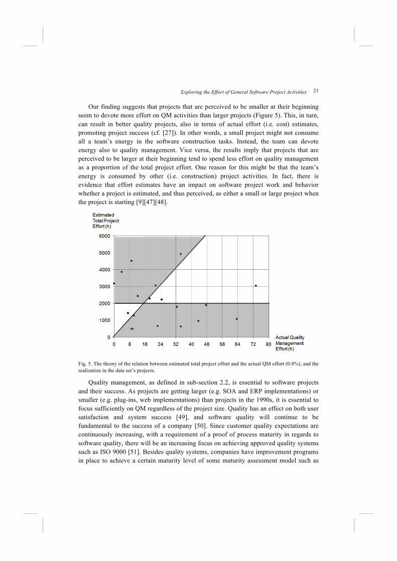
Our finding suggests that projects that are perceived to be smaller at their beginning

seem to devote more effort on QM activities than larger projects (Figure 5). This, in turn,

can result in better quality projects, also in terms of actual effort (i.e. cost) estimates,

promoting project success (cf. [27]). In other words, a small project might not consume

all a team’s energy in the software construction tasks. Instead, the team can devote

energy also to quality management. Vice versa, the results imply that projects that are

perceived to be larger at their beginning tend to spend less effort on quality management

as a proportion of the total project effort. One reason for this might be that the team’s

energy is consumed by other (i.e. construction) project activities. In fact, there is

evidence that effort estimates have an impact on software project work and behavior

whether a project is estimated, and thus perceived, as either a small or large project when

the project is starting [9][47][48].

Fig. 5. The theory of the relation between estimated total project effort and the actual QM effort (0.8%), and the

realization in the data set’s projects.

Quality management, as defined in sub-section 2.2, is essential to software projects

and their success. As projects are getting larger (e.g. SOA and ERP implementations) or

smaller (e.g. plug-ins, web implementations) than projects in the 1990s, it is essential to

focus sufficiently on QM regardless of the project size. Quality has an effect on both user

satisfaction and system success [49], and software quality will continue to be

fundamental to the success of a company [50]. Since customer quality expectations are

continuously increasing, with a requirement of a proof of process maturity in regards to

software quality, there will be an increasing focus on achieving approved quality systems

such as ISO 9000 [51]. Besides quality systems, companies have improvement programs

in place to achieve a certain maturity level of some maturity assessment model such as


ISO/IEC 15504 [5] or CMMI [16] to meet both current and potential customer

expectations. Moreover, the cost of poor quality will be measured in most software

companies because quality becomes a key goal in improving the profitability and long-

term survival of the company [50]. Furthermore, the verification of software components

will become increasingly important, as software development is speeded up and the time-

to-market is shortened, and concurrently there is a need to verify the correctness of the

components [50].

In the light of our data mining experiment, QM was the only non-construction

activity that showed a pattern of estimated total project effort influencing actual effort.

One reason for this might be that QM (or its sub-activities) is intuitively considered

important by the project team, and is performed whenever possible (when a team’s

energy is not consumed by software construction). The other supporting activities (e.g.

configuration management, orientation, and documentation) do not present the same kind

of behavior, i.e. no pattern could be found in our data. However, on average in the

projects, all the other non-construction activities consumed more effort than QM, which

indicates that they are necessary in a software project (cf. [7]). Moreover, these activities

are relevant for the success of the delivery in terms of both software and project quality,

and thus should not be considered a cost overhead. Devoting effort to non-construction

activities can indeed reduce the effort needed for software construction or project

management, and reduce the cost of poor quality in terms of, for example, warranty costs.

Hence, all non-construction activities must be carefully considered in software project

effort estimation, but unfortunately our data does not reveal to what extent, except for the

QM effort.

3.2.4. Limitations of study

We consider the limitations of this study in regards to two aspects: general limitations

related to software project effort data and the threats to the validity of an experiment.

This study suffers from general limitations related to the data. These limitations are

typical for software industry effort-related studies. The general concern related to the data

is the reliability of the actual effort. As project group members feed their own work hours

into the time-booking system, there can be individual variations with the inputs.

Moreover, project group members can be too embarrassed to enter all the non-

construction activity time (e.g. orientation, problem solving, planning, waiting). On the

other hand, they may dump all unclear or non-billable project effort on some non-

construction activity. Also, if these activities were not created as registration entries in

the time-booking system, no effort could be fed to the activity. This means either that the

effort was not registered at all, or it was fed to another activity (usually some software

construction activity), which skews the effort data. Furthermore, the work hours were

entered with half-hour precision, which also skews the data. Also, Hochstein et al. note

that the effort recorded varies significantly depending on whether it is automated

(instrumented) or self-recorded [52]. Hence, self-recorded effort is never quite reliable.


The threats to the validity of an experiment can be distributed in four groups [17]:

conclusion, internal, construct, and external validity. Conclusion validity addresses the

significance of the results. Measured in term of conclusion validity, our conclusions are

quite strong: the use of 10 cross-validation experiments ensures that our results hold over

multiple samples of the data. Internal validity addresses the causality between the

variables. The causal nature of our conclusions was discussed in sub-section 3.2.3. In that

sub-section, we noted that we can infer a reasonable causal explanation for our result

(that smaller projects may have the mistaken belief that their projects need less quality

management). Construct validity addresses the relation between the theory and

observation. In general, construct validity is very difficult to assess in software

engineering since there are so few established theories. Recent catalogues of software

engineering knowledge report that most of that knowledge is yet to reach the theory

stage. For example, Endres and Rombach proposed a view of how knowledge gets built

about software and systems engineering [53]. They distinguish between:

• observations of what actually happens during development in a specific context can

happen all the time (‘observation’ in this case is defined to comprise both hard facts

and subjective impressions),

• recurring observations that lead to laws that help understand how things are likely to

occur in the future,

• laws are explained by theories that explain why those events happen.

While [53] lists over a hundred laws, they mention no theories. That is, it is hard to

assess the construct validity of our conclusions since there are so few reference theories

that we can cite which are relevant to this work. External validity addresses the

generalization of the results into practice. This is a data mining experiment and, as such,

the status of our conclusions should be clearly stated. We assess our methods using

across-validation technique that checks how well models perform on data not used during

training. Hence, our conclusions are only certified on the train/test data used in this study.

These conclusions could be refuted if some future study found better methods than the

methods proposed here. The reader may protest this approach since it does not seek

generalizable truths that hold in all projects. In reply, we note that:

• there are very few (if any) examples of such universal causal theories in the software

engineering literature (cf. [53]),

• one value-added feature of data mining is that it is an automated process.

In addition, a concern related to the generalization of the results, is that the data is

provided by only one company and one of its business divisions. However, since the

project settings and the project methods varied between teams and the 32 projects, the

data sample represents a heterogenic project environment. Moreover, the data sample

presents real software projects, which were carried out in software industry to real

customers.


Järvinen notes that the scientific rigorous of an experiment correlates with the number

of factors used in it [19]. We experimented with a limited set of factors but, on the other

hand, might gain more relevant and applicable results with natural like experimental

setting (cf. [19]). We experimented in uncontrolled conditions in reality, i.e. the

experimentation was carried out with real projects.

It can be concluded that that most threats relate to the software project effort data.

However, as this is a universal problem with industry effort data, this was accepted for

this research. To increase the reliability of the results, replications of this experiment with

a larger data set of within-company and cross-company data will endeavor to not only

confirm our findings but also to make new predictor findings in regards to non-

construction activities. Whereas this study is limited to quantitative research, a qualitative

survey or case study among project team members could partly verify our assumption

concerning a team’s energy devoted to quality management, i.e. why teams reduce their

effort on quality management in projects that are perceived to be large, and how the

project team apprehends the importance of quality management over other non-

construction activities.

3.2.5. Lessons learned

A further lesson learned for data mining is that some machine learners perform better

than others. However, no consistent superior learner was found. Hence, we recommend

that in a data mining experiment it is advantageous to apply several learners since

different learners perform best for different response classes. This, naturally, is more

time-consuming than employing only one superior learner, which must be acknowledged

also by corporate organizations which demand immediate results. However, the nature of

knowledge discovery in databases (KDD) should be iterative [54], i.e. the results and

learning can be obtained by trial-and-error. In our case, we started with linear models

before moving todiscretized data and learners, as suggested by the FSS.

Some interpretations of learner performance can be made: for continuous classes,

Linear Regression outperforms M5-Prime and Multilayer Perceptron. For discrete

classes, all discrete learners perform equally in the case of our only ‘acceptable’ finding.

A similar finding was reported by Dougherty et al. when they observed that the

performance of classifiers such as Naïve Bayes usually improved after converting

continuous variables to discrete variables [55].

4. Conclusions

In this study, we sought for predictors of software project activity effort as a part of a

project aiming to construct practical improvements to effort estimations. In particular, we

focus on the general software project activities. These non-construction activities together

comprise an amount of effort in software projects equal to that of project management,

and thus should be acknowledged in effort estimations.

Our main conclusion for the software engineering research is that the question must

be tuned to the data. In the modern diverse and outsourced software engineering world,


many of the premises of prior software engineering research no longer hold. We cannot

assume a static sweet-structured domain where consistent data can be collected from

multiple projects over many years for research and other utilizing purposes. We need to

recognize that data collection has it limits in organizations driven by minimizing costs,

and customers being the main stakeholder for data collection reason. Thus, we conclude

with a recommendation to analyze the initial stand-point for data mining, and then either

continue with GQM or, as in our case, use data mining for data examination.

Our main finding for the software engineering practice, which should be considered

in effort estimations, concerns one of the non-construction activities. Our data mining

results suggest that the amount of a project’s estimated effort is a predictor of the actual

quality management effort: the proportion of quality management effort is larger in

projects where the total estimated project effort is smaller rather than larger. Although

our finding concerns the smallest non-construction activity effort proportion in our data

set, in the software industry all findings that can improve effort estimations and the

accuracy of the effort estimates are considered relevant and welcome. In addition, this

research supplements the scanty research on the possible impacts of effort estimates on

project work and behavior.

Our finding of the pattern in quality management effort data would have remained

hidden without data mining. Thus, we can recommend data mining in analyzing industry

effort data even if the data set in hand is noisy and small. In addition, we found that some

machine learners perform better than others, and learners for discretized classes

outperformed learners for continuous classes. Also, the results can be improved by using

Feature Subset Selection prior to learning.

Acknowledgments

The authors would like thank Prof. Anne Eerola, of the University of Eastern Finland, for

commenting on the draft paper, and V. Michael Paganuzzi, of the University of Eastern

Finland, for his linguistic advice. The first author is grateful to the Nokia Foundation for

the Nokia Scholarship he received to conduct this study at WVU.

References

[1] I. Sommerville, Software Engineering (6th ed., Pearson Education, Harlow, UK, 2001).

[2] B. Boehm, Software Engineering Economics (Prentice Hall, Englewood Cliffs, NJ, 1981).

[3] S. MacDonell and M. Shepperd, Using prior-phase effort records for re-estimation during

software projects, In Proc. 9th Int. Software Metrics Symposium (METRICS'03), Sydney,

Australia, 2003, pp. 1-13.

[4] B. Boehm, C. Abts, A.W. Brown, S. Chulani, B.K. Clark, E. Horowitz, R. Madachy, D.

Reifer, and B. Steece, Software Cost Estimation with COCOMO II (Prentice-Hall, Upper

Saddle River, NJ, 2000).

[5] ISO, ISO/IEC 12207, Information Technology - Software Life Cycle Processes. ISO, 1995.

[6] W. Royce, Software Project Management: A Unified Framework (Addison-Wesley, Reading,

MA, 1998).


[7] T. Haapio, Generating a Work Breakdown Structure: A Case Study on the General Software

Project Activities, in Proc. 13th European Conf. on European Systems & Software Process

Improvement and Innovation (EuroSPI'2006), Joensuu, Finland, 2006, 11.1-11.

[8] T. Haapio, The Effects of Non-Construction Activities on Effort Estimation, in Proc. 27th

Information Systems Research in Scandinavia (IRIS’27), Falkenberg, Sweden, 2004.

[9] M. Jørgensen and D. Sjøberg, Impact of effort estimates on software project work,

Information and Software Technology 43(15) (2001) 939-948.

[10] N.E. Fenton and S.L. Pfleeger, Software Metrics: A Rigorous & Practical Approach (2nd ed.,

PWS Publishing Company, Boston, MA, 1997).

[11] B. Boehm, B. Clark, E. Horowitz, E. Westland, R. Madachy, and R. Selby, Cost Models for

Future Life Cycle Processes: COCOMO 2, Annals of Software Engineering 1(1) (1995) 57-

94.

[12] M. Jørgensen, Estimation of software development work effort: evidence on expert judgement

and formal model, International Journal of Forecasting 3(3) (2007) 449–462.

[13] F.P. Brooks, Jr., The Mythical Man-Month. Essays on Software Engineering (Addison-

Wesley Publishing Company, Reading, MA, 1975).

[14] R. Agarwal, M. Kumar, Y.S. Mallick, R. Bharadwaj, and D. Anantwar, Estimating software

projects, ACM SIGSOFT Software Engineering Notes 26(4) (2001) 60-67.

[15] D. Wilson and M. Sifer, Structured planning-project views, Software Engineering Journal

3(4) (1988) 134-140.

[16] SEI, CMMI for Development, Version 1.2, CMMI-DEV, V1.2. Technical Report CMU/SEI-

2006-TR-008, ESC-TR-2006-008, CMU/SEI, 2006.

[17] C. Wohlin, P. Runeson, M. Höst, M. Ohlsson, B. Regnell, and A. Wesslén, Experimentation

in Software Engineering: An Introduction (Kluwer Academic Publishers, Boston, MA, 2000).

[18] N. Juristo and A. Moreno, Basics of Software Engineering Experimentation (Kluwer

Academic Publishers, Boston, MA, 2001).

[19] P. Järvinen, On Research Methods (Opinpajan kirja, Tampere, Finland, 2001).

[20] V. Basili and H. Rombach, The TAME Project: Towards Improvement-Oriented Software

Environments, IEEE Trans. on Software Engineering 14(6) (1988) 758-773.

[21] R. van Solingen and E. Berghout, The Goal/Question/Metric Method (McGraw-Hill

Education, London, UK, 1999).

[22] D. Pyle, Data Preparation for Data Mining (Morgan Kaufmann Publishers, Inc., San

Francisco, CA, 1999).

[23] B. Glaser and A. Strauss, Discovery of Grounded Theory: Strategies for Qualitative Research

(Aldine Transaction, Chicago, IL, 1967).

[24] R.S. Pressman, Software Engineering: A Practioner’s Approach (6th ed., McGraw-Hill, New

York, 2005).

[25] G. Holmes, A. Donkin, and I.H. Witten, WEKA: A Machine Learning Workbench, in Proc.

1994 Second Australian and New Zealand Conf. on Intelligent Information Systems, Brisbane,

Australia, 1994, pp. 357-361.

[26] Z. Chen, T. Menzies, D. Port, and B. Boehm, Finding the Right Data for Software Cost

Modeling, IEEE Software 22(6) (2005) 38-46.

[27] The Standish Group, Chaos: A Recipe for Success, 1999, www.standishgroup.com/

sample_research/PDFpages chaos1999.pdf.

[28] D. Pyle, Data Collection, Preparation, Quality, and Visualization, in The Handbook of Data

Mining, ed. N. Ye. (Lawrence Erlbaum Associates, Inc., 2003), pp. 365-391.

[29] M. Hall and G. Holmes, Benchmarking attribute selection techniques for discrete class data

mining, IEEE Trans. on Knowledge and Data Engineering 15(6) (2003) 1437-1447.

[30] A. Miller, Subset Selection in Regression (2nd ed., Chapman & Hall/CRC, Boca Raton,

2002).


[31] R. Kohavi and G.H. John, Wrappers for feature subset selection, Artificial Intelligence 97(1-

2) (1997) 273-324.

[32] G. Ridgeway, Strategies and Methods for Prediction, in The Handbook of Data Mining, ed. N.

Ye. (Lawrence Erlbaum Associates, Inc., 2003), pp. 159-191.

[33] I.H. Witten and E. Frank, Data Mining: Practical machine learning tools and techniques

(Morgan Kaufmann, Los Altos, CA, 2005).

[34] M. Hall, E. Frank, G. Holmes, B. Pfahringer, P. Reutemann, and I.H. Witten, The WEKA

data mining software: an update, SIGKDD Explorations Newsletter 11(1) (2009) 10-18.

[35] S. Ali and K.A. Smith, On learning algorithm selection for classification, Applied Soft

Computing 6(2) (2006) 119-138.

[36] R. Quinlan, C4.5: Programs for Machine Learning (Morgan Kaufmann, San Meteo, CA,

1992).

[37] R.J. Quinlan, Learning with Continuous Classes, in Proc. 5th Australian Joint Conf. on

Artificial Intelligence, Hobart, Tasmania, 1992, pp. 343-348,

http://citeseer.nj.nec.com/quinlan92learning.html.

[38] T. Menzies, J. Greenwald, and A. Frank, Data Mining Static Code Attributes to Learn Defect

Predictors, IEEE Trans. on Software Engineering 33(1) (2007) 2-13.

[39] W.W. Cohen, Fast Effective Rule Induction, in Proc. 12th Int. Conf. on Machine Learning,

Tahoe City, CA, USA, 1995, pp. 115-123,

http://citeseerx.ist.psu.edu/viewdoc/summary?doi=10.1.1.50.8204.

[40] R.C. Holte, Very simple classification rules perform well on most commonly used dataset,

Machine Learning 11 (1993) 63-91.

[41] C.G. Nevill-Manning, G. Holmes, and I.H. Witten, The Development of Holte’s 1R

Classifier, in Proc. Second New Zealand Int. Two-Stream Conf. on Artificial Neural Networks

and Expert Systems, Dunedin, New Zealand, 1995, pp. 239-242.

[42] T. Haapio and T. Menzies, Data Mining with Software Industry Data: A Case Study, in Proc.

IADIS Int. Conf. Applied Computing 2009 (AC’2009), Rome, Italy, 2009, pp. 33-38.

[43] B. Kitchenham, H. Al-Khilidar, M. Ali Babar, M. Berry, K. Cox, J. Keung, F. Kurniawati, M.

Staples, H. Zhang, and L. Zhu, Evaluating Guidelines for Empirical Software Engineering

Studies, in Proc. 2006 ACM/IEEE Int. Symposium on Empirical Software Engineering

(ISESE'06), Rio de Janeiro, Brazil, 2006, pp. 38-47.

[44] V. Basili, F. McGarry, R. Pajerski, and M. Zelkowitz, Lessons learned from 25 years of

process improvement: the rise and fall of the NASA software engineering laboratory, in Proc.

24th Int. Conf. on Software Engineering (ICSE’02), Orlando, USA, 2002, pp. 69-79.

[45] R. Courtney and D. Gustafson, Shotgun Correlations in Software Measures, Software

Engineering Journal 8(1) (1992) 5-11.

[46] K. Popper, Conjectures and Refutations: The Growth of Scientific Knowledge (Routledge &

Kegan Paul, London, UK, 1963).

[47] T. Abdel-Hamid, The dynamics of software development project management : an integrative

system dynamics perspective, Ph.D. thesis, Massachusetts Institute of Technology

Cambridge, MA, 1984, (pp. 410-427.

http://dspace.mit.edu/bitstream/handle/1721.1/38235/12536707.pdf?sequence=1.

[48] T. Abdel-Hamid and S. Madnick, Special Feature: Impact of Schedule Estimation on

Software Project Behavior, IEEE Software 3(4) (1986) 70-75

[49] M. Koivisto, Development of Quality Expectations in Mobile Information Systems, in Proc.

Int. Joint Conf. on Computer, Information, and Systems Sciences, and Engineering,

University of Bridgeport, CT, USA, 2007, pp. 336-341.

[50] G. O’Regan, A Practical Approach to Software Quality (Springer-Verlag New York, Inc.,

Secaucus, NJ, 2002).

[51] ISO, Quality management and quality assurance standards, ISO, 1994.


[52] L. Hochstein, V.R. Basili, M.V. Zelkowitz, J.K. Hollingsworth, and J. Carver, Combining

self-reported and automatic data to improve programming effort measurement, in Proc. 10th

European software engineering conf. held jointly with 13th ACM SIGSOFT int. symposium on

Foundations of software engineering, Lisbon, Portugal, 2005, pp. 356-365.

[53] A. Endres and H.D. Rombach, A Handbook of Software and Systems Engineering (Addison-

Wesley, Boston, MA, 2003).

[54] U. Fayyad, G. Piatetsky-Shapiro, and P. Smyth, The KDD process for extracting useful

knowledge from volumes of data, Comm. of the ACM 39(11) (1996) 27-34.

[55] J. Dougherty, R. Kohavi, and M. Sahami, Supervised and unsupervised discretization of

continuous features. In Proc. Twelfth Int. Conf. on Machine Learning, 1995, pp. 194-202.

Documents

Journal paper accepted - Tim Menzies