To only be used with a Demonstration version of JPCalcWin

The original MS-DOS C++ JPCalc versions were developed by Dr P H Barry (see Ref 5 in References and Further Reading). An earlier 16-bit Windows JPCalcW conversion was produced by Axon Instruments, Inc. (now part of Molecular Devices Corporation, USA), in conjunction with P H Barry.

This JPCalcWin version was redeveloped for 32/64-bit Windows by E Crawford (School of Medical Sciences, UNSW, Sydney, Australia), working from revised and extended MS-DOS C++ JPCalc source code, in consultation with P H Barry.

JPCalcWin

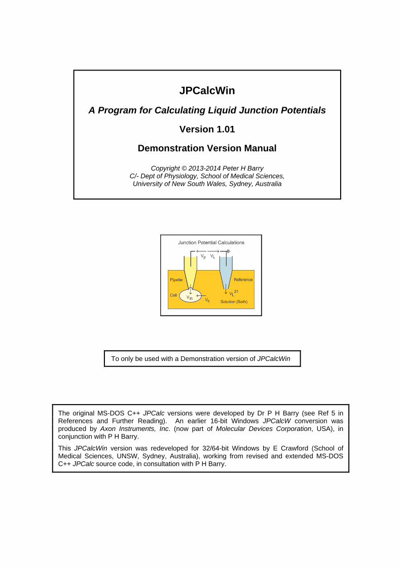
A Program for Calculating Liquid Junction Potentials

Version 1.01

Demonstration Version Manual

Copyright © 2013-2014 Peter H Barry C/- Dept of Physiology, School of Medical Sciences, University of New South Wales, Sydney, Australia

2

JPCalcWin Demonstration Version Users’ Manual

Table of Contents for Manual

Section Page

Program Installation . . . . . . . . . . . . . . . . . . . . . . . . . . . . . . . . . . . . . . . . 4 Overview . . . . . . . . . . . . . . . . . . . . . . . . . . . . . . . . . . . . . . . . . . . . . . 5

Sign convention used . . . . . . . . . . . . . . . . . . . . . . . . . . . . . . . . . . 6 Program Execution . . . . . . . . . . . . . . . . . . . . . . . . . . . . . . . . . . . . . . . . 6

Choose Electrode Type . . . . . . . . . . . . . . . . . . . . . . . . . . . . . . . . . 7 Enter Temperature Value . . . . . . . . . . . . . . . . . . . . . . . . . . . . . . . . 7

Tutorial Example 1: An outside-out patch calculation . . . . . . . . . . . . . . . . . . . . . 9 Experimental Procedure . . . . . . . . . . . . . . . . . . . . . . . . . . . . . . . . . 10

Tutorial Example 2: Changing the bath solution . . . . . . . . . . . . . . . . . . . . . . . . 11 Calculation Procedure . . . . . . . . . . . . . . . . . . . . . . . . . . . . . . . . . . . . . . 12

Choose: New Bath Solution . . . . . . . . . . . . . . . . . . . . . . . . . . . . . . . 12 Tutorial Example 3: Free ion concentrations with weak acids and chelating agents like HEPES and EGTA . . . . . . . . . . . . . . . . . . . . . . . . . . . . . . . . . .

13

Details of other dialogs . . . . . . . . . . . . . . . . . . . . . . . . . . . . . . . . . . . . . . 13 Save Dialog . . . . . . . . . . . . . . . . . . . . . . . . . . . . . . . . . . . . . . . . 13 Load Dialog . . . . . . . . . . . . . . . . . . . . . . . . . . . . . . . . . . . . . . . . 13 Edit Ion Library Dialog . . . . . . . . . . . . . . . . . . . . . . . . . . . . . . . . . . 13 Edit Ion Dialog, Edit Patch Mode, Edit Temperature, Edit Electrode Type . . . . . . 13 Experimental Procedure Dialog . . . . . . . . . . . . . . . . . . . . . . . . . . . . . 14 Printing Results Directly . . . . . . . . . . . . . . . . . . . . . . . . . . . . . . . . 14

The special characteristics of the different experimental configurations . . . . . . . . . . . 15 Special Characteristics - Patch-Clamp - Intact Patch . . . . . . . . . . . . . . . . . 15 Special Characteristics - Excised Inside-Out Patch . . . . . . . . . . . . . . . . . . 15 Special Characteristics - Excised Outside-Out Patch . . . . . . . . . . . . . . . . . 16 Special Characteristics - Whole-Cell Configuration . . . . . . . . . . . . . . . . . . 16 Special Characteristics - Patch-Clamp - Perforated Patch Configuration . . . . . . 17 Special Characteristics - Intracellular Measurements . . . . . . . . . . . . . . . . . 17 Special Characteristics - Epithelial Measurements . . . . . . . . . . . . . . . . . . 18 Special Characteristics - Bilayer Measurements With Initial Symmetrical Salts . . . 19 Special Characteristics - Measurement of Junction Potential Corrections . . . . . 19

Ag/AgCl Reference Electrodes . . . . . . . . . . . . . . . . . . . . . . . . . . . . . . . . . 20 Concentrations or Activities? . . . . . . . . . . . . . . . . . . . . . . . . . . . . . . . . . . 21 Handling zero chloride concentrations. . . . . . . . . . . . . . . . . . . . . . . . . . . . . . 21 Application of Junction Potential Corrections Applied AFTER an Experiment . . . . . . . . 22 References and Further Reading . . . . . . . . . . . . . . . . . . . . . . . . . . . . . . . . . 23 Credits . . . . . . . . . . . . . . . . . . . . . . . . . . . . . . . . . . . . . . . . . . . . . . . 24 Appendix A: Ionic Mobility Table . . . . . . . . . . . . . . . . . . . . . . . . . . . . . . . . 24 Appendix B: Relationship between generalized relative ionic mobility and limiting equivalent conductivity . . . . . . . . . . . . . . . . . . . . . . . . .

26

3

JPCalcWin Demonstration Version Users’ Manual

This is the opening Welcome screen of the Demo Version of the JPCalcWin Program, which is intended to be use for evaluating the program.

It is followed by a screen with a list of the restrictions of the Demonstration version

This manual is also a slightly cut-down version of the Users’ Manual for the full JPCalcWin program.

Please also note that a number of the examples in the sample figures, used the full JPCalcWin version which have more than 4 different ions. In contrast, this Demo Version is limited to a maximum of 4 different ions in all of the solutions.

4

JPCalcWin Installation (Demo Version)

Run the JPCalcWin Demo installer.exe file and follow the directions during the installation of the program.

Normally, the Setup program will place final program files in a Program Files folder under the name JPCalcWin and will set up a desktop icon, unless you choose to override those options.

The major Components of the JPCalcWin Main Program Window

N.B. The Control bar buttons [Edit Ion Library…], [Edit Patch Mode…], [Edit Temperature…] and [Edit Electrode Type…] are disabled in the Demo mode, along with a number of other features not shown in the above screen.

Also, unlike the above screen display, the Demo Version is limited to only 4 ions.

Additional Mobility Values The Predefined Ion values for JPCalcWin are listed in Table 1 of Appendix A of this manual. Additional mobility values for other ions can be obtained from the web link below together with some more up-to-date values for some of the Predefined Ions. However, these values cannot be used with the Demo version.

http://web.med.unsw.edu.au/PHBSoft/mobility_listings.htm

Demo Manual updated, May 28, 2014

5

Overview

The junction potential calculations of JPCalcW, the stand-alone version of Axon’s 16-bit Windows Junction Potential Calculator, had been converted, with permission and consultation, from the original MS-DOS C++ Windows JPCalc program by Dr. Peter H. Barry of The University of New South Wales (UNSW), with the stand-alone JPCalcW program being provided by Axon Instruments Inc. (now part of Molecular Devices Corporation, USA) for distribution by Dr Barry.

This new JPCalcWin stand-alone program was also redeveloped, this time for 32/64-bit Windows by E Crawford (School of Medical Sciences, UNSW), working from revised and extended MS-DOS C++ JPCalc source code. The program, and its predecessors, have all been designed for calculating and indicating the application of liquid junction potential (LJP) corrections in various electrophysiological situations and use graphical illustrations to show how such LJPs arise in each situation. In particular, it is designed to be used for the correction of patch-clamp measurements (for whole-cell, perforated, intact and excised patch configurations), and intracellular, epithelial and bilayer measurements, and also for the correction of direct experimental measurements of LJPs. LJP corrections are particularly important in patch-clamp measurements and failure to apply them can typically result in errors of up to about 10 mV for measurements of membrane potential (Refs 3, 4, 12). It is of course also essential that such corrections be applied in the correct direction. The program enables the appropriate liquid junction potential corrections to be calculated using the generalized Henderson liquid junction potential equation (Refs 1, 3, 4, 5, 7, 10) and makes use of a simple entering and editing routine for typing in solution concentrations and relative mobility data for each ion (Ref 5 and extracting data from Refs 8, 14, 15, 18 & 19). The program clearly illustrates the direction in which the junction potentials have to be applied.

The program also enables (1) the calculation of LJP corrections resulting from additional changes in bathing solution composition and (2) the incorporation of a library of ionic mobilities that will be automatically called up whenever the appropriate abbreviated name of an ion is entered into the program. For N polyvalent ions, the generalized Henderson Equation may be shown to be given by (e.g., Ref. 4):

)1(}/ln{)/(1

2

1

2 Sii

N

ii

Pii

N

iiF

PS auzauzSFRTVV

where

S z u a a z u a aF ii

N

i iS

iP

i ii

N

iS

iP

[( ) ( )] / [ ( )]

1

2

1

where Vs - Vp represents the potential of the solution (S) with respect to the pipette (P) or salt-bridge and u, a and z represent the mobility, activity and valency (including sign) of each ion species (i); R is the Gas constant, T is the temperature in K and F is the Faraday constant, so that RT/F ln = 58.2 log10 in mV at a temperature of 20°C.

Although the above equation has been experimentally validated for monovalent ion solutions, and found to agree within a small fraction of a mV for many different solutions (Ref. 7, and 2, 4, 6, 14 & 17), it should still be treated as an estimate, although a very good one. The use of the Henderson Equation with high concentrations of polyvalent ions has not been carefully checked and should only be treated as a very approximate estimate at this stage. N.B. also, even carefully measured values of liquid junction potentials still require small LJP corrections at the 3M KCl freshly-cut salt-bridge or pipette (e.g., Ref. 7, and 6 & 17).

Two types of reference or measuring electrodes are allowed for: a standard salt bridge/microelectrode type (recommended; with an Ag/AgCl electrode connection remote from the bathing solution) or a silver/silver chloride (Ag/AgCl) type, with an Ag/AgCl wire or pellet directly in contact with the bathing solution (not generally recommended). The user is able to change between these two types. HOWEVER, IN ALMOST EVERY SITUATION THE OPTION TO USE THE DIRECT Ag/AgCl CONNECTION SHOULD NOT BE TAKEN.

This is because the electrode potential is extremely sensitive to the activity of Cl- ions in the appropriate bathing solution and experimentally it is much more likely to deteriorate or drift when in contact with a flowing bathing solution.

6

Such an Ag/AgCl electrode potential, in fact, is given by:

VAg = V0 – (RT/F) ln aCl (2)

where VAg refers to the potential of the electrode with respect to the solution; V0 refers the standard electrode potential for the electrode reaction and aCl to the activity of the chloride ions in the adjacent bathing solution. The choice of the option to use the direct Ag/AgCl electrode in the bathing solution will be discussed further towards the end of the manual. It will therefore be assumed that the option to use a standard solution type of reference electrode will be chosen.

A screen dialog display also gives some general explanatory comments during use of the program (these will be discussed in more detail later). The first display generally shows the presence of any critical junction potentials and their being balanced by the appropriate amplifier. The location and direction of these critical junction potentials will be shown in the circuit diagram, the potentials being defined as in the direction of the arrow head to the arrow tail.

For the first two major options, pressing the Next button, as prompted, will then simulate either patch-clamping the cell (sealing the pipette against the cell membrane and forming a gigaohm seal) or impaling the cell with the intracellular microelectrode. For the case of the epithelial measurements, the circuit will not need to change. In every case, any unbalanced junction potentials will be displayed in the new configuration and the relationship between the membrane potential and the various other unbalanced potentials in the circuit given. For the case of an intact patch, for example, it can be seen that with the cell patched, the pipette VL is replaced by Vm, but that the offset value VL' still remains in the amplifier. The composition of the solutions can then be added to enable calculation of the junction potentials.

In most biological situations where the overall concentration of ions is the same in each solution, ionic concentration values may generally be used and it is expected that most users of this program will be using concentrations. However, where there are different electrolyte solutions (or similar solutions at different concentrations) at very different overall ionic strengths, activity values should strictly be used for the greatest accuracy. This is discussed further in the section on Concentrations or Activities. In addition, only the major permeant ions, with concentrations greater than a few mM, need generally be considered to contribute to the junction potential correction. SIGN CONVENTION USED

The sign of the potential is as indicated by the arrows in the displays (with the potential of the arrow head being with respect to arrow tail). In each case, the junction potentials are calculated as the potential of the solution with respect to the pipette (Refs 3, 4, 12, 13) and, where appropriate, the potential of the inside surface of the membrane is given with respect to the outside solution.

Program Execution

When the program is executed, the adjacent Welcome screen will be displayed overlaying a typical main program window. Clicking the Close button will then just show this main window with the precise configuration and details of the main window when the program had been last used.

In the example shown on the next page, the program was previously used to calculate the liquid junction potential (LJP) correction, VL, for an intact patch configuration, with pipette potential, Vp, and cell membrane potential Vc.

7

In this case, the ionic compositions of the pipette solution (Cpip) and initial solution bath (Csol) have been entered, together with the solution temperature. Then the program has calculated the value of VL and the way in which this needs to be applied is indicated in the right hand side of the bottom panel. The user could then choose the “New Bath Solution” button, in the Control bar, to enable the ionic compositions for a new solution bath to be entered and the resultant LJP corrections to be calculated and applied for this new situation also. However, generally, at a new execution of the program the user will probably want to start with calculations for a new experiment, and so will click on the “New Experiment…” button, in the Control bar.

This will bring up the adjacent dialogue box. as shown, to allow the user to choose the experiment (in this case “Excised patch measurements: Inside-out patch”) and then usually clicks on the “Next >” button, which brings up the electrode type dialog box:

Choose Electrode Type.

This dialog box allows the user the choice, for the reference electrode, of either a standard salt-bridge/pipette or a silver/silver chloride (Ag/AgCl) electrode in direct contact with the solution bath in the experiment. The recommended electrode type is Standard – see discussion later. The “Next >” button brings up the temperature dialog box:

Enter Temperature Value

It should be noted that the electrode type and the temperature may be changed later in the analysis with the Edit Temperature… and Edit Electrode Type… buttons in the Control bar (where, in the case of electrodes, the experiment type allows the change). The options at the end of this dialogue are “< Back”, “Finish”

or “Cancel”.

The next few screens in the main window go through the typical sequence of events in the setting up of the experiment and show how the liquid junction potential components contribute to the appropriate electrophysiological measurements. In this case, the first two screens (with just main part of the lower section of the screen shown) show the pipette in the solution bath prior to cell patching, then the

8

membrane patch after it has been excised from the cell. Choosing the second “Next…” button then results in the full screen ready for data input. This first screen portion shows the pipette and reference electrode configuration prior to cell patching in the initial bath solution, showing the liquid junction potential, VL, at the pipette tip and an offset potential VL generated within patch-clamp amplifier as it is adjusted to zero the current within the amplifier at this stage of the experiment. This second screen portion shows the pipette and excised patch, with the pipette VL replaced by the patch potential Vm, but with the offset potential VL remaining within the amplifier. Following the application of a pipette potential Vp within the amplifier, the application of Kirchoff’s rules indicates that Vm = Vp +VL, as shown. This main program screen indicates that the program is ready for data input.

9

Use the Add Ion… button, in the Control bar, to add the name and concentration of each of the ions, which will be in the pipette and bath solutions. This will bring up a dialog box screen like that adjacent. You can then scroll through this alphabetical list of ions, to see if the ion you want is in the list of Predefined Ion Values. If it is, then just click on it and add the concentrations in the pipette and bath. When finished, choose OK to add the ion to the experimental solution setup. Note that you cannot edit the valency and mobility fields for any of the Predefined Ion Values in the Ion library.

Also, in this Demo version you cannot access the User Ion Values Library, available in the full version, in which the user can add and edit their own ions.

To exit this dialog without adding the ion to the list, press the Cancel button.

When ions and their concentrations have been added to the solution values, they will show up, with their properties and concentrations in the list in the centre right panel of the main program screen. To add a new ion and its concentration, click the Add Ion… button. To edit an existing solution, either double-click on the concentration, or click once to select the concentration and press the Edit Selected Ion… button in the Control bar. You can delete a concentration by selecting the concentration, and then clicking the Delete key on the computer keyboard.

After at least two ions have been added, each change in ion concentrations, the LJP value is automatically calculated and placed at the right hand side of the bottom panel.

For the majority of experiments, in which the bath solution does not change (or at least the primary ionic constituents do not change), there is no need for the user to enter any details of the reference electrode solution. This is because the junction potential of the reference electrode is constant in these circumstances and under standard experimental practice was zeroed out in the amplifier at the beginning of the experiment. To change the bath solution during the experiment, press the New Bath Solution… button. In addition to being asked to enter the details of the new bath solution you will then be asked to enter the details of the reference electrode solution so that the junction potential at the reference electrode can now be taken into account. Once your have changed to a new bath solution you can return to the original bath solution with the Old Bath Solution… button.

To store the experimental settings, including the ionic concentrations, on the hard disk press the Save button. To retrieve experimental settings press the Load button.

TUTORIAL EXAMPLE 1: An outside-out patch calculation

Aim: Calculate the liquid junction potential (LJP) correction for such a patch with the following solution compositions. See later section on when to use of Concentrations or Activities?

Because of the limitation of 4 ions, an example that ignores pH buffering will be chosen

Pipette solution: 125 mM CsF, 20 mM CsCl

Bath solution: 145 mM NaCl

10

(See TUTORIAL EXAMPLE 3 for pipette solution with added EGTA and CaCl2 and pH buffering with HEPES and NaOH)

Note that Cl- is required in the pipette to give a stable defined Ag/AgCl electrode potential.

The ionic concentrations in mM are: Pipette: Cs+ = 145; F- = 125; Cl- = 20 Bath: Na+ = 145; Cl- = 145;

Choose New Experiment…, then, and choose “Excised patch measurements : Outside-out patch” in the box labeled “Patch Clamp measurements” (P. 7), with Next > button.

As also indicated on P. 7, the electrode and temperature setting can be made via the Choose Electrode Type and Enter Temperature Value dialogues. Then press Finish.

N.B. Both of these options can also be changed later in the program (where allowed by the Experiment type in the case of electrodes) also with the Edit Temperature… and Edit Electrode Type buttons at the top of the main screen. Experimental Procedure (N.B. the Demo Version is limited to only 4 ions) Follow the procedure outlined on Pages 6-8 and starting adding ions with concentrations in both the pipette and the bath. In each case, you scroll through the ions in the Ion Library to see if the ion you want (e.g., Cs) is there, and if so click on it to choose it and then enter the ion concentrations in both the pipette and bath. Note that you cannot edit the mobility and valency of any of the Predefined Ions and in this Demo Version you cannot access or edit the User Ion Values library. All of the other ions in the solution can now be added in the same way. Each added ion is now listed in the centre right panel of the screen, with the net charge balance for each solution being shown. Once there are at least two ions added to the solution baths and where necessary Cl- ions have been added (here needed for the Ag/AgCl electrode in direct contact with the pipette solution), the liquid junction potential (LJP), VL, will start to be calculated and is given at the right side of the bottom panel. The final VL value is shown in the previous figure on P. 10, where all the ions have now been included in the calculations.

The value of Vm is obtained by subtracting the VL of 8.7 mV from Vp. For example, if Vp is 50 mV, then Vm = 58.7 mV.

Note also that for both the pipette and bath, the charges are balanced. This is one useful, but not foolproof, check that the ion concentrations have been correctly entered. However, if there are large anions, with very low mobilities, that have not been included, in a cell (in the case of an Intact Patch measurements (also called “cell-attached”) experiment or Intracellular measurements experiment then the charge balance will not be zero. In the Demo Version, the screen values cannot be saved or printed out with the Save and Print buttons, though the Print Scrn facility can be used.

11

TUTORIAL EXAMPLE 2: Changing the bath solution

Following on from the same situation as in Tutorial Example 1, assume that the bathing solution is going to be changed to the following composition in mM

New Bathing solution: 145 mM CsCl.

Since the bathing solution is being changed after the original zeroing of the patch-clamp amplifier, there will now be an additional contribution to the LJP correction due to changes in the LJP at the reference electrode – bathing solution interface. In order to calculate this contribution, we now need to know the ionic composition of the reference electrode.

Reference electrode solution composition: 145 mM NaCl in 4% agar. It is generally a good idea for it to have a similar ionic composition to the control bath solution (in this case 145 mM NaCl). (If there had been pH buffering with HEPES, ignored in this example, there would have been an extra ~5 mM Na+ and 5 mM HEPES, and we could have chosen a reference concentration of 150 mM NaCl to allow for this). Having the reference electrode similar to the control bath solution minimizes time-dependent changes in that LJP (See Ref. 2). Allowing for the approximate concentration of NaOH in the new bathing solution, the free ionic concentrations in mM are:

New Bath solution:

Cs+ = 145; Cl- = 145; Reference electrode solution: Na+ = 150; Cl- = 150;

12

Calculation Procedure Choose: New Bath Solution button

This will bring up another introductory screen (with just the middle and bottom panels shown above), which shows the contribution of the LJP, VL

21, at the reference electrode. Pressing next then brings up the following screen. This screen is shown on the right. Note that there are no values yet entered for the reference concentrations (Cref) or for the new bath solution (Csol2). Also, as the first solution values could not be saved in the Demo Version, the name is left as Untitled.jpcalc at the top of the screen. Now enter the new concentration values in with the Add Ion... button for any new ions (not possible in this case, since no more ions can be added) or use the Edit Selected Ion... button for the existing ions. In the latter case, first click on to the ion to be edited and then on to the Edit Selected Ion... button. The adjacent screen shows the results when all the ions have been added to the Cref and Csol2 columns. Also, again, since the screen values happen to have been saved, the file name is still left as Untitled.jpcalc as indicated at the top of the screen. It can be seen that there is now a sizeable LJP contribution at the reference electrode, but in this situation it actually reduces the total LJP from + 8.7 mV to –4.9 mV. Hence, as may be seen from the above screen, for a Vp of –50 mV, Vm would now be = –50 – (–3.8) = –46.2 mV

13

TUTORIAL EXAMPLE 3: Free ion concentrations with weak acids and chelating agents like HEPES and EGTA

Case 1: Simple bathing solution (no EGTA)

Assume a bathing solution (with no EGTA) had the following composition in mM:

145 NaCl, 10 HEPES buffered with NaOH to pH 7.4.

What would the approximate ionic concentrations be?

Assume again that titrating 10 mM HEPES with NaOH (given its pKa) requires about 5 mM NaOH to bring the pH to about 7.4, though this can be checked when the solution is being made up. Then the free ion concentrations (in mM) would be:

Na+ 145 + 5 = 150; Cl- = 145; HEPES- 5. Case 2: Intracellular pipette solution with EGTA and HEPES

Assume the pipette solution had the following composition in mM:

145 NaCl, 10, 2 CaCl2, 10 HEPES, 2 CaCl2 and 5 EGTA, titrated with NaOH to pH 7.4 (about 18 mM is required). Since Ca2+ is bound by EGTA and virtually all is in the form of Ca-EGTA2- at this pH (Ref 17 and Dweck et al., 2005, Anal. Chem 347:303-315), it is clear that EGTA2- will be about 3 mM and that Ca-EGTA2- will be about 2 mM, so that from charge balance considerations HEPES- will be about 4 mM. The free ionic composition of this pipette solution in mM (Ref. 17) would be:

Na+ 145 +18 = 163; Cl- = 145 + 4 = 149; HEPES- = 4; EGTA2- = 3 and Ca-EGTA2- = 2. It should be noted that at pH 7.4, Ca-EGTA, and the free EGTA will mostly be in the EGTA2- form. The mobility of Ca-EGTA2- can be approximated by that of EGTA2- = 0.24 (See Table 2 in this manual), particularly as its contribution will be very small at such a low concentration. However, there are now far too many ions for the Demo Version of JPCalcWin.

Details of other dialogs - Not available in the Demo Mode

Save Dialog – Disabled in the Demo mode

In the full version, this saves your results in a file for later use.

Load Dialog – Disabled in the Demo mode

In the full version, this loads previously saved results. Edit Ion Library Dialog – Disabled in the Demo mode

In the full version, this allows you to add, edit or remove the User Ion Values in the ion library.

Edit Ion Dialog – Disabled in the Demo mode In the full version, this allows you to edit previous User Ion Values in the ion library. Edit Patch Mode… Dialog – Disabled in the Demo mode In the full version, this will allow change between all 5 different modes of Patch Clamp experiments, with the same data values. Edit Temperature… Dialog – Disabled in the Demo mode In the full version, this allows the temperature to be changed at any time in the calculations.

14

Edit Electrode Type… Dialog – Disabled in the Demo mode In the full version, this allows a change between Standard salt-bridge and Ag/AgCl electrodes, except for the experimental cases where changing to Ag/AgCl electrodes are not allowed. Printing Results Directly – Disabled in the Demo mode

In the full version, this allows results to be printed out, either with all the configuration details, as below, or with just the data and calculations).

Experimental Procedure Dialogs These dialogs explain the steps in the experiment, and the variables involved in the LJP calculation. Pressing < Back will move you backwards in the explanation, pressing Next > will move you on to the next step.

For most experiment types there are two explanation pages, for epithelial and bilayer there is only one. When you are finished with these, press Next >, and you will move you on to the next section.

15

The special characteristics of the different experimental configurations

Special Characteristics - Patch-Clamp - Intact Patch

The central and bottom panels of the screen display, indicate that in the initial situation, after patch-clamping and before any subsequent change in bathing solution composition, the potential across the membrane patch, Vm, is related to the membrane potential of the cell, Vc, the pipette potential, Vp, and the liquid junction potential between the bathing solution and the pipette, VL, balanced by the amplifier offset VL and given (Refs 4 & 12) by:

Vm = (Vc – Vp) + VL If the bathing solution is then subsequently changed, the new potential needs to be further corrected by a liquid junction potential component VL

21, which represents the potential of solution 2 with respect to solution 1, as indicated below: Vm = (Vc – Vp) + (VL + VL

21) Special Characteristics - Excised Inside-Out Patch

Basically, the situation is similar to the intact patch case above, except that now there is no cell potential to be considered. The initial situation is as indicated for the intact patch, prior to the formation of a patch. Following satisfactory seal and excision of the patch, as illustrated in the dialog display, Vm, being defined as the potential of the inside membrane surface with respect to the outside one, is now related to Vp and offset VL (e.g., Ref 4) by: Vm = Vp + VL If the bathing solution is then subsequently changed, the new potential needs to be further corrected by a liquid junction potential component VL

21, which represents the potential of solution 2 with respect to solution 1, as indicated below: Vm = Vp + VL + VL

21

16

Special Characteristics - Excised Outside-Out Patch

The situation is very similar to that of the inside-out patch, except that now because of the reversed direction of Vm, still being defined as the potential of the inside membrane surface with respect to the outside one, the equation relating Vm, Vp and offset VL, becomes (e.g., Ref 4): Vm = Vp VL

If the bathing solution is then subsequently changed, the new potential needs to be further corrected by a liquid junction potential component VL

21, which represents the potential of solution 2 with respect to solution 1, as indicated below:

Vm = Vp – ( VL + VL21 )

Note the reversed direction for Vm in the diagram display Special Characteristics - Whole-Cell Configuration

The situation is similar to some of the previous configurations, except that now Vm represents the potential of the inside of the cell with respect to the outside solution. Before the cell is patched there will be a junction potential, VL, representing the potential of the solution with respect to the pipette. If now the cell volume is small in comparison with the pipette volume and exchange between pipette and cell is reasonably fast, the cell contents will soon be dialyzed by the pipette solution. In such a case after the solution exchange is complete, Vm will be related to Vp and offset VL by (e.g., Barry & Lynch, 1991): Vm = Vp – VL

However, before this dialysis occurs, there will also be a junction potential VLi between the pipette and

cell interior. This is not just a simple liquid junction potential because of the presence of large fairly immobile anions within the cell there is a Donnan potential contribution of about -12 mV to VL

i (see Refs 9 and 4). This solution exchange generally takes a number of minutes after the formation of a whole-cell configuration, depending on the size of the cell and pipette diameter etc. Therefore, electrical measurements should only be made after the initial drifts in potential have settled down.

If the bathing solution is then subsequently changed, the new potential needs to be further corrected by a liquid junction potential component VL

21, which represents the potential of solution 2 with respect to solution 1, as indicated below:

Vm = –Vp – ( VL + VL21 )

These measurements can, of course, be carried out as soon as the external solution has been satisfactorily changed.

17

Special Characteristics - Patch-Clamp - Perforated Patch Configuration

This situation is very similar to the whole cell configuration except that there is no longer complete solution exchange between pipette and cell. The addition of an ionophore (e.g., nystatin) to the pipette solution will now make the membrane permeable to small anions and cations. Hence, only the small permeant ions will exchange between pipette and cell interior and the larger impermeant anions will not be able to do so. Thus there will be a potential difference Vpf (perforated patch potential; cell interior with respect to pipette) which will have both a Donnan component due to these impermeant anions and, before complete equilibration, a diffusion potential dependent on the ion selectivity of the ionophore. However, after complete equilibration of the small permeant ions, only the Donnan component of Vpf (which will have to be calculated separately) will be left. Vm will again be related to Vp, Vpf and offset VL by:

Vm = Vp + Vpf – VL

Again, if the external solution is subsequently changed, the new potential across the cell membrane, Vm, will be given by: Vm = Vp + Vpf – ( VL + VL

21 ) Special Characteristics - Intracellular Measurements Generally, the junction potential corrections for intracellular measurements are not as large as they are in patch-clamp or epithelial measurements. This is because normally high concentration KCl (e.g., 3M KCl) microelectrodes are used, and the high concentration of KCl tends to dominate the other ionic components in the solution and so the two junction potentials (before and after cell impalement) tend to cancel each other out. However, for accurate work or if different lower concentration solutions are used in the microelectrodes, appropriate junction potential corrections should be considered. Before cell impalement, the junction potential in the external solution, VL

o, is balanced off in the amplifier with an equal and opposite offset, VL

o, as shown in the dialog displays.

Now, when the cell is impaled, there is a new junction potential, VLi, between the cell interior and the

microelectrode, so that the true membrane potential, Vc is related to the measured value of the potential VE, and the junction potential difference by:

Vc = VE + (VLi – VL

o)

For typical cell interior and extracellular solutions and 3M KCl electrodes, the liquid junction potential correction is normally about 3 mV. It should be noted that in order to minimize history-dependent junction potential effects, such concentrated KCl microelectrodes should have free-flowing junctions

18

(e.g., see Refs 2, 3 & 7). However, the flow of KCl out of the intracellular microelectrode should not be enough to significantly alter the ionic composition of the cells.

During multiple changes in bathing solution, it is preferable to use a reference electrode of similar composition to that of the control solution in order to minimise solution history-dependent effects [see Ref. 2 (Barry and Diamond, 1970], for further details.

Again, as in the previous patch-clamp examples, if the external solution is then changed, there will be an additional junction potential, VL

21, representing the junction potential of solution 2 with respect to solution 1. This value will be calculated by the program and subtracted from the value of VL

i – VLo, as

in the equation below:

Vc = VE + ( VLi – VL

o – VL21 )

Special Characteristics - Epithelial Measurements

Saline-filled agar-gelled polythene salt bridges are normally used for epithelial measurements. As in the case of patch-clamp measurements, junction potential effects are generally much more significant than they would be in intracellular measurements. This is because of the lower salt concentrations used in the salt bridges and the less mobile ions often used in those salt bridges. Also, in order to minimize history-dependent effects, whereby the junction potential of the salt bridge depends on the previous solutions into which it was placed (see discussion in Ref 2), the composition of the salt bridge is chosen to be of similar composition to one of the solutions bathing the epithelium. For example, if the potential of an epithelium separating 140 mM LiCl and 140 mM NaCl is required, 140 mM NaCl salt bridges can be used. Both solutions can be initially changed to 140 mM NaCl, the amplifier zeroed and then one of the solutions (e.g., as shown above the outside one) changed to 140 mM LiCl. In this case (see Ref 4), the true epithelial potential difference, Vm, would be related to the measured potential, VE, and the junction potential difference VL

i – VLo, by:

Vm = VE + (VLi – VL

o)

and, for the example above, VLi would be zero.

N.B. If the inside salt bridge is not in direct contact with the Ag/AgCl electrode and there is 0 Cl- in that salt bridge (Cin), the program will come up with a warning that the calculations would be invalid if the salt bridge is in direct contact with an Ag/AgCl electrode, but it will allow you to do the calculations.

19

Special Characteristics - Bilayer Measurements with Initial Symmetrical salts

The principles are exactly the same as for epithelial measurements, and it is generally advisable that salt bridges be used rather than Ag/AgCl electrodes directly in contact with the bathing solutions. It should be noted that it is advisable that the composition of the salt bridges be chosen to be of similar composition to that of one of the solutions bathing the bilayer. For example, if the potential of a bilayer separating 140 mM LiCl and 140 mM NaCl is required, 140 mM NaCl salt bridges can be used. The initial symmetrical situation considered is one in for example there is initially no bilayer, the solution on both sides is 140 mM NaCl and the amplifier is zeroed. The bilayer is then formed and the cis solution is changed to 140 mM LiCl without disrupting the bilayer and the potential, VE, measured. In this case (see Ref 5), the true bilayer potential difference, Vm, would be related to the measured potential, VE, and the junction potential difference VL

t - Vlc by:

Vm = VE + (VLt – VL

c)

and, for the example above, where the salt bridge has the same composition as that of the trans solution, VL

t would be zero.

N.B. If the salt bridges are not in direct contact with an Ag/AgCl electrode and there is 0 Cl- in the salt bridges (Csb), the program will come up with a warning that the calculations would be invalid if the salt bridge is in direct contact with an Ag/AgCl electrode, but it will allow you to do the calculations.

Special Characteristics - Measurement of Liquid Junction Potential

An alternative to calculating liquid junction potentials would seem to be to simply measure them. However, in practice, this is really not so simple, because it either involves corrections for other junction potentials in the circuit or for corrections for differences in electrode potentials. However, it is possible to use one of two alternative set-ups to minimize these corrections and with certain assumptions to endeavor to estimate and allow for the corrections. Using the Measurement of Junction Potentials option, the program endeavors to enable these corrections to be made and also calculates the junction potential that is being sought so that its magnitude and sign may be compared with the actual measured value. For the first alternative approach, a free-flowing high concentration (e.g., 2M or preferably 3M) KCl electrode can be used as the reference electrode. An alternative to a free-flowing high concentration (e.g., 3M) KCl electrode, would be to use a 3M KCl–agar (e.g. 4% agar) salt bridge in polythene tubing, PROVIDED THE TIP OF THE SALT BRIDGE IN THE TEST SOLUTION IS CUT OFF BY AT LEAST 5 mm EACH TIME BEFORE THE TEST SOLUTION IS CHANGED TO ONE OF A NEW COMPOSITION, to ensure that the tip of the salt bridge starts off in that new solution as 3M KCl (see Barry & Diamond, 1970, Ref. 2, and Ref. 7 for discussion of the problems of high concentration KCl agar salt bridges). The advantage of such a high concentration KCl electrode or salt bridge (with similar but not equal ionic

20

mobilities) is that it will tend to minimize the difference between the reference electrode junction potentials, which will then tend to be relatively independent of the bathing solution. The first dialog window shows the basic set-up. It will be assumed that the solution in the main (left) electrode will be the same as in the first bathing solution (Sol 1, in dialog screen). This potential, VR

1, will be balanced by offset, VR

1, in the recording circuit as indicated.

Moving to the next dialog screen simulates changing the bathing solution to the second solution (Sol 2). The reference junction potential will then change to VR

2 as indicated. Thus the junction potential to be measured, VL

21, (representing the potential of Solution 2 with respect to Solution 1; as shown in dialog screen), will be related to the measured value, VE, by:

VL21 = –VE + ( VR

2 – VR1 )

The ionic composition and properties of Solution 1, the reference electrode solution and Solution 2 can be entered as for the other junction potential measurements already discussed.

Completing data entry enables the calculation of the final junction potential correction ( VR2 – VR

1 ) so that the measured value of VE can be corrected. It also gives an estimate of the junction potential VL

21 for comparison with this corrected value.

The technique of using a 3 M KCl reference salt bridge electrode, in which the tip is cut off each time the salt bridge is placed into a solution of different composition (or concentration), has been used successfully in two recent publications and gave very close agreement between corrected experimental measurements and calculated values using ion activities [Barry et al., 2010 (Ref. 6) and 2013 (Ref. 7), and Sugiharto et al., 2010 (Ref. 17)].

The other alternative approach to using a 2M or 3M KCl reference electrode is to use an Ag/AgCl reference electrode directly in contact with the bathing solution. As will be discussed in the next section, which discusses the use of such reference electrodes in general electrophysiological measurements, the changes in the Ag/AgCl reference electrode potentials will be very dependent on the precise values of the Cl activity in the two solutions. However, they can be used for the measurement of junction potentials, particularly when the two Cl- concentrations are very similar (see e.g., Ref 2). With care, In fact, a combination of methods using both types of reference electrodes can be used to validate the measured value of the required junction potential. Ag/AgCl Reference Electrodes It is generally inadvisable to use Ag/AgCl reference electrodes directly in contact with the bathing solution, because of the great sensitivity of their electrode potentials to the precise value of the Cl activity in each solution. Nevertheless, since many research workers do use such a reference electrode system, it was considered of value to incorporate an appropriate option to allow for its use (in all but the epithelial and bilayer measurements), with the warning that it should be used with particular care.

As already noted, PROVIDED THERE IS NO SOLUTION CHANGE during either patch-clamp or intracellular measurements, the use of a good Ag/AgCl electrode (that does not get damaged during the experiment) will result in a constant electrode potential offset that will be balanced off in the measuring circuit. Hence, the use of such an electrode ideally should not affect the junction potential correction in such a situation.

To incorporate the direct Ag/AgCl option, the choice to change temperature/reference electrode should be taken at the beginning of the new experiment option. Straight away, the electrode display will change to that of an Ag/AgCl electrode. (see adjacent program screen display). When there is a bathing solution change

21

during patchclamp or intracellular measurements, the Cl- activity of the bathing solution will be monitored and the change in the Ag/AgCl electrode potential calculated.

Hence, for example for an intact patch, the membrane potential, Vm, will be corrected by the junction potential offset, VL, and the electrode potential difference VAg

21. This represents the electrode potential for solution 2 (VAg

2) the electrode potential for solution 1 (VAg1), where each electrode

potential is now measured as the potential of the electrode with respect to the solution (note arrow direction in adjacent diagram).

Vm = (Vc – Vp) + ( VL – VAg

21)

For this example, Cl activities should really have been used rather than Cl concentrations for the most accurate results, since the Ag/AgCl electrode potential depends on the Cl activity rather than on the Cl concentration. To determine such activities, the proper mean Cl activity (see discussion in Refs 2, 3, 7 and 10) should be used, taking into account the effects of all the ions in the solution on its activity coefficient. Also, if one of the bathing solutions does not contain any Cl ions, a warning message will be flashed up on the screen (in the event that the pipette is in direct contact with an Ag/AgCl electrode) and the Ag/AgCl correction value will be displayed. It is because of the difficulty of correctly assessing the precise value of the Cl activity and the fact that the Ag/AgCl electrode can readily be damaged, and not be acting as an ideal electrode, that it is strongly recommended that such electrodes should not normally be used in direct contact with bathing solutions, and especially in those situations where the solution composition is being changed.

Concentrations or Activities?

Although strictly, ionic activities rather than ionic concentrations should be used in the generalised Henderson equation, in biological situations such as bi-ionic situations where the total ionic strength is similar in each solution it is acceptable to use concentrations. In the examples given, the junction potential calculations have had the data entered as concentrations, but they can as well be entered as activities. However, in situations where one is dealing with electrolyte solutions, particularly for monovalent ion solutions, at very different overall ionic strengths, it is strongly advisable to use activities to get the most accurate results (see Refs. 6, 7, 16 and 17, for example, where the difference can be very significant). What also needs to be appreciated, is that in mixtures of different ions the individual ionic activity coefficient depends not just on the concentration of that ion but is rather determined by all the ions present and therefore depends more on the overall ionic strength of the solution. A more detailed discussion of this is given in Refs. 2 and 3. Fortunately, in most biological situations the ionic strength of each solution is approximately the same. In these cases, concentrations, rather than ionic activities, can therefore be used for those solutions with minimal loss of accuracy. However, it should be stressed that where there are radical differences in the overall ionic concentrations of different solution, activity values should really be used for the most accurate junction potential values.

In cases where the user really wants to use activities, they can be readily calculated by multiplying the concentration by the mean activity coefficient for the salt (provided that the latter can be found). Care needs to be exercised by the user when handling activity coefficients. For further discussion of them see Refs. (particularly 2 and 3 together with 10, 15) and for their values see Refs. (8, 10, 14, and elsewhere in Handbook of Chemistry and Physics, see 19 for reference). Once the activities have been estimated, their values can then simply be entered in place of concentrations.

In addition, for corrections following bathing solution changes, when Ag/AgCl reference electrodes are used, for most purposes Cl- concentrations will probably be adequate. However, for particularly accurate values of reference potential differences, mean Cl- activities should rather be used. Again, care should be exercised and the user is referred to the discussion in Refs (2, particularly 3, 10, 15).

Handling Zero Chloride Concentrations

In many of the experimental configurations, where it is clear that the pipette solution or intracellular microelectrode solution is in direct contact with an Ag/AgCl electrode, the JPCalcWin program will object if there is no Cl in those solutions and will not calculate any liquid junction potential values. In other situations where a salt-bridge is used, which may not be in direct with an Ag/AgCl electrode, a warning will be raised that the calculations would be invalid if there is direct contact with an Ag/AgCl electrode, but the calculations will still be carried out.

22

However, there are situations where a solution is in direct contact with an Ag/AgCl electrode and Cl is present, but a researcher may wish to use a different value of mobility (e.g., at a temperature significantly different from 25 oC or where a small change in mobility may be significant). To get around this problem, it is only necessary to add a trace amount of ‘Cl’ in solution composition (E.g., 0.01 mM or 1E-4 mM ‘Cl’; or even 1E-5 ‘Cl’), and 0.01 mM Cl will not affect the liquid junction potential calculation, but will satisfy the non-zero Cl program condition. Then the ‘Cl’ can be replaced by a newly defined ion (e.g., named ‘Cl35’ for its value at 35 oC).

This approach cannot be used with direct Ag/AgCl electrodes as they must be in contact with Cl and are only dependent on the actual ‘Cl’ activity in the program data and will not recognize any other defined Cl ion.

It is normally recommended that LJP corrections are applied AFTER and Experiment, as indicated below (The Full Manual does describe the application of LJP corrections BEFORE an experiment and discusses their limitations).

Liquid Junction Potential Corrections Applied AFTER an Experiment

The next pair of diagrams show the situation, which we normally recommend, in which the corrections are made AFTER the experiment.

For the example above, in which there is a whole cell configuration, the potential of the cell, Vcell or Vm, is as indicated, related to the potential, Vp and liquid junction potential VL by

Vcell = Vp - VL .

23

References and Further Reading

1. Amman, D. (1986). Ion-selective Microelectrodes. Springer-Verlag, Berlin.

2. Barry, P.H. & Diamond, J.M. (1970). Junction potentials, electrode standard potentials, and other problems in interpreting electrical properties of membranes. J. Membrane Biol. 3, 93-122.

3. Barry, P.H. (1989). Permeation mechanisms in epithelia: Biionic potentials, dilution potentials, conductances and streaming potentials. In: Methods in Enzymology, Biomembranes, Part M: Biological Transport, 171: 678-715.

4. Barry, P.H. and Lynch, J.W. (1991). Topical Review. Liquid junction potentials and small cell effects in patch clamp analysis. J. Membrane Biol. 121: 101-117.

5. Barry, P.H. (1994). JPCalc, a software package for calculating liquid junction potential corrections in patch-clamp, intracellular, epithelial and bilayer measurements and for correction junction potential measurements. J. Neurosci. Method., 51: 107-116.

6. Barry PH, Sugiharto S, Lewis TM, Moorhouse AJ. (2010). Further analysis of counterion

permeation through anion-selective glycine receptor channels. Channels 4:3, 142-149. Open

access article available at: www.landesbioscience.com/journals/channels/article/11020.

7. Barry P.H., Lewis T.M. & Moorhouse A.J. (2013). An optimised 3 M KCl salt-bridge technique used to measure and validate theoretical liquid junction potential values in patch-clamping and electrophysiology, Eur. Biophys. J., DOI 10.1007/s00249-013-0911-3. Author preprint available at 2013Barry_etal-EBJ&ESM2013-hq.pdf.

8. Dean, J.A.. (1992). Lange's Handbook of Chemistry, 14th Edition, McGraw-Hill, New York. N.B. update: (1999). Lange’s Handbook of Chemistry, 15th Edition, McGraw-Hill, New York.

9. Fenwick, E.M., Marty, A. & Neher, E. (1982). A patch-clamp study of bovine chromaffin cells and of their sensitivity to acetylcholine. J. Physiol. 331: 577-597.

10. MacInnes, D.A. (1961). The Principles of Electrochemistry. Dover, New York.

11. Morf, W.E. (1981). The Principles of Ion-Selective Electrodes and of Membrane Transport, Elsevier, Amsterdam, New York.

12. Neher, E. (1992). Correction for liquid junction potentials in patch-clamp experiments. In: Ion Channels, Meth. Enzym. 207: 123-131.

13. Neher, E. (1994). Voltage offsets in patch clamp experiments. In: Single Channel Recording, 2nd Edn. Plenum, New York.

14. Ng, B. and Barry, P.H. (1995). The measurement of ionic conductivities and mobilities of certain less common organic anions needed for junction potential corrections in electrophysiology. J. Neurosci. Method., 56: 37-41.

15. Robinson, R.A. and Stokes, R.H. (1965). Electrolyte Solutions. (2nd ed.revised), Butterworth's, London.

16. Sugiharto, S., Lewis, T.M., Moorhouse, A.J., Schofield, P.R. and Barry, P.H.. (2008). Anion-cation permeability correlates with hydrated counter-ion size in glycine receptor channels. Biophys. J. 95: 4698-4715.

17. Sugiharto S, Carland JE, Lewis TM, Moorhouse AJ, Barry PH. (2010) External divalent cations increase anion-cation permeability ratio in glycine receptor channels. Pflügers Arch: 460:131-152. Online at: http://dx.doi.org/10.1007/s00424-010-0792-6

18. Zuidema, T., Dekker, K. and Siegenbeek van Heukelom, J. (1985). The influence of organic counterions on junction potentials and measured membrane potentials. Bioelectrochem. Bioenerget ., 14: 479-494.

19. Vanysek, P. (1995). Ionic conductivity and diffusion at infinite dilution. In: CRC Handbook of Chemistry and Physics (76th Edn; ed. D.R. Lide), CRC Press, Baton Rouge. N.B. update: (2002). (83rd Edn; ed. D.R. Lide), CRC Press, Boca Raton.

24

Credits

The original MS-DOS C++ JPCalc versions were by Prof. (Dr.) Peter H. Barry of The University of New South Wales, Sydney 2052, Australia (see Ref 5 in References and Further Reading). An earlier 16-bit Windows JPCalcW conversion was done by Axon Instruments, Inc. (now part of Molecular Devices Corporation, USA) in consultation with P H Barry.

This JPCalcWin version was redeveloped for 32/64-bit Windows by E Crawford (School of Medical Sciences, UNSW, Sydney, Australia), working from revised and extended MS-DOS C++ JPCalc source code, in consultation with P H Barry. Further information about the program:

For further information about the program or for information about purchasing a copy of the stand-alone copy of JPCalcWin program, please contact:

Emeritus Professor Peter H Barry, C/- Dept of Physiology, School of Medical Sciences, University of New South Wales, UNSW Sydney NSW 2052, Australia

Tel: +61-2-938 51101 E-mail: p.barry@unsw.edu.au

APPENDICES

APPENDIX A: IONIC MOBILITY TABLE

N.B. The ion mobilities, listed in Table 1 of this manual, were obtained from tables on the following web link, http://web.med.unsw.edu.au/PHBSoft/mobility_listings.htm. These went through a major update in October 2003, with further information added in August 2005.

SUPPLIED IONIC MOBILITIES WITH FULL ION NAMES FOR THE PROGRAMS JPCalc/JPCalcW and JPCalcWin, listed in Table1.

The following table of relative (generalised) mobility values (relative to K+; see Appendix below for more information and relationship to limiting equivalent conductivities) was extracted from Table 1 of Barry & Lynch1, with a slightly amended value for choline following later direct measurements (Ng & Barry4). Other ionic mobilities are given in Table 2 of the above web link.

N.B. It should be noted that only the free ionic concentration (or activity) values should be used in the program to calculate liquid junction potentials. This is especially important for ions which are not fully ionised in the solution. For example, this may be because they are derived from weak acids like HEPES or are polyvalent chelating agents like EGTA. For example, if titrating 10 mM HEPES with NaOH requires about 5 mM NaOH to bring the pH to about 7.4, then the free HEPES- concentration will be about 5 mM along with an additional 5 mM of Na+ (plus any other Na+ contributions), so it would be these values which should be entered into the program. Similarly, if 10 mM EGTA and 2 mM CaCl2 are added to the solution, then contributions from EGTA2- and Ca2+ will be close to about 8 mM and 0 mM at pH 7.4, since virtually all the Ca2+ will be chelated by the EGTA, and the free EGTA will mostly be in the 2- form. Of course, non-electrolytes do not directly contribute to the liquid junction potential and can generally be ignored.

Note that a number of values in the tables of Lange (2) and CRC (7) have been updated in their most recent editions, currently listed in the references. Where these differ from the values previously listed and incorporated in JPCalc, the new updated values are now listed in Table 1 following in blue and italics. These differences are invariably small.

25

TABLE 1. These ions are currently included in JPCalcWin, with the original (non-updated) values listed in the JPCalc, JPCalcW and Junction Potential Calculator (in Axon's pClamp) programs. They are sorted alphabetically, as they are displayed in the Predefined Ion Values Library in JPCalcWin.

Symbolic Ion Name Full Ion Name/Formula Valency

Relative Mobility

Acet Acetate -1 0.556 Asp Aspartate -1 0.30 Ba Barium 2 0.433

Benz Benzoate -1 0.441 Br Bromide -1 1.063 Ca Calcium 2 0.4048

Chol Choline 1 0.51 Cl Chloride -1 1.0388 ClO4 Perchlorate -1 0.916 Co Cobalt 2 0.370

Cs Cesium 1 1.050 EGT2 EGTA(2-) -2 0.24

EGT3 EGTA(3-) -3 0.25

F Fluoride -1 0.753

Glu Glutamate -1 0.26

gluc Gluconate -1 0.33

H2PO H2PO4 -1 0.450

HCO3 HCO3 -1 0.605

HEPE HEPES -1 0.30

HPO4 HPO4 -2 0.390

I Iodide -1 1.0450

ise Isethionate -1 0.52

K Potassium 1 1.000 Li Lithium 1 0.525 MES MES -1 0.37

Mg Magnesium 2 0.361

MOPS MOPS -1 0.35

Na Sodium 1 0.682 NH4 Ammonium 1 1.000 NMDG NMDG 1 0.33 NO3 Nitrate -1 0.972

Picr Picrate -1 0.411

Prop Propionate -1 0.487

Rb Rubidium 1 1.059 SCN Thiocyanate -1 0.900

SO4 Sulphate -2 0.544

Sr Strontium 2 0.404

Sulf Sulfonate -1 0.586

TEA TetraethylAmmonium 1 0.444 TMA TetramethylAmmonium 1 0.611 Tris Tris 1 0.40 Zn Zinc 2 0.359

26

APPENDIX B: RELATIONSHIP BETWEEN GENERALISED RELATIVE IONIC MOBILITY AND LIMITING EQUIVALENT CONDUCTIVITY

First of all, it should be noted that the relative mobility of an ion, u, required for calculating liquid junction potentials (as listed in the above tables of mobilities and required in JPCalcWin calculations) represents the generalised (or absolute) mobility of an ion relative to K+. For example, if uX, is the relative mobility for ion X, with respect to K+, it will be given by:

uX = u*X / u*K

where u*X and u*K represent the absolute values of the generalised mobilities of ions X and K+ respectively. The units of the relative mobility for ion X, uX, are (of course) dimensionless.

The following discussion indicates how the generalised mobilities of ions are in turn related to their limiting equivalent conductivities. It is also included in Appendix S1 of the Electrotonic Suplementary Material of Barry et al, 2013.

Since the velocity of an ion in solution, v, is related to the generalised (absolute) mobility, u*, and the generalised force, Fx, acting on it, then:

v = u* Fx

The force may be in Newtons/ mole or Newtons, depending on whether it is the force acting on a mole of ions or on a single ion (and whichever is chosen will affect the units of u*). The above generalised mobility is what is required for electrodiffusion flux equations, and would normally be that required for a force acting on a mole of ions.

In contrast, electrochemists, when measuring conductivity, use another definition of mobility, which may be defined as u', the electrical mobility, sometimes also called the ‘conventional’ mobility (Bockris & Reddy, 1973; pp. 369-373), since they measure the mobility as the velocity/ electric field, E (e.g., in volts/m) as:

v = u' E

Since the actual force is zFE, we also have v = u*zFE, where z is the magnitude of the valency and F is the Faraday. Hence,

u* = u'/zF

We wish to know the relationship between generalised (absolute) mobility and the limiting equivalent conductivity, 0 (the conductivity of an electrolyte solution per equivalent, in the limit as the concentration goes to zero). Now 0 makes allowance for the additional charge of polyvalent ions, so that

u' = 0 /F

[cp. equations 4.156 - 4.160 in Bockris & Reddy, 1973 (p.373) for equivalent conductivity () and molar conductivity (m), where = m/z. [N.B. error in sign of the anion subscript in Eq. 4.160]. Hence, from the two equations above, the generalised mobility, u*, and 0 will be related by:

u* = 0 / (zF2)

[cf. the equation for the generalized mobility, u, of a single ion, rather than a mole of ions, u*, which is given by u = N0 / (zF2), where N is Avagadro’s number (e.g., Eq. A4 in Sugiharto et al., 2008)]. Hence, the relative mobility of ion X of valency z is given by:

27

uX = [0X / z] / 0

K

since, for K+, z = 1 and both limiting equivalent conductivities were measured at the same temperature.

For a monovalent ion Y, its relative mobility will simply be given by:

uY = 0Y / 0

K

where 0Y is the limiting equivalent conductivity of Y at the same temperature as for 0

K , normally 25 oC.

For reference, 0K = 73.50 S.cm2.equiv-1 at 25 oC (Robinson & Stokes, 1965).

References

Barry P.H., Lewis T.M. & Moorhouse A.J. (2013). An optimised 3 M KCl salt-bridge technique used to measure and validate theoretical liquid junction potential values in patch-clamping and electrophysiology, Eur. Biophys. J., DOI 10.1007/s00249-013-0911-3. Author preprint available at 2013Barry_etal-EBJ&ESM2013-hq.pdf.

Bockris J. O'M and A.K.N. Reddy (1973). Modern Electrochemistry, Vol 1, Plenum Press, New York

Robinson, R.A. and Stokes, R.H. (1965). Electrolyte Solutions. (2nd ed.revised), Butterworth's, London.

Sugiharto, S., T. M. Lewis, A. J. Moorhouse, P. R. Schofield, and P. H. Barry. (2008). Anion-cation permeability correlates with hydrated counter-ion size in glycine receptor channels. Biophys. J. 95:4698-4715.

ADDITIONAL MOBILITY VALUES AND UPDATES

See further values in Mobility Listing on Web Home Page at:

http://web.med.unsw.edu.au/PHBSoft/mobility_listings.htm