Embed Size (px)
Citation preview
JPGAC_Astrometry
User Group: https://fr.groups.yahoo.com/JPGAC_Astrometry
Download: http://astrosurf.com/jpgodard/download/
Parent Project, References and Astronomical Documentation: http://astrometry.net
Web Service: http://nova.astrometry.net
Avertissement: Ce document peut évoluer avec un retard par rapport au logiciel. Les images peuvent correspondre à des dispositions antérieures des contrôles. Le fichier « read.me.txt » vous donne les dernières corrections et les ajouts de fonctionnalités récentes. Vos remarques et suggestions sont à adresser à [email protected] .
2
Présentation
JPGAC_Astrometry est un client local convivial pour le Web Service http://nova.astrometry.net .
http://nova.astrometry.net est accessible à partir de votre navigateur et aussi par un API. C’est le résultat concret du projet « Astrometry.net » décrit sur http://astrometry.net .
Astrometry.net est un outil de résolution astrométrique des images de champs d’ étoiles dans le ciel. Il est accessible via nova.astrometry.net, Flickr (groupe Astrometry), Astrobin,…
La résolution astrométrique permet d’avoir les coordonnées stellaires des étoiles présentes dans l’image et ainsi de les identifier par rapport aux catalogues existants.
Astrometry.net fonctionne en natif sous Linux.
Des versions existent pour Unix, différentes distributions de Linux, MacOs (Homebrew), Windows (Cygwin).
Vous pouvez… JPGAC_Astrometry a été développé pour Windows 7 (64 bits) . Il permet de :
• Accéder à nova.astrometry.net via internet • Accéder à une implantation locale sous Cygwin • Accéder à une implantation locale sous virtualbox.
Vous pouvez entrer des références des fichiers à traiter
1. Par ligne de commande 2. Par « glisser-déposer » ou "Drag & Drop" 3. Par modification du contenu de répertoire (dépôt nouveau fichier) 4. Par fourniture d'Url d'image 5. par Choix de fichiers dans un contrôle 6. par "Pipe" avec un nom de fichiers par ligne et ligne vide en fin
Vous pouvez exploiter en temps réel et en différé vos photos du ciel :
• En temps réel : o Récupérer la position vraie du télescope, o Synchroniser vôtre monture « Ascom » sur la position du centre de l’image o Constituer un modèle de pointage o Centrer précisément un objet, o Amenez une étoile de référence sur la fente d’un spectrographe o Confirmez le centre du champ visé (surveillance d’occultation),
• En différé o Obtenir les coordonnées WCS des images que vous souhaitez assembler en mosaïque (IRIS) o Retrouver le champ d’une image publiées sur les réseaux sociaux o Retrouver la position pointée dans des images d’archives o Assembler vos images du ciel sous « Google Earth » o Faire la synthèse sur une carte stellaire d’une campagne de suivi d’une comète.
3
Démarrage rapide Vous devez :
• Télécharger l’installateur compressé depuis le site internet, • Exécuter l’installation sous Windows 7 64bits • Ouvrir un compte et récupérer une clé API sur nova .astrometry.net • Configurer le programme
o La clé API o Le répertoire de récupération de résultats o Le mode de travail « webservice »
Installation du solveur local (Utilisateurs avertis, pas d’installation automatique)
Pour utiliser (non obligatoire) le solveur local, Vous devez :
• Télécharger le fichier compressé Cygwin64 depuis le site internet,[600Mo avec les index] • Décompresser le fichier dans le répertoire de votre choix [Attention : 1,6 Go] • Renseigner les paramètres requis dans JPGAC_Astrometry
Le solveur local est une implémentation de Cygwin64 [Unix en environnement Windows] dans laquelle l’application Astrometry.net a été recompilée en environnement Windows pour s’exécuter dans les meilleures conditions de performances.
Si vous possédez déjà une version de Cygwin, il vous appartient de gérer la coexistence avec cette installation.
4
Manuel de Référence
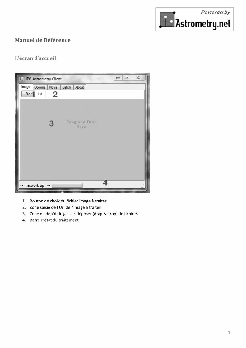
L’écran d’accueil
1. Bouton de choix du fichier image à traiter 2. Zone saisie de l’Url de l’image à traiter 3. Zone de dépôt du glisser-déposer (drag & drop) de fichiers 4. Barre d’état du traitement
5
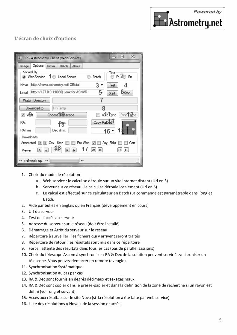
L’écran de choix d’options
1. Choix du mode de résolution a. Web service : le calcul se déroule sur un site internet distant (Url en 3) b. Serveur sur ce réseau : le calcul se déroule localement (Url en 5) c. Le calcul est effectué sur ce calculateur en Batch (La commande est paramétrable dans l’onglet
Batch. 2. Aide par bulles en anglais ou en Français (développement en cours) 3. Url du serveur 4. Test de l’accès au serveur 5. Adresse du serveur sur le réseau (doit être installé) 6. Démarrage et Arrêt du serveur sur le réseau 7. Répertoire à surveiller : les fichiers qui y arrivent seront traités 8. Répertoire de retour : les résultats sont mis dans ce répertoire 9. Force l’attente des résultats dans tous les cas (pas de parallélisassions) 10. Choix du télescope Ascom à synchroniser : RA & Dec de la solution peuvent servir à synchroniser un
télescope. Vous pouvez démarrer en remote (aveugle). 11. Synchronisation Systématique 12. Synchronisation au cas par cas 13. RA & Dec sont fournis en degrés décimaux et sexagésimaux 14. RA & Dec sont copier dans le presse-papier et dans la définition de la zone de recherche si un rayon est
défini (voir onglet suivant) 15. Accès aux résultats sur le site Nova (si la résolution a été faite par web service) 16. Liste des résolutions « Nova » de la session et accès.
6
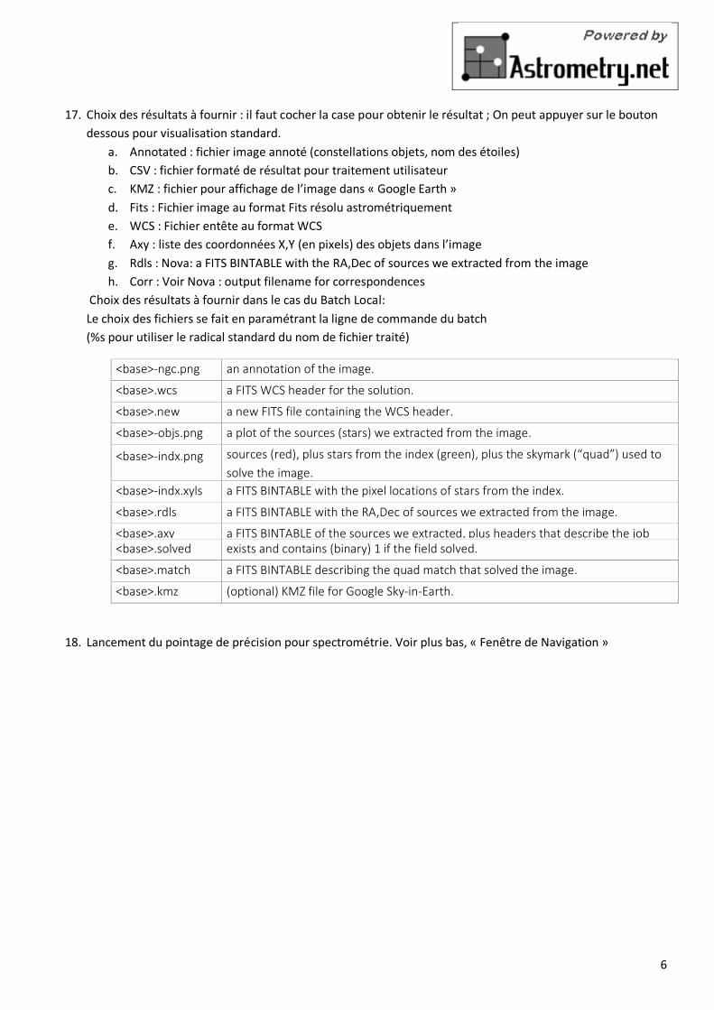
17. Choix des résultats à fournir : il faut cocher la case pour obtenir le résultat ; On peut appuyer sur le bouton dessous pour visualisation standard.
a. Annotated : fichier image annoté (constellations objets, nom des étoiles) b. CSV : fichier formaté de résultat pour traitement utilisateur c. KMZ : fichier pour affichage de l’image dans « Google Earth » d. Fits : Fichier image au format Fits résolu astrométriquement e. WCS : Fichier entête au format WCS f. Axy : liste des coordonnées X,Y (en pixels) des objets dans l’image g. Rdls : Nova: a FITS BINTABLE with the RA,Dec of sources we extracted from the image h. Corr : Voir Nova : output filename for correspondences
Choix des résultats à fournir dans le cas du Batch Local: Le choix des fichiers se fait en paramétrant la ligne de commande du batch (%s pour utiliser le radical standard du nom de fichier traité)
<base>-ngc.png an annotation of the image. <base>.wcs a FITS WCS header for the solution. <base>.new a new FITS file containing the WCS header. <base>-objs.png a plot of the sources (stars) we extracted from the image.
<base>-indx.png sources (red), plus stars from the index (green), plus the skymark (“quad”) used to solve the image.
<base>-indx.xyls a FITS BINTABLE with the pixel locations of stars from the index. <base>.rdls a FITS BINTABLE with the RA,Dec of sources we extracted from the image. <base>.axy a FITS BINTABLE of the sources we extracted, plus headers that describe the job <base>.solved exists and contains (binary) 1 if the field solved. <base>.match a FITS BINTABLE describing the quad match that solved the image. <base>.kmz (optional) KMZ file for Google Sky-in-Earth.
18. Lancement du pointage de précision pour spectrométrie. Voir plus bas, « Fenêtre de Navigation »
7
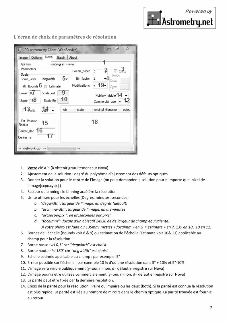
L’écran de choix de paramètres de résolution
1. Votre clé API (à obtenir gratuitement sur Nova) 2. Ajustement de la solution : degré du polynôme d’ajustement des défauts optiques. 3. Donner la solution pour le centre de l’image (on peut demander la solution pour n’importe quel pixel de
l’image[cxpx,cypx] ) 4. Facteur de binning : le binning accélère la résolution. 5. Unité utilisée pour les échelles (Degrés, minutes, secondes)
a. "degwidth": largeur de l’image, en degrés (default) b. "arcminwidth": largeur de l’image, en arcminutes c. "arcsecperpix ": en arcsecondes par pixel d. "focalmm": focale d’un objectif 24x36 de de largeur de champ équivalente.
si votre photo est faite au 135mm, mettez « focalmm » en 6, « estimate » en 7, 135 en 10 , 10 en 11. 6. Bornes de l’échelle (Bounds voir 8 & 9) ou estimation de l’échelle (Estimate voir 10& 11) applicable au
champ pour la résolution. 7. Borne basse : Ici 0,1° car "degwidth" est choisi. 8. Borne haute : Ici 180° car "degwidth" est choisi. 9. Echelle estimée applicable au champ : par exemple 5° 10. Erreur possible sur l’échelle : par exemple 10 % d’où une résolution dans 5° + 10% et 5°-10% 11. L’image sera visible publiquement (y=oui, n=non, d= défaut enregistré sur Nova) 12. L’image pourra être utilisée commercialement (y=oui, n=non, d= défaut enregistré sur Nova) 13. La parité peut être fixée par la dernière résolution. 14. Choix de la parité pour la résolution : Paire ou impaire ou les deux (both). Si la parité est connue la résolution
est plus rapide. La parité est liée au nombre de miroirs dans le chemin optique. La parité trouvée est fournie au retour.
8
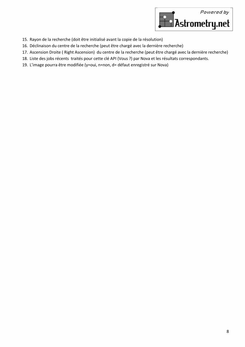
15. Rayon de la recherche (doit être initialisé avant la copie de la résolution) 16. Déclinaison du centre de la recherche (peut être chargé avec la dernière recherche) 17. Ascension Droite ( Right Ascension) du centre de la recherche (peut être chargé avec la dernière recherche) 18. Liste des jobs récents traités pour cette clé API (Vous ?) par Nova et les résultats correspondants. 19. L’image pourra être modifiée (y=oui, n=non, d= défaut enregistré sur Nova)
9
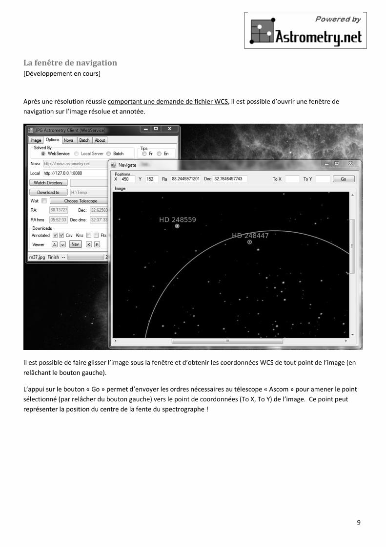
La fenêtre de navigation [Développement en cours]
Après une résolution réussie comportant une demande de fichier WCS, il est possible d’ouvrir une fenêtre de navigation sur l’image résolue et annotée.
Il est possible de faire glisser l’image sous la fenêtre et d’obtenir les coordonnées WCS de tout point de l’image (en relâchant le bouton gauche).
L’appui sur le bouton « Go » permet d’envoyer les ordres nécessaires au télescope « Ascom » pour amener le point sélectionné (par relâcher du bouton gauche) vers le point de coordonnées (To X, To Y) de l’image. Ce point peut représenter la position du centre de la fente du spectrographe !
10
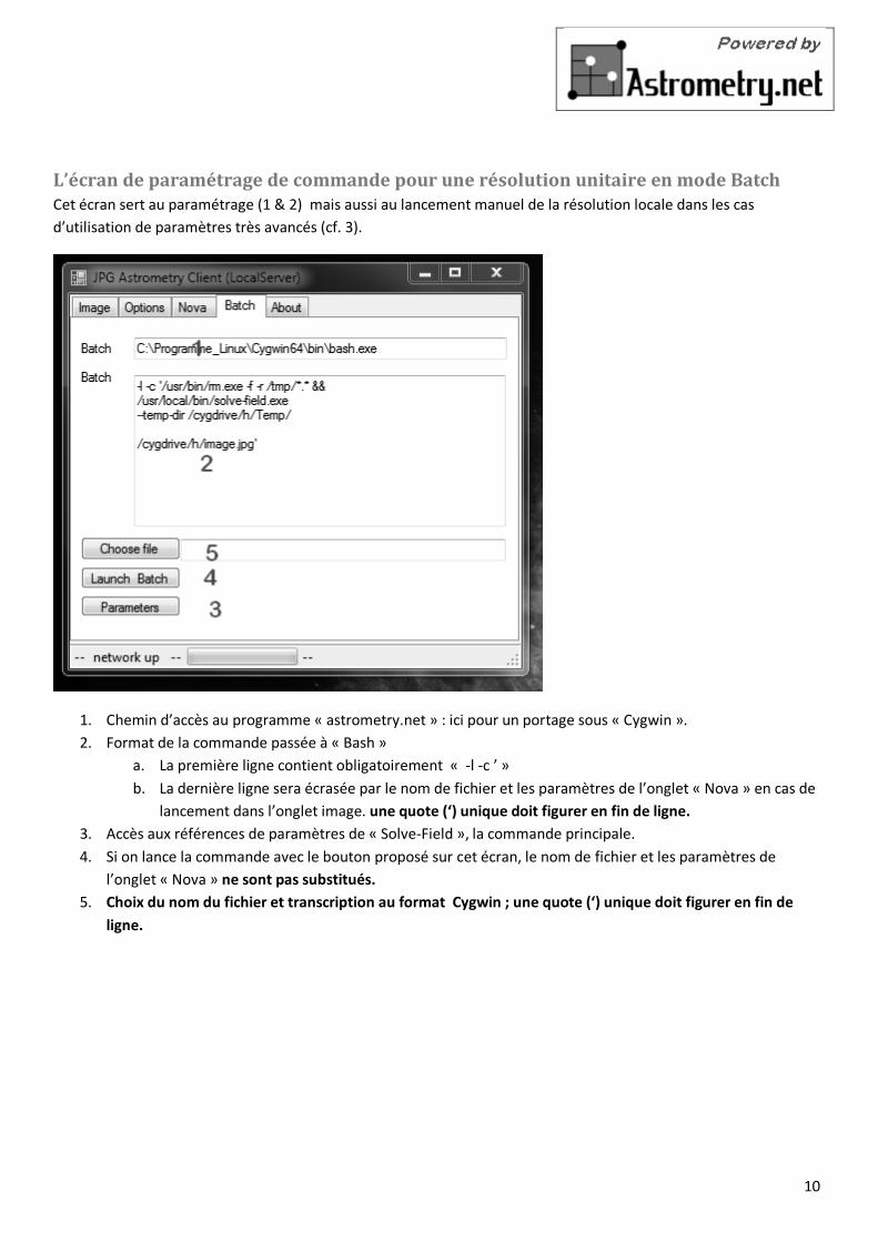
L’écran de paramétrage de commande pour une résolution unitaire en mode Batch Cet écran sert au paramétrage (1 & 2) mais aussi au lancement manuel de la résolution locale dans les cas d’utilisation de paramètres très avancés (cf. 3).
1. Chemin d’accès au programme « astrometry.net » : ici pour un portage sous « Cygwin ». 2. Format de la commande passée à « Bash »
a. La première ligne contient obligatoirement « -l -c ’ » b. La dernière ligne sera écrasée par le nom de fichier et les paramètres de l’onglet « Nova » en cas de
lancement dans l’onglet image. une quote (‘) unique doit figurer en fin de ligne. 3. Accès aux références de paramètres de « Solve-Field », la commande principale. 4. Si on lance la commande avec le bouton proposé sur cet écran, le nom de fichier et les paramètres de
l’onglet « Nova » ne sont pas substitués. 5. Choix du nom du fichier et transcription au format Cygwin ; une quote (‘) unique doit figurer en fin de
ligne.
11
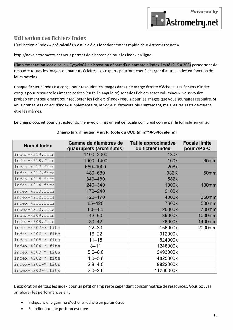
Utilisation des fichiers Index L’utilisation d’index « pré calculés » est la clé du fonctionnement rapide de « Astrometry.net ».
http://nova.astrometry.net vous permet de disposer de tous les index en ligne.
L’implémentation locale sous « Cygwin64 » dispose au départ d’un nombre d’index limité (219 à 208) permettant de résoudre toutes les images d’amateurs éclairés. Les experts pourront cher à charger d’autres index en fonction de leurs besoins.
Chaque fichier d'index est conçu pour résoudre les images dans une marge étroite d'échelle. Les fichiers d'index conçus pour résoudre les images petites (en taille angulaire) sont des fichiers assez volumineux, vous voulez probablement seulement pour récupérer les fichiers d'index requis pour les images que vous souhaitez résoudre. Si vous prenez les fichiers d'index supplémentaire, le Solveur s'exécute plus lentement, mais les résultats devraient être les mêmes.
Le champ couvert pour un capteur donné avec un instrument de focale connu est donné par la formule suivante:
Champ (arc minutes) = arctg[(côté du CCD (mm)*10-3)/focale(m)]
Nom d’Index Gamme de diamètres de quadruplets (arcminutes)
Taille approximative du fichier index
Focale limite pour APS-C
index-4219.fits 1400–2000 130k index-4218.fits 1000–1400 160k 35mm index-4217.fits 680–1000 208k index-4216.fits 480–680 332K 50mm index-4215.fits 340–480 582k index-4214.fits 240–340 1000k 100mm index-4213.fits 170–240 2100k index-4212.fits 120–170 4000k 350mm index-4211.fits 85–120 7600k 500mm index-4210.fits 60—85 20000k 700mm index-4209.fits 42–60 39000k 1000mm index-4208.fits 30–42 78000k 1400mm index-4207-*.fits 22–30 156000k 2000mm index-4206-*.fits 16–22 312000k index-4205-*.fits 11–16 624000k index-4204-*.fits 8–11 1248000k index-4203-*.fits 5.6–8.0 2493000k index-4202-*.fits 4.0–5.6 4825000k index-4201-*.fits 2.8–4.0 8822000k index-4200-*.fits 2.0–2.8 11280000k
L’exploration de tous les index pour un petit champ reste cependant consommatrice de ressources. Vous pouvez améliorer les performances en :
• Indiquant une gamme d’échelle réaliste en paramètres • En indiquant une position estimée
12
• En supprimant les index non utilisés [Solveur Local] (ciel austral, champ non couvert,…)
Traitement des images couleurs
Le traitement utilise "ppmtopgm", http://netpbm.sourceforge.net/doc/ppmtopgm.html donc une somme pondérée des canaux R,G,B. Il n'y a pas d'option pour sélectionner le canal. Vous devez ré-enregistrer en niveaux de gris pour obtenir un comportement différent.
13
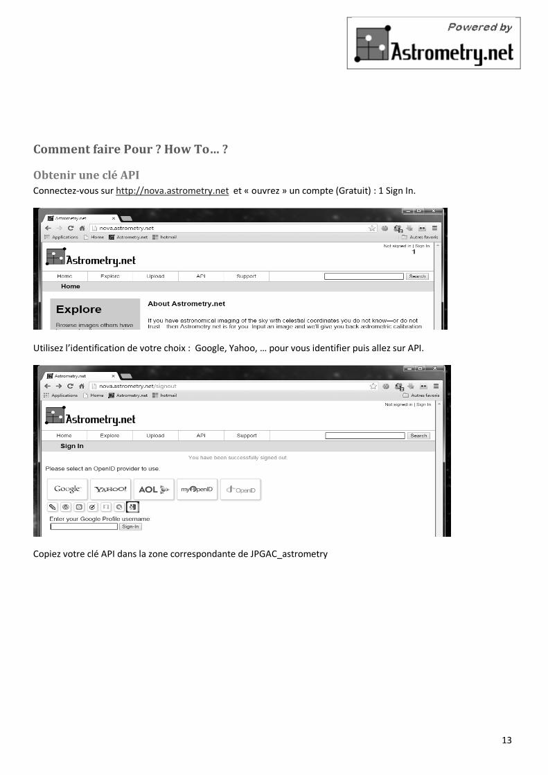
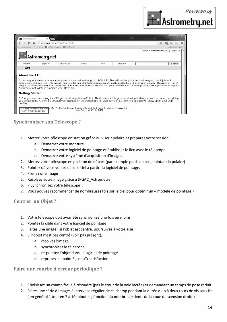
Comment faire Pour ? How To… ?
Obtenir une clé API Connectez-vous sur http://nova.astrometry.net et « ouvrez » un compte (Gratuit) : 1 Sign In.
Utilisez l’identification de votre choix : Google, Yahoo, … pour vous identifier puis allez sur API.
Copiez votre clé API dans la zone correspondante de JPGAC_astrometry
14
Synchroniser son Télescope ?
1. Mettez votre télescope en station grâce au viseur polaire et préparez votre session a. Démarrez votre monture b. Démarrez votre logiciel de pointage et établissez le lien avec le télescope c. Démarrez votre système d’acquisition d’images
2. Mettez votre télescope en position de départ (par exemple poids en bas, pointant la polaire) 3. Pointez où vous voulez dans le ciel à partir du logiciel de pointage. 4. Prenez une image 5. Résolvez votre image grâce à JPGAC_Astrometry 6. « Synchronisez votre télescope » 7. Vous pouvez recommencer de nombreuses fois sur le ciel pour obtenir un « modèle de pointage »
Centrer un Objet ?
1. Votre télescope doit avoir été synchronisé une fois au moins… 2. Pointez la cible dans votre logiciel de pointage 3. Faites une image : si l’objet est centré, poursuivez à votre aise 4. Si l’objet n’est pas centré (voir pas présent),
a. résolvez l’image b. synchronisez le télescope c. re-pointez l’objet dans le logiciel de pointage d. reprenez au point 3 jusqu’à satisfaction.
Faire une courbe d’erreur périodique ?
1. Choisissez un champ facile à résoudre (pas le cœur de la voie lactée) et demandant un temps de pose réduit 2. Faites une série d’images à intervalle régulier de ce champ pendant la durée d’un à deux tours de vis sans fin
( en général 1 tour en 7 à 10 minutes ; fonction du nombre de dents de la roue d’ascension droite)

15
3. Résolvez toutes les images (avec option CSV) 4. Utilisez les fichiers CSV avec un tableur pour faire un Tableau de RA et Dec en fonction du temps. (Le fichier
log général reprend toutes les résolutions)
Faire une image pour « Google Earth » ?
1. Résolvez une image en demandant le fichier « KMZ » 2. Double cliquez sur le fichier pour le lancer dans « Google Earth »
16
Références
http://nova.astrometry.net/ le site en ligne de résolution.
http://astrometry.net/ Le site du Projet « Astrometry.net »
http://astrometry.net/doc/readme.html La documentation US
https://www.flickr.com/groups/astrometry Le groupe Flickr
http://arxiv.org/abs/0910.2233 La publication de référence
Licences
The Astrometry.net code suite is free software licensed under the GNU GPL, version 2. See the file LICENSE for the full terms of the GNU GPL.
The index files come with their own license conditions. See the file GETTING-INDEXES for details.
Copyright 2006-2010 Michael Blanton, David W. Hogg, Dustin Lang, Keir Mierle and Sam Roweis.
Copyright 2011-2013 Dustin Lang and David W. Hogg.
This code is accompanied by the paper:
Lang, D., Hogg, D. W.; Mierle, K., Blanton, M., & Roweis, S., 2010, Astrometry.net: Blind astrometric calibration of arbitrary astronomical images, Astronomical Journal 137, 1782–1800. http://arxiv.org/abs/0910.2233
The original purpose of this code release was to back up the claims in the paper in the interest of scientific repeatability. Over the years, it has become more robust and usable for a wider audience, but it’s still neither totally easy nor bug-free.
JPGAC_Astrometry inclut tout ou parties des logiciels suivants
Astrometry.net © D.Lang, D.W. Hogg
Copyright 2006-2010 Michael Blanton, David W. Hogg, Dustin Lang, Keir Mierle and Sam Roweis. Copyright 2011-2013 Dustin Lang and David W. Hogg.
FitsPng © F. Hroch © JP. Godard pour portage Win64 Bifconv © R. Behrend Dcraw © D. Coffin Wcs2kml © J. Brewer © JP. Godard pour adaptation libpng15
JPGAC_Astrometry est un « Freeware ». L’usage privé est libre.
17
Complément de documentation Astrometry.net en anglais.
Astrometry.net code README
Copyright 2006-2010 Michael Blanton, David W. Hogg, Dustin Lang, Keir Mierle and Sam Roweis.
Copyright 2011-2013 Dustin Lang and David W. Hogg.
This code is accompanied by the paper:
Lang, D., Hogg, D. W.; Mierle, K., Blanton, M., & Roweis, S., 2010, Astrometry.net: Blind astrometric calibration of arbitrary astronomical images, Astronomical Journal 137, 1782–1800. http://arxiv.org/abs/0910.2233
The original purpose of this code release was to back up the claims in the paper in the interest of scientific repeatability. Over the years, it has become more robust and usable for a wider audience, but it’s still neither totally easy nor bug-free.
This release includes a snapshot of all of the components of our current research code, including routines to:
• Convert raw USNO-B and Tycho2 into FITS format for easier use • Uniformize, deduplicate, and cut the FITSified catalogs • Build index files from these cuts • Solve the astrometry of images using these index files
The code includes:
• A simple but powerful HEALPIX implementation • The QFITS library with several modifications • libkd, a compact and high-performance kdtree library
The code requires index files, processed from an astrometric reference catalog such as USNO-B1 or 2MASS. We have released several of these; see Getting Index Files.
Installing
See Building/installing the Astrometry.net code.
Getting Index Files
Get pre-cooked index files from: <http://data.astrometry.net/4200>_ (these are built from the 2MASS catalog).
18
Or, for wide-angle images, <http://data.astrometry.net/4100>_ (these are built from the Tycho-2 catalog).
We used to have the “4000-series” files, but these suffer from a bug where parts of the sky do are not covered by the reference catalog.
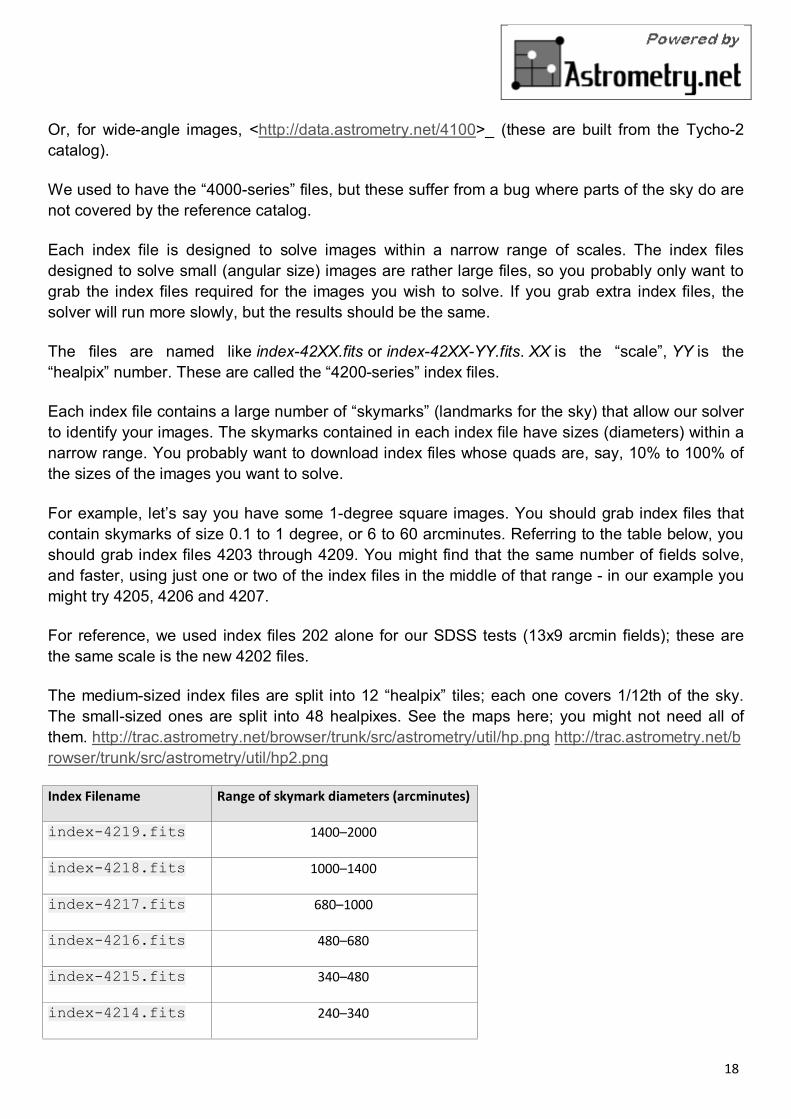
Each index file is designed to solve images within a narrow range of scales. The index files designed to solve small (angular size) images are rather large files, so you probably only want to grab the index files required for the images you wish to solve. If you grab extra index files, the solver will run more slowly, but the results should be the same.
The files are named like index-42XX.fits or index-42XX-YY.fits. XX is the “scale”, YY is the “healpix” number. These are called the “4200-series” index files.
Each index file contains a large number of “skymarks” (landmarks for the sky) that allow our solver to identify your images. The skymarks contained in each index file have sizes (diameters) within a narrow range. You probably want to download index files whose quads are, say, 10% to 100% of the sizes of the images you want to solve.
For example, let’s say you have some 1-degree square images. You should grab index files that contain skymarks of size 0.1 to 1 degree, or 6 to 60 arcminutes. Referring to the table below, you should grab index files 4203 through 4209. You might find that the same number of fields solve, and faster, using just one or two of the index files in the middle of that range - in our example you might try 4205, 4206 and 4207.
For reference, we used index files 202 alone for our SDSS tests (13x9 arcmin fields); these are the same scale is the new 4202 files.
The medium-sized index files are split into 12 “healpix” tiles; each one covers 1/12th of the sky. The small-sized ones are split into 48 healpixes. See the maps here; you might not need all of them. http://trac.astrometry.net/browser/trunk/src/astrometry/util/hp.png http://trac.astrometry.net/browser/trunk/src/astrometry/util/hp2.png
Index Filename Range of skymark diameters (arcminutes)
index-4219.fits 1400–2000
index-4218.fits 1000–1400
index-4217.fits 680–1000
index-4216.fits 480–680
index-4215.fits 340–480
index-4214.fits 240–340
19
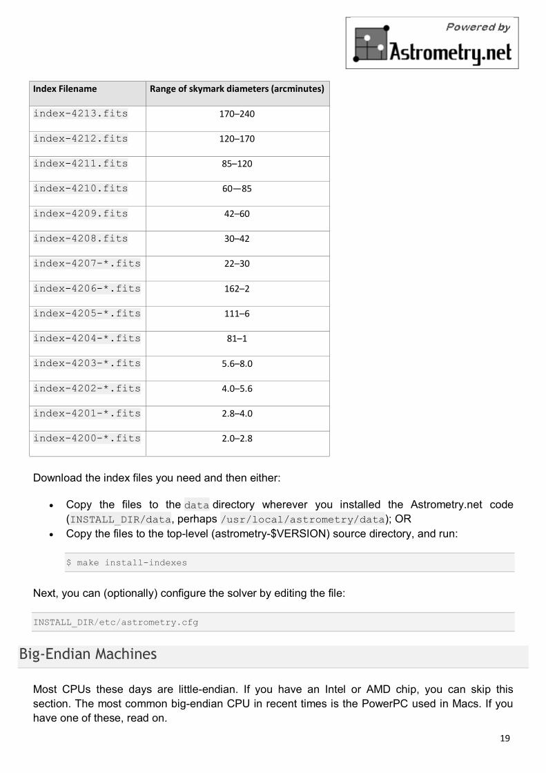
Index Filename Range of skymark diameters (arcminutes)
index-4213.fits 170–240
index-4212.fits 120–170
index-4211.fits 85–120
index-4210.fits 60—85
index-4209.fits 42–60
index-4208.fits 30–42
index-4207-*.fits 22–30
index-4206-*.fits 162–2
index-4205-*.fits 111–6
index-4204-*.fits 81–1
index-4203-*.fits 5.6–8.0
index-4202-*.fits 4.0–5.6
index-4201-*.fits 2.8–4.0
index-4200-*.fits 2.0–2.8
Download the index files you need and then either:
• Copy the files to the data directory wherever you installed the Astrometry.net code (INSTALL_DIR/data, perhaps /usr/local/astrometry/data); OR
• Copy the files to the top-level (astrometry-$VERSION) source directory, and run:
$ make install-indexes
Next, you can (optionally) configure the solver by editing the file:
INSTALL_DIR/etc/astrometry.cfg
Big-Endian Machines
Most CPUs these days are little-endian. If you have an Intel or AMD chip, you can skip this section. The most common big-endian CPU in recent times is the PowerPC used in Macs. If you have one of these, read on.
20
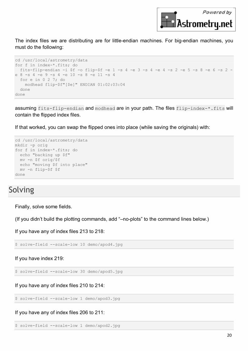
The index files we are distributing are for little-endian machines. For big-endian machines, you must do the following:
cd /usr/local/astrometry/data for f in index-*.fits; do fits-flip-endian -i $f -o flip-$f -e 1 -s 4 -e 3 -s 4 -e 4 -s 2 -e 5 -s 8 -e 6 -s 2 -e 8 -s 4 -e 9 -s 4 -e 10 -s 8 -e 11 -s 4 for e in 0 2 7; do modhead flip-$f"[$e]" ENDIAN 01:02:03:04 done done
assuming fits-flip-endian and modhead are in your path. The files flip-index-*.fits will contain the flipped index files.
If that worked, you can swap the flipped ones into place (while saving the originals) with:
cd /usr/local/astrometry/data mkdir -p orig for f in index-*.fits; do echo "backing up $f" mv -n $f orig/$f echo "moving $f into place" mv -n flip-$f $f done
Solving
Finally, solve some fields.
(If you didn’t build the plotting commands, add “–no-plots” to the command lines below.)
If you have any of index files 213 to 218:
$ solve-field --scale-low 10 demo/apod4.jpg
If you have index 219:
$ solve-field --scale-low 30 demo/apod5.jpg
If you have any of index files 210 to 214:
$ solve-field --scale-low 1 demo/apod3.jpg
If you have any of index files 206 to 211:
$ solve-field --scale-low 1 demo/apod2.jpg
21
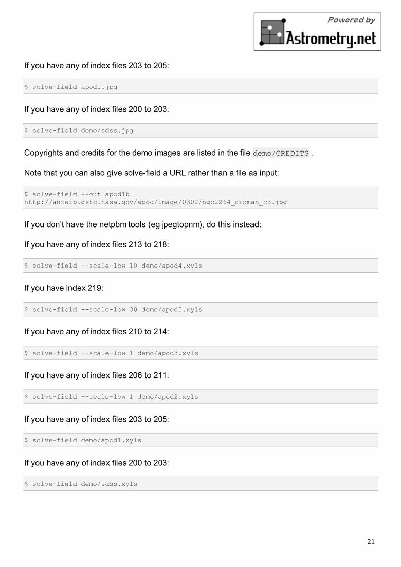
If you have any of index files 203 to 205:
$ solve-field apod1.jpg
If you have any of index files 200 to 203:
$ solve-field demo/sdss.jpg
Copyrights and credits for the demo images are listed in the file demo/CREDITS .
Note that you can also give solve-field a URL rather than a file as input:
$ solve-field --out apod1b http://antwrp.gsfc.nasa.gov/apod/image/0302/ngc2264_croman_c3.jpg
If you don’t have the netpbm tools (eg jpegtopnm), do this instead:
If you have any of index files 213 to 218:
$ solve-field --scale-low 10 demo/apod4.xyls
If you have index 219:
$ solve-field --scale-low 30 demo/apod5.xyls
If you have any of index files 210 to 214:
$ solve-field --scale-low 1 demo/apod3.xyls
If you have any of index files 206 to 211:
$ solve-field --scale-low 1 demo/apod2.xyls
If you have any of index files 203 to 205:
$ solve-field demo/apod1.xyls
If you have any of index files 200 to 203:
$ solve-field demo/sdss.xyls
22
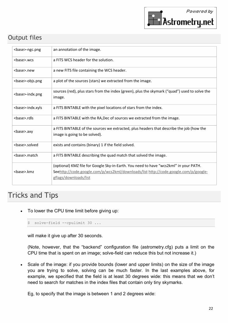
Output files
<base>-ngc.png an annotation of the image.
<base>.wcs a FITS WCS header for the solution.
<base>.new a new FITS file containing the WCS header.
<base>-objs.png a plot of the sources (stars) we extracted from the image.
<base>-indx.png sources (red), plus stars from the index (green), plus the skymark (“quad”) used to solve the image.
<base>-indx.xyls a FITS BINTABLE with the pixel locations of stars from the index.
<base>.rdls a FITS BINTABLE with the RA,Dec of sources we extracted from the image.
<base>.axy a FITS BINTABLE of the sources we extracted, plus headers that describe the job (how the image is going to be solved).
<base>.solved exists and contains (binary) 1 if the field solved.
<base>.match a FITS BINTABLE describing the quad match that solved the image.
<base>.kmz (optional) KMZ file for Google Sky-in-Earth. You need to have “wcs2kml” in your PATH. Seehttp://code.google.com/p/wcs2kml/downloads/list http://code.google.com/p/google-gflags/downloads/list
Tricks and Tips
• To lower the CPU time limit before giving up:
$ solve-field --cpulimit 30 ...
will make it give up after 30 seconds.
(Note, however, that the “backend” configuration file (astrometry.cfg) puts a limit on the CPU time that is spent on an image; solve-field can reduce this but not increase it.)
• Scale of the image: if you provide bounds (lower and upper limits) on the size of the image you are trying to solve, solving can be much faster. In the last examples above, for example, we specified that the field is at least 30 degrees wide: this means that we don’t need to search for matches in the index files that contain only tiny skymarks.
Eg, to specify that the image is between 1 and 2 degrees wide:
23
$ solve-field --scale-units degwidth --scale-low 1 --scale-high 2 ...
If you know the pixel scale instead:
$ solve-field --scale-units arcsecperpix \ --scale-low 0.386 --scale-high 0.406 ...
When you tell solve-field the scale of your image, it uses this to decide which index files to try to use to solve your image; each index file contains quads whose scale is within a certain range, so if these quads are too big or too small to be in your image, there is no need to look in that index file. It is also used while matching quads: a small quad in your image is not allowed to match a large quad in the index file if such a match would cause the image scale to be outside the bounds you specified. However, all these checks are done before computing a best-fit WCS solution and polynomial distortion terms, so it is possible (though rare) for the final solution to fall outside the limits you specified. This should only happen when the solution is correct, but you gave incorrect inputs, so you shouldn’t be complaining! :)
• Guess the scale: solve-field can try to guess your image’s scale from a number of different FITS header values. When it’s right, this often speeds up solving a lot, and when it’s wrong it doesn’t cost much. Enable this with:
$ solve-field --guess-scale ...
• If you’ve got big images: you might want to downsample them before doing source extraction:
• $ solve-field --downsample 2 ...
$ solve-field --downsample 4 ...
• Depth. The solver works by looking at sources in your image, starting with the brightest. It searches for all “skymarks” that can be built from the N brightest stars before considering star N+1. When using several index files, it can be much faster to search for many skymarks in one index file before switching to the next one. This flag lets you control when the solver switches between index files. It also lets you control how much effort the solver puts in before giving up - by default it looks at all the sources in your image, and usually times out before this finishes.
Eg, to first look at sources 1-20 in all index files, then sources 21-30 in all index files, then 31-40:
$ solve-field --depth 20,30,40 ...
or:
24
$ solve-field --depth 1-20 --depth 21-30 --depth 31-40 ...
Sources are numbered starting at one, and ranges are inclusive. If you don’t give a lower limit, it will take 1 + the previous upper limit. To look at a single source, do:
$ solve-field --depth 42-42 ...
• Our source extractor sometimes estimates the background badly, so by default we sort the stars by brightness using a compromise between the raw and background-subtracted flux estimates. For images without much nebulosity, you might find that using the background-subtracted fluxes yields faster results. Enable this by:
$ solve-field --resort ...
• If you’ve got big images: you might want to downsample them before doing source extraction:
$ solve-field --downsample 2 ...
or:
$ solve-field --downsample 4 ...
• When solve-field processes FITS files, it runs them through a “sanitizer” which tries to clean up non-standards-compliant images. If your FITS files are compliant, this is a waste of time, and you can avoid doing it:
$ solve-field --no-fits2fits ...
• When solve-field processes FITS images, it looks for an existing WCS header. If one is found, it tries to verify that header before trying to solve the image blindly. You can prevent this with:
$ solve-field --no-verify ...
Note that currently solve-field only understands a small subset of valid WCS headers: essentially just the TAN projection with a CD matrix (not CROT).
• If you don’t want the plots to be produced:
$ solve-field --no-plots ...
• “I know where my image is to within 1 arcminute, how can I tell solve-field to only look there?”
25
$ solve-field --ra, --dec, --radius
Tells it to look within “radius” degrees of the given RA,Dec position.
• To convert a list of pixel coordinates to RA,Dec coordinates:
$ wcs-xy2rd -w wcs-file -i xy-list -o radec-list
Where xy-list is a FITS BINTABLE of the pixel locations of sources; recall that FITS specifies that the center of the first pixel is pixel coordinate (1,1).
• To convert from RA,Dec to pixels:
$ wcs-rd2xy -w wcs-file -i radec-list -o xy-list
• To make cool overlay plots: see plotxy, plot-constellations. • To change the output filenames when processing multiple input files: each of the output
filename options listed below can include “%s”, which will be replaced by the base output filename. (Eg, the default for –wcs is “%s.wcs”). If you really want a “%” character in your output filename, you have to put “%%”.
Outputs include:
o –new-fits o –kmz o –solved o –cancel o –match o –rdls o –corr o –wcs o –keep-xylist o –pnm
also included:
o –solved-in o –verify
• Reusing files between runs:
The first time you run solve-field, save the source extraction results:
$ solve-field --keep-xylist %s.xy input.fits ...
26
On subsequent runs, instead of using the original input file, use the saved xylist instead. Also add --continue to overwrite any output file that already exists.
$ solve-field input.xy --no-fits2fits --continue ...
To skip previously solved inputs (note that this assumes single-HDU inputs):
$ solve-field --skip-solved ...
Optimizing the code
Here are some things you can do to make the code run faster:
• we try to guess “-mtune” settings that will work for you; if we’re wrong, you can set the environment variable ARCH_FLAGS before compiling:
$ ARCH_FLAGS=”-mtune=nocona” make
You can find details in the gcc manual:
http://gcc.gnu.org/onlinedocs/
You probably want to look in the section:
“GCC Command Options”
-> “Hardware Models and Configurations”
-> “Intel 386 and AMD x86-64 Options”
http://gcc.gnu.org/onlinedocs/gcc-4.3.0/gcc/i386-and-x86_002d64-Options.html#i386-and-x86_002d64-Options
What are all these programs?
When you “make install”, you’ll get a bunch of programs in /usr/local/astrometry/bin. Here’s a brief synopsis of what each one does. For more details, run the program without arguments (most of them give at least a brief summary of what they do).
Image-solving programs:
• solve-field: main high-level command-line user interface. • backend: higher-level solver that reads “augmented xylists”; called by solve-field. • augment-xylist: creates “augmented xylists” from images, which include star positions and hints and
instructions for solving.
27
• blind: low-level command-line solver. • image2xy: source extractor.
Plotting programs:
• plotxy: plots circles, crosses, etc over images. • plotquad: draws polygons over images. • plot-constellations: annotates images with constellations, bright stars, Messier/NGC objects, Henry
Draper catalog stars, etc. • plotcat: produces density plots given lists of stars.
WCS utilities:
• new-wcs: merge a WCS solution with existing FITS header cards; can be used to create a new image file containing the WCS headers.
• fits-guess-scale: try to guess the scale of an image based on FITS headers. • wcsinfo: print simple properties of WCS headers (scale, rotation, etc) • wcs-xy2rd, wcs-rd2xy: convert between lists of pixel (x,y) and (RA,Dec) positions. • wcs-resample: projects one FITS image onto another image. • wcs-grab/get-wcs: try to interpret an existing WCS header.
Miscellany:
• an-fitstopnm: converts FITS images into ugly PNM images. • get-healpix: which healpix covers a given RA,Dec? • hpowned: which small healpixels are inside a big healpixel? • control-program: sample code for how you might use the Astrometry.net code in your own software. • xylist2fits: converts a text list of x,y positions to a FITS binary table. • rdlsinfo: print stats about a list of RA,Dec positions (rdlist). • xylsinfo: print stats about a list of x,y positions (xylist).
FITS utilities
• tablist: list values in a FITS binary table. • modhead: print or modify FITS header cards. • fitscopy: general FITS image / table copier. • tabmerge: combines rows in two FITS tables. • fitstomatlab: prints out FITS binary tables in a silly format. • liststruc: shows the structure of a FITS file. • listhead: prints FITS header cards. • imcopy: copies FITS images. • imarith: does (very) simple arithmetic on FITS images. • imstat: computes statistics on FITS images. • fitsgetext: pull out individual header or data blocks from multi-HDU FITS files.
28
• subtable: pull out a set of columns from a many-column FITS binary table. • tabsort: sort a FITS binary table based on values in one column. • column-merge: create a FITS binary table that includes columns from two input tables. • add-healpix-column: given a FITS binary table containing RA and DEC columns, compute the
HEALPIX and add it as a column. • resort-xylist: used by solve-field to sort a list of stars using a compromise between background-
subtracted and non-background-subtracted flux (because our source extractor sometimes messes up the background subtraction).
• fits-flip-endian: does endian-swapping of FITS binary tables. • fits-dedup: removes duplicate header cards.
Index-building programs
• build-index: given a FITS binary table with RA,Dec, build an index file. This is the “easy”, recent way. The old way uses the rest of these programs:
o usnobtofits, tycho2tofits, nomadtofits, 2masstofits: convert catalogs into FITS binary tables. o build-an-catalog: convert input catalogs into a standard FITS binary table format. o cut-an: grab a bright, uniform subset of stars from a catalog. o startree: build a star kdtree from a catalog. o hpquads: find a bright, uniform set of N-star features. o codetree: build a kdtree from N-star shape descriptors. o unpermute-quads, unpermute-stars: reorder index files for efficiency.
• hpsplit: splits a list of FITS tables into healpix tiles
Source lists (“xylists”)
The solve-field program accepts either images or “xylists” (xyls), which are just FITS BINTABLE files which contain two columns (float or double (E or D) format) which list the pixel coordinates of sources (stars, etc) in the image.
To specify the column names (eg, “XIMAGE” and “YIMAGE”):
$ solve-field --x-column XIMAGE --y-column YIMAGE ...
Our solver assumes that the sources are listed in order of brightness, with the brightest sources first. If your files aren’t sorted, you can specify a column by which the file should be sorted.
$ solve-field --sort-column FLUX ...
By default it sorts with the largest value first (so it works correctly if the column contains FLUX values), but you can reverse that by:
$ solve-field --sort-ascending --sort-column MAG ...
29
When using xylists, you should also specify the original width and height of the image, in pixels:
$ solve-field --width 2000 --height 1500 ...
Alternatively, if the FITS header contains “IMAGEW” and “IMAGEH” keys, these will be used.
The solver can deal with multi-extension xylists; indeed, this is a convenient way to solve a large number of fields at once. You can tell it which extensions it should solve by:
$ solve-field --fields 1-100,120,130-200
(Ranges of fields are inclusive, and the first FITS extension is 1, as per the FITS standard.)
Unfortunately, the plotting code isn’t smart about handling multiple fields, so if you’re using multi-extension xylists you probably want to turn off plotting:
$ solve-field --no-plots ...
Backend config
Because we also operate a web service using most of the same software, the local version of the solver is a bit more complicated than it really needs to be. The “solve-field” program takes your input files, does source extraction on them to produce an “xylist” – a FITS BINTABLE of source positions – then takes the information you supplied about your fields on the command-line and adds FITS headers encoding this information. We call this file an “augmented xylist”; we use the filename suffix ”.axy”. “solve-field” then calls the “backend” program, passing it your axy file. “backend” reads a config file (by default /usr/local/astrometry/etc/astrometry.cfg) that describes things like where to find index files, whether to load all the index files at once or run them one at a time, how long to spend on each field, and so on. If you want to force only a certain set of index files to load, you can copy the astrometry.cfg file to a local version and change the list of index files that are loaded, and then tell solve-field to use this config file:
$ solve-field --config myastrometry.cfg ...
SExtractor
http://www.astromatic.net/software/sextractor
The “Source Extractor” aka “SExtractor” program by Emmanuel Bertin can be used to do source extraction if you don’t want to use our own bundled “image2xy” program.
NOTE: users have reported that SExtractor 2.4.4 (available in some Ubuntu distributions) DOES NOT WORK – it prints out correct source positions as it runs, but the “xyls” output file it produces
30
contains all (0,0). We haven’t looked into why this is or how to work around it. Later versions of SExtractor such as 2.8.6 work fine.
You can tell solve-field to use SExtractor like this:
$ solve-field --use-sextractor ...
By default we use almost all SExtractor’s default settings. The exceptions are:
1. We write a PARAMETERS_NAME file containing:
X_IMAGE Y_IMAGE MAG_AUTO
2. We write a FILTER_NAME file containing a Gaussian PSF with FWHM of 2 pixels. (See blind/augment-xylist.c “filterstr” for the exact string.)
3. We set CATALOG_TYPE FITS_1.0 4. We set CATALOG_NAME to a temp filename.
If you want to override any of the settings we use, you can use:
$ solve-field --use-sextractor --sextractor-config <sex.conf>
In order to reproduce the default behavior, you must:
1) Create a parameters file like the one we make, and set PARAMETERS_NAME to its filename 2) Set:: $ solve-field --x-column X_IMAGE --y-column Y_IMAGE \ --sort-column MAG_AUTO --sort-ascending 3) Create a filter file like the one we make, and set FILTER_NAME to its filename
Note that you can tell solve-field where to find SExtractor with:
$ solve-field --use-sextractor --sextractor-path <path-to-sex-executable>
Workarounds
• No python
There are two places we use python: handling images, and filtering FITS files.
You can avoid the image-handling code by doing source extraction yourself; see the “No netpbm” section below.
31
You can avoid filtering FITS files by using the “–no-fits2fits” option to solve-field.
• No netpbm
We use the netpbm tools (jpegtopnm, pnmtofits, etc) to convert from all sorts of image formats to PNM and FITS.
If you don’t have these programs installed, you must do source extraction yourself and use “xylists” rather than images as the input to solve-field. See SEXTRACTOR and XYLIST sections above.
ERROR MESSAGES during compiling
1. /bin/sh: line 1: /dev/null: No such file or directory
We’ve seen this happen on Macs a couple of times. Reboot and it goes away...
2. makefile.deps:40: deps: No such file or directory
Not a problem. We use automatic dependency tracking: “make” keeps track of which source files depend on which other source files. These dependencies get stored in a file named “deps”; when it doesn’t exist, “make” tries to rebuild it, but not before printing this message.
3. os-features-test.c: In function 'main': 4. os-features-test.c:23: warning: implicit declaration of function
'canonicalize_file_name' 5. os-features-test.c:23: warning: initialization makes pointer from integer without
a cast 6. /usr/bin/ld: Undefined symbols: 7. _canonicalize_file_name 8. collect2: ld returned 1 exit status
Not a problem. We provide replacements for a couple of OS-specific functions, but we need to decide whether to use them or not. We do that by trying to build a test program and checking whether it works. This failure tells us your OS doesn’t provide the canonicalize_file_name() function, so we plug in a replacement.
9. configure: WARNING: cfitsio: == No acceptable f77 found in $PATH 10. configure: WARNING: cfitsio: == Cfitsio will be built without Fortran wrapper
support 11. drvrfile.c: In function 'file_truncate': 12. drvrfile.c:360: warning: implicit declaration of function 'ftruncate' 13. drvrnet.c: In function 'http_open': 14. drvrnet.c:300: warning: implicit declaration of function 'alarm' 15. drvrnet.c: In function 'http_open_network': 16. drvrnet.c:810: warning: implicit declaration of function 'close' 17. drvrsmem.c: In function 'shared_cleanup': 18. drvrsmem.c:154: warning: implicit declaration of function 'close'
32
19. group.c: In function 'fits_get_cwd': 20. group.c:5439: warning: implicit declaration of function 'getcwd' 21. ar: creating archive libcfitsio.a
Not a problem; these errors come from cfitsio and we just haven’t fixed them.
License
The Astrometry.net code suite is free software licensed under the GNU GPL, version 2. See the file LICENSE for the full terms of the GNU GPL.
The index files come with their own license conditions. See the file GETTING-INDEXES for details.
Contact
You can post questions (or maybe even find the answer to your questions) at http://forum.astrometry.net . However, please also send an email to “code2 at astrometry dot net” pointing out your post to the forum – we never remember to check the forum! We would also be happy to hear via email any bug reports, comments, critiques, feature requests, and in general any reports on your experiences, good or bad.
33
Astrometry.net: Blind astrometric calibration of arbitrary astronomical images
Dustin Lang (1, 2), David W. Hogg (3, 4), Keir Mierle (1, 5), Michael Blanton (3), Sam Roweis (1, 5, 6) ((1) Department of Computer Science, University of Toronto, (2) Princeton University Observatory, (3) Center for Cosmology & Particle Physics, New York University, (4) Max-Planck-Institut für Astronomie, (5) Google Inc., (6) Computer Science Department, New York University)
(Submitted on 12 Oct 2009)
We have built a reliable and robust system that takes as input an astronomical image, and returns as output the pointing, scale, and orientation of that image (the astrometric calibration or WCS information). The system requires no first guess, and works with the information in the image pixels alone; that is, the problem is a generalization of the "lost in space" problem in which nothing--not even the image scale--is known. After robust source detection is performed in the input image, asterisms (sets of four or five stars) are geometrically hashed and compared to pre-indexed hashes to generate hypotheses about the astrometric calibration. A hypothesis is only accepted as true if it passes a Bayesian decision theory test against a background hypothesis. With indices built from the USNO-B Catalog and designed for uniformity of coverage and redundancy, the success rate is 99.9% for contemporary near-ultraviolet and visual imaging survey data, with no false positives. The failure rate is consistent with the incompleteness of the USNO-B Catalog; augmentation with indices built from the 2MASS Catalog brings the completeness to 100% with no false positives. We are using this system to generate consistent and standards-compliant meta-data for digital and digitized imaging from plate repositories, automated observatories, individual scientific investigators, and hobbyists. This is the first step in a program of making it possible to trust calibration meta-data for astronomical data of arbitrary provenance.
Comments: submitted to AJ
Subjects: Instrumentation and Methods for Astrophysics (astro-ph.IM)
Journal reference: Astron J, 139, 1782 (2010)
DOI: 10.1088/0004-6256/139/5/1782
Cite as: arXiv:0910.2233 [astro-ph.IM]
(or arXiv:0910.2233v1 [astro-ph.IM] for this version)
Submission history