JPL D-27015

Mars Science Laboratory (MSL) Focused Technology Program

Camera Calibration and Stereo Vision

Technology Validation Report Revision 1

Prepared By: Document Custodian: Won S. Kim Won S. Kim Robert C. Steinke Robert D. Steele

Adnan I. Ansar Paper copies of this document may not be current and should not be relied on for official purposes. The current version is in the MSL Project Library at http://msl-lib.jpl.nasa.gov/ in the Rover Validation Test Reports folder.

January 2004

Jet Propulsion Laboratory 4800 Oak Grove Drive Pasadena, CA 91109-8099

1

Revision History

Revision Date Description Author Initial

Release 06/09/2003 Initial release Kim, Steinke,

Steele, Ansar Rev. 1 01/28/2004 1. Added validation results of the updated

software after two bug fixes (Section 5) 2. Added comparison of stereo and laser

scanner 3-D data (Section 3.15) 3. Updated stereo range error analysis tables

by using different sets for calibration and evaluation (Tables 5 & 6 in Section 3.14)

Kim, Steinke, Steele, Ansar

Related Documents

Document Name Date Author Technology Functional Design Document: Stereo Vision 06/09/2003 Ansar, Kim

2

Scope The scope of this document is to report the results on test and validation of the JPL camera calibration and stereo vision software algorithms. This algorithm validation process supports technology selection process before flight qualification of the software selected. The test validation matrices for the JPL camera calibration and stereo vision software are shown below. Test Validation Matrix for Camera Calibration Parameters Metrology Targets Calibration

error Camera model X X Laser tracker vs. total station X X Target board accuracy X Volume enclosure of targets X X Number of targets X X Checkerboard vs. dots X X

Test Validation Matrix for Stereo Vision Parameters Disparity

coverage Range error Performance

Correlation window size X X Pyramid level (down sampling) X X Vertical misalignment X X Defocus (image blur) X X Maximum disparity X Stereo baseline X X Stereo localization error X Laser scanner X Ripples X Unsurveyed camera calibration X Comparison with SRI SVS X Stereo vision timing X

3

Acknowledgment This work was carried out at the Jet Propulsion Laboratory, California Institute of Technology, under a contract with the National Aeronautics and Space Administration. We would like to thank many people who helped this work: Larry Matthies and Mark Maimone for reviewing our experimental test plan with good suggestions, Issa Nesnas and Max Bajracharya for providing the CLARAty vision package that supports JPL’s stereo vision and SRI’s SVS, Reg Willson for suggesting the laser tracker technology, Yang Cheng for introducing gator-foam calibration target boards, Jay Wu for designing and fabricating a calibration target stand, Eugene Poyorena and Mark Thompson for laser tracker and total station metrology service, Terry Huntsberger for lending us a total station, Tera Estlin and Dan Gaines for a total station procedure, and Dan Helmick for providing a CAD drawing of the stereo camera head face plate.

4

Contents Signature Sheet……………………………………….………………….………………….… 1 Revision History…………………………………………………………………………….… 2 Related Documents………………………………………………………………………...…. 2 Scope……………………………………………………………………………………..……. 3 Acknowledgment……………………………………………………………………… 4 Summary……………………………………………………………………………… 7 1 Introduction………………………………………………………………….…………… 11 2 Camera Calibration……………………………………………………….……………... 12

2.1 Camera Calibration Software.……………………………………….……………… 12 2.2 Test Plan.…………………………………………………………….……………… 14 2.3 Experimental Setup………………………………………………….……………… 15 2.4 Camera Calibration Procedure.………………….……………….…………………. 19 2.5 Target Board Accuracy.…………….………………………………………….…… 20 2.6 Laser Tracker vs. Total Station ……………...……………..…………….………… 20 2.7 Volume Enclosure of Targets……………………………………………………… 23 2.8 Number of Targets ………………………………………………………………… 24 2.9 Checkerboard vs. Dots……………………………………………………………... 26 2.10 Camera Model (CAHV/CAHVOR/CAHVORE)………………………………..… 26 2.11 Unsurveyed Calibration.………………………………………………………........ 28

3 Stereo Vision………………………………………………………………………...…... 29

3.1 Stereo Vision Software……………….……………………….…………………… 29 3.2 Test Plan………………………………………………………..….…………..….... 30 3.3 Experimental Setup…………………………………………………………...…….. 31 3.4 Total Station Procedure…………………………………………………………….. 32 3.5 Laser Scanner Procedure…………………………………………………………… 34 3.6 CLARAty Stereo Vision Procedure…………………………………………..……. 35 3.7 Stereo Vision Analysis Tools…………..………………………………………….. 37 3.8 Image Down Sampling…………………………………………………………….. 38 3.9 Correlation Window Size………………………………………………………….. 38 3.10 Vertical Image Shift……………………………………………………………….. 41 3.11 Image Blur…………………………………………………………………………. 42 3.12 Maximum Disparity……………………………………………………………….. 44 3.13 Stereo Baseline……………………………………………………………………. 45 3.14 Stereo Localization Error……………………………...…………………………... 47 3.15 Laser Scanner……………………………………………………………………… 58 3.16 Ripples……………………………………………………………………………… 63 3.17 Stereo with Unsurveyed Camera Calibration…………………………………….. 66 3.18 Comparison with SRI SVS…………………………………………………………. 67 3.19 Stereo Vision Timing ……………………………………………………………… 69 3.20 Stereo Calculation Examples for a Fixed Mast Camera Head Design………….….. 70 3.21 Potential Enhancements…………………………………………………………… 73

4 Software Bug Findings and Fixes……………………………………………………….. 74

4.1 Stereo with CAHVORE………………………………………………..……………. 74

5

4.2 Maximum Disparity at Pyramid Level 0………………………………………..…… 74 5 Validation of Bug Fixes…………………………………………………………………... 76 6 Conclusion…………………………………………………………………………..……. 80 References…………………………………………………………………………………….. 81

6

Summary As part of the Rover Technology Test & Validation: Instrument Placement Task, this report details experimental results of camera calibration and stereo vision. The JPL camera calibration and the JPL stereo vision software modules were chosen as two baseline implementations for our test and validation. Both are being used for the 2003 Mars Exploration Rover (MER) flight mission. The JPL stereo vision software was tested within the CLARAty (Coupled Layer Architecture for Robotic Autonomy) vision package. Performance evaluation of JPL camera calibration software:

1. Laser tracker was better for calibration than total station. MER used total station metrology for all rover camera calibrations, except for the DIMES camera that was calibrated using laser tracker metrology. Our experiments indicate that the laser tracker yields more accurate camera calibration than the 0.5-mm-accuracy total station by 0.1 to 0.2 pixels, and more accurate than the 2-mm-accuracy total station by 0.2 to 0.5 pixels in terms of rms residual pixel error.

2. Gator-foam target boards were sufficient. MER used light and inexpensive gator-foam target boards which are less accurate than aluminum target boards. To investigate the effect of inaccuracy in calibration target boards, the positions of all the dots for the 10×10 and 5×5 dots targets were measured with two theodolites. Corrected dot positions improved the laser tracker based camera calibration by 0.05 to 0.1 pixels.

3. Dots targets were similar to checkerboard targets for calibration. MER used dots targets, and nonlinear distortion of a wide-angle lens could cause slight errors in computing the centroids of dots. To investigate the effect of the centroid computational error, calibration with checkerboard targets was compared to calibration with dots targets. Checkerboard targets produced a bit more accurate camera calibration for a wide-angle lens, but only by a negligible amount of 0.04 pixels.

4. An adequate number of target poses was 5 to 8 with good depth and image area coverage. Experimental results indicated that 5 to 8 target poses are adequate since only minor calibration improvements were observed beyond that. Target poses need to be selected to cover the calibration volume fairly well. It was observed that narrow-angle lenses were more sensitive to good depth coverage of targets, while wide-angle lenses were more sensitive to good image area coverage of targets.

5. Fisheye camera model improved calibration for wide-angle camera lenses. MER uses the fisheye nonlinear camera model, CAHVORE, for HazCam fisheye lenses. CAHVORE indeed yielded significantly more accurate camera calibration than the regular nonlinear camera model CAHVOR.

Performance evaluation of JPL stereo vision software:

1. Pyramidal image down-sampling computed stereo faster and tolerated larger calibration errors at the cost of reduced stereo range resolution. Pyramidal image reduction by down-sampling reduces the computational time of stereo correlation. More specifically, pyramidal reduction by 1 level reduces the correlation computation time by a factor of 8. It also makes stereo correlation less sensitive to camera calibration and focus errors (see Item 3 and 4 below). The drawback is that it reduces stereo range resolution.

2. Low-texture scene needed a larger correlation window with reduced details and more foreground fattening. In general, in a densely textured scene, such as rocky terrain, it is best to use a small window size while a less-textured scene, such as a sand dune, usually works better with a larger window size. Smaller window sizes produced the range data with more fine details and thin objects, but missed less textured regions. In contrast, larger window size missed fine details but produced range data for less-textured

7

regions. The “foreground fattening” effect was more conspicuous with a wider window size.

3. Vertical misalignment beyond 0.5 pixels degraded stereo noticeably. Initial tests produced no stereo range data at full resolution (pyramid_level = 0) for 16-mm lenses at the widest baseline (30.48 cm) and also at other smaller baselines. To resolve this issue, three factors were considered: vertical misalignment, focus, and maximum disparity. Stereo correlation assumes zero vertical misalignment between rectified left and right images. There are, however, some vertical disparities or epipolar misalignments due to imperfect camera calibration. To see the effect of vertical misalignment, the right image was shifted vertically by a sub-pixel amount. For example, at every 0.1 pixel over –1 to +1 pixel range, and the percentage of good matching pixels (with valid disparity and valid range values) was measured. The results showed that ±0.3 pixel shifts did not affect the good matching percentage much, but ±0.5 pixels degraded it noticeably by about 13%. The 2-mm-accuracy total station based camera calibration yielded 0.4 to 0.6 rms residual pixel error, and the vertical misalignment component was only about 0.1 to 0.2 pixels. Thus, poor camera calibration was not the reason why we got empty or poor stereo range data with 16-mm lenses.

4. Good focus was critical for high-resolution stereo, in particular, for narrow-angle lenses. Focus was considered next for the possible cause of poor stereo range data. To see the effect of defocus, either the left or right image was blurred with a Gaussian filter, and the percentage of good matching pixels was measured. The results showed that a ±0.3 pixel mismatch (standard deviation of the Gaussian filter or the half-width of a blurred point) in focus between left and right images did not affect the percentage of good matching pixels much, but ±0.5 pixel degraded it noticeably. The mechanical focus adjustment of the 2.3-mm lenses was relatively easy, while the focus adjustment of the 16-mm lenses was extremely sensitive and prone to poor focus setting. Therefore, careful focus adjustments are critical, in particular, for narrow-angle lenses to produce good stereo with high percentage of valid range pixels. When one of the stereo pair images was defocused, blurring the other image at the same defocus level really improved the percentage of good matching pixels.

5. Maximum disparity was an important factor to determine the minimum stereo range. Even with focus matching, we still got poor percentage of good matching pixels at wide baselines for 16-mm lenses. This was due to the fact that the maximum disparity for JPL Stereo was limited to 254 pixels, which corresponded to about 5 m minimum stereo range for 16-mm lenses at the widest baseline of 30.48 cm. So the range data were cut off at about 5 m. An anomaly was observed in that we still got empty range data for 16-mm lenses at full resolution (pyramid_level = 0) with wide baselines. After careful examination, we found out that at pyramid_level = 0 (full resolution), the effective maximum disparity of the JPL Stereo was in fact only 127 not 254 even though pyramid_level was set to 254. At the half resolution of pyramid_level =1 or below, the effective maximum disparity of JPL Stereo was correctly 254 when it was set to 254.

6. A wider stereo baseline produced higher stereo range resolution, but reduced the left/right camera view overlap and increased the minimum stereo range. The stereo baseline is an important design parameter for the MSL stereo system design. The wide baseline produces better stereo range resolution. However, two factors usually limit the maximum baseline: minimum stereo range and stereo overlap percentage common to both left and right images. The effects of stereo baseline on the percentage of good matching pixels were measured. For 2.3-mm wide-angle lenses, the good matching percentage was still high even with the widest baseline of 30.48 cm. For 16-mm narrow-angle lenses, on the other hand, the percentage of good matching pixels decreased rapidly as the baseline. This is because the left and right were looking at the scene near the

8

minimum stereo range, which increases as the stereo baseline increases and thus reduces the stereo range coverage. In contrast, for wide-angle lenses, the stereo cameras were looking at very wide ranges, and thus stereo range coverage does not change much as the stereo baseline increases. However, this does not imply that we can use very wide baseline for wide-angle lenses, since scene objects near minimum stereo range might be often more important, for example, to avoid nearby obstacles.

7. Stereo range error was directly proportional to stereo disparity error; the standard deviation σ of the stereo disparity error was less than 1/3 pixel for the JPL Stereo. There are three components that affect stereo range error: camera calibration, finite disparity resolution, and foreshortening distortion. The stereo range and lateral errors due to imperfect camera calibration were derived from camera calibration dots images and metrology data. The range error is proportional to the square of the range, while the lateral error is proportional to range. The stereo range resolution is determined by finite disparity resolution. The resolution is increased with sub-pixel disparity interpolation. We compared the total station and laser tracker metrologies in terms of camera calibration and stereo performances with five different stereo settings: two (2.8 mm and 16 mm) with laser tracker metrology and three (2.3mm, 4 mm, 16 mm) with total station metrology. Experimental comparison shows that laser tracker metrology reduced the camera calibration 2-D residual error by 0.26 pixel on the average (51% reduction from 0.50 to 0.24), while it reduced the overall stereo range disparity error for a fronto-parallel surface of a rock by 0.07 pixel (30% reduction of σ from 0.23 to 0.16). For the top surface of a rock, we added an additional disparity error due to image shear, while for the side surface of a rock we added the error due to image squeeze. In all cases we validated that the standard deviation σ of the stereo range disparity error for the JPL Stereo was less than 1/3 pixel (σ < 1/3 pixel), so that 3σ < 1 pixel. This result is important for an error budget analysis of the rover-stereo-based instrument placement. Since the stereo lateral error is usually much smaller than the stereo range error, the stereo error ellipsoid is typically very elongated along the range or line of sight direction. Thus, a more accurate stereo localization could be achieved if two stereo camera range data, for example, one form the rover body and the other from the rover mast, are available for instrument placement.

8. Laser scanner 3-D data were uniform in position accuracy regardless of the range, while stereo 3-D data at far ranges were streaky due to degraded accuracy. To compare stereo range data with laser scanner data, we took camera images and laser scanner data with and without several targets. We also measured target positions with a total station relative to the Mars Yard reference frame. After appropriate coordinate transformations, both stereo range and laser scanner data were relative to the Mars Yard reference frame for comparison. The laser scanner 3-D data were uniform regardless of the range, while stereo 3-D data at far ranges were very streaky along the camera line of sight due to degraded accuracy. A brick front face, which was about 6.3 m away from the stereo camera, was used to compare the stereo and laser scanner 3-D data. The comparison indicated that the laser scanner had 1/2 cm rms range error, while the stereo 3-D data had about 7 cm rms range error, which corresponds to the stereo disparity of about 1/3 pixel. However, more careful new experiments are required to measure absolute stereo localization errors. Two critical suggestions are: 1) use reflective targets for total station metrology in order to register the stereo camera and the laser scanner accurately and 2) bring the laser scanner as close to the stereo camera to compare the views in the nearest same directions.

9. Range ripples in stereo range map were caused by finite stereo range resolution. We have examined ripples, which are caused by finite disparity resolution. Without sub-pixel

9

disparity interpolation, the range data would have shown as discrete lines at integer disparity values. With sub-pixel disparity interpolation, the data showed a band of high-density data at and near integer disparity values. The disparity histogram showed peaks at integer values and troughs at integers with 0.5 fractional values.

10. Unsurveyed calibration yielded the stereo as good as the surveyed one, but did not provide the exact camera pose. The JPL camera calibration is a surveyed calibration, where the 3-D positions of target dots must be known. On the other hand, un-surveyed calibration does not require 3-D metrology measurements of target poses resulting in a quite simple camera calibration procedure. Experimental comparison in terms of the percentage of good matching pixels show that the stereo correlation performance with unsurveyed camera calibrations was as good as the one with surveyed calibrations. However, the unsurveyed calibration did not provide the exact camera pose.

11. Fisheye camera model CAHVORE provided more accurately rectified images for stereo. The stereo with CAHVORE should perform better than the stereo with CAHVOR for wide-angle lenses. However, the initial JPL Stereo codes incorporated into CLARAty somehow performed very poorly with CAHVORE. After the recent bug fix, we re-ran the tests and verified that the updated version of JPL Stereo performed correctly.

12. In a quick subjective comparison JPL Stereo rejected bad correlation regions better than SRI Small Vision System (SVS). For the time being, we made a quick subjective comparison on the quality of correlation and error filtering rather than on differences in rectification schemes. At least, in one pair of 2.3-mm lens images, the JPL blob filter with default parameters produced more successful stereo disparity data by rejecting a bad, noisy correlation region, while the SRI Small Vision System (SVS) admits most of this bad region. A more meaningful comparison might involve 3-D reconstruction of surveyed points by each algorithm and a comparison against 3-D ground truth.

Software bug findings:

1. Stereo with CAHVORE. Camera calibration with CAHVORE was a lot more accurate than CAHVOR. However, the current version of JPL Stereo installed within CLARAty produced much better stereo with CAHVOR, suggesting that stereo with CAHVORE needs to be fixed. The JPL MER vision team found this problem independently and fixed the code. A newer version of JPL Stereo with CAHVORE fixes/updates will be incorporated into CLARAty in the near future for test and validation.

2. Maximum disparity at full resolution or pyramid_level 0. With the current version of JPL Stereo no stereo range data were produced at pyramid_level =0 for 16-mm lenses with a wide baseline (30.48 cm), while range data were produced down to about 5.6 m at pyramid_level =1. At full resolution of pyramid_level = 0, the effective maximum disparity of JPL Stereo was in fact 127 (minimum distance 11.2 m) not 254 (minimum distance 5.6 m). At the half resolution of pyramid_level =1 or below, the effective maximum disparity of JPL Stereo was correctly 254.

Validation of bug fixes:

1. Bug fixes were verified. We tested the newly updated JPL Stereo software integrated into the recent release of the CLARAty vision package and verified the two bugs described above were fixed.

10

1. Introduction The MSL (Mars Science Laboratory) mission requires target approach and instrument placement capability for science experiments. In particular, the operation must be fail-safe and reliable. Target approach and instrument placement technology was demonstrated earlier for some experimental conditions. However, fail-safe, reliable operations have not yet been demonstrated. Extensive experiments are necessary to produce fail-safe, reliable operations for target approach and instrument placement. To maximize the science return, MSL desired to have an experimentally validated fail-safe reliable one-sol target approach and instrument placement capability as an enhanced capability. The Rover Technology Test and Validation for Instrument Placement Task has been ongoing since November 2002 to attain the following objectives. 1) Provide a complete demonstrated and verified single-sol instrument placement capability for MSL (Mars Science Laboratory), where a science target, designated in imagery by operators and scientists, is up to 10 vehicle lengths away from the rover. 2) Test and evaluate various software components related to autonomous instrument placement under various experimental conditions of different operational modes, environmental variables, and hardware platforms. 3) Develop reliability/safety constraint models for each software component to provide operational sequence guidelines on "what components to use under what conditions with what parameter settings". 4) Provide technology providers with early feedback for improvements. 5) Produce experimental validation reports describing the technology and its components tested, test procedures, experimental results, analysis including fail-safe/reliable model, evaluation, and recommendation. Two main technologies to achieve single-sol target approach and instrument placement operations are 1) visual target tracking and 2) rover stereo-based manipulation. The first technology component that we have tested and evaluated is the stereo vision software which is needed for rover stereo based manipulation. The test results are important for error budget analysis of rover stereo-based instrument placement in terms of placement accuracy. Since the performance of stereo vision is directly related to its off-line camera calibration, we have tested and evaluated camera calibration first. Two primary software modules chosen for our test and validation are the JPL camera calibration and the JPL stereo vision software. Both are being used for the 2003 Mars Exploration Rover (MER) flight mission. Following the MSL technology infusion process guideline, we have tested JPL stereo vision software within the CLARAty (Coupled Layer Architecture for Robotic Autonomy) testbed. CLARAty [Volpe et. al., 2000 & 2001; Nesnas, et. al., 2000; Estlin et. al., 2001] provides a common software environment that enables implementing comprehensive control for planetary rovers and robotic systems. CLARAty’s primary goal is the integration of disparate robotic research efforts within the NASA community and various Universities nationwide. CLARAty emphasizes the need for interoperability on various robotic systems that have different hardware architectures and operating systems. It encompasses various software components developed for rover autonomy, such as I/O control, motion control and coordination, manipulation, mobility, vision, terrain map generation, obstacle detection/avoidance, navigation, position estimation, and planning and execution modules. Its enabling capability has been demonstrated using the Rocky7, Rocky8, and K9 rover platforms as well as in simulations running under VxWorks, Linux, and Solaris. Newer technology components can easily be inserted and tested. Section 2 describes the test plan and experimental procedure for the JPL camera calibration, and then actual experimental results and analysis of the software. Section 3 presents the test plan and experimental procedure for the JPL stereo vision software within the CLARAty environment,

11

followed by actual experimental results and validation of the software. Section 4 and 5 describe two software bug findings and the verification of the bug fixes in the subsequently updated release, respectively. Section 6 is Conclusion. 2. Camera Calibration Camera calibration determines the camera model that defines the image formation geometry between 3-D coordinates of a point in the scene and its corresponding 2-D coordinates on the camera image. We chose the JPL camera calibration software [Gennery 1991], which is being used for 2003 Mars Exploration Rover (MER) flight mission, as the baseline calibration software to test and validate. In the MER camera calibration, gator-foam boards were used for the calibration targets with 10x10 or 5x5 dots patterns printed on the boards. A total station was used to measure three reference points on the target board corners for each target position. In this test and validation study, we wanted to find out what accuracy the baseline calibration software can achieve and what important factors to produce good calibration are. We also wanted to compare with alternate methods. Hence we have focused on the following technical elements. First, a gator-foam calibration board, although light, inexpensive, and convenient, is not as accurate as an aluminum board. We have evaluated the calibration error caused by the inaccuracy in 3-D dot positions. Second, a laser tracker (0.1 mm to 0.01 mm) is about 10 times more accurate in metrology than a total station (0.5 mm to 2 mm). We have examined the calibration accuracy gained by using a laser tracker. Third, we have investigated the effect of target poses to come up with a useful guideline on recommended target poses and the number of target poses. Fourth, calibration dots show up distorted on the camera image due to perspective projection geometry and nonlinear distortion. The JPL calibration software computes the centroid of each dot by assuming linear perspective projection. Since nonlinear distortion can cause centroid computation errors, we have performed camera calibration using checkerboard targets and compared the results with dots targets. Fifth, the JPL calibration software supports three camera models: CAHV, CAHVOR, and CAHVORE. CAHV assumes linear perspective projection. CAHVOR additionally takes into account radial distortion of a camera lens. CAHVOR is mathematically equivalent to a more commonly used Tsai’s camera matrix model. CAHVORE is a novel model that additionally considers the movement of entrance pupil of a lens to handle a fisheye or very wide-angle lens. We have examined the calibration improvement introduced by CAHVORE. Finally, the JPL camera calibration is a surveyed calibration, where the 3-D positions of target dots must be known. On the other hand, un-surveyed calibration [Zhang 2000] does not require 3-D metrology measurements of target poses resulting in a quite simple camera calibration procedure. We have compared the two calibration techniques. 2.1 Camera Calibration Software For a surveyed calibration with dots targets, we used the JPL camera calibration software, written in C and being used for MER, as the baseline. Beyond this baseline calibration software, we used

12

MATLAB codes for surveyed calibration with checkerboard targets. We also used available C codes for un-surveyed camera calibration. 2.1.1 Calibration software for dots targets For surveyed camera calibration three software tools were used: ccaldots, ccaladj, and ccalres. The ccaldots program extracts 2-D dot positions from calibration imagery and produces an ouput “dots_file”, which contains a list of the 3-D position of each calibration dot and its corresponding 2-D image coordinates. The ccaldots program takes three inputs: a file with camera parameters, “cam_info”, a file with 3-D calibration target position information, “fix_info”, and the calibration image, “image”.

ccaldots dots_file cam_info fix_info image [fix_info image]... The ccaladj program generates a camera model from a set of calibration dots data created by ccaldots. The camera model is outputted to stdout and must be redirected to a file “cam_model_file”. Ccaladj takes three inputs: a file with camera parameters “cam_info”, a ccaldots output “dots_file”, and the camera model type “cam_model_type”, which can be cahv, cahvor, or cahvore2.

ccaladj caminfo dots_file cam_model_type > cam_model_file The ccalres program calculates the rms residual error of a camera model. A residual error for a dot is the difference between the dot’s 2-D image position measured by ccaldots, and the projection of its 3-D point to the image plane calculated by the camera model. Ccalres generates min, max, and rms values for the residual error over a set of evaluation dots, and generates plots of error direction and magnitude over the image plane. Ccalres takes two inputs: a ccaldots output “dots_file” and a ccaladj output “cam_model_file”.

cacalres dots_file cam_model_file 2.1.2 Calibration software for checkerboard targets MATLAB codes were used to extract corner positions of the checkerboard target image. extract_check( checker_corners_file, fix_info, image) Once corner points were obtained, the ccaladj and ccalres programs were used as in calibration with dots targets 2.1.3 Un-surveyed camera calibration software For unsurveyed calibration the calib and cahvordat programs were used. The calib program uses only the 2-D image position data from a set of dots files to compute the poses of the calibration targets relative to the camera frame and produce a Tsai camera model. The camera model is outputted to stdout and must be redirected to a file. Calib takes two inputs: a ccaldots output “dots_file” and the dot_spacing of the target board.

13

calib dots_file dot_spacing > tsai_model_file

The cahvordat takes a Tsai camera model and outputs synthetic dots. Cahvordat takes two inputs of “num_cols” and “num_rows” for the image size and takes a series of inputs for Tsai camera model files.

cahvordat num_cols num_rows tsai_model_file1 tsai_model_file2 .. Once synthetic dots files are obtained, ccaladj is used to compute equivalent cahvor camera models. 2.2 Test Plan Day 1: Target Board Accuracy. Measure the centers of all 100 dots for the 10x10 dot target board using two theodolites to determine the target board accuracy. Also measure the laser tracker targets at four corners and the total station targets at three corners of each target board using two theodolites for use in dots position computation in normal camera calibration procedure. Day 2: high-resolution (1024 pixels × 768 pixels) 1/3” CCD cameras with 16-mm lenses. Move dots target boards at different poses using a target stand. For each target pose, collect camera images, and measure four-corner laser tracker ball targets with a laser tracker and three-corner total station reflective targets using a total station. The selected target poses are 29 in total.

hi16_20x20d[1-5]: 20×20 dots; laser tracker and total station o 3 poses labeled [1-3] + 2 farther poses labeled [4-5]

hi16_10x10d[1-14]: 10×10 dots; laser tracker and total station o 12 poses labeled [1-12] + 1 closer pose labeled [13] + 1 farther pose labeled [14]

hi16_5x5d[1-10]: 5×5 dots; laser tracker and total station o 10 poses labeled [1-10]

Day 3: low-resolution (640 pixels × 480 pixels) 1/3” CCD cameras with 2.8-mm lenses. Move dots and checkerboard target boards at different poses using a target stand. For each target pose, collect camera images and measure target poses. For 20×20 dots and 10×10 dots targets, measure target poses with both a laser tracker and a total station. For other target poses, measure with a laser tracker only. The selected target poses are 29 in total for each of dots and checkerboard targets.

lo2.8_20x20d[1-5]: 20×20 dots; laser tracker and total station o 3 poses labeled [1-3] + 2 farther poses labeled [4-5]

lo2.8_20x20c[1-5]: 20×20 checkerboard; laser tracker only o 3 poses labeled [1-3] + 2 farther poses labeled [4-5]

lo2.8_10x10d[1-14]: 10×10 dots; laser tracker and total station o 12 poses labeled [1-12]+ 1 closer pose labeled [13] + 1 farther pose labeled [14]

lo2.8_10x10c[1-14]: 10×10 checkerboard; laser tracker only o 12 poses labeled [1-12]+ 1 closer pose labeled [13] + 1 farther pose labeled [14]

lo2.8_5x5d[1-10]: 5×5 dots; laser tracker only o 10 poses labeled [1-10]

lo2.8_5x5c[1-10]: 5×5 checkerboard; laser tracker only o 10 poses labeled [1-10]

14

2.3 Experimental Setup The IEEE-1394 firewire Dragonfly cameras manufactured by Point Grey Research were used for the experiments. The high-resolution cameras produce a 1024 pixels × 768 pixels image format, and the low-resolution ones produce 640 pixels × 480 pixels image format. Two kinds of lenses were used in the experiment: 1) wide-angle a 96°×71° field-of-view lenses with a 2.8 mm focal length and 2) narrow-angle 17°×13° field-of-view lenses with a 16-mm focal length. A solid one-piece faceplate for a stereo camera head (center in Figure 1) was fabricated that holds up to 5 CCD’s on one side and 5 CS-mount lenses on the other side, maintaining high mechanical stability between the cameras. The stereo-head faceplate supports 7 different baselines from 7.62 cm (3 in) to 30.48 cm (12 in) at every 3.81 cm (1.5 in). In the camera calibration experiments, 2.3-mm wide-angle lenses were mounted on low-resolution CCD’s, while 16-mm narrow-angle lenses were mounted on high-resolution CCD’s. The images were collected using a laptop computer with an OrangeLink firewire card-bus PC card. The Point Gray’s Dragonfly Image capture software was modified to support the consecutive acquisition of the stereo images with new filenames. A firewire hub was used to allow up to 5 cameras to be connected to the computer simultaneously. A Leica LTD 500 laser tracker (left in Figure 1) and a Leica TDM 5000 total station (right in Figure 1) were used to measure target board poses. The laser tracker measured laser tracker ball targets placed at four corners of the target board, and the total station measured three total station reflective targets at three corners of the target board. The metrology accuracy of the laser tracker was 1/100,000, or 0.01 mm to 0.1 mm over a 1 m to 10 m range. The metrology accuracy of the total station was 0.5 mm. Thus, the laser tracker was about 10 times more accurate than the total station. In MER baseline, two types of camera calibration targets were used: 10×10 dots and 5×5 dots. We added 20×20 dots, as well as three checkerboard patterns: 20×20, 10×10, and 5×5 checkerboards. Target patterns were first created by using Microsoft PowerPoint, and then printed on 112 cm × 112 cm (44 in × 44 in) sheets, which were attached on 1-in thick gator-foam boards (which are more rigid and durable than foam core boards). All target boards were of the same size. A target stand was made to facilitate positioning of target boards. The target board can be raised or lowered at different tilt angles. Without the target stand, it is difficult to position the target board (chairs, ladders, and other temporary supports were used in MER rover camera calibrations). Figure 2 and 3 show examples of camera images taken during the camera calibration experiments, where the target stand was used to position the target board.

15

Figure 1. Camera calibration experimental setup with a laser tracker (left), a total station (right),

and a stereo camera-head with firewire cables and a laptop computer (center)

16

Figure 2. Calibration images from a 16-mm camera lens with 17°×13° field-of-view: 20×20 dots at 3 m distance (top), 10×10 dots at 7 m (middle), and 5×5 dots target at 14 m (bottom). All target boards were same size.

17

Figure 3. Calibration images from a 2.8-mm camera lens with 96°×71° field-of-view: 20×20 dots at 0.8 m (top), 10×10 checkerboard at 1.6 m (middle), and 5×5 checkerboard at 3.2 m (bottom).

18

2.4 Camera Calibration Procedure Once the camera images and metrology data at various target positions were obtained, we performed camera calibration using the JPL camera calibration software with the following procedure for dots targets. 2.4.1 Camera calibration procedure with dots targets

1. Create a camera info file that specifies the image size, focal length, pixel spacing,

approximate camera location, etc. These values can be estimates as they serve as the starting point of iterative computations. As an example, the horizontal pixel spacing of a high-resolution 1/3” CCD camera (4.4 mm × 3.3 mm image format) is

4.4 mm / 1024 = 0.004296875 mm = 0.000004296875 m, while the horizontal pixel spacing of a low-resolution 1/3” CCD camera is 4.4 mm / 640 = 0.006875 mm = 0.000006875 m.

2. Create a target pose info file called a .fix file for each target pose, which specifies the dots pattern and the positions of the four corner dots. As an example, the dot diameter and spacing for the 10x10 dots target board was measured 0.0513 m (2.020 in) and 0.1026 m (4.039 in), respectively. Since the laser tracker and the total station do not measure the 3-D positions of the four corner dots directly, appropriate coordinate transformations are needed to compute these corner dot positions from the corner target positions. When the metrology services are employed, they do the coordinate transformations and provide 3-D position data of the four corner positions for each target pose. In this case, just enter these numbers to create the .fix files.

3. Run the program 'ccaldots' to calibrate the target. Run this program for each target pose separately and for each camera, for example

ccaldots hi4A_10x10d1.dots hi4A_info.cam hi4_10x10d1.fix hi4_10x10d1_A.pgm

Follow the instructions to select the maximum number of dots. 4. Repeat the above step to obtain a *.dots file for each target pose from each camera. 5. Concatenate the *.dots files (using the UNIX cat command) for each camera into one

large file, for example: cat hi4A_*.dots > hi4A_calib.dots

6. Use the program 'ccaladj' to get the cahvor model from the dot files, for example: ccaladj hi4_yard.cam hi4A_calib.dots cahvor > hi4A.cahvor

7. The resulting Q should decrease as this program runs. If Q is above 100 then there is a problem with the data, which must be addressed before proceeding.

8. Run program 'ccalres' to measure the residual error. The residual error is usually approximately 0.1 to 0.7 pixels.

ccalres hi4A_eval.dots hi4A.cahvor You might want to obtain the hi4A_eval.dots file from the target poses different from

hi4A_calib.dots. 2.4.2 Camera calibration procedure with checkerboard targets

1. Run extract_check(checker_corners_file, fix_info, image) for checkerboard images. It generates checker_corners_file in dots_file format.

2. Concatenate checker_corners_file’s

19

3. Run ccaladj to compute the camera model 4. Run ccalres to compute the rms residual error.

2.4.3 Unsurveyed camera calibration procedure

1. Follow the procedure for surveyed calibration up to the point where you generate the .dots files and cat them all into a single file.

2. Run the program ‘calib <combined dots file> <dot spacing> > output.tsai’. This program estimates the positions of the calibration targets and produces a Tsai camera model for the camera. All of the calibration images must be of the same target because the algorithm assumes the dot spacing is the same in all images.

3. Run the program ‘cahvordat <imagecols> <imagerows> output.tsai’. This program produces a synthetic dots file representing the 3-D/2-D transformation of the Tsai camera model. This dots file can be used to calibrate a cahvor camera model as equivalent as possible to the Tsai model.

4. Complete the surveyed calibration procedure starting from the point of running ccaladj on this synthetic dots file.

2.5 Target Board Accuracy As in the MER calibration, we used light and inexpensive gator-foam target boards that are less accurate than aluminum target boards. To investigate the effect of the inaccuracy of the calibration target board, all the dot positions on the 10x10 and 5x5 calibration targets were accurately measured with two theodolites. Table I shows the statistical variations between the ideal dot positions and the actual dot positions, where dot positions were computed by assuming a perfect flat surface with uniform dot spacing.

10x10 target board Maximum Error (mm) Standard Deviation (mm) x-error 0.80 0.31 y-error 0.13 0.05 z-error 0.38 0.16 3D-error 0.80 0.35

5x5 target board x-error 1.30 0.60 y-error 0.27 0.17 z-error 0.48 0.27 3D-error 1.31 0.68

Table 1. Calibration target accuracies for 100 dot positions of the 10×10 target board and for 25 dot positions for the 5×5 target board 2.6 Laser Tracker vs. Total Station MER used total station metrology for all rover camera calibrations, except for the DIMES camera that was calibrated using laser tracker metrology. To evaluate the effect of metrology accuracy on camera calibration we measured calibration target poses by using both a laser tracker and a total

20

station. In our experimental setup (Section 2.3), the laser tracker measurements were about 10 times more accurate than the total station measurements. Since more exact individual dot positions were available in the previous theodolite measurements (Section 2.4), we compared three methods of calibration. The first is using the total station measurements of the positions of three corner target points of the calibration target board and calculating the position of each target dot by assuming perfect flatness and uniform spacing of all dots. The second is using the laser tracker measurements of the positions of four corner target points and again assuming perfect flatness and uniform spacing. The third method is using the four measured laser tracker target points and calculating the exact position of each dot from the previous theodolite measurements by an appropriate corrdinate transformation. In Figure 4 these three methods are labeled Total Station (TS), Laser Tracker (LT), and Laser tracker All-dots (LA). To analyze the data, we used a script to generate all possible permutations of a set of calibration images with different target poses, perform a camera calibration on each, and evaluate each permutation by using the ccalres program against a separate set of evaluation images. Each calibration set was used to compute the camera model parameters, and the evaluation set was used to compute the rms residual error on the image plane for the given camera model. The evaluation set was the same for all evaluations, and there was no overlap between the calibration and evaluation sets.

Figure 4. Camera calibration accuracy over all image permutations of different target poses. Lines show averages, while marks are individual data points. Laser tracker (LT) yielded significantly lower errors than total station (TS). Laser tracker with all corrected dot positions (LA) improved the calibration slightly compared to no corrections (LT).

21

Figure 4 shows the results of this script for the hi-resolution CCD, 16mm lens setup. Each calibration set was a subset of the 14 different target poses of the 10×10 dots target. Three different runs were performed using the three different metrology methods for the calibration set as shown in the figure. The evaluation set was the same for all three runs: the combined set of ten poses of the 5x5 dots target and five poses of the 20x20 dots target. The metrology method of the evaluation set was also the same for all three runs. In order to have the most accurate evaluation set possible, the LA dot positions were used for the 5x5 target and the LT dot positions were used for the 20x20 target because we did not have theodolite measurements of the 400 individual dots on the 20x20 target required for the LA method. Using the evaluation set this way turned out not to be the best way to use the evaluation set, but we decided not to re-run this experiment. Instead, we present this data to illustrate qualitative results and derive quantitative results from later experiments. From this initial analysis, several things became clear. First, 3-D metrology accuracy does influence camera calibration accuracy. Laser tracker measurements, which are more accurate than total station measurements, resulted in more accurate camera calibrations. Second, the distribution of calibrations shows a high density of low error values with a smaller number of high outliers. Third, the low error calibrations seem to be clustered near a lower bound which is relatively constant regardless of the number of target poses used in the calibration. Fourth, the benefit of using a large number of target poses comes primarily from elimination of high outliers. From these facts, it follows that the mean calibration error would asymptotically approach the lower bound as the number of target poses increases.

rms residual error (hi-res)

0

0.1

0.2

0.3

0.4

0.5

0.6

0.7

0.8

0.9

1

1 2 3 4 5 6 7 8 9 10 11 12 13 14

calibration set size

pixe

ls

TS-TSTS-LALT-LTLT-LALA-LA

Figure 5. Effect of using the most accurate measurements of the laser tracker all-dots (LA) for the evaluation set. For the TS calibration sets, the LA evaluation set (TS-LA) increased the residual error compared to the TS evaluation set (TS-TS). For the LT calibration sets, the LA evaluation set (LT-LA) decreased the residual error compared to the LT evaluation set (LT-LT).

22

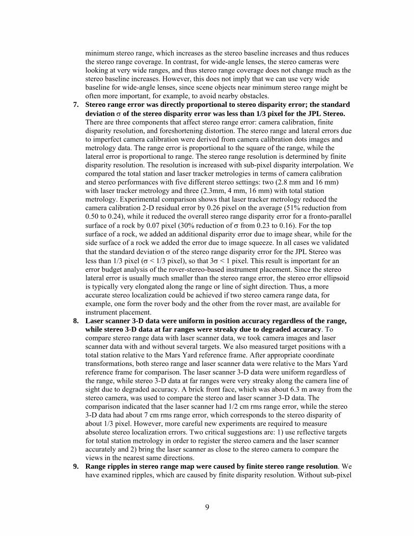
In our experiments, the most accurate 3-D metrology data were obtained by combining the laser tracker measurements of four target corners merged with the theodolite measurements of all dots of the target board (Section 2.5). Figure 5 shows the effect of using the most accurate metrology data of laser tracker all-dots (LA) as the evaluation set. The absolute magnitude of pixel error in Figure 5 is different than Figure 4 because in Figure 5 only the ten poses of the 5x5 dots target were used in the evaluation set, and the metrology method of the evaluation set was varied along with the calibration set. The 20x20 dots target poses were excluded because they did not have LA metrology data. The solid lines show the data when the calibration set and evaluation set are measured with the same measuring technique. The dotted lines show the same calibrations evaluated against the more accurate LA evaluation set. For the LT (laser tracker) calibration sets, as expected, using the LA evaluation set (LT-LA) decreased the residual error compared to the LT evaluation set (LT-LT). For the TS (total station) calibration sets, however, the LA evaluation set (TS-LA) increased the residual error compared to the TS evaluation set (TS-TS). Unexpectedly the error increased with a more accurate evaluation set. It turned out that this is due to the systematic error of imperfect alignment of the laser tracker reference frame with the total station reference frame. Only six widespread points were used for the initial reference frame alignment, causing a small systematic error between the two measurement techniques. The LA-LA (laser tracker all-dots for both calibration and evaluation sets) yielded lowest residual error of 0.1 pixel. 2.7 Volume Enclosure of the Targets

0

0.1

0.2

0.3

0.4

0.5

0.6

0.7

0.8

0.9

1

poor coverage &narrow depth

good coverage& narrow depth

poor coverage &good depth

good coverage& good depth

RMS

PIXE

L ER

ROR

hi-res 16 mm meanlo-res 2.8 mm meanhi-res 16 mm datalo-res 2.8 mm data

Figure 6. Effect of depth and image coverage of calibration target poses for the number of target poses = 3. The 16-mm narrow-angle lens was more sensitive to good depth, while the 2.8-mm wide-angle lens was more sensitive to good image area coverage.

23

In Figure 5, some combinations of target poses generated unreasonably high outliers, particularly when the number of target poses was small. Since we are interested in determining the recommended number of target poses, it is important to eliminate all “unreasonable” combinations of calibration sets from Figure 5. In order to study the effect of various combinations of target poses, we partitioned the volume enclosure of the targets into two components: depth and image coverage. The calibration targets were either at the same depth (narrow depth) or different depths (good depth), and either in the same corner of the image (poor coverage) or different corners (good coverage). Figure 6 shows the results for the case when the number of target poses was three. The plot clearly shows that the 16-mm narrow-angle lens was more sensitive to good depth, while the 2.8-mm wide-angle lens was more sensitive to good image area coverage. It appears that narrow-angle lenses require good depth to determine the focal length more accurately, while wide-angle lenses require good image area coverage to determine their nonlinearity more accurately. Residual error was in general lower with 2.8 mm because a low-resolution (640×480) CCD was used for the 2.8 mm lens while a high-resolution (1024×768) CCD was used for the 16 mm lens. For a low resolution CCD the same angular error will produce a smaller pixel error. 2.8 Number of Target Poses Based on prior studies described above, we came up with a definition for “reasonable” combinations of calibration target poses to produce camera calibration residual error plots as a function of the number of target poses. These data are useful to determine the recommended number of target poses and also for error budget analysis.

Calibration set (15 poses) o 20x20: 1, 2, 4 (1 & 2 same depth) o 10x10: 1, 2, 5, 9, 10, 12, 13 (1 & 2 same depth; 10 & 12 same depth) o 5x5: 1, 3, 5, 7, 9

Evaluation set (14 poses) o 20x20: 3, 5 o 10x10: 3, 4, 6, 7, 8,11, 14 o 5x5: 2, 4, 6, 8, 10

Constraint for “reasonable” combinations o Depth constraint: N20x20, N10x10, N5x5 ≤ (2/3) * Ntotal o Coverage constraint: Nlower-left, Nlower-right, Nupper-left, Nupper-right, Ncenter ≤ (1/2) * Ntotal

Using the “reasonable” combinations of target poses, camera calibration residual errors were computed for the high-resolution 16 mm lens in Figure 7 and the low-resolution 2.8 mm lens in Figure 8. When the number of target poses was 8, the residual error was 0.47 pixel with the total station and 0.27 pixel with the laser tracker for the high-resolution-CCD 16 mm lens, and the laser tracker reduced the residual error by 0.2 pixel. For the low-resolution-CCD 2.3 mm lens, the residual error was 0.35 pixel with the total station and 0.18 pixel with the laser tracker, and the laser tracker reduced the residual error by 0.17 pixel. The LA method was not used because we did not have LA data for the 20x20 dots target, and we felt the calibration images of that target were necessary to achieve desired depth coverage. In Figure 8, the TS method only has data points up to 9 poses because we did not have TS data for the 5x5 dots target with the low-resolution setup.

24

reasonable calibration sets (hi-res)

0

0.1

0.2

0.3

0.4

0.5

0.6

0.7

0.8

0.9

1 2 3 4 5 6 7 8 9 10 11 12 13 14 15

calibration set size

rms

pixe

l err

or

TSLT

Figure 7. Camera calibration residual error as a function of the number of target poses for 16 mm lens with hi-resolution CCD, considering “reasonable” combinations only. Laser tracker reduced the residual error by 43% (from 0.47 to 0.27 pixel with 8 target poses) compared to total station.

reasonable calibration sets (lo-res)

0

0.1

0.2

0.3

0.4

0.5

0.6

0.7

1 2 3 4 5 6 7 8 9 10 11 12 13 14 15

calibration set size

rms

pixe

l err

or

TS depth & coverageLT depthLT depth & coverage

Figure 8. Camera calibration residual error as a function of the number of target poses for 2.8 mm lens with low-resolution CCD, considering “reasonable” combinations only. Laser tracker reduced the residual error by 49% (from 0.35 to 0.18 pixel for 8 target poses).

25

2.9 Checkerboard vs. Dots MER used dots targets. The ccaldots program computes the centroid of each dot image by assuming linear perspective projection for camera image formation geometry. However, nonlinear distortion of a wide-angle lens could cause small errors in computing the centroid of each dot image. To investigate the effect of the centroid computational error, a calibration with checkerboard targets were compared with a calibration with dots targets since the checkerboard corner detector does not suffer from the centroid computational error. Experimental results (Table 2) indicated that checkerboard targets produced a bit more accurate camera calibration for a wide-angle lens tested, but only by a slight amount of 0.03 to 0.04 pixels.

Checkerboard rms pixel error Dots rms pixel error 10x10 (7 poses) 0.14 0.17 20x20 (3 poses) 0.18 0.22 All (15 poses) 0.13 0.17 Table 2. Using checkerboard targets reduced the camera calibration residual error by 0.03 to 0.04 pixels. Laser tracker measurements were used for the camera calibrations. 2.10 Camera Model (Cahv/Cahvor/Cahvore) The JPL camera calibration supports three camera models (Gennery, 1991). CAHV is a purely linear perspective projection model, where C is the camera center position vector, A is camera axis unit vector, and H and V are horizontal and vertical information vectors, respectively. CAHVOR adds correction for radial distortion, where O is optical axis unit vector and R is radial lens distortion coefficients vector. CAHVORE includes correction for fisheye distortion that adds a representation of a moving entrance pupil (the point in the lens system where light entering passes through its most narrow aperture).

Camera model 16-mm lens with hi-res (1024x768)

2.8-mm lens with lo-res (640x480)

CAHV linear model 0.41 15.63 CAHVOR nonlinear model 0.25 4.18 CAHVORE nonlinear fisheye model 0.25 0.17

Table 3. Camera calibration residual errors in pixels with three different camera models The effects of camera model for the 16-mm narrow-angle and 2.8-mm wide-angle lenses are shown in Table 3. Nonlinear distortion was less significant for the 16-mm narrow-angle. Nevertheless, the CAHVOR nonlinear model improved the calibration accuracy for both lenses. The CHAVORE fisheye model was not helpful at all for the 16-mm narrow-angle lens, but it greatly improved the calibration accuracy for the 2.8 mm wide-angle lens. Figure 9 show the ccalres residual error for the 2.8mm lens with three different camera models of CHAV, CAHVOR, and CAHVORE. The circles represent the locations of calibration target dots in the image. The lines point to the locations where the camera model says the dots should be given their 3-D coordinates. In these images the length of each line is magnified ten times. CAHV shows significant systematic errors resulting from radial distortion. CAHVOR shows errors mainly in the corners where the fisheye correction is greatest. CAHVORE shows no visible error at this magnification.

26

Figure 9. Camera calibration residual error plots magnified 10× for 2.3 mm lens: CAHV (top), CAHVOR (middle), and CAHVORE (bottom). CAHVORE yielded least residual errors.

27

2.11 Unsurveyed Calibration The JPL camera calibration is a surveyed calibration, where the 3-D positions of target dots must be known. On the other hand, un-surveyed calibration does not require 3-D metrology measurements of target poses resulting in a quite simple camera calibration procedure. It determines the camera intrinsic parameters (focal length, image center, scale, skew, radial distortion) only based on the planar uniform-spacing target pattern, and cannot determine the camera extrinsic parameters (camera position and orientation relative to the world reference frame). For this reason, camera models produced by the un-surveyed calibration procedure cannot be evaluated with the ccalres program. The current un-surveyed camera calibration procedure (Section 2.4.3), however, can determine relative positions between cameras as long as the same target poses are used for all cameras. Therefore, un-surveyed camera calibration can be used for stereo vision. We will defer comparative evaluation of unsurveyed calibration with surveyed to Section 3.17, where we compare the two calibrations through their stereo performances.

28

3. Stereo Vision A functional diagram of the JPL stereo vision software and detailed descriptions of basic software functionalities of stereo image rectification, pyramid image reduction, difference of Gaussians, stereo correlation, blob filtering, and range image generation together with CLARAty API’s can be found in Stereo Vision Technology Functional Design Document [Ansar, Kim, 2003]. 3.1 Stereo Vision Software We chose the JPL stereo vision software [Goldberg, Maimone, Matthies, 2002], which is being used for the Mars Exploration Rover (MER), as the baseline stereo vision software to test and validate. We used the CLARAty stereo vision package to run JPL Stereo within the CLARAty infrastructure. In JPL Stereo, stereo quality with high percentage of good matching or valid range pixels and stereo range accuracy is more emphasized than stereo computation speed. In particular, a novel fish-eye camera model is used to yield more accurate stereo range data for fisheye or very wide-angle lenses. In this test and validation study, we want to find what percentage of valid range pixels and what stereo range accuracy the JPL Stereo can achieve and how to produce good stereo. We also want to study the effect of various stereo parameters, which will be very useful for future stereo camera system design. Further, we want to compare with other stereo vision software. First, we have investigated the effects of correlation window size and down-sampling in terms of the percentage of good matching or valid range pixels as a stereo quality metric. In general, in a densely-textured scene, such as rocky terrain, it is best to use a small window size while in a less-textured scene, such as a sand dune, a larger window size usually works better. Down-sampling tends to yields slightly higher percentage of good matching pixels, since it becomes less sensitive to camera calibration and focus errors. Second, we have investigated the effect of epipolar misalignment on stereo correlation. The stereo correlation process in the JPL Stereo assumes zero vertical misalignment between rectified left and right images. There are, however, some vertical disparities or epipolar misalignments due to imperfect camera calibration. To see the effect of vertical misalignment, the right image was shifted by a sub-pixel amount, for example, at every 0.1 pixel over –1 to +1 pixel range, and the percentage of good matching pixels was measured. Third, we have examined the effect of defocus. Careful focus adjustment is particularly important for narrow-angle lenses or tele-photo lenses, since they are very sensitive to focus. To see the effect of defocus, either the left or right image was blurred with a Gaussian filter, and the percentage of good matching pixels was measured. Even with focus matching, we still got poor % valid range values at wide baselines for 16-mm lenses. This was due to the fact that the maximum disparity for JPL Stereo was limited to 254, which corresponded to about 5 m minimum stereo range for 16-mm lenses at the widest baseline of 30.48 cm. So the range data were cut off at about 5 m. An anomaly was observed in that we still got no range data for 16-mm lenses at full resolution (pyramid_level = 0) with wide baselines. After careful examination, we discovered that at the full resolution of pyrlevel = 0, the effective maximum disparity of JPL Stereo was in fact only 127 (minimum distance 11.2 m) not 254 (minimum distance 5.6 m). At the half resolution of pyrlevel =1 or below, max_disparity of JPL Stereo was 254. Fourth, we have studied the effect of stereo baseline. In general, wide baseline yields higher range accuracy. However, two factors usually limit the maximum baseline: minimum stereo range and stereo field-of-view or portion of the scene common to both left and right images. The effects of

29

the stereo baseline on the % valid range were measured. The stereo baseline is an important design parameter for the MSL stereo system design. Fifth, we have examined stereo range error. In general, stereo range error along the line of sight is proportional to the square of the range, while the lateral error perpendicular to the line of sight is proportional to the range. Two components affect the stereo range error: camera calibration and finite disparity resolution. The stereo range resolution is determined by finite disparity resolution, and is improved by sub-pixel disparity interpolation. We have investigated the effects of imperfect camera calibration and sub-pixel disparity interpolation on stereo range and lateral errors. Sixth, we have compared stereo range data with laser scanner data. Since the laser scanner has ½-cm resolution regardless of the range, the comparison is useful at large ranges. Seventh, we have examined ripples, which are caused by finite disparity resolutions. Without sub-pixel disparity interpolation, the range data would show as discrete lines at integer disparity values. With sub-pixel disparity interpolation, the data show a band of high-density data at and near integer disparity values. Eighth, we have examined unsurveyed calibration. The JPL camera calibration is a surveyed calibration, where the 3-D positions of target dots must be known. On the other hand, un-surveyed calibration does not require 3-D metrology measurements of target poses resulting in a quite simple camera calibration procedure. We have compared the two calibration techniques for stereo. The percentage of good match pixels with unsurveyed calibration has shown to be comparable to that with the surveyed calibration. Ninth, we have evaluated the performance of stereo with the CAHVORE fisheye camera model. For wide-angle lenses, the CAHVORE model provides more accurately rectified images for stereo than the CAHVOR model, resulting in more accurate stereo. Tenth, we have compared the JPL Stereo with SRI Small Vision System (SVS). 3.2 Test Plan The previous camera calibration experiments described in Section 2 were done indoors on a hard-floor (a raised-tile floor does not provide a stable base for the metrology equipment). By contrast, the stereo vision experiments described in this Section were done outdoors in the Mars Yard since we were interested in testing stereo vision in Mars-like terrain. Since all five high-resolution CCD cameras were not available in the previous camera calibration experiments, the stereo vision experiments required camera calibration of all five cameras first. We collected camera calibration and stereovision data for three kinds of camera lenses of 2.3 mm, 4 mm, and 16 mm. Day 1: Collect data for 4-mm lenses (fov: 65 degrees x 49 degrees)

Camera calibration o Face the stereo camera head holding five 4-mm cameras straight forward at 1.5 m

high o Move the dots target board at 16 different poses using a target stand. For each

target pose, collect camera images from all five cameras, and measure the reference target positions on three corners of the target board using a total station.

o 8 target poses for calibration

30

6 distances (2 close and 4 medium) with the 10x10 target 2 far distances with the 5x5 target

o 8 other target poses for evaluation to compute the residual error of the camera calibration obtained

6 distances (2 close and 4 medium) with the 10x10 target 2 far distances with the 5x5 target

o Save image files as hi4_10x10d[1-12]_[A-E] (6 calibration and 6 evaluation images for each

of 5 cameras of A through E) hi4_5x5d[13-16]_[A-E] (2 calibration and 2 evaluation images for each

of 5 cameras of A through E) Panoramic image collection

o 2 tilts about –20° and –40°

o 5 pans for each of the two tilts about –100°, –50°, 0°, 50°, 100°

o Just collect images (neither total station nor laser scanner measurements) an example of a filename: hi4_neg20tilt_neg50pan.pgm

Range calibration o Place the stereo camera head at 0° pan and –20° tilt o Place 5 to 7 post-it display 2×2 checkerboard (single intersection) targets o Make total station measurements of each target position o Take camera images with post-it targets

hi4_with_targets.pgm o Take laser scanner data with post-it targets o Remove post-it targets and take camera images

hi4_no_targets.pgm o Remove camera tripod and take laser scanner data without post-it targets o Pick 5 salient flat regions and take 4 to 5 position measurements (e.g., 4 corners

of a square and its center) for each of the five regions Day 2: Collect data for 2.3-mm lenses (fov: 113 degrees x 86 degrees)

Camera calibration Panoramic image collection (2 tilts; 3 pans) Range calibration All above procedures are essentially same as Day 1.

Day 3: Collect data for 16 mm lens (fov: 17 degrees x 13 degrees)

Camera calibration Panoramic image collection (4 tilts, 11 pans) Range calibration All above procedures are essentially same as Day 1.

3.3 Experimental Setup For the stereo camera head, a solid one-piece faceplate (Figure 10) was fabricated that holds up to 5 CCD’s on one side and 5 CS-mount lenses on the other side, maintaining high mechanical stability between the cameras. The stereo-head faceplate supports 7 different baselines from 7.62 cm (3 in) to 30.48 cm (12 in) at every 3.81 cm (1.5 in).

31

7.62 cm (3”) 7.62 cm (3”) 11.43 cm (4.5”) 11.43 cm (4.5”) Figure 10. The faceplate design for the stereo camera head, supporting 7 different baselines simultaneously from 7.62 cm (3 in) to 30.48 cm (12 in) at every 3.81 cm (1.5 in) Five high-resolution firewire Dragonfly cameras manufactured by Point Grey Research were used for the experiments. The high-resolution cameras provide 1024 pixels × 768 pixels images. Three kinds of lenses were used in the experiment: wide-angle 2.3 mm lenses with a 113°×86° field of view (FOV), 4 mm lenses with a 65°×49° field of view, and 16 mm lenses with a 17°×13° field of view. Table 4 summarizes the lenses used.

Focal length Horizontal FOV × Vertical FOV

Computar 2.3 mm 113° × 86°

Fujinon 4 mm 65° × 49°

Fujinon 16 mm 17° × 13° Table 4. Lenses used for the stereo vision experiments

The images were collected using a laptop computer with an OrangeLink firewire card-bus PC card. The Point Gray’s Dragonfly Image capture software was modified to support the consecutive acquisition of the stereo images with new filenames. A firewire hub was used to allow up to 5 cameras to be connected to the computer simultaneously. For the camera calibration two target boards were used: 10×10 and 5×5 dots targets. Both targets were of the same size, 112 cm × 112 cm (44 in × 44 in). A target stand was used to facilitate positioning of the target boards. A Leica TPS 1100 total station were used to measure the target board poses. The total station measured reflective target positions at three corners of the target board. The metrology accuracy of the total station used in this stereo vision experiment was 2 mm. Note that in the previous camera calibration the total station was from the JPL metrology service and was more accurate with a 0.5 mm measurement accuracy. A Riegl laser mirror scanner LMS-Z360 was used to collect 3-D terrain maps. Its measurement accuracy is typically 1σ = 1.2 cm. 3.4 Total station procedure Unlike the previous camera calibration experiments, we used a total station ourselves in this Mars Yard stereo vision experiment. This required additional knowledge of how to set up the total station and how to perform coordinate transformations to compute the dot positions. The following procedure sets up the total station such that its measurements are relative to the Mars Yard reference frame. Setting up the Total Station (provided by Tara Estlin and Daiel Gaines)

32

A. Level the Station · Level bubble on base of total station by adjusting tripod legs and black knobs · Turn on Station by pressing on button · Hit shift+head- light button · Adjust circles by adjusting black knobs · Hit Cont (F1)

B. Set Station Orientation · You Should be at Main Menu · Hit Setup (F5) · Hit New Job (F2) · Enter Job name · Hit Cont (F1) · Hit Stn (F1) · Set Station Id to 0 · Set everything else to 0:

a. Inst Height b. Stn N c. Stn E d. Stn Elev

· Hit Set Hz (F4) · Hit Set Hz to 0 (F4) · Hit Record (F3) · Hit Cont (F1) · Hit Prog · Select Tie Distance · Point Station at Origin Target in Mars Yard · Enter Point ID of 1 · Hit All (F1) · Point Station at +X Target in Yard (should automatically set Point ID to 2) · Hit All (F1) · Tie Distance should be automatically calculated · Make a note of Azimuth (Az) value · Hit Esc until back at “Enter Station Data” screen (should be 3-4 times) · Turn Station until Hz = 0 · Hit Set Hz (F4) · Enter 360-(Azimuth value previously collected) · Hit Set (F1) · Hit Esc – Should be at “Job Settings”

C. Set Station Coordinates · Hit Meas (F6) · Point Station at Origin Target · Hit Dist (F2) · Scroll down using arrow keys · Record N, E, and Elev · Hit Esc (should be back at “Job Settings”) · Hit Stn (F1) · Change Station ID to 1 · Enter negative of recorded E and N values · For height, enter 3 – (recorded elevation value) · Hit Record (F3)

D. Verify Yard Targets

33

· Origin a. E = 0.000 b. N = 0.000 c. H = 3.000

· Plus Y a. E = 0.001 b. N = 17.540 c. H = 2.401

· Plus XY a. E = 20.419 b. N = 17.559 c. H = 2.140

· Plus X a. E = 20.458 b. N = 2.598 c. H = 0.853

The ccaldots program needs .fix file that specifies four corner dot positions. There are two ways to get these data. The first is to use the total station to directly measure these four corner dot positions. The second method is to use the total station to measure the reflective reference target positions on the corners of the target board, and then compute the four corner dot positions by appropriate coordinate transformations. We decided to use the second method, since we were not sure how accurate the total station measurements were with non-reflective surfaces. The following procedure does appropriate coordinate transformation by least-squares method to compute four corner dot positions from three reference target point measurements. Procedure to compute four corner dot positions:

Read the total station metrology .GSI file by using the Leica SurveyOffice Coordinate Editor, and convert the .GSI file to an ASCII text file (e.g., in_file).

Create a target board calibration text file (e.g., target_board_file) that tells you the geometric relations between corner target positions and corner dot positions.

Finally, start Matlab and run: ts_target(target_board_file, in_file, start_row, num_poses, out_file)

The start_row and num_poses parameters are determined by looking at the total station log (a hand-written note or .doc file) that tells you which point ID’s are for corner target positions.

To compute 10x10 corner dots, for example, run ts_target('TS_10x10D.txt', 'IPTASK.txt', 2, 12, 'fix_10x10D.txt');

To compute 5x5 corner dots, for example, run ts_target('TS_5x5D.txt', 'IPTASK.txt', 38, 4, 'fix_5x5D.txt');

Once 3-D positions of corner dots are obtained, enter these data to the target .fix files. 3.5 Laser Scanner Procedure The laser scanner installation and run procedure is summarized here.

Configure the laptop computer’s parallel port in the ECP mode Install the Riegl’s RiPort driver on the laptop computer Install the Riegl’s 3D-RiSCAN software on the laptop computer.

34

Connect the Riegl laser scanner to the parallel port and the serial port of a laptop computer. These connections are on the bottom of the laser scanner.

Power up the laser scanner and the laptop. Run ‘3D-RISCAN’ to capture and store the data from the laser scanner. To perform a

scan, use the ‘Define’ tab from the program’s main menu to specify the scanner parameters. Thereafter press the ‘Start Acquisition’ radio button pressed to begin the scan. After the scan has been completed, save the data by selecting the ‘File’ tab. A user documentation is available from the ‘Help’ tab of the program.

3.6 CLARAty Stereo Vision Procedure The CLARAty stereo vision package provides an infrastructure to support several different vision modules. At present it supports JPL Stereo and SRI SVS modules. Here is the procedure on how to download. Compile, and run test_jpl_stereo. To check out the CLARAty stereo vision package from the CLARAty repository,

tcsh // csh causes an error klog user_name // enable access of /afs files start_clarity // set environmentalvariables) yam setup –nolink –nobuild –d dir_name

and when YAM.config comes up, edit it as follows, or just copy and paste WORK_MODULES, LINK_MODULES, and BRANCH* from /home/marstech/IPvalidation/stereo/clarity/jpl_initial/YAM.config.

WORK_MODULES = stereo_vision_jpl \

stereo_vision_svs \ jplpic

LINK_MODULES = SiteDefs/SiteDefs-R1-10j \ arrays/arrays-R1-08 \ camera_image/camera_image-R1-04 \ camera_model/camera_model-R1-04 \ camera_model_jpl/camera_model_jpl-R1-01 \ frame/frame-R1-06 \ image/image-R1-04-Build01 \ image_io/image_io-R1-03-Build01 \ image_ops/image_ops-R1-04 \ matrices/matrices-R1-09 \ numerics/numerics-R1-01a \ point_cloud/point_cloud-R1-02 \ points/points-R1-08 \ share/share-R1-09 \ stereo_processor/stereo_processor-R1-03-Build01\ string_io/string_io-R1-02a-Build01 \ transforms/transforms-R1-07-Build01

BRANCH_stereo_vision_jpl = stereo_vision_jpl-R1-03 maxb BRANCH_jplpic = jplpic-R1-01 wonsoo BRANCH_stereo_vision_svs = stereo_vision_svs-R1-03 wonsoo

35

To compile: cd dir_name gmake yam-mklinks gmake links gmake libs cd src/jplpic ymk all // compile jplpic source codes cd ../stereo_vision_jpl ymk all // compile stereo_vison_jpl source codes to create test_jpl_stereo

To run test_jpl_stereo:

Make a directory, e.g., data2, under src/stereo_vision_jpl. Under the data2 directory, populate cahvor files and image files if you want. Otherwise, simply create script files and read files from other directories. Here is an example run.

../sparcSol2.7/test_jpl_stereo left.pgm right.pgm left.cahvor right.cahvor 0 9 254

The last three numbers are pyramid level, correlation window size, and maximum disparity, respectively. The pyramid level 0 means no image reduction or down-sampling, 1 means image reduction by half in each dimension, and 2 means image reduction by a quarter in each dimension. The blobsize defines the size of range patches to ignore as noise

The test_jpl_stereo program provides a wrapper interface to run the JPL Stereo software module within the CLARAty environment. Although JPL Stereo supports dozens of command line options, CLARAty users can modify the CLARAty interface software according to their needs. In our applications, the test_jpl_stereo interface was modified to support the following inputs and outputs. The test_jpl_stereo program runs JPL Stereo internally, which takes a stereo pair of images with associated camera models and generates a range image with respect to the left camera. test_jpl_stereo left_image right_image left_model right_model \

pyrlevel windowsize maxdisp blobsize

The following are the input parameters. left_image and right_image: pgm files left_model and right_model: camera models (cahv, cahvor, cahvore2)

generated during calibration pyrlevel: image reduction level before stereo processing.

0 corresponds to no reduction, 1 to reduction by half in each dimension, 2 by a quarter, etc.

windowsize: correlation window size maxdisp: maximum disparity search range blobsize: size of range patches to ignore as noise

36

After the run, test_jpl_stereo produces the following outputs. result.ran: range image consisting of a header followed by x, y, z coordinates of

3-D points corresponding to each pixel. The coordinates are float. By convention, a missing range value has (x,y,z)=(-100000, -100000, -100000).

l-rect.cahv: linearized (non-radial distortions removed and scale adjusted) and rectified camera model for the left camera

r-rect.cahv: linearized and rectified camera model for the right camera l-rect.pgm: linearized/rectified left image associated with l-rect.cahv r-rect.pgm: linearized/rectified right image associated with r-rect.cahv disparity.pgm: disparity image range.pgm: range image

3.7 Stereo Vision Analysis Tools The JPL rangediag program was used as a generic stereo test tool to view and examine the outputs of test_jpl_stereo. The program is used as follows:

rangediag [opt] result.ran l-rect.cahv l-rect.pic The most relevant options are

-r: sets range interval to display (e.g. –r1,10) -h: sets height interval to display (e.g. –h-3,5) -f: sets forward vector (e.g. –f1,2,1) -g: sets ground point (e.g. –r0,0,-2)

These switches effect the display and color scheme and are generally not needed. The output of rangediag is a diagnostic image consisting of 5 parts.

Upper left: The range map, with range encoded by color Upper center: The normal intensity image Upper right: The height image, with height encoded by color Center: An overhead view of reconstructed pixels, with height encoded by color Bottom: A sidways looking profile.

Clicking on any pixel in any of the screens displays range and height information and updates the bottom screen to display the range profile at the given pixel. Several MATLAB codes have been developed for stereo analysis. To investigate the effect of vertical misalignment, we used shift.m to shift an image vertically by a sub-pixel. shift (‘image.pgm’). To investigate the effect of defocus or blur, we used blur.m to blur an image with a Guassian filter. blur (‘image.pgm’). To investigate vertical misalignment between rectified left and right images due to imperfect camera calibration, we used vert_disp.m that compute the vertical disparity or misalignment of the left and right dot positions in the rectified left and right images by using the calibration target dots files obtained from ccaldots. vert_disp (‘EB_E.dots’, ‘EB_B.dots’).

37

To compute the stereo range and lateral errors due to imperfect camera calibration, we used testStereo.m that computes and plots the range and lateral errors by using rectified camera models and camera calibration dots files. test_stereo (‘l-rect.cahv’, r-rect.cahv’, ‘EB_E.dots’, ‘EB_B.dots’). To compute the stereo range resolution due to sub-pixel disparity interpolation, we used h_shift.m and hor_disp.pl.

When a camera was moved from the calibrated position, e.g., to new pan and tilt angles, the stereo range data need to be transformed. Several MTALB codes were used to perform appropriate transformations for the camera and the laser scanner. 3.8 Image Down Sampling One option of the JPL Stereo algorithm is to process stereo images at reduced resolution. A pyramid level of 1 treats each 2x2 window of pixels as a single pixel, averaging their values. Thus, it reduces the image size to a half in each dimension. A pyramid level of 2 reduces the image size to a quarter in each dimension. In general, one level of down-sampling reduces the computational time of the stereo correlation by a factor of 8 as described in Section 3.19. It also makes the stereo correlation less sensitive to camera calibration and focus errors as described in Section 3.10 and 3.11. The drawback is that it reduces the stereo range resolution. Specific effects of down sampling with respect to our evaluation variables are described throughout Section 3. 3.9 Correlation Window Size The correlation window size affects the stereo correlation performance. Too large or too small window sizes will yield a poor percentage of the valid range. In general, a densely textured scene, such as a rocky terrain, performs better with a smaller window size, while a less-textured scene, such as a sand dune, usually works better with a larger window size. We investigated the effect of varying the correlation window size. First we compared the range data outputs obtained with two different window sizes of 7×7 pixels (Figure 11) and 15×15 pixels (Figure 12) for 4-mm lenses at full resolution (pyramid_level=0). The smaller 7×7 window produced range data with more fine details. For example, it produced valid range data for the “thin” arm at the top of the lighting pole in Figure 11, while the larger 15×15 window missed it in Figure 12. Further, the larger window produced a much fatter lighting pole due to the foreground fattening effect, where a textured foreground tends to be fattened over a less-textured background for the non-shiftable rectangular window correlation. However, the larger 15×15 window produced better range data for less-textured regions such as the mountain on the right hand side of the image and the dots target board. The above observations clearly indicate that the window size affects the valid range percentage. Figure 13 is the range data plot obtained after down-sampling by 1 level at pyramid_level =1. The window size used was 7×7 pixels at half resolution, which corresponds to approximately 15×15 pixels at full resolution of Figure 12. For this reason, the range data plots of Figures 12 and 13 show great similarity except one main difference. Figure 13 has four times sparse range data (2 times sparse in each dimension), whose stereo range resolution is lowered by a factor of two. It also shows range ripples, which are described in more detail in Section 3.16.

38

Figure 11. Stereo range map using a 7×7 correlation window at pyramid level 0 (full resolution) for 4-mm lenses: smaller window size produces the range map with fine details such the “thin” arm at the top of the lighting pole.

Figure 12. Stereo range map using a 15×15 correlation window at pyramid level 0 (full resolution) for 4-mm lenses: larger window size handles low-texture regions better such as the dots target board and the mountain at the right hand side.

39

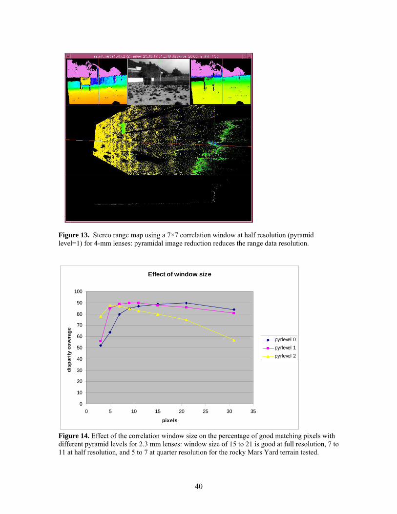
Figure 13. Stereo range map using a 7×7 correlation window at half resolution (pyramid level=1) for 4-mm lenses: pyramidal image reduction reduces the range data resolution.

Effect of window size

0

10

20

30

40

50

60

70

80

90

100

0 5 10 15 20 25 30 35

pixels

disp

arity

cov

erag

e

pyrlevel 0pyrlevel 1pyrlevel 2

Figure 14. Effect of the correlation window size on the percentage of good matching pixels with different pyramid levels for 2.3 mm lenses: window size of 15 to 21 is good at full resolution, 7 to 11 at half resolution, and 5 to 7 at quarter resolution for the rocky Mars Yard terrain tested.

40

We measured the % valid ranges as a function of the correlation window size with different image reduction pyramid levels for 2.3 mm (Figure 14). The figure shows that the correlation window size of 15 to 21 is good at full resolution, 7 to 11 at half resolution, and 5 to 7 at quarter resolution for the rocky Mars Yard terrain. Interestingly this result seems to suggest the ratio of the optimal correlation window size to the image size is roughly constant over different image reduction pyramid levels. At full resolution, however, window size of 9 is probably preferred to 15 or 21 to reduce the foreground fattening effect, even though window size of 15 or 21 yields slightly higher percentage of good match pixels. 3.10 Vertical Image Shift To search for correlated pixels, JPL Stereo produces a rectified image pair where the two images are vertically aligned. This alignment relies on the accuracy of the camera model. To test the effect of vertical misalignment we shifted one image of a pair vertically to produce an error in the vertical alignment. Experimental results (Figure 15) show that there is a plateau in the middle where a small amount of vertical error does not hinder the ability of the algorithm to find correlated pixels. The ±0.5 pixel vertical misalignment from the center of the plateau (-0.6 pixel to 0.4 pixel) reduces the percentage of good matching or valid disparity pixels from 86% to 75%, or mere 13% reduction from the maximum. However, a greater amount of vertical misalignment produces significant deterioration of stereo correlation. The ±1 pixel vertical alignment error reduces the percentage of valid disparity pixels by 50%. Increasing the pyramid level by 1 broadens the plateau width by a factor of 2, indicating that down-sampling makes the stereo correlation less sensitive to vertical misalignment. Vertical misalignment errors of our camera calibrations were typically about 0.1 to 0.2 pixel, which would not deteriorate the percentage of valid disparity pixels significantly. However, they can moderately contribute to stereo disparity error as described in Section 3.14.

Effect of vertical shift

0

10

20

30

40

50

60

70

80

90

100

-1.5 -1 -0.5 0 0.5 1 1.5

pixels

disp

arity

cov

erag

e

pyrlevel 0prylevel 1pyrlevel 2

Figure 15. Effect of vertical shift on the percentage of valid disparity pixels: ±0.5 pixel vertical misalignment starts to degrade the stereo correlation performance noticeably.

41

3.11 Image Blur Good focus of the individual cameras is vital to stereo performance. We found this to be especially true for narrow field of view cameras, which are mechanically very sensitive to focal adjustment. In early testing we discovered that two cameras defocused by the same level performed better than if one of them was well focused. To investigate this we determined the worst focused camera. We then blurred the images from the other cameras by varying amounts and plotted stereo performance against blur.

Blur all cameras to match camera A

0

10

20

30

40

50

60

70

80

90

0 0.2 0.4 0.6 0.8 1 1.2 1.4 1.6

gaussian blur standard deviation

disp

arity

cov

erag

e

Camera BCamera CCamera DCamera E

Figure 16: Effect of image blur on stereo correlation, 2.3mm lenses: camera A was not in good focus, and thus other four cameras from B to E needed to be defocused to the same level as camera A to get good stereo correlation.

Figure 17: A well-focused camera C image (left) and a defocused camera A image (right) – 2.3 mm lenses.

42

Figure 16 of a 2.3 mm example, indicates that camera A is defocused, while the other four cameras from B to E are in the same level of good focus. Cameras B to E need to be blurred by the Gaussian blur filter with σ = 0.8 pixel to get the maximum percentage of valid disparity pixels, where σ is the half width of the blurred point image or point spread function. Noting that the half of one pixel width is 0.5 pixel, σ = 0.8 pixel implies that it blurs each image pixel roughly by 0.3 pixel more from the center of the pixel, resulting in 1.6 pixel blur size. Figure 17 compares a well-focused Camera C image with a defocused Camera A image.

Blur camera C to match camera B

0

10

20

30

40

50

60

70

80

90

100

0 1 2 3 4 5

gaussian blur standard deviation

disp

arity

cov

erag

e

Pyralmid Level 0Pyramid Level 1Pyramid Level 2Pyramid Level 3

Figure 18. Effect of image blur on stereo correlation, 16mm lenses: camera C needed to be defocused to match with camera B. Stereo matching in lower resolution using a higher pyramid level with a greater image reduction is less sensitive to focus mismatch.

Figure 19. A well-focused camera C image (left) and a defocused camera B image (right) – 16 mm lenses.

43

In Figure 18 of a 16 mm example, Camera C needed to be blurred with σ = 1.5 pixel to produce the maximum stereo disparity percentage. Blurring the image, making it worse, can actually improve stereo performance up until the point where the blur matches the other camera. Beyond this point, blur degrades performance. The ±0.5 pixel change of σ (1 < σ < 2 pixels in Figure 18) at full resolution did not change the stereo disparity percentage too much. At half resolution (pyramid level = 1), the plateau width doubled to about ±1 pixel. Without the blur, stereo correlation at full resolution resulted in an empty disparity map. Figure 19 compares a well-focused Camera C image with a defocused Camera B image. 3.12 Maximum Disparity The algorithm to find pixel correlation searches between minimum and maximum disparity values. The larger the search, the slower the algorithm is. The maximum disparity determines the minimum range at which correlation can be detected.

0.0

0.5

1.0

1.5

2.0

2.5

3.0

3.5

4.0

4.5

5.0

0 10 20 30 40STEREO BASELINE (cm)

MIN

IMU

M S

TER

EO R

ANG

E (m

)

2.3 mm4 mm16 mm

Figure 20. Minimum stereo range computed as a function of stereo baseline for three different camera lenses (2.3 mm, 4 mm, and 16 mm) with the maximum disparity of 254 pixels, with the horizontal image size of 1024 pixels. Actual camera focal lengths are slightly different from the nominal lens focal lengths used in this plot. Figure 20 shows the relation between baseline, focal length, and minimum stereo range for a maximum disparity of 254 pixels, with the horizontal image size of 1024 pixels. This corresponds to 75% overlap between the left and right images. The values are related as follows:

• Rmin = Fs * B / Dmax • Fs = 1024 pixels * F / 4.4 mm

Rmin is the minimum stereo range, Fs is the camera’s horizontal focal length in pixels, B is the baseline, Dmax is the maximum disparity, and F is the camera’s focal length. The horizontal image size of the 1/3” CCD format is 4.4mm.

44

3.13 Stereo Baseline Increasing stereo baseline reduces range error. However, it also reduces the percentage of valid disparity pixels. There are several reasons why the percentage would be reduced. The stereo overlap area becomes smaller as the disparity value increases. For instance, at the maximum disparity for 254 for the horizontal image size of 1024 columns, the stereo overlap is 75%. Increasing stereo baseline also increases the stereo minimum range as described in the previous Section, limiting the closest object that can be found. And by viewing at the same object from different angles, two projected camera images of the object are slightly different in shapes,

Figure 21. The percentage of valid disparity pixels

reducing the stereo correlation performance.

s as the stereo ver,

Figure 22. After the blur correction for stereo, two abnormal dips disappeared. The disparity coverage at pyramid level 2 was shown slightly lower than at pyramid level 1, because a larger effective area of the image boundary was eliminated from stereo matching.

0102030405060708090

100

5 10 15 20 25 30

STEREO BASELINE (cm)

DIS

PAR

ITY

CO

VER

AGE

(%)

pyrlevel 0pyrlevel 1pyrlevel 2

in general slightly decreasebaseline increases, for the 2.3 mm lens tested. In the initial result before blur correction, howetwo abnormal dips at pyramid level 0 appeared.

0102030405060708090

100

5 10 15 20 25 30STEREO BASELINE (cm)

DIS

PAR

ITY

CO

VER

AGE

(%)

pyrlevel 0pyrlevel 1pyrlevel 2

45

Figure 21 shows an initial experiment with the 2.3mm lenses, which was not corrected for blur. The 15.24mm and 26.67mm baselines used camera A that had the worst focus. This reduced stereo performance for those specific baselines. From this graph we can also see the pyramid image reduction makes the stereo correlation less sensitive to focusing error. The results after correcting for blur (Figure 22) indicate only a weak correlation between increased baseline and reduced percentage of valid disparity pixels. This is because a wide-angle lens tends to cover a wide range of object distances, and only a small image portion in closer ranges is affected by the increased baseline. A slight increase in disparity value at far ranges has almost no effect on the stereo overlap percentage. Figure 23 shows the results of baseline on the 16mm lenses. The percentage of the valid disparity pixels drops as baseline increases, and this drop is steeper than with the 2.3 mm lenses. This is because a narrow-angle lens tends to cover a narrow range, and in our 16-mm tests the object distance from the stereo camera happened to be around the minimum stereo range. Note that objects at far ranges hardly affect the stereo overlap percentage. Then there is a sudden drop with large baselines as the minimum stereo range further increases to start to cut down the valid

cts y

bug that limits maximum disparity to 127 instead of 254. Details are described in Section 4.2. Overall, it seems safe to increase baseline as long as the area of interest is in the field of view of both cameras and at greater than the minimum stereo range.

disparity image area. When the baseline = 30.48 cm (12 in), only a very small fraction of objewas beyond the minimum stereo range, and thus the percentage of valid disparity pixels was versmall. The pyramid level 0 data in Figure 23 show the effect of the software

0.0%

10.0%

20.0%

30.0%

40.0%

50.0%

60.0%

70.0%

80.0%

90.0%

100.0%

0 10 20 30 40

Baseline (cm.)

Dis

parit

y C

over

age

Pyramid Level 0Pyramid Level 1Pyramid Level 2Pyramid Level 3

Figure 23. The disparity coverage dropped rapidly as the stereo baseline increased, for the 16 mm lens tested because wide baselines could not produce stereo range below the minimum stereo range. The pyramid level 0 data (dark blue) show the effect of the software bug that limited the maximum disparity to 127 instead of 254. More details are described in Section 4.2 and 5.

46

3.14 Stereo Localization Error We will now derive the relationship of the stereo 3-D localization error to the image disparity error. Figure 24 shows a pair of stereo cameras. Due to similar triangles (one with B in dashed

ne and the other with d, respectively, in Figure 24):

t 24, the plane will show up as a line parallel to

e x-axis. Differentiating (2) and then substituting (3) for d, we get:

or the lateral error, we consider adding ∆x for both left and right image points (∆x1 = ∆x2 = x). From similar triangles (one with ∆X and the other with ∆x, respectively, in Figure 24):

(11) Z / f = ∆X / ∆x (12) ∆X = (Z / f) ∆x

The lateral error ∆L perpendicular to the range error ∆R is related to ∆X by: (13) ∆L = ∆X cosθ

li(1) Z / f = B / d (2) Z = f B / d (3) d = f B / Z

The above equations imply that the constant disparity d corresponds to a fronto-parallel plane, noa sphere, at a distance Z along the z-axis. In Figureth

(4) ∆Z = −f B ∆d / d2 (5) ∆Z = −(Z2 / f B) ∆d

The negative sign appears because Z decreases as d increases. The range R is related to Z by (6) Z = R cosθ (7) ∆R = ∆Z/cosθ

From (5)-(7), (8) ∆R = −(R2 cosθ / f B) ∆d (9) ∆R ≈ − (R2 / f B) ∆d (10) |∆R| ≈ (R2 / f B) |∆d|

In Figure 24, the range error ∆R is along the line of sight, where −∆d is added for the right image only (∆x1 = 0; ∆x2 = −∆d). F∆

B

Z

θ

df

R

∆R

∆x2 ∆x1

∆L

∆X

∆Z

B

Figure 24. Geometry for Stereo localization error analysis

47

From (6), (12), and (13), 2(14) ∆L = (R cos (θ) / f) ∆x

y). ∆R) ≈ ∆R / R

Fro −∆d,

or is quadratic with range whi

ion for the right image point. Since the disparity is the difference between left and right image point, x1 a

d = x1 – x2 The

Fro

or is directly related to the difference of ∆x1 and ∆x2. On the other and, the average error common to both delta x1 and delta x2, that is (∆x1 + ∆x2) / 2, does not

e on

erro ponen ute the stereo lateral error. From (15), + ∆x2) / 2

known, the stan eviati ereo 3-D reconstruction range error can be computed by

(23) σ∆R = (R2 / f B) σ∆x1 – ∆x2 When the standard deviation σ(∆x1 + ∆x2) / 2 of the stereo 2-D re-projection error are known, the standard deviation σ∆L for the stereo 3-D reconstru on lateral error can be computed by

(24) σ∆L = (R / f) σ(∆x1 + ∆x2) / 2 In general, we can conceive an error ellipsoid in 3-D space bounded by the range and lateral errors of (23) and (24). Since the camera calibration process produced the 3-D metrology data of the calibration dot positions and their associated 2-D image points, we can c pute the 3-D localization error for each dot position by comparing the metrology-based 3-D position and the reconstructed 3-D position from the 2-D image point pair based on the stereo camera models. By contrast, me uring 3-D positions from a natural terrain is more difficult. Figures 25 and 26 show overhead views of dot positions of calibration targets and their 3-D reconstruction error for 16 mm with laser tracker metrology and for 2.3 mm with total station metrology. The cameras were located at the red square+triangle camera symbols. Each blue line extends from a calibration dot’s true position towards its stereo reconstructed position. The lengths of the lines have been magnified for visibility, but their direction and relative lengths are correct. The magnification was 20 for Figure 25 and 100 for Figure 26. From this we can see that points closer to the cameras have less error, and the direction of the error tends to be along the

be a lot larger thanelongated along the line of sight.

(15) ∆L ≈ (R / f) ∆x We can also derive the stereo range error formula geometrically by using similar triangles (one with B in solid line and the other with ∆X, respectivel

(16) ∆X / B = ∆R / (R + m (10) and (15) with ∆x = (17) −(Z / f B) ∆d = ∆R / R (18) ∆R = −(R Z / f B) ∆d = −(R2 cosθ / f B) ∆d

(18) is the same as (8). For the stereo range error computation we use (10), and for the stereo lateral error computation we use (15). From this we see that range err

le lateral error is only linear.

Now we consider a general case with a ∆x1 variation for the left image point and a ∆x2 variat

nd x2 respectively, (19) refore (20) ∆d = ∆x1 – ∆x2 m (9) and (20), (21) ∆R = − (R2 / f B) (∆x1 – ∆x2)

Note that the stereo range errhchange the disparity d. From (2), no change in d means no change in the z-axis distance Z. Sinc∆R is in general not along the z-axis, there is a small coupling but can be ignored. The comm

r com t is used to comp(22) ∆L = (R / f) (∆x1

When the standard deviation σ∆x1 – ∆x2 of the stereo 2-D re-projection error aredard d on σ∆R for the st

cti

om

as

line of sight from the camera. This suggests that the stereo range errors tend to the lateral errors, and thus the error ellipsoid becomes very

48

Figure 25. Overhead view of stereo 3-D localization errors of calibration dots for 16 mm lens,

gy: stereo localization error is directed strongly along the range. Each blue line 0× ma on from metrology and the 3-D laser tracker metrolo

is a 2 gnified position error between the true 3-D positiposition reconstructed from the corresponding 2-D image point pair.

Figure 26. Overhead view of stereo 3-D localization errors of calibration dots for 2.3 mm lens,

total station metrology: each blue line is a 100× magnified position error. Figures 27 and 28 show an analysis of range error for the same data sets. Each + is a calibration dot which is plotted by range from the cameras against range error. The red solid curve is theexpected error computed by using (22) together with the differential error σ∆x1 – ∆x2, which was obtained by comparing the 2-D reprojections of calibration dot 3-D points from metrology and their corresponding 2-D image points. The measured 3-D localization error agrees well with expected error predicted by (22). The black dashed curve is the expected 3-D localization error for a disparity rms error of one pixel. Figures 29 and 30 are the same data set plotted against

49

lateral error using (23) together with the common error σ(∆x1 + ∆x2) / 2. Again, the measured 3-D localization error agrees well with the expected 3-D error predicted by (23).

Figure 27. Range error caused by camera calibration inaccuracy; 16mm lens, laser tracker metrology. Red solid curve: σ = 0.16 pixel. Black dashed curve: σ = 1 pixel. ∆x1 – ∆x2 ∆x1 – ∆x2

Figure 28. Range error caused by camera calibration inaccuracy; 2.3mm lens, total station metrology. Red solid curve: σ∆x1 – ∆x2 = 0.12 pixel. Black dashed curve: σ∆x1 – ∆x2 = 1 pixel.

50

Figure 29. Lateral error caused by camera calibration inaccuracy; 16mm lens, laser tracker

. metrology. Red solid line: σ(∆x1 + ∆x2) / 2 = 0.24 pixel. Black dashed line: σ(∆x1 + ∆x2) / 2 = 1 pixel

Figure 30. Lateral error caused by camera calibration inaccuracy; 2.3mm lens, total station

. metrology. Red solid line: σ(∆x1 + ∆x2) / 2 = 0.21 pixel. Black dashed line: σ(∆x1 + ∆x2) / 2 = 1 pixel

51

So far, we examined the stereo vision 3-D location error caused by camera calibration inaccuracy only. Camera calibration inaccuracy is, however, not the only source of the 3-D localization error. Stereo correlation inaccuracy is another source of error. Stereo correlation determines the disparity between left and right images for each pixel, and the disparity determines the 3-D location by triangulation. The JPL stereo correlation employs the quadratic sub-pixel disparity interpolation, where correlation scores at three adjacent disparity values are used to estimate the disparity value at sub-pixel level, This sub-pixel disparity interpolation improves the accuracy of the stereo disparity estimate, but still yields some inaccuracy. To evaluate the inaccuracy of the sub-pixel disparity interpolation, we shifted the left image by an integer plus some sub-pixel amount (Figure 31), and compared the stereo correlator output disparity with the actual image shift. The horizontal image shift corresponds to the case when a fronto-parallel planar surface moves back or forth. If the stereo correlator were perfect, every pixel would register a disparity equal to the actual amount of the shift. By observing deviations from the correct disparity we can estimate the amount of subpixel error introduced by the stereo correlator sub-pixel interpolation. The results (Figure 32 left side) indicate that the sub-pixel quadratic interpolation has the bias error in estimating the sub-pixel disparity value. The bias tends to be towards the nearest integer disparity, and is about 0 at the disparity with the 0.5 fraction. Due to a large bias value at 0.25 fraction, the rms error of the disparity estimate relative to the actual value yields double humps (Figure 32 right side). The disparity rms error over all integer and fractional disparities was 0.11 pixels in this example test.

Figure 31. Horizontal image shift corresponds to the case when a fronto-parallel planar surface moves back or forth.

tion

(cm)

-0.15

-0.1

-0.05

0

0.05

0.1

0.15

8 8.2 8.4 8.6 8.8 9

horizontal image shift (pixels)

disp

arity

bia

s er

ror (

pixe

ls)

-0.15

-0.1

-0.05

0

0.05

0.1

0.15

8 8.2 8.4 8.6 8.8 9

horizontal image shift (pixels)

disp

arity

rms

erro

r (pi

xels

)

Figure 32. Disparity bias error (left) and rms error (right) of the sub-pixel disparity interpolaalgorithm, obtained by varying the amount of horizontal image shift.

52

Vertical misalignment caused by imperfect camera calibration also affects the stereo disparity estimate. To investigate the effect of vertical misalignment, the left image is shifted both horizontally and vertically (Figure 33). Whole-number horizontal shifts show the effect of vertical misalignment only, while fractional shifts show the effect of both sub-pixel interpolaand vertical misalignment.

tion Figure 34 shows the effect of horizontal and vertical shift on the

bility to find good matching pixels. From the separate curves we see the effect of vertical shift

areducing the number of good matching pixels. Within each curve there is a drop at the 0.5fractional horizontal disparity of 8.5 pixels. A greater vertical shift causes a greater drop.

Figure 33. A horizontal and vertical image shift corresponds to the case when a fronto-parallel planar surface moves back or forth with a vertical misalignment

Left camera image Right camera image

subpixel disparity interpolation density

700000

705000

710000

715000

720000

735000

740000

745000

750000

7.8 8 8.2 8.4 8.6 8.8 9 9.2

horizontal shift (pixels)

good

rang

s vertical shift 0.0

725000

730000

e pi

xel

vertical shift -0.1vertical shift -0.2vertical shift -0.3vertical shift -0.4vertical shift -0.5

Figure 34. Density of good range pixels over image shift: each curve drops at the 0.5 fractional horizontal disparity of 8.5 pixels. In addition to reducing range pixel density at half integer disparity values, subpixel interpolation

the vertical bars show

tandard deviation from the mean for 0.0 and -0.5 pixel vertical shifts. From this plot we see that

yields bias and rms errors. Figure 35 shows the bias and rms errors of the stereo disparity estimatefor various vertical disparities. The curves show mean deviation, ands

53

horizontal shifts of 8.1-8.4 pixels have a negative mean deviation. This means they are biased towards 8 pixels. Horizontal shifts of 8.6-8.9 pixels have a positive mean deviation, biasetowards 9 pixels. For 8.5 pixels the mean deviation is small, but the standard deviation is laThis shows an equal bias towards either 8 or 9 pixels. Vertical shift reduces the mean bias error somewhat, but increases the rms error significantly.

d rge.

Figure 35. Stereo disparity error over horizontal and vertical image shifts

-0.4-0.3-0.2

0.5

Figure 36. Stereo disparity rms error due to vertical misalignment (vertical image shift) and subpixel interpolation (horizontal image shift)

-0.10

0.10.20.30.4

7.8 8 8.2 8.4 8.6 8.8 9 9.2horizontal image shift (pixels)

disp

arity

erro

r (pi

xels

)

vertical shift 0.0vertical shift -0.1vertical shift -0.2vertical shift -0.3vertical shift -0.4vertical shift -0.5

0-0.7 -0.5 -0.3 -0.1

0.1

0.2

0.3

0.4

0.5

0.1 0.3 0.5 0.7vertical image shift (pixels)

disp

arity

erro

r (pi

xels

)

overall rms errorinteger hor. disp only

54

The stereo disparity rms error caused by only vertical misalignment can be computed by considering only integer horizontal image shifts (Figure 36, purple square marks), while the stereo disparity error caused by both sub-pixel interpolation and vertical misalignment can be computed by considering all horizontal image shifts of both integer and fractional values (Figure 36, dark blue diamond marks). The two curves in Figure 36 suggest that the stereo disparity rms error due to vertical and horizontal image shift can be approximately decoupled. σ combined 2 ≈ σ sub-pixel-interpol 2 + σ vertical-misalign 2

≈ 0.112 + σ vertical-misalign 2 Now we turn to the foreshortening error that also contributes to the stereo disparity error (Xiong and Matthies, 1997). When a planar surface tilts forward or backward, it has an effect of shearing the left image to get the right image. It can be shown that x R,i = x L,i – (f B / Z0) + (mx B / Z0) yi, where mx is the surface vertical slope relative to the vertical plane and mxB/Z0 is the disparity increment rate per row on the right image. With B= 0.2 m, the disparity increment rate becomes 1/8 pixel per row, when the surface horizontal slope relative to the horizontal plane = 9° at 10 m away, 39° at 2 m, or 58° at 1 m. Figure 38 shows the stereo disparity bias and rms errors for three different image shear rate with the window size of 9×9 pixels. The results are similar to Figure 32 for the horizontal image shift.

Figure 37. Image shear corresponds to the case when the planar surface is tilted forward or backward. There is no shear when the planar surface is fronto-parallel.

1/4, 1/8, and 1/16 pixel shift per row.

Left camera image Right camera image

0

0.1

0.2

0.3

0.4

0 0.5 1subpixel disparity (pixels)

disp

arity

rms

erro

r (pi

xels

)

sixteentheighthquarter

-0.15

-0.1

-0.05

0

0.05

0.1

0.15

0 0.5 1subpixel disparity (pixels)

disp

arity

bia

s er

ror (

pixe

ls)

Figure 38. Disparity bias error (left) and rms error (right) of the stereo correlation with 9×9 window, for four different image shear rates of

55

When a planar surface rotates left or right from the fronto-parallel vertical plane, it also introduces foreshortening error. This time it has an effect of causing stretching or squeezing tleft image to get the right image (Figure 39). It can be shown that x

he

/ Z0) + (my B / Z0) xi,

rity shows the stereo disparity bias and rms

rrors for three different image shear rate with the window size of 9×9 pixels. The results are very imilar to Fig s are slightly larger.

Figure 40. Disparity bias error (left) and rms error (right) of the stereo correlation with 9×9 window, for four different image strech rates of 1/4, 1/8, and 1/16 pixel shift per column. Finally, the camera calibration and stereo range performances are compared for five different stereo settings: three (2.3mm, 4 mm, 16 mm) with total station metrology and two (2.8 mm and 16 mm) with laser tracker metrology. Table 5 shows the 2-D re-projection errors of these five stereo cameras, using different sets for calibration and evaluation. The stereo lateral disparity errors were obtained by averaging the disparity errors of left and right cameras, while stereo range disparity error were obtained by differencing the errors as described earlier. Averaging tends to be larger than differencing, because camera model errors for both left and right cameras are biased in the same direction as the metrology error. Performance comparison of laser tracker and total station metrologies shows that laser tracker metrology reduced the camera calibration 2-D residual error by 0.26 pixel on the average (51% reduction from 0.50 to 0.24), while it reduced

R,i = x L,i – (f B where my is the surface rotation slope relative to the vertical plane and myB/Z0 is the dispaincrement rate per column on the right image. Figure 40 es ure 38 for the image shear, except that the rms error value

Lef ame a image Rig t camera t c r h image

Figure 39. Image strech/squeeze corresponds to the case when the planar surface is rotated sideways from the fronto-parallel plane.

the stereo range disparity error by 0.07 pixel (41% reduction from 0.17 to 0.10).

00

0.1

0.

0.3

0.5 1

disp

arity

rms

erro

r (pi

xels

) 0.4

2

subpixel disparity

sixteentheighthquarter

-0.15

-0.1

-0.05

0

0

disp

arity

bia

s er

r (pi

xels

)

0.1

0.15

0.05

0.5 1subpixel disparity

56

Table 6 shows stereo range disparity errors contributed by different sources for the five scameras of Table 5. The stereo range disparity errors due to camera calibration inaccuracy were copied from Table 5. The stereo range disparity errors due to vertic

tereo

al misalignment were obtained y using Figure 36 and vertical misalignment data in Table 5. The range disparity errors due to

1 pixel for all five stereo cameras. The verall disparity error for the fronto-parallel surface of a rock can be computed by the RSS (root-

to image shear, which was assumed 0.07 pixel for all stereo cameras. Again the laser tracker metrology reduces the overall disparity error by 0.07 pixel on the average (28% reduction from 0.24 to 0.17). For the side surface of a rock we needed to include the error due to image squeeze, which was assumed 0.11 pixel. The laser tracker metrology reduces the overall disparity error by 0.06 pixel on the average (26% reduction from 0.25 to 0.19). Once the overall range stereo disparity rms e obtained by (10), which is rewritten here.

So the overall range error is proportional to the overall range disparity error, but also also depends on R, f, and B. For both laser tracker and total station metrologies, 1-σ of the range disparity error was less than 1/3 pixel, and 3-σ was less than 1 pixel. Metrology Total Station Laser Tracker

bsub-pixel disparity interpolation were assumed to be 0.1osum-squared) values of the range disparity errors from these three different sources of camera calibration, vertical misalignment, and sub-pixel disparity interpolation. The laser tracker metrology reduces the overall disparity error by 0.07 pixel on the average (30% reduction from 0.23 to 0.16). Now for the top surface of a rock we needed to include an additional error due

rror is computed, the overall range error can be

(10) |∆R| ≈ (R2 / f B) |∆d|

Lens 2.3mm 4mm 16mm 2.8mm 16mm Left camera residual error 0.42 0.62 0.45 0.19 0.29 Right camera residual error 0.43 0.63 0.42 0.20 0.29 Vertical misalignment error 0.11 0.15 0.31 0.07 0.07 Lateral error | camcal 0.29 0.54 0.19 0.14 0.19 Disparity error | camcal 0.15 0.18 0.17 0.11 0.09

Total Station Laser Tracker

Table 5. Stereo camera calibration re-projection rms errors (1σ) for five stereo cameras MetrologyLens 2.3mm 4mm 16mm 2.8mm 16mm Disparity error | camcal 0.15 0.18 0.17 0.11 0.09 Disparity error | vert-misalign 0.06 0.07 0.16 0.04 0.04 Disparity error | sub-pixel-interp 0.11 0.11 0.11 0.11 0.11 Disparity error | shear 0.07 0.07 0.07 0.07 0.07 Disparity error | stretch 0.11 0.11 0.11 0.11 0.11 Disparity error | fronto-parallel 0.20 0.22 0.26 0.16 0.15 Disparity error | top of rock 0.21 0.23 0.27 0.18 0.16 Disparity error | side of rock 0.22 0.25 0.28 0.19 0.18

Table 6. Camera calibration and stereo disparity rms errors (1σ) for the stereo cameras of Table 5

57

3.15 Laser Scanner An example of the 3-D reconstruction from the laser scanner data is shown in Figure 41. The laser scanner data were transformed to the Mars Yard reference frame by using the several targepositions measured by a total station. Four targets mounted near four corners of the Mars Yard were reflective targets, while the other temporary targets placed on the Mars Yard surface within the stereo camera view were paper targets as seen in Figure 41. The 3-D data collected by the laser scanner were uniformly accurate regardless of the distance from the scanner. In Figuran example of a 3-D re-construction of the stereo range data for 4 mm lenses are shown. The temporary paper targets with total station measurements were used to transform the stereo rangedata to the Mars Yard reference frame. Unlike the laser scanner, 3-D data at far ranges werstreaky along the line of sight from the camera due to degraded accuracy.

t

e 42,

e very

F aser sca -D d nsfo to M rd re e frame. T is unifo ard the laser scann tance

igure 41. Visualization of l data

nner 3 ata tra rmed ars Ya ferenche accuracy of the 3-D rm reg less of er dis .

Figure 42. Visualization of stereo range 3-D data transformed to Mars Yard reference frame. The accuracy of the 3-D data degrades with the distance from the stereo camera.

58

Figure 43 is a 3-D reconstruction for closer rocks of the stereo range data of Figure 42, while igure 44 is one for distant rocks. Big empty holes behind rocks are due to visual occlusion, since

reo Fthe stereo camera cannot see the back of the rocks. Small empty holes are due to imperfect stecorrelation. Closer range data show fine details, while distant range data show less accuracy.

Figure 43. A visualization of stereo range 3-D data for closer rocks about 3-5 m away from the stereo camera shows fine details.

Figure 44. A visualization of stereo range 3-D data for distant rocks about 10 m or more away shows streaky, less accurate information.

59

We attempted to estimate the stereo range error from the stereo 3-D reconstruction data of Figures 42, 43, and 44 for the 4 mm stereo pair as follows. We manually selected portions of rocks in the left rectified image which looked approximately planar and facing the camera (Figure 45). This was accomplished by inspection on a magnified image of each rock. Assuming these small patches would have nearly uniform range, we computed the stereo range error as the standard deviation vs. the mean of the range values over each patch. Figure 46 shows the resulting plot of the stereo range error. The data points roughly agree with a theoretical stereo range error (red line in Figure 46) given by Equation (10) with an assumed stereo disparity error of 1/3 pixel.

Figure 45. Many small patches were selected to generate the stereo range error plot of Figure 46.

/3 pixel (red curve). Figure 46. Stereo range error data (marked with *) as a function of range show they roughly correspond to a stereo disparity error of 1

60

We then compared the stereo range 3-D data with the laser scanner 3-D data. In Figure 47 amagnified images of the brick in the left stereo camera and as seen from the laser scanner.

re

Figure 47. Brick at the center of the image: stereo image (left) and laser scanner image (right). After determining the row and column numbers of four corner points of the front face of the brick image, we plotted the 3-D reconstruction data for the front view (Figure 48) and the overhead view (Figure 49) with the stereo data in blue and the laser data in red. Both stereo and laser scanner 3-D data are plotted in Mars Yard reference frame like Figures 41−44. Unfortunately, we observed a large position error between the two data sets. The centers of the two datasets are

Figures 48 and 49. The brick was 6.3 m away from the stereo camera (R = 6.3 m), which corresponds to σ|∆R| = 7.4 cm and 3σ|∆R| = 22.2 cm for Equation (10) with σ|∆d| = 1/3 pixel, B = 0.19 m, f = 4 mm or 930.91 equivalent pixels. The overhead view of the stereo 3-D data of Figure 49 shows about 15 cm mean discrepancy along the range direction between stereo and laser scanner 3-D data sets of the brick front face. Even though this discrepancy is within the upper bound of 3σ|∆R| = 22.2 cm assuming σ|∆d| = 1/3 pixel, we suspect that this large discrepancy in absolute positions between laser scanner and stereo range data was mainly caused by our two technical oversights: 1) use reflective targets, instead of paper targets, for total station metrology in order to register the stereo camera and the laser scanner data accurately, and 2) bring the laser scanner as close to the stereo camera to compare the views in the nearest same directions. More careful new experiments are planned to measure absolute stereo localization errors. Placing several brick targets appears to be a good idea, since it is difficult to compare laser scanner 3-D data and stereo 3-D data. Their resolutions are different, and thus direct comparison using a natural terrain requires sophisticated interpolation matching analysis. Although the absolute accuracy of the stereo localization requires new experiments, Figures 48 and 49 still provide vital information on the relative precision of the stereo localization. The figures show about 1/2 cm rms error for the laser scanner which agree with its specification, and about 7 cm rms range error for the stereo range data, which also agree with the stereo disparity of about 1/3 pixel.

separated by approximately 21 cm (about 15 cm error for both lateral and range directions) in

61

Figure 48. Front view of 3-D reconstruction data sets: stereo (blue) and laser scanner (red). The front view of the brick front face is ideally a rectangular shape

Figure 49. Overhead view of 3-D reconstruction data sets: stereo (blue) and laser scanner (red). A top view of the brick front face is ideally a line. The fluctuation from the ideal line illustrates the standard deviation of the 3-D position data.

62

63

.16 Ripples The “ripple effect” is an effect where ripples appear in stereo range data. Each ripple is made of points that all have the same Z coordinate value along the cameras’ optical axis. The ripples occur at ranges that correspond to integer values for image disparity. The reason these ripples occur is that the algorithm for finding correlated pixels is biased to finding correlations at integer disparity values. Figure 50 shows the ripple effect. The ripple effect is caused by the two sources of error described in Figures 34 and 35. The stereo correlator has a hard time finding matches at half-pixel disparities, and matches at quarter-pixel disparities are biased towards the nearest integer. The ripples are lines perpendicular to the optical axis instead of circles equidistant from the optical center because disparity is proportional to distance along the optical axis, and not range from the optical center.

Figure 50. Ripple effect at pyramid level 0 (top left), level 1 (top right), and level 2 (bottom).

3

63

0

2000

64

Figure 52. Disparity histogram of Figure 51 is enlarged, clearly showing the maximums occur at integer disparities while the minimums occur at half-integer disparities.

Figure 51. Disparity histogram shows the ripple effect: peak density at each integer disparity value.

4000

6000

num

ber o

f occ

urre

nces

8000

12000

0.0 5.0 10.0 15.0 20.0 25.0 30.0 35.0 40.0 45.0 50.0 55.0 60.0disparity (pixels)

10000

0

200

400

600

800

1000

1200

1400

1600

1800

2000

10.0 10.5 11.0 11.5 12.0 12.5 13.0 13.5 14.0 14.5 15.0disparity (pixels)

num

ber o

f occ

urre

nces

Figures 51 and 52 show the ripple effect clearly. These histograms show disparity at a resolution of 0.1 pixels plotted against the number of range points detected at that disparity. You can clearly see that the maximums occur at integer disparities while the minimums occur at half-integer disparities, and this effect is consistent regardless of range. The large spike on the left hand side of Figure 35 is the vertical Mars Yard wall that produces many pixels at the same disparity. The z-axis distance Z at which the ripple peak occurs can be computed by (2), which is rewritten here. (2) Z = f B / d Integer disparity values for d in (2) produce the positions of the z-axis distance Z where ripple peaks occur. As a final check we used rangediag to measure the location of several ripples to compare with theoretical predictions as shown in Figure 53.

Figure 53. Ripple peak positions visually measured from the stereo range map agree very well with the theoretically computed positions corresponding to integer disparities.

65

3.17 Stereo with Unsurveyed Calibration Figure 54 shows the percentage of valid disparity pixels, using pyramid level 0 and window size 21, comparing stereo performances with surveyed and un-surveyed camera calibration. The exact same images were used for both surveyed and un-surveyed calibrations. The only difference is the un-surveyed camera calibration does not use the 3-D metrology data of target dot positions. Initially, un-surveyed calibration was done independently for each individual camera, and then the JPL stereo was applied (purple squares in Figure 54). The stereo correlation performance was not as good as the one with the surveyed camera calibration (black diamonds). Later un-surveyed camera calibration was improved by simultaneously updating the camera models by assuming that the target poses do not change for different cameras. The stereo correlation performance with the simultaneous un-surveyed camera calibrations (yellow triangles) turns out to be as good as the one with surveyed ones. The main drawback with the un-surveyed camera calibration, however, is that it does not provide the camera position relative to other reference frames. So it is not possible to transform the stereo 3-D data to another frame such as a rover reference frame.

h

0

Figure 54. Stereo correlation performance with un-surveyed calibration was as good as that witsurveyed calibration. Unsurveyed calibration, however, does not provide the camera position relative to other reference frames.

102030405060

valid

dis

parit

y pe

rcen

tage

708090

100

baseline

surveyedunsurveyed separate

0 10 20 30 40

unsurveyed together

(cm)

66

3.18 A Comparison with SRI SVS

For the time being, we present only a subjective comparison between the JPL and SRI implementations of stereo. A detailed, quantitative comparison between the two has not yet been undertaken. In order to focus primarily on the quality of correlation and error filtering rather than on differences in rectification schemes, we ran both applications on identical pre-rectified imagery. Figure 55 is a rectified image from the left camera of a stereo pair with lenses of 2.3 mm focal length.

Figure 55. Left Rectified Image from stereo pair.

We ran both JPL and SRI stereo on the above scene using the default parameters of both. In both cases, correlation windows size was set at 9x9 pixels. As mentioned the results are necessarily subjective, since both algorithms admit various degrees of tweaking via adjustment of parameters. Figure 56 is the disparity map generated by the JPL code. Figure 57 shows the disparity map from the SRI code. Observe that the JPL result is slightly denser in the low texture shadow regions of some of the rocks. The primary difference, however, is in the lower right hand corner. As can be seen in the intensity image, this region corresponds to fairly high frequency texture combined with some blurring (a result of rectification). The JPL blob filter with default parameters rejects this region entirely, while the SRI code admits portions of it in patches. From the 3-D reconstruction in Figure 58, we see that the disparity values computed by SRI in this region are highly noisy. Thus, the rejection of this patch by the JPL algorithm should be deemed the more successful result.

67

Figure 56. Disparity image from JPL stereo

Figure 57. Disparity image from SRI stereo

68

We emphasize that with appropriate adjustments to various parameters, better results can likely

Figure 58. 3-D reconstruction shows that the patchy data in the lower right corner of the SR

the pyramid image reduction level was doubled, the stereo correlation time was ed by a factor of 8. This is because the maximum disparity was reduced to half as well as

the image size in each dimension. Table 8 shows that the stereo correlation execution time is proportional to the max_disparity. Table 9 shows that the stereo correlation execution time is not affected by the window size, because JPL stereo uses the sliding window technique for efficiency.

be obtained from both stereo systems. The results presented here use only the default settings. Also, since the user adjustable parameters and filter options are quite different in the two programs, a fair comparison between the two based on disparity images alone is difficult. A more meaningful comparison might involve 3-D reconstruction of surveyed points by each algorithm and a comparison against 3-D ground truth. As mentioned above, this is yet to be done.

I disparity map is highly noisy.

3.19 Stereo Vision Timing Table 7 shows the execution times of various algorithm elements of the JPL Stereo software, running on a test bed Rocky8BenchLite system having a PEP CP312 board with a 300 MHz Pentium processor. The unit is in seconds. All used the maximum disparity of 254 and the 5x5 correlation window. For the testing version that we used, the stereo camera image rectification was done before the pyramid image reduction and difference of Gaussian operations, and thus the execution time did not decrease with pyramid level image reduction. In the actual non-testing version, the rectification is done after the pyramid image reduction and difference of Gaussian operations. When reduc

69

software pyramid level timing algorithm 0 1 2 3 factor

rectification 0.432 0.431 0.428 0.432 x1 pyramid image reduction 0.000 0.146 0.038 0.008 x4 difference of Gaussian 0.329 0.303 0.072 0.018 x4

stereo correlation 41.134 4.435 0.507 0.098 x8 blob filter 0.158 0.060 0.017 0.005 x4

Table 7. Algorithm execution times of various algorithms of the JPL stereo software with max_disparity =254 and window_size = 5x5.

maximum pyramid level disparity 0 3

64 10.099 0.022128 20.916 0.035254 41.134 0.060

Table 8. Stereo correlation execution times for three different max_disparities

window pyramid level size 0 35x5 41.134 0.098

21x21 40.590 0.063Table 9. Stereo correlation execution times for different window sizes 3.20 Stereo Calculation Examples for a Fixed Mast Camera Head Design Table 10 shows the calculation results of the minimum stereo range, stereo range error, and stereo lateral errors for two different camera focal lengths (4 mm and 16 mm) and three different baselines (15 cm, 21.5 cm, and 28 cm), where the approximate distance from the camera to the arm is assumed to be 2 m to perform rover-stereo-based manipulation for instrument placement using a fixed mast camera head. The JPL Stereo currently has the limit of 254 pixels for the maximum disparity value, which means 75% stereo overlap for the horizontal image resolution of 1024 pixels.

Minimum Stereo Range with max_disparity=254 (75% stereo overlap)

Stereo Range Error 3σ at 2 m (disregarding minimum stereo range)

Stereo Lateral Error 3σ at 2 m (disregarding minimum stereo Range)

Baseline 4 mm NavCam

16 mm PanCam

4 mm NavCam

16 mm PanCam

4 mm NavCam

16 mm PanCam

15 cm 0.6 m 2.2 m 2.9 cm 0.7 cm 0.2 cm 0.05 cm 21.5 cm 0.8 m 3.2 m 2.0 cm 0.5 cm 0.2 cm 0.05 cm 28 cm 1.0 m 4.1 m 1.5 cm 0.4 cm 0.2 cm 0.05 cm

Table 10. Minimum Stereo Range and Stereo Range Resolution for a Mast Head Design

70

The numbers in Table 10 were computed from the following formulas, assuming 3σ was 1 pixel for both the stereo disparity error and the stereo lateral pixel error. Fs = H * F / S = 1024 pixels * F / 4.4 mm,

Rmin = Fs * B / Dmax, ∆R = R**2 / (Fs * B), ∆L = R / Fs,

where F = camera’s focal length (4 mm for NavCam and 16 mm for PanCam) H = horizontal image resolution in pixels S = CCD horizontal image size (4.4 mm for 1/3” CCD image format) Fs = camera’s focal length in pixels, B = stereo camera baseline length, Dmax = maximum disparity (254 pixels for JPL Stereo), Rmin = minimum stereo range, R = range or object distance from the camera, ∆R = stereo range error, ∆L = stereo lateral error.

The above table suggests that a 4-mm NavCam with a 15-cm-baseline satisfies the minimum stereo range easily but yields 3σ = 2.9 cm range error at a 2-m range, while its stereo lateral error is only 3σ = 0.2 cm at a 2-m range. Of course, a larger baseline of 28 cm makes the 4-mm NavCam stereo range error be smaller to 3σ = 1.5 cm. The above table also suggests that a 16-mm PanCam with a 28-cm baseline cannot be used for rover-stereo-based instrument placement, since the minimum stereo range is 4.1 m. If the 16-mm PanCam baseline is reduced to 15 cm, the minimum stereo range is reduced to 2.2 m, which is still too large. A pyramid image reduction by 1 level can further reduce the minimum stereo range to 1.1 m, where its minimum stereo overlap becomes 50% (254 pixels over 512 pixels). For the MER PanCam, the depth of focus was 1.5 m to infinity [Eisenman et al, 2001]. Thus, PanCam cannot be used for too close distance. For the MER NavCam, the depth of focus was 0.5 m to infinity.

we compared the stereo performance for instrument placement between HazCam and

avCam. In Figure 59, the focal length and baseline for the HazCam were assumed to be 2.3 mm nd 0.1 m, respectively. Those for the NavCam were assumed to be 4 mm and 0.2 m, spectively. The object distance is assumed to be 1 m for the HazCam, and 2 m for the NavCam. gain stereo disparity error 1σ is assumed to be 1/3 pixel, or 3σ = 1 pixel. Interestingly, the sulting error ellipsoids are about the same.

FinallyNareAre

71

σ∆R = 6.2 mm

3σ∆R = 18.7 mm

R = 1 m

HazCam f = 2.3 mm (113°x86°) B = 0.1 m

Fixed-Mast NavCam

Figure 5 reo localization error ellipsoids for instrument placement with a manipulator using a HazC or a NavCa m)

9. Steam (top) m (botto

f = 4 mm (65°x 49°) B = 0.2 m

2 m

3

R =

σ∆R = 21.5 mm

σ∆R = 7.2 mm

72

3.21 Two potential enhancements

oting that the stereo correlation error was partly caused by sub-pixel horizontal image shift,

error,

Fs

Nvertical image shift, image shear, and image stretch/squeeze as described in Section 3.14, it appears that a post-process of affine transform matching might reduce the stereo correlationand thus improving stereo localization accuracy (Figure 60). We will be investigating carefully during the 2-D visual tracking test and validation, since the 2-D visual tracking uses affine transform. In particular, we need to examine whether it is sensitive to the image texture.

Affine

atransformm tching

AHetap

Fi

Stereo correlation

igure 60. It appears that affine transform after rrela redtereo disparit

e long axes significantly as shown in Figure 61 [Kim, 1999]. So if both camera views are

igure g both the HazCam and NavCam stereo range data could prove the stereo localization accuracy significantly.

matching stereo co tion might uce the y error.

nother potential enhancement to achieve more accurate stereo localization is to use bothazCam and NavCam stereo range data. Since the stereo range error ellipsoids are highly

lliptical, merging two ellipsoids of different directions could reduce the error magnitudes along hvailable, it appears to be best to utilize both views, instead of camera hand-off, for instrument lacement using a manipulator.

+ =

H amazCam NavC

m61. It appears that utilizin

73

4. Software Bug Findings During the test and validation of the JPL stereo vision, we found two software bugs. The Machine Vision Group has fixed both bugs, and the updated codes will be integrated into the CLARAty

was distortion CAHVOR model for wide-angle lenses.

However, for test_jpl_stereo (CLARAty vision package running JPL Stereo), the stereo range map generated for 2.3 mm lenses with the CAHVORE model was much worse than with the CAHVOR model (Figure 62). Machine Vision Group found the problem independently, and the bug has been fixed in new releases.

Figure 62. The stereo range map generated for 2.3 mm wide-angle lenses with CAHVORE model (left panel) was much worse than with CHAVOR model (right panel). 4.2 Maximum Disparity at Pyramid Level 0 Initially, stereo range data at pyramid_level=0 (full resolution) for 16-mm lenses were very poor particularly with wide baselines. The vertical misalignment was less than 0.2 pixel, and was not the problem. Good focus turned out to be critical, and image blur was necessary for some cameras to match the focus. Even after the focus match, range data were empty at pyramid_level=0 (full resolution) for 16-mm with wide baselines. The maximum disparity allowed by the JPL Stereo software was 254, since the disparity data were stored in unsigned 8-bit char arrays. At pyramid_level=1 (half resolution), the actual maximum disparity was correctly 254 (Figure 63 top panels). However, we found out that the effective maximum disparity at full resolution (Figure 63 bottom panel) was only 127 (minimum distance 11.2 m) not 254 (minimum distance 5.6 m). We reported this bug to Mark Maimone of the Machine Vision Group. He found out that unsigned char was mixed with signed 8-bit char during disparity computation, and the bug has been fixed in new releases.

vision package shortly. 4.1 Stereo with CAHVORE For camera calibration, as described in Section 2.10, the nonlinear fisheye CAHVORE modelmuch better than the regular nonlinear radial

74

Figure 63. The stereo range maps generated for 16 mm narrow-angle lenses at pyramid level = 1 with 26.67 cm (10.5”) baseline (top left), with 30.48 cm (12”) baseline (top right), where the minimum stereo ranges corresponded to the max m 54 (minimum stereo range 4.9 m for 26.67 cm baseline and 5.6 m for 30.48 cm o range map noise data obtained by turning off the blob filter at pyramid level = 0 with 30.48 cm (12”) baseline (bottom) indicated that the minimum stereo range corresponded to 127 (minimum stereo range 11.2 m) not 254 (minimum stereo range 5.6 m). Since the terrain image was closer than the minimum stereo range at 127, the stereo range map was empty unless the blob filter was on.

imu disparity = 2 baseline). The stere

75

5. Validation of Bug Fixes The MSL Focused Technology CLARAty Tesbed Task recently updated the CLARAty stereovision package in release R1-04b, and delivered it to the Instrument Placement Algorithm Validation Task for test and validation of the updated JPL Stereo. The updated JPL stereo includes the two bug fixes described in the previous Section. The following was the procedure tcheck out this new release of the test_jpl_stereo code from the CLARAty repository and buworking version of the code.

o ild a

klog <username> // enable access of afs files laraty vironment variables me/marstech/IPValidation/stereo/clarity

ctory for the sandbox which will working copy of the code

yam setup -nolink -nobuild -mod stereo_processor -branch ipval_stereo -d jplCahvore

// to this file in this or any step in this procedure cd jplCahvore // change to the sandbox directory yam config -add stereo_vision_jpl -towork -branch ipval_stereo -r R1-04b

// any editor. ymk all // re-compile

In the JPLStereo.cc file at line number 504 is the call to jpl_cmod_cahvor_warp_models:

jpl_cmod_cahvor_warp_models (leftCam->C, leftCam->A, leftCam->H, leftCam->V, leftCam->O, leftCa >R, rightCam->C, rightCam->A, rightCam->H, rightCam->V, rightCam->O, rightCam->R, false, dims, dims, A, H, V, &scale[0], &center[0], &scale[1], &center[1], &theta);

he 13-th argument of this call (line 508 in the file) is minfov, which is defined in

false, e or FOV_DEFAULT. In our tests, the

minfov argument was set to be true to match with the MER version. Since the minfov option was not available as command line option, we had to modify the source code and re-compile it for our tests.

startCcd /ho

// set en

// parent dire// contain a

// exit the YAM.config file when it is displayed // as the user is not required to make any changes

// exit the file YAM.config when it is displayed yam rebuild -nobuild –nolink gmake all cd src/stereo_vision_jpl xemacs JPLStereo.cc // Modify false to FOV_DEFAULT in line 508 using

m-

Tjpl_cmod_cahv.cc of camera_model_jpl-R1-01d directory. In the CLARAty version, the jpl_cmod_cahvor_warp_models() in JPLStereo.cc is called with the minfov argument to be while in MER version it is called with minfov to be tru

76

First, stereo with CAHVORE was tested, and the results are shown in Figure 64. The correlation ages (top left and right corners of both windows) and the corresponding range maps (middle

t ix (right window in Figure 64), the correlation and range data are dense,

nd the camera image was rectified.

Figure 64. Before and after the CAHVORE bug fix, demonstrating dense disparity and range data after the bug fix. During initial tests, we noted that JPL Stereo uses minfov argument to specify whether the stereo

r for the

area is a better ption by setting minfov = true like the MER version setting. On the other hand, when the stereo

infov = false like the CLARAty ersion default setting.

t

howing

in

impanels) clearly show that the CAHVORE bug is fixed. Before the bug fix (left window in Figure 64), the correlation and range data are sparse, and the camera image (top center panel) was norectified. After the bug fa

correlation is computed for the common portion of the left and right rectified stereo images othe sufficiently larger portion to include both the left and right rectified stereo images. Whenleft and right stereo cameras are mechanically well aligned, using the common ocameras are not mechanically well aligned, it is better to use mv Rectified images with the CAHVOR camera model are shown in Figure 65 for minfov = true (lefimage) and minfov = false (right image). Note that minfov = true eliminates most of black boundary portions that contain no data. Similarly, rectified images with the CAHVORE camera model are shown in Figure 66. We can easily observe from the two rectified images with minfov= false (left windows in Figures 65 and 66) that horizontal lines of the Mars Yard wall sup at the top portion of the images appear more straight in the CHAVORE rectified image than the CAHVOR rectified image. It again clearly shows that the CAHVORE bug is fixed.

77

Figure 65. Rectified images using the CAHVOR camera model: minfov = false (left) and minfov = true (right)

Figure 66. Rectified images using the CAHVORE camera model: minfov = false (left) and minfov = true (right) Next, we examined the maximum disparity bug by re-running the stereo baseline experiments using the 16 mm lenses. Figure 67 compares the plots before and after the maximum disparity

ug fix. The plot before the bug fix is a copy of Figure 21. As expected, the disparity coverage

rity

b(percentage of valid disparity pixels) data at pyramid levels 1, 2, and 3 were essentially the same for the runs before and after the bug fix. The disparity coverage data at pyramid level 0 clearlyindicated the bug fix. Before the bug fix, the disparity coverage at pyramid level 0 dropped unexpectedly rapidly as the baseline increased. By contrast, after the bug fix, the dispacoverage at pyramid level 0 followed the trends of other pyramid levels.

78

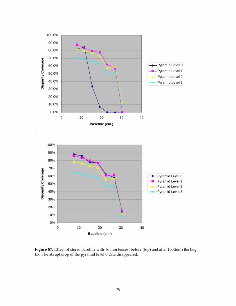
0.0%

10.0%

0.0%

100.0%

10 20

Dis

parit

y C

o

60.0%

70.0%

80.0%

90.0%ve

rage

50.0%

40.0%

3

20.0%

0 30 40

Baseline (cm.)

Pyramid Level 0Pyramid Level 1Pyramid Level 2Pyramid Level 3

10%

%

%

%

60%

1

Dis

parit

y C

o

00%

90%

80%

70%

vera

ge

Pyramid Level 0Pyramid Level 1

50%Pyramid Level 2

40 Pyramid L

30

20

0%0 10 20 30 40

Baseline (cm.)

evel 3

Figure 67. Effect of stereo baseline with 16 mm lenses: before (top) and after (bottom) the bug

x. The abrupt drop of the pyramid level 0 data disappeared.fi

79

6. Conclusion The test and validation of the JPL camera calibration and stereo vision software produced useful experimental results with in-depth analysis of stereo range errors, which are important for the error budget analysis of the rover-stereo-based instrument placement. We validated that the standard deviation σ of the stereo range disparity error for the JPL Stereo is less than 1/3 pixel (σ

1/3 pixel), so that 3σ < 1 pixel, even for very high-resolution 1024×768 stereo camera images. urther we compared the total station and laser tracker metrologies in terms of camera calibration

and stereo performances, where the laser tracker metrology is about 10 times more accurate than the total station metrology. The experimental comparison shows that the laser tracker metrology reduced the camera calibration 2-D residual error by 0.32 pixel on the average (51% reduction from 0.50 to 0.24), while it reduced the overall stereo range disparity error for a fronto-parallel surface of a rock by 0.07 pixel (30% reduction from 0.23 to 0.16). Finally two potential enhancements for instrument placement are suggested: 1) affine transform matching for sub-pixel adjustment after stereo vision and 2) combined localization using two error ellipsoids from two pairs of stereo cameras at different viewing angles. During the course of the test and validation, two software bugs were found: 1) stereo with CAHVORE and 2) maximum disparity at level 0. Thereafter, we tested the newly updated JPL Stereo software integrated into the recent release of the CLARAty vision package and verified the two bugs described above were indeed fixed.

<F

80

References A. Ansar and W. Kim, Mars Science Laboratory Technology Functional Design Document: Stereo Vision, JPL Internal Document, June 2003. Eisenman, Liebe, Maimone, Schwochert, and Willson, “Mars Exploration Rover Engineering Cameras,” SPIE Remote Sensing conference proceedings, Toulouse, France, Sept. 2001. T. Estlin, R. Volpe, I.A.D. Nesnas, D. Mutz, F. Fisher, B. Engelhardt, S. Chien, "Decision-Making in a Robotic Architecture for Autonomy." Proceedings of 6th International Symposium on Artificial Intelligence, Robotics, and Automation in Space (i-SAIRAS), Montreal Canada, June 18-21 2001.

amera Calibration including Lens Distortion, JPL Technical Reportr, D-8580, Jet ropulsion Laboratory, Pasadena, CA, 1991.

S. B. Goldberg, M.W. Maimone, L. Matthies, “Stereo Vision and Rover Navigation Software for Planetary Exploration,” IEEE Aerospace Conf., Mar. 2002. W. Kim, “Computer Vision Assisted Virtual Reality Calibration,” IEEE Trans. on Robotics and Automation, vol. 15, no. 3, pp. 450-464, June 1999. I.A.D. Nesnas, R. Volpe, T. Estlin, H. Das, R. Petras D. Mutz, "Toward Developing Reusable Software Components for Robotic Applications" Proceedings of the International Conference on Intelligent Robots and Systems (IROS), Maui Hawaii, Oct. 29 - Nov. 3 2001. D. Scharstein and R. Szeliski, “A Taxonomy and Evaluation of Dense Two-Frame Stereo Correspondence Algorithms,” Int. J. Computer Vision, vol. 47, pp.7-42, 2002.

as, T. Estlin, D. Mutz, R. Petras, H. Das, "The CLARAty Architecture for obotic Autonomy." Proceedings of the 2001 IEEE Aerospace Conference, Big Sky Montana, arch 10-17 2001.

22, no. 11, pp.1330–1334, 2000.

D. Gennery, CP

R. Volpe, I.A.D. NesnRM R. Volpe, I.A.D. Nesnas, T. Estlin, D. Mutz, R. Petras, H. Das, "CLARAty: Coupled Layer Architecture for Robotic Autonomy." JPL Technical Report D-19975, Dec 2000. Y. Xiong, L. Matthies, "Error analysis of a real-time stereo system". IEEE Conference on Computer Vision and Pattern Recognition (CVPR), San Juan, Puerto Rico, June 1997. Z. Zhang. A flexible new technique for camera calibration. IEEE TPAMI, vol.

81