The Effects of Altering Air Velocities in Operational Clean Rooms

by

Maribel VWzquez

B.S., Mechanical EngineeringCornell University, 1992

Submitted to the Department of Mechanical Engineeringin Partial Fulfillment of the Requirements for the Degree of

Master of Science in Mechanical Engineering

at the

Massachusetts Institute of Technology

June 1996

@1996 Massachusetts Institute of TechnologyAll rights reserved

Signature of A uthor ................ ................ . ... . ..................................KDepartmept of Mechanical Engineering

May 10, 1996

C e rtifie d by .................................. .. . ... .... ............................................Leon R. Glicksman

Professor of Architecture and Mechanical EngineeringThesis Supervisor

A ccepted by.............................................. ' ......... .............. .. ..........Ain A. Sonin

,,:s, rs in; 1,sT" Professor of Mechanical EngineeringOF TECHNOLOGY Chairman, Department Committee on Graduate Students

JUN 2 71996 -ng

Acknowledgments

I would like to thank some very special people who contributed to the development ofthis research and thesis. First, I thank Ruben Rathnasingham for introducing me to thewonders of spot welding hot wire anemometers. Second, I wholeheartedly thankWesley McDermott, for designing the electrical circuit which made data collectionpossible. Special thanks to my wonderful advisor, Leon Glicksman, for his support andwords of encouragement throughout this entire research, and I would like to thank PaulMcGrath, from Microsystems Technology Laboratory, for his tremendous help duringsetup and experiments. Additionally, this author thanks the National Consortium forGraduate Degrees for Minorities in Engineering and Science, Inc. (GEM) whose fundingmade graduate study possible. Lastly, I wish to especially thank Carl Loeffler whoprovided continued laughter and support during the experiments and writing of thisthesis.

Especialmente dedicado a Ilialis Hernandez, quien siempre tuvo fe en mi.

The Effects of Altering Air Velocities in Operational Clean Rooms

by

Maribel Vazquez

Submitted to the Department of Mechanical Engineeringon May 10, 1996 in partial fulfillment of the

requirements for the Degree of Master of Science inMechanical Engineering

Abstract

Experimental studies measuring velocity profiles, particle deposition and energyconsumption were performed in an operational class 10 clean room. The researchutilizes constant temperature hot wire anemometers to gather velocity profiles andanalyze turbulence intensities for 50 feet per minute(FPM), 70FPM, and 90FPM airvelocities. To measure particle deposition rates, particles were injected and retrievedwith the use of test wafers and a wafer inspection station.

The results indicate higher air velocities increase particle deposition. Additionally, thevelocity profiles indicate a homogeneously turbulent flow midway from the air source toexhaust path. However, turbulence intensities do demonstrate the dissipation of airunidirectionality close to the floor. Subsequent particle counts indicate operational cleanrooms may reduce their air velocities and remain within their current class level. Theresearch suggests a reduction from 110 OFPM to 50FPM will save a modern facility$320,000 a year in operational costs and simultaneously maintain low particle counts.

Thesis Supervisor: Leon R. Glicksman

Title: Professor of Architecture and Mechanical Engineering

Table of Contents

Chapter 11.1 Introduction

Chapter 22.12.22.32.42.52.62.7

Chapter 33.1

3.13.23.3

Chapter 44.14.2

4.34.44.5

HistoryParticlesAir FiltrationVertical Laminar FlowClean Room ConfigurationSupporting FacilityCertification

The Laminar Misnomer3.1.1 Velocity Fluctuations3.1.2 Self Preservation3.1.3 Spectral Analysis

Particle DepositionResults of Using Current ModelCritiques of Current Model

Experimental Model and SetupHot Wire Anemometry

4.2.1 Probe CalibrationHumidifier and ParticlesWafer Inspection StationConcentration Meter

Chapter 55.1 Statistical Results5.2 Turbulence Intensity5.3 Deposition Rates5.4 Analysis of Velocity Profile5.5 Conclusions5.6 Uncertainty levels

5.6.1 Probe Rake5.6.2 Probes5.6.3 TRL Facilities

5.7 Further Study

Bibliography

List of Figures and Tables

Figure 2.1- MicroelectronicsFigure 2.2- HEPA ConstructionFigure 2.3- Conventional Clean RoomFigure 2.4- Laminar Clean RoomFigure 2.5- Schematic of Typical Clean Room FacilityFigure 2.6- Construction Costs of a Clean Room FacilityFigure 2.7- Air Handling UnitFigure 2.8- Certification Levels for Clean Room Facilities

Figure 3.1- Laminar and Turbulent Velocity Profiles

Figure 4.1- Test GridFigure 4.2- Hot Wire Anemometer ProbeFigure 4.3- Yaw and Pitch Angles in Hot WiresFigure 4.4- Electrical CircuitFigure 4.4- Calibration CurvesFigure 4.5- Experimental SetupFigure 4.6- Humidifier and ParticlesFigure 4.7- WIS Wafer Output

Figure 5.1-Figure 5.2-Figure 5.3-Figure 5.4-Figure 5.5-Figure 5.6-Figure 5.7-Figure 5.8-Figure 5.9-

Statistical Properties of Velocity ProfilesSpectral AnalysisTurbulence Intensities in center test regionTurbulence Intensities in floor grille regionTurbulence Intensities in side wall regionParticle Paths for All Velocities50FPM Velocity Profile70FPM Velocity Profile90FPM Velocity Profile

Table 2.1- Particle Emission DataTable 3.1- Particle Settling RatesFlow Chart 4.1- Anemometer ConceptTable 4.1- WAS Wafer Flaw DescriptionsTable 5.1- Losses in vertical Turbulence Intensity in center regionsTable 5.2- Increases in Horizontal Turbulence Intensity in center regionsTable 5.3- Losses in Vertical Turbulence Intensity in floor grille regionsTable 5.4-Increases in Horizontal Turbulence Intensity in floor grille regionsTable 5.5- Increases in Horizontal Turbulence Intensity in side wall regionsTable 5.6- Particle Deposition DataTable 5.7- Timed eddy dissipation rates in all test regions

656768737580858687

12394763707174747677

Chapter 1

1.1- Introduction

The semiconductor and microelectronics industries have produced a wide variety

of modern products including microwaves, calculators, pagers, mobile phones, stereos,

automobiles, keyboards, and computers. However, these multibillion dollar industries,

among others, are themselves dependent upon clean rooms whose controlled

environments enable the manufacturing process. The electronics needed in today's

home appliances require a clean room environment to eliminate dust or dirt from the

product; clean rooms filter particulates from the incoming air which may cause product

failure or malfunction. By providing such environments, clean rooms have enabled the

manufacture of the numerous microelectronics and semiconductors so prevalent in the

modern world.

Unfortunately, high quality clean room facilities have been limited to large scale

corporate users because of the time and cost associated with their design and

construction. With a minimum of 6 months for design and 12 months for construction,

the cost of a fully sized clean room facility ranges between $200 million and $300

million dollars. Since a facility generally holds only 64,000 square feet of clean space,

the true cost of clean rooms ranges between $3100 and $4700 per square foot.

Shockingly, this estimate reflects solely the cost of thle edifice; the required process

tools and their installation may in some cases triple the total cost. These exorbitant

costs are forcing smaller users to embark upon joint ventures, sharing clean rooms, and

often product designs, with their competitors. 1 In addition, since the first product on the

market has traditionally enjoyed over 75% of the after market profits, clean room costs

are driving larger users to build facilities faster and faster in an attempt to produce the

first marketed product.

Since clean rooms are designed to support a manufacturing process, the facility

is classified in response to the process needs. As a result, clean room environments

require large supporting facilities, and energy consumption becomes a weighty obstacle

during operation. Over 10,000 gallons of domestic water are used monthly in a typical

clean room facility, producing a near equal amount of effluent. Typical electrical costs

range from $24,000 to $35,000 a month, and the comprehensive cost(water, electricity,

effluent etc..) of 1 cubic foot of air exhaust is approximately $25 per year. Since clean

rooms operate 24 hours a day, 7 days a week, year round, these costs compound to

reach an exorbitant amount very quickly. However, because the past two decades have

been ones of amazing growth for the clean room industry, many researchers have

failed to take a step backwards and reanalyze why clean room facilities have grown so

large, and their costs so phenomenal.

Part of the issue is that antiquated operating specifications are still currently

employed. The industry has foolhardily relied upon the original clean room model,

developed decades ago, to provide the optimal parameters for today's facilities. The

resulting overestimated specifications drive enormous facility systems and subsequent

operating costs. Because so few researchers have reexamined the clean room industry

from an operational standpoint, clean rooms have been condemned to a life of energy

inefficiency. However, the present research will identify new methods to lower clean

room energy consumption by analyzing the air handling systems and air velocity

specifications. The major goal will be to study the correlation between velocity profiles

and particle deposition rates in order to examine how lowering air velocities will

increase clean room energy efficiency and performance.

Chapter 2

2.1 History

Clean rooms produce the manufacturing environment for highly sophisticated

designs as well as the familiar home devices. Perhaps the first serious users of the

clean room were the United States military and the aerospace industry. During World

War I, controlled environments were built to eliminate the gross contamination

associated with the manufacturing areas for aircraft instruments. Heavy dust-laden air

was a frequent cause of failure in small bearings and gears used in the first aircraft

instruments. In attempting to control the area's level of contamination, the military

became the first to create what was essentially a clean room. Shortly thereafter, the

aerospace industry used the clean room concept when first exploring the idea of

satellites; miniature satellite components were assembled in contamination-free

environments in order to prevent equipment failure during orbit. Clean room technology

proved so valuable for the aerospace industry, that clean rooms are still used

extensively today in the testing of space vehicles and in the assembly of their

instrumentation.

As clean room technology evolved, it become integral in many other industries

as well. For instance, the nuclear industry currently utilizes clean rooms for the

segregation of radioactive materials, production of fuel rods, and assembly of

radioactive devices. The pharmaceutical industry recently began incorporating

contamination free manufacturing in the production of pharmaceuticals and biological

materials. In the medical profession, the amazing evolution of the operating room has

merited the designation of its own clean room class. This designation seems obvious

since the very definite need for environment control in these rooms is evident from the

meticulous care the surgeons and medical staff must undertake during "scrub-up"

procedures. Other less commonly known users of clean rooms are telecommunications

companies for cable shielding, the food processing industry for synthetic production and

packaging, and even the skiing industry for its use of fiberglass. Among the largest

users of the modern day clean room is the semi-conductor industry. Because of the

contamination related problems inherent in semi-conducting processing,

microelectronics that are now commonplace would be inconceivable without the

development of clean rooms. Modern circuitry is often so minute, that it may be

destroyed by a particle one one-hundredth the diameter of a human hair as illustrated in

Figure 2.1.

Fwua~

4-5.

Passing

a circuit

through the eye of a

FIGURE 4-5. Passing a circuit through the eye of aneedle.

Figure 2.1 - Microelectronics

2.2 Particles

The underlying theory of clean rooms is a fairly straightforward one: A clean

room is a room in which efforts have been made to control the amount of particulate

10

matter within it. However, the degrees of effort and quantity of particulate matter define

the type of clean room; a typical facility can only sustain a clean environment with less

than 1000 particles per 100 cubic foot. Particulate matter is any particle present in a

flow stream. Particles may be found in gasses, liquids and solids, as either suspended

or settled materials. Particulate matter which appears in all geometries and

configurations, and can be organic or inorganic, often has microscopic dimensions.

Virtually all tangible objects emit particles. Paper, pens, wood, clothes, and humans all

emit them. People emit extremely large quantities of particulates when performing even

minimal activity. For instance, humans emit 100,000 particles per minute merely when

standing still. Table 2.1 illustrates the quantity of particles emitted by simple activities:

Light head and arm motions 500,000 Particles per minute

Average arm motions 1,000,000 Particles per minute

Standing up from a sitting position 2,500,000 Particles per minute

Slow walk(2mph) 5,000,000 Particles per minute

Climbing stairs 10,000,000 Particles per minute

Running 30,000,000 Particles per minute

* Particles of 0.5 micron diameter or larger

Table 2.1 - Human Particle Emission Data

These particles are predominantly emitted from human skin and hair, which consist of

salt microcrystals and the protein Keratin, respectively. The skin particulates range

between 0.1 micron to 5.0 microns in diameter, while the diameters of hair particulates

range between 5.0 microns and 100 microns. Since the goal of a clean room is to

eliminate particles entirely, Table 1 indicates that clean rooms can not tolerate normal

human activity. Hence, due to the unacceptable amount of particles produced by

continued human activity, clean room personnel are required to wear specific clean

room attire, often referred to as "bunny suits". These overgarments are usually made of

Gortex and cover the arms, legs, hands, feet and head of an operator. The eyes are

protected with laboratory goggles, but the cheeks and nose are left unprotected to

facilitate breathing. However, as effective as these overgarments are, they still cannot

eliminate particle generation entirely and as a result, various other engineering

solutions are implemented in clean room particulate removal.

2.3 Air Filtration

The clean room industry considers a specific material a contaminant if it meets

two criteria: the particle must have the physical properties to cause damage and the

means to migrate to a vulnerable location. Salt and Keratin, in particular, can generate

sufficient ionic effects on semi-conductor wafers to cause extensive damage. However,

a particle's ability to migrate to vulnerable locations is dependent upon clean room

filtration and airflow. Hence, the control of airborne and transfer particles becomes the

central function of any clean room.

For the control of airborne and transfer particulates, clean rooms utilize High

Efficiency Particulate Air filters commonly known as HEPA filters. These specialized

filters remove 99.9997% of particles less than 3.0 microns in diameter from the air.

These types of filters were first developed by the Chemical Warfare Service(CWS) for

the improvement of gas masks during World War II. Later, during the development of

the first atomic bomb, the Manhattan Project utilized the CWS filter to capture

radioactive dust in order to prevent lethal radioactive doses. The scientists then

perfected the filter and was the first organization to use them for area filtration. 2

Although the numerous mechanisms enabling HEPAs to achieve high filtration

levels are complex, their construction is straightforward. Very. fine glass fiber filaments,

with diameters ranging from a millimeter to less than a fraction thereof, are formed onto

a thin pad and held into place by a resin bonding agent. The pad has an open structure

such that the interstices are no less than 100 micrometers wide and allow air passage

with a relatively low pressure drop(.3"-.5" of water typical). The glass fiber pad is then

folded around corrugated separations enabling a larger airflow with a larger filter

surface area. HEPA construction is illustrated in Figure 2.2.

Fitter Fr

mPg'.-I

Adhesive Bond

Betwenflter Pck Continuousr

and IntM I 4 ra SEho oFlat Filter

Figure 44 HEPA lter contructin.

Figure 2.2- HEPA Construction

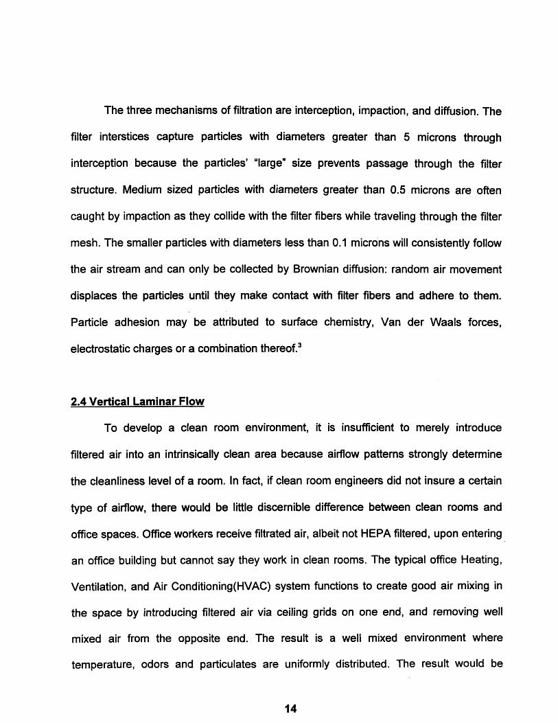
The three mechanisms of filtration are interception, impaction, and diffusion. The

filter interstices capture particles with diameters greater than 5 microns through

interception because the particles' "large" size prevents passage through the filter

structure. Medium sized particles with diameters greater than 0.5 microns are often

caught by impaction as they collide with the filter fibers while traveling through the filter

mesh. The smaller particles with diameters less than 0.1 microns will consistently follow

the air stream and can only be collected by Brownian diffusion: random air movement

displaces the particles until they make contact with filter fibers and adhere to them.

Particle adhesion may be attributed to surface chemistry, Van der Waals forces,

electrostatic charges or a combination thereof.3

2.4 Vertical Laminar Flow

To develop a clean room environment, it is insufficient to merely introduce

filtered air into an intrinsically clean area because airflow patterns strongly determine

the cleanliness level of a room. In fact, if clean room engineers did not insure a certain

type of airflow, there would be little discernible difference between clean rooms and

office spaces. Office workers receive filtrated air, albeit not HEPA filtered, upon entering

an office building but cannot say they work in clean rooms. The typical office Heating,

Ventilation, and Air Conditioning(HVAC) system functions to create good air mixing in

the space by introducing filtered air via ceiling grids on one end, and removing well

mixed air from the opposite end. The result is a well mixed environment where

temperature, odors and particulates are uniformly distributed. The result would be

14

unsuccessful as a clean room because of the particulate density and distribution. This

flow pattern displaces particles in obscure places and reintroduces them into the

environment at random locations. Because of this random displacement and uniform

mixing, air in the space would not be clean regardless of the degree of filtration.

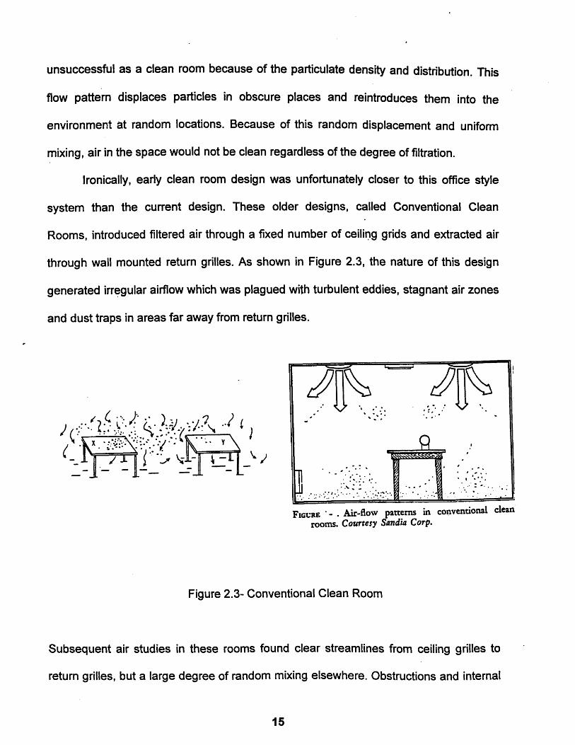
Ironically, early clean room design was unfortunately closer to this office style

system than the current design. These older designs, called Conventional Clean

Rooms, introduced filtered air through a fixed number of ceiling grids and extracted air

through wall mounted return grilles. As shown in Figure 2.3, the nature of this design

generated irregular airflow which was plagued with turbulent eddies, stagnant air zones

and dust traps in areas far away from return grilles.

2'I V2

FIGURE -" Air-flow patterns in conventional clrooms. Courtesy Sandia Corp.

Figure 2.3- Conventional Clean Room

Subsequent air studies in these rooms found clear streamlines from ceiling grilles to

return grilles, but a large degree of random mixing elsewhere. Obstructions and internal

15

ean

movements in the air path often displaced air streams to areas far away from return

grilles. As a result, cleanliness levels were determined by the time of day and amount of

workers in the area instead of by the process. In an attempt to enhance the particulate

removal of these rooms, engineers increased air velocities anticipating a greater

purging effect. However, the increased air streams resulted in air blasting problems as

stray particles on tabletops or operator coveralls were blasted from their original

locations to elsewhere in the room. In addition, the faster air streams were susceptible

to turbulent eddies far away from return grilles, which embedded particles indefinitely in

air stagnant zones. Particle counts later confirmed that larger air velocities in

conventional clean rooms contributed to increased particle retention and did not

enhance the environment.

Because conventional clean rooms lacked the desired contamination control

specifications, subsequent research in the 1960's led to the development of a new

clean room airflow pattern, called Vertical Laminar Flow(VLF). Researchers agreed that

the crucial design consideration was a greater self-cleaning capability. It appeared that

a larger airflow would be a partial solution, however, higher air flows in conventional

clean rooms were directly correlated with higher particle counts and air blast issues.

The increase in velocity would enhance particulate purging to a point, after which an

increased velocity would only stir up more dust and re-introduce it into the room. The

solution was to increase the air velocity, but introduce the air through a very large area

of diffusers. To maximize available ceiling space and simultaneously minimize velocity,

VLF utilized the entire clean room ceiling as a diffuser. HEPAs were placed in every

square inch of ceiling space and protected by grilled meshes underneath them. In this

manner large volumes of air could be introduced uniformly throughout the clean room

and their flow rate easily adjusted.

Similarly, VLF requires a large enough outlet to enable the large air volumes to

flush particles out of the clean room. This was accomplished by replacing the floor with

grated floor tiles serving as return grilles. The researchers concluded: "Laminar flow

would be produced when air was introduced into a room at a low velocity, into a space

confined on 4 sides, through an opening equal to the cross sectional area of the

confined space."4 As seen in Figure 2.4, the result was unidirectional air flow with

vertically stratified air streams to insure minimal cross contamination and little or no

transfer of energy, and particles, from one streamline to another.

FIUR -. qipen lyutindonflw -er

FICGURE - . Equipment layout in down-flow clearroom. Courtesy MAMES, Olmsted AFB, Pa.

Figure 2.4- Laminar Flow Clean Room

When the VLF prototype clean rooms displayed dramatically lower particle counts than

their conventional counterparts, Vertical Laminar Flow was fully adopted into future

clean room design.

17

2.5 Clean Room Configuration

VLF research also includes a new internal clean room configuration to control

particle and gas dispersion by physical separation. The main body of a clean room is

configured into areas designated as bays and chases with separate airflows. A bay is

the area hosting a manufacturing process while its adjacent space facilitating

equipment access is called a chase. VLF utilizes this configuration by introducing clean

air through the bays and extracting air through the chases. This configuration maintains

downward airflow flushing in the areas which sustain direct wafer contact, and upward

cleansing in the areas servicing equipment: This configuration is called Reverse Flow

and is widely implemented in larger facilities.-

2.6 Supporting Facility

Although the size of a clean room facility is measured by its square footage of

clean space, the additional facility required to support the clean room environment is

quite extensive and its cost exorbitant. Not only does each process require different

purity systems and specialized materials, but the conditioning of clean room air

demands highly effective, reliable and expensive equipment. The complexity of a clean

room facility is illustrated in Figure 2.5:

I/A

RAIISE

LENUI

Figure 2.5- Schematic of Typical Clean Room Facility

To maintain air unidirectionality and simultaneously flush out particles, clean

rooms circulate over 900,000 cubic feet per minute of clean air. Air filtration and

delivery, albeit the most important, is one of the largest and most expensive systems, in

any clean room facility. As shown in Figure 2.6, during initial construction the air

handling system alone is 18% of the cost.5

The operating costs of modern clean room facilities range between $30,000 and

$40,000 a month for electrical, domestic water, and effluent. A typical air handling

system uses $9,000-$12,000 a month of electricity, $3,000 a month for water, and

$2,700 a month for effluent.

Air must be extracted from the atmosphere, finely purified, delivered uniformly

into the clean room, and then recirculated or exhausted. Special air handling equipment

is therefore required to accomplish this crucial clean room task. Two primary types of

air handling systems develop the clean room environment: Make Up Air

Handlers(MUA), and Recirculating Air Handlers(RAH). Both air handlers work in similar

manners with a difference in air purity levels. MUAs constantly extract outside air and

condition it downstream. They provide 100% filtered air to the RAHs which combine

clean room return air with a percentage of make up air before recirculating it in back

into the clean room. A clean room facility generally uses a minimum of 25% make up air

and 75% recirculated air.

20

As shown in Figure 2.7, a Makeup Air Unit(MUA) is an assembly of components

that conditions makeup air introduced for both ventilation and replacement of exhausted

air. MUAs condition replacement air to match the existing air by heating, cooling,

humidifying/dehumidifying, and filtering incoming air. Air handling units accomplish this

conditioning through various interacting equipment such as pre-filters, heat exchangers,

de/humidifiers, and fans.

INPUTS FROM DUCT AND ROOM SENSORS

Figure Simple air handler configuration.

Figure 2.7- Air Handling Unit

The air handling process begins with the intake of outside air through louvers. Air

handler units generally rest on the roof of a facility for maximum air intake. Louvers are

also utilized for their practicality, because their sharp angle prevents large airborne

objects from flowing into the remaining air handling system. Air is first extracted from

the atmosphere and forced through a series of pre-filters. The first pre-filter is a coarse

first pass filter which removes large particles down to 200 micron diameters from the air

stream. The remaining pre-filters are a series of fine 80 micron bag filters which remove

medium sized particles (down to 5 microns in diameter) from the entering air stream.

Only after the outside air is depleted of these particles is it ready to be introduced

through HEPAs. (Since HEPAs are approximately $120 each, it is important not to

overload them with air streams containing particles larger than 5 microns.)

After exiting the pre-filters, the refined air travels through a preheat coil for

temperature conditioning. This first heat exchanger moderately adjusts the incoming air

such that equipment further downstream will not experience extreme temperatures.

Upon exiting the preheat coil, the air travels through an air-water coil cooled by chilled

water for increased temperature conditioning and perhaps dehumidification.

Dehumidification is needed in climates of high humidity whereas humidifiers are used in

low humidity regions. Dehumidification is often accomplished through cooling coils

because when moist air is cooled, it loses some of its water content through

condensation. The limit of its water capacity depends on the air temperature; the higher

the temperature the higher the humidity. If air at a particular temperature is saturated

with water vapor, a temperature reduction will reduce its water capacity forcing excess

water to condense into droplets. Unfortunately, because the amount of water removed

increases with decreasing temperature, a reheat coil is often needed to reheat the air

after it has been dehumidified. Alternative chemical dehumidification processes are

currently available, but are relatively expensive. The alternative replaces the use of

cooling coils with desiccants. Desiccants are extremely hydrophilic materials which

absorb water from air on contact. The disadvantage of this method is that after a short

time desiccants may become saturated with water and no longer absorb water at the

22

same rate. Desiccants must then be regenerated through heating to drive off absorbed

water. During that time humidity control is established through the mixing of dried air

from a dehumidifier with moist air from the inlet. The double cost associated with this

process is seldom worth the expense. Hence, the dehumidification process is often

expensive and energy inefficient, which combined with lower labor and property costs,

persuades many users to construct clean room facilities in the friendlier environment of

the South West.

The opposite process of humidification is often 100 times less expensive than

dehumidification, making it the more energy and cost efficient alternative. One of the

most popular methods of humidification is by steam spray, which is particularly ideal for

large airflows and volumes since steam sprays can supply 1700 liters an hour of

moisture into the air with only 2 pounds per square inch of pressure drop. The

drawback of using this method in clean rooms is the requirement of semi-pure spray. If

the steam spray contains any contaminants, they will be extremely well dispersed into

the subsequent air stream and very difficult to remove. The solution is to use some form

of filtered water to create the spray. However, since the water must flow through facility

piping, an extremely corrosive fluid will cause extensive damage. Fortunately, clean

room facilities utilize several thousands of gallons of semi-pure water each month,

which is then recycled and used in the humidification process. However, the use of

even this semi-corrosive fluid requires a protective glass liner for the boiler as well as

high quality stainless steel piping. Hence, although the overall cost of humidification is

much lower than that of dehumidification, it is still far from economical.

23

Lastly, one of the most important aspects of any air handling unit is its supply

fans. A fan is an air pump that creates a difference in pressure and is used to provide a

continuous air flow into the clean room facility.6 Fans produce pressure and/or flow

because their rotating impeller blades impart kinetic energy to the air by changing its

velocity. In a centrifugal fan, air enters axially then turns at right angles through the

blades and is discharged radially. The major advantages of this type of fan are its ability

to produce high pressures at relatively low speed and its external motor. With motors

located outside of the air duct, centrifugal fans have a definite advantage in the clean

room industry because motors introduce an infinite possibility of contaminants from

bearings and coils. However, since their large size often becomes a disadvantage,

centrifugal fans may often be less desirable than axial flow fans. Axial flow fans receive

and exhaust air axially. The fans' motor and blades are placed in the air stream but

develop less pressure than their centrifugal counterparts. However, in a large clean

room facility where up to five fans may be needed to drive air into a particular area, their

compact nature makes axial flow fans the fan of choice in clean room facilities.

2.7 Certification

With such extensive and costly facilities, engineers must take measures to insure

their systems are providing the desired clean room environment. Once a clean room is

designed, constructed, built and ready for use, the engineers must certify the clean

room ready for operation. Certification is the equivalent of calibrating a sophisticatedly

designed instrument; it is essential initially as well as periodically throughout the clean

room's duration. However, many clean room users do not certify their facilities as

24

precisely or as often as they should because the cost approaches several hundred

thousand dollars.

Certification verifies a facility is operating to the desired specifications by testing

all clean room parameters. Certification involves over 12 tests including those designed

to verify airflow parallelism, turbulence levels, and air uniformity. Stable vertical

streamlines should produce close to zero cross flow. Bays and chases must receive

uniform airflow, and velocity fluctuations resulting in turbulent eddies must be avoided.

Since eddies embed particles within them rather than flushing them out of the clean

room, the turbulence test is designed to single out these currents as they form due to

increased air velocity or equipment location. Certification also measures: pressurization,

temperature, relative humidity, vibration and sound level, electromagnetic

Interference(EMI) and conductivity.

Certification will also "rate" a clean room by determining its class level. Clean

rooms have traditionally been rated from Class 10,000 to Class 1 as defined by Federal

Standard 209E. Figure 2.8 illustrates the limits on each class. A class 1000 clean room,

for instance, indicates the clean space has less than 1000 particles of 0.5 micron

diameter or larger within 100 cubic feet. A class 100 clean room indicates there are less

than 100 particles within 100 cubic feet. Additionally, the current manufacture of smaller

and smaller electrical devices has prompted the new designation of Class Sub 1. This

rating certifies the facility has less than a fraction of one particle within 100 cubic feet. A

Class Sub 1 designation is extremely prestigious as less than a handful of all semi-

conductor clean rooms in the United States conform to these stringent specifications.

25

100000

10000

1000

100

10

.4

0.01 0.1 1Particle size (micrometers)

Figure 2.8- Certification Levels for Clean Room Facilities

26

M

Chapter 3

3.1 The Laminar Misnomer

This research will not treat clean

velocities combined with room height yield F

air flows with such Reynolds numbers c

inherently possess an entirely different

convenient assumptions and simplifications

rooms.

room airflows as laminar. Clean room air

leynolds numbers on the order of 105. Since

:ertainly lie in the turbulent regime, they

variety of properties, which makes the

of laminar flow inapplicable to flow in clean

Fluid turbulence in itself is a highly complex phenomenon. Turbulence may be

defined as a three dimensional, time dependent motion whose average properties may

be independent of position in the fluid. In turbulent flow there are fluctuating velocities in

three dimensions even if the mean velocity has only one or two components. In the

past, many scientists have also used the term "random" motion to describe turbulence.

In this instance, "random" does not imply that an instantaneous velocity becomes

independent of the next, but rather indicates that velocities at two points become less

closely related with increasing separation. 7

3.1.1 Velocity Fluctuations

Although there are several defining characteristics of turbulence, this research

will analyze only three: velocity fluctuations, self preservation, and spectral analysis.

Time varying velocity fluctuations are a defining characteristic of turbulent flow

distinguishing it from laminar flow. As shown in Figure 3.1, whereas laminar flows

27

sustain a steady mean value with little variation, most turbulent flows sustain

fluctuations between 0.1% and 10% of the flow's mean value:

-550

+S0.5

0.450.4

0.350.3

N (~g) a~Mr~ OQ C)Q C

Time(s) Time(s)

Laminar Flow Turbulent Flow

Figure 3.1

Not only do turbulent fluctuations vary in magnitude, but also with direction and time. In

fact, fluid turbulence develops from the growth of instabilities that lead to this chaotic

state. Due to the fluctuations in velocity, the fluid mixes rapidly and momentum is

transported quickly. The transverse velocity gradient creates high levels of shear that

generate large eddies. The larger eddies will produce smaller and smaller eddies

through inertial interaction, and in so doing, transfer energy to them. In this manner, the

eddies follow an energy cascade until the kinetic energy is dissipated through viscous

friction at the smallest eddy8. These velocity fluctuations make it advantageous for the

researcher to adopt a new definition of velocity separating velocity into Uo, the mean

velocity, and U', its fluctuation:

U= Uo+ U'. _(1)

The separation of velocity into these components permits an analysis of the fluctuation

as a function of the mean. This calculation is called the turbulence intensity and it

SerieslSeries2

provides a means to measure the level of decay in a flow field. Turbulence intensity is

defined as the root mean square of the fluctuation divided by the mean flow. The rate of

decay in a turbulent flow is critical in turbulent analysis because it provides the spatial

range in which turbulent assumptions are valid.

3.1.2 Self Preservation

Turbulent flow fields have the additional distinctive characteristic of self-

preservation. In 1940, Karman introduced the characteristic of self-preservation in

turbulent flow fields. The term "self-preserving". means that a turbulent flow pattern

retains the shape of its velocity function during decay. One indicator of self preservation

is the ability to reduce averaged flow properties by characteristic scales that depend on

a single variable. For example, if the mean velocity is given by U= U(x,y) then self

preservation may imply that there exists a length scale 8(x) and a velocity scale U,(x)

such that:

U=Usef (2)

An important consequence of this definition is that the equations of motion are reduced

by one dimension and as a result, this type of self preservation is most commonly used

in boundary layer theory. However, it is the second indicator of self-preservation, called

local similarity, which will be used in this research. The principal difference between the

two indicators is that local similarity does not lead to a reduction in the order of

governing equations. The best application is Kolmogorov's similarity of small scale

turbulent motions in high Reynolds number flows. Since clean room airflows are high

29

Reynolds number flows with small scale fluctuations, this research will utilize the

Kolmogorov microscale to identify key parameters for an accurate turbulence model.

Kolmogorov developed the theory that links the decay of large eddies into

smaller eddies and dissipation in terms of a power input per unit mass variable. This

theory suggests that small scale components of turbulence are approximately in

statistical equilibrium. In this hypothesis, turbulent motion is represented as a

superposition of periodic eddies with different lengths, time scales, and oscillations in

space. The process of energy transmission between the various scales of motion can

now be described in terms of interaction between these eddies. Kolmogorov generated

the turbulent microscale by studying the dynamics of eddies in the smallest possible

scale. He defined the time required for an eddy to dissipate into itself as the viscous

time parameter, T,, and the time required for an eddy to travel with the mean flow as

the convective time parameter, T,. The microscale was achieved by analyzing the

properties of a flow field where the viscous and convective time parameters are equal.

This condition defines the smallest possible time scale because at this instant, an eddy

would be small enough to dissipate into itself before given an opportunity to be affected

by or travel with the mean flow. By defining the time parameters as shown below,

Kolmogorov then generated the smallest scales of turbulence now known as the

Kolmogorov microscale:

Viscous Time: T= _(3)U (

Time Scale: Tk= _(4)Tk = )

Convective Time: T, = -U _(5)

Velocity Scale: Uk =6)

SV3

Length Scale: 17k -= 7)

Where L = LengthU = Velocityv = Kinematic ViscosityS= Viscous dissipation

In this microscale viscous dissipation, s , is a crucial variable as it represents the

viscous dissipation rate of the airflow. However, the nature of turbulent flow makes this

parameter very difficult to define. Kolmogorov and many other researchers spent

several years developing formulas for deriving s in various engineering flows such as

channel flow, turbulent jets, and pipe flow. This research will utilize one of the most

direct formulas derived by Kolmogorov in 1952:

2

DUS= 15V - (8)

Since the experiments produce finely detailed graphs of velocity as a function of time,

(Du/Dt) can be determined to generate a value for s.

3.1.3. Spectral Analysis

There are numerous types of turbulent flows, some of which become

extraordinarily complex. For years researchers searched for ways to analyze these very

convoluted flows until 1947 when Kolmogorov also defined the use of the spectrum

function as a way to further characterize turbulence. Spectral analysis decomposes

turbulence into elements that vary harmonically through space and time. The spectrum

function specifies a particular superposition of harmonic components with differing

frequencies or wavelengths. It gives the variation of a component's intensity with

frequency or wavelength. By using a high and low pass filter, one may see the

contributions from every part of the frequency range. The lower frequency limit is

determined by intrusion of long period fluctuations not directly associated with

turbulence. The upper frequency limit is determined by the appearance of electrical

noise at high frequencies or by a limitation in the frequency response of some electrical

equipment. As a measure of turbulent profiles and activity, Kolmogorov defined the

spectrum function that enables the researcher to examine energy versus wave number:

E(k)=KoEp/3 k-. (9)_

Where Ko = ConstantEp = Energyk = Wave Number

Since spectrum functions are widely used in turbulent studies, this research will rely

upon spectral figures to define particular turbulent flows in this clean room study. Upon

studying the velocity profiles and their spectral functions, this research will proceed to

model the airflow patterns as homogeneously turbulent flow. This type of flow was first

defined by H.K. Batchelor in 1948. Homogeneous turbulence has been considered an

idealized concept for many many years because there is no known method of exactly

realizing such a motion. However, in certain circumstances, departure from exact

32

independence of fluid properties on position can be small enough to enable a close

approximation to homogeneous turbulence. Homogeneous assumptions have been

used in the past to treat the flow in the center of a channel or pipe. The data of Comte-

Bellot (1965) showed that although such a flow is not homogeneous at low

wavenumbers, it becomes more so at higher wavenumbers corresponding to smaller

eddies. Taylor's hypothesis also supports homogeneous assumptions by stating that

the statistical properties of slowly decaying turbulence carried by a uniform flow are

identical to those that would be found by averaging these properties over a large

volume of homogeneous turbulence. 9

Currently, the closest approximation to homogeneous turbulence is described in

the flow of a uniform stream passing through an array of holes in a rigid sheet, or a

rectangular grid of bars, perpendicular to the stream. The resulting air stream maintains

the same uniform velocity with a superimposed random velocity distribution. The

random motion dies away with distance from the grid, but the rate of decay is so small

relative to the turbulent time scales that homogeneous assumptions are valid. Filtered

air is introduced into modern clean rooms in a manner remarkably similar to this

approximation. '1 HEPA filters provide an array of holes which are perpendicular to the

air stream and generate grid turbulence. They create an air stream that maintains a

uniform velocity but with points of random velocity distribution. In clean rooms, the fully

developed airflow sustains uniform turbulence in the streamwise direction and the rate

of decay can be easily measured.

Introducing the theory of turbulence and its implications enables the dynamic

incorporation of particle flow research, which has been long neglected. For instance,

33

one of the more important issues in clean room modeling is the accurate prediction of

particle deposition. Modeling turbulent clean room airflow patterns will facilitate the use

of Kolmogorov's microscale to characterize the small eddies in which particles may be

embedded. Since the micro-length scale, '9k, determines the relative size of the smallest

eddies in turbulence, the study of the eddies may be complemented with Stokes flow

analysis to determine possible particle paths and deposition rates in clean room areas.

(Stokes flow applies to the individual particles whose motion corresponds to Reynolds

numbers less than 1. )

3.2 Particle Deposition

Since the amount of particles in a clean room would be of no interest without

their deposition rates, the study of particle probability must include the study of those

factors which influence particle deposition. Particle deposition theory analyses gas-

particle flows by studying the trajectory of the particles as Stokes flow and treating the

supporting air stream as turbulent. Particle flows applicable to this research contain

small high density particles whose settling velocity is on the order of the air's root mean

squared velocity. Particles of this nature in a gas stream are easily carried by turbulent

flows and are dispersed by turbulence.

Once particles are generated and released from their source materials, they may

be carried by air currents generated by operator motion or air flow. The controlling

parameters of equipment, particle, and airflow determine whether a particle will depose

on a surface or follow the streamline around the surface. " The relative energy level

34

between a particle and a probable point of deposition controls the rate at which

particles are collected and retained on surfaces. The types of energy gradients most

important in clean rooms are electrical gradients generated by process equipment,

thermal gradients generated near worktools of increased temperature, and kinetic

gradients generated by motion. Electrical gradients may often ionize a particle and

attract it to product or equipment surfaces whereas thermal gradients can create

buoyancy effects to artificially displace particles into thermal plumes. However, kinetic

gradients are by far the most dominant because they are generated by the movement

of operators or objects as well as fans. The motion of a particle in a gas flow is

governed by gravity and the particle's interaction with the turbulent fluid surrounding it.

When analyzing gas particle flows, it is important to remember that these flows are

characterized by properties of both the particles and the turbulent gas carrying the

particles. The analysis relies on Stokes flow at low Reynolds number for the particles

and on high Reynolds number turbulent flow for the surrounding fluid.

Particles may be characterized by their density and their response time, defined

as:

T = pp Dp 2 (1)18yu

Where p = Particle Densityg. = Fluid ViscosityD,= Particle Diameter

When the particle velocity is sufficiently low(relative to the surrounding air flow) to

comply with Stokes flow(Re<l), and is dominated by viscous drag forces, the time

35

required for the particle velocity to decrease to li/e of its original value is defined as the

response time, Tp. The drag on a particle depends on the velocity as well as roughness

and surface to volume ratio of the particle itself. Although drag on particle surfaces due

to the fluid is much greater than the gravitational force exerted on the particle, near

spherical solid particles greater than 10 microns in diameter will settle quickly under

gravitational forces. Settling velocity is the velocity given a particle as a result of

gravitational forces and is defined as:

Vd=gTp. _(1 1)_

Stokes number, St, is the ratio of the response time of a particle Tp to the time scale of

the fluid, TME (time moving eulerian time scale). Using Tc, the convective time scale of

the mean flow, St indicates how ilosely particles follow the mean fluid motion.

Kolmogorov's research illustrated that particles of low inertia have velocity

characteristics which coincide with those of gas phase turbulence. Further, when the

ratio of the particle diameter to the length scale is less than 0.1, the drag on particles is

well characterized by Stokes law. Since particles in clean rooms are well within the

microscopic range fitting this criterion, this research will utilize stokes flow to analyze

particle motion.

In 1886 Stokes theory attempted to describe the forces acting on airborne

particles. The theory defines Newton's second law in the form:

m , =mg = m' g- F _(1 2)

Where m = Mass of particle = 'D3p,m'= Mass of fluid displaced by particle = 7D3pf

36

F = Force resisting particle's motiong = Acceleration of gravity

-- = Acceleration of particle

For gas particle flows with (pjpp)=.001, pressure gradient can usually be neglected, and

in most computations, the initial conditions are either zero or go to zero very quickly.

Assuming the particle is spherical, and only frictional forces are acting upon it, its

motion may be governed by Stokes' equation:

F=3nvUdp _(13)_

Substituting into Newton's equation and assuming a constant particle velocity, an

expression for the settling velocity of a particle becomes:

JV= gD 2 _(14)

However, clean room particles less than 1.0 micron in diameter will have an increased

settling speed because of their tendency to slip between air molecules with little or no

drag. For such particles, a correction factor known as the Cunningham-Stokes factor

must be applied:

vco0 , .v _(15)

Where Dc = Correction Constant = 1.172 mD,= Particle Diameter in microns

Table 3.1 illustrates particle settling rates of various sized particles with applicable

Cunningham-Stokes corrections. These figure were obtained by using latex spheres of

varying diameter in an operational clean room.

37

SETTLING RATESOF AIRBORNE PARTICLES*

Diameter of Velocity of Settlingparticles Feet per Inches Centimeters per(microns) Minute per Hour Second

0.000160.000360.00130.0020.0050.0070.0240.0950.210.380.592.49.5

21.337.959.2

352498

0.1150.2590.9361.44

* 3.605.04

17.368.4

151274425

1,7286,840

15,32027,25042,600

253,500360,000

0.0000810.000180.000660.00100.00250.00360.0120.0480.110.190.301.24.8

10.819.230.0

179253

Table 3.1- Particle Settling Rates

Defining a turbulent clean room model will support very different assumptions of

particle generation and distribution within clean rooms. When particles are introduced

into a turbulent system, the behavior of the fluid can be changed drastically depending

38

0.10.20.40.60.81.02.0.4.06.08.0

1020406080

100200400

on the particle density and size; the system has now to incorporate the dissipation due

to the particles as well as the behavior of the flow around the particles.

3.3 Results of using current model

By complying with antiquated recommendations for clean room specifications,

modern facilities may operate with air velocities as high as 110 feet per minute(FPM). 1' 2

Although this value seems high to the clean room neophyte, those in the industry for

several years have used this rigid parameter, among many others, to generate the

"Bible" of clean room specifications. Because it is often not examined carefully enough,

the original clean room prototype has developed strict paradigms in the minds of clean

room engineers. Vertical Laminar flow was so phenomenal an advancement, that few

engineers examined this research with a close eye. This has led to the common

misconception that higher air velocities produce greater self-cleansing capacities

without adverse particle or deposition effects. Although higher air velocities were proven

detrimental to conventional clean rooms, many engineers feel they are circumventing

air blast issues by adapting VLF. However, upon careful examination, one may see that

there is no magic number for air velocities in clean rooms, every facility is unique.

Ironically, although the vast majority of researchers continue to use the rigid parameters

recommended by the original VLF prototype, few are familiar with the history of these

experiments.

In 1962 Sandia's Advanced Manufacturing Development Division envisioned the

future of micro-machining. They were the first organization to begin setting design

standards and operational specifications for these highly contaminant controlled rooms

39

now called clean rooms. Sandia first constructed a horizontal laminar flow

prototype(HLF), measuring 6 feet in length, 10 feet in width, and 8 feet height, in which

to examine the various clean room parameters and generate optimal values. The study

initially analyzed airflow patterns in the prototype and then incorporated particulate

control.

The room velocity was set to 0 feet per minute and using velocity measurements,

was increased until uniform horizontal air streams could be documented. Believing

unidirectional streamlines would provide a high self-purging capacity, researchers

proceeded to alter air velocities to see the effects on particle counts. They conducted a

series of 24 hour tests in which they injected 100 micron diameter particles and

collected particle counts at the return grilles. To determine the air velocity which purged

particles most efficiently, researchers analyzed their series of collected particle counts

and selected the velocity which resulted in the displacement of the most particles at the

return. Then, based on room height and width, the prototype research proceeded to

suggest a minimum of 20 air changes per hour(ACH) was necessary to purge a

uniformly contaminated volume of air. Researchers then developed a full list of

recommended clean room specifications which include the magical 110 FPM velocity,

68 0F temperature, and 42% relative humidity.

3.4 Critiques of the Current Model

Reasonable criticisms arise when comparing Sandia's research model to modern

clean room facilities. Primarily, researchers concluded that higher air velocities yield

lower particle concentrations, but neglected to conduct further experiments to find the

40

influence of higher velocities on higher particle deposition rates. Large flow rates at high

velocities will displace a particle to the surface directly beneath it. For most clean room

facilities this means particles generated from operators will be literally pushed onto the

product. Because particle deposition is a more important factor than particle

concentration, today's engineers must consider this concept before regulating clean

room air velocities.

Sandia determined optimal air velocities by using 100 micron diameter particles

in their prototype. Perhaps this particle size was indicative of the particles emitted by

the older overgarments of the 1960's. However, today's clean room garments provide

cleanliness levels up-to 2 orders of magnitude higher by preventing the emission of

particles over 1.0 micron in diameter.13 The factors which effect large particles in the

flow stream in general do not coincide with those governing small scale particulate

motion. These large particles are insusceptible to Brownian motion, are more easily

influenced by gravitational forces and their subsequent motion is more easily effected

by drag. Gravitational forces drive large particles more rapidly towards the floor at rates

proportional to their size. Additionally, horizontal flow clean rooms entirely neglect the

gravitational effects of vertical flow clean rooms. Since gravitational effects aid in the

removal of particles, clean room air velocities could be considerably lower than

Sandia's optimum. Also, the larger surface areas of large particles makes them more

readily effected by drag. Sandia's horizontal flow clean room did not account for these

phenomena and could have quite easily over estimated their reference velocity as a

result. Moreover, particle counters are notorious for their exclusion of large particles.

Because particle counters previously measured particles by their projected area on

internal witness plates, they often recorded large particles at smaller sizes. Thus,

studying the aerodynamics of particles 100 times larger in magnitude than those

actually in the clean room, will certainly yield misleading results. Next, one must

consider the validity of the prototype's assumption of uniform particle generation and

distribution within clean rooms. In today's workplace, particles generated from operators

or equipment are localized; operators are dynamic and process equipment transient.

Increasing air velocity will indeed purge the room uniformly, .but does little to the area

where particles are concentrated. Research from the 1993 ASME Gas Particle Flows

Symposium indicates that particle concentrations and collisions peaks occur near the

viscous wall region because of thermal gradients and electrostatic effects'4 . When air

hits the wall, friction effects will redu'ce its velocity. As a result, particles will traverse

more slowly in the wall region and build up larger concentration in this area. The

particles' tendency to accumulate in this region results in particle concentrations up to

twice the order of magnitude of that in the room's center. Hence, using a uniform

particle distribution in this instance will also yield over estimated results.

Ironically, perhaps the largest factor overlooked by current researchers is

Sandia's laminar treatment of the prototype airflow. The 1993 ASME research

proceeded to suggest that concentration levels in the wall region are closely related to

the structure of air flow turbulence. As discussed earlier, the dispersion of particles in

the air flow are strongly effected by turbulent eddies generated by higher air velocities.

Faster moving eddies have been documented to embed and retain particles for up to 30

minutes, possibly displacing them into critical areas"'. By overlooking the effects of the

velocity fluctuations and subsequent turbulence intensities, Sandia oversimplified their

42

prototype model which casts doubts in their subsequent recommended optimal values.

Hence, close scrutiny of the rigid parameters imposed on most clean rooms today

illustrates the need to adjust air velocities to meet specific clean room needs rather than

set fixed values.

Over estimated velocities have resulted in gargantuan facilities which often

consume most of a community's natural resources. From a facility standpoint, the

energy costs are proportional to the cube of the air velocity16 . Higher velocities result in

larger air handler units and higher make up air requirements. Furthermore, larger

equipment and subsequent capacities result in larger redundancy specifications. From

an engineering standpoint, this can be avoided as studies from Particle Measuring

Systems have shown that filters producing a 90FPM face velocity are as efficient as

those producing 50FPM. Additionally, many engineers believe that larger air velocities

will not only flush out particles more efficiently, but also remove particles from surfaces.

However, further studies from PMS have proven that clean room airflow must travel at

speeds close to Mach 1 before they are capable of removing particles from surfaces.

Hence, there are numerous misconceptions often mandating engineers to build clean

rooms at 90FPM unnecessarily. To illustrate how clean rooms may still comply with

Federal Standard 209E and maintain unidirectional airflow at lower velocities, this

research will conduct experiments measuring the velocity profiles and subsequent

particle counts and distributions at these lower velocities.

43

Chapter 4

4.1 Experimental Model and Setup

This research will measure the velocity profiles of three separate air velocities,

50FPM, 70FPM, and 90FPM, in an operating class 10 clean room. Velocity

measurements will be taken with 8 hot wire anemometers placed on 4 different levels,

A,B,C, and D. Turbulence intensities of each level will be determine the vertical and

horizontal characteristics of each air stream. Afterwards, injected particles will measure

deposition rates with the use of test wafers and a wafer inspection station. The

anticipated results will illustrate different turbulent zones in the four levels and an

increase in particle deposition rates with higher air velocities.

This research utilizes the support facilities of MIT's Microsystems Technology

Laboratories (MTL). An 8 by 10 by 8 foot grid section of the Technology Research

Laboratory(TRL) was isolated for this research. The TRL facility is equipped with

2,000ft2 of class 10 clean room space, sustains 95% HEPA coverage and uses a

pressurized plenum arrangement for the introduction of clean air. The facility does not

implement perforated flooring but instead utilizes a large surface area of floor and side

wall return grilles.

As shown in Figure 4.1, the experimental area encloses nine HEPA filters and

one blank panel, as well as two wall mounted return grilles and one floor grille along the

area's length. Since the area lacks hard wall partitions between itself and the isleway,

visqueen along the area's perimeter simulated hard walls during experiments. The

experimental grid is divided into 15 data points and its size is limited by exhaust and

utility connections of an adjacent acid wet station and analytical equipment. The grid

44

provides the study of airflow patterns in the center, floor return, and a side wall return

regions.

Figure 4.1-Test Grid

4.2 Hot Wire Anemometry

This experiment will characterize the nature of clean room turbulent flow by

gathering data depicting the velocity profile. In order to measure fluctuating velocities at

varying spatial points, the research will utilize hot wire anemometers for their high

frequency velocity response. Since hot wires sustain frequency responses in the

kilohertz range, they are widely used for turbulence measurements in gas flows. The

underlying theory of hot wire Anemometry may be explained in very pragmatic terms.

Heat transfer theory proves that an object traveling through an air stream will lose heat

in a manner proportional to its air velocity and reach a temperature determined by the

45

rate of cooling. From this premise, it is relatively straightforward to correlate an air

stream velocity with a corresponding voltage drop in given a power supply as shown in

Flow Chart 4.1:

Flow Chart 4.1- Anemometer Concept

The hot wire anemometer probe measures the heat transfer by delivering a measurable

electrical current to a very thin variable resistance wire held by metal supports. Figure

4.1 shows the device in cross section:

46

Sensing Element

Supports

Figure 4.2- Hot Wire Anemometer Probe

Since this research is using hot wires to measure the smallest velocity fluctuation which

characterizes small scale turbulence, the sensing element(wire) must be much smaller

in length than the smallest eddy possibly measured. As a result the sensor.is very fine

measuring 1 millimeter in length, and 0.5 microns in diameter. Because the wire

changes its resistance with temperature to facilitate electrical analysis, it is important to

consider buoyancy effects near the wire which effect data by generating artificial flows.

The overheat parameter is a measure of the wire's temperature compared with that of

its ambient and is defined in the following relation:

Rw- Roa = (16)Rw

Where Ro = cold resistanceR, = wire resistance

The overheat parameter allows the researcher to consider the magnitude of free

convection effects near the wire and compensate for them. The typical value in air

streams of 80% was used in this experiment. Assuming static equilibrium, the following

energy balance is proposed:

47

dT= (W-H) =0 (17)_

Where E = Thermal energy stored in the wire = CwT,W = Electrical power = 12RwH = Heat transferred to surroundings = hA(Tw-Tf)+K(Dt/Dx)+Ea(Tw4.Tf4 )

Thermal energy is represented as a temperature dependent function of the wire's heat

capacity, Cw, and its temperature while electrical power is represented as the square of

the current multiplied by the wire resistance. Heat transferred to the surroundings

includes convection to the fluid, conduction to the supports and radiation to the

ambient. With cylindrical wires, the convection effects are measured by the heat

transfer coefficient, h, times the temperature difference, the conduction by the thermal

conductivity, K, times the temperature gradient and the radiation by the Boltzman

constant, a, times the difference of the temperatures to the fourth power.

By the nature of this instrument, it is important that probe casings and body are

slender enough to prevent interruptions in the flow around the wire, but also rigid

enough to prevent wire vibration. In doing so, hot wires require prong supports which

are more massive than the wire and unfortunately leads to increasing conduction

effects with heat loss from the wire to the prongs. However, keeping the wire's aspect

ratio, length over diameter, at approximately 200 will limit these effects"7 . Radiation

effects become important when there is a large temperature difference between the

wire and the ambient. Because the effects follow as the temperature difference to the

fourth, heat transfer effects may be significant. However, radiation effects are safely

assumed to be less than 10% of the total heat transfer in normal applications. Thus,

48

with hot wire anemometry, forced convection associated with the heated wire can cause

significant vertical movement of its adjacent fluid. The severity of buoyancy effects are

indicated through the flow's Grashof number, Gr. Previous research in hot wire

anemometry suggests that if the flow's product of Grashof number and Reynolds

number is less than 10000, it will generate insignificant free convection effects near the

wire. However, recent research from Leinhard at MIT"' indicates a less stringent criteria

which states that flows with Grashof numbers less than their corresponding Reynolds

number to the third power, have negligible free convection effects. Hence, the minimum

velocity reliably measured with hot wire anemometry is that which is equal to the free

convection created by the wire. In this case, free convection is limited to velocities

under 0.1m/s. Since this research will operate within these constraints, free convection

effects near the wire will be neglected.

One crucial heat transfer consideration in hot wire anemometry is the effect of

the wire's yaw and pitch angle. As shown in figure 4.3, a three dimensional flow will

enable velocity measurements at different angles in the three planes. The yaw is the

angle incident to the wire in the plane parallel to the supports, while pitch angles are

measured in the plane perpendicular to the wire and supports. Altering yaw or pitch

angles will change the velocity vector incident upon the wire and in so doing effect the

heat transfer. Since the device will primarily measure the velocity component

perpendicular to the wire, it will return lower values for yawed velocities because it can

only measure the projection of the velocity vector in this plane. At first glance, pitched

velocities would not seem to effect the heat transfer since the vector is always

perpendicular to the sensing element. However, the 1993 ASME Symposium on

49

Thermal Anemometry indicates that placing supports perpendicular to a mean flow may

causes wakes near the wire resulting in more heat loss to supports and a higher output

from the probes19. Although some may argue that pitch effects are minimal, velocity

readings may be easily adjusted using corrections called K factors. Yawed velocities

produce first order effects and are corrected by K1 factors while pitched velocities

produce second order effects and are corrected by K2 factors. Both factors depend on

individual angles and velocities however yaw angles require more stringent corrections

on the order of 20% while pitch angles require a correction of only 5%. Because these

experiments utilize the devices configured at a 900 pitch and 0* yaw, the output voltages

will be corrected by roughly 5%.

YAW AND PITCH RESPONSE

Yaw

yaw mIdfteb Aisle CQm C.M&edbfabe

Figure 4.3- Yaw and Pitch Angles in Hot Wires

Proceeding with the assumption that convection effects dominate, and device

configurations do not significantly alter the energy balance, the static equilibrium

equation reduces to the following:

50

12R,= hA(Tw-T,) _(18)

These relations establish how heating current is used as a measure of velocity. Hot wire

anemometers determine a flow's velocity through the circuit's corresponding output

voltage. A Wheatstone bridge and high gain servo amplifier are used to drive this

research's devices. The circuit is initially balanced with the "cold" wire but designed to

react quickly as velocity fluctuations alter the wire's resistivity and cause voltage

imbalances in the circuit. W, the joule heating in this circuit, can now be more

accurately represented as:

W = 12R, = E, 2 = R,(R,-Ra)(C 5+C64U) (19)_

WhereE, = VoltageCs,C6 = Constants

Since the experiments must measure accurate velocity fluctuations, numerous electrical

stages were needed to boost the electrical signal. Unfortunately, Dantec Technologies

has documented that use of 12 bit A/D converters in most hot wire anemometer

applications will yield noise levels equivalent to a 2% turbulence level.20. Since this

experiment anticipates velocity fluctuations within 1.0% of the free stream velocity,

several control measures must be implemented. Because air velocities in clean rooms

are on the order of 0.5 m/s, velocity fluctuations at .05m/s border the minuscule and a

series of high gain Operational Amplifiers(Op-Amps) are essential in the anemometer

circuitry. As shown in Figure 4.3, the experiments utilize Constant Temperature

Anemometers(CTA) by supplying a constant voltage sustaining a constant hot wire

temperature.

Figure 4.4 - Electrical Circuit

The required resolution and magnification of the output signal are accomplished

through various Op-Amp stages within the Servo Amplifier: Input and Output(I/O)

Buffers, Multipliers and Scalers. Each probe retains its own corresponding electrical

circuit consisting of 10 resistors, 6 Op-Amps, and 2 potentiometers. One potentiometer

serves as an input bias while the other is utilized as an output bias. These variable

resistors must regulate the input and output voltages corresponding to a specific

probe's resistivity. The bridge formed by these potentiometers essentially functions as a

control system for probe resistance, maintaining the resistance in response to changes

in convective cooling by varying the voltage across the probe. The time varying voltage

52

CONSTANT TEMPERATURE MODEi

1i

I

I

i

1

signal associated with maintaining the wire resistance at the level determined by the

overheat ratio constitutes the primary output of the bridge amplifier system.

Although the circuit will balance itself extremely quickly, because the control

system is defined by a differential equation, the wire's thermal lag will yield a finite

velocity response of:

Y(f) = Y(t) edt _(20)

By dividing the output function by the input, the system transfer function may be

determined as:

Kc:H(f)= 21)

1+ jWTar

TWhere Tct = Frequency Response: Tc, =

2aS'RwS' = Amplifier gaina = Overheat parameter

The time constant, Tc, defines the frequency response of the system which will be on

the order of 25Khz for this experiment. As a result, a sampling rate of 100kHz was used

in an attempt to characterize the smallest time scales. One important consideration is

that the spatial resolution of the response be proportional to the sensor dimensions.

The circuit cannot resolve scales smaller than the wire diameter and will hence be

limited in its frequency range.

4.2.1 Probe Calibration

Despite extensive work, there exists no universal expression to describe the heat

transfer from hot wires. It is for this reason that all actual measurements require direct

anemometer calibration. Initial and frequent calibration is essential with every hot wire

usage because it enables the researcher to produce reliable data from the conversion

of experimental measurements. Since high level fluctuations often influence the

measured voltage across hot wires, it is advantageous to calibrate probes in low

turbulent flows. As a result, this experiment's probes were dynamically calibrated in the

velocity range of their anticipated usage using a low turbulence wind tunnel. Given the

nature of clean room air velocities, it would be advantageous to calibrate the probes at

the smallest velocity possible. Although clean room crossflows may approach 0.2m/s,

the wind tunnel motor could overheat-at velocities lower than .28 m/s, forcing the use of

a 0.3m/s-0.8m/s range instead. By varying the wind tunnel airspeed, known air

velocities are directly correlated with output voltages. King's Law results in voltage-

velocity curves shown in Figures 4.3(a)-(h):

V2 = A+Bu" _(22)

Where A,B = Constant

n = Velocity ExponentFigure 4.3(a) - Calibration curve for probe 13.8

3.7 ...... ........ -... ............. .... ...

3.6 7----. --............

3.4 ........ ...

3.20 0.2 0.4 0.6 0.8

Velocity

Figure 4.3(b) - Calibration curve for probe 22.8

2.6

&2.4

> 2.2 . ... ...... ........ .........

2 ........ ........................... -

1.80 0.2 0.4 0.6 0.8 1

Velocity

Figure 4.3(c) - Calibration curve for probe 3

3.9

3.8

3.7CO

> 3.6

3.5

3.4

0

Figure 4.3(d)Z.8

2.7

02.6

> 2.5

2.4

2.30.2 0.4 0.6 0.8 1

Velocity

- Calibration curve for probe 4

0 0.2 0.4 0.6 0.8Velocity

Figure 4.3(e) - Calibration curve for probe 5 Figure 4.3(f) - Calibration curve for probe 6

0 0.2 0.4 0.6 0.8

Figure^ ^"

0a

0

Velocity

4.3(g) - Calibration curve for probe 7

0 0.2 0.4 0.6 0.8Velocity

FigureA f

4.6

0 4.4

4.2

Velocity4.3(h) - Calibration curve for probe 8

0 0.2 0.4Velocity

0.6 0.8

55

3.6

0 3.5

> 3.4

3.3

3.2

J. It J

33 1

J.7f

4.8

I

Further research on King's law has illustrated the velocity exponent increases with

lower velocities. Hence, although recent papers have suggested n = 0.45 as the better

exponent, this research used the standard n = 0.5. Although this relation is among the

most standard for hot wire calibration, it retains some inherent impracticalities. For

instance, the constants A and B must be determined given input voltages and

corresponding velocities. However, one cannot easily set zero voltage as a means to

determine A because natural convection effects make it nearly impossible to obtain a

true zero velocity. Further, the uncertainty due to natural convection is neither evident in

velocity nor voltage. Additionally, a linear least squares fit is inapplicable because

King's law is not linear and a higher order polynomial lends itself to further errors.

These may be sources of error in the data.

As hot wires respond to convective cooling with a fluctuation in voltage, they

transmit this output to a data acquisition unit. A Metrabyte DAS16G Internal Analog to

Digital(A/D) converter and an Intel 486SX CPU was used to gather data throughout this

research. The A/D board can receive up to 16 channels of unipolar signals. It receives

signals between +OV and -10V but represents each voltage as number between 0-

4095, where 1 bit represents approximately 2.25 milivolts. A short cable connector

attaches the A/D board to a smaller auxiliary board where screw terminal connections

receive output voltages from the individual circuits and transmit them to the A/D board

for data collection; the signal to noise ratio was measured to be 6:1. Figure 4.5

illustrates the experimental setup:

56

Hot Wire Anemometers

Wire Vertical

Probe Rake

.75'

Figure 4.5- Experimental Setup

Since hot wire anemometers are delicate apparatuses which may be easily

destroyed by excess vibration or direct contact, they are mounted onto a probe rake for

protection during experiments. The probe rake is a steel L-shaped pole 7 feet in height

containing one millimeter diameter holes spaced one half inch apart on its sides. The

need for adjustable probe locations contributed to the rake's distinctive geometry as

these perforations allow probe locations on any level. The hot-wire anemometer probes

are placed 2 on each level at 1ft, 3ft, 5ft, and 7ft elevations. In order to measure vertical

velocities, odd numbered probes are aligned such that their wires are horizontal,

perpendicular to the probe rake. These wires are also perpendicular to the 10 foot

length of the room, see figure 4.1 The wires of the even numbered probe are aligned

57

I..i 6 !

vertically, that is parallel to the probe rake in order to measure crossflow velocities. The

2 foot spacing was chosen corresponding to the length of the HEPA filter. This research

anticipates that clean room flow fields will change with distance from the air source in

sections equal to the HEPA's cross dimension.

Probes in the same plane sit perpendicular to each other to best facilitate two

dimensional velocity measurements as well as prevent contact between probes. The

probe rake containing all 8 hot wire anemometers is moved along the various grid

points to determine a velocity profile. The probe heights were chosen such that different

probes will yield velocity profiles corresponding to different flow fields. Probe 7 and

Probe 8 are.placed at the highest level, Level A, located only 8 inches below the HEPA.

Due to the eddies generated by HEPAs, the velocity profiles from these probes are

anticipated to be homogeneously turbulent. Probe 5 and probe 6, are located 3 feet

from the ceiling, on Level B, and should detect a decaying but unidirectional flow field.

Likewise, probe 3 and probe 4 are located on Level C, 5 feet from the ceiling, and

should depict a deteriorating flow field with increasing crossflow. Probe 1 and probe 2

are in Level A, placed 7 feet from the ceiling(1 foot from the floor) in a region where

crossflow currents should be very strong and unidirectionality dissipated.

By moving the probe rake along the grid points, the effect of each flow pattern

near the center, floor exhaust and side wall exhaust are shown. Before each test, the

air flow is left undisturbed for 5 minutes to achieve steady state. Afterwards, velocity

readings are taken for one minute at a 100kHz sampling rate. Probes and circuitry are

tested periodically before and after each test. The results will depict velocity profiles of

three clean room air velocities: 50 FPM, 70FPM, and 90FPM.

4.3 Humidifier and Particles

Upon measuring airflow patterns, the experiment proceeds to study how each

pattern effects airborne particulates. To accomplish this, particles are injected into the

experimental area and their deposition monitored. For more accurate results, particles

injected into the experimental area should closely resemble the types of particles

emitted by clean room personnel during normal operation. However, with the diversity

of particles possible, it is impossible to determine what size particles are emitted where.

To make this process proceed more smoothly, the industry has adopted the practice of

using spherical particles when studying the dynamics of clean room particulates. These

particles are injected in a manner consistent with clean room certification specifications.

(Although the particles are not intended to challenge the HEPA filters themselves, the

procedure is still a useful one for its particle injection techniques.) This experiment

utilizes 0.499 micron diameter particles made of polystyrene and certified by the

National Institute of Standards and Technology. One 15 milliliter vile of particles, at

0.1% solid, is combined with 1000 ml of water to generate the particulate stream. This

mixture is placed into a standard non heating, non purifying humidifier and displaced

into the clean room at a 450 angle from the horizontal at a rate of .075 milliliters per

second in the form of a vaporous spray. This rate was verified by calibrating the

humidifier and comparing it to the manufacturer's specifications. The humidifier unit was

filled to capacity, weighed, and then operated in four 2 minute intervals. After each test,

the unit's weight was compared to its initial value which resulted in the corresponding

flow rate. The four test trials demonstrated a consistent pattern with a standard

deviation of 1.73%. The humidifier is then positioned in each of the three test regions,

center, floor return and sidewall, return for each velocity. The humidifier mist introduces

particles for 90 seconds and is then shut down for 120 seconds to allow particle settling

and deposition as well as exit through return grilles. This procedure introduces 7.4x10 4

particles into the experimental area with each particle spray. Three perimeter wafers

permit deposition analysis afterwards.

Based on visual observation, the humidifier's dispersion rate of .075ml/s is able

to produce a flow plume that is 30 inches in diameter when passing through the plane

containing the wafers. In order to study the deposition of particles at different air

velocities, three clean 6 inch wafers are placed around the humidifier's perimeter 20

inches away from the nozzle and 20 inches apart from each other as shown in Figure

4.6:

F

HEPAs

Test

96"

20"

7

7

60

Figure 4.6(a)- Humidifier and Wafer Location

c/iý.

ne

20"

I

I

I/

[177277IHumLIlder

30"

Figure 4.6(b)- Plan View of Test Wafers and Humidifier

The wafer surface area accounts for only 1/25 of the plume area but should catch

significant particles. This procedure is performed at the center of the experimental

space, near a side wall grille, and near a floor grille for the three identified velocity

profiles. After particle injection, the test wafers are carefully removed with nitrogen

vacuum wands, so as not to artificially contaminate their surfaces, and placed into an

inspection station.

~·

irr

4.4 Wafer Inspection Station

Once particles depose onto a wafer surface, a Wafer Inspection Station(WIS)

can produce a particle count, size and distribution on each wafer, see Figure 4.7. Since

particles are three dimensional objects, they can be described by their volume, their

cross sectional area, their largest dimension or an arbitrary dimension advantageous for

the research. The choice is a function of the product the particle will contaminate, and

as a result, various methods are used to measure quantity of matter. For instance, in

the semi-conductor industry the particle's largest dimension is of interest because of the

sensitivity of the wafer. However, in the bio-pharmaceutical industry, the nature of

bacteria and other biological products, as well as the strong effect of electrostatics on

these materials, require monitoring of a particle's projected area. The Wafer Inspection

Station(WIS-100/150) will describe this experiment's particulate matter in terms of its

size and distribution on the test wafer. The WIS-100/150 uses a spot laser scanner to

sweep a beam of light .003 inches in diameter across the wafer surface.21 Channel

detectors collect and scatter light from the wafer surface to produce frequency and

amplitude distortions in light. Since the amplitude is proportional to the size of the

wafer's surface flaw, particle size and distribution are easy displayed within 1%

accuracy. Table 4.1 shows the flaw descriptions.

62

:E=LA'- OFF

..O0

O

OC

Evn: E = GN

FLAWNUMBER DEFECT (THRESHOLD UTILIZED).... ... .... ... .. ....... ,....,,.... ... ..... ........ .........

234

S

6

7

8

9

1011

12

13

141516

Haze (T-1).Small pits and particulates (0.3 to 2 microns) (T-2)..Larger pits and particulates (2 to 20 microns) (T-3).Cumulative sum of 2,3.A.C. and G defects. Totalizatiotnof particulates.Scratch count. 1,2, and 3 defects in a minimum of fouradjacent pixels are converted to 5's and analyzed fo!.scratches.Area defects.Light orange peel. partially polished out saw martsgenerally low level and frequency (T-4).Distortion with abrasion such as an unpolished out sat.,mark (T-4 and T-3).Distortion defects of higher frequency such as smaldimples, grooves, and mounds (T-5).(A) Large particulates (T-5 and T-3).(B) Heavy orange peel and related defects (T-5 and

T-4.)(C) Severe dirt, abrasions, or film (T-5, T-4. and

T-3).(G) Number of edge types not resolved. Also very

large defects (T-7).Not currently used.Not currently used.Not currently used.

Table 4.1- Wafer Flaw Descriptions

--:E =-::R MA[?i4 MEN'"

Figure 4.7 - Wafer Output

4.5 Concentration meter

Before placing clean test wafers in the experimental area, a PMS-126

concentration meter will verify the quantity of pre-existing particles. This safety

precution reflected zero pre-existing particles in the clean room which indicates the

majority of particles on the test wafers are the experimentally injected ones. The PMS-

126 concentration meter utilizes a small vacuum wand to extract air from a desired area

and count the airborne particulate contaminants within it. The concentration meter

deciphers particle size and sorts them into different concentration categories. The PMS-

126 is limited in that it may detect particles as small as 0.1 microns in diameter, but

cannot distinguish those greater than 5.0 microns. However, since particles less than 1

micron in diameter are the only variety in clean room facilities, this particle counter was

sufficient for this research.

64

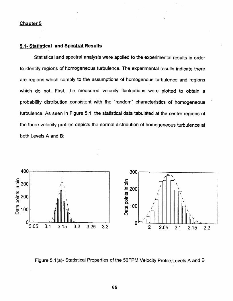
Chapter 5

5.1- Statistical and Spectral Results

Statistical and spectral analysis were applied to the experimental results in order

to identify regions of homogeneous turbulence. The experimental results indicate there

are regions which comply to the assumptions of homogenous turbulence and regions

which do not. Fiirst, the measured velocity fluctuations were plotted to obtain a

probability distribution consistent with the "random" characteristics of homogeneous

turbulence. As seen in Figure 5.1, the statistical data tabulated at the center regions of

the three velocity profiles depicts the normal distribution of homogeneous turbulence at

both Levels A and B:

3.05 3.1 3.15 3.2 3.25 3.3

300r

.S 200-,

z100

02 2.05 2.1 2.15 2.2

Figure 5.1 l(a)- Statistical Properties of the 50FPM Velocity Profile;Levels A and B

400

5 300u,

.c 200oa

0a

0

I11 \

3.15 3.2 3.25 3.3 3.35

400

"5 300C

200

(a*6 100

02 2.05 2.1 2.15 2.2

Figure 5.1(b)- Statistical Properties of the 70FPM Velocity Profile;Levels A and B

2.9 2.95 3 3.05 3.1

400

0 300C

.• 200a

o16 100

03.9 3.95 4 4.05 4.1

Figure 5.1(c)- Statistical Properties of the 90FPM Velocity Profile; Levels A and B

66

,~ -~ ,.~

JUU

cc 1000

0

/ -

\

II

/d l"nm-

bUU

.5 400

0a

AIA

v

This data is the first step in demonstrating the existence homogenous turbulence in the

three velocity profiles up to level B, half way from the ceiling to the return. Below this

level however, the airflow dissipates into other forms of turbulence which cannot be

easily categorized by this research.

Figure 5.2 further characterizes the turbulent flow through the use of spectral

analysis. One distinctive characteristic of homogeneity is the so called 5/3 law. When

Kolmogorov defined the spectrum function as a means to characterize turbulent flows,

he paid particular attention to the most ideal case of homogeneous turbulence. By

correlating the self-preserving characteristics and the generated mesh turbulence,

Kolmogorov concluded that the spectral functions of homogeneous flows will display a

decreasing slope of 5/3 in the frequencies corresponding to the flow's smallest turbulent

time scale. The data gathered at the center test region illustrated high noise levels in

the lower wave number ranges. As a result, the curve's slope was determined using the

signal to noise ratio of 6:1. Only the data points a fraction 1/6 above and below the

mean value were used to determine the slope of the line. Within the experimental

section of the clean room, the slope of the spectral graph was identified as 5/3 with

corresponding frequencies beteweenl0 2and 105 Hz.

67

- 2

IV

10- 3

10-4

10

10- 6

10-s 10. 10- 10- 2

Wave Number

Figure 5.2 - Spectral Analysis

During these experiments, the center test regions of all three air velocities exhibited

homogenous turbulence up to Level B, midpath. After this level, however, crossflow

velocities were too strong to maintain unidirectionality.

5.2- Turbulence Intensities

Since analysis of turbulent intensities helps identify regions of unidirectionality,

turbulence intensity plots of the vertical and horizontal velocity components were

generated for the three test regions. Figures 5.3(a)-(c) depict the averaged vertical and

horizontal turbulence intensities in the center regions of the 50FPM, 70FPM,and 90FPM

velocity profiles. The brackets indicate the standard deviations which were +/- 5% and

+/-9% in the vertical and horizontal intensities respectively.

Figure 5.3(a)-Turbulence Intensities in the 50FPM Center Test Region

68

6

4

c3

0

0

a) - -Vertical

0-A.... Horizontal

1 3 5 7

Feet from HEPAs

Figure 5.3(b)-Turbulence Intensities in the 70FPM Center Test Region

Figure 5.3(c)-Turbulence Intensities in the 90FPM Center Test Region

The 50 FPM vertical turbulence intensity curve indicates a rapidly decreasing intensity

towards the floor. Although the velocity reading 3 feet from the HEPA(Level B) indicates

69

4.5

4-3.5

S3-2.5S2

S1.51-

0.5;n

- :::: :::::: -ii~,, :i::::::iil:,,,:,i:iiiiiii:i

- ~ '::'~ i:ii:(li'il':.ii~iiii

': :: . * i- :':::::: ::-*: : ·:: ··

1 3 5 7

Feet from HEPAs

43.5

'o 3

- 2.5

22 1.5

0.5

0

- -- VerticalA.... .. Horizontal

Feet from HEPAs

--- -VerticalS- --- --- Horizontal

T

Feet from HEPAs

a loss of 43% in turbulence intensity, the reading 7 feet from the HEPA(Level D)

demonstrates an 87% loss. In the case of 70 FPM, the velocity reading 3 feet from the

HEPA(Level B) indicates a loss of 41%, and an 85% loss by the reading 7 feet from the

HEPA(Level D). Similarly, in the 90FPM case, the velocity reading 3 feet from the

HEPA(Level B) depicts a 39% loss in turbulence intensity, and an 82% loss by the

reading 7 feet from the HEPA(Level D). The respective losses in vertical turbulence

intensity are summarized in Table 5.1:

Velocity 1 Ft from HEPA 3 Ft from HEPA 5 Ft from HEPA 7 Ft from HEPA(Level A) (level B) (Level C) (Level D)

50 FPM 0% 44% 78% 87%

70 FPM 0% 41% 77% 85%

90 FPM 0% 39% 74% 82%

Table 5.1- Losses in Vertical Turbulence Intensity in center regions

These observations have profound results because with a significant decrease in

turbulence intensity, initial modeling of homogeneous turbulent flow may become

inapplicable. Previous research from Batchelor indicates that when a turbulent flow

loses more than 50% of its initial turbulence intensity within the length of the flow path,

it may or may not retain similar flow patterns22 . With this guideline, the research may

safely assume homogeneous turbulent flow exists slightly below level B, approximately

4 feet from the HEPAs, but not below.

As seen in the complementing horizontal turbulence intensities, the vertical

turbulence intensity is not "lost", but rather transferred into crossflow 23velocities. The

70

horizontal intensities of the 50FPM velocity illustrate a 59% increase 5 feet from the

HEPA(Level C). Similarly the 70FPM and 90FPM velocities demonstrate a 61% and

62% increase, respectively. Table 5.2 illustrates the data below.

Velocity 1 Ft from HEPA 3 Ft from HEPA 5 Ft from HEPA 7 Ft from HEPA(Level A) (level B) (Level C) (Level D)

50 FPM 0% 11% 59% 74%

70 FPM 0% 9% 61% 71%

90 FPM 0% 8% 62% 70%

Table 5.2-Increases in Horizontal Turbulence Intensity in center regions

Unfortunately, the experimental apparatus could not capture all of the turbulence

intensity data in the two dimensional plane. As a result, the losses of vertical turbulence

intensities do not correspond exactly with the increases in the horizontal intensities.

However, the gathered data still indicates a departure from vertical homogeneous

turbulent flow towards an increasing horizontal crossflow near the floor. Since return

grilles provide negative pressures, much of the neighboring air is drawn away from the

vertical flow and transferred into crossflow. In this manner, return grilles not directly

underneath an air stream may create a secondary flow which alters the mean velocities

as well as causes the measured losses/increases in turbulence intensities.

The turbulence intensity plots of air streams directly above floor grilles illustrate a

more unidirectional path. Figures 5.4(a)-(c) indicate the downflow velocity retains a

large part of its initial turbulence intensity as far away as 5 feet from the HEPA

Figure 5.4(a)-Turbulence Intensities in the 50FPM floor grille region

Figure 5.4(b)- Turbulence Intensities in the 70 FPM floor grille region

72

.i ..i....:..:'' :.-i:i • " " " .... ... ........ ...... • ::

-• ii• , •! il i i.'i

• ...,.i : .• . .. .... .: .. ..•::i : ..:.::.:::i::::: i-.:.": ': ":. .I';2.5:':':' - -*--- VerticaU -A --Horizontal::i:::i:::;::::

1+ -

3.5

' 30

2.5-

S2-.e 1.5

0.51

0*

1 3 5 7

Feet from HEPAs

I

.... A .. Horizntal

305

4

3.532.5

S2

1 1.5-.0

0.5 4

0

---- Vertical

-- -..... -Horizontal

1 3 5 7

Feet From HEPAs

Figure 5.4(c)- Turbulence Intensities in the 90FPM floor grille region

These results reflect homogeneous turbulence to a level slightly below Level C,

approximately 6 feet from the HEPAs. These results, however, are anticipated because

VLF has previously illustrated that perforated floor grilles directly beneath an airflow aid

in maintaining the flow's unidirectionality. However, by averaging the instantaneous

anemometer readings to obtain experimental mean velocities, this research has

nonetheless confirmed that there is little difference between the unidirectionality of a 90

FPM profile and a 50 FPM profile in regions near floor grilles. Tables 5.3 and 5.4

illustrate the data.

73

rA'-

.--

`

*r

305

Velocity 1 Ft from HEPA 3 Ft from HEPA 5 Ft from HEPA 7 Ft from HEPA(Level A) (level B) (Level C) (Level D)

50 FPM 0% 10% 21% 30%

70 FPM 0% 8% 17% 27%

90 FPM 0% 5% 14% 25%

Table 5.3- Losses in Vertical Mean Velocities in floor grille regions

Velocity 1 Ft from HEPA 3 Ft from HEPA 5 Ft from HEPA 7 Ft from HEPA(Level A) (level B) (Level C) (Level D)

50 FPM 0% 13% 25% 40%

70 FPM 0% 9% 21% 36%90 FPM 0% 7% 17% 31%

Table 5.4- Increases in Horizontal Mean Velocities in floor grille regions

Figures 5.5(a)-(c) indicate the turbulence intensities near side wall returns have a

different pattern. The vertical turbulence intensity decreases steadily until shortly after

Level B, 3 ft from the HEPAs, where the effects of crossflow cause a sudden increase

in turbulence intensity.

74

Figure 5.5(a)-Turbulence intensities in the 50FPM side wall region

Figure 5.5(b)- Turbulence Intensities in the 70FPM side wall region

r .I**

~ - -.--*V rtca

2-E" • .....i'.ii......:: : : -:iL:--:.!::.!:::-:::::i.:i:- ii-• i:·-i:iii~i• ::: Hi:ii•:i:·::: · ii~i!• •i-i!i: ~ !•• • i• ..::::"•:,? i)'•:::!:.!!:::i!:•?> • :• ::::'•ii? :ii,!ii:: !: ; •:-::'::! ' )i ?::.:i ; •:::?!• !:!!!!!?! !• ' :!iii: .i!'•!i'::~i~·` : :l- i' ,!: i !!'!• i i:: ':)) ; •:•+C:it: :"I:: ! Iiiii!)i!•!)i ~i

.• -;:.:...::ii:::::". " :-:-!!•::)•):)):•:•:••2:•ii::ii:::•J•!=:i~!•~i);!i~•)f:)•--.-.:•::•:::.))•.,=g!••::•:••ii:Ni•,•i• ii!!!i:!! i iiii I

ii i• ::.-i:.::-.::!':•:•i•::!!-." .' • ..:- !:.•::?-:::•i:•:!•:::::••:•i::• ! : • : i "i :•!i• i:!• •! • •:!•• •::• ! ! !) ! !•) !•:i

IU

9-U) 8c 7-

6 -S5S4-S3-

0

-- - Vertical

--.... l-A ... -Horizontal

1 3 5 7Feet from HEPA

a0

7

Z 6

5

a42 4

e2

1

0

- ---- Vertical.-.. - -- Horizontal

Feet from HEPA

0 -.

Feet from HEPA

Figure 5.5(c)- Turbulence Intensities in the 90FPM side wall region

This phenomenon is a function of the dimensions and location of the sidewall

grille. The grille measures 1 foot by 1 foot and is mounted 1 foot above the clean room

floor. Because particles will often impact the grille mesh at odd angles, they may be

pushed back into an eddy several times before being extracted through the grille.

Particles re-displaced into eddies may be pulled towards the floor by gravitational

effects where they can swirl indefinitely before extracted through floor grilles. This

generates larger crossflow velocities and increases turbulence intensity as illustrated in

Table 5.5.

3 5

.etfrmHE-.E ;:: 4- --- Vertical(0 * - -- A- -- Hori onta

4 iiii:::~~

7

6r t

4-1c 3-

2-

i

0

1 3 5 7

Feet from HEPAs

iaole b.b- Increases in Horizontal Turbulence Intensity in sidewall regions76

V ertca.... A... Ho~zn

Initially, the sidewall results seem misleading. How can a flow lose turbulence intensity

and then regain it so quickly without additional energy? The answer to this question lies

in the increase of horizontal mean velocities, turbulence intensity and in the location of

the probes. Because sidewall grilles extract flows utilizing so large a surface area, the

horizontal mean velocity increases so quickly that close to the sidewall there is often

reversed flow during air extraction. Unfortunately, the anemometers used during these

experiments are incapable of measuring reverse flows and consequently, data seen

past level C, 5 feet from the HEPAs, is inconclusive.

5.3- Particle Deposition Rates

Characterizing turbulent velocity profiles permits the analysis of their effects on

particle deposition. In the three test regions of each velocity, the following particle

deposition rates were observed:

Air Velocity Particles on Wafers Particles on Wafers Particles on Wafers

(Feet Per Minute) (Center) (Floor Grille) (Wall Grille)

50 FPM 45 54 120

70 FPM 51 238 407

90 FPM 56 316 546

Table 5.6- Particle Deposition Data

77

The data implies that clean rooms operating at higher air velocities will sustain

increased deposition rates. This phenomenon may be attributed to air blast issues

associated with higher velocities. When a particle is introduced into a clean room in the

form of a jet, the flow pattern of that particle is heavily dependent on the velocity of the

pre-existing air stream. A particle is immediately displaced by the existing air velocity

and is moved towards the floor by gravity and the flow's inertia. Further, the flow's

turbulence may displace the particle into an eddy. In this manner the particle is moved

further and further away from the perimeter of its source until it is exhausted through a

return grille. Flows with higher air velocities generate both greater inertial effects on

particles, and stronger eddy currents. Eddy currents are undesirable because they may

circulate particles towards the floor at faster speeds or embed them in stagnant zones

more readily. Particles caught in flows of high turbulence intensity are also more likely

to depose onto the surfaces directly beneath them. Conversely, lower air velocities

generate smaller inertial effects, which displace particles towards the floor at slower

speeds, and may or may not generate eddies.

The phenomenon of displacing particles through flow inertia effects is commonly

called air blasting. Fan units literally blast large flow rates of air into a clean room

anticipating the large air volume will flush out particles more readily. As the data

implies, air blasting does flush particles into a strong vertical path, however, in many

cases this may not be the best method of particulate removal. For instance, if particles

are generated above clean room products, air blasting will only cause these particles to

depose onto the surface directly beneath them, i.e. the product. Although clean rooms

have evolved at an incredible pace, they continue to rely upon human operators to carry

wafers to different work stations or handle products in different apparatus. Since

humans generate tremendous amounts of particles at any given instant, there are many

operator generated particles hovering above product wafers. Air blasting will only force

these particles directly onto the wafer surface. Thus, although particle concentration

may be lower at 90 FPM, the deposition of particles is the greater issue.

The data of Table 5.6 demonstrates operational clean rooms with 50FPM or 70

FPM velocities will exhibit reduced particle deposition in production areas; but will the

flow pattern determine where the remaining particles travel? To answer this question

one must study the specific airflow patterns in the room. Typically, particles are either

extracted through return grilles or remain caught in turbulent eddies near the floor.

Hence, wherever particle deposition is a major concern, it is often useful to employ flow

visualization techniques to make particular particle paths known. As a result,

fluorescent particles were used in these experiments to provide such an analysis. Using

a black light and enclosing curtains, the path flow of the injected particles was visually

observed. The different particle paths for the center, sidewall and floor grille locations in

each of the 50FPM, 70FPM, and 90FPM air velocities are shown in Figures 5.6(a)-(I):

Figure 5.6(a) 50FPM - Center Region

Figure 5.6(b) 50FPM - Sidewall Region

HEPAs

mHumidirf

Figure 5.6(c) 50FPM - Floor Grille Region

80

I

iii 1

Figure 5.6(d) 70FPM - Center Region

HEPAs

E dies

Hvi'e

Figure 5.6(e) 70FPM - Sidewall Region

HEPAs

1 1 1 1 i

II II II \L II

Figure 5.6(c) 70FPM -Floor Grille Region

I

r 1/

Figure 5.6(g) 90FPM - Center Region

I I HEPAs

U dies

Figure 5.6(h) 90FPM - Sidewall Region

Figure 5.6(l) - Floor Grille Region

82

HEPAs

T4 I " 1w

ffi"

6 L

I

/

Using a stop watch, particle retention times were measured from the time

particles were injected until the time when all particles were exhausted. At 50 FPM, the

remaining particles remained somewhat stagnant near the floor grilles. Their periodic

circulation in the air implied they were caught in slow moving eddies with relatively long

dissipation rates. At 70FPM and 90 FPM the remaining particles were also observed to

gather near floor grilles. However, although their motion implied particles were also

embedded in some type of eddy, these eddies exhibited shorter dissipation rates. In the

center region of the 50FPM velocity, particles circulated in eddies for 110 seconds

before dissipating out of the area versus 65 seconds and 45 seconds for the 70 FPM

and 90 FPM cases respectively. Table 5.7 denotes the experimental results.

Velocity Center Floor Return Sidewall Return

50 FPM 110 seconds 52 seconds 68 seconds

70 FPM 65 seconds 31 seconds 75 seconds

90 FPM 45 seconds 20 seconds 70 seconds

Table 5.7- Timed eddy dissipation rates in all test regions

In each case, particles exited the most quickly in the region near floor grilles. Once

again, this may be attributed to the enhanced unidirectionality created by the floor

grilles themselves. Smaller increases in horizontal turbulence intensities combined with

lower losses in vertical intensities create a vertical, streamline path which purges out

particles more readily.

83

5.4 Analysis of Velocity Profiles

Utilizing the data gathered with hot wire anemometers in the test grid, velocity profiles

were generated from two dimensional velocity vectors. Figures 5.6, 5.7 and 5.8 depict

velocity profiles where solid lines represent actual measurements and dashed lines

represent symmetry. The profiles exhibited similar flow patterns and similar effects on

particles. The differences were in the actual number of particles counted near the exit

grilles and in crossflow velocities. It is interesting to note that although the different

velocity patterns yield different turbulent ranges and particle counts, all three indicate a

'"Tee-Pee" effect towards the center of the room. "Tee-pee" is the commonly used term

for an air stagnant zone created when vertical moving air separates to exhaust through

different return grilles. This research measured the sizes of each tee pee by moving the

probe rake to over 25 locations within each air stagnant zone. The tee pee symbol was

placed in regions where anemometer readings were on the order of the natural

convection velocity or less. The Tee-pees measured throughout these experiments may

be attributed to the lack of a raised floor configuration which forces the air to travel to

the nearest return grille. Although proper balancing and certification will insure air does

not travel towards one side over another, these precautions will not prevent flow

separation near the floor.

Studying Figure 5.7, an increase in crossflow shortly after level B dissipates air

unidirectionality in the 50 FPM case.

84

Figure 5.7- 50FPM Velocity Profile

In this instance, the tee-pee is observed to form at level C, as increasing crossflows

carry particles towards return grilles with minimal direct vertical deposition.

Observing Figure 5.8, one notices a smaller departure from unidirectionality than

in the previous 50FPM case. This may be attributed to the flow's slower decay in

vertical turbulent intensity and smaller increase in crossflow. As a result, the 70FPM

profile maintains unidirectional air streams more readily, but its increased velocity

additionally results in higher particle concentrations near side wall and floor returns. In

this instance, the tee-pee effect is observed to begin at a slightly lower elevation than

level C, because of its better unidirectionality.

85

Figure 5.8 - 70 FPM Velocity Profile

Figure 5.9 illustrates a significant increase in the unidirectionality of an air stream in the

90FPM case profile. Here, a smaller increase in crossflow does not disturb the vertical

flow pattern from the HEPA until an elevation close to level C. As a result, particles

remain in the streamline pattern and are flushed out more readily through floor grilles.

However, an increased velocity means an increase in particle deposition rate as

observing the Tee-pee effect at the lowest level, close to level D, implies particles are

flushed vertically towards product surfaces.

86

[Figure 5.9 - 90FPM Velocity Profile

5.5 Conclusions

In conclusion, the results of these experiments illustrate two phenomenon; the

correlation between increased air velocities and particle deposition rates, and the

relationship between turbulence patterns at room elevations. Velocity profiles and

turbulence intensity graphs have illustrated the limits of air unidirectionality. Throughout

the 50FPM, 70FPM and 90FPM experiments, unidirectionality was consistently

demonstrated through levels midpath to exhaust grilles. Each level displayed a slightly

different turbulent flow path as levels A and B maintained homogeneous turbulence but

levels C and D did not. Secondly, particle measurements indicated that increased air

velocities produce slightly more unidirectional airflow, but produce higher particle

deposition rates. In areas where human operators must handle wafers or products

directly, the benefits of increased air unidirectionality are outweighed by the increased

probability of particle deposition and subsequent product failure. As mentioned earlier,

87

HEPAs

Level A

Level B

Level C

Level D

each facility must be analyzed individually. However, this research has demonstrated

that a typical clean room facility may operate at 50FPM or 70FPM to decrease

deposition rates and simultaneously remain in its current class level.

Analyzing solely the energy savings in the air handling fan units, a velocity

reduction will substantially reduce the size and wear on clean room fans. By utilizing the

fan laws, when a sample 1,000 ft2 clean room facility has its velocity reduced from 90

FPM to 70 FPM, there is an 83% reduction in Brake Horse Power(BHP) and a 68%

decrease in static pressure.

Fan 1: Fan 2:90 FPM 70 FPM

4.5 in w.g. 1.4" in w.g.10.2BHP 1.74BHP

RPM 2 QlFan Laws: RPM _(23)_

RPMI Q2

P2 RPM2 24)_PA (RPMi

FP2 RPM 2(25)S(25)FPi kRPM 5

Where Q= Airflow(CFM)P= Pressure(in w.g.)FP = Fan Power(BHP)

Additionally, by reducing clean room air velocities to 70FPM from 90FPM, the electrical

power required for each fan, would be reduced to almost half its original consumption.

88

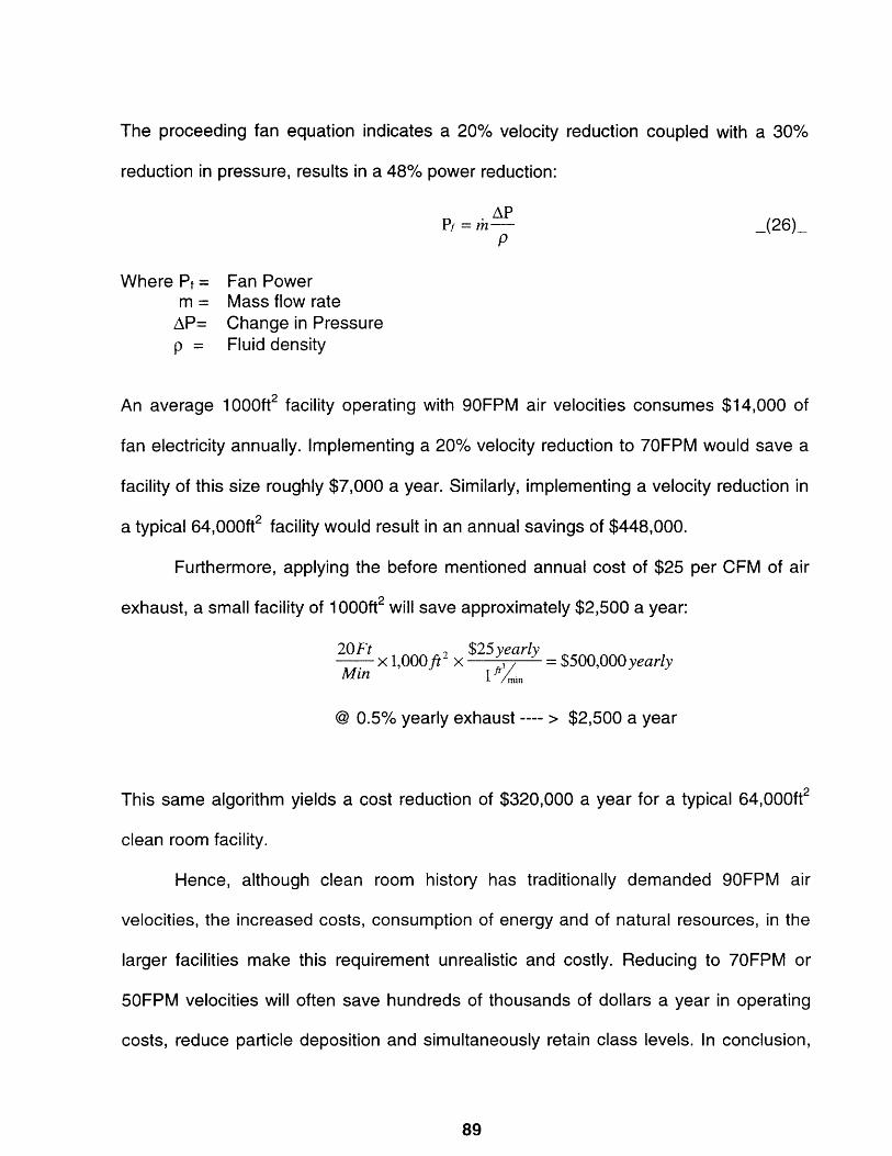
The proceeding fan equation indicates a 20% velocity reduction coupled with a 30%

reduction in pressure, results in a 48% power reduction:

APPi = rin- _(26)

P

Where Pf = Fan Powerm = Mass flow rate

AP= Change in Pressurep = Fluid density

An average 1000ft2 facility operating with 90FPM air velocities consumes $14,000 of

fan electricity annually. Implementing a 20% velocity reduction to 70FPM would save a

facility of this size roughly $7,000 a year. Similarly, implementing a velocity reduction in

a typical 64,000ft2 facility would result in an annual savings of $448,000.

Furthermore, applying the before mentioned annual cost of $25 per CFM of air

exhaust, a small facility of 1000ft2 will save approximately $2,500 a year:

20Ft $25 yearly- x 1,000ft2 x = $500,000yearlyMin 1 /n.

@ 0.5% yearly exhaust ---- > $2,500 a year

This same algorithm yields a cost reduction of $320,000 a year for a typical 64,000ft2

clean room facility.

Hence, although clean room history has traditionally demanded 90FPM air

velocities, the increased costs, consumption of energy and of natural resources, in the

larger facilities make this requirement unrealistic and costly. Reducing to 70FPM or

50FPM velocities will often save hundreds of thousands of dollars a year in operating

costs, reduce particle deposition and simultaneously retain class levels. In conclusion,

89

the results of this research warrant a paradigm shift to lower air velocities in operating

and future clean room facilities. Unique specifications for each clean room facility, will

prevent engineering design from antiquated models, significantly reduce operating

costs, and perhaps most importantly, limit the superfluous usage of energy and natural

resources from local communities.

5.6- Uncertainty Issues

5.6.1- Rake

Although the rake was positioned and constructed as stable as possible, due to

its height and slender body, it inevitably maintains a relative finite motion with respect to

ground. The swaying motion may cause additional crossflow measurements or even

falsely increase downflow measurements. However, these swaying motions occur at

extremely low frequencies. Because of the chosen sampling rate, this research

generates graphs from 0 to 100 kHz frequencies which facilitates the extraction of this

lower frequency data.

5.6.2 Probes

One key element of this research was the manufacture of hot wire anemometer

probes. Although the casings used were TSI models, due to the fragile nature of the

wires, the hot wires repeatedly disattached. To avoid high replacement fees from the

manufacturer, this research opted for spot welding methods to repair broken

anemometers. The disadvantage of this method is that each probe wire varies a finite

amount in length based on human error or craftsmanship. Spatial resolution is limited

90

by the length of the wire and different length hot wire anemometers will lead to a

variation of heat transfer and temperature across the wire.

Another accuracy issue may be raised with the electrical circuit. As mentioned

earlier, each design incorporates two potentiometers. These variable resistors provide

large benefits of enabling adjustable bias voltages, however, their strong disadvantage

is how easy it is to adjust this voltage unintentionally or after every use. Their

resistances are altered through screw switches which may easily turn on their own due

to movement or vibration. To compensate for this, potentiometer resistances were

calibrated with a voltmeter before every experiment to insure accurate values.

The Metrabyte Easyest LX software was chosen because of its ability to provide

a large frequency response to the data. Hot-Wire Anemometers have a high frequency

response and turbulence data would not have been possible with a sampling frequency

less than 10kHz. The frequency response data was gathered at a 100kHz sampling

frequency which permitted the acquisition of a large percentage of ranging fluctuations.

However, such a large sampling frequency became a limitation as the computer was

unable to store such large amounts of data for each test point. As a result, in order to

retain data values for each probe, the experiments were limited to using only a fraction

of a second after steady state had been reached. Although the time scale was short,

each probe data file contains a minimum of 64000 points. From calibration tests, the

computer software and hot wire data, the experimental apparatus has an uncertainty of

7%.

5.6.3- Facilities

One crucial aspect of these tests is the ability to accurately reduce air velocities

in the operating clean room; this was accomplished through a reduction in fan velocity.

However, the particular TRL facility has several fans feeding a combination of areas.

Hence, a fan reduction does not correspond to a one to one uniform velocity reduction

in the experimental space. To compensate for this issue, a hand held anemometer was

used to determine the velocity just downstream of each HEPA filter in the test grid. With

this test, experiments did not proceed until the velocity across each HEPA was uniform

and equal in magnitude. Although usage of hand held self calibrating instruments

during experiments is often frowned upon by researchers, in this instance it was most

certainly necessary and was virtually insignificant in the data acquisition itself.

5.7- Further Study

Although these tests have illustrated the strong dependency on particle

deposition to air velocities, they could not model the effects of personnel movement in

the clean room. Various studies have proven there are significant wakes behind moving

persons in clean rooms which would certainly effect the velocity profile and its purging

capacity. To make these test more comprehensive, further study incorporating clean

room operator movement in each velocity profile and measurement of the recovery time

for unidirectional airflow would be optimal.

Additionally, this research would have benefited greatly from the use of

computational fluid dynamics to model the experimental area. Since CFD may provide

over 100 times the resolution of these experiments, this data would have greatly

enhanced the reliability of the CFD predictions had they been done concurrently.

92

Bibliography

1. Austin, P.R. Design and Operation of Clean Rooms. Troy, Michigan: Business NewsPublishing Company, 1970. pp 1-9

2. Batchelor, H.K. The Theory of Homogeneous Turbulence. London: CambridgePress 1952 pp 5-14

3. Bowling, A., Davis, C. "Managing Contamination during advanced WaferProcessing," Solid State Technology February 1994 pp 45-47

4. Bradshaw, P. Turbulence and its Measurement New York: Spring Verlag 1978 pp128-131

5. Bradshaw, P. Turbulence New York: Springer Verlag 1978

6. Busnaina, A. "Modeling of Airflow and Particle Transport in Cleanrooms,"Proceedings, 10th ICCS 1990 International Symposium on Contamination Control pp276-280

7. Coleman, L.A. "Contamination Control Market to double by the Year 2000,"CleanRooms Magazine April 1996

8. Cooper, M.G. "Air Treatment Design for Clean Rooms," Building Design Partnership1993

9. Dunn, P.N. "The unexpected benefits of ISO 9000," Solid State Technology March1994 pp 55-57

10.English, S. "Handling/Delivery systems Keep Vigorous Pace with SemiconductorGrowth," CleanRooms magazine, March 1996 pp 20-28

11. George, W.K., Buether, P.D., Shabbier, A. "Polynomial Calibration for Hot-Wires inThermally varying Flows," 1987 Fluids Symposium on Thermal Anemometry pp 36-47

12. Hattori, T. "Contamination Control: Problems and Prospects," Solid StateTechnology July 1990 pp 45-51

13. Heyns, M. "Ultra-Clean or 'just clean enough' Technology?," Solid State TechnologyDecember 1994 p 23

14. Hinze, O.J. Turublence. New York: McGraw-Hill 1975

15. Hunt, Phillips, Williams Turbulent and Stochastic Processes: Kolmogorov's Ideas 50Years on. London: Royal Society 1991

16.Jorgenson, F. "Measurement of Low Turbulence Flows using Hot WireAnemometry," Dantec Technologies Technical Paper 34590-2 pp 3-17

17. Jorgenson, F. "Signal Processing and Hot Wire Anemometry," Dantec TechnologiesTechnical Paper 34560-1 pp 2-5

18.Kozicki, M., Hoening, S., Robinson, P. Cleanrooms. Van Nostrand Reinhold, NewYork. 1991 pp 118-124

19.Leinhard, Ill. Measurements in Mechanical Engineering. Cambridge, Mass.: MITPress 1989

20.Leslie, D.C. Developments in theTheory of Turbulence. Oxford: Claredon Press1983

21.Lieberman, A. "Airborne Particles in Cleanrooms," Particle Measuring SystemsTechnical Paper 3456-82 April 1989

22. Marvell,G. "Minienvironment Air Flow Design," Solid Sate Technology, August 1993pp 47-51

23. Mei, R. "Dispersion of Particles with Non Linear Drag and Restoring Force inTurbulent Flows," 1993 ASME Gas Particle Flows pp 47-65

24. Murakami, S., Shinsuke, K. "3-D Numerical Simulation of Air Flow in Clean rooms byneams of a 2 Equation Model," ASHRAE 1987 Annual Meeting, Nashville, TN.

25. "Semiconductors: When the Chips are Down," The Economist, March 23, 1996 pp19-21

26. Soules, W. "Airflow Management," CleanRooms Conference East 1996 Proceedinqs

27.Stainback S., Nagabushara, N. "Review of Hot-Wire Anemometry Techniques andRange of their Applications," 1993 ASME Symposium on Thermal Anemometry pp3-34

28.Stock, D.E. "Particle dispersion in Flowing Gases," Journal of Fluids Engineering,March 1996 pp 21-32

29.Tan-Athichat, J., Nagib, H.M., Loehrke, R.I. "Interaction of Free Stream Turbulencewith Screens and Grids: A Balance Between Turbulent Scales," Journal of FluidMechanics, 114:501-528

30.Townsend, A.A. The Structure of Turbulent Flow. Cambride England: CambridgeUniversity Press 1976

31.WIS Automatic Wafer Inspection System Operating Instructions. AeroncaElectronics Inc. 1984 pp 2-7

94

I "Semiconductors: When the Chips are Down," The Economist, March 23, 1996 pp 19-212 Austin, P.R. Design and Operation of Clean Rooms. Troy, Michigan: Business News PublishingCompany, 1970. pp 1-93 Kozicki, M., Hoening, S., Robinson, P. Cleanrooms. New York: Van Nostrand Reinhold, 1991 pp 118-1244 Austin, P.R. Design and Operation of Clean Rooms. Troy, Michigan: Business News PublishingCompany, 1970. pp 1-95 Coleman, L.A. "Contamination Control Market to double by the Year 2000," CleanRooms Magazine, April19966 Kozicki, M., Hoening, S., Robinson, P. Cleanrooms. New York: Van Nostrand Reinhold 1991 pp 118-1247 Batchelor, H.K. TheTheory of Homogeneous Turbulence. London: Cambridge Press 1952 pp 5-148 Bradshaw, P. Turbulence and its Measurement New York: Spring Verlag 1978 pp 128-1319 Batchelor, H.K. TheTheory of Homoqeneous Turbulence. London: Cambridge Press 1952 pp 45-6110 J. Tan-Athicaht, H.M., Nagib, R.I. "Interaction of Free Stream Turbulence with Screens and Grids: Abalance between Turbulent Scales," Journal of Fluid Mechanics, 114 pp 501-52811 Soules, W. "Airflow Management," CleanRooms Conference East 1996 Proceedings12 English, S. "Handling/Delivery systems Keep Vigorous Pace with Semiconductor Growth," CleanRoomsmagazine, March 1996 pp 20-28

13 Lieberman, A. "Airborne Particles in Cleanrooms," Particle Measuring Systems Technical Paper 3456-82 April 198914 Mei, R. "Dispersion of Particles with Non Linear Drag and Restoring Force in Turbulent Flows," 1993ASME Gas Particle Flows pp 47-651T Busnaina, A. "Modeling of Airflow and Particle Transport in Cleanrooms," Proceedings, 10 th ICCS 1990International Symposium on Contamination Control pp 276-28016 English, S. "Handling/Delivery systems Keep Vigorous Pace with Semiconductor Growth," CleanRoomsmaqazine, March 1996 pp 20-28" Jorgenson, F. "Measurement of Low Turbulence Flows using Hot Wire Anemometry" DantecTechnologies Technical Paper 34590-2 pp 3-17

Leinhard, Ill. Measurements in Mechanical Engineering. Cambridge, Mass: MIT Press 198919 Stainback S., Nagabushara, N. "Review of Hot-Wire Anemometry Techniques and Range of theirApplications," 1993 ASME Symposium on Thermal Anemometry pp 3-34

Jorgenson, F. "Signal Processing and Hot Wire Anemometry" Dantec Technologies Technical Paper3456-7 pp 2-521 WIS Automatic Wafer Inspection System Operating Instructions. Aeronca Electronics Inc. 1984 pp 2-7

Batchelor, H.K. TheTheory of Homogeneous Turbulence. London: Cambridge Press 1952 pp 4-21

95