Jurnal Kejuruteraan 17 (2005) 27-32

Comparing Linear and Bilinear Models on Water Level for the Kelantan River in Malaysia

Azami Zaharim, Mohd Sahar Yahya, Ibrahim Mohamed, Abdul Halim Ismail, Zuhairuse Md Darus and Zulkitli Mohd Nopiah

ABSTRACT

Surveyed from 160 time series data used in scientific articles concluded that 10-13% of them were generated by the nonlinear process. Several nonlinear models are available but only the bilinear model will be considered here. The bilinear model is basically an extension of the linear model ARlMA. 1t was first introduced by control theorists in 1972 before it was documented by Granger and Anderson in 1978. The bilinear model is believed to be able to fit hydrological and meteorological data well. 1n this paper, the coefficients of a special case of bilinear model, BL( 1,1,1,1), are estimated using nonlinear least squares method. Results of modeling the linear and bilinear models on water level data from the Kelantan river in Malaysia when compared and evaluated gave better fitting to the bilinear model.

Keywords: Bilinear, ARIMA models, nonlinear, water level

ABSTRAK

Tinjauan ke atas 160 data siri masa di dalam artikel saintifik menyimpulkan bahawa 10-13% daripadanya dijanakan melalui proses tak linear. Terdapat beberapa model tak linear tetapi model bilinear sahaja yang akan di pertimbangkan dalam artikel ini. Model bilinear secara asasnya adalah lanjutan daripada model linear ARIMA. Model ini telah diperkenalkan oleh teoris kawalan pada tahun 1972 sebelum didokumenkan oleh Granger dan Anderson dalam tahun 1978. Model bilinear dipercayai mampu untuk memodelkan data hidrologi dan data meteorologi dengan baik. Dalam artikel ini, pekali bagi kes khusus model bilinear BL(1,1,1,1) telah dianggar menggunakan kaedah tak linear kuasa dua terkecil. Keputusan melalui pemodelan model linear dan bilinear ke atas data aras air dari sungai Kelantan di Malaysia setelah dibanding dan dinilai memberi ketepatan lebih baik terhadap model bilinear.

Kata kunci: Bilinear, model ARIMA, tak linear, aras air

INTRODUCTION

Water level has been used as an indicator to the occurrence of flooding. The univariate Box-Jenkins approach based on ARIMA modeling has been used in many applications. A good account of the approaches is available in, inter alia, (Box & Jenkins 1976; Chatfield 1996; Fuller 1976). However, there are time series data which are not suitable to be fitted by linear models such as the Castle river flow data in Alberta, Canada (Oyet 2001) and the average

28

monthly flows of the Fraser river in British Columbia (Lewis & Ray 2002). These data might be fitted better by a nonlinear model such as the bilinear model. In this article, a comparative study between ARIMA models and the bilinear model is discussed.

DATA COLLECTION

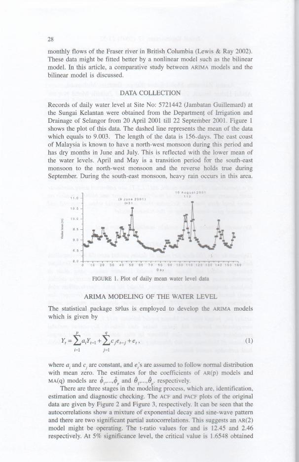
Records of daily water level at Site No: 5721442 (Jambatan Guillemard) at the Sungai Kelantan were obtained from the Departmen~ of Irrigation and Drainage of Selangor from 20 April 2001 till 22 September 2001. Figure 1 shows the plot of this data. The dashed line represents the mean of the data which equals to 9.003. The length of the data is 156.days. The east coast of Malaysia is known to have a north-west monsoon durin~ thi period and has dry months in June and July. This is reflected with the lower mean of the water levels. April and May is a transition period for the south-east monsoon to the north-west monsoon and the reverse hold true during September. During the south-east monsoon, heavy rain occur in this area.

11.0

10 5

I 100

I • 5 l! ~

• 0

8 5

8.0

(9 June 2001) t- 51

10 August 200' 113

10 20 3 0 "0 50 60 70 80 00 100 ItO 120 ,'0 '&0 150 1&0

o oy

FIGURE 1. Plot of daily mean water level data

ARIMA MODELING OF THE WATER LEVEL

The statistical package splus is employed to develop the ARThtA models which is given by

p q

Yt = La;Yt - 1 + Lcje t - j +e t , (1)

;=1 j=1

where a. and c. are constant, and e's are assumed to follow normal distribution I ) r

with mean zero. The estimates for the coefficient of AR(p) models and MA(q) models are $1'''''~P and 8" ... ,8p' respectively.

There are three stages in the modeling process, which are. identification, estimation and diagnostic checking. The ACF and PACF pIa of the original data are given by Figure 2 and Figure 3, respectivel). It can be een that the autocorrelations show a mixture of exponential decay and ine-wave pattern and there are two significant partial autocorrelations. Thi ugge ts an AR(2) model might be operating. The t-ratio values for and i 12.45 and 2.46 respectively. At 5% significance level, the critical value i 1.6548 obtained

29

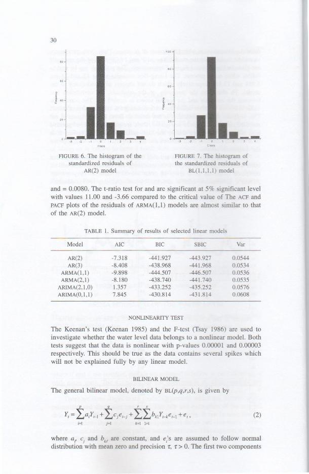
from the t-distribution with 154 degree of freedom. Thus, both parameters should be included in the model. The ACF and PACF plots of the residuals are given in Figure 4 and Figure 5 respectively. The residuals can be said to follow white noise process. The Ljung-Box statistics at lag 12 and 24 are 5.884 and 12.111 respectively which do not suggest any inadequacy to the model. To check on the normality of the residuals, the correlation test between the residuals and the normal scores is carried out. The correlation value is 0.9056 which is below the corresponding 5% critical value of 0.987. This suggests that the normality is not satisfied. From the histogram of the standardized residuals given in Figure 7, there are quite a number of positive high residuals which are due to the high spikes in the data earlier. It is believed that detecting these outliers and adjusting their effects will improve the diagnostic results.

Several other linear models are also fitted in order to find out whether other ARIMA models can improve the modeling. The various models will be compared based on three types of order selection criteria. They are the Akaike's information criteria denoted by AIC (Akaike 1969), Akaike's Bayesian information criteria denoted by BIC (Akaike 1974) and Schwarz's criteria denoted by SBIC (Schwarz 1978). Based on these criteria, it is found out that ARMA(1,1) improves the modeling with = 0.722, = -0.327, = 0.0043

1.0

0.8

06

.0.'

.os

.o8

·1.0

.()4

FIGURE 2. The ACF plot of the water level data

FIGURE 4. The ACF plot of residuals of AR(2) model

.Q4

.QS

.()8

-to

FIGURE 3. The PACF plot of the water level data

Q4

02

~OO+~,L~~LL~~~~-'rrT;~

"-.Q2

. 1<tJ

FIGURE 5. The PACF plot of residuals of AR(2) model

30

a.

a.

j ..

,.

FIGURE 6. The histogram of the standardized residuals of

AR(2) model

, .. "

a.

, . . ,

c ..

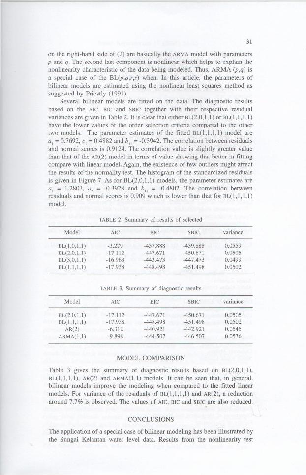
FIGURE 7. The histogram of the standardized re iduals of

BL(l,l.l.l ) model

and = 0.0080. The t-ratio test for and are significant at 5 'k: ignificant level with values 11.00 and -3.66 compared to the critical value of The ACF and PACF plots of the residuals of ARMA(1,1) models are almo t imilar to that of the AR(2) model.

TABLE 1. Summary of results of selected linear model

Model AIC BIC SBIC Var

AR(2) -7.318 -441.927 -443.927 0.0544 AR(3) -8.408 -438.968 -441.968 0.0534

ARMA(l ,I ) -9.898 -444.507 -446.507 0.0536 ARMA(2,1) -8.180 -438.740 -441.740 0.0535

ARIMA(2, 1 ,0) 1.357 -433.252 -435.252 0.0576 ARIMA(O,I,I) 7.845 -430.814 -431.814 0.0608

NONLINEARITY TEST

The Keenan's test (Keenan 1985) and the F-test (Tsay 1986) are used to investigate whether the water level data belongs to a nonlinear model. Both tests suggest that the data is nonlinear with p-values 0.0000 1 and 0.00003 respectively. This should be true as the data contains several spikes which will not be explained fully by any linear model.

BILINEAR MODEL

The general bilinear model, denoted by BL(p,q,r ,s), is given by

p q r s

Y, = L a;Yt-l + Lcje,_j + LLbklY,-ke'-l +e" (2) i=l j=1 k=1 1=1

where a., c. and bkl

are constant, and e's are assumed to follow normal I } ,

distribution with mean zero and precision 'l', 'l' > O. The fIrst two components

31

on the right-hand side of (2) are basically the ARMA model with parameters p and q. The second last component is nonlinear which helps to explain the nonlinearity characteristic of the data being modeled. Thus, ARMA (p ,q) is a special case of the BL(p,q,r,s) when. In this article, the parameters of bilinear models are estimated using the nonlinear least squares method as suggested by Priestly (1991).

Several bilinear models are fitted on the data. The diagnostic results based on the Ale, Ble and SBle together with their respective residual variances are given in Table 2. It is clear that either BL(2,0,1 ,1) or BL(1,I,I , I) have the lower values of the order selection criteria compared to the other two models. The parameter estimates of the fitted BL(1 ,I,I,l) model are a

l = 0.7692, c

1 = 0.4882 and b

ll = -0.3942. The correlation between residuals

and normal scores is 0.9124. The correlation value is slightly greater value than that of the AR(2) model in terms of value showing that better in fitting compare with linear model. Again, the existence of few outliers might affect the results of the normality test. The histogram of the standardized residuals is given in Figure 7. As for BL(2,0,1,1) models, the parameter estimates are a

l = 1.2803, a

2 = -0.3928 and b

ll = -0.4802. The correlation between

residuals and normal scores is 0.909 which is lower than that for BL(1,I,I ,I) model.

TABLE 2. Summary of results of selected

Model Ale Ble SBle variance

BL(1,0,1,l) -3.279 -437.888 -439.888 0.0559 BL(2,0,1,1) -17.112 -447.671 -450.671 0.0505 BL(3,0,1,1) -16.963 -443.473 -447.473 0.0499 BL(1 ,I,l,l) -17.938 -448.498 -451.498 0.0502

TABLE 3. Summary of diagnostic results

Model Ale Ble SBle variance

BL(2,0,1,1) -17.112 -447.671 -450.671 0.0505 BL(1 ,1,1,1) -17.938 -448.498 -451.498 0.0502

AR(2) -6.312 -440.921 -442.921 0.0545 ARMA(1 ,1) -9.898 -444.507 -446.507 0.0536

MODEL COMPARISON

Table 3 gives the summary of diagnostic results based on BL(2,0,1,1), BL(1,I,I , I), AR(2) and ARMA(I,I) models. It can be seen that, in general, bilinear models improve the modeling when compared to the fitted linear models. For variance of the residuals of BL(1,I,I,l) and AR(2), a reduction around 7.7% is observed. The values of Ale, Ble and SBre are also reduced.

CONCLUSIONS

The application of a special case of bilinear modeling has been illustrated by the Sungai Kelantan water level data. Results from the nonlinearity test

32

confirm that the data are nonlinear. The modeling result further show that bilinear model fits better compared to linear models.

ACKNOWLEDGEMENT

The original data is obtained from the Department of Irrigation and Drainage, Selangor, D.E.

REFERENCE

Akaike, H. 1969. Fitting autoregressive model for prediction. Annals Institute of Statistical Mathematics 21: 203-217.

Akaike, H. 1979. A Bayesian extension of the minimum AlC procedure of autoregressive modeling. Biometrika 66: 237-242.

Box, G.E.P. & Jenkins, G.M. 1976. Time Series Analysis Forecasting and Control. San Francisco: Holden-Day.

Chatfield, C. 1996. The Analysis of Time Series: An Introduction. London: Chapman and Hall.

Fuller, W.A. 1976. Introduction to Statistical Time Series . ew York: Wiley. Keenan, D. M. 1985. A Tukey non-additivity type test for time erie nonlinearity.

Biometrika 72(1): 39-44. Lewis, P.A.W. & Ray, B.K. 2002. Nonlinear modeling of periodic threshold auto­

regressions using TSMARS. Journal of Time Series Analysis 23(4): 272-285. Oyet, A.J. 200l. Nonlinear time series modeling: Order identification and wavelet

filtering. Interstat, April 200l. Priestly, M.B. 1991. Non-linear and Non-stationary Time Series Analysis. San

Diego: Academic Press. Schwarz, G. 1978. Estimating the dimension of a model. Annals of Statistics 6: 461-

464. Tsay, R.S. 1986. Nonlinearity test for time series. Biometrika 73(2): 461-466.

Azami Zaharim Abdul Halim Ismail Zuhairuse Md Darus Department of Archtitecture Faculty of Engineering Universiti Kebangsaan Malaysia 43600 UKM Bangi, Selangor D.E.

Mohd. Sahar Yahya Matriculation Centre Universiti Malaya 50603 Kuala Lumpur

Ibrahim Mohamed Institute of Mathematical Sciences Universiti Malaya 50603 Kuala Lumpur

Zulkifli Mohd Nopiah Department of Mechanical and Material Faculty of Engineering Universiti Kebangsaan Malaysia 43600 UKM Bangi, Selangor D.E.