DESIGN AND TESTING OF AN EVAPORATIVE COOLING SYSTEM

USING AN ULTRASONIC HUMIDIFIER

KAEL EGGIE

ADVISOR: DR. G.S.V. RAGHAVAN

Kael Eggie

Student Branch Faculty

Advisor:

Dr. G.S.V. Raghavan

Department of Bioresource Engineering

Room MS1-027, Macdonald-Stewart Building, 21111 Lakeshore Road

Ste. Anne de Bellevue, Quebec H9X 3V9

Tel.: 514-398-7773 | Fax: 514-398-8387

Date of signing: May 12, 2008

2

STATEMENT OF PURPOSE

This paper topic was chosen at the behest of the course coordinator, Dr. Raghavan, who wanted

work to be performed with a client’s (Plastique Frapa Inc.) humidifying technology in relation to

part of his research interest area: postharvest storage.

This paper was part of a senior year design project and reports the results of the experiment work

that was performed in analyzing the effectiveness of the designed setup. Aside from the topic

definition, the project was self-directed in terms of methodology and analysis. Although it

should be noted that research associates of the department were instrumental in solving problems

that occurred throughout the experimentation.

A co-author for this paper must be recognized for his contributions to the formulation of this

paper. Michael Schwalb, worked very closely to assist in setup, conceptualization and other

technical aspects.

3

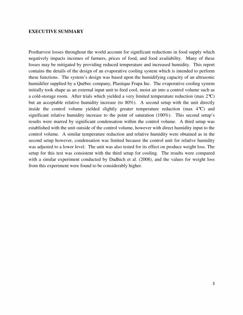
EXECUTIVE SUMMARY

Postharvest losses throughout the world account for significant reductions in food supply which

negatively impacts incomes of farmers, prices of food, and food availability. Many of these

losses may be mitigated by providing reduced temperature and increased humidity. This report

contains the details of the design of an evaporative cooling system which is intended to perform

these functions. The system’s design was based upon the humidifying capacity of an ultrasonic

humidifier supplied by a Québec company, Plastique Frapa Inc. The evaporative cooling system

initially took shape as an external input unit to feed cool, moist air into a control volume such as

a cold-storage room. After trials which yielded a very limited temperature reduction (max 2°C)

but an acceptable relative humidity increase (to 80%). A second setup with the unit directly

inside the control volume yielded slightly greater temperature reduction (max 4°C) and

significant relative humidity increase to the point of saturation (100%). This second setup’s

results were marred by significant condensation within the control volume. A third setup was

established with the unit outside of the control volume, however with direct humidity input to the

control volume. A similar temperature reduction and relative humidity were obtained as in the

second setup however, condensation was limited because the control unit for relative humidity

was adjusted to a lower level. The unit was also tested for its effect on produce weight loss. The

setup for this test was consistent with the third setup for cooling. The results were compared

with a similar experiment conducted by Dadhich et al. (2008), and the values for weight loss

from this experiment were found to be considerably higher.

4

ACKNOWLEDGEMENTS

Throughout the duration of our project, we had quite a bit of help along the way. We relied on

the experience and knowledge of a number of people who were able to point us in the right

direction regarding a starting point or how to navigate around the many road blocks we

encountered.

Our first thanks go to M. Yvan Gariepy who gave much of his time. His expertise in problem

solving, instrumentation instruction and general testing design was instrumental in the

completion of this project.

We would also like to thank Dr. Sam Sotocinal who lended his opinion to the setup design,

guiding around the machine shop and helping troubleshoot when problems arose.

Dr. Raghavan warrants our thanks for providing the project as well as being a guide for project

definition.

5

TABLE OF CONTENTS

STATEMENT OF PURPOSE ...................................................................................................................... 2

ACKNOWLEDGEMENTS .......................................................................................................................... 4

TABLE OF CONTENTS .............................................................................................................................. 5

LIST OF FIGURES ...................................................................................................................................... 6

INTRODUCTION ........................................................................................................................................ 7

METHOD AND MATERIALS .................................................................................................................. 10

THE ULTRASONIC HUMIDIFYING UNIT ............................................................................................ 10

DESIGN OF A MIXING CHAMBER ....................................................................................................... 10

Design Concerns and Considerations for a Mixing Chamber ................................................................. 11

Testing Setup .......................................................................................................................................... 12

EVAPORATIVE COOLING SYSTEM DESIGN ..................................................................................... 16

Design Parameters .................................................................................................................................. 16

Evaporative Cooling Design Set-Up: ...................................................................................................... 16

Testing Procedure of Evaporative Cooling Unit ..................................................................................... 17

EVAPORATIVE COOLING EFFECTS ON PRODUCE .......................................................................... 25

LIMITATIONS AND SETBACKS ............................................................................................................ 30

CONCLUSIONS......................................................................................................................................... 30

REFERENCES ........................................................................................................................................... 31

APPENDIX A – Performance Analysis of Mixing Chamber at Varying Maximum Air Velocities .......... 32

APPENDIX B – Solid Works Representational Model .............................................................................. 35

APPENDIX C – Diagram of MDFD-1 Ultrasonic Humidifier by Plastique Frapa Inc. ............................. 36

APPENDIX D – Thermal Load Analysis ................................................................................................... 37

6

APPENDIX E – Calculation of Relative Humidity from Tdry and Twet ....................................................... 39

APPENDIX F – Daily Weight Loss of Produce ......................................................................................... 42

APPENDIX G – Psychrometric Chart ........................................................................................................ 44

APPENDIX H - Ideal Mixing Chamber Velocity....................................................................................... 45

LIST OF FIGURES

Figure 1 - Images of parallel and series configurations ................................................................ 12

Figure 2 - Initial Test Results: RH and Tdry vs. time .................................................................... 13

Figure 3 - Initial Test Results: Tdry and Twet vs. time .................................................................... 14

Figure 4 - Performance curve relating Tdry and RH to air velocity ............................................. 15

Figure 5 - First Setup: Humidifying unit outside control volume ................................................ 17

Figure 6 - Relative Humidity, Tdry,CV vs. time with unit outside control volume ..................... 19

Figure 7 - Tdry,ambient vs. time for unit outside control volume ................................................ 19

Figure 8 – Tdry,ambient – Tdry,CV vs. time for unit outside control volume ............................. 20

Figure 9 - Second Setup: Humidifying unit inside control volume .............................................. 22

Figure 10 – Tdry,CV vs. time with unit inside control volume .................................................... 23

Figure 11 – Tdry,ambient vs. time for unit inside control volume* ............................................. 24

Figure 12 - Tdry,ambient – Tdry,CV vs. time with unit inside control volume* ......................... 24

Figure 13 - RH and Tdry inside control volume vs. time ............................................................... 26

Figure 14 - RH and Tdry vs. time outside control volume ............................................................. 26

Figure 15 - Carrot weight loss vs. time ......................................................................................... 27

Figure 16 - Radish weight loss vs. time ........................................................................................ 28

Figure 17 - Spinach weight loss vs. time ...................................................................................... 28

7

INTRODUCTION

The global population in the year 2008 has hit an unprecedented level of 6.5 billion. It continues

to rise drastically, and is predicted to hit 8 billion by the year 2025 (United Nations, 2008). In

addition, with the economic rise of highly populous countries such as China and India, there is

also an unprecedented rise in the overall global standard of living. From an agriculture

perspective, these facts translate into an immense increase in the demand for food. Naturally, this

entails a subsequent increase in the price of food and agricultural products worldwide. It should

also be noted that industries such as the biofuel industry constitute market forces that contribute

to the rise in the demand and price of agricultural products. Agricultural engineers are faced with

the task of not only meeting the food requirements of the ever increasing global population, but

to also maintain relatively low costs for food products. From basic economics principles,

stabilizing the cost of a product undergoing an increase in its demand requires either an increase

in its supply or a decrease in its cost of production. However, with agricultural products, such a

task is not so simple: the amount of land that can be cultivated has reached its practical limit.

Furthermore, soaring energy prices continue to push the costs of production from the growing

stage to the transportation stage of production higher and higher. The only possible way left to

stabilize the cost of food is to establish and implement new and efficient methods for crop

production, post-harvest drying and storage, as well as distribution and transportation. It should

be noted, that such Although all of these aspects are important when trying to tackle the

challenge of meeting stabilizing the cost of food, this design project only explores the post

harvest storage aspect of food production. In southeast Asia, postharvest losses range from 10%-

37% for rice (International Rice Commission, 2002). Furthermore, in India, post harvest losses

are in the range of 25-50%. These losses translate into a significant loss in the overall supply of

agricultural products.

To realize the relevance of this project it is important to recognize the reasons for postharvest

losses in relation to temperature and humidity. Losses related to temperature and humidity can

include spoilage due to disease, over-ripening, negative physiological and compositional effects,

loss of mass (produce water mass), and aesthetic appeal. The goals of postharvest cooling are to

counteract these effects by the following mechanisms:

-slow and inhibit water loss

-suppress enzymatic degradation and respiration

-slow and inhibit the growth rate and activity of pathogens

-reduce the production of ethylene or minimize a commodity’s reaction to ethylene

(Narayanasamy, 2006)

8

Some background on each aspect is necessary in understanding why it is important to analyze

and correct this problem. The first problem of water loss is related to food structure, texture and

appearance changes. Water loss after harvest is mainly dependent on two things: 1. the water

vapour pressure deficit that exists between produce and its immediate environment, and 2. the

surface transfer resistance to water vapour movement (determined by shape and internal

resistances as well as surface resistances) which occurs now that the plant is no longer

transpiring through its stomata. Transpiration resistance can be increased as a boundary layer of

water vapour-saturated air is fashioned because of zero air movement, but the interrelation of

factors can be seen in this case because to remove respiratory heat there must be air convection,

so a balance must be found. Water loss affects commodities’ quality and taste in that water

increases the turgor pressure of fruits and vegetables which lends itself to a perceived

“freshness” and “crispness” upon consumption. (Wills et al., 2007)

Very important to the economic side of production is that that fruits and vegetables are largely

sold on the basis of weight, loss of water is indicative of a loss in revenue which farmers can ill

afford.

Suppressing respiration is integral in food preservation; respiration refers to the breakdown of

sugars and other compounds within the cell which releases carbon dioxide, water and heat to the

surroundings (linking respiration to water loss). It is important to note that the rate of metabolic

activity in cells increases with temperature; thus the importance of minimizing produce

temperature (and environment temperature) is clear. Produce is typically harvested at ideal times

(i.e. ripeness) depending on whether or not it is considered climacteric or non-climacteric, but

remains a living entity; thus, cells perform the normal functions of aging (DeEll et al., 2003).

Eventually a stage of senescence is reached whereby the cell continues respiring, but loses the

ability to divide and becomes a dying entity. During the stage of senescence, cell-wall structure

and composition changes and subsequently produce may become more palatable to a point, but

these changes make the produce more susceptible to damage from external forces.

Also involved in ripening and eventual produce edibility and/or degradation is the chemical

ethylene which is a hormone that may be either produced naturally by the commodity, or applied

as a catalyst to hasten the ripening process. There is a large variability between commodities in

terms of the actual production rate of ethylene and the commodities’ response to ethylene. The

final effect of pre-cooling treatments that are implemented is to improve the limitation of

pathogens and disease found in vegetables. Postharvest diseases causing spoilage in perishable

commodities can be significant as shown by Table 1.1 in Narayanasamy (2006). Pathogens and

disease tend to flourish in high temperature and high humidity environments and produce may

become affected at any point in the postharvest pathway to the consumer; in terms of pre-

cooling, removing initial field heat is an important first step to limiting the influence of diseases.

9

Moreover, there is a tradeoff to be made with respect to humidity control and it is certainly

beneficial to have a high humidity environment for fruits and vegetables with regard to water

loss, but leaves the produce more susceptible to disease; another important management decision

for producers.

Evaporative cooling is of specific interest to engineers concerned with the efficiency and energy

demands of post-harvest storage. While providing a humid environment required for storage,

humidifiers also offer the potential to provide some cooling. However, this is only the case with

mechanical humidifiers and not with traditional humidifiers that use a heating element to

evaporate water. The theory behind cooling effect from evaporation is simple: as water

evaporates it absorbs latent heat from the surroundings (notably air) and as a result the ambient

temperature is reduced. This phenomenon is precisely why a human being feels cooler when

sweating.

In the context of food storage, much research has been done to explore the effects that

evaporative cooling may have for extended preservation by counteracting the previously

discussed activities of stored produce. In a study which examined the benefits of evaporative

cooling for tomato storage by Mordi and Olurunda (2003), an average drop of 8.2°C in

comparison to ambient temperature was observed. Also, an increase in relative humidity of 36%

was experienced. These changes in air quality had a significant impact on the storage life of the

tomatoes as within the evaporative cooling unit, the tomatoes were stored for 11 days in

comparison to 4 days of ambient conditions storage. Another study by Dadhich et al. (2008) also

demonstrated significantly improved storage life for a number of different commodities due to a

simple evaporative cooling technology. In their comparative study between an evaporative

cooling environment (0.7 m3 brick structure) and ambient conditions, % weight loss and visual

quality were the factors of concern. After 7 days, produce within the evaporative cooler retained

much more of its moisture as compared to the ambient conditions. For example, carrots lost 5%

and 50% of their mass between the respective conditions and coriander leaves lost 15% and 76%

of their mass. In a study by Thiagu et al. (1990) it was demonstrated that moisture loss in

tomatoes is 6.5 times as great in ambient conditions (28°C – 33°C, 45%-65% RH) as in

evaporative cooling conditions (20°C – 25°C, 92%-95%). They also demonstrated that lycopene

development is significantly higher (double in this case) in evaporative cooling storage

conditions than ambient conditions.

Plastique Frapa Inc., a small humidifier manufacturer has been exploring the benefits of an

ultrasonic mechanical humidifier. The unit itself produces droplets in the range of 1-5 microns

compared to specialized fine nozzle diffusers that produce droplets in the range of 70-80

microns. The advantage of the smaller water droplets are less condensation and greater

evaporation rate. The goal of this design project is to explore and test an ultrasonic unit in order

to identify its potential for use in a storage environment. As such, an evaporative cooling system

will be design and built the in order to determine the cooling effect, if any, of the unit. Again,

10

this cooling effect has the potential to significantly reduce the energy requirements of a storage

system. After such tests, the unit will also be tested for its ability to disperse humidity and

droplets into a storage volume. A complete storage environment with a controlled atmosphere

will, however not be created and such design details are beyond the scope of this project. It

should be noted that the unit itself will only be tested for cooling effect, and the ability to provide

humidity without making condensation. The hypothesis is that the humidifier will provide

significant cooling and little condensation will occur when used.

METHOD AND MATERIALS

THE ULTRASONIC HUMIDIFYING UNIT

The ultrasonic humidifier, as already mentioned, is manufactured by a small humidifier company

called Plastique Frapa. The unit comprises of a water reservoir, a fan, and a small mechanical

vibrating transducer. The reservoir is attached to the transducer by a small hose and provides

water, through a slight pressure head difference, at such a rate that there is always a thin layer of

water sitting on top of the transducer. When the unit is operating, the transducer vibrates

ultrasonically with a frequency of roughly 1.65MHz. These mechanical oscillations break the

thin layer of water into extremely fine water droplets. The water in the reservoir completes a

circuit with the transducer and the fan and is controlled through a simple pinch float mechanism.

When the water level in the reservoir is too low, the circuit is broken and the unit is no longer in

operation. The unit also has very low power consumption of 48 watts and more specifically

operates at a voltage of only 48 volts and a current of only one amp.

DESIGN OF A MIXING CHAMBER

There are two reasons why a mixing chamber is a key component to a storage system design.

The first is to continuously provide moisture and air into the control volume and the second is to

properly disperse it. Properly dispersing the water droplets outside the control volume is

hypothesised to reduce the amount of condensation occurring within the control volume.

Dispersing the air and water droplets outside the control volume also has the advantage of

keeping the heat loss from the mixing fan outside the control volume. Nevertheless, the

hypotheses and assumptions about the benefits of using a mixing chamber were verified by

designing and building an evaporative cooling system without a mixing chamber. The amount of

cooling and condensation that occurred with and without a mixing chamber will be compared

and evaluated. The results of these tests will be presented and discussed in the following section

of the paper.

11

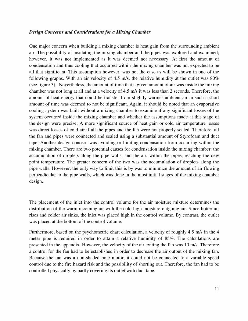
Design Concerns and Considerations for a Mixing Chamber

One major concern when building a mixing chamber is heat gain from the surrounding ambient

air. The possibility of insulating the mixing chamber and the pipes was explored and examined;

however, it was not implemented as it was deemed not necessary. At first the amount of

condensation and thus cooling that occurred within the mixing chamber was not expected to be

all that significant. This assumption however, was not the case as will be shown in one of the

following graphs. With an air velocity of 4.5 m/s, the relative humidity at the outlet was 80%

(see figure 3). Nevertheless, the amount of time that a given amount of air was inside the mixing

chamber was not long at all and at a velocity of 4.5 m/s it was less than 2 seconds. Therefore, the

amount of heat energy that could be transfer from slightly warmer ambient air in such a short

amount of time was deemed to not be significant. Again, it should be noted that an evaporative

cooling system was built without a mixing chamber to examine if any significant losses of the

system occurred inside the mixing chamber and whether the assumptions made at this stage of

the design were precise. A more significant source of heat gain or cold air temperature losses

was direct losses of cold air if all the pipes and the fan were not properly sealed. Therefore, all

the fan and pipes were connected and sealed using a substantial amount of Styrofoam and duct

tape. Another design concern was avoiding or limiting condensation from occurring within the

mixing chamber. There are two potential causes for condensation inside the mixing chamber: the

accumulation of droplets along the pipe walls, and the air, within the pipes, reaching the dew

point temperature. The greater concern of the two was the accumulation of droplets along the

pipe walls. However, the only way to limit this is by was to minimize the amount of air flowing

perpendicular to the pipe walls, which was done in the most initial stages of the mixing chamber

design.

The placement of the inlet into the control volume for the air moisture mixture determines the

distribution of the warm incoming air with the cold high moisture outgoing air. Since hotter air

rises and colder air sinks, the inlet was placed high in the control volume. By contrast, the outlet

was placed at the bottom of the control volume.

Furthermore, based on the psychometric chart calculation, a velocity of roughly 4.5 m/s in the 4

meter pipe is required in order to attain a relative humidity of 85%. The calculations are

presented in the appendix. However, the velocity of the air exiting the fan was 10 m/s. Therefore

a control for the fan had to be established in order to decrease the air output of the mixing fan.

Because the fan was a non-shaded pole motor, it could not be connected to a variable speed

control due to the fire hazard risk and the possibility of shorting out. Therefore, the fan had to be

controlled physically by partly covering its outlet with duct tape.

12

After the right duct tape configuration was found in order to restrict the fan’s air velocity to 4.5

m/s, a test was run in order to examine and compare the air quality at the inlet of the mixing

chamber and the outlet of the mixing chamber. This initial test was run with a parallel

configuration, in that the fan was connected to the mixing chamber in parallel with the

humidifier. The following photo depicts the parallel and series configuration used for the mixing

chamber.

Figure 1 - Images of parallel and series configurations

The following testing setup was used in order to examine the effect of the mixing chamber on the

quality of air. Again, the setup of the experiments, is shown in the photo above.

Testing Setup

Materials

-4 Thermocouples

-data logger

-computer

-wet bulb readers

-2 x 4” pipe

-humidifier

-continuously running time data logger

13

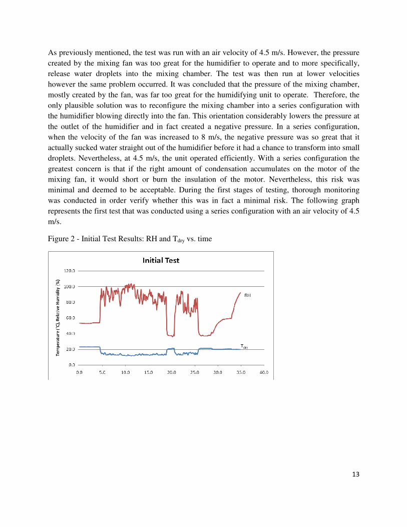
As previously mentioned, the test was run with an air velocity of 4.5 m/s. However, the pressure

created by the mixing fan was too great for the humidifier to operate and to more specifically,

release water droplets into the mixing chamber. The test was then run at lower velocities

however the same problem occurred. It was concluded that the pressure of the mixing chamber,

mostly created by the fan, was far too great for the humidifying unit to operate. Therefore, the

only plausible solution was to reconfigure the mixing chamber into a series configuration with

the humidifier blowing directly into the fan. This orientation considerably lowers the pressure at

the outlet of the humidifier and in fact created a negative pressure. In a series configuration,

when the velocity of the fan was increased to 8 m/s, the negative pressure was so great that it

actually sucked water straight out of the humidifier before it had a chance to transform into small

droplets. Nevertheless, at 4.5 m/s, the unit operated efficiently. With a series configuration the

greatest concern is that if the right amount of condensation accumulates on the motor of the

mixing fan, it would short or burn the insulation of the motor. Nevertheless, this risk was

minimal and deemed to be acceptable. During the first stages of testing, thorough monitoring

was conducted in order verify whether this was in fact a minimal risk. The following graph

represents the first test that was conducted using a series configuration with an air velocity of 4.5

m/s.

Figure 2 - Initial Test Results: RH and Tdry vs. time

14

Figure 3 - Initial Test Results: Tdry and Twet vs. time

The humidifier was only started after the 4 minute mark. This point is marked by the

instantaneous drop in Twet and Tdry in the above graph. The relative humidity was calculated by

measuring both the wet bulb and dry bulb temperatures and then by calculating the relative

humidity. However, measuring the wet bulb is not a simple task. In order to truly measure the

wet bulb temperature, a wick on a thermocouple must be constantly saturated but not saturated to

the point where droplets form on its surface. From the graph, before the humidifier was even

started, the relative humidity was calculated to be 60%, which was far from the 22% value

measure for ambient air. The dry bulb temperatures at the outlet of the mixing chamber were

consistent with ambient dry bulb temperatures. Therefore, it was concluded that there were errors

in precision of our wet bulb readings and another method for measuring relative humidity was

needed. Data loggers were then used and placed at the outlet and the inlet of the mixing chamber.

These data loggers measure relative humidity directly.

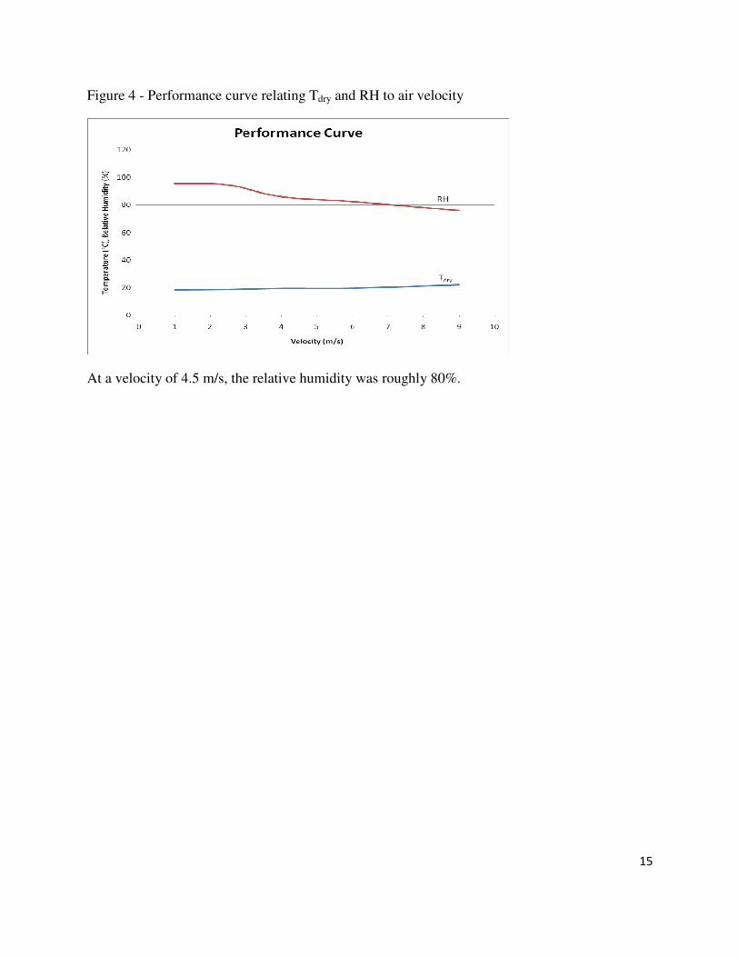
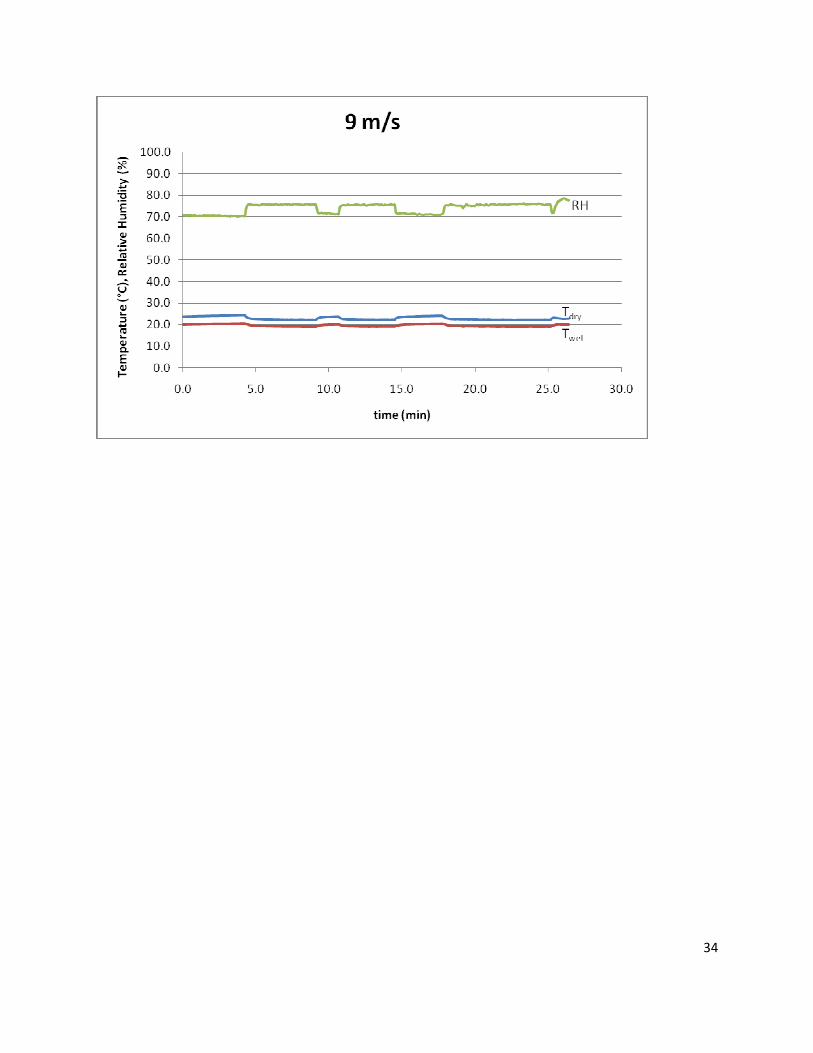
The quality of the air was measured at the outlet using these data loggers for various air

velocities. The following performance curve was obtained. (See Appendix A for graphs detailing

the tests which compose Figure 4.)

15

Figure 4 - Performance curve relating Tdry and RH to air velocity

At a velocity of 4.5 m/s, the relative humidity was roughly 80%.

16

EVAPORATIVE COOLING SYSTEM DESIGN

Design Parameters

As stated in the discussion of the design of the mixing chamber, the evaporative cooling system

was designed to deliver a quasi-uniform mass of air in terms of temperature and relative

humidity. The theoretical expectation for the design was that a control volume (in the present

case, a cold storage room) would eventually be in equilibrium with the incoming air. Once the

point of equilibrium was reached, it was postulated that the humidifying system would maintain

the temperature and relative humidity at a relatively constant level.

Simply providing moisture to a control volume will provide a certain amount of cooling but only

in a batch process: after saturation conditions are reached, no further cooling can be provided and

the temperature will increase due to heat influx from the higher temperature ambient

surroundings. For this reason, it was decided to provide an air flow

Evaporative Cooling Design Set-Up:

The set-up consisted of the following components:

- humidifying unit (MDFD-1)

- mixing chamber

- blower

- delivery pipe

- insulating foam to insulate door opening

- cold storage room at Bioresource Engineering Machine Shop

A representational model can be found in Appendix B which was created with Solid Works 3-D

modelling software. This model does not reflect exact dimensions as some of the features are

extremely difficult to model (i.e. the blower and the contours of the humidifier); because this is

not a working model which is to be tested within the framework of Solid Works itself, it was

decided to forego such detail.

As evaporative cooling works by removing heat from warm, dry ambient air to evaporate water

inside a control volume, the cooling system was placed outside the cold storage room for access

to the ambient air. For previous humidity control experiments, a delivery inlet had been placed

in one of the walls of the cold room (See Figure 5). The inlet’s diameter was a convenient

17

dimension for the delivery pipe of this design, however it was difficult to access because of

space restrictions in the antechamber (which was acting as a storage room) to the cold room. In

order to overcome the challenge in accessing the delivery inlet, objects (such as a filing cabinet

and fridge) were rearranged in the antechamber to facilitate proper spacing and direction for the

evaporative cooling system. It is important to mention that these objects were not part of the

initial design of the delivery apparatus. Unfortunately the physical design of the prototype

evaporative cooler in this design was limited by space and budget. However, pursuant to this

section is a suggested apparatus which will better suit most implementations in terms of space

and budget.

Testing Procedure of Evaporative Cooling Unit

First Testing Setup

Figure 5 - First Setup: Humidifying unit outside control volume

Tests were previously performed to ascertain the performance curve of the delivery system in

terms of minimum temperature obtained and maximum relative humidity of the inlet (to the

control volume) air (See section entitled “Testing of Mixing Chamber”). The next step was to

apply the overall set-up to the cold storage room to verify the hypotheses on humidification and

cooling that were anticipated. These hypotheses related directly to the performance curve

information (See Figure 4) as well as theoretical calculations based on psychrometric principles

(See Appendix F).

In order to determine whether or not the set-up was effective or not, a threshold time value of

approximately one day was chosen as the limit for time to observe cooling and humidifying

effects and more importantly the stabilization of these effects.

18

The first test was run over a period of approximately 24 hours beginning on March 10, 2008

from approximately 15h00 to March 11, 2008 at 15h00. This test was run as a preliminary test in

order to observe the general effects upon the quality of the air in the control room. A replicate

test was run to verify these results beginning March 12, 2008 and ending March 23, 2008.

The parameters of this test were:

- full-time functioning of MDFD-1 unit

o humidity control unit set to 100% RH and 5% variation

- air inlet velocity of approximately 2.5 m/s

- air inlet quality consisted of Tdry, min = 19.5°C, and RHmax = 94%

- a small outlet was cut in the foam at the door to allow air to exit and reduce pressure

build-up within the control volume

The expected end quality of the air was to be in equilibrium with the inlet air and be at a Tdry =

19.5 and RH = 94%. What was observed at the end of the trial period (24 hours later) was much

different from the expected results. Based on the Tdry and Twet readings, Relative Humidity was

calculated using the method stipulated in Appendix X.

Dry-bulb temperature throughout this experiment did not drop as expected to 19.5°C as was

being supplied. As can be seen in Figure X below, Tdry,CV hovered between 22°C and 25°C

throughout the entire experiment. There are a number of explanations for why the temperature

did not drop as expected which follow the presentation of the graphs: fluctuation of ambient air

temperatures, adiabatic nature of the cold-storage room, thermal load, and finally a flawed setup.

The results of the experiment yielded an increase in relative humidity to approximately 80% as

shown in Figure 6. This part of the result can essentially be discarded because the method of

measuring relative humidity relied partly on wet-bulb temperature measurements which were

deemed inaccurate as discussed previously in the section detailing the performance curve

derivation.

19

Figure 6 - Relative Humidity, Tdry,CV vs. time with unit outside control volume

Figure 7 - Tdry,ambient vs. time for unit outside control volume

20

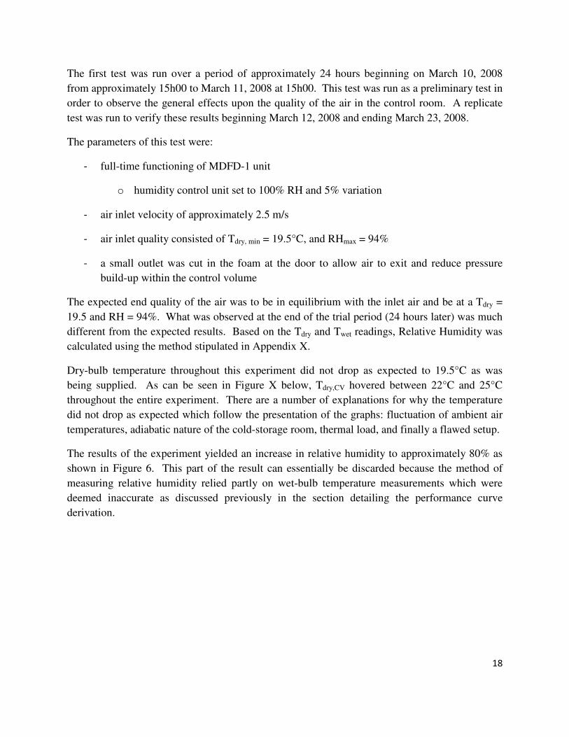
Figure 8 – Tdry,ambient – Tdry,CV vs. time for unit outside control volume

Temperature fluctuations:

As shown in Figure X above, Tdry,ambient fluctuates greatly as it ranges between approximatley

22°C and 33°C. The system relies on humidifying and cooling ambient air which is then input

into the control volume; it logically follows that as the ambient air warms and cools, the inlet air

and consequently the control volume should warm and cool accordingly. In this experiment the

previous statement is not accurate because the temperature of the control volume varies only

slightly, though it does match the pattern of the ambient air fluctuations. This is apparent when

attempting to remove the “noise” (i.e. ambient temperature fluctuations) to prove the

effectiveness of the cooling system. In an effective system, the difference between ambient

temperatures and control volume temperatures is expected to be relatively stable; however, in the

case of this test the difference between the two temperatures has a very unstable, tooth-like

shape.

Adiabatic cold-storage room:

The adiabatic nature of the cold-storage room is significant enough to resist changes to

temperature as it presents a significant barrier between ambient conditions and control volume

conditions. In non-adiabatic conditions, the control volume is somewhat transparent to the

effects of ambient conditions and will consequently be influenced by said conditions. In this

case, the cold-storage room is designed to effectively limit heat entrance and thus maintain stable

temperatures.

21

Thermal Load:

After the first day long test was performed, very little cooling of the control volume air was

observed. Part of the resistance to temperature change can be related to the large thermal mass

that was within the cold storage room; the thermal mass was in the mostly in the form of PVC

pipe sections but also some other miscellaneous articles (eg. wood chair, plastic tubing, foam).

To obtain cooling from this system, it is important to recognize the system in its entirety. More

plainly stated the evaporative cooling system must be concerned with cooling the mass inside the

room as well as the air.

The cold room is designed to be (more or less) an adiabatic unit, but for the purposes of cooling

its inside it cannot be considered an adiabatic system. There is a transfer of heat between the

components inside the cold storage room: air, water, and objects. To simplify the system, the

interactions can be broken up into two sections: i) air-water, and ii) air-objects. While this may

not be an exact reflection of what is occurring, it does allow some analysis. In separating the

interactions in this fashion, it is possible to derive an approximation for how much heat energy

the thermal mass is supplying to the air. Because the driving force of heat transfer is a heat

gradient – such as in Newton’s Law of Cooling (Q = hA[Ts-T∞]) or a thermodynamic analysis (Q

= mcp[T2-T1])- as the air in the control volume is cooled by transferring its heat energy to the

water supplied by the humidified air stream, a temperature gradient between the air and the

thermal mass is created. Consequently, the thermal mass loses heat to the air and the

temperature of the air rises in response. In effect, the supplied moisture must cool both the air

and the thermal mass in the control volume.

It is postulated that the thermal load within the cold storage room was too significant for the

evaporative cooling system. (See Appendix X for an analysis.) The results of this analysis show

that cooling the thermal mass requires 6 times as much energy as cooling the air within the same

cold-storage room. This enhanced energy requirement may play a significant role in limiting

overall temperature drop as well as rates of temperature drop.

Note: The thermal mass is estimated to be wholly due to the PVC pipe sections based on visual

approximation.

Flawed setup:

The setup used was conceived to obtain constant, equilibrium temperature and humidity

conditions. The principle idea was that if cool, humid air was supplied to the control volume at

higher inlet flow rates than was allowed to exit, then the temperature and humidity conditions

would reach an equilibrium – the inlet conditions. However, this setup proved insufficient as

shown by the results. One explanation for poor results based on setup can be related to the

principles behind evaporative cooling. In this setup, ambient air is being cooled and supplied to

the control volume which does not directly remove heat energy from the control volume itself.

22

The more effective setup (discussed in the next section) is to supply the moisture directly to the

control volume air itself, which removes heat energy from the air in the control volume; thus, the

air is cooled directly.

Second Testing Set-Up

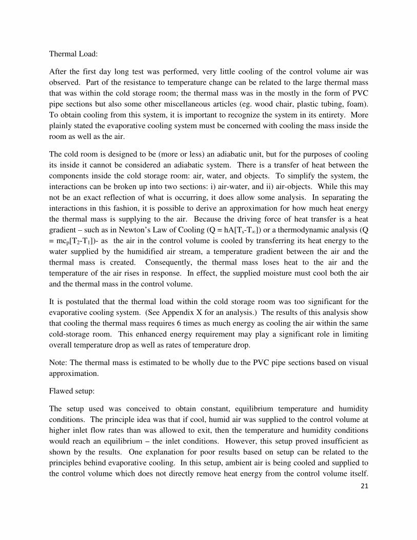
Figure 9 - Second Setup: Humidifying unit inside control volume

As very little cooling was observed over the course of the first testing procedure, it was decided

to place the humidifying unit within the cold-storage room for the same time duration. This

second test was designed to provide a more direct contact application between the water from the

humidifier stream and the air contained in the control volume. The intention was to derive a

more rapid cooling effect from this initial contact.

This second test was run over the course of approximately a 24-hr period beginning at 15h30 on

March 13, 2008 and ending at 15h30 on March 14, 2008. The setup parameters of this test were

as follows:

- control unit of MDFD-1 set to target 100% RH with 5% variability in sensing

o chosen to obtain maximum humidity and temperature drop.

- delivery system was removed (i.e. blower and delivery pipe) although fan was left to

provide air flow for continuous cooling.

- control volume was sealed to limit entrance of warm air.

In this scenario, the relative humidity was expected to near or attain 100%. Based on experience

with the previous test, a final temperature was not forecasted. Although, under normal

conditions, where the intial Tdry,CV and relative humidity were 24°C and 20% respectively, the

23

anticipated Tdry,CV (at near 100% RH) would approach 10°C (See Appendix). The purpose of

this test was to find the final minimum Tdry,CV.

Results:

The Tdry,CV obtained temperatures lower than in the first testing procedure where it was measured

between 18.5°C and 22°C as shown in Figure X. Also in this figure, the relative humidity

reached very high levels as shown by attaining 100% RH for extended periods of time. There

was a problem with this setup however as the humidity control unit was set to 100% RH.

Having the threshold value set this high enabled the humidifying unit to continuously supply

water to the control volume. The problem occurred when the control volume air became

saturated however the unit kept supplying water at which point condensation occurred. When

the test was ended, upon entry to the cold-storage room significant condensation was found on

the floor directly beneath the humidifying unit. The condensation was an indication of a flawed

setup insofar as the humidity control unit was set too high.

Figure 10 – Tdry,CV vs. time with unit inside control volume

24

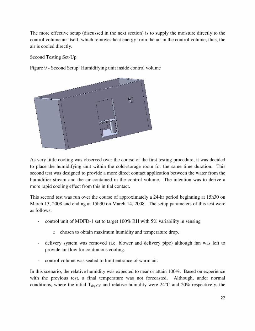
Figure 11 – Tdry,ambient vs. time for unit inside control volume*

Figure 12 - Tdry,ambient – Tdry,CV vs. time with unit inside control volume*

*A discussion of the above two graphs is not necessary given the discussion of the initial test

setup.

25

EVAPORATIVE COOLING EFFECTS ON PRODUCE

The following product quality test was a measure of how well the humidifying unit dispersed

humidity. More specifically, this test allowed some quantification of the effect of that this unit

had on product mass loss. Three different kinds of produce were tested: carrots, radish, and

spinach. Mass measurements were taken at the beginning of the test and at every 24 hour interval

after that. A control test was done for ambient conditions. Due to time constraints however, the

test could not be tested for a period longer than 4 days. The results are presented in the following

table and will be compared a similar experiment conducted by Dadhich et al. (2008).

Table 1 – Overall Percent Weight (%) loss of produce after 4 days

Product Inside C.V Outside C.V

Carrots 21.4% 57.3%

Spinach 40.8% 78.1%

Radish 30.2% 85.1%

At one point during the experiment, the water delivery system malfunctioned and it did not

provide a sufficient amount of water to the humidifier. As a result, the relative humidity inside

the control volume dipped well below 90%. The graph on the following page shows the relative

humidity versus time inside the control volume and exactly at what point during the experiment

this dip in relative humidity occurred. In order to minimize the error from this drop in relative

humidity, the values for percentage mass weight loss during this dip in relative humidity were

interpolated from other mass weight loss values.

26

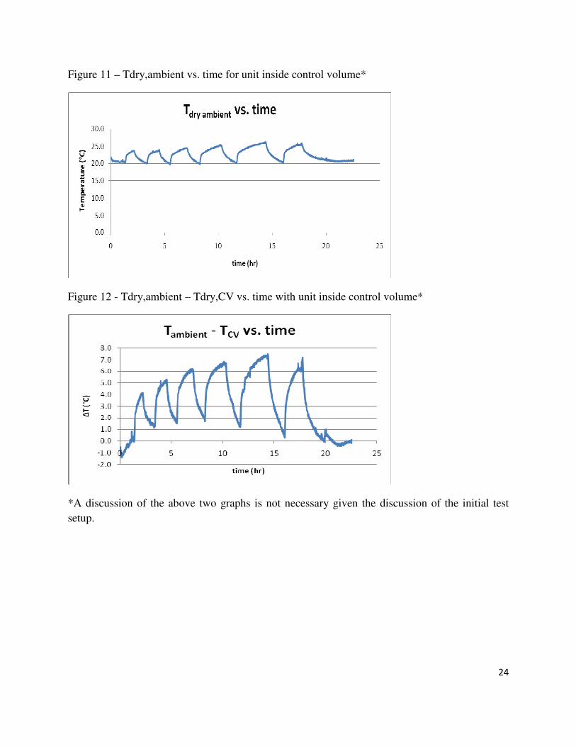
Figure 13 - RH and Tdry inside control volume vs. time

RH and Temp. inside C.V vs Time

0

20

40

60

80

100

120

0 10 20 30 40 50 60 70 80 90 100

time(h)

RH

(%)

From Figure 13, the dip occurred during day 3 interval. So the mass loss values measure for day

3 will be replaced with interpolated values based on day 2 and day 4 measurements. The ambient

conditions are also important to consider and note. The following graph illustrates both the

temperature and the relative humidity of the ambient air.

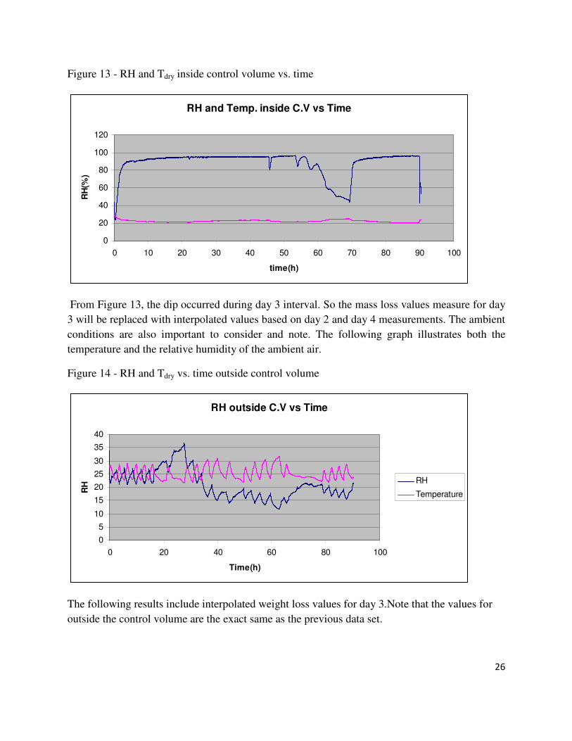
Figure 14 - RH and Tdry vs. time outside control volume

RH outside C.V vs Time

0

5

10

15

20

25

30

35

40

0 20 40 60 80 100

Time(h)

RH

RH

Temperature

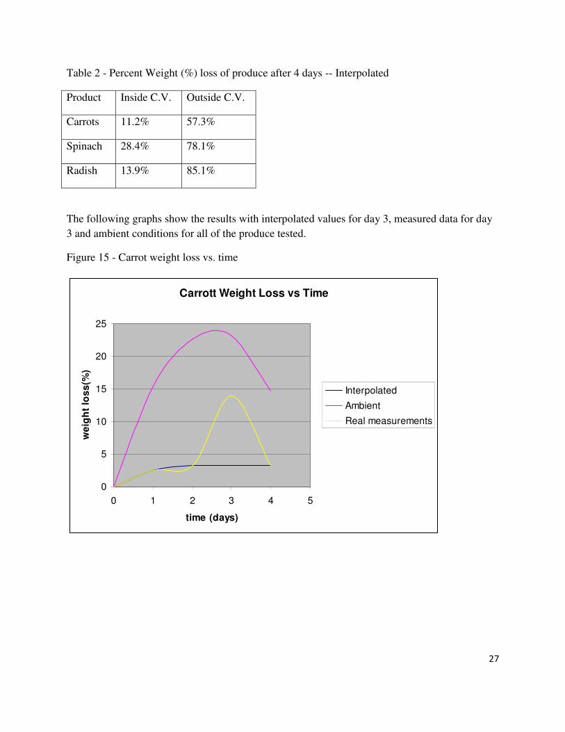
The following results include interpolated weight loss values for day 3.Note that the values for

outside the control volume are the exact same as the previous data set.

27

Table 2 - Percent Weight (%) loss of produce after 4 days -- Interpolated

Product Inside C.V. Outside C.V.

Carrots 11.2% 57.3%

Spinach 28.4% 78.1%

Radish 13.9% 85.1%

The following graphs show the results with interpolated values for day 3, measured data for day

3 and ambient conditions for all of the produce tested.

Figure 15 - Carrot weight loss vs. time

Carrott Weight Loss vs Time

0

5

10

15

20

25

0 1 2 3 4 5

time (days)

we

igh

t lo

ss

(%)

Interpolated

Ambient

Real measurements

28

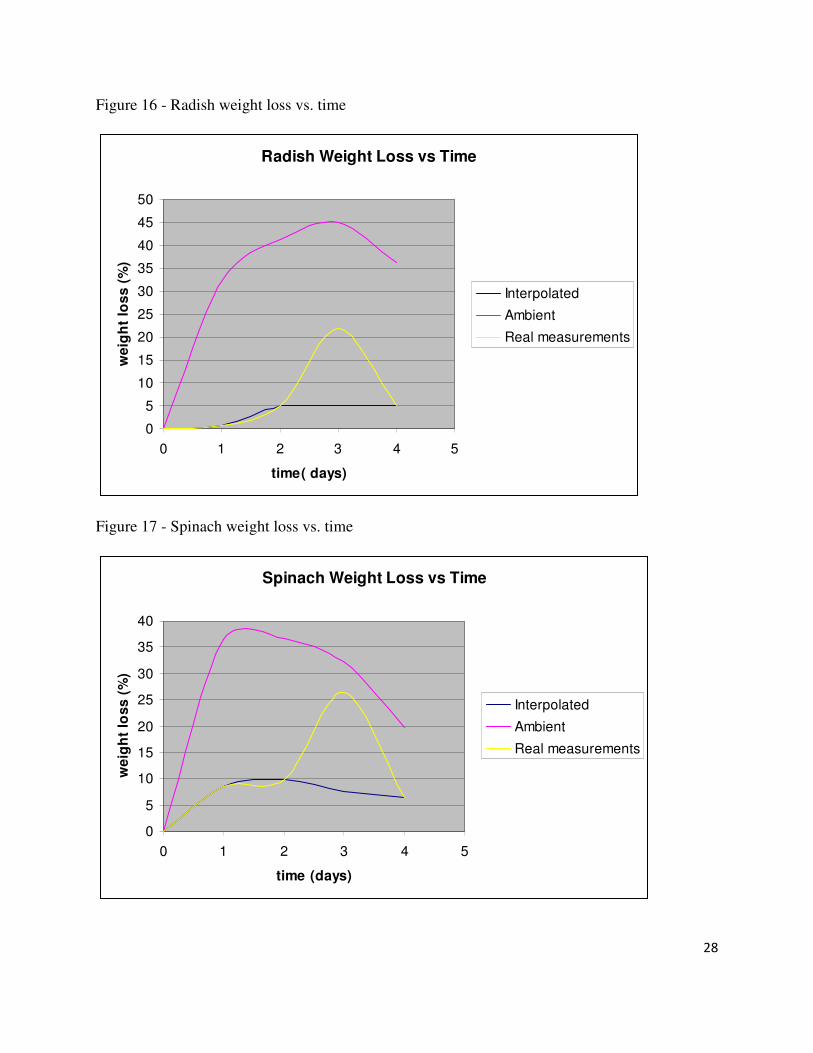
Figure 16 - Radish weight loss vs. time

Radish Weight Loss vs Time

0

5

10

15

20

25

30

35

40

45

50

0 1 2 3 4 5

time( days)

we

igh

t lo

ss

(%

)

Interpolated

Ambient

Real measurements

Figure 17 - Spinach weight loss vs. time

Spinach Weight Loss vs Time

0

5

10

15

20

25

30

35

40

0 1 2 3 4 5

time (days)

we

igh

t lo

ss

(%

)

Interpolated

Ambient

Real measurements

29

The interpreted results might in fact not necessarily reduce the error of the change in relative

humidity inside the control volume. The real measurements and ambient measurements of all the

produce have similar concave shapes that peak around the same point in time. However, the only

precise way to settle any uncertainty in the results and their interpretation is to simply conduct

another test. However, due to time constraints this is not possible.

The results from a similar evaporative cooling experiment by Dadhich et al. (2008) are presented

in the following table.

Table 3 - Percent Weight (%) loss of produce after 7 days

Product Inside C.V Outside C.V

Carrots 5% 50%

Spinach 8% 49%

Radish 12% 55%

These values are weight loss values are considerably lower than the weight loss obtained in the

present experiment. In fact, in Dadhich et al. (2008) the weight losses are for 7 days of storage as

opposed to only 4. However, it must be noted that the experiments were not the same. The first

major source of error to consider would be difference in ambient conditions and in ambient

weight loss. The ambient temperatures in Dadhich et al. (2008) experiment varied from 12°C to

23°C while the ambient temperature in our experiment varied from 23°C to 31°C. Furthermore,

the ambient relative humidity varied from 45% to 60% while for our experiment it varied from

12% to 37%. Therefore, the ambient conditions in our experiment were considerably dryer and

warmer than for Dadhich et al. (2008). In a dryer and warmer environment, moisture loss is

greater. In addition, the conditions inside the control volume are different for both experiments.

The relative humidity is however practically the same but the dry bulb temperatures are quite

different. In our experiment the temperature ranged from 24°C to 20°C while for their

experiment it ranged from 12°C to 23°C. Again, for higher temperatures, moisture loss is greater.

However, it remains uncertain as to whether these differences in temperatures and relative

humidity could result in the considerable difference in percent moisture loss values measured.

One possible source of error in the values that should be noted is the fact that when the produce

was initially massed, there was a considerable amount of moisture on the surfaces of the

vegetables. Perhaps, a more conservative approach would have been to let the surface moisture

dissipate before initial mass measurements were taken.

30

LIMITATIONS AND SETBACKS

This project was fraught with setbacks of all kinds rooted in a number of different causes. Some

of the setbacks resulted from lack of knowledge and experience (ex. wet-bulb thermometer

inaccuracy, oversaturation, etc.) whereas others were a result of equipment failure (ex.

humidifier fan burn-out, water delivery system malfunction, etc.) or time and budget constraints.

This statement is included in order to show that more time would allow for more complete

examination of the evaporative cooling effects that were attempted to be demonstrated.

CONCLUSIONS

In conclusion, the ultrasonic unit exerted a very small cooling effect when integrated into an

evaporative cooling system. It is hypothesised that the reason why the evaporative system did not

cool significantly was due to the high thermal load in the system. Another test could be run with

a reduced thermal load to verify whether this is really the case; however, such a test would most

likely not reflect conditions (notably a fairly high thermal load) found in commercial storage.

Furthermore, quantifying the cooling effect of the unit for commercial storage is one the

objectives of this design project. In addition, the use of a mixing chamber seemed to have very

little effect on the amount of cooling occurring inside the control volume. Finally, the percentage

weight loss results, when compared to the experiments conducted by Dadhich et al. (2008) were

high. However, to properly compare weight loss values to another experiment, all of the testing

environments should be the same. In the test conducted in this design project, both the ambient

and control volume temperatures were significantly higher than that of Dadhich et al. (2008). In

addition, the relative humidity in the ambient conditions was also significantly higher in the

Dadhich et al. (2008). Finally, to truly examine the value of the ultrasonic unit as a humidity

source, and to quantify its effect of produce weight loss, the relative humidity and dry bulb

temperature in the control volume should reflect and simulate the relative humidity and dry bulb

temperature in a commercial storage environment and not that of a warm dry machine shop.

31

REFERENCES

Bartlo, J. 1997. A Wet-Bulb Temperature Equation. A website detailing an accurate method for

determining relative humidity and dew point temperature from Tdry and Twet. Retrieved on March

5, 2008 from http://joseph-bartlo.net/articles/070297.htm.

Bhowmic, S. R., Pan, P. C. 1992 Shelf life of mature green tomatoes stored in controlled

atmosphere and high humidity. Journal of Food Science. 4; 948- 953.

Dadhich, M. S., Dadhich, H., Verma, R. C. 2008. Comparative Study on Storage of Fruits and Vegetables

in Evaporative Cool Chamber and in Ambient. International Journal of Food Engineering. 4(1); 1-

11

DeEll JR, Prange RK, Peppelenbos HW. 2003. Postharvest Physiology of Fresh Fruits and

Vegetables. In: Chakraverty A, Mujumdar AS, Raghavan VGS, Ramaswamy HS, editors.

Handbook of Postharvest Technology. New York (NY): Marcel Dekker, Inc; 455-483.

gorhamschaffler.com. 2008. A website detailing a method used to find relative humidity and other

psychrometric properties. Retrieved on March 5, 2008 from address:

http://www.gorhamschaffler.com/humidity_formulas.htm

Johnson, D. M. 2004. An Evaporative Cooling Model for Teaching Applied Psychrometrics. Journal of

Natural Resources and Life Sciences Education. 33; 121-123.

Mordi, J.I., Olorunda, A.O. 2003. Effect of Evaporative Cooler Environment on the Visual

Qualities and Storage Life of Fresh Tomatoes. Journal of Food Science Technology 40(6): 587-

591.

International Rice Commission. 2002. Issues and Challenges in Rice Technological Development for

Sustainable Food Security. Keynote Address: Twentieth Session. IRC: 02/05.

Narayanasamy P. 2006. Postharvest Pathogens and Disease Management. Hoboken (NJ): John Wiley &

Sons

Thiagu, R., Chand, N., Habibunnisa, E. A., Prasad, B. A., Ramana, K.V.R. 1990. Effect of Evaporative

Cooling Storage on Ripening and Quality of Tomato. Journal of Food Quality. 14; 127-144.

United Nations. 2008. The World at Six Billion. A report from the United Nations regarding population

dynamics in the future. Retrieved on March 20, 2008 from the United Nations Population Division

at http://www.huwu.org/esa/population/publications/sixbillion/sixbilpart1.pdg

Wills R, McGlasson B, Graham D, Joyce D. 2007. Postharvest: An introduction to the

physiology and handling of fruit, vegetables and ornamentals. 5th ed. Cambridge (MA): CABI

32

APPENDIX A – Performance Analysis of Mixing Chamber at Varying Maximum Air

Velocities

Data obtained March 10, 2008.

33

34

35

APPENDIX B – Solid Works Representational Model

The numbers 1 through 6 signify the positions of thermocouples which were used to measure

Tdry (odd) and Twet (even) throughout the experiments.

• 1 and 2 were used to take readings of pre-mixing quality.

• 3 and 4 were used to take readings of post-mixing chamber quality, but pre-blower.

• 5 and 6 were used to take readings of post-mixing and post-blower quality.

• 7 and 8 were used to take reading of ambient air quality.

• 9 and 10 were used to take readings of control volume air quality.

Delivery Pipe

Blower

Foam

Mixing Chamber

Humidifying

Unit

Air Intake

1 2

3 4

5 6

7 8

9

10

Control

Volume

Ambient

36

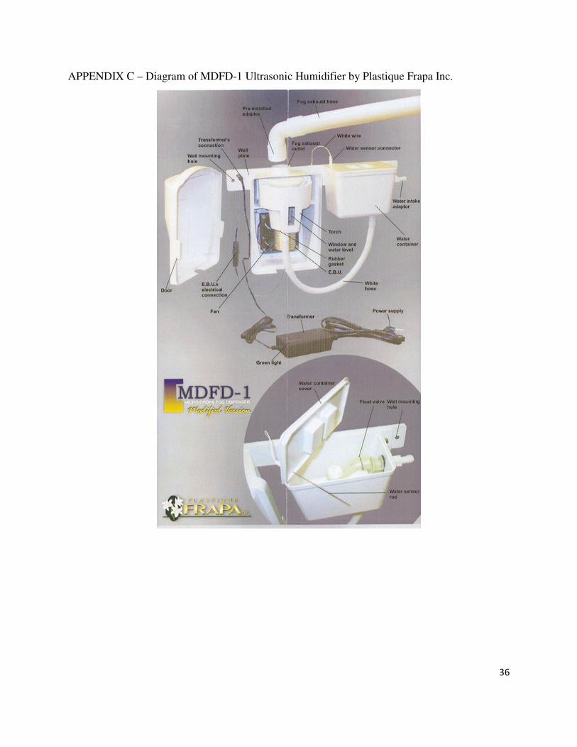
APPENDIX C – Diagram of MDFD-1 Ultrasonic Humidifier by Plastique Frapa Inc.

37

APPENDIX D – Thermal Load Analysis

In this example analysis, the Tdry is assumed to decrease from 22 °C to 15 °C.

• 22 PVC pipe secions

› L = 23” = 0.584 m

› dout = 10-3/4“ = 0.273 m -> rout = 0.1365 m

› din = 9-14/16” = 0.251 m -> rin = 0.1255 m

• 40 PVC pipe caps

› dcap = 9-14/16” = 0.251 m -> rcap = 0.1255 m

› t = 1/4" = 0.00635 m

• ρPVC ≈ 1380 kg·m-3

• cp,PVC ≈ 0.9 kJ·kg-1

·K-1

The equation for heat loss from the pipe to the air will be:

Q = mpipecp,pipe(T2-T1)

Where,

mtotal = Vtotalρ = (aVpipe + bVcaps) ρPVC = [aπ(rout2-rin

2) L + bπrcap

2t]ρPVC = (0.116 +

0.0123)m3·1380 kg·m

-3

= 179.5 kg

NOTE: “a” represents 22 pipe sections and “b” represents 40 pipe caps.

Therefore,

Q = 179.5 kg A 0.9kJ

kg AKffffffffffffffffff

A 7 K = 1130.85 kJ

This analysis in itself is not particularly descriptive and it must be put in relation to the energy

required to cool the air in order to provide perspective.

Again,

Q = mair

cpair

T 2@T 1

b c

Where,

• mair = ρV =1

v

ffff

V =1

0.83m3

kg

ffffffffff

ffffffffffffffffffffffff

A 20.34 m 3= 24.51 kg

38

• cpair

= 1.006kJ

kg AK

fffffffffffffffffff

• Dimensions of control volume: L = 172” = 4.37 m; W = 88” = 2.24 m; H = 83” = 2.08 m

So, over the same temperature drop from 22°C to 15°C,

Q = 24.51 kg A 1.006kJ

kg AKffffffffffffffffff

A 7 K = 172.6 kJ

In comparing this value to the energy required for decreasing the temperature of the PVC piping:

Q

PVC

Qqir

fffffffffffffff

=1130.85 kJ

172.6 kJffffffffffffffffffffffffffffffffff

= 6.55

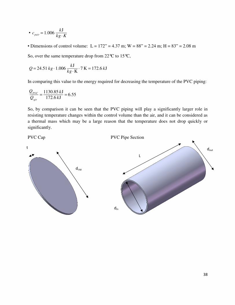
So, by comparison it can be seen that the PVC piping will play a significantly larger role in

resisting temperature changes within the control volume than the air, and it can be considered as

a thermal mass which may be a large reason that the temperature does not drop quickly or

significantly.

PVC Cap PVC Pipe Section

dout

din

L

dcap

t

39

APPENDIX E – Calculation of Relative Humidity from Tdry and Twet

The following method for calculating Relative Humidity was taken from a web article at the

following address: http://joseph-bartlo.net/articles/070297.htm. It was chosen over other

methods because of the accuracy it demonstrated in calculating Relative Humidity.

A number of equations rely on other information regarding the system such as TDP or Humidity

Ration (H) in order to determine RH (gorshamschaffler.com, 2008). Unfortunately, in the

context of this experiment this information is not given and these equations cannot be used.

Even using the equations found in ASHRAE’s Handbook: Principles (ASHRAE, 2005) in the

section concerning psychrometrics, the RH which is calculated is inaccurate.

For example, for the conditions of Tdry = 30°C and Twet = 15°C, using the equations in ASHRAE

(2005) yields a RH = 21%. In contrast, using the method in question which was outlined by Mr.

Joseph Bartlo yields RH = 17.3%. Upon inspection of a psychrometric chart (See Appendix F),

the latter value seems to be very accurate as the intersection point on the chart is approximately

RH = 17.5% (See psychrometric chart in Appendix X).

Description of method:

During the wet-bulb process, air, water and water vapour coexist; some vapour may be

condensed or water may be evaporated into the air, saturating it. These are isobaric processes

where, as water vapour content in the air changes, the air volume also changes. In these

processes, it is the latent heat of vapourization that is responsible for the temperature changes.

The process is governed by the following equation:

(MdCpd + MvCpv) dT = -Lv dMv (1)

Where,

Md = dry air mass

Mv = water vapour mass

Cpd = dry air specific heat, constant pressure

Cpv = water vapour specific heat, constant pressure

Lv = vapourization of latent heat

T = temperature

Dividing (1) by Md gives the following:

(Cpd +RCpv) dT = -Lv dR (2)

Where,

R = Mv/Md, which is recognized as the water vapour mixing ratio.

40

The author isolates dR in (2) and integrates with respect to Tdry and Twet which is very difficult

given that R and Lv are functions of Tdry. As an approximation, the author uses a representative

value for R and Tdry:

R = Rwet + ((Cpd + R”Cpv)/Lv)(Twet-Tdry) (3)

R” = Rwet/2 (4)

T” = (Tdry+Twet)/2 (5)

Lv = 2500800 – 2370 T” (6)

Saturation vapour pressure is given by the Wexler equation as follows:

Es = 6.112 e(17.67 T/(243.5+T))

(7)

And the mixture ratio is related to the vapour pressure by:

R = zE/(P-E) (8)

E =RP/(z+R) (9)

Where,

Z = water vapour molecular mass/ dry air molecular mass = 0.62197

E = water vapour pressure

P = pressure (measured in mbar)

Finally, RH can be found from:

RH = E/Es * 100% (10)

Sample calculation:

Given Tdry = 30°C and Twet = 15°C.

i) Calculate Lv using Twet and (6).

Lv = 2500800 – 2370(15) = 2465250 J

ii) Calculate Es,wet using Twet and (6).

Es,wet = 6.112 e(17.67(15)/(243.5+15))

= 17.04049 Pa

iii) Calculate Rwet using Twet and (8).

Rwet = (0.62917)(18.169)/(1000-18.169) = 0.010782 kg H2O/kg dry air

iv) Find R” using (4).

R” = 0.011510/2 = 0.005391 kg H2O/kg dry air

41

v) Find R using (3) – NOTE: Cpd ≈ 1006.3 J/kg/K and Cpv ≈ 1850 J/kg/K

R = 0.010782 + ((1006.3+(0.005391)(1850)/2465250)(15-30) = 0.004599 kg H2O/kg

dry air

vi) Find E using (9).

E = (0.004599)(1000)/(0.62197 + 0.004599) = 7.339688 Pa

vii) Find Es using Tdry and (6).

Es = 6.112 e(17.67(30)/(243.5+30))

= 42.45575 Pa

viii) Finally, find RH using (10).

RH = (7.339688)/(42.45575) * 100% = 17.28785%

42

APPENDIX F – Daily Weight Loss of Produce

Daily Percent Weight Loss of Carrots

Inside C.V Outside C.V

Day 1 2.6% 15.4%

Day 2 3.3% 22.7%

Day 3 13.9% 23.2%

Day 4 3.3% 14.7%

Daily Percent Weight loss of Spinach

Inside C.V Outside C.V

Day 1 8.5% 36.4%

Day 2 9.9% 36.6%

Day 3 26.4% 32.2%

Day 4 6.5% 19.7%

Daily Percent Weight loss of Radish

Inside C.V Outside C.V

Day 1 0.55% 32.1%

Day 2 5.1% 41.2%

Day 3 22% 45.0%

Day 4 5.2% 36.2%

43

44

APPENDIX G – Psychrometric Chart

45

APPENDIX H - Ideal Mixing Chamber Velocity

The ambient air in testing environment is 25% RH, and dry bulb T of 25 ̊ C. To humidify this air

to 85%, the dry bulb temperature from psychometric chart is 16.5 ̊ C.

-The humidity ratio of initial air (@ 25% RH, and dry bulb T of 25 ̊ C) = 0.0055kg water / kg dry

air.

-The humidity of final air (@ 85% RH, and dry bulb T of 16.5 ̊C) = 0.0095 kg water/ kg dry air.

Therefore, delivery system must add:

0.0095 kgwater

kg dry air

fffffffffffffffffffffffffffffff

@ 0.0055 kgwater

kg dry air

fffffffffffffffffffffffffffffff

= 0.0040 kgwater

kg dry air

fffffffffffffffffffffffffffffff

The average operating amount of water the humidifier adds to the system is 0.5 L/h or

0.5kg / h.

This translates into 1.4 E-4 kg water/h.

# 1.4 E@ 4kg water

h

ffffffffffffffffffffffffffffA

X

fffffff

= 0.0040 kgwater

kg dry air

fffffffffffffffffffffffffffffff

X = 0.035kg air

s

fffffffffffffffffff

= 0.035m 3

s

fffffffff

This assumes an average air density of 1kg

m 3

fffffffff

.

Area of 4 inch pipe used in mixing chamber:

Area = πd

4

4fffffff

= 0.0081 m 2

X

area

ffffffffffffff

= 0.035

m3

s

fffffffff

0.0081fffffffffffffffffffff

m 2= 4.3

m

s

ffffff