Embed Size (px)
Citation preview


1
CIVIL ENGINEERING SERIES Hydraulic Engineering Series No. 104
Numerical Modeling of Selected Sediment Traps in Kalamazoo River, Michigan
Ven Te Chow Hydrosystems Laboratory Civil and Environmental Engineering University of Illinois Urbana, Illinois
ISSN: 0442-1744
Zhenduo Zhu1 Marcelo H. Garcia2
1Graduate Research Assistant 2Professor and Director Ven Te Chow Hydrosystems Laboratory
June 2015
Prepared for: U.S. Environmental Protection Agency Region 5 Chicago, IL 60604-3590
2
Numerical Modeling of Selected Sediment Traps in
Kalamazoo River, Michigan
by
Zhenduo Zhu and Marcelo H. García
Ven Te Chow Hydrosystems Laboratory
Department of Civil and Environmental Engineering
University of Illinois at Urbana and Champaign, IL
3
Table of Contents
Executive Summary ........................................................................................................... 6
1. Introduction .................................................................................................................... 7
2. Description of the Numerical Models ............................................................................ 8
2.1 Computational Meshes............................................................................................. 8
2.2 Bathymetry ............................................................................................................. 10
2.3 Model Scenarios and Boundary Conditions .......................................................... 12
3. Results of MP 10.4&10.5 Sediment Trap Model ......................................................... 17
3.1 Distribution of Depth-Averaged Velocity Magnitude ............................................ 17
3.2 Distribution of Bed Shear Stress ............................................................................ 21
4. Results of MP 14.75 Sediment Trap Model ................................................................. 23
4.1 Distribution of Depth-Averaged Velocity Magnitude ............................................ 23
4.2 Distribution of Bed Shear Stress ............................................................................ 26
4.3 An Example Run of Sediment Transport Simulation (100-year Flood Scenario) . 28
5. Results of MP 21.5 Sediment Trap Model ................................................................... 31
5.1 Distribution of Depth-Averaged Velocity Magnitude ............................................ 31
5.2 Distribution of Bed Shear Stress ............................................................................ 33
6. Summary ...................................................................................................................... 36
Acknowledgments............................................................................................................ 37
Bibliography .................................................................................................................... 38

4
Table of Figures Figure 1. Location of Modeled Sediment Traps ............................................................................. 7
Figure 2. Computational Meshes of MP 10.4&10.5 Sediment Trap .............................................. 9
Figure 3. Computational Meshes of MP 14.75 Sediment Trap ...................................................... 9
Figure 4. Computational Meshes of MP 21.5 Sediment Trap ...................................................... 10
Figure 5. Bed Elevation of River and Floodplain at MP 10.4&10.5 Sediment Trap .................... 11
Figure 6. Bed Elevation of River and Floodplain at MP 14.75 Sediment Trap ............................ 11
Figure 7. Bed Elevation of River and Floodplain at MP 21.5 Sediment Trap .............................. 12
Figure 8. Flow Statistics for the Kalamazoo River at Comstock, MI (based on 1933-2013 data)13
Figure 9. Boundary Conditions of April 9-29, 2013 at MP 10.4&10.5 Sediment Trap ................ 13
Figure 10. Boundary Conditions of July 11-19, 2013 at MP 10.4&10.5 Sediment Trap ............. 14
Figure 11. Boundary Conditions of April 9-29, 2013 at MP 14.75 Sediment Trap ...................... 14
Figure 12. Boundary Conditions of July 11-19, 2013 at MP 14.75 Sediment Trap ..................... 15
Figure 13. Boundary Conditions of April 9-29, 2013 at MP 21.5 Sediment Trap ........................ 15
Figure 14. Boundary Conditions of July 11-19, 2013 at MP 21.5 Sediment Trap ....................... 16
Figure 15. Distribution of Velocity Magnitude (MP10.4&10.5, 20:00 April 13, 2013) ............... 18
Figure 16. Distribution of Velocity Magnitude (MP10.4&10.5, 8:00 April 21, 2013) ................. 18
Figure 17. Distribution of Velocity Magnitude (MP10.4&10.5, 20:00 July 17, 2013) ................ 19
Figure 18. Flow Path and Recirculation Zones (MP10.4&10.5, 8:00 April 21, 2013) ................. 19
Figure 19. Survey of Submerged Oil in the Modeling Domain of MP 10.4&10.5 (figure from the
Enbridge Energy, L.P. report [1]) ................................................................................................. 20
Figure 20. Distribution of Bed Shear Stress (MP10.4&10.5, 20:00 April 13, 2013) ................... 21
Figure 21. Distribution of Bed Shear Stress (MP10.4&10.5, 8:00 April 21, 2013) ..................... 22
Figure 22. Distribution of Bed Shear Stress (MP10.4&10.5, 20:00 July 17, 2013) ..................... 22
Figure 23. Distribution of Velocity Magnitude (MP14.75, 4:00 April 14, 2013) ......................... 23
Figure 24. Distribution of Velocity Magnitude (MP14.75, 12:00 April 21, 2013) ....................... 24
Figure 25. Flow Path at 2nd Bifurcation and Confluence (MP14.75, 0:00 April 20, 2013) .......... 24
Figure 26. Flow Path at 1st Bifurcation and Confluence (MP14.75, 0:00 April 20, 2013) ........... 25
Figure 27. Distribution of Velocity Magnitude (MP14.75, 0:00 July 12, 2013) .......................... 25
Figure 28. Distribution of Bed Shear Stress (MP14.75, 4:00 April 14, 2013) ............................. 27
Figure 29. Distribution of Bed Shear Stress (MP14.75, 12:00 April 21, 2013) ........................... 27
Figure 30. Distribution of Bed Shear Stress (MP14.75, 0:00 July 12, 2013) ............................... 28
Figure 31. Distribution of Velocity Magnitude in 100-year Flood Scenario (MP14.75) .............. 29
Figure 32. Distribution of Bed Shear Stress in 100-year Flood Scenario (MP14.75) .................. 30
Figure 33. Distribution of Suspended Sediment Concentration in 100-year Flood Scenario
(MP14.75)..................................................................................................................................... 30
5
Figure 34. Distribution of Velocity Magnitude (MP21.5, 16:00 April 14, 2013) ......................... 31
Figure 35. Distribution of Velocity Magnitude (MP21.5, 16:00 April 21, 2013) ......................... 32
Figure 36. Distribution of Velocity Magnitude (MP21.5, 8:00 July 16, 2013) ............................ 32
Figure 37. Distribution of Bed Shear Stress (MP21.5, 16:00 April 14, 2013) ............................. 33
Figure 38. Distribution of Bed Shear Stress (MP21.5, 16:00 April 21, 2013) ............................. 34
Figure 39. Distribution of Bed Shear Stress (MP21.5, 8:00 July 16, 2013) ................................. 34
Figure 40. Survey of Submerged Oil in the Modeling Domain of MP 21.5 (figure from the
Enbridge Energy, L.P. report [1]) ................................................................................................. 35

6
Executive Summary
The July 2010 spill of diluted bitumen into the Kalamazoo River was the largest release
of heavy crude into an inland waterway in U.S. history. Since the spill, extensive cleanup
and recovery efforts have taken place. However, substantial residual deposits from the
oil spill remained in the river system due to formation of oil-particle aggregates (OPA)
and their negative buoyancy. It is important to understand the conditions under which
the OPA could be entrained into suspension, transported and re-deposited. An in-house
numerical code, HydroSed2D, was utilized to simulate OPA transport and settling in
selected natural sediment traps (hereafter referred to as sediment traps) along the
Kalamazoo River. The sediment traps were constructed to concentrate and hold
submerged oil in an attempt to prevent it from migrating downstream before it could be
recovered. HydroSed2D program enabled a nested approach with an unstructured mesh
design which provided a higher spatial resolution and afforded a more detailed
morphology of the sediment traps than could be achieved through the 2-D
Environmental Fluid Dynamics Code (EFDC) hydrodynamic and sediment transport
models. The HydroSed2D model complemented the 2-D EFDC models which covered a
much larger numerical domain but had a coarser computational mesh.
Three sediment traps, MP10.4&10.5, MP14.75, and MP21.5, were chosen to be
modeled. Each channel reach had different geomorphic characteristics. It was found that
deposition happened under relatively high flow conditions, when river water would flow
into the sediment traps and OPAs would deposit due to a reduction in sediment transport
capacity associated with low flow velocities and bed shear stresses that were illustrated
by the model. The depositional areas indicated by the models agreed in general with the
mapped areas where heavy submerged oil was found during field assessments. The
models developed during this effort are useful tools in the ongoing cleanup work and
may also be useful for future management efforts associated with oil spill accidents.
7
1. Introduction
Following the oil spill at Kalamazoo River waterways system in 2010, extensive oil
cleanup and environmental remediation efforts have taken place. Sediment traps, e.g.
cutoff channel and meanders, are very critical areas for the cleanup work and future
management because high concentrations of oil-particle aggregates (OPA) have a
tendency to deposit there. This facilitates recovery efforts to remove OPAs from the
river.
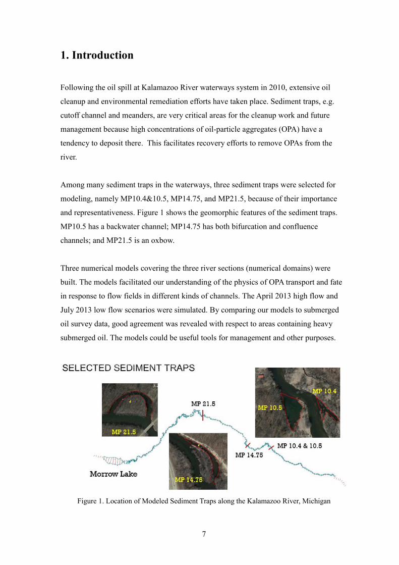
Among many sediment traps in the waterways, three sediment traps were selected for
modeling, namely MP10.4&10.5, MP14.75, and MP21.5, because of their importance
and representativeness. Figure 1 shows the geomorphic features of the sediment traps.
MP10.5 has a backwater channel; MP14.75 has both bifurcation and confluence
channels; and MP21.5 is an oxbow.
Three numerical models covering the three river sections (numerical domains) were
built. The models facilitated our understanding of the physics of OPA transport and fate
in response to flow fields in different kinds of channels. The April 2013 high flow and
July 2013 low flow scenarios were simulated. By comparing our models to submerged
oil survey data, good agreement was revealed with respect to areas containing heavy
submerged oil. The models could be useful tools for management and other purposes.
Figure 1. Location of Modeled Sediment Traps along the Kalamazoo River, Michigan

8
2. Description of the Numerical Models
An in-house code developed at Ven Te Chow Hydrosystems Laboratory, HydroSed2D,
was used in this study. HydroSed2D was developed as a two-dimensional shallow water
model coupled with a bedload sediment transport model (Liu et al. 2008). Zhu (2011)
implemented suspended sediment transport into HydroSed2D. The model has been
tested and applied to many studies and has also helped to understand sediment transport
problems in floodplains and flood control channels (Zhu et al. 2011, Liu et al. 2012, and
Goodwell et al. 2014). The detailed governing equations of HydroSed2D can be found in
Zhu (2011). In this study, the scope of the Hydrosed2D/sediment trap modeling was
limited to the use of the model to simulate hydrodynamic conditions only for two of the
sediment trap areas (e.g., MP10.5 and MP21.5), while the hydrodynamic and sediment
transport simulations were performed for the third area (MP14.75). Manning’s
coefficient n = 0.03 was used as a constant for all three sediment traps.
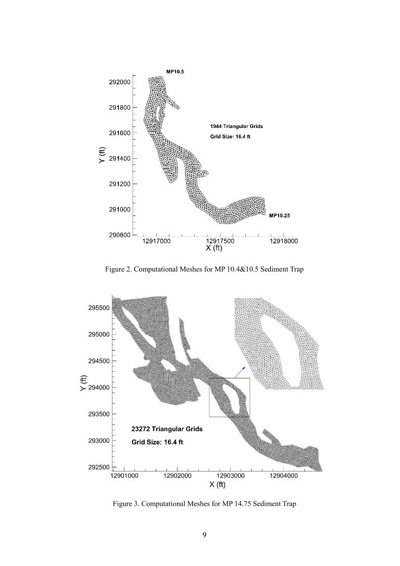
2.1 Computational Meshes
The model used finite volume method and unstructured meshes. Unlike structured
meshes, unstructured triangular meshes allow modelers to deal with complex
geometries. The computational meshes of the three sediment traps are shown in figures 2
to 4. A high degree of spatial resolution was obtained thanks to the use of unstructured
meshes which can adapt to complex morphologies.
9
Figure 2. Computational Meshes for MP 10.4&10.5 Sediment Trap
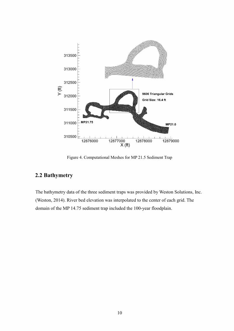
Figure 3. Computational Meshes for MP 14.75 Sediment Trap
10
Figure 4. Computational Meshes for MP 21.5 Sediment Trap
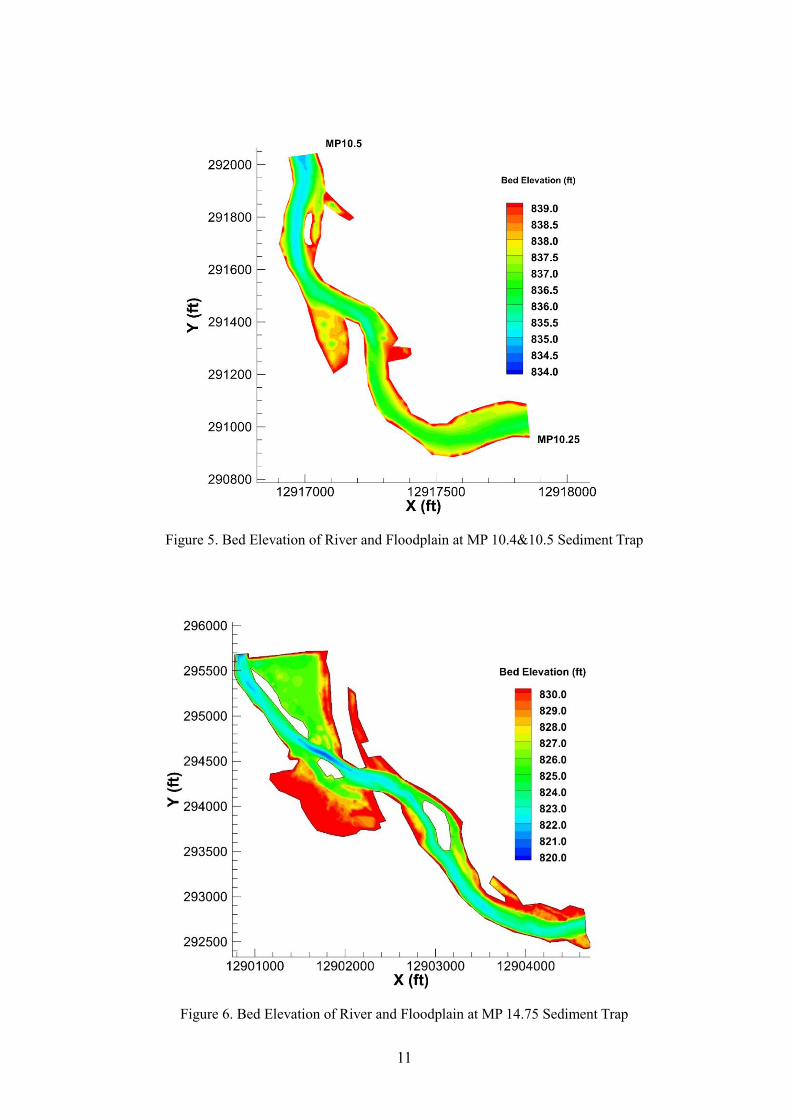
2.2 Bathymetry
The bathymetry data of the three sediment traps was provided by Weston Solutions, Inc.
(Weston, 2014). River bed elevation was interpolated to the center of each grid. The
domain of the MP 14.75 sediment trap included the 100-year floodplain.
11
Figure 5. Bed Elevation of River and Floodplain at MP 10.4&10.5 Sediment Trap
Figure 6. Bed Elevation of River and Floodplain at MP 14.75 Sediment Trap
12
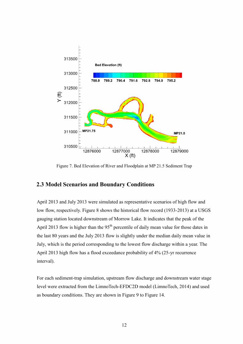
Figure 7. Bed Elevation of River and Floodplain at MP 21.5 Sediment Trap
2.3 Model Scenarios and Boundary Conditions
April 2013 and July 2013 were simulated as representative scenarios of high flow and
low flow, respectively. Figure 8 shows the historical flow record (1933-2013) at a USGS
gauging station located downstream of Morrow Lake. It indicates that the peak of the
April 2013 flow is higher than the 95th percentile of daily mean value for those dates in
the last 80 years and the July 2013 flow is slightly under the median daily mean value in
July, which is the period corresponding to the lowest flow discharge within a year. The
April 2013 high flow has a flood exceedance probability of 4% (25-yr recurrence
interval).
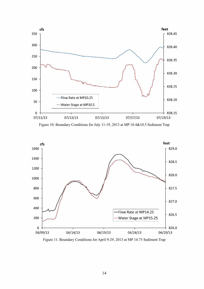
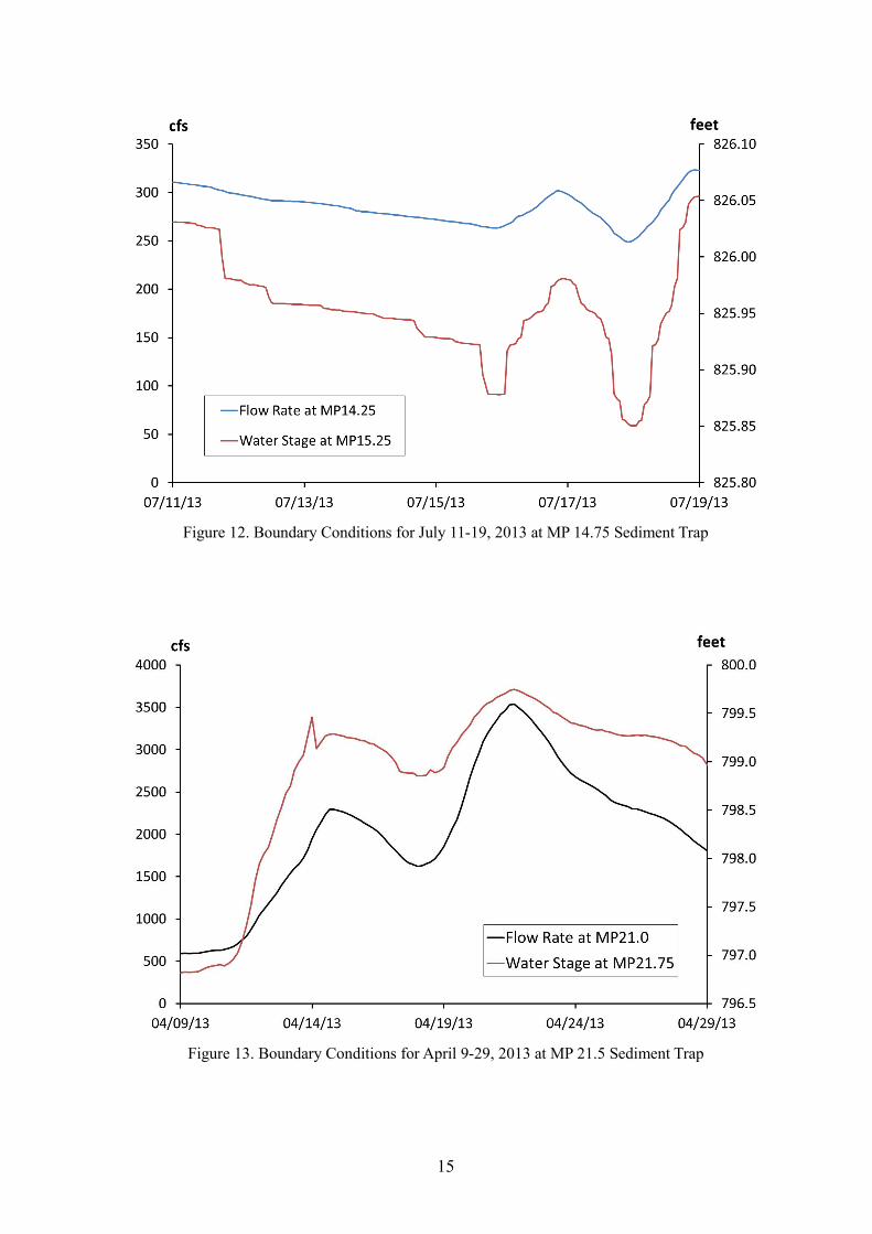
For each sediment-trap simulation, upstream flow discharge and downstream water stage
level were extracted from the LimnoTech-EFDC2D model (LimnoTech, 2014) and used
as boundary conditions. They are shown in Figure 9 to Figure 14.

13
Figure 8. Flow Statistics for the Kalamazoo River at Comstock, MI (based on 1933-2013 data)
Figure 9. Boundary Conditions for April 9-29, 2013 at MP 10.4&10.5 Sediment Trap
14
Figure 10. Boundary Conditions for July 11-19, 2013 at MP 10.4&10.5 Sediment Trap
Figure 11. Boundary Conditions for April 9-29, 2013 at MP 14.75 Sediment Trap
15
Figure 12. Boundary Conditions for July 11-19, 2013 at MP 14.75 Sediment Trap
Figure 13. Boundary Conditions for April 9-29, 2013 at MP 21.5 Sediment Trap

16
Figure 14. Boundary Conditions for July 11-19, 2013 at MP 21.5 Sediment Trap
17
3. Results of MP 10.4&10.5 Sediment Trap Model
3.1 Distribution of Depth-Averaged Velocity Magnitude
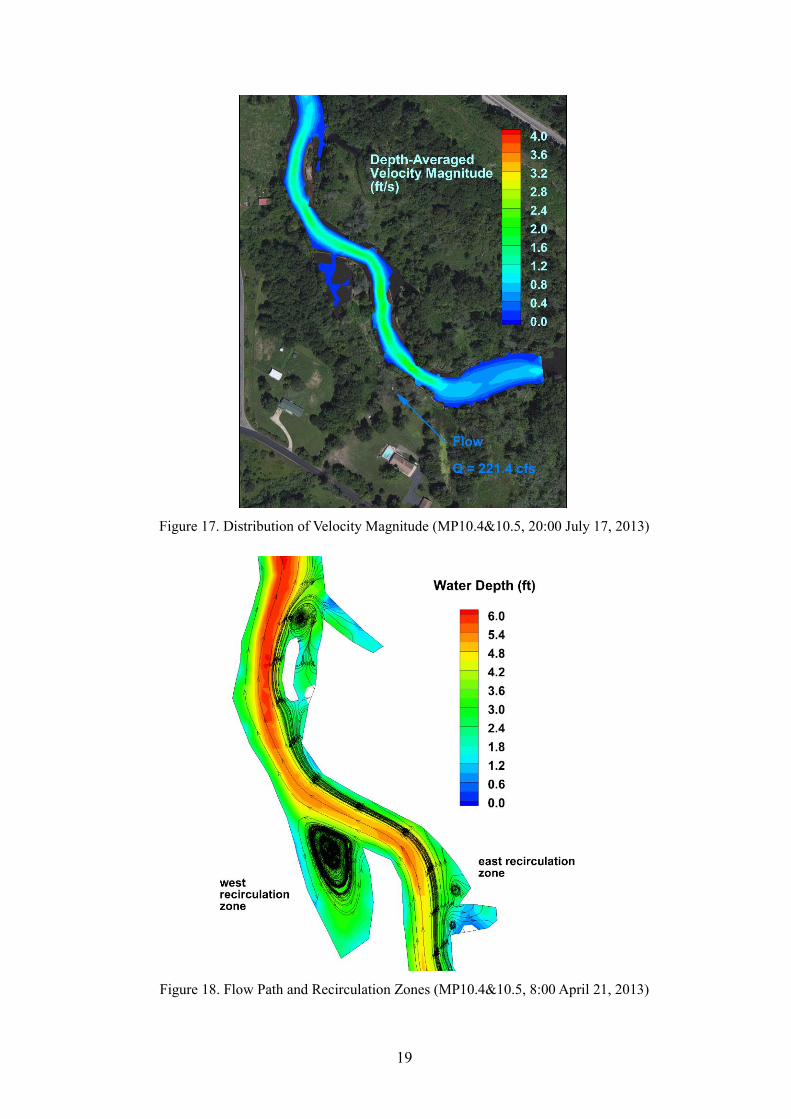
Figure 15, Figure 16, and Figure 17 show examples of the depth-averaged velocity
magnitude in high flow (April 2013) and low flow (July 2013) scenarios. There were
two peaks in the April 2013 scenario (see Figure 9) and both of them are plotted. The dry
water depth was defined as 0.1 meter, i.e. 0.33 ft. Under the high flow conditions, it is
shown that the low velocities are present in the sediment traps MP10.4 and MP10.5.
Also, there is a bifurcation channel along the right descending bank north of the
sediment traps where velocities are low. However, under the low flow condition, water
is constrained in the main channel. The absence of model results shown in the Figure 17
indicates that the simulated water depths were below the minimum model threshold of
10 cm or 0.3 ft. While water below this minimum depth may be present, significant new
contributions of water or sediment to the sediment traps are unlikely under these very
low flow conditions. The simulations showed that flows and therefore OPAs can enter
the trap areas during high flow period and remain there because of the low flow
velocities and bed shear stresses. This suggests that the sediment trap is performing
well.

18
Figure 15. Distribution of Velocity Magnitude (MP10.4&10.5, 20:00 April 13, 2013)
Figure 16. Distribution of Velocity Magnitude (MP10.4&10.5, 8:00 April 21, 2013)
19
Figure 17. Distribution of Velocity Magnitude (MP10.4&10.5, 20:00 July 17, 2013)
Figure 18. Flow Path and Recirculation Zones (MP10.4&10.5, 8:00 April 21, 2013)

20
Figure 19. Survey of Submerged Oil in the Modeling Domain of MP 10.4&10.5 (figure from the
Enbridge Energy, L.P. report [1])
The deposition areas according to field poling results in this domain are shown in Figure
19. The poling results show a qualitative description of oiled sediment as heavy (red),
moderate (orange), light (yellow), and none (blue) in the sediment traps modeled at MP
10.5 site. The reason for deposition is flow recirculation and the loss of sediment
transport capacity. The OPAs enter recirculation zones where flow velocities are so small
that the flow cannot keep OPAs in suspension. Moreover, recirculation of flow does not
allow OPAs to move out of those zones so eventually they end up depositing. Figure 18
shows the flow path of the numerical simulation.
Once the OPAs are entrained into the recirculation zone, the majority are expected to
deposit before being re-entrained into the main channel. The west recirculation zone (see
Figure 18) could be easily recognized. The east recirculation zone also has the potential
to be net depositional. It is also noted that there is another recirculation zone
downstream which indicates possible deposition of OPAs.
21
3.2 Distribution of Bed Shear Stress
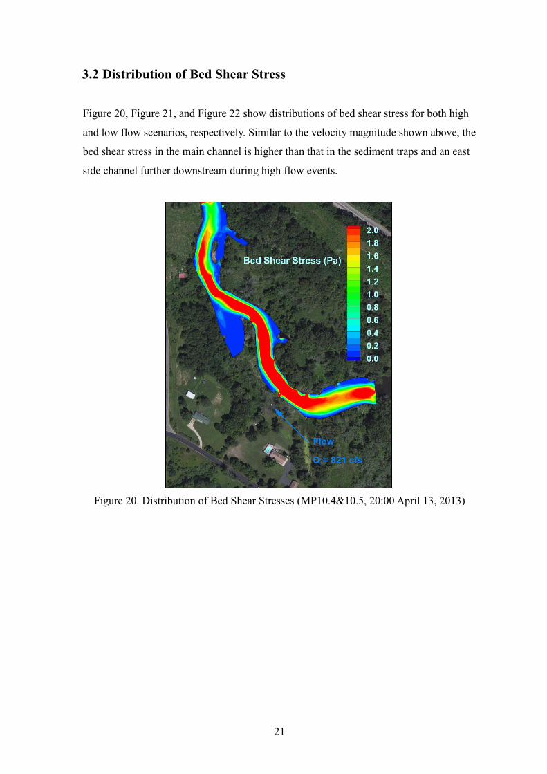
Figure 20, Figure 21, and Figure 22 show distributions of bed shear stress for both high
and low flow scenarios, respectively. Similar to the velocity magnitude shown above, the
bed shear stress in the main channel is higher than that in the sediment traps and an east
side channel further downstream during high flow events.
Figure 20. Distribution of Bed Shear Stresses (MP10.4&10.5, 20:00 April 13, 2013)

22
Figure 21. Distribution of Bed Shear Stresses (MP10.4&10.5, 8:00 April 21, 2013)
Figure 22. Distribution of Bed Shear Stresses (MP10.4&10.5, 20:00 July 17, 2013)
23
4. Results of MP 14.75 Sediment Trap Model
4.1 Distribution of Depth-Averaged Velocity Magnitude
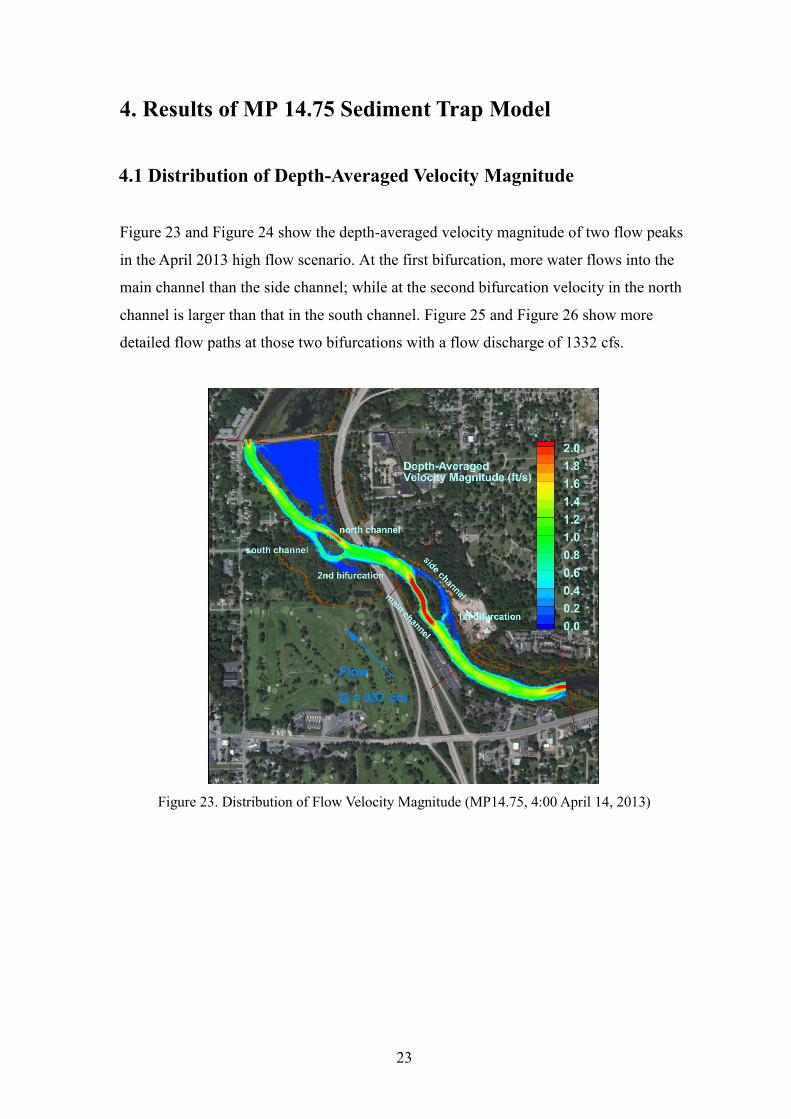
Figure 23 and Figure 24 show the depth-averaged velocity magnitude of two flow peaks
in the April 2013 high flow scenario. At the first bifurcation, more water flows into the
main channel than the side channel; while at the second bifurcation velocity in the north
channel is larger than that in the south channel. Figure 25 and Figure 26 show more
detailed flow paths at those two bifurcations with a flow discharge of 1332 cfs.
Figure 23. Distribution of Flow Velocity Magnitude (MP14.75, 4:00 April 14, 2013)

24
Figure 24. Distribution of Flow Velocity Magnitude (MP14.75, 12:00 April 21, 2013)
Figure 25. Flow Paths at 2nd Bifurcation and Confluence (MP14.75, 0:00 April 20, 2013)

25
Figure 26. Flow Paths at 1st Bifurcation and Confluence (MP14.75, 0:00 April 20, 2013)
Figure 27. Distribution of Velocity Magnitude (MP14.75, 0:00 July 12, 2013)
Figure 27 shows an example of the velocity distribution in the July 2013 low flow
scenario. The discharge was 298 cfs at 0:00 in July 12, 2013. The difference between the
velocity magnitude and inundation areas between the two scenarios is evident.
HydroSed2D model is capable of simulating wetting and drying automatically. The

26
important characteristic of this sediment trap is the channel bifurcation, where the flow
separates, and the confluence where the separated flows join again. Sediment deposition
and erosion occurs due to the distribution of flow discharge and the change in flow
velocities as well as bed shear stresses.
During low flows, the flow follows the main channel only, so that no water and sediment
can flow into the bifurcation channel. Also, the sediment load is usually so low that not
much morphological change happens. However, high flows can cause significant
transport of sediment.
Figure 24 shows that at the first bifurcation more water flows through the main channel
than along the side channel. Flow velocities and bed shear stress are much lower in the
side channel (see Figure 29). Sediment can be expected to deposit due to reduced flow
velocity and associated gradient in bed shear stresses and reduction in sediment transport
capacity. At the second bifurcation, more water flows into the north channel, but the
south channel flow velocity is not reduced as much as in the first bifurcation. There is a
low-velocity zone at the confluence where sediment may deposit. Also, there is a “dead
zone” at the south end of the south bifurcation channel which is also a potential
depositional area. Immediately after the second confluence, there is another small side
channel which bypasses some of the flow into a large floodplain, where deposition can
be expected to occur due to much lower velocities.
4.2 Distribution of Bed Shear Stress
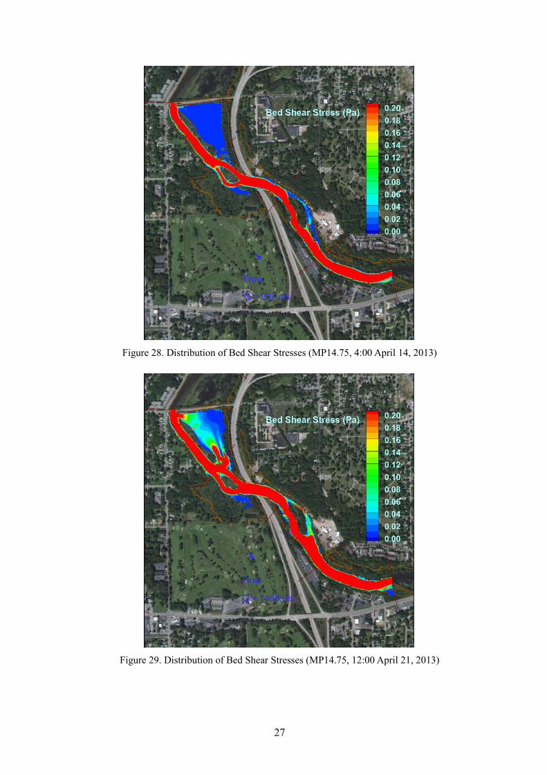
Similarly to the above depth-averaged velocity plots, Figure 28, Figure 29, and Figure
30 show distributions of bed shear stress in high and low flow scenarios.
Bed shear stress provides patterns similar to those for velocity magnitude in terms of
distribution. Moreover, bed shear stress is a better indicator for sediment transport,
especially the fate and transport of oil-particle aggregates (OPAs). In-situ flume and lab
experiments suggest that the critical bed shear stress for OPA resuspension may be as
low as 0.1 Pa. The areas with less than 0.1 Pa bed shear stresses are most likely areas
with large concentrations of submerged oiled sediments.
27
Figure 28. Distribution of Bed Shear Stresses (MP14.75, 4:00 April 14, 2013)
Figure 29. Distribution of Bed Shear Stresses (MP14.75, 12:00 April 21, 2013)
28
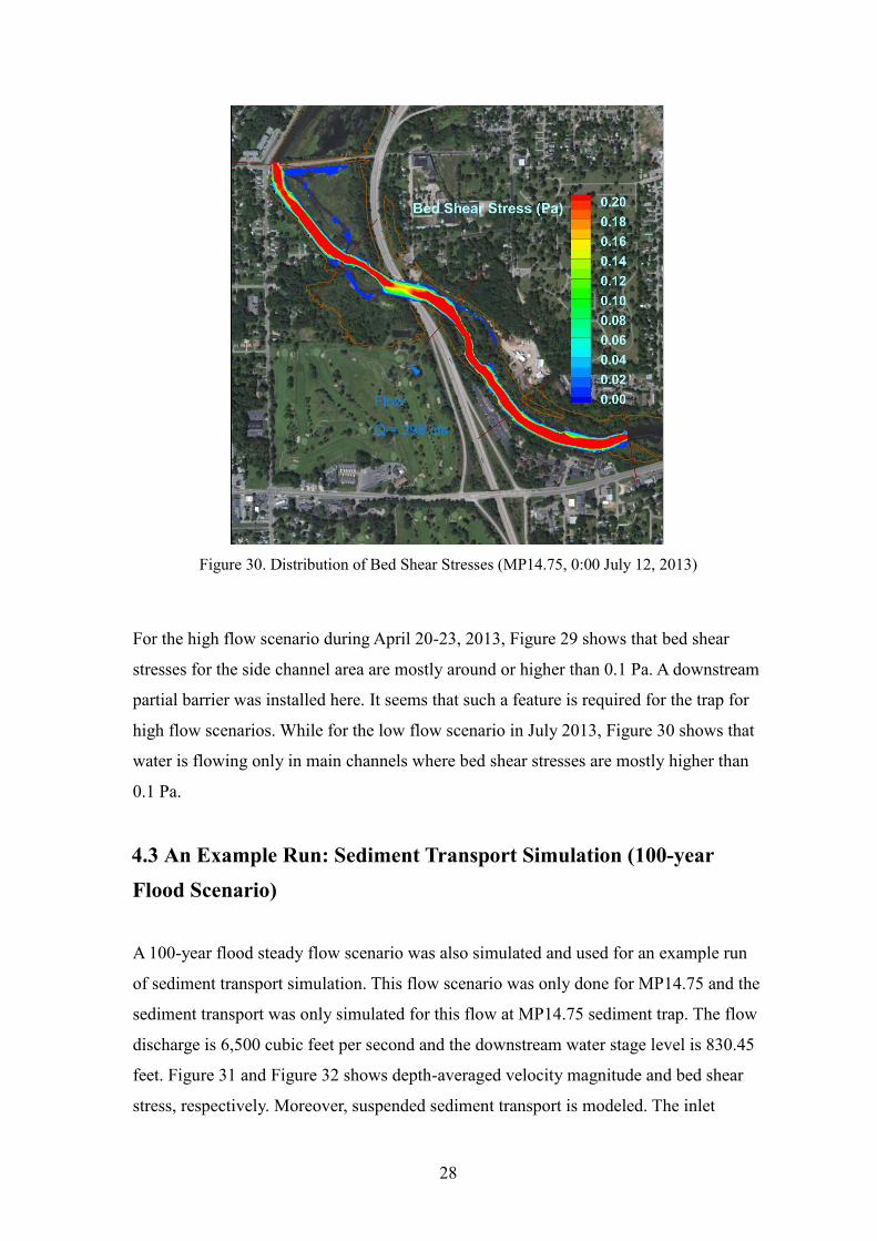
Figure 30. Distribution of Bed Shear Stresses (MP14.75, 0:00 July 12, 2013)
For the high flow scenario during April 20-23, 2013, Figure 29 shows that bed shear
stresses for the side channel area are mostly around or higher than 0.1 Pa. A downstream
partial barrier was installed here. It seems that such a feature is required for the trap for
high flow scenarios. While for the low flow scenario in July 2013, Figure 30 shows that
water is flowing only in main channels where bed shear stresses are mostly higher than
0.1 Pa.
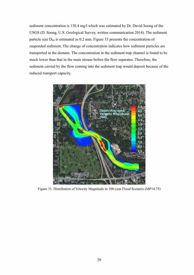
4.3 An Example Run: Sediment Transport Simulation (100-year Flood Scenario)
A 100-year flood steady flow scenario was also simulated and used for an example run
of sediment transport simulation. This flow scenario was only done for MP14.75 and the
sediment transport was only simulated for this flow at MP14.75 sediment trap. The flow
discharge is 6,500 cubic feet per second and the downstream water stage level is 830.45
feet. Figure 31 and Figure 32 shows depth-averaged velocity magnitude and bed shear
stress, respectively. Moreover, suspended sediment transport is modeled. The inlet
29
sediment concentration is 130.4 mg/l which was estimated by Dr. David Soong of the
USGS (D. Soong, U.S. Geological Survey, written communication 2014). The sediment
particle size D84 is estimated as 0.2 mm. Figure 33 presents the concentration of
suspended sediment. The change of concentration indicates how sediment particles are
transported in the domain. The concentration in the sediment trap channel is found to be
much lower than that in the main stream before the flow separates. Therefore, the
sediment carried by the flow coming into the sediment trap would deposit because of the
reduced transport capacity.
Figure 31. Distribution of Velocity Magnitude in 100-year Flood Scenario (MP14.75)

30
Figure 32. Distribution of Bed Shear Stresses in 100-year Flood Scenario (MP14.75)
Figure 33. Distribution of Suspended Sediment Concentration in 100-year Flood Scenario
(MP14.75)
31
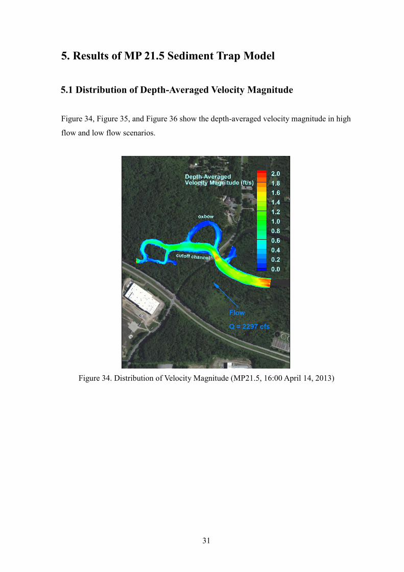
5. Results of MP 21.5 Sediment Trap Model
5.1 Distribution of Depth-Averaged Velocity Magnitude
Figure 34, Figure 35, and Figure 36 show the depth-averaged velocity magnitude in high
flow and low flow scenarios.
Figure 34. Distribution of Velocity Magnitude (MP21.5, 16:00 April 14, 2013)

32
Figure 35. Distribution of Velocity Magnitude (MP21.5, 16:00 April 21, 2013)
Figure 36. Distribution of Velocity Magnitude (MP21.5, 8:00 July 16, 2013)
33
The characteristic of this sediment trap is a cutoff channel. During the low flow period,
almost no water flows into the original meandering channel. However, during high
flows, some water with sediment may flow into the oxbow and sediment or OPAs would
deposit therein as Figure 40 indicates.
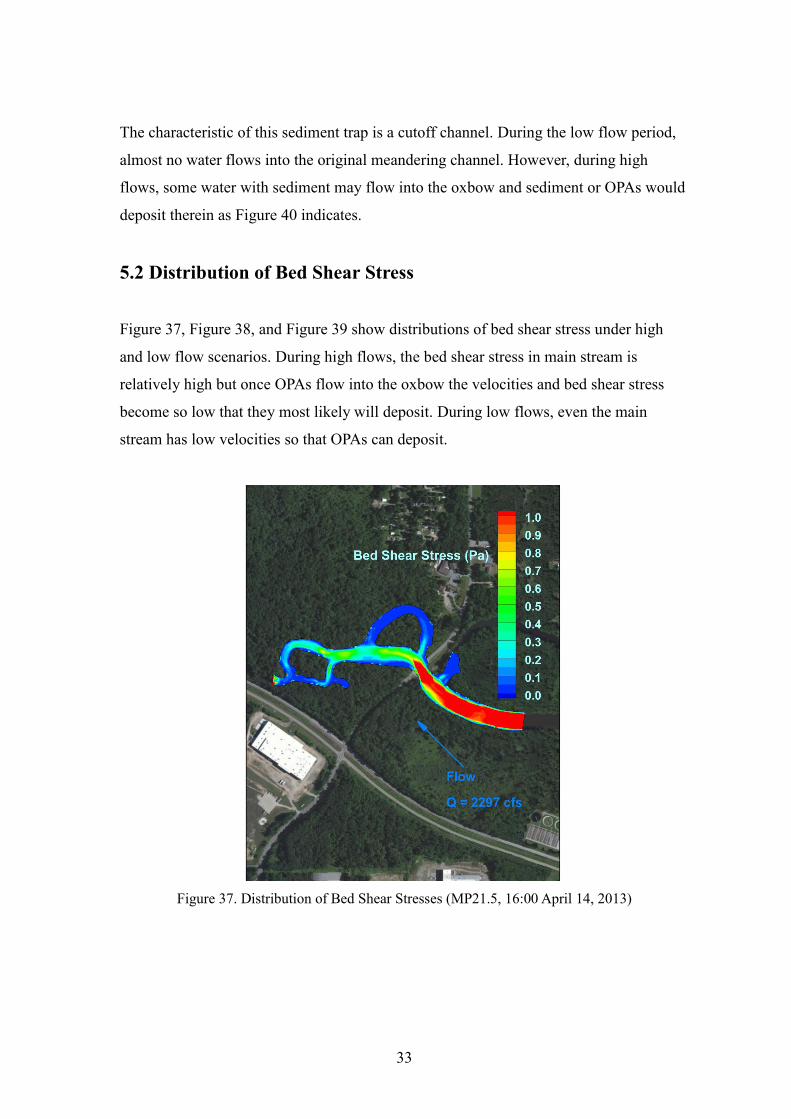
5.2 Distribution of Bed Shear Stress
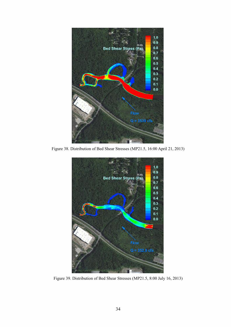
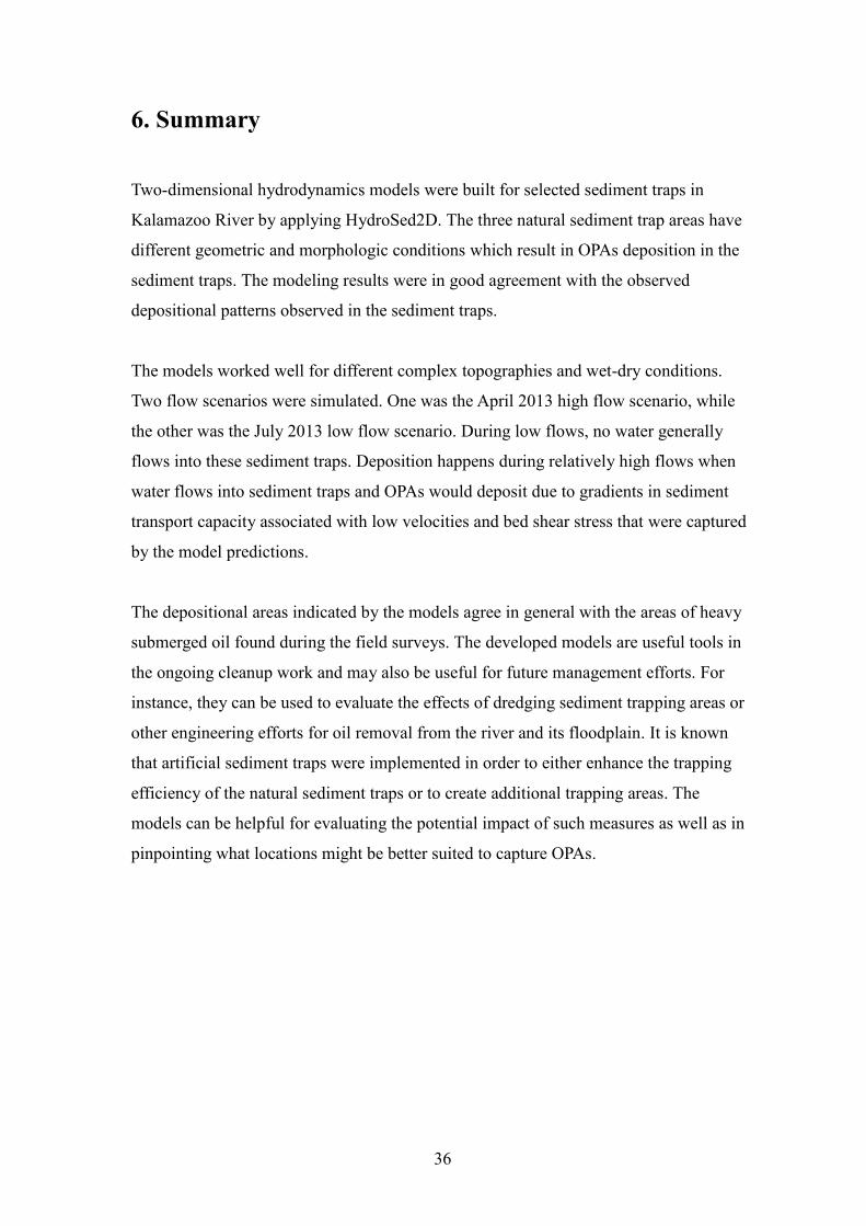
Figure 37, Figure 38, and Figure 39 show distributions of bed shear stress under high
and low flow scenarios. During high flows, the bed shear stress in main stream is
relatively high but once OPAs flow into the oxbow the velocities and bed shear stress
become so low that they most likely will deposit. During low flows, even the main
stream has low velocities so that OPAs can deposit.
Figure 37. Distribution of Bed Shear Stresses (MP21.5, 16:00 April 14, 2013)
34
Figure 38. Distribution of Bed Shear Stresses (MP21.5, 16:00 April 21, 2013)
Figure 39. Distribution of Bed Shear Stresses (MP21.5, 8:00 July 16, 2013)

35
Figure 40. Survey of Submerged Oil in the Modeling Domain of MP 21.5 (figure from the
Enbridge Energy, L.P. report [1])
36
6. Summary
Two-dimensional hydrodynamics models were built for selected sediment traps in
Kalamazoo River by applying HydroSed2D. The three natural sediment trap areas have
different geometric and morphologic conditions which result in OPAs deposition in the
sediment traps. The modeling results were in good agreement with the observed
depositional patterns observed in the sediment traps.
The models worked well for different complex topographies and wet-dry conditions.
Two flow scenarios were simulated. One was the April 2013 high flow scenario, while
the other was the July 2013 low flow scenario. During low flows, no water generally
flows into these sediment traps. Deposition happens during relatively high flows when
water flows into sediment traps and OPAs would deposit due to gradients in sediment
transport capacity associated with low velocities and bed shear stress that were captured
by the model predictions.
The depositional areas indicated by the models agree in general with the areas of heavy
submerged oil found during the field surveys. The developed models are useful tools in
the ongoing cleanup work and may also be useful for future management efforts. For
instance, they can be used to evaluate the effects of dredging sediment trapping areas or
other engineering efforts for oil removal from the river and its floodplain. It is known
that artificial sediment traps were implemented in order to either enhance the trapping
efficiency of the natural sediment traps or to create additional trapping areas. The
models can be helpful for evaluating the potential impact of such measures as well as in
pinpointing what locations might be better suited to capture OPAs.
37
Acknowledgments
The authors would like to thank Faith Fitzpatrick of the USGS Wisconsin Water Science
Center for coordination and help. David Soong of the USGS Illinois Water Science
Center is acknowledged for providing advice regarding the modeling and report. Rex
Johnson of GRT is acknowledged for providing data and other useful information.
Richard D. McCulloch of LimnoTech Inc. is acknowledged for providing the data which
was used as boundary conditions of the modeling efforts.
Special thanks are given to U.S. Environmental Protection Agency and Enbridge Energy,
L.P., contractors and collaborators involved in assessment and monitoring as well as
recovery and containment at the Kalamazoo River site.

38
Bibliography
1. Enbridge Energy, L.P., Sediment dredge depth and area determination addendum to
the 2013 submerged oil removal and assessment work plan (2013).
2. Goodwell, A. E. et al. Assessment of floodplain vulnerability during extreme
Mississippi river flood 2011. Environ. Sci. Technol. 48, 2619–25 (2014).
3. Liu, X., Landry, B. & Garcia, M. Two-dimensional scour simulations based on
coupled model of shallow water equations and sediment transport on unstructured
meshes. Coast. Eng. 55, 800–810 (2008).
4. Liu, X. et al. Sediment mobility and bed armoring in the St Clair River: insights from
hydrodynamic modeling. Earth Surf. Process. Landforms 37, 957–970 (2012).
5. Zhu, Z. Simulation of suspended sediment and contaminant transport in shallow
water using two-dimensional depth-averaged model with unstructured meshes.
Master Thesis, University of Illinois at Urbana-Champaign (2011).
6. Zhu, Z., Morales, V., Sinha, T. & García, M. Numerical modeling study on the
potential impacts of hydraulic structures in the Guayas watershed, Ecuador. The 7th
IAHR Symposium on River, Coastal and Estuarine Morphodynamics (RCEM) (2011).
7. LimnoTech. Kalamazoo River Hydrodynamic and Sediment Transport Model
Documentation (2014).
8. Weston. Bathymetry Report (2014).