PREDICTION OF FLOW IN NON PRISMATIC

COMPOUND OPEN CHANNEL USING ARTIFICIAL

NEURAL NETWORK

A Thesis Submitted in Partial Fulfillment of the Requirements for

the Degree of

Master of Technology

In

Civil Engineering

KAMEL MIRI

DEPARTMENT OF CIVIL ENGINEERING

NATIONAL INSTITUTE OF TECHNOLOGY,

ROURKELA 2013

Prediction of Flow in Non-prismatic Compound Open Channel

using Artificial Neural Network

A thesis

Submitted by

Kamil Miri

(212CE4516)

In partial fulfillment of the requirements

for the award of the degree of

Master of technology

In

Civil Engineering

(Water Resources Engineering)

Under The Guidance of

Dr. K. K. Khatu

Department of Civil Engineering

National Institute of Technology Rourkela

Orissa – 769008, India

May 2013

NATIONAL INSTITUTE OF TECHNOLOGY ROURKELA, ORISSA – 769008, INDIA

CERTIFICATE

This is to certify that the thesis entitled, “Prediction of Flow in Non prismatic

Compound Open Channel using Artificial Neural Network” submitted by Kamel Miri in

partial fulfillment of the requirement for the award of Master of Technology degree in

Civil Engineering with specialization in Water Resources Engineering at the

National Institute of Technology Rourkela is an authentic work carried out by him under our

supervision and guidance. To the best of our knowledge, the matter embodied in the thesis

has not been submitted to any other University/Institute for the award of any degree or

diploma.

Research Guide

Place: Rourkela

Date: 30/05/2014

Dr. K. K. Khatua Associate Professor

National Institute

Of Technology

ACKNOWLEDGEMENTS

First and foremost, praise and thanks goes to my God for the blessing that has bestowed upon

me in all my endeavors. I am deeply indebted to Dr. K.K Khatua, Associate Professor of

Water Resources Engineering Division, my advisor and guide, for the motivation, guidance,

tutelage and patience throughout the research work. I appreciate his broad range of expertise

and attention to detail, as well as the constant encouragement he has given me over the years.

There is no need to mention that a big part of this thesis is the result of joint work with him,

without which the completion of the work would have been impossible.

I am grateful to Prof. N Roy, Head of the Department of Civil Engineering for his

valuable suggestions and providing necessary facilities for the research work. And also i am

sincerely thankful to Prof. K.C. Patra, Prof. Ramakar Jha, and Prof. A. Kumar for their

kind cooperation and necessary advice. I extend my sincere thanks to Mrs. Bandita Naik

PhD. Scholar of Water Resources Engineering Division for their helpful comments and

encouragement for this work. I am grateful for friendly atmosphere of the Water

Resources Engineering Division and all kind and helpful professors that I have met during my

course.

I would like to thank my parents, Without their love, patience and support, I could not have

completed this work. Finally, I wish to thank many friends for the encouragement during these

difficult years.

KAMEL MIRI

I

ABSTRACT

Each river in the world is unique. Some are gently curved, others are meander, and some others are

relatively straight and skewed. The size of river geometry also changes from section to section

longitudinally due to different hydraulic and surface conditions called non-prismatic channel. Much

of the research work are found to be done on prismatic compound channels. There has also been a

progress of work found for meandering channels. But an era which has been neglected is that of the

work for non-prismatic compound channels. An effort has been made to scrutinize the research

work related to non-prismatic channels in different types of flow conditions. An experimental

observation has been made to investigate the velocity distribution, boundary shear stress distribution

and energy loss of a compound channel with converging flood plain. The calculation of Depth

average velocity, energy loss, boundary shear stress in non-prismatic compound channel flow is

more complex. The prediction of the flow characteristics in compound channels with prismatic and

non-prismatic floodplains is a challenging task for hydraulics engineers due to the three dimensional

nature of the flow. Simple conventional approaches cannot predict the above mentioned flow

characteristics with sufficient accuracy, hence in this area an easily implementable technique the

Artificial Neural Network can be used for prediction, validation and analysis of the flow parameters

mentioned. The model performed quite satisfactory when compared with the other conventional

methods.

II

TABLE OF CONTENTS

Title Page No.

CHAPTER 1 INTRODUCTION

1.1 OVERVIEW ...................................................................................................................................2

1.2 ARTIFICAL NEURAL NETWORK ............................................................................................4

1.2.1 Sigmoidal Function .....................................................................................................................6

1.2.2 Learning or training in back propagation neural networks .........................................................6

1.3 DEPTH AVERAGE VELOCITY DISTRIBUTION: ...................................................................7

1.3.1 Logarithmic law ..........................................................................................................................8

1.4 ENERGY AND ENERGY LOSS IN NON-PRISMATIC COMPOUND CHANNEL: ..............9

1.5 BOUNDARY SHEAR STRESS IN NON-PRISMATIC COMPOUND CHANNEL: ................9

1.6 OBJECTIVE OF PRESENT RESEARCH WORK: .................................................................. 11

1.7 ORGANIZATION OF THESIS: ................................................................................................ 13

CHAPTER 2 LITERATURE REVIEW

2.1 OVERVIEW ................................................................................................................................ 16

2.2 LITERATURE REVIEW RELATED TO THE RESEARCH WORK .................................... 17

PRESTON (1954) ............................................................................................................................. 17

BRADSHAW AND GREGORY (1959) AND HEAD AND RECHENBERG (1962) ................... 17

ZHELEZNYAKOV (1965) ............................................................................................................... 17

GHOSH AND JENA (1973) AND GHOSH AND MEHATA (1974) ............................................ 18

MYERS AND ELSWY (1975) ......................................................................................................... 18

MYERS (1978).................................................................................................................................. 18

RAJARATNAM AND AHMADI (1979) ........................................................................................ 18

RAJARATNAM AND AHMADI (1981) ........................................................................................ 18

WORMLEATON, ALEN, AND HADJIPANOS (1982) ................................................................. 19

KNIGHT AND DEMETRIOU (1983) ............................................................................................. 19

III

KNIGHT AND HAMED (1984) ...................................................................................................... 19

MCKEE ET AL. (1985) .................................................................................................................... 20

TOMINAGA ET AL. (1989) ............................................................................................................ 20

RHODES AND KNIGHT (1994) ..................................................................................................... 20

BOUSMAR (2002) AND BOUSMARET AL. (2004A) .................................................................. 20

(BOUSMAR ET AL., 2004B) .......................................................................................................... 20

PROUST (2005) AND PROUSTET AL.(2006) ............................................................................... 20

SARAT KUMAR DARS, PRABIR KUMAR BASUDHAR (2006) .............................................. 21

BOUSMARET AL. (2006) ............................................................................................................... 21

BAHRAM REZAEI (2006) .............................................................................................................. 21

SARAT KUMAR DAS, PRABIR KUMAR BASUDHAR (2008) ................................................. 21

A. BILGIL, H. ALTUN (2008) ......................................................................................................... 21

S.PROUST ET’AL (2008) ................................................................................................................ 22

PARAMESWAR PANDA (2010 ..................................................................................................... 22

REZAEI AND KNIGHT (2010) ....................................................................................................... 22

MRUTYUNJAYA SAHU, K.K.KHATUA, S.S.MAHAPATRA (2011) ........................................ 22

MRUTYUNJAYA SAHU (2011) ..................................................................................................... 22

MRUTYUNJAY SAHU, SRIJITA JANA, SONU AGARWAL, K.K. KHATUA (2011) ............. 22

REZAEI AND KNIGHT (2011) ....................................................................................................... 23

RAY SINGH MEENA (2012) .......................................................................................................... 23

MRUTYUNJAYA SAHU, PRASHANT SINGH, S.S.MAHAPATRA, K.K.KHATUA (2012) ... 23

CHAPTER 3 EXPERIMENTATION AND METHODOLOGY

3.1 OVERVIEW ................................................................................................................................ 25

3.2 DESIGN AND CONSTRUCTION OF CHANNEL .................................................................. 25

3.3 APPARATUS & EQUIPMENTS USED: .................................................................................. 28

3.4 EXPERIMENTAL PROCEDURE ............................................................................................. 30

3.4.1 MEASUREMENT OF DEPTH AVERAGE VELOCITY ..................................................... 32

IV

3.4.2 SOURCE OF DATA AND SELECTION OF HYDRAULIC PARAMETERS ................... 32

3.4.2.1 Selection Of Hydraulic, Geometric And Surface Parameters .............................................. 33

3.4.3 ANALYSIS OF ENERGY LOSSES AND INFLUENCING PARAMETERS ..................... 33

3.4.3.1 SELECTION OF HYDRAULIC PARAMETERS FOR ENERGY LOSS ......................... 35

3.4.4 SHEAR STRESS MEASUREMENTS ................................................................................... 35

3.4.4.1 Methods for estimation of Boundary shear stress ................................................................. 36

3.4.4.2 Selection of hydraulic parameters for Boundary Shear Stress ............................................. 37

3.4.5 MEASUREMENT OF BED SLOPE ....................................................................................... 38

CHAPTER 4 RESULTS

4.1 OVERVIEW ................................................................................................................................ 40

4.2 DEPTH AVERAGE VELOCITY RESULTS: ........................................................................... 41

4.3 ENERGY AND ENERGY LOSS RESULTS ............................................................................ 45

4.4 Boundary Shear Stress Distribution Results ............................................................................... 48

CHAPTER 5 CONCLUSION

SUMMARY: ..................................................................................................................................... 53

CONCLUSIONS: .............................................................................................................................. 54

REFERENCES .................................................................................................................................. 57

V

LIST OF FIGURES Figure 1.1 Typical stream wise velocity contour lines (isovels) for flow in various cross sections ...7

Figure 1.2 External Fluid flow across a flat plate ................................................................................8

Fig.1.3 3D flow structures in open channel ...................................................................................... 11

Fig.3.1 Plan view of compound channels with non-prismatic floodplains; (a) converging from 400

to 0mm along a 2m length (ONPC2-0); (b) narrowing from 400mm to 0 mm along a 6m length

(ONPC6-0) ........................................................................................................................................ 26

and; c)converging from 400mm to 200mm along a 6m length (ONPC6-200) ................................ 26

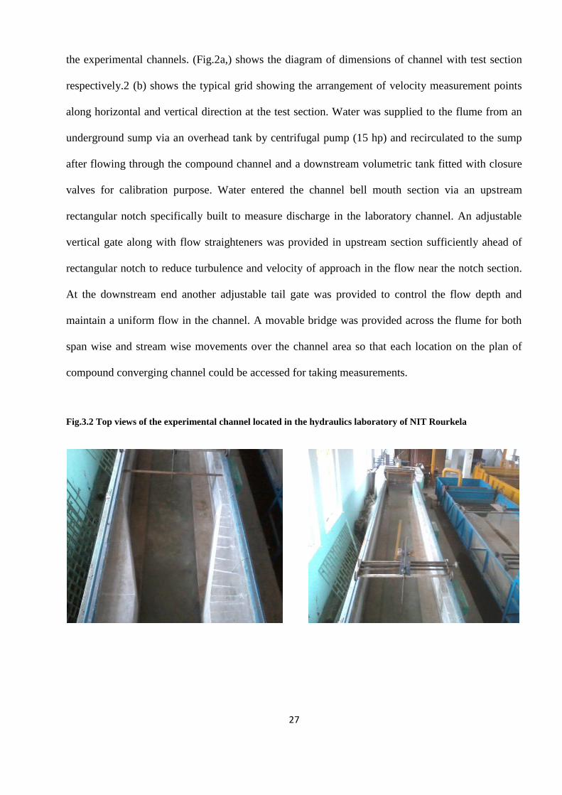
Fig.3.2 Top views of the experimental channel located in the hydraulics laboratory of NITR ....... 27

Fig.3.3 Series of Manometers ........................................................................................................... 28

Fig.3.4 Tail Gate ................................................................................................................................ 28

Fig.3.5 Non prismatic section of the channel ................................................................................... 29

Fig.3.6 Arrangements of the channel ................................................................................................ 29

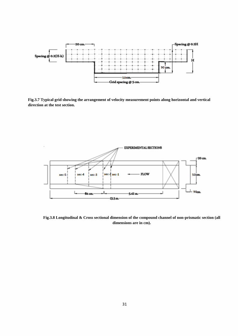
Fig.3.7 Typical grid showing the arrangement of velocity measurement points along horizontal and

vertical direction at the test section. .................................................................................................. 31

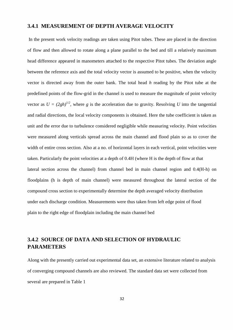
Fig.3.8 Longitudinal & Cross sectional dimension of the compound channel of non prismatic

section . .............................................................................................................................................. 31

Fig.3.9 Sketch of Energy profile of different section ....................................................................... 34

Fig.4.1 Details of the Neural Network tool in Matlab2010 .............................................................. 42

Fig.4.2 Correlation plot of actual depth average velocity and predicted depth average velocity .... 43

Fig.4.3 Comparison of actual and predicted depth average velocity (training data) ..................... 43

Fig.4.4 Comparison of actual and predicted depth average velocity ( testing data) ....................... 44

Fig. 4.5 Artificial Neural Network Structure .................................................................................... 45

Fig.4.6 Correlation plot of actual energy and predicted energy ....................................................... 46

Fig.4.7 Correlation plot of actual energy loss and predicted energy loss ......................................... 46

Fig.4.8 Residual distribution of training data of energy loss ............................................................ 47

Fig.4.9 Residual distribution of testing data of energy loss ............................................................. 48

VI

Fig.4.10 Correlation plot of actual boundary shear stress and predicted boundary shear stress

Residual analysis are carried out throughout the experimental studies and the results are presented

below ................................................................................................................................................. 49

Fig 4.11 Comparison of actual and predicted boundary shear stress (training data) ....................... 50

Fig.4.12 Comparison of actual and predicted boundary shear stress( testing data) ........................ 50

LIST OF TABLES Table 3.1 Hydraulic parameters for the experimental channel data set .......................................... 28

Table 4.1 Statistical Results of Emperical Equations in Calculations .............................................. 44

Table.4.2 Statistical results of empirical equation in Error Calculations of Energy Loss .............. 48

Table 4.3 Statistical Results of Empirical Equations in Error Calculations of Boundary Shear ..... 51

VII

LIST OF NOTATIONS

Wij Weight factor which represents interconnection of ith

node of the first

layer to the jth

node of the second layer

f Sigmoidal transfer function

Wkj Weight factor which represents interconnection of kth

node of the first

layer to the jth

node of the second layer

Ep Mean squared error for a pattern

W(t) Weight changes at any time t

n Learning rate

Momentum coefficient

𝛼 Width ratio

𝜎 Aspect ratio

𝜃 Angle of convergence of divergence

S Slope of the channel

B Channel cross section width

b Width of the main channel

h Main channel width

s Main channel side slopes

Dr Relative Depth

β Depth ratio

Xr The distance of the point velocity in the width wise of the cross

section / total width of the cross section taken into consideration.

Yr Distance of point velocity depth wise of the cross section / total depth

of the cross section taken into account.

Zr Point velocity in the length wise direction of the channel)/total length

of the non-prismatic channel.

z1 & z2 Bottom elevation above a given datum at section 1 and 2

respectively.

VIII

y1 & y2 the flow depths at section 1 and 2

v1 & v2 Mean velocities at section 1 and 2 respectively

h1 Local energy loss due to channel contraction

α1 & α2 Velocity head correction factors at section 1 and 2

E1 & E2 Energy at section 1 and section 2

P Pressure difference

o Boundary shear stress

d Outer diameter of the tube

ρ Density of the flow

ν Kinematic viscosity of the fluid

h Difference between the two readings of pitot tube, static and dynamic

heads

MSE Mean squared error

RMSE Root Mean squared error

MAE Mean absolute error

MAPE Mean absolute percentage error

ANN Artificial Neural Network

1

CHAPTER 1

INTRODUCTION

2

1.1 OVERVIEW

Water is perhaps the most fundamental and necessary resource available to mankind. It arrives

on land in the form of precipitation and returns to the sea by means of river channels. For the

most part, river channels adequately convey the water back to the sea but occasionally, under

conditions of high rainfall and large flow rates, the river channel may overtop its banks and flow

onto the flood plain with possible danger to life and property. Rivers are a natural aspect of

our landscape and form an integral part of the water cycle. By default rivers are the effect of

Magnificence and the historic essence of a settlement. Also rivers provide peace and

Serenity to human kind. People have lived near rivers for centuries due to the reason of mainly

food, water, transport and protection. But sometimes, it may cause serious damage to people

and the places in which they live even if it is a small, slow-flowing stream or gentle river.

Compound channels have been employed in river engineering for many years because of their

importance in environmental, ecological, and design issues related to flood defence schemes. One

advantage of two stage channels in the natural river, generally a main river channel and its

floodplain, is to increase the channel conveyance during floods. It is important to understand the

flow characteristics of rivers in both their inbank and overbank flow conditions. When the flow is

out-of-bank, typically during a flood, there is a significant increase in the complexity of flow

behavior, even for relatively straight reaches. The difference in velocity between the main channel

and the floodplain flows may produce strong lateral shear layers, which lead to the generation of

large scale turbulent structures, typically large platform vortices, as shown by Sellin (1964), Ikeda

et al. (1994 and 2001), Ikeda (1999) and Bousmar (2002). In overbank flow the main channel flow

is affected by the floodplains and the conveyance capacity is usually reduced. Open channel flow

can be said to be as the flow of fluid (water) over the deep hollow surface with the cover of

atmosphere at the top. Open channels are classified as the following.

1. Prismatic Open Channels

3

2. Non prismatic Open Channels

The open channel in which shape, size of cross section and slope of the bed remain constant are said

to be as the prismatic channels otherwise it is non prismatic channel. Natural channels are an

example of the non-prismatic channels and manmade open channels are the example of prismatic

channels. Some examples of non-prismatic channels are flow through culverts , flow through bridge

piers and obstructions, channel junction and etc. Study of non-prismatic river, distribution of flow

and velocity play a major role in relation to practical problems such as flood protection, flood plain

management, bank protection, navigation, water intakes and sediment transport-depositional

patterns.

The complexity of the problem rises more when dealing with a compound channel with non-

prismatic floodplains. In non prismatic compound channels with converging floodplains, due to

change in floodplain geometry water flowing on the floodplain now crosses over water flowing in

the main channel, resulting in increased interaction and momentum exchanges. This extra

momentum exchange should also be taken into account in the flow modelling. It is well known that

when the flow is out-of-bank the discharge capacity of a compound channel is affected by the

momentum exchange between the main channel and its associated floodplains. The momentum

transfer across the main channel/floodplain interface reduces the conveyance capacity of the main

channel and increases the discharge capacity of the floodplain, particularly at low relative depths,

and consequently reduces the total conveyance capacity of the entire channel cross section.

Experimental facilities, instrumentation and computer models have been gradually improved

in the world. In fact, for the last 2 or 3 decades, development of new velocity measuring devices,

data collection systems and numerical models has made possible considerable advances

in knowledge relating to water engineering problems.

4

The main objective of the depth average velocity measurements was to investigate the proportion of

flow in main channel and on the floodplains at different positions along the flume. The velocity

distributions were also used to investigate the force and energy balances in compound channels with

non-prismatic floodplains.

Using a pointer gauge, which was located on an instrument carriage, the longitudinal water profiles

have been recorded. The total energy head was estimated by adding the kinetic energy head to the

water surface profile level. The boundary shear stress distribution is another important parameter in

river modelling. It is required when studying force balances, or when calibrating a mathematical

model, which commonly requires knowledge of the variation of local resistance coefficients. To

evaluate the boundary shear stress distribution around the wetted perimeter, and the shear forces for

each relative depth, boundary shear stress measurements were performed at selected cross-sections.

1.2 ARTIFICAL NEURAL NETWORK

ANN is a new and rapidly growing computational technique. In recent years it has been broadly

used in hydraulic engineering and water resources. It is a highly self-organised, self-adapted and

self-trainable approximator with high associative memory and nonlinear mapping. ANNs can be

seen to be a simplified model of human nervous system, it can simulate complex and nonlinear

problems by employing a different number of nonlinear processing elements i.e. The nodes or

neurons. The nodes are connected by links or weights. ANNs may consists of multiple layers of

nodes interconnected with other nodes in the same or different layers. Various layers are referred to

as the input layer, the hidden layer and the output layer. The inputs and the inter connected weights

are processed by a weight summation function to produce a sum that is passed to a transfer function

The output of the transfer function is the output of the node.

In this research work multi-layer perception network is used. Input layer receives information from

the external source and passes this information to the network for processing. Hidden layer receives

5

information from the input layer and does all the information processing, and output layer receives

processed information from the network and sends the results out to an external receptor. The input

signals are modified by interconnection weight, known as weight factor wij which represents the

interconnection of ith node of the first layer to the jth node of the second layer. The sum of

modified signals (total activation) is then modified by a sigmoidal transfer function (f). Similarly

output signals of hidden layer are modified by interconnection weight (Wij) of kth node of output

layer to the jth node of the hidden layer. The sum modified k signal is then modified by a pure

linear transfer function (f) and output is collected at output layer.

Let Ip = (Ip1, Ip2,…,Ipl), p=1,2,…,N be the pth pattern among N input patterns.Wji and Wkj are

connection weights between ith input neuron to jth hidden neuron and jth hidden neuron to kth

output neuron respectively.

Output from a neuron in the input layer is

Opi=Ipi, i=1,2,…,l (1)

Output from a neuron in the hidden layer is

Opj = f (NETpj) = f(∑ ), j = 1,2,…,m (2)

Output from a neuron in the hidden layer is

Opk = f (NET pk) = f (∑ ), k=1,2,…,n (3)

6

1.2.1 Sigmoidal Function

A bounded, monotonic, non-decreasing, S Shaped function provides a graded nonlinear response. It

includes the logistic sigmoid function

F(x) =

(4)

Where x = input parameters taken

1.2.2 Learning or training in back propagation neural networks

Batch mode type of supervised learning has been used in the present case in which interconnection

weights are adjusted using delta rule algorithm after sending the entire training sample to the

network. During training the predicted output is compared with the desired output and the mean

square error is calculated.

If the mean square error is more, then a prescribed limiting value, It is back propagated from output

to input and weights are further modified till the error or number of iteration is within a prescribed

limit.

Mean Squared Error, Ep for pattern is defined as

Ep = ∑

( )

(5)

Where Dpi is the target output, Opi is the computed output for the ith pattern.

Weight changes at any time t, is given by

( ) ( ) 𝛼 ( ) (6)

n = learning rate i.e.

= momentum coefficient i.e.

7

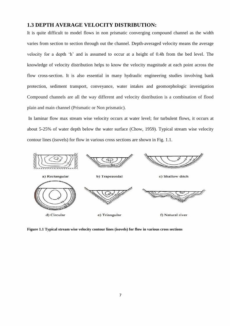
1.3 DEPTH AVERAGE VELOCITY DISTRIBUTION:

It is quite difficult to model flows in non prismatic converging compound channel as the width

varies from section to section through out the channel. Depth-averaged velocity means the average

velocity for a depth ‘h’ and is assumed to occur at a height of 0.4h from the bed level. The

knowledge of velocity distribution helps to know the velocity magnitude at each point across the

flow cross-section. It is also essential in many hydraulic engineering studies involving bank

protection, sediment transport, conveyance, water intakes and geomorphologic investigation

Compound channels are all the way different and velocity distribution is a combination of flood

plain and main channel (Prismatic or Non prismatic).

In laminar flow max stream wise velocity occurs at water level; for turbulent flows, it occurs at

about 5-25% of water depth below the water surface (Chow, 1959). Typical stream wise velocity

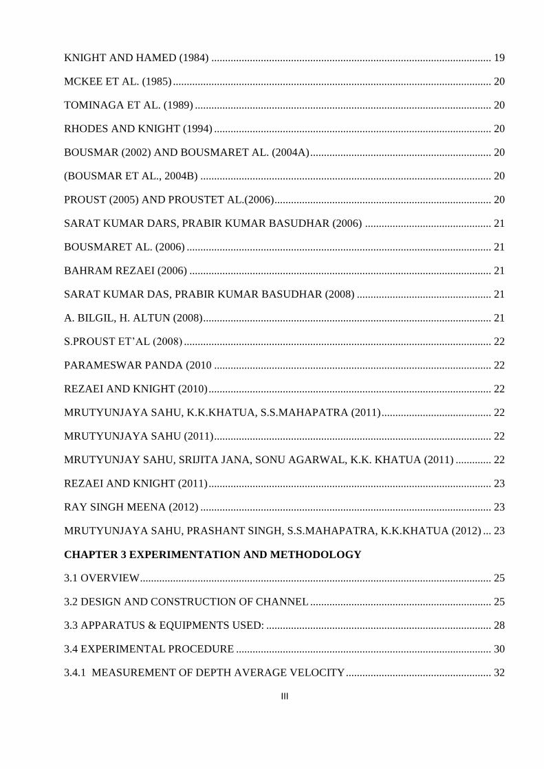
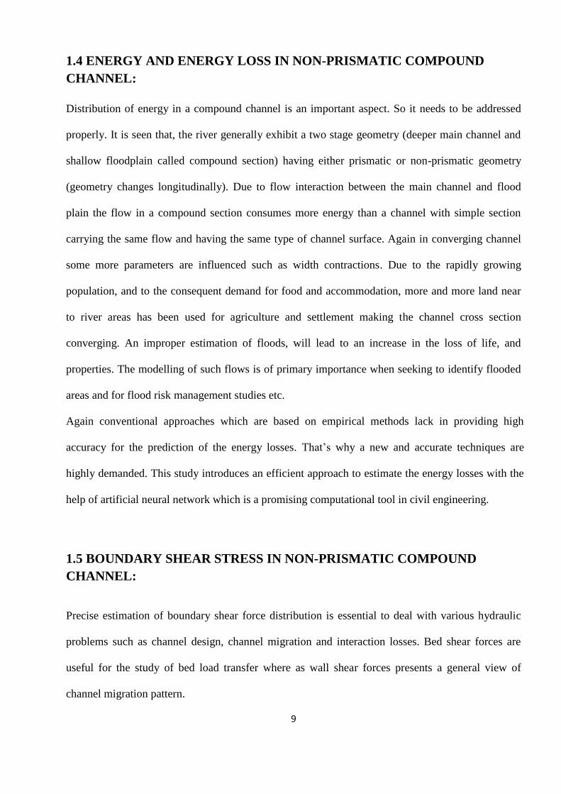
contour lines (isovels) for flow in various cross sections are shown in Fig. 1.1.

Figure 1.1 Typical stream wise velocity contour lines (isovels) for flow in various cross sections

8

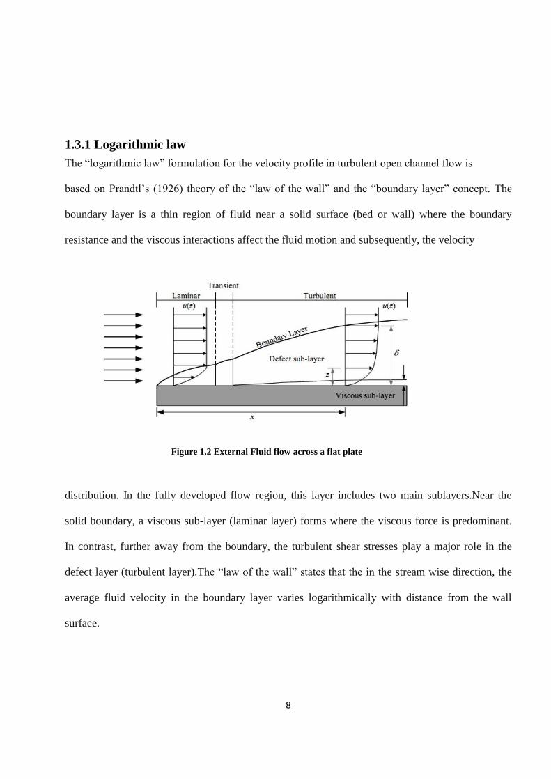
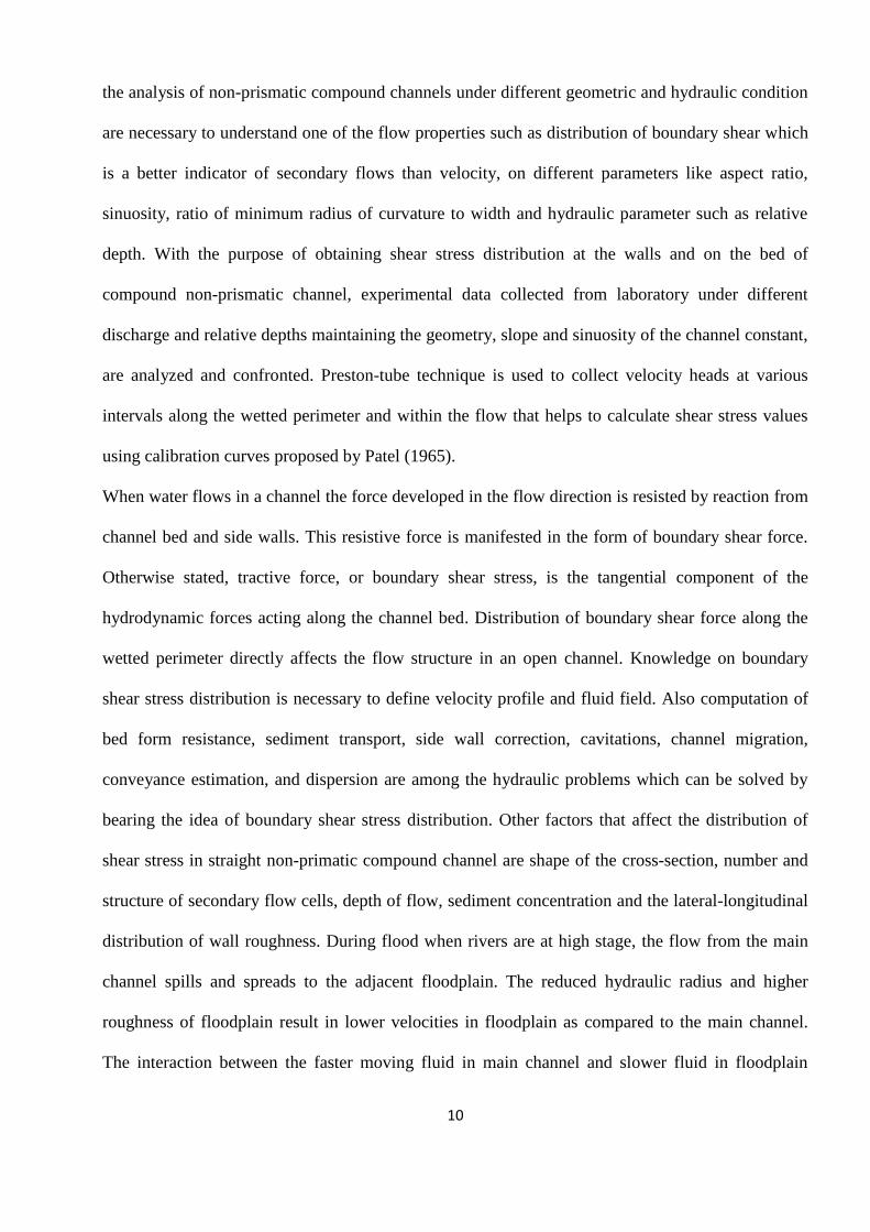
1.3.1 Logarithmic law

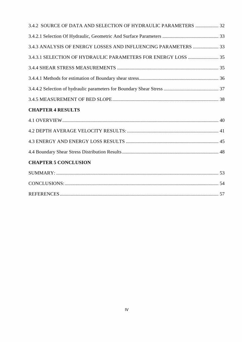
The “logarithmic law” formulation for the velocity profile in turbulent open channel flow is

based on Prandtl’s (1926) theory of the “law of the wall” and the “boundary layer” concept. The

boundary layer is a thin region of fluid near a solid surface (bed or wall) where the boundary

resistance and the viscous interactions affect the fluid motion and subsequently, the velocity

distribution. In the fully developed flow region, this layer includes two main sublayers.Near the

solid boundary, a viscous sub-layer (laminar layer) forms where the viscous force is predominant.

In contrast, further away from the boundary, the turbulent shear stresses play a major role in the

defect layer (turbulent layer).The “law of the wall” states that the in the stream wise direction, the

average fluid velocity in the boundary layer varies logarithmically with distance from the wall

surface.

Figure 1.2 External Fluid flow across a flat plate

9

1.4 ENERGY AND ENERGY LOSS IN NON-PRISMATIC COMPOUND

CHANNEL:

Distribution of energy in a compound channel is an important aspect. So it needs to be addressed

properly. It is seen that, the river generally exhibit a two stage geometry (deeper main channel and

shallow floodplain called compound section) having either prismatic or non-prismatic geometry

(geometry changes longitudinally). Due to flow interaction between the main channel and flood

plain the flow in a compound section consumes more energy than a channel with simple section

carrying the same flow and having the same type of channel surface. Again in converging channel

some more parameters are influenced such as width contractions. Due to the rapidly growing

population, and to the consequent demand for food and accommodation, more and more land near

to river areas has been used for agriculture and settlement making the channel cross section

converging. An improper estimation of floods, will lead to an increase in the loss of life, and

properties. The modelling of such flows is of primary importance when seeking to identify flooded

areas and for flood risk management studies etc.

Again conventional approaches which are based on empirical methods lack in providing high

accuracy for the prediction of the energy losses. That’s why a new and accurate techniques are

highly demanded. This study introduces an efficient approach to estimate the energy losses with the

help of artificial neural network which is a promising computational tool in civil engineering.

1.5 BOUNDARY SHEAR STRESS IN NON-PRISMATIC COMPOUND

CHANNEL:

Precise estimation of boundary shear force distribution is essential to deal with various hydraulic

problems such as channel design, channel migration and interaction losses. Bed shear forces are

useful for the study of bed load transfer where as wall shear forces presents a general view of

channel migration pattern.

10

the analysis of non-prismatic compound channels under different geometric and hydraulic condition

are necessary to understand one of the flow properties such as distribution of boundary shear which

is a better indicator of secondary flows than velocity, on different parameters like aspect ratio,

sinuosity, ratio of minimum radius of curvature to width and hydraulic parameter such as relative

depth. With the purpose of obtaining shear stress distribution at the walls and on the bed of

compound non-prismatic channel, experimental data collected from laboratory under different

discharge and relative depths maintaining the geometry, slope and sinuosity of the channel constant,

are analyzed and confronted. Preston-tube technique is used to collect velocity heads at various

intervals along the wetted perimeter and within the flow that helps to calculate shear stress values

using calibration curves proposed by Patel (1965).

When water flows in a channel the force developed in the flow direction is resisted by reaction from

channel bed and side walls. This resistive force is manifested in the form of boundary shear force.

Otherwise stated, tractive force, or boundary shear stress, is the tangential component of the

hydrodynamic forces acting along the channel bed. Distribution of boundary shear force along the

wetted perimeter directly affects the flow structure in an open channel. Knowledge on boundary

shear stress distribution is necessary to define velocity profile and fluid field. Also computation of

bed form resistance, sediment transport, side wall correction, cavitations, channel migration,

conveyance estimation, and dispersion are among the hydraulic problems which can be solved by

bearing the idea of boundary shear stress distribution. Other factors that affect the distribution of

shear stress in straight non-primatic compound channel are shape of the cross-section, number and

structure of secondary flow cells, depth of flow, sediment concentration and the lateral-longitudinal

distribution of wall roughness. During flood when rivers are at high stage, the flow from the main

channel spills and spreads to the adjacent floodplain. The reduced hydraulic radius and higher

roughness of floodplain result in lower velocities in floodplain as compared to the main channel.

The interaction between the faster moving fluid in main channel and slower fluid in floodplain

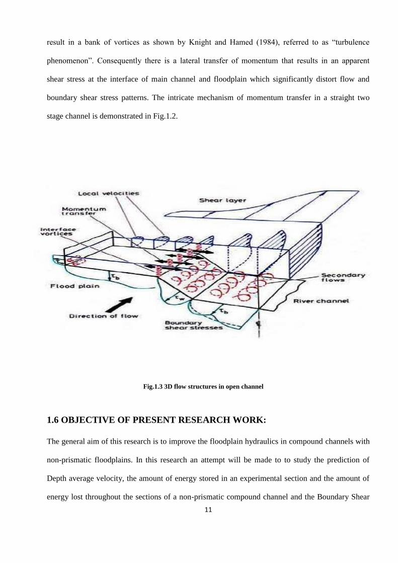
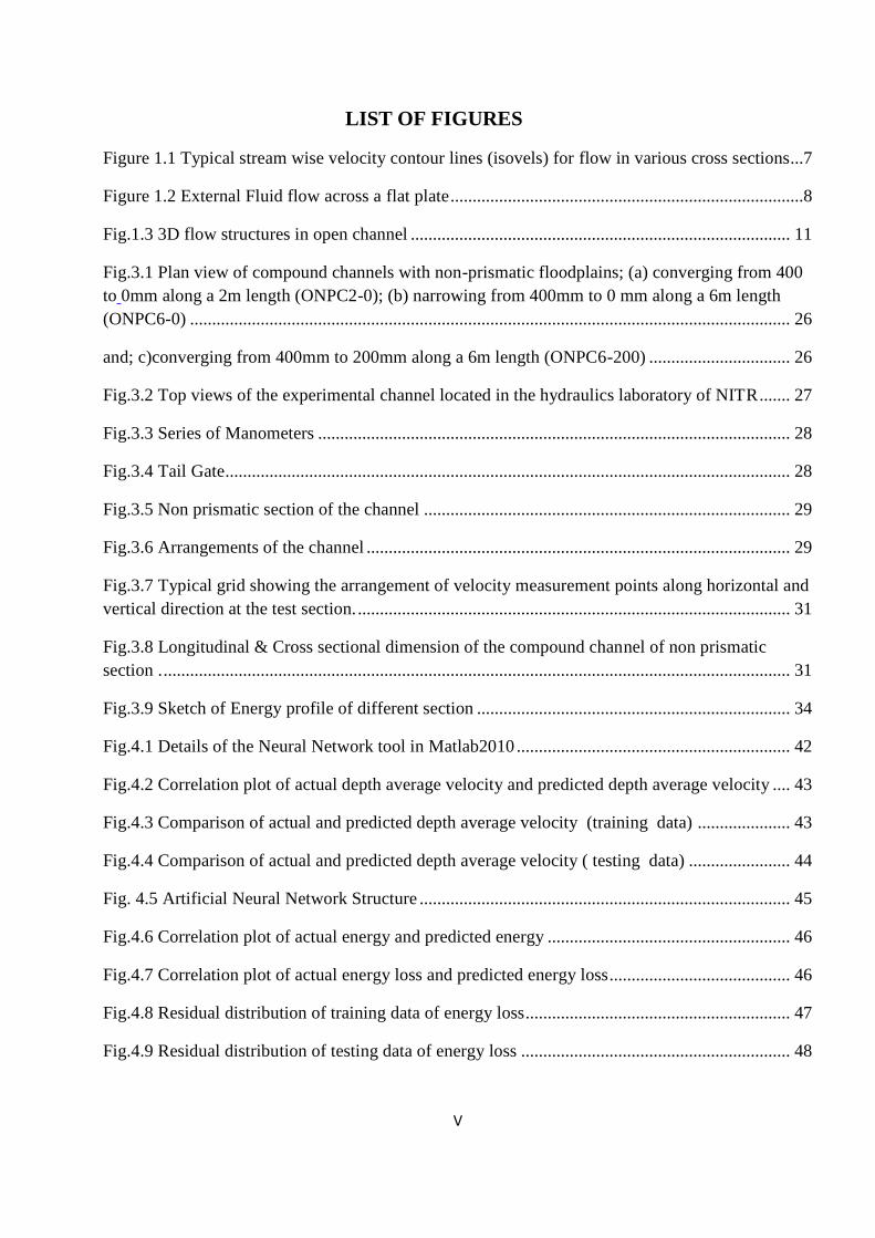
11

result in a bank of vortices as shown by Knight and Hamed (1984), referred to as “turbulence

phenomenon”. Consequently there is a lateral transfer of momentum that results in an apparent

shear stress at the interface of main channel and floodplain which significantly distort flow and

boundary shear stress patterns. The intricate mechanism of momentum transfer in a straight two

stage channel is demonstrated in Fig.1.2.

Fig.1.3 3D flow structures in open channel

1.6 OBJECTIVE OF PRESENT RESEARCH WORK:

The general aim of this research is to improve the floodplain hydraulics in compound channels with

non-prismatic floodplains. In this research an attempt will be made to to study the prediction of

Depth average velocity, the amount of energy stored in an experimental section and the amount of

energy lost throughout the sections of a non-prismatic compound channel and the Boundary Shear

12

stress generated throughout the sections of a non-prismatic compound channel using an Adaptive

Artificial Neural Network method.

Comparison will be made between the old conventional methods and the new and advised Adaptive

method of Artificial Neral Networks to see which method is more precise and accurate and gives

faster and brighter results.

The following specific aspects of river flood hydraulics will be investigated for non-prismatic

straight compound channels with overbank flow:

I. To study the distribution of stream wise depth-averaged velocity for a single flow depth,

also to study its variation at different flow depths for overbank flow conditions.

II. Determination of the amount of energy stored throughout the sections of a non-prismatic

compound channel and also the amount of energy lost throughout the experimental sections

of a non-prismatic compound channel.

III. To carry out an investigation concerning the distribution of local shear stress in the main

channel and flood plain of non-prismatic compound channel.

IV. Determination of boundary shear stress distribution along the wetted perimeter in non-

prismatic compound channels.

V. To conduct experiment and analyze experimental data for the investigation of longitudinal

wall and bed shear stress for different flow depths for compound non-prismatic open

channels.

13

VI. To devise an adaptive method specifically Artificial Nerual Network method to predict,

validate and compare the results of the study subjects with the old conventional methods.

VII. Comparison of the results obtained with the conventional techniques and analysis of the

precision and accuracy of the overall research work.

1.7 ORGANIZATION OF THESIS:

In this thesis an attempt has been made to predict flow parameters of a non-prismatic compound

channel using an adaptive system specifically the Artificial Neural Network. A prediction of Depth

average velocity, Energy stored and lost throughout the experimental channels and the Boundary

Shear Stress created throughout the experimental sections of the channel has been done using the

ANN technique. A comparison has been done between the actual results obtained and the predicted

results obtained and the accuracy of the ANN technique has been confirmed.

In this thesis the organization is as below

Chapter one is all about Introductions. First of all the Artificial Neural Network has been

introduced and the advances and the importance has been discussed. A slight understanding

on what actually the Depth average velocity, Energy loss and Boundary shear stress study

importance is and how they impact the phenomena. In this chapter the Objective of the

whole research study and the current thesis has also been mentioned.

Chapter two is all about the Literature review and the past studies that have been performed

on the Artificial Neural Networks. Studies conducted on non-prismatic compound channels

and the attempts to find out the velocity distributions, Energy and energy loss studies and

14

the Boundary shear stress studies have been discussed with the name of the researchers and

the year of study completion has been mentioned briefly and chronologically.

Chapter three discusses the Experimentation and Methodology of the current research work

with the detailed description of the experimentation process and the structure of the

experiment channel and all the apparatus and equipments used throughout the research

work. Measurements of the depth average velocity, the source of data selection, selection of

hydraulic geometry and surface parameters have been mentioned. The analysis of energy

loss and influencing parameters have been discussed and which factors are taken into

consideration in the selection of hydraulic parameters for the study are mentioned. The

measurements of Boundary shear stress have also been discussed in this chapter. The

measurement of the bed slope of the channel is also of the concerns in this chapter.

Chapter four is all about the Experimental Results that have been found after performing the

experimentations and analysis. All the graphs of the correlations and the residual analysis

are shown in the chapter in its respective study portions. The statistical results of the error

calculations are present to show the accuracy of the present research work

Chapter five an accumulation of the conclusions found from the results of the current

research work.

15

CHAPTER 2

LITERATURE REVIEW

16

2.1 OVERVIEW

An attempt has been made in this chapter to bring together various aspects of past research in

hydraulic engineering concerning the behavior of rivers and channels during overbank flow.

Until the early Sixties, little was known of the complex flow patterns which exist between a

channel and its flood plains, but recent developments have led to a clearer understanding of the

hydraulic mechanisms involved, at least at the level of model studies. An important step in

receiving a better understanding of river systems is to study its velocity distribution with

maximum accuracy. The flow prediction of river flows is vital information for flood control

channel design, channel stabilization and restoration projects and it affects the transport of

pollutants and sediments.

There are limited studies available in literature concerning the flow in non-prismatic compound

channel and the parameters affecting the flow specifically the Depth average velocity, the Energy

Loss throughout the channel and the Boundary shear stress developed.

Studies are required to be conducted on these aspects as these are the heart and soul of the water

characteristics in a non-prismatic compound channel and are very much essential for water

engineers.

The literature review contains a large body of research on the subjects of Depth average velocity,

Energy and Energy Loss, Boundary Shear stress and mainly on the previous research works that

have used Artificial neural network as their primary and adaptive method for analysis and

predictions carried out in open channel flows. This review intends to present some of the selected

significant contribution to the study of the mentioned aspects from earlier times to the most recent

ones available.

17

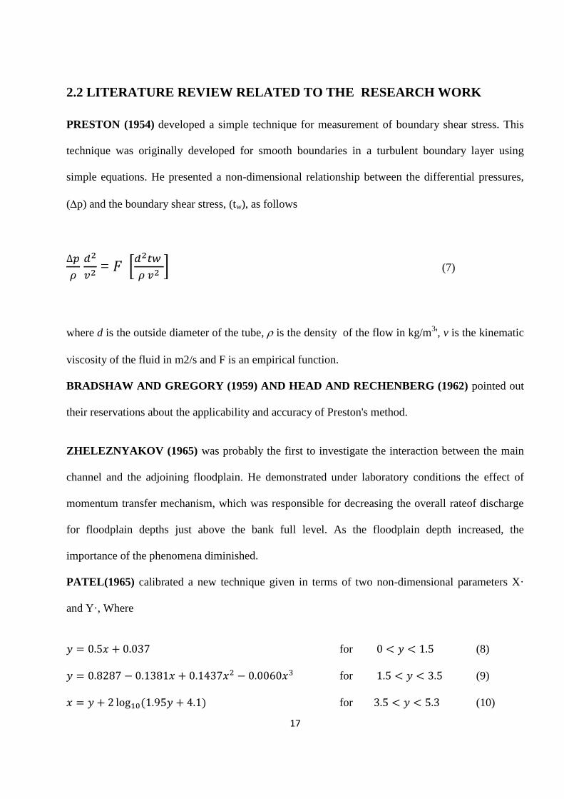
2.2 LITERATURE REVIEW RELATED TO THE RESEARCH WORK

PRESTON (1954) developed a simple technique for measurement of boundary shear stress. This

technique was originally developed for smooth boundaries in a turbulent boundary layer using

simple equations. He presented a non-dimensional relationship between the differential pressures,

(p) and the boundary shear stress, (tw), as follows

= [

] (7)

where d is the outside diameter of the tube, is the density of the flow in kg/m3', v is the kinematic

viscosity of the fluid in m2/s and F is an empirical function.

BRADSHAW AND GREGORY (1959) AND HEAD AND RECHENBERG (1962) pointed out

their reservations about the applicability and accuracy of Preston's method.

ZHELEZNYAKOV (1965) was probably the first to investigate the interaction between the main

channel and the adjoining floodplain. He demonstrated under laboratory conditions the effect of

momentum transfer mechanism, which was responsible for decreasing the overall rateof discharge

for floodplain depths just above the bank full level. As the floodplain depth increased, the

importance of the phenomena diminished.

PATEL(1965) calibrated a new technique given in terms of two non-dimensional parameters X·

and Y·, Where

for (8)

for (9)

( ) for (10)

18

Following Patel's calibration, many investigators have studied boundary shear stress distributions in

different channel geometries using the Preston tube.

GHOSH AND JENA (1973) AND GHOSH AND MEHATA (1974) reported studies on boundary

shear distribution in straight two stage channels for both smooth and rough boundaries. They found

the distribution of shear is non-uniform and the location of maximum bed and side shear to be some

distance from the centreline and free surface. They related the sharing of the total drag force by

different segments of the channel section to the depth of flow and roughness concentration.

MYERS AND ELSWY (1975) studied the effect of interaction mechanism and shear stress

distribution in channels of complex sections. In comparison to the values under isolated condition,

the results showed a decrease up to 22 percent in channel shear and increase up to 260 percent in

floodplain shear. This indicated the possible regions of erosion and scour of the channel and flow

distribution in alluvial compound sections.

MYERS (1978) studied the momentum transfer mechanism and found the apparent shear stresses

were significantly greater than those exerted on a solid boundary or floodplain wall at the interface.

RAJARATNAM AND AHMADI (1979) studied the flow interaction between straight main

channel and symmetrical floodplain with smooth boundaries. The results demonstrated the transport

of longitudinal momentum from main channel to flood plain. Due to flow interaction, the bed shear

in floodplain near the junction with main channel increased considerably and that in the main

channel decreased. The effect of interaction reduced as the flow depth in the floodplain increased.

RAJARATNAM AND AHMADI (1981) showed that the boundary shear stress reduces from the

centre of the main channel toward the edge of the floodplain and then sharply increases at the

19

interface between the main channel and the floodplain. They also stated that, due to interaction

between subsections in compound channels, the boundary shear stress in the main channel reduces

WORMLEATON, ALEN, AND HADJIPANOS (1982) undertook a series of laboratory tests in

straight channels with symmetrical floodplains and used "divide channel" method for the

assessment of discharge. From the measurement of boundary shear, apparent shear stress at the

vertical, horizontal, and diagonal interface plains originating from the main channel floodplain

junction could be evaluated. An apparent shear stress ratio was proposed which was found to be a

useful yardstick in selecting the best method of dividing the channel for calculating discharge. It

was found that under general circumstances, the horizontal and diagonal interface method of

channel separation gave better discharge results than the vertical interface plain of division at low

depths of flow in the floodplains.

KNIGHT AND DEMETRIOU (1983) conducted experiments in straight symmetrical compound

channels to understand the discharge characteristics, boundary shear stress and boundary shear force

distributions in the section. They presented equations for calculating the percentage of shear force

carried by floodplain and also the proportions of total flow in various sub-areas of compound

section in terms of two dimensionless channel parameters. For vertical interface between main

channel and floodplain the apparent shear force was found to be more at low depths of flow and

also for high floodplain widths. On account of interaction of flow between floodplain and main

channel, it was found that the division of flow between the sub-areas of the compound channel did

not follow the simple linear proportion to their respective areas.

KNIGHT AND HAMED (1984) extended the work of Knight and Demetriou (1983) to rough

floodplains. The floodplains were roughened progressively in six steps to study the influence of

20

different roughness between floodplain and main channel to the process of lateral momentum

transfer. Using four dimensionless channel parameters, they presented equations for the shear force

percentages carried by floodplains and the apparent shear force in vertical, horizontal, diagonal, and

bisector interface plains. The apparent shear force results and discharge data provided the strength

and weakness of these four commonly adopted design methods used to predict the discharge

capacity of the compound channel.

MCKEE ET AL. (1985) confirmed Myers momentum balance approach using the Laser Doppler

Anemometry (LDA) technique.

TOMINAGA ET AL. (1989) the boundary shear stress is highly affected by the secondary flow,

and it increases where the secondary currents flow toward the wall and decreases when they flow

away from the wall.

RHODES AND KNIGHT (1994) suggested that the bank slope had a significant effect on the

boundary shear stress distributions at the interface between the main channel and floodplain.

BOUSMAR (2002) AND BOUSMARET AL. (2004A) Analysed the experiments on converging

compound channels with symmetrically narrowing floodplains. They highlighted the geometrical

momentum transfer and the associated additional head loss due to symmetrically narrowing

floodplains force flow from the floodplains to the main channel. They estimated the additional head

loss due to the mass transfer. Its value was found in several cases as large as the friction loss.

(BOUSMAR ET AL., 2004B) Performed additional investigations using digital imaging to record

surface velocities and horizontal turbulent structures that generally develop in prismatic channels.

PROUST (2005) AND PROUSTET AL.(2006) Investigated the flow analysis of a compound

channel with asymmetric geometry with a more abrupt convergence. They found that a larger mass

21

transfer and total head loss is resulting from the higher convergence angle. The total head within the

main channel decreased faster than that in flood plain.

SARAT KUMAR DARS, PRABIR KUMAR BASUDHAR (2006) The paper described the

application of the artificial neural network model to predict the lateral load capacity of piles in clay.

Three criteria were selected to compare the ANN model with the available empirical models. model

equation is presented based on neural network parameters.

BOUSMARET AL. (2006) Investigated diverging compound channels, with symmetrically

enlarging floodplains. He found the water profile rise in downstream direction. Due to deceleration

the mean velocity decreased in downstream direction. Head losses increased in non prismatic

section.

BAHRAM REZAEI (2006) Presented the experimental results of non-prismatic compound

channels with converging floodplains, due to change in floodplain geometry. They found that, water

flowing on the floodplain is crossing over water flowing in the main channel, resulting in increased

interactions and momentum exchanges.

SARAT KUMAR DAS, PRABIR KUMAR BASUDHAR (2008) This paper presents a neural

network model to predict the residual friction angle based on clay fraction and Atterberg's limits.

Emphasis is placed on theconstruction of neural interpretation diagram, based on the weights of the

developed neural network model, to find out direct or inverse effect of soil properties on the

residual shear angle. A prediction model equation is established with the weights of the neural

network as the model parameters.

A. BILGIL, H. ALTUN (2008) Investigated the flow resistance in smooth open channels using

Artificial Neural Networks. The estimated values of friction coefficient is used in Manning’s

Equation to predict the open channel flows in order to carry out a comparison between the

proposed neural networks based approach and the conventional ones.

22

S.PROUST ET’AL (2008) Evaluated the relative weights of three sources of energy loss for non-

uniform flows in compound channel: (1) the bed friction; (2) the momentum transfer due to

turbulent exchange between the main channel and the floodplains; and (3) the momentum transfer

due to mass exchange between the subsections. They also found that in compound channels with

non-prismatic floodplains, the apparent shear forces in vertical interface are negative.

PARAMESWAR PANDA (2010) Predicted the flow in compound open channel using Artificial

Neural Network. An ANN Algorithm has been developed to predict discharge capacity of

compound channels observed at 190 comprehensive laboratory data of various experiments across

the ingenious laboratory experiments done in NIT Rourkela.

REZAEI AND KNIGHT (2010) gave a modified SKM method to investigate the various

converging angles and relative depths.

MRUTYUNJAYA SAHU, K.K.KHATUA, S.S.MAHAPATRA (2011) used a neural network

approach for prediction of discharge in straight compound open channel flow. Discharge

determination models such as the single channel method (SCM), the divided channel method

(DCM), the coherence method (COHM) and the exchange discharge method (EDM) are widely

used; however they are insufficient to predict discharge accurately therefor and attempt has been

made to predict the total discharge in compound open channels with and Artificial neural network

and compare it with the above models.

MRUTYUNJAYA SAHU (2011) predicted the flow and its resistance in compound open channel

using adaptive approaches such as Artificial neural networks and adaptive fuzzy interference system

for different hydraulic conditions.

MRUTYUNJAY SAHU, SRIJITA JANA, SONU AGARWAL, K.K. KHATUA (2011) point

form velocity in the downstream of flow is predicted at different sections of the meandering

23

channel. Back propagation learning rule in ANN network is considered for further analysis, as this

network is well adept with pattern recognition and forecasting. In this further analysis, position of

the point and depth of flow are taken as input and point form velocity is the output.

REZAEI AND KNIGHT (2011) found that for the lower water depths, the discharge evolution

seems linear; whereas for higher water depths, it is nonlinear. The mass transfer in the second half

of the converging reach is higher than that in the first half. They further found that in compound

channels with non-prismatic floodplains, the apparent shear forces in vertical interface are negative.

RAY SINGH MEENA (2012) introduced about the parameterization of hydrologic and hydraulic

modeling for simulation of runoff and flood inundated area mapping. Results indicated that for Kosi

catchment, the empirical runoff prediction approach (ANN technique), in spite of requiring much

less data, predicted daily runoff values more accurately than semi-distributed conceptual runoff

prediction approach (SCS-CN method).

MRUTYUNJAYA SAHU, PRASHANT SINGH, S.S.MAHAPATRA, K.K.KHATUA (2012)

proposed an adaptive network fuzzy interference system for the prediction of entrance length in pipe

for low Reynolds number flow.

24

CHAPTER 3

EXPERIMENTATION AND

METHODOLOGY

25

3.1 OVERVIEW

Normally experimental work should be conducted on natural streams for non-prismatic compound

channels, but because of the time consuming process and the fact that natural streams are difficult to

have access to in our recent locational condition, we have restrained our work to only laboratory work

and laboratory modeling for the non-prismatic compound channel in which we have performed our

experiments and have recorded the readings for the analysis of different flow parameters, so all our

research work has been restricted to laboratory modeling and the artificial channel built inside the

laboratory indicating the real aspect of non-prismatic compound channels.

Experiments have been conducted on the non-prismatic compound channel located in the Hydraulics

laboratory of National Institute of Rourkela for analysis and study of different parameters influencing

flow in non-prismatic compound channel specifically Depth average velocity, Energy stored and

Energy lost throughout the experimental sections of the channel and finally the Boundary Shear Stress

developed in each experimental section of the channel taken into consideration.

Besides the fact that National Institute of Technology Rourkela had limited resources and limited

experimental facilities, still the study was carried out quite satisfactory and was completed with the

guidance of experienced and hardworking professors of water resources specifically Dr. K. K. Khatua

and other hardworking staff of Water Resources specialization

3.2 DESIGN AND CONSTRUCTION OF CHANNEL

Experiments have been conducted in two sets of non-prismatic compound channels with varying

cross section built inside a concrete flume measuring 15m long ×.90m width × 0.55m depth and

flume with perpexsheet of same dimensions. The width ratio of the channel is α=1.8 and the aspect

ratio is σ=5 where width ratio is the ratio between width of floodplain to width of main channel and

aspect ratio is the ratio between width of channel to depth of flow. The converging angle of the

channels are taken as 12.38° and 50

( Naik 2014 ).Converging length of the channel is found to be

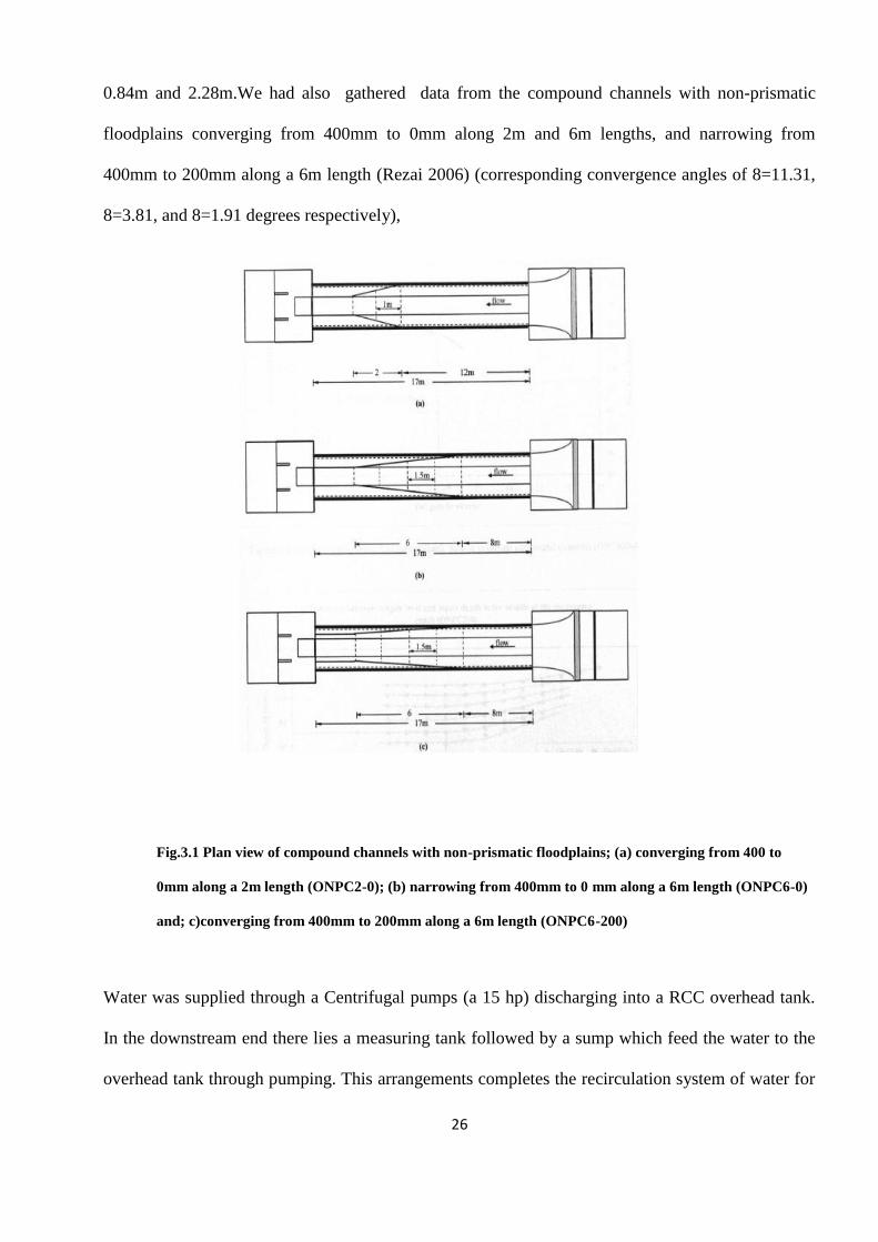
26

0.84m and 2.28m.We had also gathered data from the compound channels with non-prismatic

floodplains converging from 400mm to 0mm along 2m and 6m lengths, and narrowing from

400mm to 200mm along a 6m length (Rezai 2006) (corresponding convergence angles of 8=11.31,

8=3.81, and 8=1.91 degrees respectively),

Fig.3.1 Plan view of compound channels with non-prismatic floodplains; (a) converging from 400 to

0mm along a 2m length (ONPC2-0); (b) narrowing from 400mm to 0 mm along a 6m length (ONPC6-0)

and; c)converging from 400mm to 200mm along a 6m length (ONPC6-200)

Water was supplied through a Centrifugal pumps (a 15 hp) discharging into a RCC overhead tank.

In the downstream end there lies a measuring tank followed by a sump which feed the water to the

overhead tank through pumping. This arrangements completes the recirculation system of water for

27

the experimental channels. (Fig.2a,) shows the diagram of dimensions of channel with test section

respectively.2 (b) shows the typical grid showing the arrangement of velocity measurement points

along horizontal and vertical direction at the test section. Water was supplied to the flume from an

underground sump via an overhead tank by centrifugal pump (15 hp) and recirculated to the sump

after flowing through the compound channel and a downstream volumetric tank fitted with closure

valves for calibration purpose. Water entered the channel bell mouth section via an upstream

rectangular notch specifically built to measure discharge in the laboratory channel. An adjustable

vertical gate along with flow straighteners was provided in upstream section sufficiently ahead of

rectangular notch to reduce turbulence and velocity of approach in the flow near the notch section.

At the downstream end another adjustable tail gate was provided to control the flow depth and

maintain a uniform flow in the channel. A movable bridge was provided across the flume for both

span wise and stream wise movements over the channel area so that each location on the plan of

compound converging channel could be accessed for taking measurements.

Fig.3.2 Top views of the experimental channel located in the hydraulics laboratory of NIT Rourkela

28

Table 3.1 Hydraulic parameters for the experimental channel data set collected from literature & experiments

Verified test channel

Types of channel

Angle of convergent/Diver

gent

Longitud

inal

slope

(S)

Cross sectional geometry

Total channel width (B) in

m

Main channel

width (b) in m

Main channel

depth (h) in m

Main channel side

slope ( s )

Width ratio B/b

()

1 2 3 4 5 7 8 9 10 11

Rezai(2006) Convergent

(CV2) (Ɵ=11.31°,2m ) 0.002 Rectangular 1.2 0.398 0.05 0 3

Rezai(2006)) Convergent

(CV6) (Ɵ=3.81°,6m ) 0.002 Rectangular 1.2 0.398 0.05 0 3

Rezai(2006) Convergent

(CV6) (Ɵ=1.91°,6m) 0.002 Rectangular 1.2 0.398 0.05 0 3

N.I.T.Rkl data Convergent (Ɵ=5°,2.28m) 0.0011 Rectangular 0.9 0.5 0.1 0 1.8

N.I.T.Rkl data Convergent

(Ɵ=12.38°,0.84m 0.0017 Rectangular 0.9 0.5 0.1 0 1.8

3.3 APPARATUS & EQUIPMENTS USED:

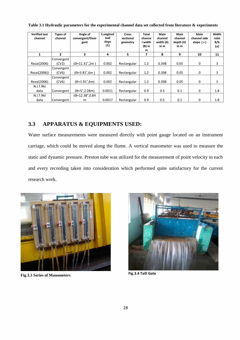
Water surface measurements were measured directly with point gauge located on an instrument

carriage, which could be moved along the flume. A vertical manometer was used to measure the

static and dynamic pressure. Preston tube was utilized for the measurement of point velocity in each

and every recording taken into consideration which performed quite satisfactory for the current

research work.

Fig.3.4 Taill Gate Fig.3.3 Series of Manometers

29

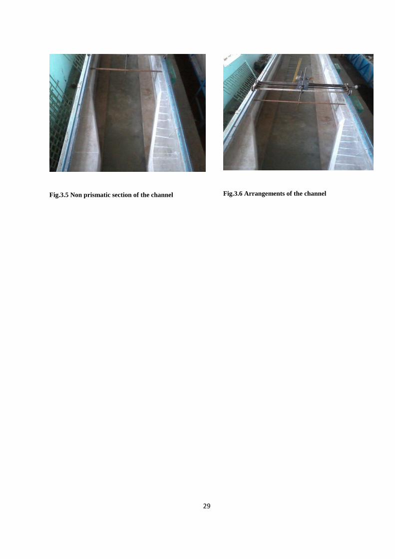
Fig.3.6 Arrangements of the channel Fig.3.5 Non prismatic section of the channel

30

3.4 EXPERIMENTAL PROCEDURE

The measurements were made each 5mm and 10mm in converging flume of .840 m and 2.28m

length. Point velocities were measured along verticals spread across the main channel and flood

plain so as to cover the width of entire cross section. Also at a no. of horizontal layers in each

vertical, point velocities were measured. Measurements were thus taken from mid-point of main

channel to the left edge of floodplain. The lateral spacing of grid points over which measurements

were taken was kept 5cm inside the main channel and the flood plain. Velocity measurements were

taken by Pitot static tube (outside diameter 4.77mm) and two piezometers fitted inside a transparent

fibre block fixed to a wooden board and hung vertically at the edge of flume the ends of which were

open to atmosphere at one end and connected to total pressure hole and static hole of Pitot tube by

long transparent PVC tubes at other ends. Before taking the readings the Pitot tube along with the

long tubes measuring about 5m were to be properly immersed in water and caution was exercised

for complete expulsion of any air bubble present inside the Pitot tube or the PVC tube. Even the

presence of a small air bubble inside the static limb or total pressure limb could give erroneous

readings in piezometers used for recording the pressure. The angle of limb of Pitot tube with

longitudinal direction of the channel was noted by circular scale and pointer arrangement attached

to the flow direction meter. Pitot tube was physically rotated with respect to the main stream

direction till it recorded the maximum deflection of the manometer reading. A flow direction finder

was used to get the direction of maximum velocity with respect to the longitudinal flow direction.

Steady uniform discharge was maintained the run of the experiment and several runs were

conducted for overbank flow with relative depth varying between 0.15-0.51.

31

Fig.3.7 Typical grid showing the arrangement of velocity measurement points along horizontal and vertical

direction at the test section.

Fig.3.8 Longitudinal & Cross sectional dimension of the compound channel of non-prismatic section (all

dimensions are in cm).

32

3.4.1 MEASUREMENT OF DEPTH AVERAGE VELOCITY

In the present work velocity readings are taken using Pitot tubes. These are placed in the direction

of flow and then allowed to rotate along a plane parallel to the bed and till a relatively maximum

head difference appeared in manometers attached to the respective Pitot tubes. The deviation angle

between the reference axis and the total velocity vector is assumed to be positive, when the velocity

vector is directed away from the outer bank. The total head h reading by the Pitot tube at the

predefined points of the flow-grid in the channel is used to measure the magnitude of point velocity

vector as U = (2gh)1/2

, where g is the acceleration due to gravity. Resolving U into the tangential

and radial directions, the local velocity components is obtained. Here the tube coefficient is taken as

unit and the error due to turbulence considered negligible while measuring velocity. Point velocities

were measured along verticals spread across the main channel and flood plain so as to cover the

width of entire cross section. Also at a no. of horizontal layers in each vertical, point velocities were

taken. Particularly the point velocities at a depth of 0.4H (where H is the depth of flow at that

lateral section across the channel) from channel bed in main channel region and 0.4(H-h) on

floodplains (h is depth of main channel) were measured throughout the lateral section of the

compound cross section to experimentally determine the depth averaged velocity distribution

under each discharge condition. Measurements were thus taken from left edge point of flood

plain to the right edge of floodplain including the main channel bed

3.4.2 SOURCE OF DATA AND SELECTION OF HYDRAULIC

PARAMETERS

Along with the presently carried out experimental data set, an extensive literature related to analysis

of converging compound channels are also reviewed. The standard data set were collected from

several are prepared in Table 1

33

3.4.2.1 Selection Of Hydraulic, Geometric And Surface Parameters

Flow hydraulics and momentum exchange in converging compound channels are significantly

influenced by both geometrical and hydraulic variables, the computation become more complex

when the floodplain width contracted and become zero. The flow factors responsible for the

estimation of boundary shear stress and depth average velocity are

i. Converging angle denoted as θ.

ii. Relative flow depth denoted as Dr.

iii. Width ratio (α) i.e .ratio of width of floodplain to width of main channel.

iv. Aspect ratio (σ) i.e. ratio of width of main channel to depth of main channel.

v. Relative distance (Xr) the distance of the point velocity in the width wise of the cross

section / total width of the cross section taken into consideration.

vi. Relative depth (Yr) the distance of point velocity depth wise of the cross section / total depth

of the cross section taken into account.

vii. Relative distance (Zr) i.e of point velocity in the length wise direction of the channel)/total

length of the non-prismatic channel. Total five flow variables were chosen as input

parameters and energy as output parameter .

3.4.3 ANALYSIS OF ENERGY LOSSES AND INFLUENCING

PARAMETERS

The resistance to flow of a channel can be significantly increased by the presence of contractions

of floodplain. Various methods exists for accounting the additional resistance which are generally

34

for simple channels or meandering channels in term of geometric and flow variables. It has been

confirmed that ignoring contraction losses due to converging floodplain can introduce significant

error in channel conveyance estimation.

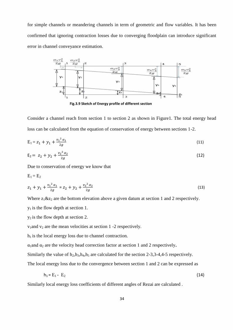
Fig.3.9 Sketch of Energy profile of different section

Consider a channel reach from section 1 to section 2 as shown in Figure1. The total energy head

loss can be calculated from the equation of conservation of energy between sections 1-2.

E1 =

(11)

E2

(12)

Due to conservation of energy we know that

E1 = E2

=

(13)

Where z1&z2 are the bottom elevation above a given datum at section 1 and 2 respectively.

y1 is the flow depth at section 1.

y2 is the flow depth at section 2.

v1and v2 are the mean velocities at section 1 -2 respectively.

h1 is the local energy loss due to channel contraction.

α1and α2 are the velocity head correction factor at section 1 and 2 respectively.

Similarly the value of h2,h3,h4,h5 are calculated for the section 2-3,3-4,4-5 respectively.

The local energy loss due to the convergence between section 1 and 2 can be expressed as

h1 = E1 - E2 (14)

Similarly local energy loss coefficients of different angles of Rezai are calculated .

35

3.4.3.1 SELECTION OF HYDRAULIC PARAMETERS FOR ENERGY LOSS

Flow hydraulics and momentum exchange in converging compound channels are significantly

influenced by both geometrical and hydraulic variables , the computation become more complex

when the floodplain width contracted and become zero. The flow factor responsible for the

estimation of energy losses are

i. Converging angle denoted as θ

ii. Width ratio(α)i.e.ratio of width of floodplain to width of main channel

iii. Aspect ratio(σ)i.e.ratio of width of main channel to depth of main channel

iv. Depth ratio Dr=(H-h)/H. H(height of water at a particular section),

h(height of water in main channel)

v. Relative distance (zr)i.e position of point velocity in the length wise direction of the

channel)/total length of the non-prismatic channel.

Hence in this study these five flow variables are chosen as input parameters and energy as output

parameter.

3.4.4 SHEAR STRESS MEASUREMENTS

Shear studies in open channel flow has many implications such as bed load transport, channel

migration, momentum transfer etc. Bed shear forces are useful for the study of bed load transfer

where as wall shear forces presents a general view of channel migration pattern. There are several

methods used to evaluate bed and wall shear stress in an open channel. The Preston-tube method is

an indirect estimate for shear stress measurements and is widely used for experimental channel

which is described below. In the following section, results regarding the distribution of boundary

shear stress along with the contours of local shear stress is shown and discussed. Also the mean

boundary shear stress results are discussed in details.

36

3.4.4.1 Methods for estimation of Boundary shear stress

Using Preston’s technique (1954) together with calibration curves of Patel’s (1965) local boundary

shear stress measurements were made around wetted perimeter of the present converging channel.

Preston developed a simple shear stress measurement technique for smooth boundaries in a fully

developed turbulent flow using a Pitot tube. Based on the law of the wall assumption (Bradshaw

and Huang, 1995), i.e. the velocity distribution near the wall can be empirically related to the

differential pressure between the dynamic and static pressures, Preston presented a non-dimensional

relationship between the differential pressures, P and the boundary shear stress,o

= [

] (15)

Where, d is the outside diameter of the tube, ρ is the density of the flow, ν is the kinematic

viscosity of the fluid and F is an empirical function. Following this work, Patel (1965) presented

definitive calibration curves for the Preston tube defined in terms of two non-dimensional

parameters which are used to convert pressure readings to boundary shear stress:

(

) (16) (

) (17)

The calibration of x*and y* for different regions of the velocity distribution (i.e. viscous sub

layer, buffer layer and logarithmic layer) is expressed by three different formulae

for (18)

for (19)

( ) for (20)

In the present case, all shear stress measurements are taken at all the five sections of the converging

angles. The pressure readings were taken using Pitot tube. These are placed at the predefined points

37

of the flow-grid in the channel, facing the flow. The manometers attached to the respective Pitot

tubes are used to measure head difference. The differential pressure was then calculated from the

readings on the vertical manometer:

P = gh (21)

Where h is the difference between the two readings from the dynamic and static, g is the

acceleration due to gravity and ρ is the density of water. Here the tube coefficient is taken as unit

and the error due to turbulence considered negligible while measuring velocity.

3.4.4.2 Selection of hydraulic parameters for Boundary Shear Stress

Selection of the currect hudraulic parameter for the Computation of the Boundary Shear Stress

generated at the walls of the non-prismatic sections throughout the compound channel is essential.

The flow factors responsible for the estimation of boundary shear stress and depth average velocity

are:

i. Converging angle denoted as θ

ii. Width ratio (α) i.e .ratio of width of floodplain to width of main channel

iii. Aspect ratio (σ) i.e. ratio of width of main channel to depth of main channel

iv. Depth ratio (β) = (H-h)/H. where H=height of water at a particular section and, h= height

of water in main channel

v. Relative distance (Zr) i.e of point velocity in the length wise direction of the channel)/total

length of the non-prismatic channel. Total five flow variables were chosen as input

parameters and energy as output parameter

38

3.4.5 MEASUREMENT OF BED SLOPE

Measuring the bed slope of the flume, there are several methods exists which are used according

to the practical conditions and researcher’s interest. Here in our present study we measured the

bed slope through water level piezometric tube. So first of all we took the water level with

reference to the bed of the channel at the upstream side and then downstream side of the

non-prismatic channel which is 15m apart. Here the level is taken from the bottom of the bed

excluding the Perspex sheet thickness. After taking the level at the two points, the difference in

the corresponding level was measured. The bed slope of the channel is calculated by dividing

this with the length of the channel. For more accuracy this procedure was continuing for three

times and the average was taken as the bed slope of 0.0011 for 5º converging compound channel

and 0.0017 for 12.38º converging compound channel.

39

CHAPTER 4

RESULTS

40

4.1 OVERVIEW

In chapter 3 the experimental procedures has been described with the outlines are given for the

experimental procedure carried out on the series of the tests. This chapter will now present the results of

these tests in terms of the Depth average velocity distributions, Energy stored throughout the

experimental sections and the energy loss between the experimental sections of a non-prismatic compound

channe and also the Boundary Shear stress generated in each section of the non-prismatic comoound channel.

The laboratory measurements were taken, readings have been recorded for all the sections of the non-

prismatic compound channel individually for all of the above mentioned studies taken into account for this

research work. After obtaining the records and the readings from the experimental work, analytical work was

performed of the data. Conventional methods have been used for each single aspect, tables have been

arranged and overall conventional techniques have been used to find out the results.

After finding out the results in the old conventional methods for Depth average velocity, Energy and Energy

loss calculations and the Boundary Shear distribution for the non-prismatic compound channel, an Adaptive

method has been used for ease of work. Artificial Neural Network has been used to find out or to predict the

results for the above mentioned aspects of flow and it has been seen that less amount of time has been taken

and accurate results have also been found in comparison to that of the old conventional techniques. A

comparison has also been made between the actual experimental data results or in simple words the target

values and the predicted values obtained by ANN technique and have been compared. The error in

calculations have also been compared and shown in this research work.

41

4.2 DEPTH AVERAGE VELOCITY RESULTS:

Depth-averaged velocity means the average velocity for a depth ‘h’ is assumed to occur at a height of 0.4h

from the bed level. Distribution of flow velocity in longitudinal and lateral direction is one of the important

aspects in open channel flows. It directly relates to numerous flow features like water profile estimation, shear

stress distribution, secondary flow, channel conveyance and host to other flow entities.

The depth average velocity measurements have been taken at 5 consecutive sections for the two channels of 5

and 13.38 degrees of the non-prismatic compound channels constructed in the Hydraulics laboratory of the

National Institute of Technology Rourkela.

Data from the studies of Bahram Rezai(2006) conducted on the non-prismatic reach of a compound channel

has also been taken into considerations. The depth-averaged velocity distribution within the cross-section was

measured at three positions for the 2m converging case (x=12m, x=13m, and x=14m) and five positions for

the 6m narrowing cases (x=8m, x=9.5m, x=llm, x=12.5m, and x=14m) for each relative depth.

In this part of the study, the adaptive technique of Artificial Neural Network has been used to predict he

Depth average velocity distribution along the non-prismatic reach of a compound channel.

A total of 19648 data points were gathered including the input and target parameters of which 17192 data

points were the Input parameters and 2456 data points were the Output of the Target points or values.

70% of the input and target values have been taken as the Training data set for the current network and the

remaining 30 % of the input and target parameters has been taken as the Testing data set for the current

Network, which means that 12035 data points from the input parameters have been assigned as the training

data set and 5157 data points have been assigned as the training data set for the Input Parameters, also 1720

data were assigned as the training data set for the target values and the remaining 736 data points were

assigned as the testing data set for the target values.

The analysis was performed in a Pentium 4 processor computer with the Matlab2010 software.

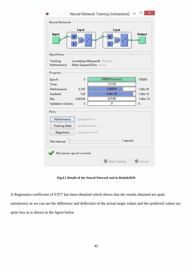
42

Fig.4.1 Details of the Neural Network tool in Matlab2010

A Regression coefficient of 0.977 has been obtained which shows that the results obtained are quite

satisfactory as we can see the difference and deflection of the actual target values and the predicted values are

quite less as is shown in the figure below

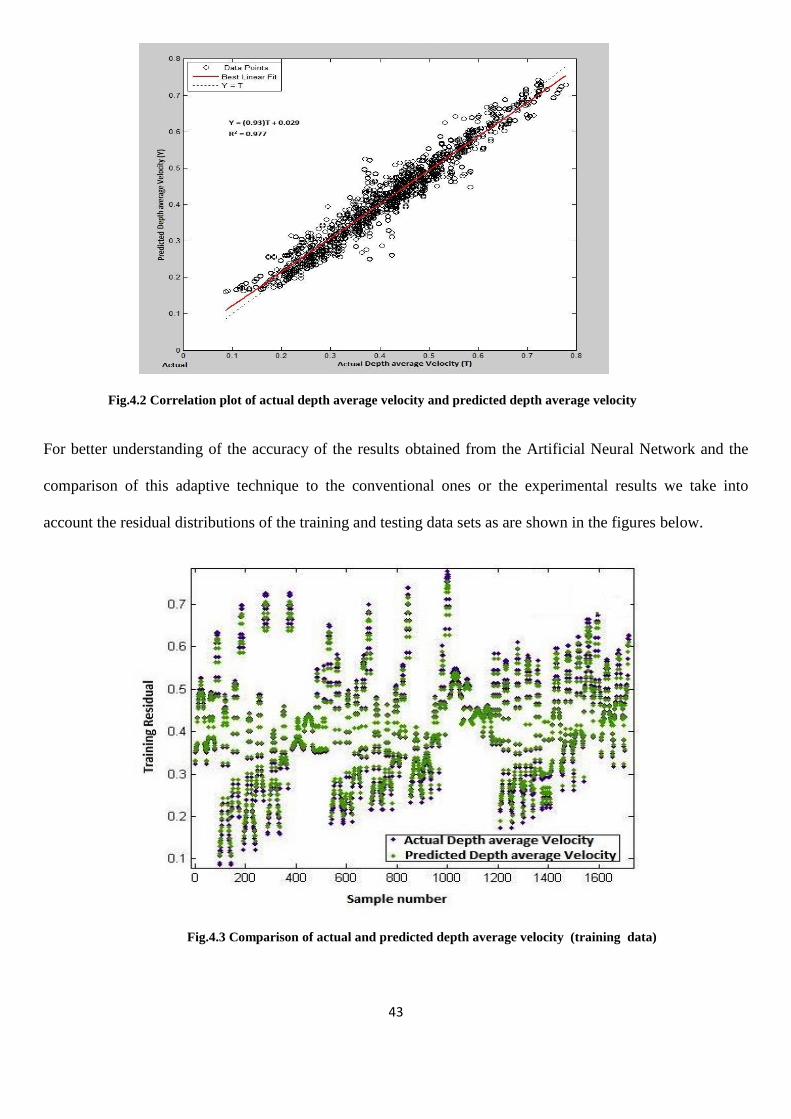
43

Fig.4.2 Correlation plot of actual depth average velocity and predicted depth average velocity

For better understanding of the accuracy of the results obtained from the Artificial Neural Network and the

comparison of this adaptive technique to the conventional ones or the experimental results we take into

account the residual distributions of the training and testing data sets as are shown in the figures below.

Fig.4.3 Comparison of actual and predicted depth average velocity (training data)

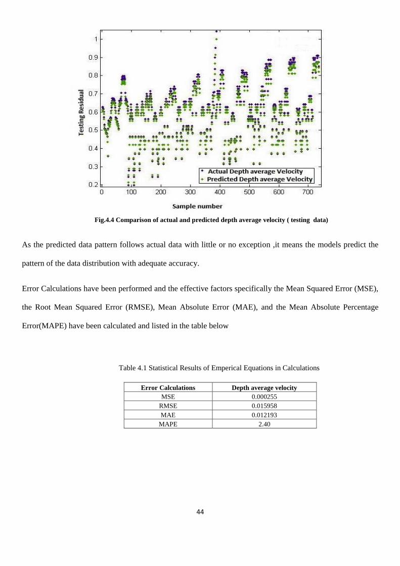
44

Fig.4.4 Comparison of actual and predicted depth average velocity ( testing data)

As the predicted data pattern follows actual data with little or no exception ,it means the models predict the

pattern of the data distribution with adequate accuracy.

Error Calculations have been performed and the effective factors specifically the Mean Squared Error (MSE),

the Root Mean Squared Error (RMSE), Mean Absolute Error (MAE), and the Mean Absolute Percentage

Error(MAPE) have been calculated and listed in the table below

Table 4.1 Statistical Results of Emperical Equations in Calculations

Error Calculations Depth average velocity

MSE 0.000255

RMSE 0.015958

MAE 0.012193

MAPE 2.40

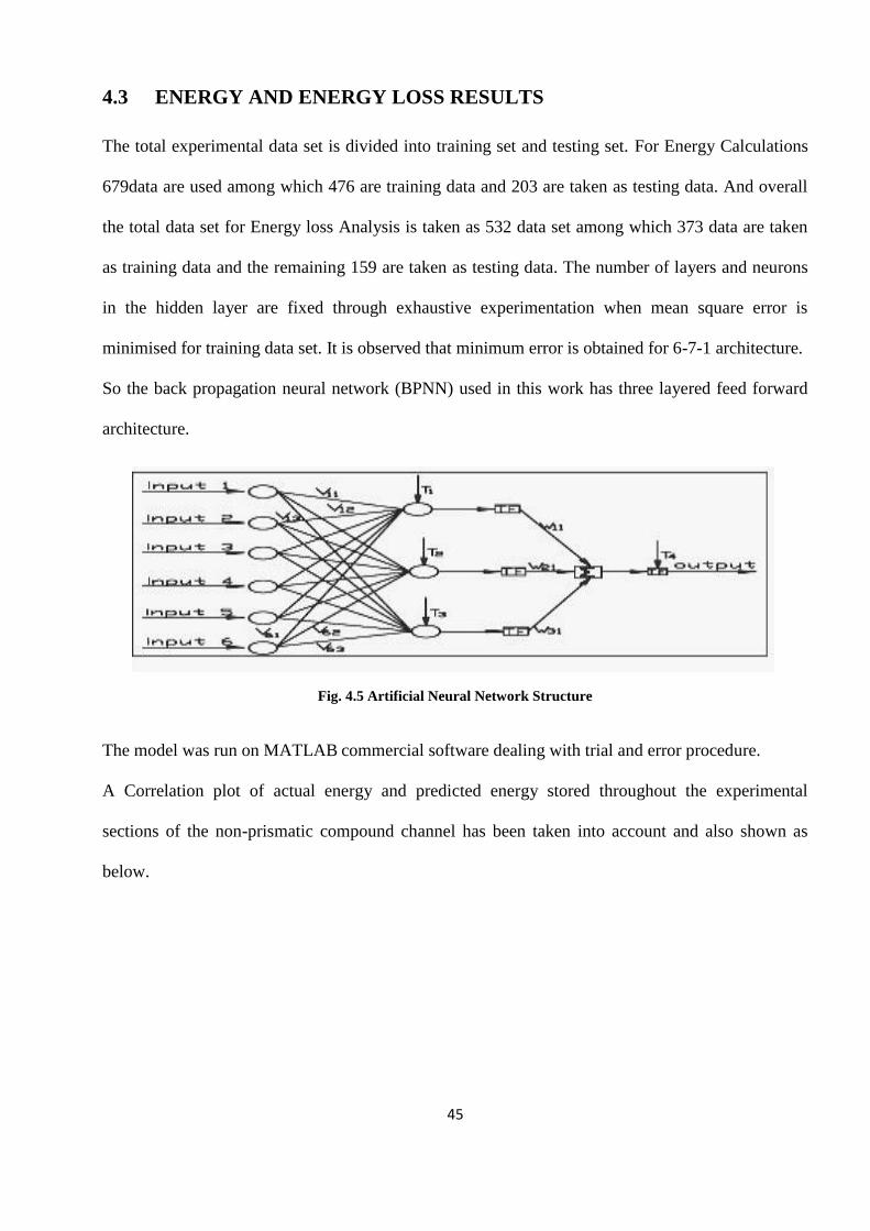
45

4.3 ENERGY AND ENERGY LOSS RESULTS

The total experimental data set is divided into training set and testing set. For Energy Calculations

679data are used among which 476 are training data and 203 are taken as testing data. And overall

the total data set for Energy loss Analysis is taken as 532 data set among which 373 data are taken

as training data and the remaining 159 are taken as testing data. The number of layers and neurons

in the hidden layer are fixed through exhaustive experimentation when mean square error is

minimised for training data set. It is observed that minimum error is obtained for 6-7-1 architecture.

So the back propagation neural network (BPNN) used in this work has three layered feed forward

architecture.

Fig. 4.5 Artificial Neural Network Structure

The model was run on MATLAB commercial software dealing with trial and error procedure.

A Correlation plot of actual energy and predicted energy stored throughout the experimental

sections of the non-prismatic compound channel has been taken into account and also shown as

below.

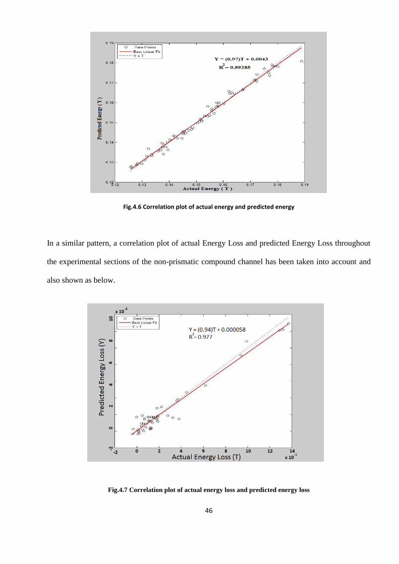
46

Fig.4.6 Correlation plot of actual energy and predicted energy

In a similar pattern, a correlation plot of actual Energy Loss and predicted Energy Loss throughout

the experimental sections of the non-prismatic compound channel has been taken into account and

also shown as below.

Fig.4.7 Correlation plot of actual energy loss and predicted energy loss

47

A regression curve is plotted between actual and predicted Energy and Energy Loss data which are

shown in figures above. It can be observed that data for both cases are well fitted because a high

degree of coefficient of determination R2 of 0.993 is obtained for the Energy Calculations and R

2 of

0.977 is obtained for the Energy Loss Analysis between the sections.

The residual analysis are carried out by calculating the residuals from the actual energy loss and

predicted energy loss data. The residual testing and training data are plotted against the sample

number as shown in fig (4.8) and fig (4.9), which shows that the residuals are distributed evenly

along the centerline of the plot. From this it can be said that the data are well trained.

As the predicted data pattern follows actual data with little or no exception ,it means the models

predict the pattern of the data distribution with adequate accuracy.

Fig.4.8 Residual distribution of training data of energy loss

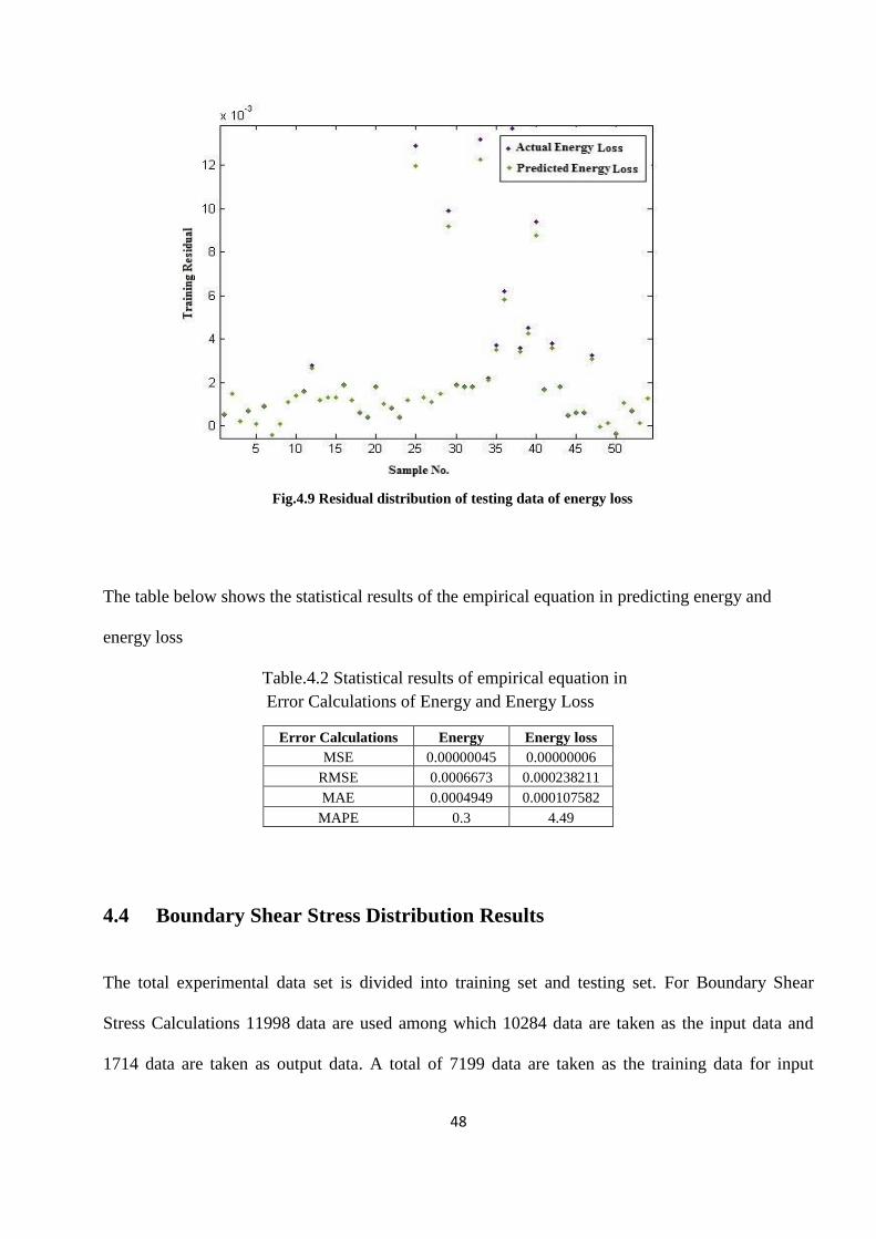
48

The table below shows the statistical results of the empirical equation in predicting energy and

energy loss

Table.4.2 Statistical results of empirical equation in

Error Calculations of Energy and Energy Loss

4.4 Boundary Shear Stress Distribution Results

The total experimental data set is divided into training set and testing set. For Boundary Shear

Stress Calculations 11998 data are used among which 10284 data are taken as the input data and

1714 data are taken as output data. A total of 7199 data are taken as the training data for input

Error Calculations Energy Energy loss

MSE 0.00000045 0.00000006

RMSE 0.0006673 0.000238211

MAE 0.0004949 0.000107582

MAPE 0.3 4.49

Fig.4.9 Residual distribution of testing data of energy loss

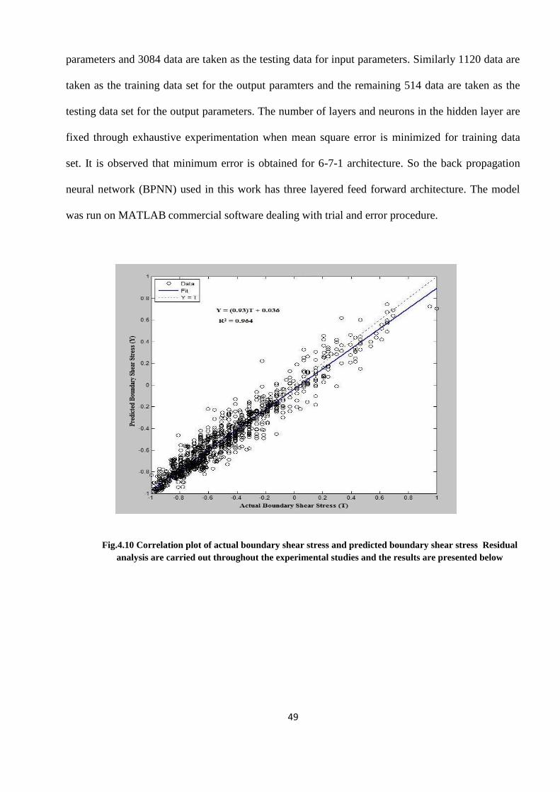
49

parameters and 3084 data are taken as the testing data for input parameters. Similarly 1120 data are

taken as the training data set for the output paramters and the remaining 514 data are taken as the

testing data set for the output parameters. The number of layers and neurons in the hidden layer are

fixed through exhaustive experimentation when mean square error is minimized for training data

set. It is observed that minimum error is obtained for 6-7-1 architecture. So the back propagation

neural network (BPNN) used in this work has three layered feed forward architecture. The model

was run on MATLAB commercial software dealing with trial and error procedure.

Fig.4.10 Correlation plot of actual boundary shear stress and predicted boundary shear stress Residual

analysis are carried out throughout the experimental studies and the results are presented below

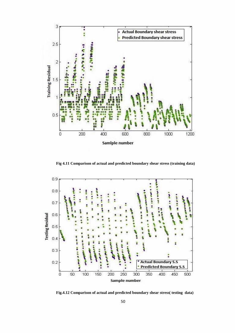
50

Fig 4.11 Comparison of actual and predicted boundary shear stress (training data)

Fig.4.12 Comparison of actual and predicted boundary shear stress( testing data)

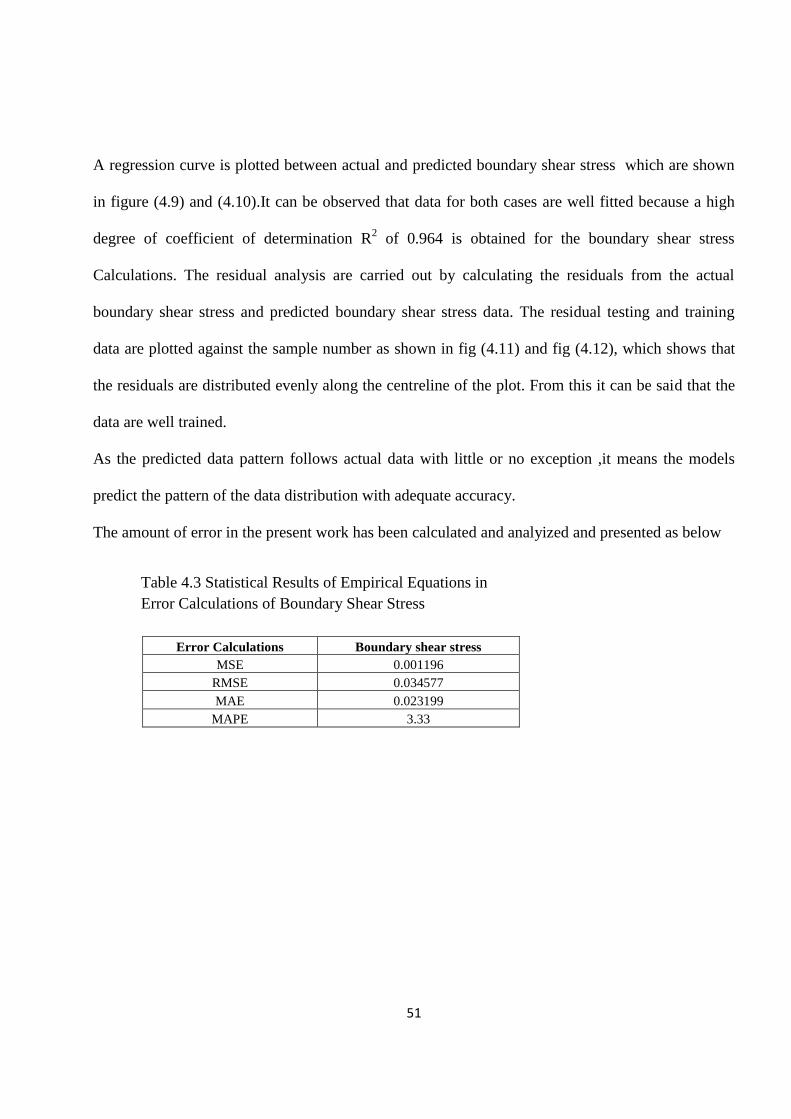
51

A regression curve is plotted between actual and predicted boundary shear stress which are shown

in figure (4.9) and (4.10).It can be observed that data for both cases are well fitted because a high

degree of coefficient of determination R2 of 0.964 is obtained for the boundary shear stress

Calculations. The residual analysis are carried out by calculating the residuals from the actual

boundary shear stress and predicted boundary shear stress data. The residual testing and training

data are plotted against the sample number as shown in fig (4.11) and fig (4.12), which shows that

the residuals are distributed evenly along the centreline of the plot. From this it can be said that the

data are well trained.

As the predicted data pattern follows actual data with little or no exception ,it means the models

predict the pattern of the data distribution with adequate accuracy.

The amount of error in the present work has been calculated and analyized and presented as below

Table 4.3 Statistical Results of Empirical Equations in

Error Calculations of Boundary Shear Stress

Error Calculations Boundary shear stress

MSE 0.001196

RMSE 0.034577

MAE 0.023199

MAPE 3.33

52

CHAPTER 5

CONCLUSIONS

53

SUMMARY:

The present theoretical investigation supported by experimental observation is made for Non-

prismatic compound channels with floodplains having different flow aspect ratios. On thevbasis of

the investigations concerning the non-prismatic reach of a compound channel to find out the Depth

average velocity, Energy stored and Energy lost throughout the experimental sections and the

Boundary shear stress developed throughout the experimental sections. flow, the following

conclusions are drawn.

Five different types of straight compound channel configurations have been investigated

Experimentally. Compound channels with non-prismatic floodplains, converging from 400mm to

0mm along 2m and 6m lengths and narrowing from 400mm to 200 mm along a 6m length.also two

of the compound channels constructed in the hydraulics laboratory of National Institute of

Technology Rourkela with the respective angles of 5 and 13.36 degrees. The specific objectives of

the experimental research programme, have been completed successfully. In this Chapter the main

conclusions of this research are presented

54

CONCLUSIONS:

1. Selection of depth average velocity of converging compound channels are found to depends

upon a numbers of hydraulic and geometric parameters out of which aspect ratio, depth

ratio, width ratio, relative distance, converging angle and relative depth are the most

influencing parameters.

2. An ANN model is proposed for accurate estimation of depth average velocity of converging

compound channels. The trend and pattern of experimental data matches with predicted

energy loss. The basic reason of high degree of prediction accuracy lies in the fact of

capability of nonlinear mapping of inputs and outputs in a Neural Network system. The

nonlinear relation of geometrical and hydraulic input parameters with and depth average

velocity data are difficult to establish with traditional depth average velocity data prediction

methodology. In addition, the conventional techniques cannot be taken into account the real

life factors operating in the system. It can be inferred that this model is more adaptive to the

prediction of boundary shear stress and depth average velocity under different conditions.

3. ANN model holds for depth average velocity MSE as 0.00025, RMSE as0.015958, MAE as

0.012193 and MAPE 2.40. So the present ANN model is more convincing model.

4. From the experimental results on converging compound channels, it is seen that the energy

loss between two sections at the binging is higher than that in later sections. This gradually

decreases and reaches minimum just before the mid of converging section. After reaching

minimum, there is a gradual increase trend is observed. This may be due to that at the entry

section there is a huge loss of energy because of sudden contraction from prismatic part to

55

non-prismatic part. After that the flow gets a transition reducing the loss and it is believed

that the transition is complete before mid-section.

5. In the lower width ratio converging experimental channels energy loss is higher at initial

overbank flow depths then the loss decreases and reaches minimum at the end of non-

prismatic section. This is because the present lower wide floodplain converging compound

channels have a shorter reach as compared to other higher width ratio channels.

6. Selection of energy loss of converging compound channels are found to depends upon a

numbers of hydraulic and geometric parameters out of which aspect ratio, depth ratio, width

ratio, relative distance, converging angle and relative depth are the most influencing

parameters.

7. An ANN model is proposed for accurate estimation of energy loss of converging compound

channels. The trend and pattern of experimental data matches with predicted energy loss.

The basic reason of high degree of prediction accuracy lies in the fact of capability of

nonlinear mapping of inputs and outputs in a Neural Network system. The nonlinear relation

of geometrical and hydraulic input parameters with energy loss is difficult to establish with

traditional energy loss prediction methodology. In addition, the conventional techniques

cannot be taken into account the real life factors operating in the system.it can be inferred

that this model is more adaptive to the prediction of energy loss under different conditions.

8. ANN model holds the energy loss prediction with minimal error i.e.MSE as 0.00000006

RMSE as0.000238211 MAE as0.000107582 and MAPE 4.49 which less than 10%..

Similarly for energy MSE as 0.00000045 RMSE as0.0006673 MAE as 0.0004949 and

56

MAPE 0.3. So the present ANN model is more convincing model.

9. Selection of boundary shear stress of converging compound channels are found to depends

upon a numbers of hydraulic and geometric parameters out of which aspect ratio, depth

ratio, width ratio, relative distance, converging angle and relative depth are the most

influencing parameters.

10. An ANN model is proposed for accurate estimation of boundary shear stress of converging

compound channels. The trend and pattern of experimental data matches with predicted

energy loss. The basic reason of high degree of prediction accuracy lies in the fact of

capability of nonlinear mapping of inputs and outputs in a Neural Network system. The

nonlinear relation of geometrical and hydraulic input parameters with boundary shear stress

data are difficult to establish with traditional boundary shear stress data prediction

methodology. In addition, the conventional techniques cannot be taken into account the real

life factors operating in the system. It can be inferred that this model is more adaptive to the

prediction of boundary shear stress under different conditions.

11. ANN model holds the boundary shear stress prediction with minimal error i.e.MSE as

0.001196 RMSE as0.034577 MAE as0.023199 and MAPE 3.33which less than 10%.

57

REFERENCES

58

B. Naik1, K.K.Khatua (2013), “Energy losses in a converging compound channel”,

Conference on Hydraulics, Water Resources ,Coastal & Environmental Engineering

Hydro-2013 International Organized by IIT Madras ,Chennai 600036,India.

B. Naik,, Khatua, K. K., Sahoo, R., & Satapathy, S. S. (2014). Flow Analysis for a

Converging Compound Channel. International Journal of Applied Engineering

Research, 9(2), 133-138.

Bilgil, A., & Altun, H. (2008). Investigation Of Flow Resistance In Smooth Open

Channels Using Artificial Neural Networks. Flow Measurement And

Instrumentation, 19(6), 404-408.

Barenblatt, G. I., & Prostokishin, V. M. (1993). Scaling laws for fully developed

turbulent shear flows. Part 2. Processing of experimental data. Journal of Fluid

Mechanics, 248, 521-529.

Bousmar, D., & Zech, Y. (2002). Discussion Of Two-Dimensional Solution For Straight

And Meandering Overbank Flows By D. Alan Ervine, K. Babaeyan-Koopaei, And

Robert HJ Sellin. Journal Of Hydraulic Engineering, 128(5), 550-551.

Bousmar, D., Wilkin, N., Jacquemart, J. H., & Zech, Y. (2004). Overbank Flow In

Symmetrically Narrowing Floodplains. Journal Of Hydraulic Engineering, 130(4), 305-

312.

Bousmar, D., 2001, "Flow modelling in compound channels - Momentum transfer

between main channel and prismatic or non-prismatic floodplains". PhD Thesis,

Universite Catholique de Louvain, Belgium.

Das, S. K., & Basudhar, P. K. (2006). Undrained Lateral Load Capacity Of Piles In Clay

Using Artificial Neural Network. Computers And Geotechnics, 33(8), 454-459.

Das, S. K., & Basudhar, P. K. (2008). Prediction Of Residual Friction Angle Of Clays

Using Artificial Neural Network. Engineering Geology, 100(3), 142-145.

59

Ghosh, S. N., & Mehta, P. (1974, March). Technical Note. Boundary Shear Distribution

In A Compound Channel With Varying Roughness Distribution. In Ice

Proceedings (Vol. 57, No. 1, Pp. 159-163). Thomas Telford.

Ghosh, S., & Jena, S. B. (1971, August). Boundary Shear Distribution In Open Channel

Compound. In ICE Proceedings (Vol. 49, No. 4, Pp. 417-430). Thomas Telford.

Ikeda, S., 1981, "Self-formed straight channels in sandy beds", Journal of Hydraulic

Division, ASCE, 107, HY4, April, 389-406.

Ikeda, S., 1999, "Role of lateral eddies in sediment transport and channel formation",

River Sedimentation, Jayawardena, Lee and Wang, eds., Balkema Rotterdam, 195-203.

Knight, D. W., & Demetriou, J. D. (1983). Flood Plain And Main Channel Flow

Interaction. Journal Of Hydraulic Engineering, 109(8), 1073-1092.

Knight, D.W. and Patel, H.S., (1985), “Boundary shear in smooth rectangular ducts”.

Journal of Hydraulic Engineering, ASCE, Vol. 111, No. 1, 29-47.

Knight, D. W., Demetriou, J. D., & Hamed, M. E. (1984). Boundary Shear In Smooth

Rectangular Channels. Journal Of Hydraulic Engineering, 110(4), 405-422.

Leal, J. G. A. B., Ferreira, R. M. L., Cardoso, A. H., Bousmar, D., & Zech, Y. (2002,

September). Dam-break waves on movable bed. In River Flow (pp. 981-990).

Meena, R. S., Jha, R., & Khatua, K. K. (2013). Precipitation-Runoff Simulation For A

Himalayan River Basin, India Using Artificial Neural Network Algorithms.Sciences In

Cold And Arid Regions, 5(1), 0085-0095.

Myers, R. C., & Elsawy, E. M. (1975). Boundary Shear In Channel With Flood

Plain. Journal Of The Hydraulics Division, 101(ASCE 11452 Proceeding).

Panda, P. (2010). Prediction Of Flow In Compound Open Channel Flows Using

60

Artificial Neural Network (Doctoral Dissertation).

Preston, J.H., 1954, "The determination of turbulent skin friction by means of Pitot

tubes", Journal Roy. Aero. Soc. Vol. 58, 109-121.

Proust, S., Bousmar, D., Rivière, N., Paquier, A., & Zech, Y. (2010). Energy Losses In

Compound Open Channels. Advances In Water Resources, 33(1), 1-16.

Proust, S., Rivière, N., Bousmar, D., Paquier, A., Zech, Y., & Morel, R. (2006). Flow In

Compound Channel With Abrupt Floodplain Contraction. Journal Of Hydraulic

Engineering, 132(9), 958-970.

Rajaratnam, N., & Ahmadi, R. M. (1979). Interaction Between Main Channel And

Flood-Plain Flows. Journal Of The Hydraulics Division, 105(5), 573-588.

Rezaei, B., & Knight, D. W. (2009). Application Of The Shiono And Knight Method In

Compound Channels With Non-Prismatic Floodplains. Journal Of Hydraulic

Research, 47(6), 716-726.

Rezaei, B. (2006). Overbank flow in compound channels with prismatic and non-

prismatic floodplains (Doctoral dissertation, University of Birmingham).

Sahu, M. (2011). Prediction Of Flow And Its Resistance In Compound Open

Channel (Doctoral Dissertation).

Schlichting, H. „1979, Boundary-Layer Theory.

Sellin, R. H. J. (1964). A laboratory investigation into the interaction between the flow

in the channel of a river and that over its flood plain. La Houille Blanche, (7), 793-802.

Sahu, M., Khatua, K. K., & Mahapatra, S. S. (2011). A Neural Network Approach For

61

Prediction Of Discharge In Straight Compound Open Channel Flow.Flow Measurement

And Instrumentation, 22(5), 438-446.

Prandtll. ,1926 Uberdie ausgebildete Turbulenz. In Proc. 2nd Znt. Kong.fiir Tech. Mech.,

Zurich.

Sahu, M., Singh, P., Mahapatra, S. S., & Khatua, K. K. (2012). Prediction Of Entrance

Length For Low Reynolds Number Flow In Pipe Using Neuro-Fuzzy Inference

System. Expert Systems With Applications, 39(4), 4545-4557.

Shayya, W. H., & Sablani, S. S. (1998). An artificial neural network for non-iterative

calculation of the friction factor in pipeline flow. Computers and electronics in

agriculture, 21(3), 219-228.

Tominaga, A., & Nezu, L. (1992). Velocity Profiles In Steep Open-Channel

Flows.Journal Of Hydraulic Engineering, 118(1), 73-90.

Wormleaton, P. R., Allen, J., & Hadjipanos, P. (1982). Discharge Assessment In

Compound Channel Flow. Journal Of The Hydraulics Division, 108(9), 975-994.

Yuhong, Z., & Wenxin, H. (2009). Application of artificial neural network to predict the

friction factor of open channel flow. Communications in Nonlinear Science and

Numerical Simulation, 14(5), 2373-2378.

Zahiri, A., & Dehghani, A. A. (2009). Flow discharge determination in straight

compound channels using ANN. World Acad Sci Eng Technol, 58, 1-8.

62

PUBLICATIONS:

B. Naik, K.K.Khatua, and Kamel Miri (2014) , “Prediction of Energy loss along the non-

prismatic reach of a compound channel using ANN” Proceedings of the international

conference on fluvial Hydraulics, Lausane, Switzerland.