Kaplan-Meier Estimator Nonparametric and Semi …kkoehler/stat565/kaplanmeier.4page.pdf · Nonparametric and Semi-parametric Methods • Estimate a survivor function without covariates:

Nonparametric andSemi-parametric Methods

• Estimate a survivor function without

covariates:

– Kaplan-Meier (product-limit)

Estimator

– Nelson-Aalen Estimator

– Life table estimator

• Estimate a survivor function with

covariates: Cox proportional hazards

model

220

Kaplan-Meier Estimator

• Also called the product-limit estimator

• Most commonly used estimator

• Suppose t(1) < t(2) < ... < t(r) are the

ordered failure times.

– Let nj denote the number of

individuals alive (at risk) just

before time t(j), including

those who will die at time t(j)

– If an observation is censored at the

same time t(j) that one or more

failures occur, then censoring is

assumed to occur after any failures

and nj includes the censored

observations

– Let dj denote the number of failures

(deaths) at time t(j)

221

– The conditional probability that an

individual dies in the time interval

from t(j) − ∆ to t(j), given survival

up to time t(j) − ∆, is estimated as

dj

nj

– The conditional probability that an

individual survives beyond t(j) − ∆,

given survival up to time t(j) − ∆, is

estimated as

nj − dj

nj

– In the limit as ∆ → 0,

nj − dj

nj

becomes an estimate of the condi-

tional probability of surviving beyond

t(j) given survival up to t(j).

• For t(k) ≤ t < t(k+1), the probability ofsurviving beyond time t is

S(t) = P{T > t} = P{T > t and T > t(k)}

= P{T > t|T > t(k)}P{T > t(k}

= P{T > t|T > t(k)}

×P{T > t(k)|T > t(k−1)}

×P{T > t(k−1)}

= P{T > t|T > t(k)}

×P{T > t(k)|T > t(k−1)}

×P{T > t(k−1)|T > t(k−2)}

× . . . × P{T > t(1)|T > t(0)}

×P{T > t(0)}

≈ k∏j=1

P{T > t(j)|T > t(j−1)}

where t(0) = 0 and t(r+1) = ∞

222

• The Kaplan-Meier estimator of the

survivor function at time t,

for t(k) ≤ t < t(k+1), is

S(t) =k∏

j=1

nj − dj

nj

223

Example:

Subject Time Failure1 6 12 8 03 12 14 3 15 21 16 12 1

Order with respect to failure times

j t(j) nj dj (nj − dj)/nj S(t)

0 0 6 0 1.0000 1.00001 3 6 1 0.8333 0.83332 6 5 1 0.8000 0.66673 12 3 2 0.3333 0.22224 21 1 1 0.0000 0.0000

224

Variance of the Kaplan-Meierestimator (Greenwood’s formula)

For t(k) ≤ t < t(k+1),

ˆV ar(S(t)) = (S(t))2k∑

j=1

dj

nj(nj − dj)

Derivation:

• Start with

log(S(t)) = log

⎛⎜⎜⎜⎝

k∏j=1

nj − dj

nj

⎞⎟⎟⎟⎠

=k∑

j=1log((nj − dj)/nj)

=k∑

j=1log(pj)

225

• Then

V ar(log(S(t)

)= V ar

⎛⎜⎜⎝

k∑j=1

log(pj)

⎞⎟⎟⎠

=k∑

j=1V ar

(log(pj)

)

• Apply the delta method

V ar(log(pj)

) ≈⎛⎜⎜⎜⎝

1

πj

⎞⎟⎟⎟⎠2 πj(1 − πj)

nj

=

⎛⎜⎜⎜⎝

1

πj

⎞⎟⎟⎟⎠1 − πj

nj

• Then

V ar(log(S(t)) ≈ k∑j=1

⎛⎜⎜⎜⎝

1

πj

⎞⎟⎟⎟⎠1 − πj

nj

226

• Apply the delta method a second time

to get

V ar(S(t)) ≈ [S(t)]2V ar(log(S(t))

)

= [S(t)]2k∑

j=1

⎛⎜⎜⎜⎝

1

πj

⎞⎟⎟⎟⎠1 − πj

nj

• The Greenwood formula, obtained by

substituting pj = (nj − dj)/nj for πj, is

ˆV ar(S(t)) = (S(t))2k∑

j=1

dj

nj(nj − dj)

• A large sample standard error for S(t)

is

se(S(t)) = S(t)

√√√√√√√√k∑

j=1

dj

nj(nj − dj)

227

Confidence intervals

• Large sample normal distribution for

S(t)

S(t) ± Zα/2S(t)

√√√√√√√√k∑

j=1

dj

nj(nj − dj)

potential problems:

– endpoints outside 0 or 1

– normality if sample size is not large

• CI based on the large sample normal

distribution of log[−log(S(t))] with

ˆV ar(log(−log(S(t)))

)=

(1/(log(S(t)))2) ∑kj=1

dini(ni−di)

for t(k) ≤ t ≤ t(k+1)

228

• Compute

L = log(−log(S(t))) − Zα/2

(1

log(S(t))

) √∑kj=1

di

ni(ni−di)

U = log(−log(S(t))) + Zα/2

(1

log(S(t))

) √∑kj=1

di

ni(ni−di)

• Back transform endpoints (L, U) to

obtain

(exp(− exp(U)), exp(− exp(L)))

229

Kaplan-Meier Estimator in SAS

/* SAS code for Kaplan-Meier estimation of

surviror functions to times from the VA

lung cancer trial of 137 male patients

with inoperable lung cancer. This code

is posted as vakm.sas */

/* Variables

Treatment: 1=standard, 2=test (chemotherapy)

Celltype: 1=squamous, 2=smallcell,

3=adeno, 4=large

Survival in days

Status: 1=dead, 0=censored

Karnofsky score

Months from Diagnosis

Age in years

Prior therapy: 0=no, 10=yes

*/

230

data va;

infile ’c:\stat565\va.dat’;

input rx cellt time status karno months

age prior_rx;

prior_rx = prior_rx/10;

if (cellt=1) then celltype= ’squamous’;

if (cellt=2) then celltype= ’smallcell’;

if (cellt=3) then celltype= ’adeno’;

if (cellt=4) then celltype= ’large’;

proc lifetest method=KM plots=(s) graphics

outs=su data=va;

time time*status(0);

strata rx;

symbol1 v=none color=black line=1;

symbol2 v=none color=black line=2;

run;

proc print data=su; run;

231

/* Delete censored cases */

data su2;

set su;

if _CENSOR_=0;

run;

goptions rotate=landscape;

axis1 label=(f=swiss h=1.2 a=90 r=0

"Survial Probability")

order = 0 to 1 by 0.1

length= 4.3in w=3

value=(f=swiss h=1.0);

axis2 label=(f=swiss h=1.2 "Time(days)")

order = 0 to 1000 by 100

value=(f=swiss h=1.0) w=3

length = 6. in;

232

proc gplot data=su2; by rx;

plot (SURVIVAL SDF_LCL SDF_UCL)*time/

overlay vaxis=axis1 haxis=axis2;;

symbol1 v=none interpol=join color=black

line=1 w=4;


line=3 w=4;


line=3 w=4;

title ls=0.4 H=2.0 F=swiss

"Estimated Survivor Function";

run;

233

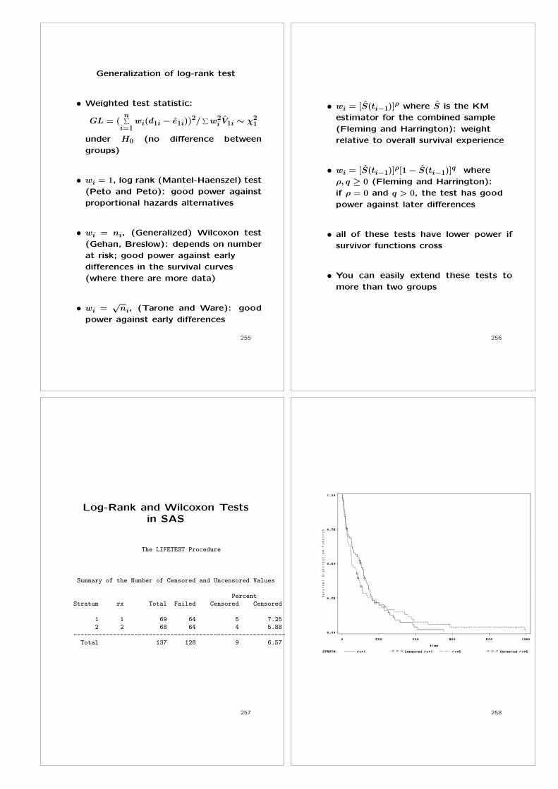
The LIFETEST ProcedureStratum 1: rx = 1

Product-Limit Survival Estimates

SurvivalStandard Number Number

time Survival Failure Error Failed Left0.000 1.0000 0 0 0 693.000 0.9855 0.0145 0.0144 1 684.000 0.9710 0.0290 0.0202 2 677.000 0.9565 0.0435 0.0246 3 668.000 . . . 4 658.000 0.9275 0.0725 0.0312 5 6410.000 . . . 6 6310.000 0.8986 0.1014 0.0363 7 6211.000 0.8841 0.1159 0.0385 8 6112.000 . . . 9 6012.000 0.8551 0.1449 0.0424 10 5913.000 0.8406 0.1594 0.0441 11 5816.000 0.8261 0.1739 0.0456 12 5718.000 . . . 13 5618.000 0.7971 0.2029 0.0484 14 5520.000 0.7826 0.2174 0.0497 15 5421.000 0.7681 0.2319 0.0508 16 5322.000 0.7536 0.2464 0.0519 17 5225.000* . . . 17 5127.000 0.7388 0.2612 0.0529 18 50

.

.

.411.000 0.0177 0.9823 0.0175 63 1553.000 0 1.0000 0 64 0

NOTE: The marked survival times are censored observations.

234

The LIFETEST Procedure

Summary Statistics for Time Variable time

Quartile Estimates

Point 95% Confidence IntervalPercent Estimate [Lower Upper)

75 162.000 132.000 250.00050 103.000 56.000 126.00025 27.000 16.000 54.000

Mean Standard Error

123.928 14.961

235

The LIFETEST ProcedureStratum 2: rx = 2

Product-Limit Survival Estimates

SurvivalStandard Number Number

time Survival Failure Error Failed Left

0.000 1.0000 0 0 0 681.000 . . . 1 671.000 0.9706 0.0294 0.0205 2 662.000 0.9559 0.0441 0.0249 3 657.000 . . . 4 647.000 0.9265 0.0735 0.0317 5 638.000 . . . 6 628.000 0.8971 0.1029 0.0369 7 6113.000 0.8824 0.1176 0.0391 8 6015.000 . . . 9 5915.000 0.8529 0.1471 0.0429 10 5818.000 0.8382 0.1618 0.0447 11 57

.

.

.467.000 0.0549 0.9451 0.0303 61 3587.000 0.0366 0.9634 0.0251 62 2991.000 0.0183 0.9817 0.0180 63 1999.000 0 1.0000 0 64 0

NOTE: The marked survival times are censored observations.

236

Summary Statistics for Time Variable time

Quartile Estimates

Point 95% Confidence IntervalPercent Estimate [Lower Upper)

75 140.000 95.000 283.00050 52.500 44.000 90.00025 24.500 19.000 36.000

Mean Standard Error

142.061 27.023

Summary of the Number of Censored and Uncensored Values

PercentStratum rx Total Failed Censored Censored

1 1 69 64 5 7.252 2 68 64 4 5.88

-----------------------------------------------------------Total 137 128 9 6.57

237 238

Testing Homogeneity of Survival Curves over Strata

Rank Statistics

rx Log-Rank Wilcoxon

1 -0.50020 -447.00

2 0.50020 447.00

Test of Equality over Strata

Pr >

Test Chi-Square DF Chi-Square

Log-Rank 0.0082 1 0.9277

Wilcoxon 0.9608 1 0.3270

-2Log(LR) 0.2758 1 0.5995

239

Output created by the outs= option

Obs rx time _CENSOR_ SURVIVAL SDF_LCL SDF_UCL STRATUM

1 1 0 0 1.00000 1.00000 1.00000 12 1 3 0 0.98551 0.95731 1.00000 13 1 4 0 0.97101 0.93143 1.00000 14 1 7 0 0.95652 0.90840 1.00000 15 1 8 0 0.92754 0.86636 0.98871 16 1 10 0 0.89855 0.82731 0.96979 1

18 1 31 0 0.70929 0.60194 0.81665 1...

62 1 411 0 0.01770 0.00000 0.05197 163 1 553 0 0.00000 0.00000 0.00000 164 2 0 0 1.00000 1.00000 1.00000 265 2 1 0 0.97059 0.93043 1.00000 266 2 2 0 0.95588 0.90707 1.00000 267 2 7 0 0.92647 0.86444 0.98851 2...

117 2 587 0 0.03659 0.00000 0.08581 2118 2 991 0 0.01830 0.00000 0.05363 2119 2 999 0 0.00000 0.00000 0.00000 2

240

241 242

Kaplan-Meier Estimation in R orSPlus

# R code to estimate the survivor

# function for the VA lung cancer trial

# of 137 male patients with inoperable

# lung cancer. This code is posted as

# vakm.ssc

# Variables

# Treatment: 1=standard, 2=test (chemotherapy)

# Celltype: 1=squamous, 2=smallcell,

# 3=adeno, 4=large

# Survival in days

# Status: 1=dead, 0=censored

# Karnofsky score

# Months from Diagnosis

# Age in years

# Prior therapy: 0=no, 10=yes

# Enter the data into a data frame.

243

va <- read.table("c:/va.dat",

header=F, col.names=c("rx", "cellt", "time",

"status", "karno", "months", "age",

"prior_rx"))

va$prior_rx <- va$prior_rx/10;

va

rx cellt time status karno months age prior_rx

1 1 1 72 1 60 7 69 0

2 1 1 411 1 70 5 64 10

3 1 1 228 1 60 3 38 0

4 1 1 126 1 60 9 63 10

5 1 1 118 1 70 11 65 10

.

.

.

134 2 4 111 1 60 5 64 0

135 2 4 231 1 70 18 67 10

136 2 4 378 1 80 4 65 0

137 2 4 49 1 30 3 37 0

244

vafit <- survfit(Surv(time, status) ~ rx,

data = va,

conf.int=.95, conf.type="log-log",

type="kaplan-meier", se.fit=T)

# Specify the type of survival curve estimator.

# Possible values are

# "kaplan-meier", "fleming-harrington" or "fh2"

# if a formula is given and

# "aalen" or "kaplan-meier"

# if the first argument is a coxph object (only the

# first two characters are necessary). The default

# is "aalen" when a coxph object is given, and

# it is "kaplan-meier" otherwise.

# conf.type: specifies the confidence interval

# type. Possible values are:

# "none" for no confidence intervals

# "plain" for standard intervals,

# "curve +- k*se(curve)", where k

# is determined from conf.int,

# "log" for intervals based on the cumulative

# hazard or log(survival) (the default)

245

# "log-log" for intervals based on the log

# hazard or log(-log(survival)).

# The last type will never extend past 0 or 1.

# Print out estimates of median survival times

vafit

Call: survfit(formula = Surv(time, status) ~ rx,

data = va, conf.int = 0.95,

conf.type = "log-log",

type = "kaplan-meier", se.fit = T)

n events mean se(mean) median 0.95LCL 0.95UCL

rx=1 69 64 124 14.8 103 54 126

rx=2 68 64 142 26.8 52 43 90

# Print out estimates of survivor curve and

# confidence limits

summary(vafit)

246

rx=1time n.risk n.event survival std.err lower 95% CI upper 95% CI

3 69 1 0.986 0.0144 0.958 1.0004 68 1 0.971 0.0202 0.932 1.0007 67 1 0.957 0.0246 0.910 1.0008 66 2 0.928 0.0312 0.868 0.99110 64 2 0.899 0.0363 0.830 0.97311 62 1 0.884 0.0385 0.812 0.96312 61 2 0.855 0.0424 0.776 0.942...

392 3 1 0.0354 0.0244 0.00917 0.137411 2 1 0.0177 0.0175 0.00256 0.123553 1 1 0.0000 NA NA NA

rx=2time n.risk n.event survival std.err lower 95% CI upper 95% CI

1 68 2 0.971 0.0205 0.931 1.0002 66 1 0.956 0.0249 0.908 1.0007 65 2 0.926 0.0317 0.866 0.9918 63 2 0.897 0.0369 0.828 0.97213 61 1 0.882 0.0391 0.809 0.96215 60 2 0.853 0.0429 0.773 0.94118 58 1 0.838 0.0447 0.755 0.930...

467 4 1 0.0549 0.0303 0.01861 0.162587 3 1 0.0366 0.0251 0.00953 0.140991 2 1 0.0183 0.0180 0.00265 0.126999 1 1 0.0000 NA NA NA

247

plot(vafit, lty = 2:3, lwd=4, cex=3)

legend(400, .8, c("Standard", "Chemotherapy"),

lty = 2:3)

0 200 400 600 800 1000

0.0

0.2

0.4

0.6

0.8

1.0

StandardChemotherapy

248

Life-Table Estimator

• Grouped data (interval censoring)

analog of the Kaplan-Meier estimator

• Survival data generally presented in

calendar time units (monthly, semi-

annually, etc.)

• Suppose we use 6 month intervals,

[t, t+6): n= number of subjects at risk

of dying at time t; d subjects die in the

interval; c subjects are censored during

the interval

• Conditional probability of surviving

during the interval is

(n − (c/2) − d)/(n − (c/2))

c/2 correction assumes that censored

observations are uniformly distributed

over the interval

249

• Example:

Interval Enter Die Censored S[0, 6) 100 41 10 .5684[6, 12) 49 21 3 .3171[12, 18) 25 6 2 .2378[18, 24) 17 1 1 .2234

250

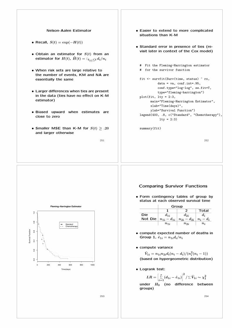
Nelson-Aalen Estimator

• Recall, S(t) = exp(−H(t))

• Obtain an estimator for S(t) from an

estimator for H(t), H(t) = ∑t(i)≤t di/ni

• When risk sets are large relative to

the number of events, KM and NA are

essentially the same

• Larger differences when ties are present

in the data (ties have no effect on K-M

estimator)

• Biased upward when estimates are

close to zero

• Smaller MSE than K-M for S(t) ≥ .20

and larger otherwise

251

• Easier to extend to more complicated

situations than K-M

• Standard error in presence of ties (re-

visit later in context of the Cox model)

# Fit the Fleming-Harrington estimator

# for the survivor function

fit <- survfit(Surv(time, status) ~ rx,

data = va, conf.int=.95,

conf.type="log-log", se.fit=T,

type="fleming-harrington")

plot(fit, lty = 2:3,

main="Fleming-Harrington Estimator",

xlab="Time(days)",

ylab="Survival Function")


lty = 2:3)

summary(fit)

252

0 200 400 600 800 1000

0.0

0.2

0.4

0.6

0.8

1.0

Fleming−Harrington Estimator

Time(days)

Sur

viva

l Fun

ctio

n


253

Comparing Survivor Functions

• Form contingency tables of group bystatus at each observed survival time

Group1 2 Total

Die d1i d2i diNot Die n1i − d1i n2i − d2i ni − di

n1i n2i ni

• compute expected number of deaths inGroup 1, e1i = n1idi/ni

• compute variance

V1i = n1in2idi(ni − di)/(n2i (ni − 1))

(based on hypergeometric distribution)

• Logrank test:

LR =⎡⎢⎣ r∑i=1

(d1i − e1i)⎤⎥⎦2

/∑

V1i ∼ χ21

under H0 (no difference betweengroups)

254

Generalization of log-rank test

• Weighted test statistic:

GL = (n∑

i=1wi(d1i − e1i))

2/∑

w2i V1i ∼ χ2

1

under H0 (no difference between

groups)

• wi = 1, log rank (Mantel-Haenszel) test

(Peto and Peto): good power against

proportional hazards alternatives

• wi = ni, (Generalized) Wilcoxon test

(Gehan, Breslow): depends on number

at risk; good power against early

differences in the survival curves

(where there are more data)

• wi =√

ni, (Tarone and Ware): good

power against early differences

255

• wi = [S(ti−1)]ρ where S is the KM

estimator for the combined sample

(Fleming and Harrington): weight

relative to overall survival experience

• wi = [S(ti−1)]ρ[1 − S(ti−1)]

q where

ρ, q ≥ 0 (Fleming and Harrington):

if ρ = 0 and q > 0, the test has good

power against later differences

• all of these tests have lower power if

survivor functions cross

• You can easily extend these tests to

more than two groups

256

Log-Rank and Wilcoxon Testsin SAS


Summary of the Number of Censored and Uncensored Values

PercentStratum rx Total Failed Censored Censored

1 1 69 64 5 7.252 2 68 64 4 5.88

-----------------------------------------------------------Total 137 128 9 6.57

257 258

Testing Homogeneity of Survival Curves over Strata

LOG RANK AND WILCOXON STATISTICS FOR EACH GROUP

NUMERATOR OF TEST STATISTIC

Rank Statistics

rx Log-Rank Wilcoxon

1 -0.50020 -447.00

2 0.50020 447.00

FOR TWO STRATA THE VALUES ARE PERFECTLY

CORRELATED, THEY SUM TO ZERO

Covariance Matrix for the Log-Rank Statistics

rx 1 2

1 30.4104 -30.4104

2 -30.4104 30.4104

259

Covariance Matrix for the Wilcoxon Statistics

rx 1 2

1 207972 -207972

2 -207972 207972


Pr >


Log-Rank 0.0082 1 0.9277

Wilcoxon 0.9608 1 0.3270

-2Log(LR) 0.2758 1 0.5995

Note: The likelihood ratio test assumes an

exponential distribution

260

Log-Rank Tests in R and SPlus

survdiff(Surv(time,status)~, data, rho=0)

This function implements the G-rho family of

Harrington and Fleming (1982), with weights

on each death of (S(t))^rho, where S is the

Kaplan-Meier estimate of the survivor function.

When rho = 0 this is the log-rank or

Mantel-Haenszel test, and when rho = 1 it

is equivalent to the Peto & Peto modification

of the Gehan-Wilcoxon test.

261

library(survival)

survdiff(Surv(time, status) ~ rx,

data=va, rho=0)

Call:

survdiff(formula = Surv(time, status) ~ rx,

data = va, rho = 0)

N Observed Expected (O-E)^2/E (O-E)^2/V

rx=1 69 64 64.5 0.00388 0.00823

rx=2 68 64 63.5 0.00394 0.00823

Chisq= 0 on 1 degrees of freedom, p= 0.928

262

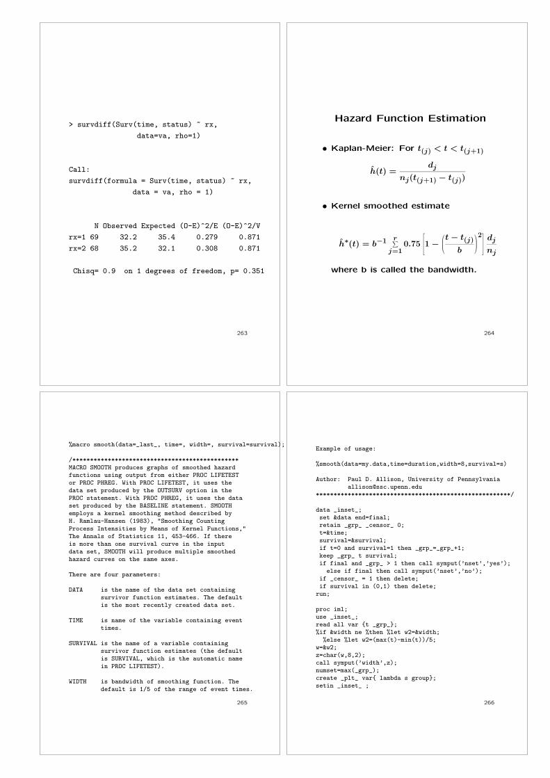
> survdiff(Surv(time, status) ~ rx,

data=va, rho=1)

Call:

survdiff(formula = Surv(time, status) ~ rx,

data = va, rho = 1)

N Observed Expected (O-E)^2/E (O-E)^2/V

rx=1 69 32.2 35.4 0.279 0.871

rx=2 68 35.2 32.1 0.308 0.871

Chisq= 0.9 on 1 degrees of freedom, p= 0.351

263

Hazard Function Estimation

• Kaplan-Meier: For t(j) < t < t(j+1)

h(t) =dj

nj(t(j+1) − t(j))

• Kernel smoothed estimate

h∗(t) = b−1 r∑j=1

0.75

⎡⎢⎢⎢⎣1 −

⎛⎜⎜⎝t − t(j)

b

⎞⎟⎟⎠2⎤⎥⎥⎥⎦dj

nj

where b is called the bandwidth.

264

%macro smooth(data=_last_, time=, width=, survival=survival);

/***********************************************MACRO SMOOTH produces graphs of smoothed hazardfunctions using output from either PROC LIFETESTor PROC PHREG. With PROC LIFETEST, it uses thedata set produced by the OUTSURV option in thePROC statement. With PROC PHREG, it uses the dataset produced by the BASELINE statement. SMOOTHemploys a kernel smoothing method described byH. Ramlau-Hansen (1983), "Smoothing CountingProcess Intensities by Means of Kernel Functions,"The Annals of Statistics 11, 453-466. If thereis more than one survival curve in the inputdata set, SMOOTH will produce multiple smoothedhazard curves on the same axes.

There are four parameters:

DATA is the name of the data set containingsurvivor function estimates. The defaultis the most recently created data set.

TIME is name of the variable containing eventtimes.

SURVIVAL is the name of a variable containingsurvivor function estimates (the defaultis SURVIVAL, which is the automatic namein PROC LIFETEST).

WIDTH is bandwidth of smoothing function. Thedefault is 1/5 of the range of event times.

265

Example of usage:

%smooth(data=my.data,time=duration,width=8,survival=s)

Author: Paul D. Allison, University of [email protected]

*******************************************************/

data _inset_;set &data end=final;retain _grp_ _censor_ 0;t=&time;survival=&survival;if t=0 and survival=1 then _grp_=_grp_+1;keep _grp_ t survival;if final and _grp_ > 1 then call symput(’nset’,’yes’);

else if final then call symput(’nset’,’no’);if _censor_ = 1 then delete;if survival in (0,1) then delete;run;

proc iml;use _inset_;read all var {t _grp_};%if &width ne %then %let w2=&width;%else %let w2=(max(t)-min(t))/5;

w=&w2;z=char(w,8,2);call symput(’width’,z);numset=max(_grp_);create _plt_ var{ lambda s group};setin _inset_ ;

266

do m=1 to numset;read all var {t survival _grp_} where (_grp_=m);n=nrow(survival);lo=t[1] + w;hi=t[n] - w;npt=50;inc=(hi-lo)/npt;s=lo+(1:npt)‘*inc;group=j(npt,1,m);slag=1//survival[1:n-1];h=1-survival/slag;x = (j(npt,1,1)*t‘ - s*j(1,n,1))/w;k=.75*(1-x#x)#(abs(x)<=1);lambda=k*h/w;append;

end;quit;

%if &nset = yes %then %let c==group;%else %let c=;

proc gplot data=_plt_;plot lambda*s &c / vaxis=axis1

vzero haxis=axis2;axis1 label=(angle=90 f=swiss h=2.5

’Hazard Function’ ) minor=none ;axis2 label=(f=swiss h=2.5

"Time (bandwidth=&width)") minor=none;symbol1 i=join color=black line=1;symbol2 i=join color=red line=2;symbol3 i=join color=green line=3;symbol4 i=join color=blue line=4;

run;quit;%mend smooth;

267

%smooth(data=su2a, time=time, width=100)

268

Hazard Estimation with R

# R code to estimate the survivor

# function for the VA lung cancer trial

# of 137 male patients with inoperable

# lung cancer. This code is posted as

# vakm.smooth.R

# Variables

# Treatment: 1=standard, 2=test (chemotherapy)

# Celltype: 1=squamous, 2=smallcell,

# 3=adeno, 4=large

# Survival in days

# Status: 1=dead, 0=censored

# Karnofsky score

# Months from Diagnosis

# Age in years

# Prior therapy: 0=no, 10=yes

269

# Enter the data into a data frame.

va <- read.table("c:/stat565/va.dat",

header=F, col.names=c("rx", "cellt", "time",

"status", "karno", "months", "age", "prior_rx"))

# Fit the Kaplan-Meier estimator

# for the survivor function

fit <- survfit(Surv(time, status) ~ rx,

data = va, conf.int=.95,

conf.type="log-log", se.fit=T,

type="kaplan-meier")

plot(fit, lty = 2:3,

main="Kaplan-Meier Estimator",

xlab="Time(days)",

ylab="Survival Function")


lty = 2:3)

270

# Check for fit of the Weibull model

fit$logs <- -1.*log(fit$surv)

m1<- fit$strata[1]

m2<- fit$strata[2]

plot(log(fit$time[1:m1]), log(logs[1:m1]),

main="VA Cancer Study",

ylab="Log(-Log(surv))",

xlab="Log(time)",pch=1,cex=1.5,

xlim=c(0,7), ylim=c(-4,2))

points(log(fit$time[(m1+1):(m1+m2)]),

log(logs[(m1+1):(m1+m2)]),

pch=16, cex=1.5)

legend(0.1, 2, c("Standard", "Chemotherapy"),

marks=c(1,16),cex=0.9)

271

VA Cancer Study

Log(time)

Log(

-Log

(sur

v))

0 2 4 6

-4-3

-2-1

01

2


272

# Smoothed estimates for hazard functions

# First delete the censored cases

e1<-fit$n.event[1:m1]

n1 <- m1-length(e1[e1<1])

e2<-fit$n.event[(m1+1):(m1+m2)]

n2 <- m2-length(e2[e2<1])

time <- fit$time[fit$n.event>0]

event <- fit$n.event[fit$n.event>0]

risk <- fit$n.risk[fit$n.event>0]

den <- event[1:(n1+n2-1)]/risk[1:(n1+n2-1)]/

(time[2:(n1+n2)]-time[1:(n1+n2-1)])

plot(time[1:(n1+n2-1)], den, type="n",

xlab="Time(days)", ylab="Hazard", cex=1.5,

xlim=c(0,600), ylim=c(0,.04),

main="Smoothed Hazard Estimation \n

Gaussian Kernel Smoothers \n ")

273

lines(ksmooth(time[1:(n1-2)], den[1:(n1-2)],

kernel="normal",

bandwidth=150), lty=1,lwd=3)

lines(ksmooth(time[(n1+1):(n1+n2-2)],

den[(n1+1):(n1+n2-2)],

kernel="normal", bandwidth=300),

lty=3,lwd=3)

legend(50,0.035,c("Standard", "Chemotherapy" ),

lty=c(1,3))

274

0 100 200 300 400 500 600

0.00

0.01

0.02

0.03

0.04

Smoothed Hazard Estimation Gaussian Kernel Smoothers

Time(days)

Haz

ard


275

Comparison of Paramteric andNon-parametric Estimation

• Parmetric methods are biased if the

parmateric model is incorrect

• Non-parametric methods can be much

less efficient than parametric methods

effciency =E

[SWeibull(t) − S(t)

]2

E[SKM(t) − S(t)

]2

=V ar(SWeibull(t)) + Bias2

Weibull

V ar(SKM(t)) + Bias2KM

276

Kaplan-Meier Efficiency

Proportion at Risk

AR

E

0.0 0.2 0.4 0.6 0.8 1.0

0.0

0.2

0.4

0.6

277

Randomization Tests

• The accuracy of the p-value produced

by the chi-sqaure approximation to the

distribution of the log-rank or Wilcoxon

tests depends on

– sample sizes

– number of deaths

∗ length of follow-up

∗ level of censoring

278

• “Exact” p-values from permutation

distributions

• Consider all possible random assign-

ments of subjects to treatment groups

(PERM GEN and TEST macros)

• Consider a random sample from the

possible random assignments of sub-

jects to treatment groups (RAND GEN

and TEST macros)

• Alan B. Cantor, SAS Survival Techniques

for Medical Research, 2nd edition

• STAT EXACT: add on to SAS

279

/* SAS code to for premutation tests to

compare two survival functions. Applied

to data from the VA lung cancer trial of

137 male patient with inoperable lung

cancer. This code is posted as

va.perm.sas */

/* Variables

Treatment: 1=standard, 2=test (chemotherapy)

Celltype: 1=squamous, 2=smallcell,

3=adeno, 4=large

Survival in days

Status: 1=dead, 0=censored

Karnofsky score

Months from Diagnosis

Age in years

Prior therapy: 0=no, 10=yes

*/

280

data va;

infile ’c:\st565\data\va.dat’;

input rx cellt time status karno

months age prior_rx;

proc lifetest method=KM plots=(s) graphics

outs=su data=va;

time time*status(0);

strata rx;

symbol1 v=none color=black line=1 w=3;

symbol2 v=none color=black line=2 w=3;

run;



Pr >


Log-Rank 0.0082 1 0.9277

Wilcoxon 0.9608 1 0.3270

-2Log(LR) 0.2758 1 0.5995

281

%include "c:\stat565\sas\randgen.macro.sas";

%include "c:\stat565\sas\test.macro.sas";

%RAND_GEN(indata=va, time=time, cens=status,

numreps=1000, group=rx, seed=0);

%TEST(time=time, cens=status, censval=0,

test=logrank, group=rx, type=rand);

%TEST(time=time, cens=status, censval=0,

test=gehan, group=rx, type=rand);

282

Randomization

logrank Test

Estimated Lower Upper

P-Value 95 Pct 95 Pct

(2-sided) stderr Bound Bound

0.925 .008329166 0.90867 0.94133

Number of Asymptotic

Replicates P-Value

1000 0.92798

Randomization

gehan Test

Estimated Lower Upper

P-Value 95 Pct 95 Pct

(2-sided) stderr Bound Bound

0.358 0.015160 0.32829 0.38771

Number of Asymptotic

Replicates P-Value

1000 0.34869

283

Power Analysis

Power of the log-rank and Wilcoxon

(Gehan) tests for comparing two groups

depends on

• Type I error level (α)

• Survival distributions of the two groups

• Amount of information collected

(sample size)

– Length of accrual period

– Accrual rate

– Length of follow-up times

– Distributions of loss to follow-up

284

References

• Rubenstein, Gail,and Santner (1981)

Journal of Chronic Diseases, 34, 469-479.

(Comparing exponential distributions)

• Cantor, A. B. (1992) Journal of Clinical

Epidemiology, 45, 1131-1136.

(proportional hazards)

• Lakatos, E. (1988)Biometrics, 44, 229-

241. (Complex designs and no assump-

tions about the survival distributions)

• Shih, J.H. (1995) Controlled Clinical Tri-

als, 16, 395-407. (algorithm to

implement the Lakatos method)

• Cantor, A.B. (2003) SAS Survival Anal-

ysis Techniques for Medical Research, 2nd

edition, SAS Institute, Inc., Cary, NC.

(SURVPOW macro)

• No literature for more than two groups

285 286

Power Analysis

• Length of accrual period is T0 units

• Recruit r individuals per time unit

• Randomly assign a proportion π

to group 1

– Expected sample size for group 1:

N1 = rT0π

– Expected sample size for group 2:

N2 = rT0(1 − π)

• Exponential distributions

(constant hazard) for time to loss to

follow-up

• Addditional right censoring at end of

study period

287

The SURVPOW macro:

The code appears on page 103 in

SAS(R) Survival Analysis Techniques for

Medical Research, Second Edition

by Alan B. Cantor

%survpow(s1= , s2= , nsub=365,

actime= ,futime= ,rate= ,p=.5,

loss1=0, loss2=0, w=1, siglevel=.05) ;

288

s1 and s2 Data files that describe the

survival distributions for

groups 1 and 2, respectively

• Each line has a pair of values

t for time

s for the suvival probability at t

• The first line has t = 0 and s = 1

• The values of t must be increasing

• The values of s must be decreasing

• The last value of t must be the end

of the study T = T0 + T1

289

nsub Number of subintervals per timeunit. The default is 365.

actime Number of accrual time units

futime Number of time post-accrualtime units

rate Accrual rate (individuals perunit time)

p Proportion assigned to group 1(default is 0.5)

loss1 Loss to follow-up rate for group1(default is 0)

loss2 Loss to follow-up rate for group2(default is 0)

290

w Specify weights for the linear rank test

• w=1: log-rank test

• w=n: Wilcoxon (Gehan) test

• w=(n**.5): Tarone and Ware test

siglevel Type I error level (defualt is .05)

291

Example:

Suppose you are designing a randomized

clinical trial to compare survival distribu-

tions for for a new prostate cancer treat-

ment to a standard treatment.

• It will be a seven year study

• During the first three years, the hos-

pitals involved in the study will recruit

about 60 participants per year

• Participants will be randomly assigned

to treatments with probability 0.5 of

receiving the new treatment

• The log-rank test will be used with

Type I error level .05

292

• Projected survival probabilities

Standard NewTreatment Treatment

t s t s

0 1.00 0 1.001 0.88 1 0.952 0.70 2 0.893 0.60 3 0.774 0.48 4 0.655 0.39 5 0.536 0.30 6 0.407 0.24 7 0.30

What is the power of the log-rank test to

detect a difference in the survival distribu-

tions for these two treatments?

293

/* Code for estimating power of

weighted linear rank tests.

Posted as spower1.sas */

%include "c:\st565\survpow.macro.sas";

data group1;

input t s;

datalines;

0 1.00

1 0.88

2 0.70

3 0.60

4 0.48

5 0.39

6 0.30

7 0.24

run;

294

data group2;

input t s;

datalines;

0 1.00

1 0.95

2 0.89

3 0.77

4 0.65

5 0.53

6 0.40

7 0.30

run;

/* Estimate power for the log-rank test

for a single recruitment rate */

%survpow(s1=group1, s2=group2, actime=3,

futime=4, rate=60, p=.5,

loss1=0.10, loss2=0.10, w=1, siglevel=.05);

295

Accrual Followup Accrual

Time Time Rate N alpha

3 4 60 180 .05

Prop in Loss Loss

Grp 1 Rate 1 Rate 2 Weights Power

.5 0.10 0.20 1 0.56776

296

/* Cycle through a set accual rates and

several test statistics */

data data;

input w $;

datalines;

(n**.5)

n

1

run;

/* Create macro variables from weight functions */

data _null_;

set data;

i=_n_;

call symput(’w’||left(i), w);

run;

297

/* Create macro to loop across accrual

rates and weight functions */

%macro loop;

%do arate=60 %to 100 %by 5;

%do jj=1 %to 3;

%survpow(s1=group1, s2=group2, actime=3,

futime=4, rate=&arate, p=0.5,

loss1=.10, loss2=.20, w=&&w&jj,

siglevel=0.05 );

%end;

%end;

%mend;

%loop;

run;

298

PropAccrual Followup Accrual in Loss LossTime Time Rate N alpha Grp1 Rate1 Rate2 Weights Power

3 4 60 180 0.05 0.5 .10 .20 (n**.5) 0.689103 4 60 180 0.05 0.5 .10 .20 n 0.733423 4 60 180 0.05 0.5 .10 .20 1 0.56776

3 4 65 195 0.05 0.5 .10 .20 (n**.5) 0.723563 4 65 195 0.05 0.5 .10 .20 n 0.766893 4 65 195 0.05 0.5 .10 .20 1 0.60167

3 4 70 210 0.05 0.5 .10 .20 (n**.5) 0.754853 4 70 210 0.05 0.5 .10 .20 n 0.796773 4 70 210 0.05 0.5 .10 .20 1 0.63358

3 4 75 225 0.05 0.5 .10 .20 (n**.5) 0.783143 4 75 225 0.05 0.5 .10 .20 n 0.823313 4 75 225 0.05 0.5 .10 .20 1 0.66353

3 4 80 240 0.05 0.5 .10 .20 (n**.5) 0.808613 4 80 240 0.05 0.5 .10 .20 n 0.846793 4 80 240 0.05 0.5 .10 .20 1 0.69155

3 4 85 255 0.05 0.5 .10 .20 (n**.5) 0.831473 4 85 255 0.05 0.5 .10 .20 n 0.867483 4 85 255 0.05 0.5 .10 .20 1 0.71768

3 4 90 270 0.05 0.5 .10 .20 (n**.5) 0.851903 4 90 270 0.05 0.5 .10 .20 n 0.885653 4 90 270 0.05 0.5 .10 .20 1 0.74198

3 4 95 285 0.05 0.5 .10 .20 (n**.5) 0.870123 4 95 285 0.05 0.5 .10 .20 n 0.901553 4 95 285 0.05 0.5 .10 .20 1 0.76454

3 4 100 300 0.05 0.5 .10 .20 (n**.5) 0.886313 4 100 300 0.05 0.5 .10 .20 n 0.915413 4 100 300 0.05 0.5 .10 .20 1 0.78542

299

Documents

Kaplan-Meier Estimator Nonparametric and Semi …kkoehler/stat565/kaplanmeier.4page.pdf · Nonparametric and Semi-parametric Methods • Estimate a survivor function without covariates: