Embed Size (px)
Citation preview
Karatzia, X., & Mylonakis, G. (2017). Horizontal Stiffness and Damping ofPiles in Inhomogeneous Soil. Journal of Geotechnical and GeoenvironmentalEngineering, 143(4), [04016113]. DOI: 10.1061/(ASCE)GT.1943-5606.0001621
Peer reviewed version
Link to published version (if available):10.1061/(ASCE)GT.1943-5606.0001621
Link to publication record in Explore Bristol ResearchPDF-document
This is the accepted author manuscript (AAM). The final published version (version of record) is available onlinevia American Society of Civil Engineers at http://ascelibrary.org/doi/abs/10.1061/%28ASCE%29GT.1943-5606.0001621. Please refer to any applicable terms of use of the publisher.
University of Bristol - Explore Bristol ResearchGeneral rights
This document is made available in accordance with publisher policies. Please cite only the publishedversion using the reference above. Full terms of use are available:http://www.bristol.ac.uk/pure/about/ebr-terms
1
HORIZONTAL STIFFNESS & DAMPING OF PILES IN INHOMOGENEOUS SOIL 1
2
Xenia KARATZIA1 and George MYLONAKIS
2 3
4
Abstract: A practically-oriented analytical procedure for determining the dynamic stiffness 5
and damping (impedance coefficients) of a laterally-loaded pile in soil exhibiting different 6
types of inhomogeneity with depth, is presented. To this end, an energy method based on the 7
Winkler model of soil reaction in conjunction with pertinent shape functions for the deflected 8
shape of the pile, are employed. A new elastodynamic model for the wave field around a pile 9
is also introduced. The method is self-standing and free of empirical formulae or constants. 10
Dimensionless closed-form solutions are derived for: (1) the distributed (Winkler) springs 11
and dashpots along the pile; (2) the dynamic stiffness and damping coefficients at the pile 12
head; (3) the “active” length beyond which the pile can be treated as infinitely long; (4) the 13
relative contributions to the overall head stiffness and damping of the soil and the pile media. 14
Swaying, rocking and cross swaying-rocking impedances are considered for parabolic, 15
exponential, and multi-layered inhomogeneous soil. The predictions of the model compare 16
favorably with established solutions, while new results are presented. An illustrative example 17
is provided. 18
19
Keywords: pile, stiffness, damping, closed-form solution, soil-structure interaction, radiation 20
damping. 21
1Ph.D. Candidate, Dept. of Civil Engineering, Univ. of Patras, Rio 26500, Greece. Email: 22
2Professor, Dept. of Civil Engineering, Univ. of Bristol, Queens Building, Bristol BS8 1TR, U.K.; 24
Professor, Dept. of Civil Engineering, Univ. of Patras, Rio 26500, Greece; Adjunct Professor, Univ. 25
of California at Los Angeles, CA 90095 (corresponding author). E-mail: [email protected], 26
2
INTRODUCTION 28
Systematic research over the past decades on the dynamics of laterally-loaded piles has 29
resulted in a wide set of analysis methods that can be used in design. These methods can be 30
classified in two broad groups: 1) those based on the beam-on-Winkler-foundation model, 31
and 2) those based on the continuum model. Reviews of the subject have been presented, 32
among others, by Pender (1993) and Gazetas & Mylonakis (1998). 33
With reference to the first group of methods, the assumption of an Euler-Bernoulli beam for 34
the pile is usually valid, since most piles are sufficiently slender so that shear deformations in 35
their body can be neglected. On the other hand, the representation of the restraining action of 36
soil via independent springs distributed along the pile axis is not straightforward, since the 37
spring modulus cannot be determined by elementary means ignoring soil-structure interaction 38
such as borehole data (Mylonakis 2001; Basu & Salgado 2008; Guo 2012). Moreover, the 39
common assumption of uniform soil stiffness is usually unrealistic, as overburden stresses 40
combined with over-consolidation and stress-induced nonlinearities due to pile installation 41
and subsequent loading typically result in soil stiffness varying with depth. Due to inherent 42
difficulties in handling variable material properties analytically, there is a lack of solutions 43
for the response of piles in inhomogeneous soil (Syngros 2004; Basu & Salgado 2008; Guo 44
2012). Indeed, exact analytical solutions obtained by means of Winkler models are restricted 45
to the idealized case where soil modulus increases proportionally with depth i.e., a triangular 46
distribution, and static conditions (Hetenyi 1946). These solutions are expressed in terms of 47
infinite power series, which are hard to implement in practice. Analytical solutions for 48
dynamic loads based on more rigorous methods are not available. 49
A variant of the subgrade reaction method is the p-y method, which is widely employed in the 50
offshore industry for large amplitude static or low-frequency loads (Guo 2012). Extending 51
the method to dynamic conditions is not straightforward given the theoretical difficulties in 52
3
handling non-linear dynamic effects and the scarcity of experimental data (Gerber & Rollins, 53
2008). Another drawback of this approach is the site-specific nature experimentally obtained 54
p-y curves which do not fully respect the three-dimensional aspects of pile-soil interaction 55
(Basu & Salgado, 2008). 56
With reference to the second group of methods, numerical solutions to the problem have been 57
published, among others, by Banerjee & Davies (1978), Kulhemeyer (1979), Poulos & Davis 58
(1980), Randolph (1981), Kaynia & Kausel (1982), Budhu & Davis (1987) and El-Marsafawi 59
et al (1992) using a variety of analytical techniques including finite-difference, finite-60
element, boundary-element and various hybrid formulations in three dimensions. These 61
methods are mathematically involved and, thereby, not appealing to geotechnical engineers. 62
With the exception of a few fitted formulas pertaining to linearly- and parabolically-varying 63
stiffness with depth (Randolph 1981; Budhu & Davis 1987; Gazetas 1991; Syngros 2004), 64
little information is available about pile stiffness and damping in inhomogeneous soil media. 65
The aim of this paper is to develop a theoretically sound, yet practically-oriented analysis 66
procedure for determining the dynamic stiffness and damping of flexible laterally-loaded 67
piles considering more general types of soil inhomogeneity. To this end, the following novel 68
solutions are presented and discussed: 69
(1) a 2D elastodynamic model for the modulus of the distributed dashpots along the pile, 70
(2) a 3D elasticity solution for the modulus of the distributed springs, 71
(3) an energy method for the stiffness and damping coefficients at the pile head. 72
The method allows for closed-form solutions to be obtained for a variety of soil profiles, 73
including a multi-layer one which can handle any type of vertical inhomogeneity. Unlike 74
existing approximate methods employing fitted formulas to finite-element solutions, the 75
procedure is self-standing and does not involve empirical information. Moreover, the method 76
4
can be extended to model, in an iterative manner, nonlinear problems via pertinent p-y 77
relations – although such applications are not examined here (Gerolymos & Gazetas, 2005b). 78
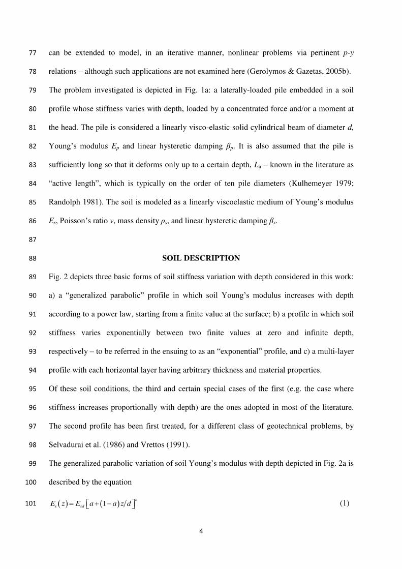
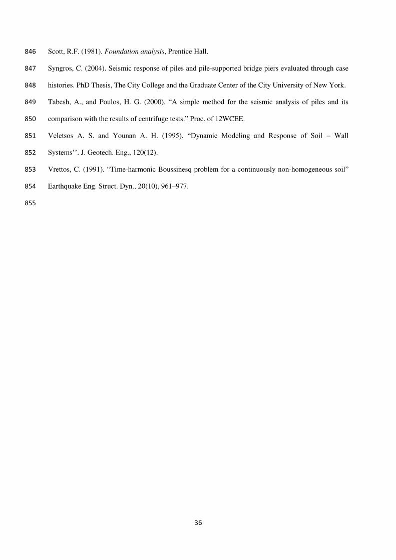
The problem investigated is depicted in Fig. 1a: a laterally-loaded pile embedded in a soil 79
profile whose stiffness varies with depth, loaded by a concentrated force and/or a moment at 80
the head. The pile is considered a linearly visco-elastic solid cylindrical beam of diameter d, 81
Young’s modulus Ep and linear hysteretic damping p. It is also assumed that the pile is 82
sufficiently long so that it deforms only up to a certain depth, La – known in the literature as 83
“active length”, which is typically on the order of ten pile diameters (Kulhemeyer 1979; 84
Randolph 1981). The soil is modeled as a linearly viscoelastic medium of Young’s modulus 85
Es, Poisson’s ratio , mass density ρs, and linear hysteretic damping s. 86
87
SOIL DESCRIPTION 88
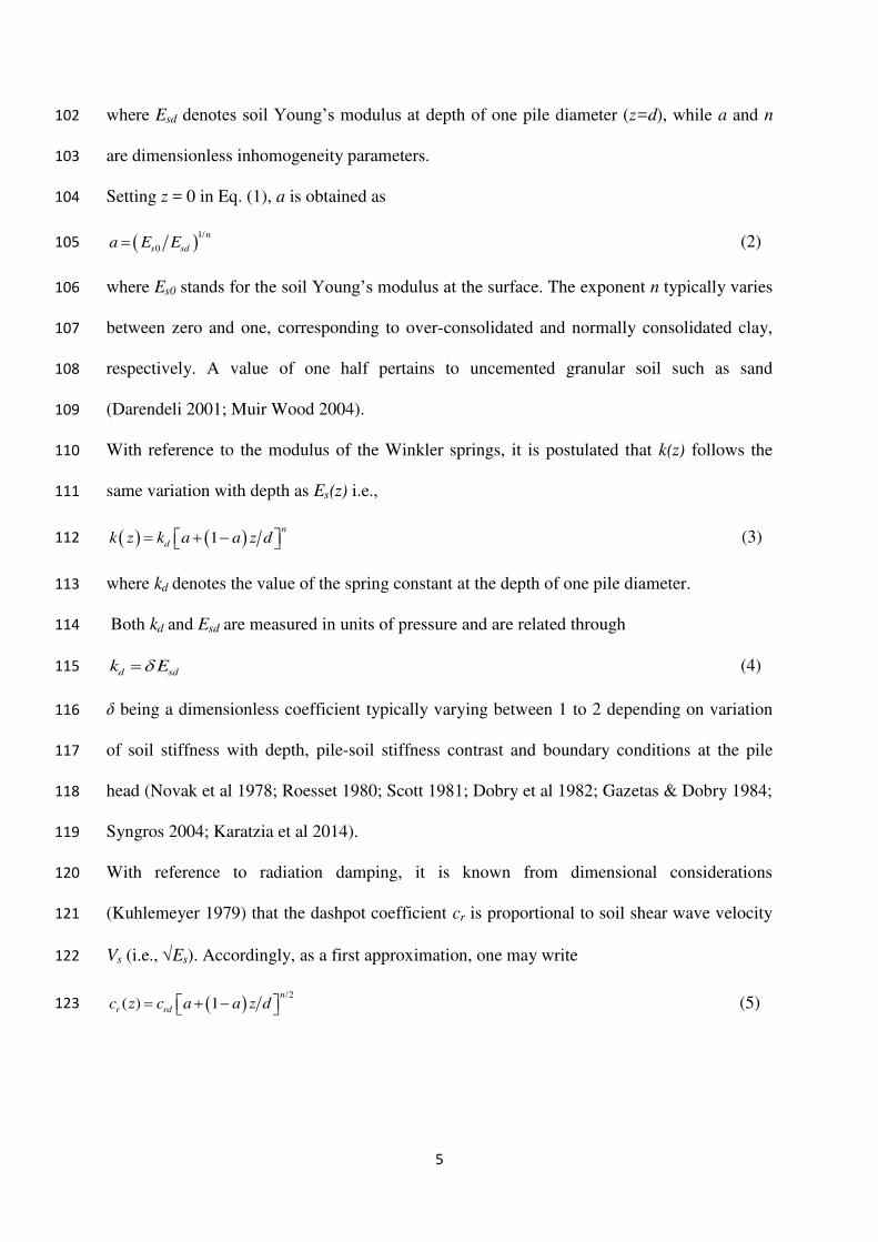
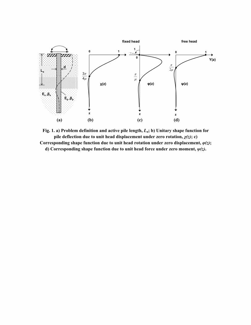
Fig. 2 depicts three basic forms of soil stiffness variation with depth considered in this work: 89
a) a “generalized parabolic” profile in which soil Young’s modulus increases with depth 90
according to a power law, starting from a finite value at the surface; b) a profile in which soil 91
stiffness varies exponentially between two finite values at zero and infinite depth, 92
respectively – to be referred in the ensuing to as an “exponential” profile, and c) a multi-layer 93
profile with each horizontal layer having arbitrary thickness and material properties. 94
Of these soil conditions, the third and certain special cases of the first (e.g. the case where 95
stiffness increases proportionally with depth) are the ones adopted in most of the literature. 96
The second profile has been first treated, for a different class of geotechnical problems, by 97
Selvadurai et al. (1986) and Vrettos (1991). 98
The generalized parabolic variation of soil Young’s modulus with depth depicted in Fig. 2a is 99
described by the equation 100
1n
s sdE z E a a z d (1) 101
5
where Esd denotes soil Young’s modulus at depth of one pile diameter (z=d), while a and n 102
are dimensionless inhomogeneity parameters. 103
Setting z = 0 in Eq. (1), a is obtained as 104
1/
0
n
s sda E E (2) 105
where Es0 stands for the soil Young’s modulus at the surface. The exponent n typically varies 106
between zero and one, corresponding to over-consolidated and normally consolidated clay, 107
respectively. A value of one half pertains to uncemented granular soil such as sand 108
(Darendeli 2001; Muir Wood 2004). 109
With reference to the modulus of the Winkler springs, it is postulated that k(z) follows the 110
same variation with depth as Es(z) i.e., 111
1n
dk z k a a z d (3) 112
where kd denotes the value of the spring constant at the depth of one pile diameter. 113
Both kd and Esd are measured in units of pressure and are related through 114
d sdk E (4) 115
being a dimensionless coefficient typically varying between 1 to 2 depending on variation 116
of soil stiffness with depth, pile-soil stiffness contrast and boundary conditions at the pile 117
head (Novak et al 1978; Roesset 1980; Scott 1981; Dobry et al 1982; Gazetas & Dobry 1984; 118
Syngros 2004; Karatzia et al 2014). 119
With reference to radiation damping, it is known from dimensional considerations 120
(Kuhlemeyer 1979) that the dashpot coefficient cr is proportional to soil shear wave velocity 121
Vs (i.e., Es). Accordingly, as a first approximation, one may write 122
/2
( ) 1n
r rdc z c a a z d (5) 123
6
which reveals a weaker dependence of cr on depth compared to k in Eq. (3). In the above 124
equation crd stands for the dashpot modulus at z = d. Frequency effects on radiation damping 125
are discussed later in this article. 126
Bounded soil inhomogeneity with depth, depicted in Fig. 2b, can be taken into account by 127
considering an exponential variation in Young’s modulus with depth of the form (Vrettos 128
1991) 129
/1 1 q z d
s sE z E b b e (6) 130
in which b stands for the ratio of Young’s moduli at the surface (Es0) and at infinite depth 131
(Es∞), while q is a dimensionless inhomogeneity parameter controlling the rate of increase or 132
decrease in stiffness. 133
In the same vein as in Eqs (3) and (5), the moduli of the Winkler springs and dashpots for the 134
case of bounded soil inhomogeneity can be written as 135
1/2/ /1 1 1 1
,1 1 1 1
q z d q z d
d r rdq q
b b e b b ek z k c z c
b b e b b e
(7a,b) 136
with kd and crd having the same meaning as before. 137
Bounded inhomogeneity such as that expressed by Eqs (6) and (7) might be preferable over 138
the unbounded one in Eqs (1) to (5) for deep soil profiles. However, for shallower profiles 139
either form may be suitable and the selection should be made on a case by case basis. 140
141
RADIATION DAMPING MODEL 142
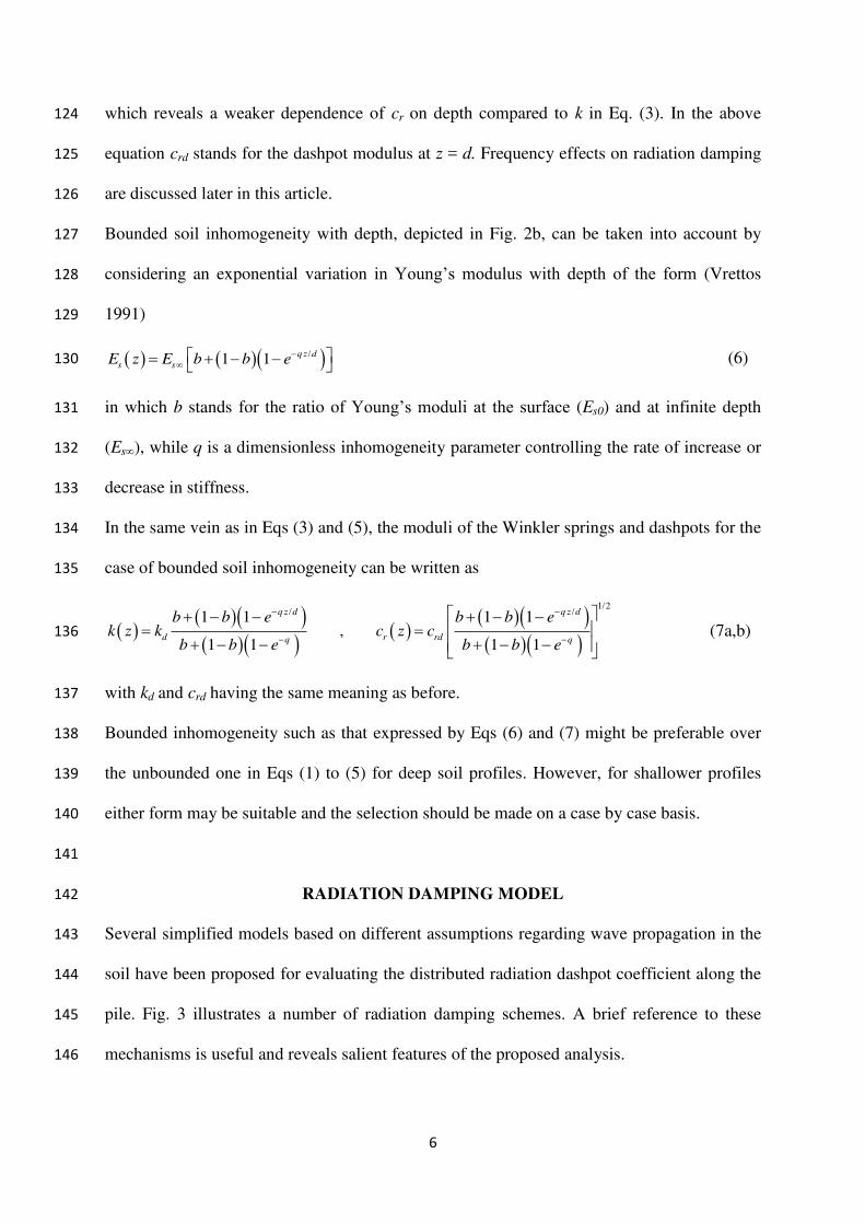
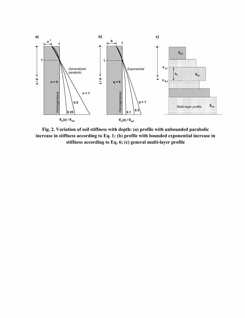
Several simplified models based on different assumptions regarding wave propagation in the 143
soil have been proposed for evaluating the distributed radiation dashpot coefficient along the 144
pile. Fig. 3 illustrates a number of radiation damping schemes. A brief reference to these 145
mechanisms is useful and reveals salient features of the proposed analysis. 146
7
The stripe model of Berger et al (1977) assumes 1D wave propagation in an infinitely long 147
constrained rod and a viscous dashpot which fully absorbs the energy of the emitting waves. 148
Despite its simplicity, this model lacks realism because it provides a strictly frequency-149
independent cr with high sensitivity to Poisson’s ratio, producing an infinite amount of 150
damping as v approaches 0.5. A more rigorous approach has been followed by Novak et al 151
(1978), who proposed a 2D plane-strain model. In this idealization, the soil is divided into an 152
infinite number of thin horizontal “slices”, with each slice subjected to dynamic plane-strain 153
deformation (i.e., z = 0). The resulting radiation damping coefficient is frequency-dependent 154
and decreases monotonically with frequency. The validity of this model has been 155
demonstrated in the works of Blaney et al (1976) and Roesset (1980). 156
An alternative plane-strain scheme has been developed by Gazetas & Dobry (1984). The 157
basic assumption is that the circular cross section of the foundation can be approximated by a 158
square cross section and the surrounding soil is divided into four trapezoidal zones. This 159
formulation allows each of the zones to be analyzed separately as a two-dimensional 160
truncated cone, with compression and extension taking place along the direction of the 161
imposed load and pure shear developing in the perpendicular direction. Based on this 162
formulation, the authors derived an approximate, frequency dependent radiation damping 163
coefficient cr/(dπρsVs) = [1/(2π)]¼[1+(Vs/Vc)
5/4]a0
¼, with a0 ( = d/Vs) being the familiar 164
dimensionless frequency, being the cyclic excitation frequency and Vc standing for the 165
compressional wave propagation velocity in the soil, which was empirically set equal to the 166
so-called Lysmer’s analog wave velocity VLa (= 3.4Vs / [π(1 v)]). 167
An alternative plane-strain model, henceforward referred to as an “infinitesimal sector 168
model”, is illustrated in Fig. 3d. Contrary to the earlier formulation, in the present model the 169
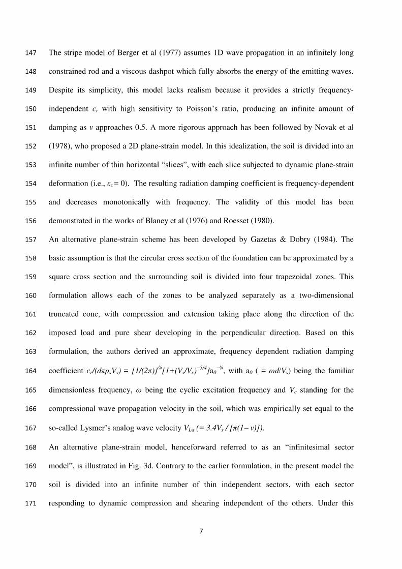
soil is divided into an infinite number of thin independent sectors, with each sector 170
responding to dynamic compression and shearing independent of the others. Under this 171
8
physically-motivated assumption the circular cross section does not need to be replaced by a 172
rectangular one. It is further assumed that each of the independent infinitesimal sectors emits 173
shear and compressional waves, considering that in the loading direction and the 174
perpendicular one propagate only compressional and shear waves, respectively. Shear waves 175
are assumed to propagate with velocity Vs, while compression waves propagate with velocity 176
Vc. As shown in the Supplemental Data File, each sector possesses an infinitesimal amount of 177
stiffness expressed in the global reference system as a function of the polar angle defined in 178
Fig. 3d and the dimensionless frequency a0. 179
By integrating the contributions of all sectors, it is easy to show that the spring and the 180
radiation damping coefficient in an undamped soil medium are, respectively 181
0
1 1a Re , Im
2 2
r
s s s
ck
G d V
(8a,b) 182
where, 183
(2) (2)1 1 0 1 0
(2)(2)0 00 0
1 1a a
2 2
11aa
22
s
cs
c s
c
VH H
VV
V VHH
V
(9) 184
is a dimensionless function of frequency, H0(2)
and H1(2)
being, respectively, the zero- and 185
first-order Hankel functions of the second kind. 186
The relationship in Eqs (8b) and (9) is identical to that of Gazetas & Dobry (1984), except for 187
the generic velocity ratio (Vs/Vc) – instead of an empirically defined compression velocity of 188
the earlier model – and the absence of a multiplier π/4, which reflects the ratio of the side 189
length to the diameter of a square pile cross section and a circular one, respectively, of equal 190
perimeters. Evidently, these differences do not affect the functional form of the solution, yet 191
may have an appreciable impact on the numerical results, as demonstrated in the following. 192
It should be noticed that contrary to the aforementioned models, the horizontal soil slices are 193
considered here to be semi-restricted (i.e., it is assumed that the vertical dynamic stress 194
9
increment σz is zero, instead of the corresponding shear strain z), a superior approximation 195
accounting for the effect of the free surface and leading to solutions not strongly dependent 196
on Poisson’s ratio, in agreement with rigorous numerical solutions of related problems 197
(Veletsos & Younan 1995; Anoyatis & Mylonakis 2012). In light of this assumption, Vs/Vc = 198
[(1 v)/2]1/2
. A detailed discussion of this equation is provided in Anoyatis et al (2016). 199
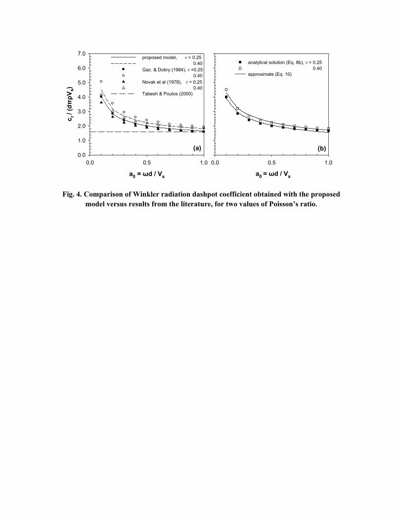
A comparison of the predictions of the proposed model against those available in the 200
literature is provided in Fig. 4a for the cases where v = 0.25 and 0.4. Evidently, there is good 201
agreement between the four solutions. The Tabesh & Poulos (2000) proposal of cr = 5dpsVs 202
seems to provide a reasonable approximation for dimensionless frequencies a0 on the order of 203
1. At higher frequencies it can be shown that Λ approaches asymptotically the purely 204
imaginary value i[1+(Vs/Vc)−1
] and, thereby, the radiation dashpot cr becomes frequency 205
independent while the spring constant vanishes, as in the one dimensional case. 206
Using non-linear regression analysis by means of the Levenberg-Marquardt method 207
(Bevington and Robinson 1992) in the results of Fig. 4b in the frequency range 0.1 < a0 < 1, 208
the following predictive equation is derived 209
1
0.4
00.25 0.8 asr
s s c
Vc
d V V
(10) 210
which can be used in applications. It must be noted that the infinitesimal sector model also 211
provides information on Winkler spring stiffness (Eq. 8a). However, the stiffness tends to 212
zero both at low and high frequencies and, thereby, the solution is of limited value. An 213
enhanced stiffness model is presented later in this article. 214
215
PILE STIFFNESS MODEL 216
Under harmonic oscillations, the equation of motion of a uniform pile attached to a Winkler 217
foundation with variable modulus k(z) and cr(z), is (Mylonakis 1995) 218
10
4
2
40p p r
d YE I k z m i c z
d zY (11) 219
where Y = Y(z) exp[i t] is the harmonic pile deflection as a function of depth z; EpIp is the 220
pile flexural stiffness, m is the pile mass per unit length, k(z) and cr(z) are the moduli of 221
Winkler springs and dashpots, being the cyclic excitation frequency and i = √ –1. 222
In case of a homogeneous soil layer, solving Eq. (11) is straightforward. The associated 223
impedance coefficients in swaying, rocking and cross swaying-rocking are, respectively 224
(Scott 1981; Dobry et al 1982; Pender 1993; Mylonakis 1995) 225
3 24 , 2 , 2hh p p r r p p hr p pK E I K E I K E I (12a-c) 226
where 227
1/42
4
r
p p
k i c m
E I
(13) 228
is a Winkler parameter, measured in units of 1/Length, which can be interpreted as a 229
wavenumber controlling the attenuation of pile deflection with depth. 230
The basis of the proposed solution is that the unknown deflection function Y(z) in Eq. (11) 231
can be effectively represented by a pair of approximate, twice differentiable, dimensionless 232
unitary functions (z) and φ(z) (Fig. 1). Of these functions, (z) represents the normalized 233
deflected shape of the pile due to a unit head displacement under zero rotation (Fig. 1b), 234
whereas φ(z) is the corresponding deflected shape due to a unit head rotation under zero 235
displacement (Fig. 1c). For long piles, (z) and φ(z) can be well approximated by the 236
deflected shape of a long pile in homogeneous soil (Karatzia & Mylonakis 2012): 237
sin cos , sinz
z ez e z z z z
(14a,b) 238
For a free-head pile loaded by a horizontal head force, the corresponding function is (Fig. 1d) 239
coszz e z (14c) 240
11
In the above equations is a shape parameter analogous to the wavenumber in Eq. (13). In 241
homogeneous soil and coincide. In non-homogeneous soil can be taken as the mean 242
value of within the active length, La, of the pile i.e., 243
a
0a
1,
L
z dzL
(15) 244
It should be noticed that La is defined as the length beyond which the pile behaves as a semi-245
infinite beam that is, an increase in pile length would lead to an asymptotic change (increase 246
or decrease) in lateral stiffness at the pile head, regardless of boundary conditions at the tip. 247
Pertinent expressions for La in various soil profiles are derived in the following. 248
Replacing Y(z) in Eq. (11) with Yo i(z), Yo being the amplitude of motion at the pile head, 249
multiplying by Yo j(z), i, j being any of the shape functions in Eqs (14a) and (14b), and 250
integrating over the length of the pile, it can be easily shown (Mylonakis & Roumbas 2001; 251
Karatzia & Mylonakis 2012) that the stiffness and damping coefficients atop the pile can be 252
determined from the virtual-work equations 253
2
0 0 0
L L L
i j p p i j i j i jK E I z z dz k z z z dz m z z dz (16a) 254
0 0 0
2 2L L Lp p p si j i j i j r i j
E IC z z dz k z z z dz c z z z dz
(16b) 255
which are analogous to energy approximations used in finite-element procedures (Clough & 256
Penzien 1975; Mylonakis 1995). Note that the first two terms in the right-hand side of Eq. 257
(16a) stand for the contribution to the overall stiffness of pile flexural stiffness and soil 258
stiffness, respectively. The contribution of pile inertia to stiffness (third term in Eq. 16a) is 259
typically minor and, thereby, is omitted in the remainder of this work. Accordingly, pile head 260
stiffness can be well approximated by its static value in the frequency range of interest in 261
earthquake engineering applications (Kaynia & Kausel 1982). 262
In Eq. (16b), the first two terms stand for the contributions to overall damping of the pile and 263
the soil material damping, respectively, while the last term corresponds to the contribution of 264
12
soil radiation damping. The method was first employed in the analysis of pile foundations by 265
Dobry et al (1982) and later by Gazetas & Dobry (1984), who determined the swaying 266
damping coefficient Chh using Eq. (16b) in conjunction with a numerically-evaluated shape 267
function for a fixed-head pile. 268
The subscripts i and j in the above formulation refer to different vibrational modes (i.e., 269
swaying and rocking). For instance, using i(z) = j(z) = (z) the swaying impedance 270
coefficients Khh and Chh are obtained. Similarly, setting i(z) = j(z) = φ(z), Eqs (16a,b) yield 271
the rocking impedance coefficients Krr and Crr. Finally, using i(z) = (z) and j(z) = φ(z) 272
generates the cross swaying-rocking impedances Khr and Chr. It is implicitly assumed that (z) 273
and φ(z) are real-valued, obtained by static considerations. Also, for L >La the analysis can be 274
simplified by considering the pile as infinitely long, thereby increasing the upper integration 275
limit in Eqs. (16a,b) to infinity. These approximations have been established in earlier studies 276
by Dobry et al (1982), Mylonakis (1995) and Mylonakis & Gazetas (1999). 277
To develop insight into the physics of the solution, it is useful to adopt a representation of 278
pile head stiffness in the form 279
1p
ij ij ijK K S (17) 280
where Kp
ij denotes the contribution to the overall head stiffness of pile flexural stiffness (first 281
integral in Eq. 16a) and Sij is a dimensionless coefficient which stands for the contribution of 282
the restraining action of soil (second integral in Eq. 16a normalized by the first). 283
Accordingly, 284
3 231 , 1 , 1
2hh p p hh rr p p rr hr p p hrK E I S K E I S K E I S (18a-c) 285
which correspond to the swaying, rocking and cross-swaying-rocking mode, respectively. For 286
homogeneous soil the coefficients Sij equal 3, 1/3 and 1, respectively, according to Eq. (12). 287
In addition, using the normalized damping coefficient at the pile head 288
13
2
ij
ij
ij
C
K
(19) 289
Eq. (16b) yields the dimensionless expression 290
1p p r
ij ij p ij s ij rdw w w (20) 291
where wp
ij, wrij are dimensionless coefficients which stand for the contribution to the overall 292
damping of pile material damping and radiation damping, respectively. These coefficients are 293
dependent on the response mode, type of soil inhomogeneity and Ep/Esd ratio. 294
The distributed radiation damping coefficient along the pile, rd, is 295
2
rdrd
d
c
k
(21) 296
crd being the value of the radiation dashpot at z = d. 297
In the realm of the proposed elastodynamic model, rd = π Im[Λ] a0d / [8(1+v) ] (following 298
Eqs. 4, 8b), a0d being the dimensionless frequency at depth z = d (i.e., d / Vsd). 299
By matching Eqs. (20) and (16b), the weight factors wp
ij are related to Sij in Eq. (17) through 300
1
1
p
ij
ij
wS
(22) 301
which suggests that the dimensionless coefficients Sij and wrij (six factors in total) suffice to 302
describe the dynamic impedance of a cylindrical pile in planar oscillations. 303
304
WINKLER SPRING STIFFNESS MODEL 305
Key to the implementation of the proposed method is the appropriate selection of the Winkler 306
spring coefficient in Eq. (4). This can be done based on a three-dimensional elasticity 307
model for the response of a horizontal soil slice proposed by the senior author (Mylonakis 308
2001). The difference with the slice model in Fig. 3d lies in the horizontal inter-slice shear 309
tractions at the upper and lower faces of the slice which are accounted for, providing finite 310
14
stiffness at all frequencies. The above solution (which contains some clerical errors in the 311
original publication), is further explained in Karatzia et al (2014, 2015) and can be cast as 312
22 1
1 22ln 4 1
1
uuu c ua
v
(23) 313
where u=[(2v)/(1v)]½ is a compressibility coefficient, (= 0.577) is Euler’s number, and 314
αc is a dimensionless parameter accounting for the variation of pile displacement with depth 315
1/22 2
0 0c s sd G z Y z dz G z Y z dz
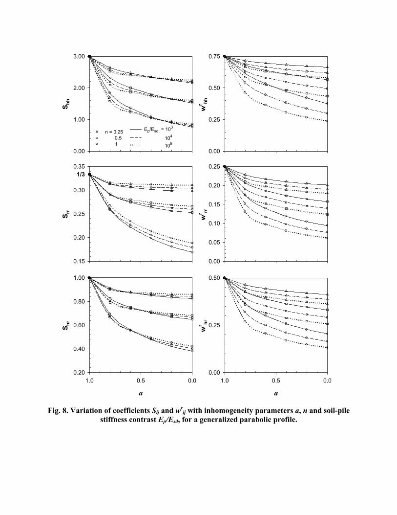
(24) 316
where Y = Y(z) is the deflected shape of the pile in Eq. (11) (Eqs 14a-c for various response 317
modes) and Gs(z) [ = Es(z) / 2(1+ )] is the depth-varying soil shear modulus. 318
Evaluating Eq. (24) yields 319
c p sd
nE E
(25) 320
with and n given in Table 1 for different soil profiles and pile head constraints. It is worth 321
noting that in a shallow soil layer over a rigid base, parameter αc can be interpreted as a 322
cutoff frequency beyond which propagating waves suddenly emerge in the soil. However, for 323
the more general conditions at hand, c can be viewed as a stiffness parameter. 324
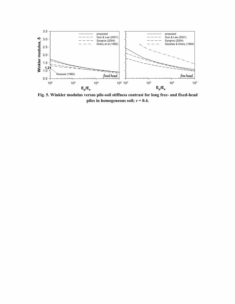
A comparison of the predictions of Eq. (23) against available formulas for parameter is 325
performed graphically in Fig. 5, with reference to fixed- and free-head piles in homogeneous 326
soil. Evidently, the effect of pile head restraint is significant and becomes more pronounced 327
at low pile-soil stiffness contrasts. The proposed model captures satisfactorily this effect. In 328
general, parameter is on the order of 1 and 2 for both fixed- and free-head piles, and tends 329
to decrease with increasing Ep/Es. The proposed analytical solution is in good agreement with 330
the available formulae, especially for stiff piles having Ep/Es ratios greater than 103 or so. 331
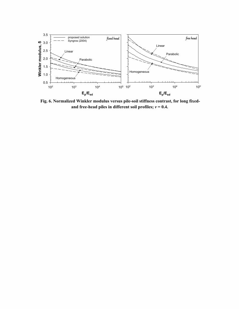
Fig. 6 presents results for parameter in different soil profiles obtained with the proposed 332
model. Clearly, is sensitive to the type of soil profile attaining greater values in soil whose 333
stiffness varies with depth. This is hardly surprising as the gradient of Young’s modulus with 334
15
depth increases the interaction (“arching”) among soil slices at different elevations. With 335
reference to the fixity condition at the pile head, parameter is much higher for free-head 336
piles in the whole range of Ep/Esd values. A comparison of the present solution against results 337
from the finite-element-based solution of Syngros (2004) is presented in the same graph. The 338
accord between the proposed method and the numerical solution cannot be overstated 339
especially for piles with Ep/Esd ratios greater than 103 or so. 340
341
ACTIVE PILE LENGTH 342
It is well-known that the response of a laterally-loaded pile becomes essentially independent 343
of pile length after a critical limit known as “active length”, La. Several empirical formulae 344
have been proposed to estimate this parameter (Kuhlmeyer 1979; Poulos & Davis, 1980; 345
Randolph 1981; Fleming et al 1993; Gazetas 1991; Budhu & Davies 1987; Mylonakis 1995; 346
Syngros 2004; Guo 2012; Di Laora & Rovithis 2015). These are typically written in the form 347
a
Ln
L p sdL d E E (26) 348
L and nL being dimensionless constants; nL is of the order of 0.25 while L lies in the range 349
1.5 to 2.5 depending mainly on type of soil profile and fixity conditions at pile head. 350
In the realm of the present model, a rational estimation of active pile length is possible by 351
means of simple calculations. The investigation at hand focuses on both homogeneous and 352
inhomogeneous soil. Based on Eq. (16a) and the developments of the previous sections, the 353
following dimensionless equation is derived for the stiffness coefficient Khh 354
a a
2 2
23
0
p pL L
tol
p p
E I z dz k z z dz
E I k z z dz
(27) 355
in which (z) is the shape function in Eq. (14a) and tol stands for a tolerance parameter. In the 356
above ratio, the denominator represents the stiffness coefficient Khh of an infinitely long pile 357
whereas the numerator stands for the contribution of the portion of the pile below the active 358
16
length. Accordingly, a value of tol equal to 102
suggests that 99% of the swaying stiffness 359
Khh is contributed by the portion of the pile above La. Based on existing literature (Randolph 360
1981; Syngros 2004), tol is usually taken in the range 102
to 103
. Note that the formulation 361
in Eq. (27) is general and can be applied to both homogeneous and inhomogeneous soil, as 362
well as to different response modes. 363
By applying Eq. (27) to the soil profiles in Fig. 2 and using non-linear regression analysis of 364
the Levenberg-Marquardt type over the range 102 < Ep/Esd < 10
4, the following relationship 365
for the dimensionless parameters of the active pile length was obtained 366
1 2 logL tol (28) 367
parameters 1, 2 and nL are given in Table 2. The analysis reveals that the differences in the 368
value of parameter L in the literature could be attributed to the different tolerance limits 369
adopted in different studies (Fig. 7). 370
It is worth mentioning that using the stiffness terms Krr or Khr instead of Khh in Eq. (27), one 371
obtains approximately the same results for La/d (not shown), which suggests that the effect of 372
the response mode on active pile length is of minor importance. 373
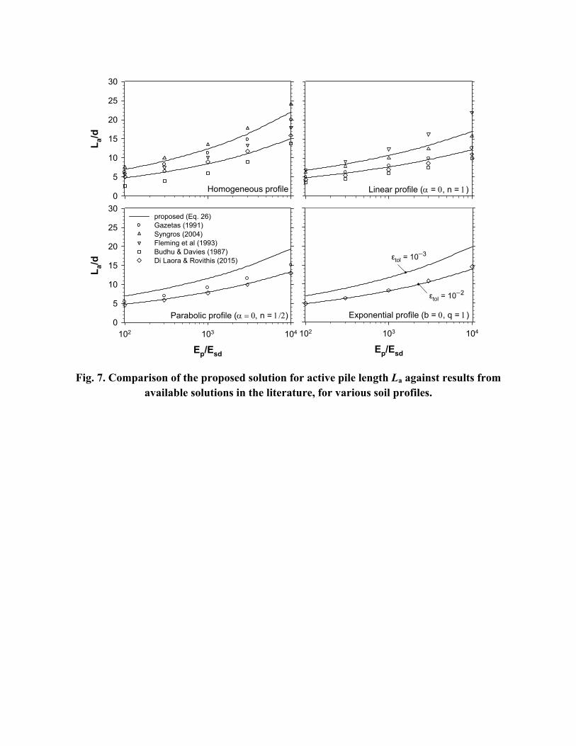
Results for active pile length in various soil profiles obtained by means of Eq. (26) and Table 374
2 are illustrated in Fig. 7, plotted as a function of pile-soil stiffness contrast and different 375
values of the tolerance parameter tol. In the same plot, available solutions from the literature 376
are shown for comparison. Evidently, La/d tends to increase with increasing Ep/Esd and 377
decrease with increasing tol. The sensitivity of La in tol leads to a difference of three to four 378
diameters for Ep/Esd = 103. The proposed solution is in meaningful agreement with those in 379
the literature. An alternative interpretation of active pile length based on the value of 380
dimensionless product ( L) is provided in Di Laora and Rovithis (2015). 381
382
383
17
STIFFNESS AND DAMPING COEFFICIENTS 384
Multi-layer profile 385
For a soil profile consisting of N homogeneous layers up to the active length, the integrals in 386
Eqs. (16a,b) can be evaluated analytically. Expressed in terms of the dimensionless 387
parameters Sij (Eqs. 17, 18), the stiffness coefficients at the pile head are obtained as follows: 388
,
4 2
1 ,
2 cos 2 sin 2
zb iNz
hh i
i zt i
S e z z
(29a) 389
,
4 2
1 ,
12 cos 2 sin 2
3
zb iNz
rr i
i zt i
S e z z
(29b) 390
,
4 2
1 ,
1 sin 2
zb iNz
hr i
i zt i
S e z
(29c) 391
The dimensionless coefficients associated with the radiation damping (rij = C
rij / (2Kij)) 392
are given below 393
,
4 2
1 ,
12 cos 2 sin 2
1
zb iNr zrihh i
hh rdi zt i
w e z zS
(30a) 394
,
4 2
1 ,
1 12 cos 2 sin 2
1 3
zb iNr zrirr i
rr rdi zt i
w e z zS
(30b) 395
,
4 2
1 ,
11 sin 2
1
zb iNr zrihr i
hr rdi zt i
w e zS
(30c) 396
with 397
a
11a
1
i
N L
ih
i
z dzL
(31) 398
in which zt,i denotes the elevation of the upper end of layer i, and zb,i denotes the elevation of 399
the lower end (Fig. 2c); hi is the thickness of the layer, i is the corresponding pile 400
wavenumber and ri (= cri / (2ki)) is the corresponding radiation damping coefficient. Eqs 401
18
(29) and (30) have been presented, in a different form, by Karatzia & Mylonakis (2012). The 402
complementary coefficients wij p can be obtained from Eq. (22). The special case of a bilayer 403
soil profile has been considered by Mylonakis (1995) and Mylonakis & Gazetas (1999). 404
Generalized parabolic profile 405
In case of a soil layer with parabolically varying modulus (a = arbitrary, n = arbitraryEq. 1), 406
the corresponding coefficients are 407
3 14
2 210 11 114
1 142 2 cos sin
4 4
n n
n adhh
n nS e Q a B a
(32a) 408
5 14
2 210 11 114
1 182 2 cos sin
3 4 4
n n
n adr r
n nS e B a Q a
(32b) 409
44
2 210 11 114
42 2 cos sin
4 4
n n
n adhr
n nS e Q a B a
(32c) 410
1 1 16 24
1 14 2 420 21 214
2 242 2 cos sin
8 81
n n n
r adhh
hh
n nw e Q a B a
S
(33a) 411
1 1 110 24
1 14 2 420 21 214
2 282 2 cos sin
8 83 1
n n n
r adr r
r r
n nw e B a Q a
S
412
1 1 184
1 14 2 420 21 214
42 2 cos sin
8 81
n n n
r adhr
hr
n nw e Q a B a
S
(33b,c) 413
where = βd /(1−a) and Γ10, Γ20, Q11, Q21, B11, B21 are dimensionless parameters provided in 414
the Appendix. n1 = (1 ) n, being 0 for frequency independent radiation damping as in 415
Berger et al (1977) and Tabesh and Poulos (2000), and (0.4) for the power law dependence 416
of a00.4
in Eq. 10. d is obtained from Eq. (13) and the corresponding shape parameter is 417
given by 418
4
1 44
a a44
14 1
nn
d L La a a
n a d d
(34) 419
19
The special cases of a soil profile whose Young’s modulus increases linearly with depth (n = 420
1) and one having zero modulus at the soil surface (a = 0, n 0) lead to simpler expressions 421
which are provided in the Supplemental Data File. 422
Generalized exponential profile 423
For the variation in Young’s modulus in Eq. (6) (Fig. 2b), the following closed-form 424
expressions for the pile stiffness and damping were obtained 425
2 2 2
4 2 23
1 3 33
4 2 2 2hh
p p
d b q d dkS
E I q d q d d
(35a) 426
3 2 2 2
2 24
2 2 3 7
3 4 2 2 2r r
p p
b d q q d dkS
E I q d q d d
(35b) 427
2 2 2 2
2 24
2 4 3 3
4 2 2 2hr
p p
b d q d q q d dkS
E I q d q d d
(35c) 428
2
4
0 1 2
4
2
1 1 1
dr
hh nq
hh
A J Jw
S b b e
(36a) 429
2
4
0 1 2
4
2
3 1 1 1
dr
r r nq
r r
A J Jw
S b b e
(36b) 430
2
4
0 1 3
4
2
2 1 1 1
dr
hr nq
hr
A J Jw
S b b e
(36c) 431
where dimensionless parameters A0, J1, J2 and J3 are defined in the Appendix. n2 = (1 )/2, 432
having the same meaning as before. 433
Shape parameter is given by 434
a
a1/43/4
1/4
1 21 4
a
4 13 1 1 3
1 13 1 1
qLqL d
d dp p
q
d eb H b e H
b bqL b b e
(37) 435
20
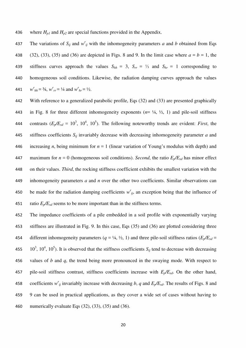
where Hp1 and Hp2 are special functions provided in the Appendix. 436
The variations of Sij and wrij with the inhomogeneity parameters a and b obtained from Eqs 437
(32), (33), (35) and (36) are depicted in Figs. 8 and 9. In the limit case where a = b = 1, the 438
stiffness curves approach the values Shh = 3, Srr = ⅓ and Shr = 1 corresponding to 439
homogeneous soil conditions. Likewise, the radiation damping curves approach the values 440
wrhh = ¾, w
rrr = ¼ and w
rhr = ½. 441
With reference to a generalized parabolic profile, Eqs (32) and (33) are presented graphically 442
in Fig. 8 for three different inhomogeneity exponents (n= ¼, ½, 1) and pile-soil stiffness 443
contrasts (Ep/Esd = 103, 10
4, 10
5). The following noteworthy trends are evident: First, the 444
stiffness coefficients Sij invariably decrease with decreasing inhomogeneity parameter a and 445
increasing n, being minimum for n = 1 (linear variation of Young’s modulus with depth) and 446
maximum for n = 0 (homogeneous soil conditions). Second, the ratio Ep/Esd has minor effect 447
on their values. Third, the rocking stiffness coefficient exhibits the smallest variation with the 448
inhomogeneity parameters a and n over the other two coefficients. Similar observations can 449
be made for the radiation damping coefficients wrij, an exception being that the influence of 450
ratio Ep/Esd seems to be more important than in the stiffness terms. 451
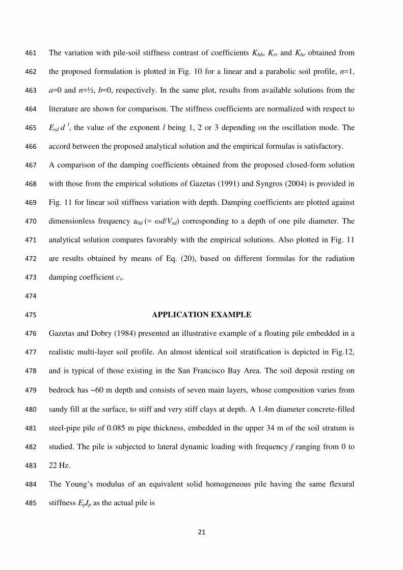
The impedance coefficients of a pile embedded in a soil profile with exponentially varying 452
stiffness are illustrated in Fig. 9. In this case, Eqs (35) and (36) are plotted considering three 453
different inhomogeneity parameters (q = ¼, ½, 1) and three pile-soil stiffness ratios (Ep/Esd = 454
103, 10
4, 10
5). It is observed that the stiffness coefficients Sij tend to decrease with decreasing 455
values of b and q, the trend being more pronounced in the swaying mode. With respect to 456
pile-soil stiffness contrast, stiffness coefficients increase with Ep/Esd. On the other hand, 457
coefficients wrij invariably increase with decreasing b, q and Ep/Esd. The results of Figs. 8 and 458
9 can be used in practical applications, as they cover a wide set of cases without having to 459
numerically evaluate Eqs (32), (33), (35) and (36). 460
21
The variation with pile-soil stiffness contrast of coefficients Khh, Krr and Khr obtained from 461
the proposed formulation is plotted in Fig. 10 for a linear and a parabolic soil profile, n=1, 462
a=0 and n=½, b=0, respectively. In the same plot, results from available solutions from the 463
literature are shown for comparison. The stiffness coefficients are normalized with respect to 464
Esd d l, the value of the exponent l being 1, 2 or 3 depending on the oscillation mode. The 465
accord between the proposed analytical solution and the empirical formulas is satisfactory. 466
A comparison of the damping coefficients obtained from the proposed closed-form solution 467
with those from the empirical solutions of Gazetas (1991) and Syngros (2004) is provided in 468
Fig. 11 for linear soil stiffness variation with depth. Damping coefficients are plotted against 469
dimensionless frequency a0d (= d/Vsd) corresponding to a depth of one pile diameter. The 470
analytical solution compares favorably with the empirical solutions. Also plotted in Fig. 11 471
are results obtained by means of Eq. (20), based on different formulas for the radiation 472
damping coefficient cr. 473
474
APPLICATION EXAMPLE 475
Gazetas and Dobry (1984) presented an illustrative example of a floating pile embedded in a 476
realistic multi-layer soil profile. An almost identical soil stratification is depicted in Fig.12, 477
and is typical of those existing in the San Francisco Bay Area. The soil deposit resting on 478
bedrock has 60 m depth and consists of seven main layers, whose composition varies from 479
sandy fill at the surface, to stiff and very stiff clays at depth. A 1.4m diameter concrete-filled 480
steel-pipe pile of 0.085 m pipe thickness, embedded in the upper 34 m of the soil stratum is 481
studied. The pile is subjected to lateral dynamic loading with frequency f ranging from 0 to 482
22 Hz. 483
The Young’s modulus of an equivalent solid homogeneous pile having the same flexural 484
stiffness EpIp as the actual pile is 485
22
4 4 78 8
8
2 2 0.085 2.5 101 1 1 2.5 10 1 1 1 1.15 10 a
1.4 2.5 10
w cp st
st
t EE E kP
d E
(38) 486
Step 1: The active pile length should be determined considering the soil inhomogeneity. As a 487
first approximation, the solution corresponding to linear inhomogeneity with depth (n = 1) 488
will be utilized. Thus, La is computed by means of Eq. (26) selecting the parameters for a 489
linear profile (Table 2), with tolerance tol = 102, Ep/Esd = 1.1510
8/1.3210
5 = 870, to get 490
the estimate La = 10.4m (7d). This suggests that the first two layers, the thick sandy fill and 491
the normally consolidated San Francisco Bay Mud, mainly contribute to the lateral response 492
of pile. Therefore, the stiffness and damping coefficients are obtained using Eqs (29)-(30) 493
considering the contribution of the upper two soil layers, with each layer having constant 494
Young’s modulus, i.e., Es1 = 132 MPa and Es2 = 86 MPa, respectively. Accordingly, the pile-495
soil stiffness ratio Ep/Esd required for computing La is 870. Remarkably, the resulting active 496
length is half of that predicted in the original example based on dynamic considerations. 497
Step 2: The Winkler constant for each layer is obtained by means of Eqs (23) and (25) 498
selecting the parameters for homogeneous profile (Table 1), to get =1.35 as an average 499
value in the first two layers. 500
Step 3: The Winkler parameters corresponding to the surface upper and the underlying layer 501
are obtained by applying Eq (13), to be found 1 = 0.213 m1 and 2 = 0.191 m1
, respectively. 502
Accordingly, the shape parameter (Eq 31) attains the anticipated average value 503
114.2 0.213 10.4 4.2 0.191 0.2
10.4m (39) 504
Step 4: The stiffness coefficients Sij are computed by evaluating Eqs (29a-c) as follows 505
44.2
2 0.2
0
410.4
2 0.2
4.2
0.2132 cos 2 0.2 sin 2 0.2
0.2
0.1912 cos 2 0.2 sin 2 0.2 3.61
0.2
zhh
z
S e z z
e z z
(40a) 506
23
4 4.22 0.2
0
4 10.42 0.2
4.2
0.213 12 cos 2 0.2 sin 2 0.2
0.2 3
0.191 12 cos 2 0.2 sin 2 0.2 0.33
0.2 3
zrr
z
S e z z
e z z
(40b) 507
44.2
2 0.2
0
410.4
2 0.2
4.2
0.2131 sin 2 0.2
0.2
0.1911 sin 2 0.2 1.12
0.2
zhr
z
S e z
e z
(40c) 508
where the subscripts and superscripts following the curly braces denote difference between 509
values at two elevations. 510
Step 5: By substituting the predicted stiffness coefficients Sij to Eqs (18a-c) yields the 511
stiffness values Khh = 0.8106 kN/m, Krr = 8.710
6 kNm and Khr = 1.810
6 kN. Khh deviates 512
by a mere 10% from the finite-element result reported by Gazetas and Dobry (1984). 513
Step 6: It is straightforward to obtain the dimensionless weight factors w pij via Eq. (22), i.e., 514
w phh = 0.22, w
prr = 0.75, w
phr = 0.47. 515
Step 7: As for the radiation damping coefficient r, Eqs. (10) and (21) are utilized, keeping in 516
mind that the properties are constant within each layer. In the first layer, using Vs/Vc = 0.61 517
corresponding to v = 0.25, Eq. (10) yields 518
cr1 = 1.4π1.85169(0.25 + 0.80.611
)(2 π f1.4/169)0.4 7000 f
0.4 (kPas) (41a) 519
For the second layer, using Vs/Vc = 0.5, Eq. (10) provides 520
cr2 = 1.4π1.7130(0.25 + 0.80.51
)(2 π f1.4/130)0.4 5300 f
0.4 (kPas) (41b) 521
Since k1=1.351.32105=1.810
5 kPa and k2=1.350.8610
5=1.210
5 kPa, Eq.(21) yields 522
0.4 0.6 0.4 0.6
1 25 5
2 27000 0.122 , 5300 0.139
2 1.8 10 2 1.2 10r r
f ff f f f
(42a,b) 523
Step 8: In the same vein and using rd = r1, damping coefficients wrij (Eq. 30) are estimated 524
as wrhh = 0.79, w
rhr = 0.55, w
rrr = 0.27. 525
Step 9: Applying Eq. (20) leads to the following expressions 526
24
hh = 0.220.02+(10.22)0.04+0.790.122 f 0.6
= 0.036+0.096 f 0.6
(43a) 527
hr = 0.470.02+(10.47)0.04+0.550.122 f 0.6
= 0.031+0.067 f 0.6
(43b) 528
rr = 0.750.02+(10.75)0.04+0.270.122 f 0.6
= 0.025+0.033 f 0.6
(43c) 529
For simplicity, a fixed value s = 0.04 is adopted for the soil material damping pertaining to 530
the sand material in the upper soil layer. The damping coefficients are illustrated in Fig.13. 531
Alternative Solution for Linear Profile 532
The same problem may be solved by replacing the actual multi-layer soil profile with an 533
equivalent idealized linear profile. Although this is not essential in the present case (where 534
adequate information for the subsoil is available) the example is solved on the basis of this 535
assumption to demonstrate the applicability of the proposed method and facilitate 536
understanding of the various steps. 537
Without loss of accuracy, the variation of Young’s modulus within the actual soil deposit can 538
be described by the linear function of depth obtained using linear regression, (Fig.12), 539
Es(z) = 85.6 (0.85 + 0.11z) MPa (44) 540
Note that performing the regression within a shallower range, say within the upper one third 541
of the pile, corresponding to the active length, does not significantly alter the results. To 542
determine the impedance at the pile head, one may utilize the expressions for stiffness and 543
damping coefficients pertaining to the generalized parabolic profile (a0, n0). 544
Step 1: According to the proposed method, the inhomogeneity parameters a and n, and the 545
reference Young’s modulus at depth of one pile diameter are first evaluated at Esd = 85.6 546
MPa, a = Es0/Esd 0.85, n = 1, resulting from matching Eqs (1) and (44). 547
Step 2: Having determined the ratio Ep/Esd = 1.15108/0.85610
5 = 1.3410
3, La is given by 548
Eq. (26) and Table 2, considering the same parameters as before (assuming tolerance tol = 549
102), to get La =11m (8d). 550
25
Step 3: From Eqs (23) and (25) and choosing the values = 1.633 and n = 0.2 from Table 551
1, pertaining to linear soil stiffness variation with depth, fixed head piles and v = 0.4, 552
parameter is estimated at 1.74. 553
Step 4: Using a = 0.85, n = 1 and d = 0.2 m1
, the shape parameter obtained from Eq (34) 554
is obtained at 0.22 m1
. 555
Step 5: Stiffness coefficients are given by Eqs (32a-c). Parameter is found to be 4.15, while 556
via Eq. 52b and setting n*= n = 1, parameters Γ10, Γ11, B11 and Q11 are estimated to be 557
Γ10 = (4.150.85)e4.150.85
[1+1/(4.150.85)] = 0.13 (45a) 558
Γ11 = [4.150.85(1+ i)]e4.150.85(1+ i)
{1+1/[4.150.85(1+ i)]}= 0.162 0.045i (45b) 559
B11 = Re[Γ11] = 0.162, Q11 = Im[Γ11] = 0.045 (45c,d) 560
The application of Eqs (32a-c) using the above values yields 561
42 1 4.15 0.85
4
4 0.22 4.15
0.22
2 0.13 0.045 cos 2 4.15 0.85 0.162 sin 2 4.15 0.85 2.3
hhS e
(46a) 562
43 1 4.15 0.85
4
8 0.22 4.15
3 0.22
2 0.13 0.162 cos 2 4.15 0.85 0.045 sin 2 4.15 0.85 0.31
rrS e
(46b) 563
541 4.15 0.852
4
1 2
4 0.22 4.15
0.22
2 0.13 0.045 cos 4 4.15 0.85 0.162 sin 4 4.15 0.85 0.85
hrS e
(46c) 564
which suggest that soil contributes 2.3, 0.31 and 0.85 times the amount of stiffness provided 565
by the pile element in swaying, rocking and cross swaying-rocking, respectively. 566
Step 6: Eqs (18a-c) provide the stiffness values Khh = 0.79106 kN/m, Krr = 9.510
6 kNm and 567
Khr = 2106 kN. These results are in good agreement with those obtained using the multi-568
layer actual profile with discrepancies of 1%, 8% and 10%, respectively. 569
Using the simpler expressions provided in the Supplemental Data File (Eq. S9) yields 570
26
4
5
3 0.21 0.85 2 1.4 0.22 1 2.24
2 1.4 0.22hhS
(47a) 571
4
5
0.21 0.85 1.4 0.22 1 0.3
3 1.4 0.22rrS
(47b) 572
4
5
0.23 0.85 4 1.4 0.22 3 0.83
4 1.4 0.22hrS
(47c) 573
which practically coincide with results in Eq. (46) (differences being due to cut-off errors). 574
Step 7: Applying an analogous procedure for the coefficients wrij, using n1 = (1 (0.4))1 = 575
1.4, Eqs (33a-c) lead to wrhh = 0.67, w
rrr = 0.21, w
rhr= 0.42. Eq. (22) provides the coefficients 576
w p
ij, associated with the pile material damping, i.e, w p
hh = 0.30, w p
rr = 0.76, w phr = 0.54. 577
Step 8: Subsequently, the dashpot coefficient cr (Eq. 10) computed at depth of one pile 578
diameter according to Eq. (21) is estimated to be 579
crd = 1.4π1.85129(0.25+0.80.51
)(2πf 1.4/129)0.4 5200 f
0.4 (kPas) (48) 580
Step 9: Considering kd = 1.5105 kPa, the radiation damping coefficient is rd = 0.11f
0.6. 581
Step 10: Finally, the expressions for the dimensionless damping coefficients are 582
hh = 0.034+0.074 f 0.6
, hr = 0.029+0.048 f 0.6
, rr = 0.025+0.024 f 0.6
(49a-c) 583
Alternative Solution for an Exponential Profile 584
As a second alternative, an idealized exponential soil profile is employed. 585
Step 1: It is assumed that Es = 480 MPa, thus b = Es0/ Es = 58/480 0.1, and q = 0.1. The 586
stiffness variation with depth z, depicted in Fig.12, is 587
Es(z) = 480 [0.1+0.9 (1 e0.07z
)] MPa (50) 588
Step 2: Considering Ep/Esd= 1.15108/0.8910
5 = 1.310
3, La is obtained by Eq. (26) and 589
Table 2, assuming tol = 102, at La =12m (8.5d). 590
27
Step 3: From Eqs. (23) and (25) and using the values = 1.34 and n = 0.23 from Table 1, 591
for an exponential soil profile and a fixed head pile, parameter is estimated at 1.4 (Poisson’s 592
ratio taken equal to 0.4). 593
Step 4: Using b = q = 0.1, and d = 0.19 m1
, the shape parameter (Eq. 37) is 0.23 m1
. 594
Step 5: From Eqs. (35a-c) with k = 1.44.8105= 6.710
5 kPa, it is straightforward to obtain 595
the stiffness coefficients Shh = 1.84, Srr = 0.30 and Shr = 0.77. 596
Step 6: Evaluating Eqs. (18a-c) yield the stiffnesses Khh = 0.75106 kN/m, Krr = 9.710
6 kNm 597
and Khr = 2106 kN, which are very similar to those obtained above and highlight the 598
insensitivity of the solution to soil stiffness at depth. 599
Step 7: Using again n2 = (1(0.4)) / 2 = 0.7, parameters A0, J1, J2 and J3 are numerically 600
evaluated using standard mathematical software at A0 = 0.34, J1 = 0.066, J2 = 0.288 and J3 = 601
0.066. Substituting the above values into Eqs. (36a-c) yields wrhh = 0.55, w
rrr = 0.18, w
rhr= 602
0.35, while Eq. (22) yields w phh = 0.35, w
prr = 0.77, w
phr = 0.56. 603
Step 8: Evaluating Eq. (10) leads to crd 5300 f 0.4
kPas (similar result with linear profile). 604
Step 9: Considering kd = 1.2105 kPa, the radiation damping coefficient is rd = 0.14f
0.6. 605
Step 10: Finally, the expressions for the dimensionless damping coefficients are 606
hh = 0.033+0.078 f 0.6
, hr = 0.029+0.049 f 0.6
, rr = 0.025+0.025 f 0.6
(51a-c) 607
608
CONCLUSIONS 609
An approximate, practically-oriented analysis procedure was developed for estimating the 610
dynamic stiffness and damping (impedance coefficients) of a laterally-loaded pile in different 611
types of vertically inhomogeneous soil. To this end, a dynamic Winkler model was adopted 612
in conjunction with a virtual-work scheme associated with approximate shape functions for 613
the pile deflection under imposed head displacements and rotations. Two auxiliary models for 614
28
determining the moduli of the distributed Winkler springs and dashpots were also outlined. 615
The main conclusions of the study are: 616
1. The proposed analytical technique allows closed-form solutions for the pile stiffness and 617
damping at the pile head to be obtained for both bounded and unbounded, layered soil and 618
soil whose stiffness varies smoothly with depth. Results are provided in dimensionless 619
form, which sheds light into the physics of the problem, including the relative 620
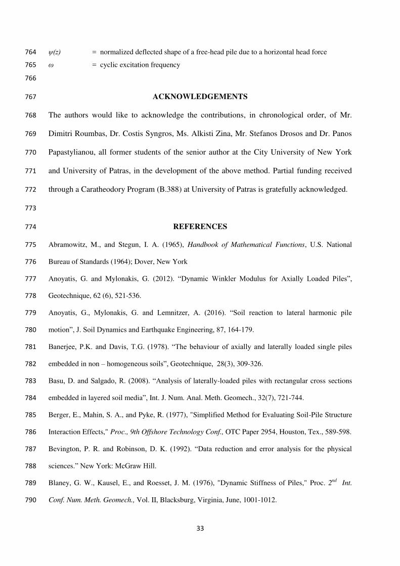
contributions to overall stiffness and damping of the pile and soil components. The insight 621
offered by this modular approach is hardly possible with rigorous numerical solutions such 622
as finite elements. 623
2. Unlike earlier approximate methods, where a limited number of impedance coefficients 624
are determined, this work covers all six impedance coefficients (i.e., Khh, Krr, Khr, Chh, Crr, 625
Chr) in different soil profiles. The method is self-standing and does not involve empirical 626
information. The solutions have been further improved by employing enhanced 627
expressions for various parameters as summarized in the following. 628
3. A new model was developed for the distributed Winkler radiation damping coefficient 629
based on a 2D plane strain infinitesimal sector idealization. It was found that, contrary to 630
trends suggested by existing formulae, the dashpot coefficient does not tend to zero at high 631
frequencies, but approaches asymptotically the value cr = 1.4 d π ρs Vs. On the other hand, 632
the 2D plane strain stiffness k goes to zero both at low and high frequencies. 633
4. A new analytical formulation was developed for the distributed Winkler spring coefficient 634
along the pile, extending an earlier 3D elasticity model by the senior author. In 635
homogeneous soil, Winkler modulus k varies between 12 Es for both fixed- and free-head 636
piles, whereas for inhomogeneous soil, k 12 Esd for fixed-head and 1.53 Esd for free-637
head piles. 638
29
5. A novel solution (Eqs. 26-27, Table 2) was derived for the active pile length in different 639
soil profiles. The associated correlation coefficients encompass a tolerance parameter ( tol) 640
which helps to explain discrepancies in the results reported in the literature. For Ep/Esd 641
values in the range 102 and 10
3, La varies between 5 and 13d. The largest La occurs in 642
homogeneous soil, and the smallest in a linear profile. 643
6. Results for pile stiffness and damping obtained with the proposed method are in good 644
agreement with available numerical solutions and fitted formulae. Coefficients Sij indicate 645
that in the lateral mode soil contributes to the overall stiffness between 1 and 3 times the 646
stiffness provided by the pile. In the other two modes the soil contribution is much 647
smaller, ranging between 0.4 and 1 in cross swaying-rocking and 0.17 to 0.34 in rocking. 648
7. The proposed method can be implemented by means of hand calculations or simple 649
computer spreadsheets and, thereby, can be used in routine calculations for designing piles 650
against lateral dynamic loads. 651
As a final remark, it is noted that nonlinear effects such as those described by p-y curves can 652
be readily incorporated in the solution, via iterative application of the equations of the layered 653
profile until convergence is achieved. Such applications lie beyond the scope of this work. 654
655
APPENDIX: PARAMETERS FOR STIFFNESS & DAMPING COEFFICIENTS 656
In Eqs (32) and (33) parameters Γ10, Γ20, B11 = Re[Γ11], B21 = Re[Γ21], Q11 = Im[Γ11], 657
Q21=Im[Γ21] are obtained from the generalized Gamma function 658
2, 1 , 1,2 , 0,1
1op
n o daip o p
o a
(52a) 659
with n* being n and n1 for stiffness and damping coefficients, respectively. For a = 0, it can 660
be approximated by Stirling’s formula (see Supplemental Data File); for a > 0.5 the following 661
approximation applies (Abramowitz & Stegun 1965) 662
30
1
1 1 , 1,2 , 0,11
na i p
oop
na i p e o p
o a i p
(52b) 663
In Eqs (36a-c) parameters A0, J1=Im[A1], J2=Re[A1] and J3=Im[A1] are denoted as 664
* 2 1 2 , 1 2 ;1 1 2 ;1tA F n i t d q i t d q b (53) 665
with At* being a hypergeometric function in which the subscript t* takes the values −1, 0 and 666
1. 667
In Eq. (37) parameters Hp1 and Hp2 denote the following hypergeometric functions 668
a
1 2 1 2 2 1
3 3 7 1 7, , ; , 1,1, ; 1
4 4 4 1 4
qL
dp pH F H F e b
b
(54a,b) 669
which can be evaluated using standard computer software such as Matlab and Mathematica. 670
671
ΝΟΤΑΤΙΟΝ 672
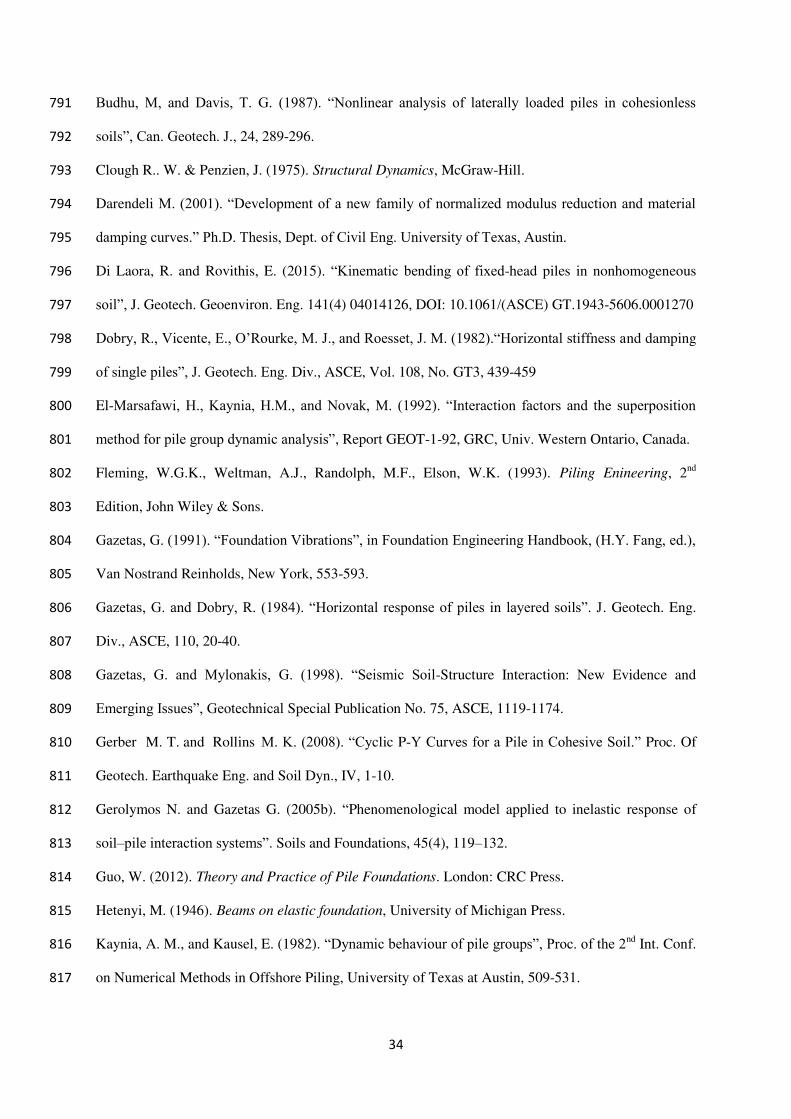
The following symbols are used in this paper: 673
Latin symbols 674
At* = hypergeometric function 675
a0 = dimensionless frequency 676
a0d = dimensionless frequency at depth z = d 677
B11, B21 = real part of generalized Gamma functions Γ11 and Γ21, respectively 678
b = dimensionless inhomogeneity parameter for exponential soil profile 679
Chh, Crr, Chr, Cij = damping coefficients in swaying, rocking and cross swaying-rocking at pile head 680
cr, cr(z) = Winkler radiation dashpot modulus 681
crd = Winkler radiation dashpot modulus at depth of one pile diameter 682
cri = dashpot modulus of soil layer i 683
d = pile diameter 684
Es, Es(z) = soil Young’s modulus 685
Es0, Esd, Es = soil Young’s modulus at soil surface, at depth of one pile diameter, and at infinite 686
depth, respectively 687
Ep = pile Young’s modulus 688
EpIp = pile flexural stiffness 689
Ec, Est = Young’s modulus of concrete and steel pile, respectively 690
p = Young’s modulus of an equivalent solid non hollow pile 691
31
f = excitation frequency 692
Gs, Gs(z) = soil shear modulus 693
H0(2)
, H1(2)
= zero- and first-order Hankel functions of the second kind 694
Hp1, Hp2 = hypergeometric functions 695
hi = thickness of soil layer i 696
i = imaginary unit, number of soil layer in multilayered soil (subscript) 697
ij = refers to different vibrational modes 698
J1, J2 = imaginary and real part of hypergeometric function A1, respectively 699
J3 = imaginary part of hypergeometric function A1 700
k, k(z) = Winkler spring modulus 701
kd, k = Winkler spring modulus at depth z = d and at infinite depth, respectively 702
ki = Winkler spring modulus of soil layer i 703
Khh, Krr, Khr, Kij = pile head stiffness coefficients in swaying, rocking and cross swaying-rocking at 704
pile head 705
Kp
ij = contribution to overall head stiffness of pile flexural stiffness 706
L = pile length 707
La = active pile length 708
l = exponent 1, 2 or 3 depending on oscillation mode 709
m = pile mass per unit length 710
Ν = number of homogeneous layers 711
n = dimensionless inhomogeneity exponent for generalized parabolic soil profile 712
n1, n2, n* = dimensionless parameters 713
n , nL = dimensionless coefficients 714
o, p = arguments of generalized Gamma function 715
q = dimensionless inhomogeneity exponent for exponential soil profile 716
Q11, Q21 = imaginary part of generalized Gamma functions Γ11 and Γ21, respectively 717
Sij = dimensionless stiffness coefficient expressing the contribution of the restraining 718
action of soil to the overall head stiffness 719
t = time 720
tw = wall thickness of hollow pile 721
t* = argument of hypergeometric function 722
Vc = soil compressional wave propagation velocity 723
Vs = soil shear wave propagation velocity 724
Vsd = soil shear wave velocity at depth of one pile diameter 725
VLa = Lysmer’s analog wave propagation velocity 726
wp
ij,wrij = weight factors expressing the contribution of pile material and radiation damping, 727
32
respectively, to the overall damping 728
Yo = amplitude of motion at pile head 729
Y, Y(z) = pile deflection 730
z = depth 731
zt,i, zb,i = elevation of upper (t) and lower (b) face of soil layer i 732
Greek symbols 733
a = dimensionless inhomogeneity parameter for generalized parabolic soil profile 734
ac = dimensionless stiffness parameter 735
p = pile hysteretic damping 736
s = soil hysteretic damping 737
rd = radiation damping coefficient at depth of one pile diameter 738
ij = normalized damping coefficients at pile head 739
ri = dimensionless damping coefficient of soil layer i 740
= Euler’s number ( 0.577) 741
Γop = generalized Gamma function 742
= Winkler spring coefficient 743
tol = tolerance parameter 744
z = vertical normal strain 745
u = compressibility coefficient 746
= dimensionless coefficient 747
, (z) = Winkler wavenumber parameter (1/Length) 748
d = Winkler wavenumber parameter at depth of one pile diameter 749
i, i (z) = Winkler wavenumber parameter of soil layer i 750
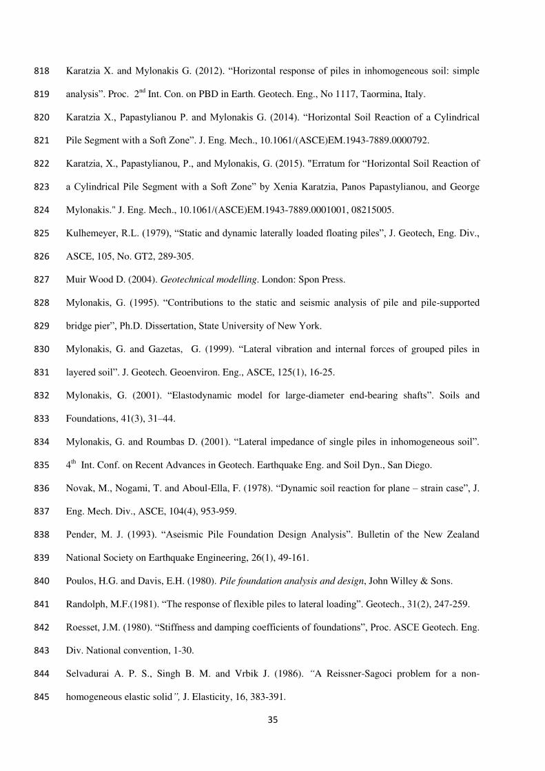
Λ = complex-valued dimensionless function of frequency 751
= shape parameter 752
v = soil Poisson’s ratio 753
= dimensionless parameter 754
ρs = soil mass density 755
σz = vertical normal stress 756
= polar angle in global reference system 757
φ(z) = normalized deflected shape of a fixed-head pile due to unit head rotation under zero 758
displacement 759
(z) = normalized deflected shape of a fixed-head pile due to unit head displacement under 760
zero rotation 761
i, j = any of the shape functions (z) and φ(z) 762
, L, 1, 2 = dimensionless coefficients 763
33
(z) = normalized deflected shape of a free-head pile due to a horizontal head force 764
= cyclic excitation frequency 765
766
ACKNOWLEDGEMENTS 767
The authors would like to acknowledge the contributions, in chronological order, of Mr. 768
Dimitri Roumbas, Dr. Costis Syngros, Ms. Alkisti Zina, Mr. Stefanos Drosos and Dr. Panos 769
Papastylianou, all former students of the senior author at the City University of New York 770
and University of Patras, in the development of the above method. Partial funding received 771
through a Caratheodory Program (B.388) at University of Patras is gratefully acknowledged. 772
773
REFERENCES 774
Abramowitz, M., and Stegun, I. A. (1965), Handbook of Mathematical Functions, U.S. National 775
Bureau of Standards (1964); Dover, New York 776
Anoyatis, G. and Mylonakis, G. (2012). “Dynamic Winkler Modulus for Axially Loaded Piles”, 777
Geotechnique, 62 (6), 521-536. 778
Anoyatis, G., Mylonakis, G. and Lemnitzer, A. (2016). “Soil reaction to lateral harmonic pile 779
motion”, J. Soil Dynamics and Earthquake Engineering, 87, 164-179. 780
Banerjee, P.K. and Davis, T.G. (1978). “The behaviour of axially and laterally loaded single piles 781
embedded in non – homogeneous soils”, Geotechnique, 28(3), 309-326. 782
Basu, D. and Salgado, R. (2008). “Analysis of laterally-loaded piles with rectangular cross sections 783
embedded in layered soil media”, Int. J. Num. Anal. Meth. Geomech., 32(7), 721-744. 784
Berger, E., Mahin, S. A., and Pyke, R. (1977), "Simplified Method for Evaluating Soil-Pile Structure 785
Interaction Effects," Proc., 9th Offshore Technology Conf., OTC Paper 2954, Houston, Tex., 589-598. 786
Bevington, P. R. and Robinson, D. K. (1992). “Data reduction and error analysis for the physical 787
sciences.” New York: McGraw Hill. 788
Blaney, G. W., Kausel, E., and Roesset, J. M. (1976), "Dynamic Stiffness of Piles," Proc. 2nd
Int. 789
Conf. Num. Meth. Geomech., Vol. II, Blacksburg, Virginia, June, 1001-1012. 790
34
Budhu, M, and Davis, T. G. (1987). “Nonlinear analysis of laterally loaded piles in cohesionless 791
soils”, Can. Geotech. J., 24, 289-296. 792
Clough R.. W. & Penzien, J. (1975). Structural Dynamics, McGraw-Hill. 793
Darendeli M. (2001). “Development of a new family of normalized modulus reduction and material 794
damping curves.” Ph.D. Thesis, Dept. of Civil Eng. University of Texas, Austin. 795
Di Laora, R. and Rovithis, E. (2015). “Kinematic bending of fixed-head piles in nonhomogeneous 796
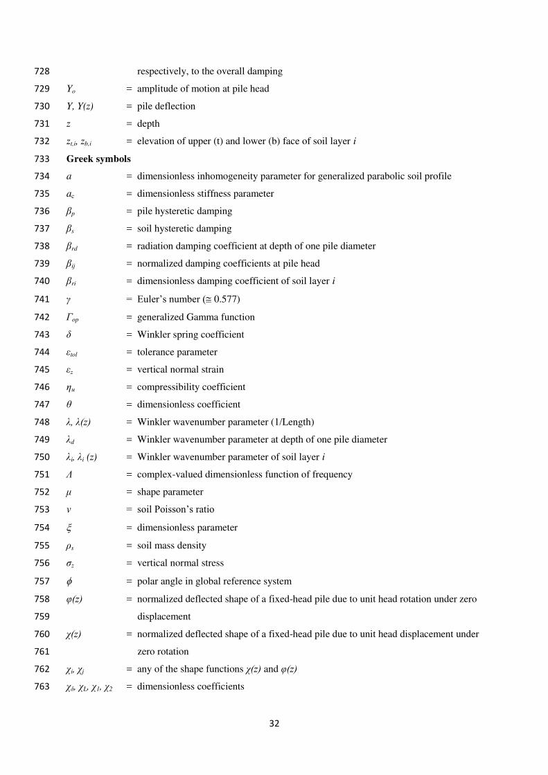
soil”, J. Geotech. Geoenviron. Eng. 141(4) 04014126, DOI: 10.1061/(ASCE) GT.1943-5606.0001270 797
Dobry, R., Vicente, E., O’Rourke, M. J., and Roesset, J. M. (1982).“Horizontal stiffness and damping 798
of single piles”, J. Geotech. Eng. Div., ASCE, Vol. 108, No. GT3, 439-459 799
El-Marsafawi, H., Kaynia, H.M., and Novak, M. (1992). “Interaction factors and the superposition 800
method for pile group dynamic analysis”, Report GEOT-1-92, GRC, Univ. Western Ontario, Canada. 801
Fleming, W.G.K., Weltman, A.J., Randolph, M.F., Elson, W.K. (1993). Piling Enineering, 2nd
802
Edition, John Wiley & Sons. 803
Gazetas, G. (1991). “Foundation Vibrations”, in Foundation Engineering Handbook, (H.Y. Fang, ed.), 804
Van Nostrand Reinholds, New York, 553-593. 805
Gazetas, G. and Dobry, R. (1984). “Horizontal response of piles in layered soils”. J. Geotech. Eng. 806
Div., ASCE, 110, 20-40. 807
Gazetas, G. and Mylonakis, G. (1998). “Seismic Soil-Structure Interaction: New Evidence and 808
Emerging Issues”, Geotechnical Special Publication No. 75, ASCE, 1119-1174. 809
Gerber M. T. and Rollins M. K. (2008). “Cyclic P-Y Curves for a Pile in Cohesive Soil.” Proc. Of 810
Geotech. Earthquake Eng. and Soil Dyn., IV, 1-10. 811
Gerolymos N. and Gazetas G. (2005b). “Phenomenological model applied to inelastic response of 812
soil–pile interaction systems”. Soils and Foundations, 45(4), 119–132. 813
Guo, W. (2012). Theory and Practice of Pile Foundations. London: CRC Press. 814
Hetenyi, M. (1946). Beams on elastic foundation, University of Michigan Press. 815
Kaynia, A. M., and Kausel, E. (1982). “Dynamic behaviour of pile groups”, Proc. of the 2nd Int. Conf. 816
on Numerical Methods in Offshore Piling, University of Texas at Austin, 509-531. 817
35
Karatzia X. and Mylonakis G. (2012). “Horizontal response of piles in inhomogeneous soil: simple 818
analysis”. Proc. 2nd
Int. Con. on PBD in Earth. Geotech. Eng., No 1117, Taormina, Italy. 819
Karatzia X., Papastylianou P. and Mylonakis G. (2014). “Horizontal Soil Reaction of a Cylindrical 820
Pile Segment with a Soft Zone”. J. Eng. Mech., 10.1061/(ASCE)EM.1943-7889.0000792. 821
Karatzia, X., Papastylianou, P., and Mylonakis, G. (2015). "Erratum for “Horizontal Soil Reaction of 822
a Cylindrical Pile Segment with a Soft Zone” by Xenia Karatzia, Panos Papastylianou, and George 823
Mylonakis." J. Eng. Mech., 10.1061/(ASCE)EM.1943-7889.0001001, 08215005. 824
Kulhemeyer, R.L. (1979), “Static and dynamic laterally loaded floating piles”, J. Geotech, Eng. Div., 825
ASCE, 105, No. GT2, 289-305. 826
Muir Wood D. (2004). Geotechnical modelling. London: Spon Press. 827
Mylonakis, G. (1995). “Contributions to the static and seismic analysis of pile and pile-supported 828
bridge pier”, Ph.D. Dissertation, State University of New York. 829
Mylonakis, G. and Gazetas, G. (1999). “Lateral vibration and internal forces of grouped piles in 830
layered soil”. J. Geotech. Geoenviron. Eng., ASCE, 125(1), 16-25. 831
Mylonakis, G. (2001). “Elastodynamic model for large-diameter end-bearing shafts”. Soils and 832
Foundations, 41(3), 31–44. 833
Mylonakis, G. and Roumbas D. (2001). “Lateral impedance of single piles in inhomogeneous soil”. 834
4th Int. Conf. on Recent Advances in Geotech. Earthquake Eng. and Soil Dyn., San Diego. 835
Novak, M., Nogami, T. and Aboul-Ella, F. (1978). “Dynamic soil reaction for plane – strain case”, J. 836
Eng. Mech. Div., ASCE, 104(4), 953-959. 837
Pender, M. J. (1993). “Aseismic Pile Foundation Design Analysis”. Bulletin of the New Zealand 838
National Society on Earthquake Engineering, 26(1), 49-161. 839
Poulos, H.G. and Davis, E.H. (1980). Pile foundation analysis and design, John Willey & Sons. 840
Randolph, M.F.(1981). “The response of flexible piles to lateral loading”. Geotech., 31(2), 247-259. 841
Roesset, J.M. (1980). “Stiffness and damping coefficients of foundations”, Proc. ASCE Geotech. Eng. 842
Div. National convention, 1-30. 843
Selvadurai A. P. S., Singh B. M. and Vrbik J. (1986). “A Reissner-Sagoci problem for a non-844
homogeneous elastic solid”, J. Elasticity, 16, 383-391. 845
36
Scott, R.F. (1981). Foundation analysis, Prentice Hall. 846
Syngros, C. (2004). Seismic response of piles and pile-supported bridge piers evaluated through case 847
histories. PhD Thesis, The City College and the Graduate Center of the City University of New York. 848
Tabesh, A., and Poulos, H. G. (2000). “A simple method for the seismic analysis of piles and its 849
comparison with the results of centrifuge tests.” Proc. of 12WCEE. 850
Veletsos A. S. and Younan A. H. (1995). “Dynamic Modeling and Response of Soil – Wall 851
Systems’’. J. Geotech. Eng., 120(12). 852
Vrettos, C. (1991). “Time-harmonic Boussinesq problem for a continuously non-homogeneous soil” 853
Earthquake Eng. Struct. Dyn., 20(10), 961–977. 854
855
(a) (b) (c) (d)
Fig. 1. a) Problem definition and active pile length, La; b) Unitary shape function for
pile deflection due to unit head displacement under zero rotation, (z); c)
Corresponding shape function due to unit head rotation under zero displacement, φ(z); d) Corresponding shape function due to unit head force under zero moment, (z).
10
z
(z)
0
z
φ(z)
1
3
4
Ep ,βp
dLa
Es ,βs
2
10
(z)
z
Y(z)
fixed head free head
a n
z / d
Es(z) / Esd
n = 0
Ho
mo
ge
ne
ou
s
0.5
n = 1
1
1
q = 1
0.30.1
b
Es(z) / Esd
q = 0
Ho
mo
ge
ne
ou
s
Exponential
Esihi
Multi-layer profile
z t,i
z b,i
Es1
Esn
1
1
z / d
a) b) c)
z
Generalizedparabolic
0.25
Fig. 2. Variation of soil stiffness with depth: (a) profile with unbounded parabolic
increase in stiffness according to Eq. 1; (b) profile with bounded exponential increase in
stiffness according to Eq. 6; (c) general multi-layer profile
Fig. 3. Radiation damping models (modified from Gazetas & Dobry 1984).
a0 = ωd / Vs
0.0 0.5 1.0
cr /
(dπρV
s)
0.0
1.0
2.0
3.0
4.0
5.0
6.0
7.0proposed model, v = 0.25
0.40
Gaz. & Dobry (1984), v =0.25
0.40
Novak et al (1978), v = 0.25
0.40
Tabesh & Poulos (2000)
a0 = ωd / Vs
0.0 0.5 1.0
analytical solution (Eq. 8b), v = 0.25
analytical solution (Eqn 12a), v 0.40
approximate (Eq. 10)
(a) (b)
Fig. 4. Comparison of Winkler radiation dashpot coefficient obtained with the proposed
model versus results from the literature, for two values of Poisson’s ratio.
Ep/Es
102 103 104 105
Win
kle
r m
od
ulu
s, δ
0.5
1.0
1.5
2.0
2.5
3.0
3.5proposed
Guo & Lee (2001)
Syngros (2004)
Dobry et al (1982)
fixed head1.2
Roesset (1980)
Ep/Es
102 103 104 105
proposed
Guo & Lee (2001)
Syngros (2004)
Gazetas & Dobry (1984)
free head
Fig. 5. Winkler modulus versus pile-soil stiffness contrast for long free- and fixed-head
piles in homogeneous soil; v = 0.4.
Ep/Esd
102 103 104 105
Win
kle
r m
od
ulu
s, δ
0.5
1.0
1.5
2.0
2.5
3.0
3.5proposed solution
Syngros (2004)
Homogeneous
Linear
Parabolic
fixed head
Ep/Esd
102 103 104 105
Homogeneous
Linear
free head
Parabolic
Fig. 6. Normalized Winkler modulus versus pile-soil stiffness contrast, for long fixed-
and free-head piles in different soil profiles; v = 0.4.
Ep/Esd
102 103 104
La/d
0
5
10
15
20
25
30
La/d
0
5
10
15
20
25
30
proposed (Eq. 26)
Gazetas (1991)
Syngros (2004)
Fleming et al (1993)
Budhu & Davies (1987)
Di Laora & Rovithis (2015)
Ep/Esd
102 103 104
Homogeneous profile Linear profile ( = , n = )
Parabolic profile (n = ) Exponential profile (b = , q = )
εtol = 103
εtol = 102
Fig. 7. Comparison of the proposed solution for active pile length La against results from
available solutions in the literature, for various soil profiles.
wr
rr
0.00
0.05
0.10
0.15
0.20
0.25
Srr
0.15
0.20
0.25
0.30
0.35
Shh
0.00
1.00
2.00
3.00
n = 0.25
0.5
1
wr
hh
0.00
0.25
0.50
0.75
Ep/Esd = 103
104
105
a
0.00.51.0
Shr
0.20
0.40
0.60
0.80
1.00
a
0.00.51.0
wr
hr
0.00
0.25
0.50
1/3
Fig. 8. Variation of coefficients Sij and wrij with inhomogeneity parameters a, n and soil-pile
stiffness contrast Ep/Esd, for a generalized parabolic profile.
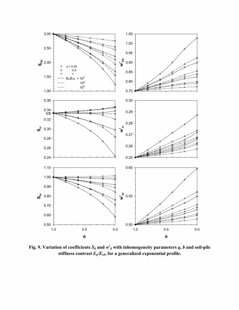
Sh
h
1.00
1.50
2.00
2.50
3.00
Ep/Esd = 103
104
105
wr
hh
0.75
0.80
0.85
0.90
0.95
1.00
1.05
q = 0.25
0.5
1
Srr
0.24
0.26
0.28
0.30
0.32
0.34
0.36
wr
rr
0.25
0.26
0.27
0.28
0.29
0.30
b
0.00.51.0
Sh
r
0.50
0.60
0.70
0.80
0.90
1.00
1.10
b
0.00.51.0
wr
hr
0.50
0.55
0.60
1/3
Fig. 9. Variation of coefficients Sij and wrij with inhomogeneity parameters q, b and soil-pile
stiffness contrast Ep/Esd, for a generalized exponential profile.
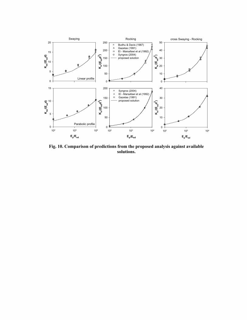
Ep/Esd
102 103 104
Krr/(Esdd3)
0
50
100
150
200
Krr/(Esdd3)
0
50
100
150
200
250
Ep/Esd
102 103 104
Khh/(Esdd)
0
5
10
15Syngros (2004)
El - Marsafawi et al (1992)
Gazetas (1991)
proposed solution
Khh/(Esdd)
0
5
10
15
20Budhu & Davis (1987)
Gazetas (1991)
El - Marsafawi et al (1992)
Syngros (2004)
proposed solution
Khr/(Esdd2)
0
10
20
30
40
50
Linear profile
Parabolic profile
Swaying Rocking
Ep/Esd
102 103 104
Khr/(Esdd2)
0
10
20
30
40
cross Swaying - Rocking
Fig. 10. Comparison of predictions from the proposed analysis against available
solutions.
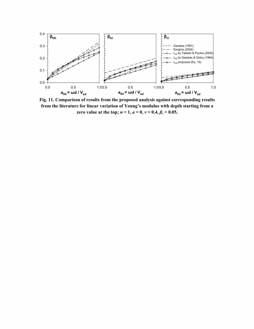
0.0 0.5 1.0
a0d
= ωd / Vsd
0.0 0.5 1.0
0.0
0.1
0.2
0.3
0.4
Gazetas (1991)
Syngros (2004)
crd by Tabesh & Poulos (2000)
crd by Gazetas & Dobry (1984)
crd proposed (Eq. 10)
0.0 0.5 1.0
a0d
= ωd / Vsd
a0d
= ωd / Vsd
βhh
βrr
βhr
Fig. 11. Comparison of results from the proposed analysis against corresponding results
from the literature for linear variation of Young’s modulus with depth starting from a
zero value at the top; n = 1, a = 0, v = 0.4, βs = 0.05.
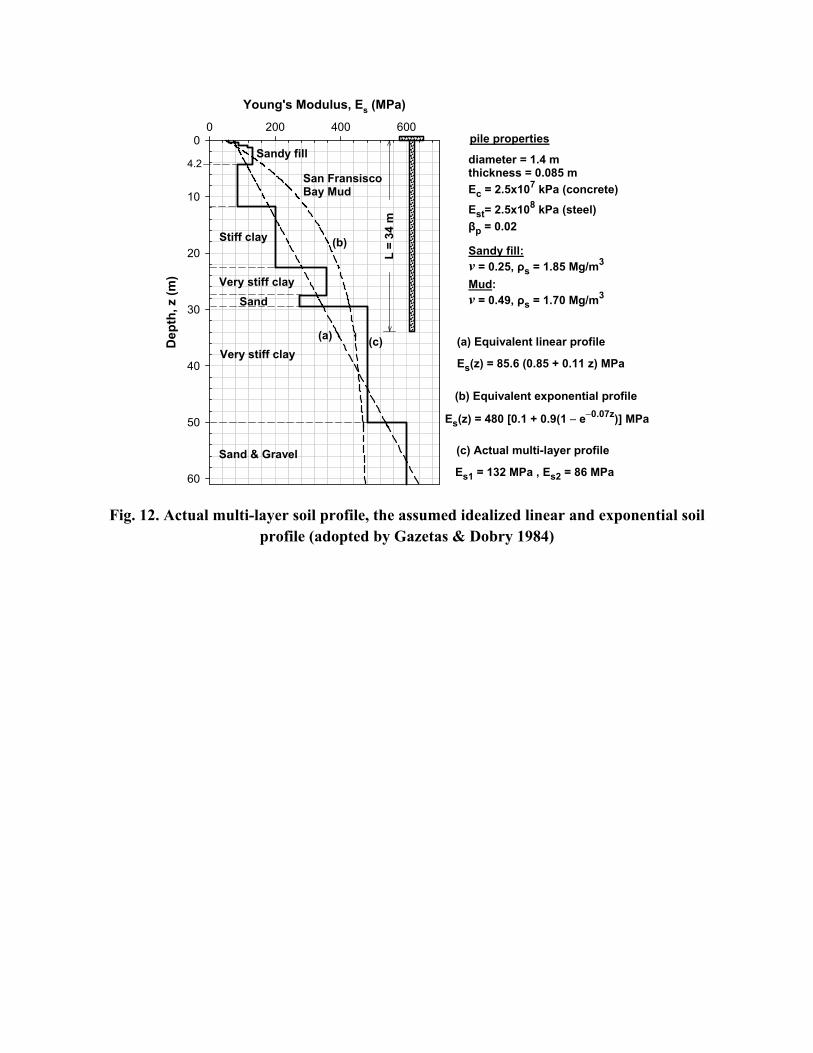
Young's Modulus, Es (MPa)
0 200 400 600
De
pth
, z (
m)
0
10
20
30
40
50
60
L =
34
m
Sandy fill
San Fransisco Bay Mud
Stiff clay
Very stiff clay
Sand
Very stiff clay
Sand & Gravel
diameter = 1.4 mthickness = 0.085 m
Ec = 2.5x10⁷ kPa (concrete)
Est= 2.5x10⁸ kPa (steel)
βp = 0.02
pile properties
4.2
(b) Equivalent exponential profile
(a) Equivalent linear profile
(c) Actual multi-layer profile
(c)
(b)
(a)
Sandy fill:
v = 0.25, ρs = 1.85 Mg/m3
Mud:
v = 0.49, ρs = 1.70 Mg/m3
Es(z) = 85.6 (0.85 + 0.11 z) MPa
Es(z) = 480 [0.1 + 0.9(1 e0.07z)] MPa
Es1 = 132 MPa , Es2 = 86 MPa
Fig. 12. Actual multi-layer soil profile, the assumed idealized linear and exponential soil
profile (adopted by Gazetas & Dobry 1984)
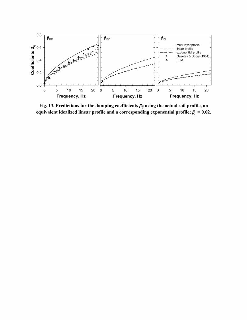
Frequency, Hz
0 5 10 15 20
βrr
Frequency, Hz
0 5 10 15 20
βhr
Frequency, Hz
0 5 10 15 20
Co
eff
icie
nts
βij
0.0
0.2
0.4
0.6
0.8
multi-layer profile
linear profile
exponential profile
Gazetas & Dobry (1984)
FEM
βhh
Fig. 13. Predictions for the damping coefficients βij using the actual soil profile, an
equivalent idealized linear profile and a corresponding exponential profile; βp = 0.02.
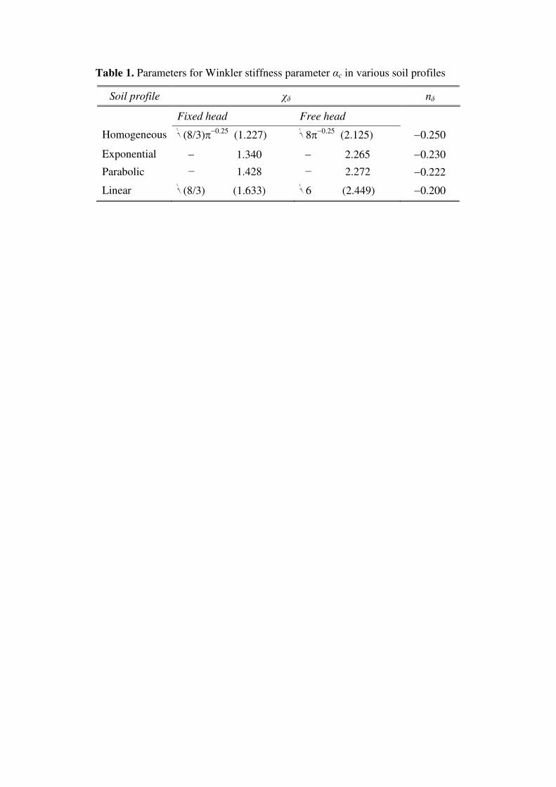
Table 1. Parameters for Winkler stiffness parameter αc in various soil profiles
Soil profile χδ nδ
Fixed head Free head
Homogeneous (8/3)0.25 (1.227) 80.25
(2.125) 0.250
Exponential 1.340 2.265 0.230
Parabolic − 1.428 − 2.272 0.222
Linear (8/3) (1.633) 6 (2.449) 0.200
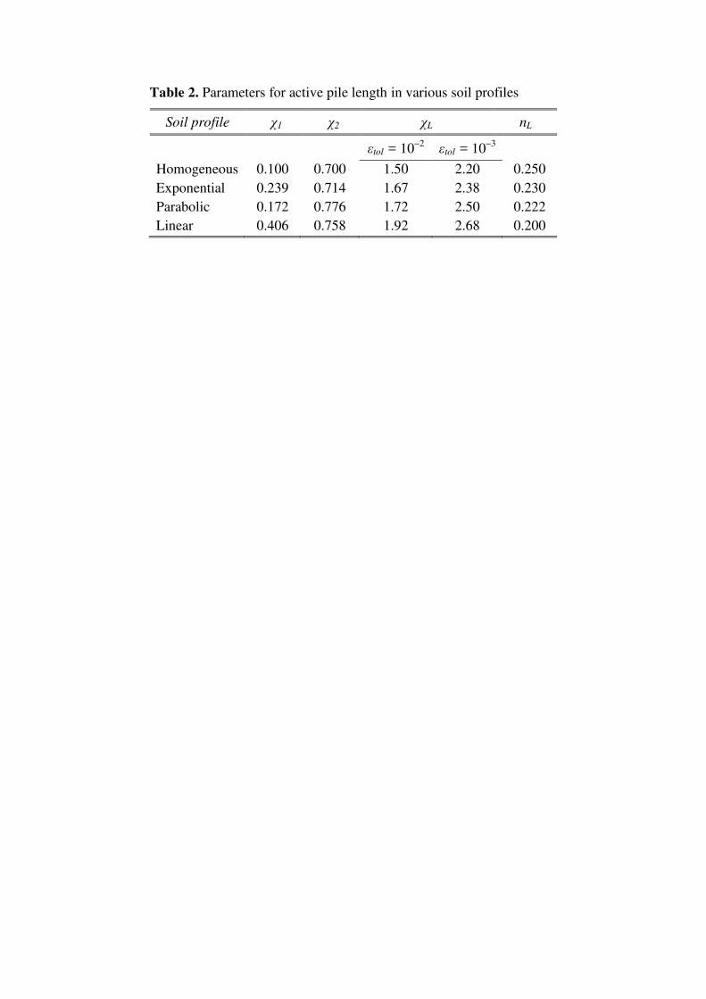
Table 2. Parameters for active pile length in various soil profiles
Soil profile χ1 χ2 χL nL
εtol = 102
εtol = 103
Homogeneous 0.100 0.700 1.50 2.20 0.250
Exponential 0.239 0.714 1.67 2.38 0.230
Parabolic 0.172 0.776 1.72 2.50 0.222
Linear 0.406 0.758 1.92 2.68 0.200