Keeping Two Sets of Books: The Relationship Between

Tax & Incentive Transfer Prices

Charles E. Hyde*

Deloitte Touche Tohmatsu and University of Melbourne

PO Box N250, Grosvenor Place 225 George Street, Sydney

NSW, 1217, Australia

Email: chyde@deloitte.com.au

May 24, 2002

J.E.L. Classifications: H26, H73, H87.

Running Title: The Relationship Between Tax and Incentive Transfer Prices * I wish to thank Deloitte colleagues in Toronto and Sydney for their valuable comments.

Abstract Multinationals can use different prices for cost and tax accounting purposes. We study how both transfer prices are set under the separate entity and formula apportionment approaches to taxation. The effect of penalties for noncompliance with arm’s length pricing on the relationship between the two prices is also examined. The results are sensitive to whether the cost accounting price is dictated or negotiated, but robust to alternative market structures and imperfect taxation. Our results highlight the need for firms and governments to take an integrated approach to formulating transfer pricing policy that recognizes the distinct but related roles of the two transfer prices.

1

1. Introduction Transfer prices serve two distinct roles within multinational enterprises (MNEs).

They affect the incentives of divisional managers who are remunerated on the basis of

their division’s performance. Second, transfer prices determine the tax liability of each

division, thus affecting the overall tax exposure of the MNE. While the incentive

literature is relevant to all multidivisional firms, the tax literature applies only to the

subset of multidivisional firms that are also multinational. Despite this being a sizeable

and growing segment of the global economy, to a large extent these two distinct roles of

transfer prices have been examined more or less in isolation.

Studies of the managerial incentive implications of transfer prices include Harris,

Kriebel and Raviv (1982), Amershi and Cheng (1990), Holmstrom and Tirole (1991), and

Anctil and Dutta (1999). The literature examining the implications of tax regulations

governing the pricing of intrafirm transactions across sovereign jurisdictions includes

Musgrave (1973), Gordon and Wilson (1986), Kant (1988, 1990), Bucks and Mazerof

(1993), and Goolsbee and Maydew (2000). Other papers have taken an integrated

approach, explicitly recognizing both (managerial) incentive and tax considerations in

deriving optimal transfer prices (Halperin and Srinidhi, 1991; Elitzur and Mintz, 1996;

Schjelderup and Sorgard, 1997; Sansing, 1999; Haufler and Schjelderup, 2000; Smith,

2000).

In all of the studies above, however, the MNE is assumed to nominate only one

transfer price per intrafirm transaction. In effect, these models implicitly require that the

tax transfer price do ‘double duty’ by also serving as an incentive mechanism.

Equivalently, they implicitly assume that MNEs keep only one set of books to satisfy

both cost and tax accounting requirements. Given that there is no statutory requirement

in the US or many other countries that the incentive and tax transfer prices are the same,

this assumption seems unwarranted. After all, logic dictates that MNEs can do better

using two prices, rather than one, to pursue the two distinct goals of optimizing

managerial incentives and minimizing tax (inclusive of expected penalties).

2

It might be argued that this criticism is academic since a study in the early 1980’s

showed that most MNEs do not employ separate transfer prices for incentive and tax

purposes.1 However, a more recent survey suggests that MNEs may now be more

inclined to nominate two different transfer prices (Ernst & Young, 1999). It is certainly

plausible that the increased scrutiny by tax authorities in the last twenty years will have

led more MNEs to recognize the benefit of employing different transfer prices.2 This

perspective is the distinguishing feature of our model – the MNE simultaneously chooses

separate tax and incentive transfer prices, fully recognizing their interrelatedness.

Baldenius, Melamud and Reichelstein (2002) have also modeled two distinct transfer

prices in concurrent research, although the focus of their analysis differs markedly.3

We ask five separate questions. First, does the relationship between the optimal tax

and incentive transfer prices depend on whether the separate entity or formula

apportionment approaches are used to determine taxable income?4 Second, focusing on

the former approach, how do changes in the tax and cost environment affect the

relationship? Third, do the answers to the second question depend importantly upon

whether the incentive transfer price is dictated by one affiliate or negotiated by both

parties? Fourth, what are the implications of oligopoly vis-à-vis monopoly for the

relationship between the two transfer prices, and lastly is it affected by double or ‘less

than single’ taxation?5

1 Czechowicz, et al., (1982) reported that 89% of U.S. MNE’s use the same transfer price for incentive and tax purposes. Additionally, they reported that some MNE’s felt that tax authorities would be antagonistic toward the use of two different transfer prices. 2 As tax transfer pricing regulations become more narrowly defined and effectively enforced, MNEs that employ only one transfer price will find it increasingly difficult to implement the price that optimally trades off both tax and strategic considerations. 3 They examine how the managerial incentive transfer should be set given a range of admissible tax transfer prices. They focus on both market- and cost-based transfer pricing and examine how intracompany discounts are affected. 4 Formula apportionment refers to the use of a formula based on consolidated sales, assets, payroll and possibly other factors to allocate consolidated taxable income among an MNE’s affiliates. In contrast, the separate entity approach treats each affiliate of the MNE as if it were an independent, “arm’s length” entity for determining taxable income. This approach is embraced by the OECD and is effectively the global standard for international transfer pricing (OECD, 1995). Others have referred to this as the ‘separate accounting’ approach – our terminology is consistent with OECD usage and, we feel, more suggestive. 5 The term ‘less than single taxation’ is the opposite of double taxation – it refers to the situation where some income is not taxed in either jurisdiction.

3

We assume decentralized decision making in the sense that the subsidiary determines

the amount it purchases from its parent.6 However, the parent has a first-mover

advantage in that it sets the transfer price first and then the subsidiary reacts.7 The

subsidiary maximizes its own, rather than consolidated, after-tax profit.8 Both the

subsidiary and the parent are initially assumed to be monopolists in their own market –

this assumption is later relaxed – and penalties are imposed for noncompliance with

arm’s length pricing.

Under the formulary apportionment (FA) approach we show that the two transfer

prices are independent, regardless of whether penalties for non-arm’s length pricing are

applied or not. This stems from the fact that there is no role for a tax transfer price under

this approach – the taxable income of each entity is instead calculated as an exogenously

defined fraction of consolidated taxable income.

In contrast, under the separate entity (SE) approach the two transfer prices are shown

to be very much interdependent. To illustrate, changes in the tax environment are shown

to affect both the tax and incentive transfer prices. As the penalty for noncompliance

with arm’s length pricing (or the probability of being penalized) increases, naturally a

more conservative tax transfer price is adopted. Also, the incentive transfer price adjusts

so as to cushion the effect of the tax transfer price adjustment on the subsidiary’s related-

party purchases. This highlights an important result: changes in the tax environment have

implications for the incentive transfer price.

A change in the MNE’s cost structure is also shown to affect both transfer prices.

Assuming the parent faces a lower tax rate than the subsidiary, an increase in the parent’s

marginal cost of production causes the incentive transfer price to increase and the tax

6 Subsidiaries often have considerable autonomy in decision-making. In fact, it is not uncommon for the subsidiary and parent to negotiate transfer prices. See the discussion in section 2.2. 7 Our model differs from Nielsen, et al. (2001a) in that we assume the parent determines its domestic sales quantity at the same time as the transfer prices, thus meaning that it sets its quantity prior to the subsidiary – they assume the parent and subsidiary quantities to be determined simultaneously. Given that they compete in different markets, this difference seems unimportant. 8 This need not be detrimental to the parent in an oligopolistic setting, due to the potential benefits of delegation (Vickers, 1985). See Elitzur and Mintz (1996) for an analysis of transfer pricing in the context of unobservable managerial effort.

4

transfer price to decrease. The former induces the subsidiary to purchase less from the

parent, an efficient response given that the good has become more costly to produce. The

decrease in the tax transfer price reinforces this incentive as a lower tax transfer price

results in a higher taxable income, and thus tax payable, for the subsidiary. Because this

effect is in proportion to the amount purchased, it is equivalent to an increase in the

subsidiary’s marginal cost.

Thus, changes in both the tax environment and the technology have implications for

both transfer pricing policies – incentive and tax. The fact that the effect on each price

differs establishes the need to distinguish between the two transfer prices. This also

points to the need for an integrated approach to government tax and industry policy. For

example, our results imply that an output subsidy that affects production costs will not

only impact upon the incentive policy of a MNE, but also their tax policy. If it induces

the MNE to distort their tax transfer price even further from the arm’s length price,

governments may need to link the subsidy to increased transfer pricing penalties and tax

audit activity.

Whether the incentive transfer price is negotiated or dictated (by the parent) also

impacts upon the relationship between the two transfer prices. Specifically, if the

subsidiary has sufficient bargaining power, then the incentive transfer price is

independent of the tax transfer price due to the fact that the former will always be set at

zero – a corner solution. This illustrates the importance of understanding the objectives

of each affiliate and the distribution of price-setting power within the MNE group.

Our earlier results under dictated pricing, however, are shown to be robust in the sense

of being invariant to market structure. Specifically, they hold provided the law of

demand is satisfied for intra-firm trade. The reason is that, while strategic rivalry needs

to be taken into consideration in oligopolistic settings, the incentive role of the incentive

transfer price remains essentially unchanged. Similarly, the earlier results are also shown

to be unaffected by less than single or double taxation – both are very real possibilities,

motivating the many international tax treaties in existence today. While impacting upon

5

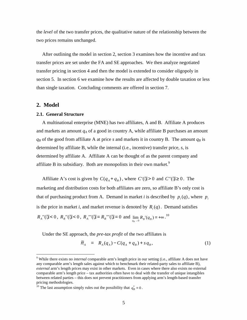
the level of the two transfer prices, the qualitative nature of the relationship between the

two prices remains unchanged.

After outlining the model in section 2, section 3 examines how the incentive and tax

transfer prices are set under the FA and SE approaches. We then analyze negotiated

transfer pricing in section 4 and then the model is extended to consider oligopoly in

section 5. In section 6 we examine how the results are affected by double taxation or less

than single taxation. Concluding comments are offered in section 7.

2. Model 2.1. General Structure

A multinational enterprise (MNE) has two affiliates, A and B. Affiliate A produces

and markets an amount qA of a good in country A, while affiliate B purchases an amount

qB of the good from affiliate A at price s and markets it in country B. The amount qB is

determined by affiliate B, while the internal (i.e., incentive) transfer price, s, is

determined by affiliate A. Affiliate A can be thought of as the parent company and

affiliate B its subsidiary. Both are monopolists in their own market.9

Affiliate A’s cost is given by )( BA qqC + , where 0)( >⋅C' and 0)( ≥⋅C'' . The

marketing and distribution costs for both affiliates are zero, so affiliate B’s only cost is

that of purchasing product from A. Demand in market i is described by )(qpi , where ip

is the price in market i, and market revenue is denoted by )(qRi . Demand satisfies

0)( <⋅''RA , 0)( <⋅''RB , 0)()( =⋅=⋅ '''R'''R BA and +∞=→

)(lim0 BBq

q'RB

.10

Under the SE approach, the pre-tax profit of the two affiliates is

,)()(~BBAAAA qsqqCqR ++−=π (1)

9 While there exists no internal comparable arm’s length price in our setting (i.e., affiliate A does not have any comparable arm’s length sales against which to benchmark their related-party sales to affiliate B), external arm’s length prices may exist in other markets. Even in cases where there also exists no external comparable arm’s length price – tax authorities often have to deal with the transfer of unique intangibles between related parties – this does not prevent practitioners from applying arm’s length-based transfer pricing methodologies. 10 The last assumption simply rules out the possibility that 0* =Bq .

6

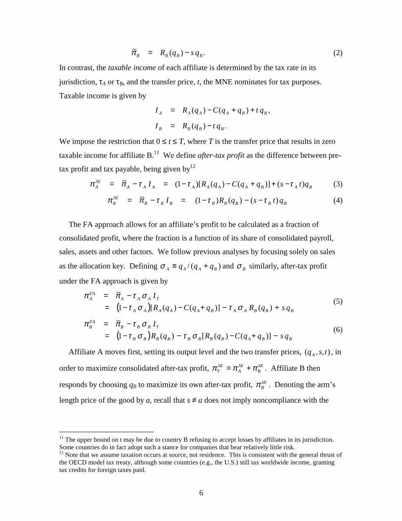
.)(~BBBB qsqR −=π (2)

In contrast, the taxable income of each affiliate is determined by the tax rate in its

jurisdiction, τA or τB, and the transfer price, t, the MNE nominates for tax purposes.

Taxable income is given by

,)()( BBAAAA qtqqCqRI ++−=

.)( BBBB qtqRI −=

We impose the restriction that 0 ≤ t ≤ T, where T is the transfer price that results in zero

taxable income for affiliate B.11 We define after-tax profit as the difference between pre-

tax profit and tax payable, being given by12

BABAAAAAAASEA qtsqqCqRI )()]()()[1(~ τττππ −++−−=−= (3)

BBBBBBBBSEB qtsqRI )()()1(~ τττππ −−−=−= (4)

The FA approach allows for an affiliate’s profit to be calculated as a fraction of

consolidated profit, where the fraction is a function of its share of consolidated payroll,

sales, assets and other factors. We follow previous analyses by focusing solely on sales

as the allocation key. Defining )(/ BAAA qqq +≡σ and Bσ similarly, after-tax profit

under the FA approach is given by

( ) BBBAABAAAAA

TAAAFAA

qsqRqqCqRI

+−+−−=−=

)()]()([1

~

στστστππ

(5)

( ) BBABBBBBBBB

TBBBFAB

qsqqCqRqRI

−+−−−=−=

)]()([)(1

~

στστστππ

(6)

Affiliate A moves first, setting its output level and the two transfer prices, ),,( tsqA , in

order to maximize consolidated after-tax profit, SEB

SEA

SET πππ += . Affiliate B then

responds by choosing qB to maximize its own after-tax profit, SEBπ . Denoting the arm’s

length price of the good by a, recall that s ≠ a does not imply noncompliance with the

11 The upper bound on t may be due to country B refusing to accept losses by affiliates in its jurisdiction. Some countries do in fact adopt such a stance for companies that bear relatively little risk. 12 Note that we assume taxation occurs at source, not residence. This is consistent with the general thrust of the OECD model tax treaty, although some countries (e.g., the U.S.) still tax worldwide income, granting tax credits for foreign taxes paid.

7

arm’s length principle – this occurs only if t ≠ a.13 We use backwards induction to solve

for the subgame perfect Nash equilibrium.

2.2. Organizational Structure

The parent (affiliate A) delegates responsibility to the subsidiary (affiliate B) for

determining the quantity the latter purchases. In addition, the subsidiary seeks to

maximize its own (not parent) profit. Although the parent indirectly controls the

subsidiary’s purchase level through its pricing of the product, this loss of (direct) control

over quantity is to the parent’s detriment. Given that the parent wholly owns the

subsidiary, this raises the question of why the parent doesn’t dictate the quantity.

We begin by noting that our model accurately describes reality – while the parent

often sets the transfer price, rarely will it also dictate the amount of product to be sold to

its subsidiaries. The reason for this would appear to be the informational asymmetries a

parent faces in assessing offshore market conditions. Thus, there are two pertinent

questions. First, why not model these information asymmetries? Second, why assume

that subsidiary management acts to maximize subsidiary, rather than consolidated, profit?

After all, to solve the incentive misalignment problem the parent need only tie subsidiary

management compensation to group profit.

While the incorporation of information asymmetries into this model is a natural next

step, we omit them here in order to render a tractable benchmark model. On the second

question, the theory of moral hazard provides a reason for not tying the compensation of

subsidiary management to consolidated profit. Since consolidated profit depends on the

performance of the parent and all of its subsidiaries, tying management’s compensation

to consolidated profit means rewarding them based on the performance of entities over

which they exert no control. This dulls their incentive to undertake costly actions to

improve the performance of their own subsidiary, as they can free-ride on the efforts of

the parent and the other subsidiaries. Thus, the parent suffers a loss of control, resulting

13 Under perfectly competitive conditions, a equals the marginal cost of production. Under all other market structures a is more difficult to determine, depending upon the degree of buyer and seller market power. In reality, tax authorities define a range of acceptable prices, usually the interquartile range obtained from analyzing a set of comparable firms.

8

in an attendant loss of subsidiary performance. Indeed, in practice managers are usually

remunerated against divisional performance and this has been recognized in the literature

(Elitzur and Mintz, 1996; Baldenius, et al., 2002).

3. Separate Entity and Formula Apportionment Approaches

Regardless of which approach is used, in order to determine affiliate A’s transfer

pricing strategy we must first determine how affiliate B responds to any given pair of

transfer prices. Affiliate A takes this anticipated reaction into account in determining

how to optimally set the two transfer prices.

3.1. Formula Apportionment Approach

Inspecting Equation (6) it is clear that affiliate B’s after-tax profit depends on s but not

t. While the latter ensures 0/* =dtdqB , concavity of affiliate B’s after-tax profit function

also gives 0/* <dsdqB – that is, the law of demand holds. Although consolidated after-

tax profit, FAB

FAA

FAT πππ += , does not depend directly on either s or t, it does depend

indirectly on s through the functional relationship )(* sqB . It follows that affiliate A, while

having a strict preference over the level of the incentive transfer price, is indifferent

between all tax transfer prices. Hence, there is no loss to assuming that affiliate A always

sets the tax transfer price equal to the arm’s length price.

In the presence of penalties for non-arm’s length pricing, affiliate A clearly has a strict

preference for setting t = a. Quite simply, there is no rationale for penalties for

noncompliance with arm’s length pricing under the FA approach since, as we have

shown, there is no role for the tax transfer price to play. To conclude, under the FA

approach only the incentive transfer price has a non-trivial role to play.

Proposition 1. Under formula apportionment the tax and incentive transfer prices are independent.

Since we are interested here in understanding the relationship between the two transfer

prices, we henceforth restrict attention to the SE approach.

9

3.2. Separate Entity Approach

Affiliate B’s after-tax profit is now given by Equation (4) and it can be shown that

0)()1(

1*

<−

=BBB

B

q"Rdsdq

τ, (7)

0)()1(

*

>−

−=

BBB

BB

q"Rdtdq

ττ

. (8)

Now affiliate B is affected by both transfer prices. While an increase in s still decreases

affiliate B’s purchases, it now benefits from an increase in t as this reduces its taxable

income and thus also tax payable. A higher tax transfer price essentially acts as a subsidy

by lowering B’s effective marginal cost and thus inducing it to purchase more.

Turning to affiliate A’s decision making, consolidated after-tax profit is given by

),(][)),(()1(

))],(()()[1(tsqttsqR

tsqqCqR

BBABBB

BAAAASET

ττττπ

−−−++−−=

(9)

Affiliate A now has a clear incentive to distort the tax transfer price because it directly

impacts upon consolidated after-tax profit. In fact, it is straightforward to show that we

obtain a corner solution, where },0{ Tt ∈ . Quite simply, it should seek to shift as much

taxable income as possible into the low tax jurisdiction. This idea is not new, being

central to most discussions, both practical and theoretical, of transfer pricing.

Thus, in the absence of penalties MNE incentives in regards to tax transfer pricing can

be understood without reference to incentive transfer pricing. In reality, however, MNEs

that engage in non-arm’s length transfer pricing are exposed to the risk of penalties by the

tax authority whose revenue base has been eroded.14

To capture this, suppose now that the MNE has some probability of being penalized an

amount P > 0 when choosing a non-arm’s length tax transfer price – penalties are applied

to after-tax profit. To simplify the analysis, we restrict attention to the case where τA <

14 The realities of penalty exposure are complicated and we do not attempt a full exposition here. It is worth noting, though, that tax authorities typically make adjustments to transfer prices deemed not to be arm’s length. This possibility is not explicitly factored into our model, although such adjustments could possibly be viewed as being implicitly embedded in the penalty.

10

τB, in which case the MNE has an incentive to use high tax transfer prices to shift profit

from country B to country A.15 The probability that affiliate B is penalized is described

by the cumulative distribution function F(t– a), where F(0) = 0 and F( a – a) = 1. Thus,

a is a threshold transfer price in the sense that if at > , then affiliate B is penalized with

certainty. The associated probability distribution function is denoted f(t – a), satisfying

0)0( =f and 0)( >⋅'f .16

Consolidated after-tax profit is now given by

PatFtsqttsqRtsqqCqR

BBA

BBBBAAAASET

)(),(][)),(()1())],(()()[1(

−−−−−++−−=

ττττπ

(10)

The first-order conditions describing the profit-maximizing values ),,( ***Aqst are

[ ] 0)()()()1()1(:*

=−−−−−−−−− PatfqtC''Rdt

dqt BBABAABBB ττττττ (11)

[ ] 0)()1()1(:*

=−−−−− tC''Rds

dqs BAABBB ττττ , (12)

0][)1(: =−− C''Rq AAA τ . (13)

Provided the penalty, P, is sufficiently high, affiliate A’s profit maximizing tax

transfer price is now characterized by an interior solution – that is, affiliate A does not

attempt to shift as much income as possible to the low tax jurisdiction. To see this note

that the expression in square brackets in Equation (12) must equal zero, implying that

Equation (11) reduces to

PatftsqBAB )(),(][ −=−ττ . (11’)

The optimal tax transfer price cannot satisfy t ≤ a since this ensures that the right hand

side of Equation (11’) is zero while, recalling footnote 11 and the restriction τA < τB, we

know that the left hand side is strictly positive. On the other hand, for all t ≥ a , if the

penalty is sufficiently high – see Assumption 1(a) below and footnote 19 – then the right

15 The same arguments apply if instead τA > τB. 16 Note that 0>'f implies that as t increases, the probability of being penalized increases at an increasing rate. This seems plausible and perhaps even likely.

11

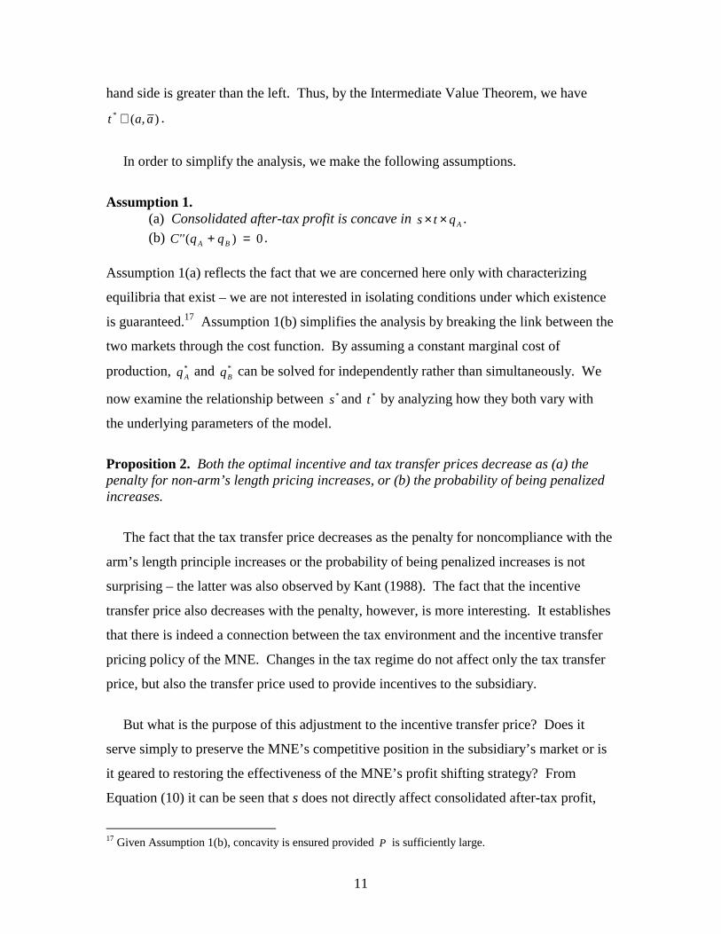
hand side is greater than the left. Thus, by the Intermediate Value Theorem, we have

),(* aat ∈ .

In order to simplify the analysis, we make the following assumptions.

Assumption 1. (a) Consolidated after-tax profit is concave in Aqts ×× . (b) 0)( =+ BA qqC'' .

Assumption 1(a) reflects the fact that we are concerned here only with characterizing

equilibria that exist – we are not interested in isolating conditions under which existence

is guaranteed.17 Assumption 1(b) simplifies the analysis by breaking the link between the

two markets through the cost function. By assuming a constant marginal cost of

production, *Aq and *

Bq can be solved for independently rather than simultaneously. We

now examine the relationship between *s and *t by analyzing how they both vary with

the underlying parameters of the model.

Proposition 2. Both the optimal incentive and tax transfer prices decrease as (a) the penalty for non-arm’s length pricing increases, or (b) the probability of being penalized increases.

The fact that the tax transfer price decreases as the penalty for noncompliance with the

arm’s length principle increases or the probability of being penalized increases is not

surprising – the latter was also observed by Kant (1988). The fact that the incentive

transfer price also decreases with the penalty, however, is more interesting. It establishes

that there is indeed a connection between the tax environment and the incentive transfer

pricing policy of the MNE. Changes in the tax regime do not affect only the tax transfer

price, but also the transfer price used to provide incentives to the subsidiary.

But what is the purpose of this adjustment to the incentive transfer price? Does it

serve simply to preserve the MNE’s competitive position in the subsidiary’s market or is

it geared to restoring the effectiveness of the MNE’s profit shifting strategy? From

Equation (10) it can be seen that s does not directly affect consolidated after-tax profit,

17 Given Assumption 1(b), concavity is ensured provided P is sufficiently large.

12

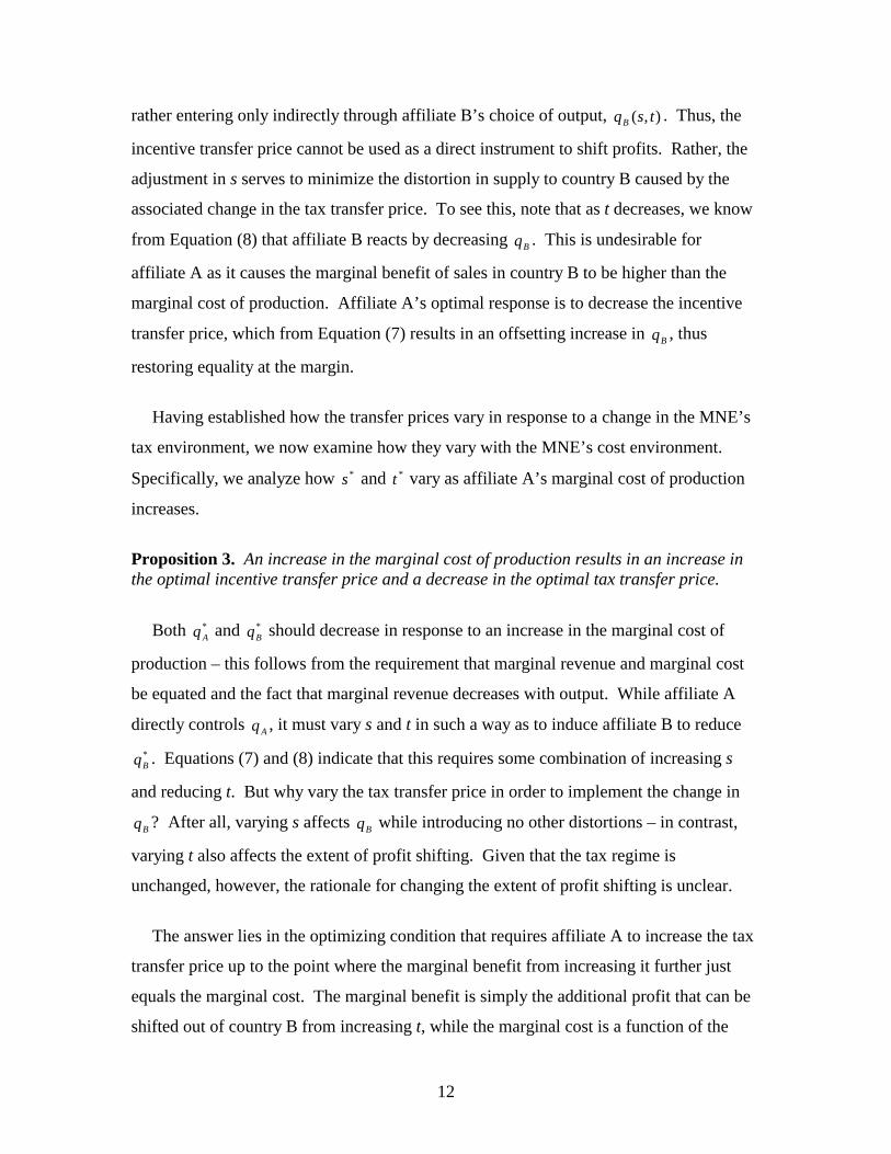
rather entering only indirectly through affiliate B’s choice of output, ),( tsqB . Thus, the

incentive transfer price cannot be used as a direct instrument to shift profits. Rather, the

adjustment in s serves to minimize the distortion in supply to country B caused by the

associated change in the tax transfer price. To see this, note that as t decreases, we know

from Equation (8) that affiliate B reacts by decreasing Bq . This is undesirable for

affiliate A as it causes the marginal benefit of sales in country B to be higher than the

marginal cost of production. Affiliate A’s optimal response is to decrease the incentive

transfer price, which from Equation (7) results in an offsetting increase in Bq , thus

restoring equality at the margin.

Having established how the transfer prices vary in response to a change in the MNE’s

tax environment, we now examine how they vary with the MNE’s cost environment.

Specifically, we analyze how *s and *t vary as affiliate A’s marginal cost of production

increases.

Proposition 3. An increase in the marginal cost of production results in an increase in the optimal incentive transfer price and a decrease in the optimal tax transfer price.

Both *Aq and *

Bq should decrease in response to an increase in the marginal cost of

production – this follows from the requirement that marginal revenue and marginal cost

be equated and the fact that marginal revenue decreases with output. While affiliate A

directly controls Aq , it must vary s and t in such a way as to induce affiliate B to reduce *Bq . Equations (7) and (8) indicate that this requires some combination of increasing s

and reducing t. But why vary the tax transfer price in order to implement the change in

Bq ? After all, varying s affects Bq while introducing no other distortions – in contrast,

varying t also affects the extent of profit shifting. Given that the tax regime is

unchanged, however, the rationale for changing the extent of profit shifting is unclear.

The answer lies in the optimizing condition that requires affiliate A to increase the tax

transfer price up to the point where the marginal benefit from increasing it further just

equals the marginal cost. The marginal benefit is simply the additional profit that can be

shifted out of country B from increasing t, while the marginal cost is a function of the

13

expected penalty. As *s increases this causes *Bq to fall, which in turn decreases the

marginal benefit from varying t – the smaller volume of trade means the tax transfer price

now has less leverage. While the marginal benefit from increasing t is now lower than

what it was before the increase in marginal cost of production, the marginal cost

associated with increasing t remains unchanged since the expected penalty remains as it

was before. Profit maximization thus requires affiliate A to make a downward

adjustment to the tax transfer price.

Thus, the relationship between the two transfer prices can be complicated and difficult

to anticipate. Depending on the nature of the change in the MNE’s economic

environment, the prices may move in the same direction or in opposite directions. Also,

the change in the tax transfer price may drive, or be driven by, the associated change in

the incentive transfer price. Models that do not distinguish between the two transfer

prices necessarily fail to appreciate these possibilities and complexities.

4. Negotiated Transfer Pricing

So far we have assumed that affiliate A unilaterally determines both transfer prices. It

is not uncommon, however, for affiliates to negotiate over the incentive transfer price –

this is true even where one of the parties is the parent company. Indeed, it would be no

exaggeration to say that negotiation is the norm rather than the exception (Vaysman,

1985; p. 910 of Horngren, Foster and Datar, 1997). This suggests that the ‘hold-up

problem’ paradigm may also be an appropriate perspective for analyzing internal

transactions (Williamson, 1985; Grossman and Hart, 1986; Holmstrom and Tirole, 1991).

We now examine how our previous results are affected if the incentive transfer price is

negotiated rather than dictated.

The approach we employ to modeling the outcome of the negotiations differs from

that used by Baldenius, et al. (1998). While they postulate some fixed surplus over which

the entities bargain in a zero-sum game, there exists no such clearly defined surplus in

14

our setting.18 Indeed, whatever profit affiliate B obtains is also enjoyed by affiliate A

since the parent cares about the welfare of its subsidiary. We parameterize affiliate A’s

bargaining power by ]1,0[∈γ , where the negotiated price, s~ , is defined by SEB

SEA

s

SEB

SET

ss ππγπγπγ +=−+= maxarg)1(maxarg~ .

Note that if 1=γ , then *~ ss = . That is, they agree on the incentive transfer price that is

optimal for affiliate A. Similarly, if 0=γ , then the negotiated price is the one that

maximizes affiliate B’s welfare.

We assume that the timing is as before – they negotiate over the incentive transfer

price at the same time as affiliate A determines the tax transfer price and the quantity to

sell in its own market. Affiliate B then responds by choosing its quantity, Bq . The

conditions describing the equilibrium ),~,( **Aqst are now given by Equations (11), (12’)

and (13), where

[ ] 0)()1()1(:~*

=−−−−− tC''Rds

dqs BAABBB τττγτ (12’)

We now establish that the results of section 3 are robust in the following sense. Proposition 4. (a) If affiliate A’s bargaining power is sufficiently strong, then Propositions 2 and 3 also

hold when the incentive transfer price is negotiated. (b) If affiliate A’s bargaining power is sufficiently weak, then the negotiated incentive

transfer price is independent of the penalty and cost environment, while the tax transfer price varies according to Propositions 2 and 3.

This result shows that the relationship between the cost/tax structure and the transfer

prices depends importantly on organizational features of the MNE – in particular, the

relative bargaining power of the affiliates over the internal pricing of product. The

intuition for part (a) is that if affiliate A exerts considerable power over the level of the

incentive transfer price, then the decision problem is essentially the same as that

considered in the previous section where affiliate A unilaterally determined this price. In

18 Their approach is perhaps more appropriate for understanding negotiations between sister companies, who have no reason to be concerned for the other’s welfare – indeed, to some extent they may vigourously compete for fixed parent resources.

15

particular, both the incentive and tax transfer equilibrium prices continue to be defined by

an interior solution and the factors affecting these prices remain the same.

On the other hand, if affiliate B exerts considerable control over the incentive transfer

price, then their preference is naturally to set the price as low as possible – at zero.

Because this is a corner solution, the negotiated price is then invariant to perturbations in

the penalty regime or affiliate A’s marginal cost of production. The asymmetry in the

model properties across the two extremes of bargaining power simply reflects the

different pricing incentives facing the two affiliates and the mathematical fact that

interior solutions are more easily perturbated than corner solutions. The properties of the

negotiated transfer price for intermediate levels of bargaining power are less clear, due to

the possible existence of non-convexities in the objective function defining s~ .

We conclude by examining how the transfer prices vary with (small) changes in the

degree of bargaining power held by each affiliate. Proposition 5. (a) If affiliate A’s bargaining power is sufficiently strong, then both the incentive and tax

transfer prices are positively related to A’s bargaining power. (b) If affiliate A’s bargaining power is sufficiently weak, then both the incentive and tax

transfer prices are unaffected by a change in A’s bargaining power.

The fact that the incentive transfer price increases with γ in Proposition 5(a) is not

surprising, since we know that affiliate B’s incentive is to set it as low as possible. More

interestingly, why does affiliate A also respond by increasing the tax transfer price? The

rationale is similar to that discussed in relation to Proposition 3. Specifically, as s~

increases, affiliate B naturally responds by decreasing their purchases, *Bq . This

contraction in the quantity of goods flowing between the two affiliates means that a given

transfer price is associated with a smaller amount of profit shifting. Given that the

penalty remains unchanged – it is independent of the value of the transaction – it is

optimal for affiliate A to increase *t in order to reduce their penalty exposure so that it is

commensurate with the now lower benefits from distorting the tax transfer price. More

precisely, this adjustment is required to restore equality of the marginal costs and benefits

associated with varying the tax transfer price.

16

Proposition 5(b) follows from the fact that γ affects the equilibrium calculus only via

the condition defining the negotiated price. However, we have already established in

Proposition 4 that, under the conditions described in part (b), the negotiated price satisfies

0~ =s in equilibrium and, being a corner solution, is unaffected by small perturbations in

the model parameters (including the level of bargaining power). Thus, γ has no direct

effect on the tax transfer price – Equation (11) is independent of γ – and nor does it have

any indirect effect through Equation (12’).

To conclude, a clear understanding of the relationship between the two transfer prices

requires recognition not only of the tax and cost environment of the MNE, but also

knowledge of the internal mechanisms by which the transfer prices are determined.

Specifically, the degree of control that each party has over internal price setting has been

shown to importantly affect how exogenous features of the economic environment impact

upon the transfer price.

5. Oligopoly

We now revert back to the setting of section 3, where affiliate A dictates both transfer

prices. Since oligopoly is a more pervasive market structure than monopoly, it is natural

to ask whether Propositions 2 and 3 extend to oligopolistic market structures. It might be

conjectured that the richer strategic interactions arising from inter-firm rivalry will result

in a more complex, and perhaps realistic, relationship between the incentive and tax

transfer prices. Indeed, this is suggested by Nielsen et al. (2001), whose analysis of the

FA approach purports to show that MNEs have an incentive to distort the transfer price

under oligopoly but not monopoly.

We show here that, apart from providing a more realistic setting, moving from

monopoly to oligopoly adds little to our understanding of the relationship between the

two transfer prices. Nonetheless, introducing competition in country B does bring new

considerations to bear. Specifically, if rivals compete in quantities in country B it is well

understood that affiliate A has a stronger incentive to reduce s under oligopoly in order to

make affiliate B a lower cost competitor. This enables it to increase market share, which

17

in turn increases consolidated profits (Vickers, 1985; Sklivas, 1987). However, the

primary effect of this delegation benefit is to impact upon the equilibrium level of *s

rather than to affect the comparative static properties of *s and *t .

Proposition 6. Propositions 1-3 hold for all market structures such that intrafirm trade satisfies the law of demand.

In the monopoly setting, affiliate A uses s to provide the appropriate incentives to

affiliate B in relation to their purchase decision, Bq . Moving to oligopoly requires

affiliate A to work through another layer of complexity in solving for the optimal

incentive transfer price – it must anticipate not only affiliate B’s response to a given pair

of transfer prices, but also affiliate B’s rivals’ responses. However, the fact that s defines

affiliate B’s unit cost is just as true under oligopoly as under monopoly. Indeed, while it

is easy to show that 0/* <dsdqB under Cournot and Bertrand oligopoly in country B, it is

hard to imagine a market setting under which this property fails. To conclude, the

properties established in Propositions 1-3 hold across a broad range of market structures,

implying they are robustness in an important sense.

The impression given in Nielsen, et al. (2001) that oligopoly gives rise to important

strategic interactions not observed in monopoly is misleading. In their analysis of the FA

approach under monopoly they state, “… even if the MNE can manipulate the transfer

price within some limits, the transfer price does not have a meaningful role as a profit

shifting device.” However, the reason for this is that in their analysis of monopoly they

implicitly assume that affiliate A chooses Bq , in which case there is clearly no need to

craft the transfer price with affiliate B’s incentives in mind – affiliate B has no decision

making ability.

In contrast, under oligopoly they assume affiliate B chooses Bq , giving rise to a role

for the incentive transfer price that was not observed under monopoly. A role would

have existed under monopoly, however, had they allowed affiliate B to choose Bq in this

setting also. Thus, the source of this strategic role is not the oligopolistic market setting

but rather the decentralization of decision-making.

18

6. Less than Single (and Double) Taxation

An important function of international tax treaties is to eliminate both ‘double’ and

‘less than single’ taxation. That is, tax authorities agree that income should be taxed

once, not more and not less. Many of the issues that arise in competent authority

negotiations – for example, source versus residence taxation – are rooted in this principle.

Indeed, the benefit of using the FA approach to calculate taxable income is that it

eliminates the possibility for double or less than single taxation by allocating

consolidated taxable income amongst the affiliates of the MNE, thus ensuring that all

profit gets allocated (and thus taxed) once and only once.

In contrast, it might be argued that the SE approach is more susceptible to both double

and less than single taxation due to the tendency of tax authorities not to share

information with each other when assessing the taxable income of affiliates in their

jurisdiction. This leaves open the possibility that – through error of judgment or

calculation by one or both authorities – some income is either taxed twice or not at all.

The FA approach effectively avoids this problem by implicitly centralizing the taxation

process. That is, in order for the FA approach to be implemented the two tax authorities

must (at least implicitly) reach agreement on the magnitude of the MNE’s consolidated

taxable income and also on the rule used to allocate this income between the affiliates.

It might be further argued that there is more scope for less than single taxation than

there is for double taxation, given that each affiliate has recourse to the competent

authority procedure if they suffer double taxation. In contrast, affiliates have no

incentive to reveal mistakes resulting in less than single taxation.19

We inquire here whether either double taxation or less than single taxation have any

impact on our previous results. In particular, do the roles of the two transfer prices under

the SE approach change at all? For example, under less than single taxation does the

incentive transfer price now also have a direct effect on consolidated after-tax profits? If

19 The tax audit process is the means by which such mistakes are uncovered, although to the extent that audits are performed randomly this is an imperfect detection device.

19

so, the incentive transfer price would assume a profit-shifting role in addition to its

strategic function, thus adding further layers of complexity in understanding the

relationship between the two transfer prices.

We pursue this line of inquiry by assuming that while taxable income is correctly

assessed in country B, either double or less than single taxation may occur in country A.

Letting AI~ denote assessed taxable income in country A, less than single taxation occurs

if AA II <~ , while double taxation occurs if AA II >~ .

Proposition 7. Propositions 1-3 are unaffected by less than single or double taxation.

Proposition 7 establishes that our results do not depend in any important way on the

accuracy or efficiency of the taxation system in the sense discussed above, thus adding

further weight to the robustness of our results. The main (i.e., direct) effect of less than

single taxation is to lower the effective tax rate in country A, which in turn induces the

MNE to increase the tax transfer price. As we have shown previously, this will have a

spill-over effect on the optimal level of the incentive transfer price – the logic of

Proposition 2 can be applied to show that the incentive transfer price will also increase.

The important point here is that, while the levels of the two prices will indeed be affected

by less than single (or double) taxation, the essential nature of the relationship between

the two transfer prices remains unchanged.

7. Conclusion

The goal here has been to understand the implications of multinationals assigning

different transfer prices for tax and cost accounting purposes. While such a decoupling

of transfer prices is not only legal but also typically desirable, it has not been allowed for

in previous analyses of transfer pricing. We have drawn out the relationship between the

two transfer prices, showing that it can be complex and difficult to anticipate. Failing to

recognize that MNEs can employ two transfer prices, rather than one, results in an

inability to recognize the full scope of potential MNE responses to changes in the

underlying economic environment. For example, changes in the tax environment were

20

shown to induce changes in the MNE’s internal cost accounting policy, while changes in

the MNE’s cost structure were shown to induce changes in its tax accounting policy.

The model employed here is simplistic in a number of respects and there is

considerable scope for further research to better understand how MNEs determine their

transfer prices. For example, it would be useful to model more carefully the institutional

details, such as the ability of tax authorities to make adjustments to transfer prices, the

conditions under which this occurs and the determinants of the magnitude of the

adjustments. Also, modeling the link between the size of the penalty and the magnitude

of the adjustment could increase our understanding of how MNEs choose their transfer

prices.

21

Appendix

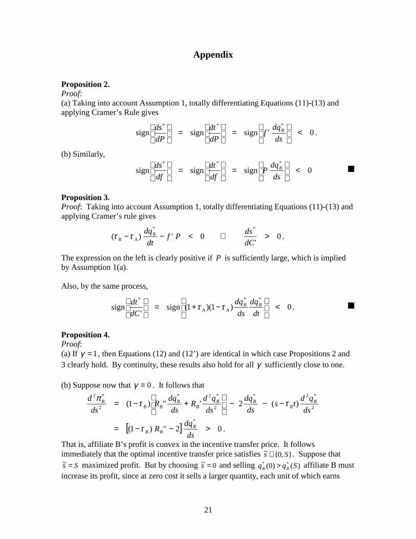
Proposition 2. Proof: (a) Taking into account Assumption 1, totally differentiating Equations (11)-(13) and applying Cramer’s Rule gives

0signsignsign***

<

=

=

dsdq'f

dPdt

dPds B .

(b) Similarly,

0signsignsign***

<

=

=

dsdqP

dfdt

dfds B g

Proposition 3. Proof: Taking into account Assumption 1, totally differentiating Equations (11)-(13) and applying Cramer’s rule gives

00)(**

>⇒<−−'dC

dsP'fdt

dqBAB ττ .

The expression on the left is clearly positive if P is sufficiently large, which is implied by Assumption 1(a). Also, by the same process,

0)1)(1(signsign***

<

−+=

dtdq

dsdq

dC'dt BB

AA ττ . g

Proposition 4. Proof: (a) If 1=γ , then Equations (12) and (12’) are identical in which case Propositions 2 and 3 clearly hold. By continuity, these results also hold for all γ sufficiently close to one.

(b) Suppose now that 0=γ . It follows that

2

*2*

2

*2*

2

*2

)(2)1(ds

qdtsds

dqds

qd'Rds

dq''Rds

d BB

BBB

BBB

B ττπ−−−

+−=

[ ] 02)1(*

>−−=ds

dq''R BBBτ .

That is, affiliate B’s profit is convex in the incentive transfer price. It follows immediately that the optimal incentive transfer price satisfies },0{~ Ss ∈ . Suppose that

Ss =~ maximized profit. But by choosing 0~ =s and selling )()0( ** Sqq BB > affiliate B must increase its profit, since at zero cost it sells a larger quantity, each unit of which earns

22

positive marginal revenue. This contradicts the initial assertion that Ss =~ is optimal. Since s~ is characterized by a corner solution, it follows that 0'/~/~/~ === dCsddfsddPsd . Since we have established that s~ is effectively fixed for the purposes of comparative statics analysis (when 0=γ ), the expressions for dPdt /* , dfdt /* and '/* dCdt can be determined from analyzing Equations (11) and (13) in isolation. Applying Cramer’s rule, it is straightforward to show that Propositions 2 and 3, as they pertain to *t , continue to hold. By continuity, the results here also hold for all γ sufficiently close to zero. g Proposition 5. Proof: (a) Taking the approach of Propositions 2 and 3, totally differentiating Equations (11), (12’) and (13), applying Cramer’s Rule and evaluating at 1=γ gives

{ } 0])[1(signsign*

>−−=

''C''Rddt

AAτγ

.

0)2(sign~

sign*

>

−−=

P'fdt

dqd

sd BAB ττ

γ.

The second inequality follows directly from Assumption 1(a). By continuity, these results also hold for all γ sufficiently close to one. (b) Note that

γγγ ∂∂+=

*** ~ td

sddsdt

ddt .

Proposition 4(b) has already established that 0/~0 =⇒= γγ dsd . Also, it is clear from Equation (12) that 0/* =∂∂ γt . Thus, evaluated at 0=γ , 0/* =γddt . By continuity, these results also hold for all γ sufficiently close to zero. g Proposition 6. Proof: The arguments underlying Proposition 1 rely in no way upon the market structure, so certainly hold for market structures consistent with intrafirm trade satisfying the law of demand. Inspecting the proofs of Propositions 2 and 3, it is clear that these two results hold provided the market structures in countries A and B are consistent with 0/* >dtdqB and

0/* <dsdqB . Note also that it follows immediately from Equation (4) that, regardless of market structure, dsdqdtdq BBB // ** τ−= , implying that dtdqB /* and dsdqB /* are always of opposite sign. Finally, by definition, 0/* <dsdqB if affiliate B’s demand for affiliate A’s product satisfies the law of demand. g Proposition 7. Proof: Suppose that AA II µ=~ , where 0>µ . Consolidated after-tax profit is now

23

PatFqtqRqqCqR BBABBBBAAAASET )(][)()1()]()()[1( −−−−−++−−= τµττµτπ

Letting µττ AA =~ , consolidated after-tax profit can be rewritten as

.)(]~[)()1()]()()[~1( PatFqtqRqqCqR BBABBBBAAAASET −−−−−++−−= ττττπ

But this expression is identical to Equation (10) except that Aτ~ now replaces Aτ . This reflects the fact that the expressions for SE

Aπ and SEBπ remain essentially unchanged. It

follows immediately that, regardless of whether 1>µ or 1<µ , Propositions 2 and 3 remain unchanged. Similarly, in the absence of penalties the same argument applies to Proposition 1. g

24

References Amershi, A. and P. Cheng, 1990. Intrafirm resource allocation: The economics of transfer pricing and cost allocation in accounting, Contemporary Accounting Research, 7:61-99. Anctil, R. and S. Dutta, 1999. Transfer pricing, decision rights and divisional versus firm-wide performance evaluation, The Accounting Review, 74(1):87-104. Baldenius, T., N. Melamud and S. Reichelstein, 2002. Integrating managerial and tax objectives in transfer pricing, Working Paper, Columbia University. Baldenius, T., S. Reichelstein and S. Sahay, 1999. Negotiated versus cost-based transfer pricing, Review of Accounting Studies, 4(2): 67-91. Bucks, D. R. and M. Mazerof, 1993. The state solution to the federal government’s transfer pricing problem, National Tax Journal, 46(3): 385-92. Czechowicz, I. J., F. D. S. Choi and V. B. Bavishi, 1982. Assessing Foreign Subsidiary Performance Systems and Practices of Leading Multinational Companies. New York: Business International Corporation. Elitzur, R. and J. Mintz, 1996. Transfer pricing rules and corporate tax competition, Journal of Public Economics, 60: 401-22. Goolsbee, A. and E. Maydew, 2000. Coveting thy neighbor’s manufacturing: The dilemma of state income apportionment, Journal of Public Economics, 75:125-43. Gordon, R. and J. D. Wilson, 1986. An examination of multijurisdictional corporate income taxation under formula apportionment, Econometrica, 54(6): 1357-73. Halperin, R. M. and B. Srinidhi, 1991. U.S. income tax transfer-pricing rules and resource allocation: The case of decentralized multinational firms, The Accounting Review, 56(1):141-157. Harris, M., C. Kriebel and A. Raviv, 1982. Asymmetric information, incentives and intrafirm resource allocation, Management Science, 28:604-20. Haufler, A. and G. Schjelderup, 2000. Corporate tax systems and cross country profit shifting, Oxford Economic Papers, 52:306-25. Holmstrom, B. and J. Tirole, 1991. Transfer pricing and organizational form, Journal of Law, Economics and Organization, 7:201-28. Horngren, C., G. Foster and S. Datar, 1997. Cost Accounting: A Managerial Emphasis, Annotated Instructors Edition. 9 ed., Englewood Cliffs: Prentice-Hall.

25

Kant, C., 1990. Multinational firms and government revenues, Journal of Public Economics, 42:135-47. Kant, C., 1988. Endogenous transfer pricing and the effects of uncertain regulation, Journal of International Economics, 24:147-57. Musgrave, P., 1973. International tax base division and the multinational corporation, Public Finance, 27(4):394-411. Nielsen, S. B., P. R. Raimondos-Moller and G. Schjelderup, 2001. Formula apportionment and transfer pricing under oligopolistic competition. CESifo Working Paper No. 491.

OECD, 1995. Transfer pricing guidelines for multinational enterprises and tax administrations, Paris: OECD Publications Service. Samuelson, L., 1982. The multinational firm with arm’s length transfer pricing limits, Journal of International Economics, 13:365-74. Sansing, R., 1999. Relationship-specific investments and the transfer pricing paradox, Review of Accounting Studies, 4:119-34. Schjelderup, G. and L. Sorgard, 1997. Transfer Pricing as a Strategic Device for Decentralized Multinationals. International Tax and Public Finance, 4:277-90. Smith, M., 2002. Ex ante and ex post discretion over arm’s length transfer prices, The Accounting Review, 77:161-84. Vaysman, I., 1995. A Model of Negotiated Transfer Pricing, Working Paper, U.T. Austin. Vickers, J., 1985. Delegation and the theory of the firm, Economic Journal, 95:138-47. Williamson, O., 1985. The Economic Institutions of Capitalism, New York: Free Press.