Embed Size (px)
Citation preview

Kernel Inverse Regression for spatial random fields
Jean-Michel Loubes, Anne-Francoise Yao
To cite this version:
Jean-Michel Loubes, Anne-Francoise Yao. Kernel Inverse Regression for spatial random fields.2008. <hal-00347813>
HAL Id: hal-00347813
https://hal.archives-ouvertes.fr/hal-00347813
Submitted on 16 Dec 2008
HAL is a multi-disciplinary open accessarchive for the deposit and dissemination of sci-entific research documents, whether they are pub-lished or not. The documents may come fromteaching and research institutions in France orabroad, or from public or private research centers.
L’archive ouverte pluridisciplinaire HAL, estdestinee au depot et a la diffusion de documentsscientifiques de niveau recherche, publies ou non,emanant des etablissements d’enseignement et derecherche francais ou etrangers, des laboratoirespublics ou prives.

KERNEL INVERSE REGRESSION FOR SPATIAL RANDOM FIELDS.
JEAN-MICHEL LOUBES AND ANNE-FRANCOISE YAO §
Abstract. In this paper, we propose a dimension reduction model for spatially depen-
dent variables. Namely, we investigate an extension of the inverse regression method
under strong mixing condition. This method is based on estimation of the matrix of
covariance of the expectation of the explanatory given the dependent variable, called the
inverse regression. Then, we study, under strong mixing condition, the weak and strong
consistency of this estimate, using a kernel estimate of the inverse regression. We provide
the asymptotic behaviour of this estimate. A spatial predictor based on this dimension
reduction approach is also proposed. This latter appears as an alternative to the spatial
non-parametric predictor.
Keywords: Kernel estimator; Spatial regression; Random fields; Strong mixing coef-
ficient; Dimension reduction; Inverse Regression.
1. Introduction
Spatial statistics includes any techniques which study phenomenons observed on spatial
subset S of RN , N ≥ 2 (generally, N = 2 or N = 3). The set S can be discret, continuous
or the set of realization of a point process. Such techniques have various applications in
several domains such as soil science, geology, oceanography, econometrics, epidemiology,
forestry and many others (see for example [27], [11] or [18] for exposition, methods and
applications).
Most often, spatial data are dependents and any spatial model must be able to handle
this aspect. The novelty of this dependency unlike the time-dependency, is the lack of
order relation. In fact, notions of past, present and futur does not exist in space and this
property gives great flexibility in spatial modelling.
In the case of spatial regression that interests us, there is an abundant literature on
parametric models. We refer for example to the spatial regression models with correlated
errors often used in economics (see e.g. Anselin and Florax [2], Anselin and Bera [1], Song
and Lee [29]) or to the spatial Generalized Linear Model (GLM) study in Diggle et al.
[14] and Zhang [36]. Recall also the spatial Poisson regression methods which have been
proposed for epidemiological data (see for example Diggle [13] or Diggle et al [14]).
§ Corresponding author : University Aix-Marseille 2, Campus de Luminy, case 901, 13288 Marseille cedex09. [email protected]. University Toulouse 3, Institut de Mathematiques de Toulouse.
1

englishKERNEL INVERSE REGRESSION FOR SPATIAL RANDOM FIELDS. 2
Unlike the parametric case, the spatial regression on nonparametric setting have been
studied by a few paper: quote for example Biau and Cadre [5], Lu and Chen [25], Hallin
et al. [19], Carbon et al. [9], Tran and Yakowitz [32] and Dabo-Niang and Yao [12].
Their results show that, as in the i.i.d. case, the spatial nonparametric estimator of the
regression function is penalized by the dimension of the regressor. This is the spatial
counterpart of the well-known problem called “the curse of dimensionality”. Recall that
dimension reduction methods are classically used to overcome this issue. Observing an
i.i.d. sample Zi = (Xi, Yi) the aim is to estimate the regression function m(x) = E(Y |X =
x). In the dimension reduction framework, one assumes that there exist Φ an orthonormal
matrix d ×D, with D as small as possible, and g : RD → R, an unknown function such
that the function m(.) can be written as
(1.1) m(x) = g(Φ .X).
Model (1.1) conveys the idea that “less information on X” , Φ .X; provides as much infor-
mation on m(.) as X. The function g is the regression function of Y given the D dimen-
sional vector Φ.X. Estimating the matrix Φ and then the function g (by nonparametric
methods) provides an estimator which converges faster than the initial nonparametric
estimator. The operator Φ is unique under orthogonal transformation. An estimation of
this latter is done through an estimation of his range Im(ΦT ) (where ΦT is the transpose
of Φ) called Effective Dimensional Reduction space (EDR).
Various methods for dimension reduction exist in the literature for i.i.d observations.
For example we refer to the multiple linear regression, the generalized linear model (GLM)
in [8], the additive models (see e.g. Hastie and Tibshirani [21]) deal with methods based
on estimation of the gradient of the regression function m(.) developped in for example
in [22] or [35].
In this paper, we focus on the inverse regression method, proposed by Li [24]: if X is
such that for all vector b in Rd, there exists a vector B of R
D such that E(bTX|Φ.X) =
BT (Φ.X) (this latter condition is satisfied as soon as X is elliptically distributed), then,
if Σ denotes the variance of X, the space Im(Σ−1var(E(X|Y )) is included into the EDR
space. Moreover, the two spaces coincide if the matrix Σ−1var(E(X|Y )) is of full rank.
Hence, the estimation of the EDR space is essentially based on the estimation of the
covariance matrix of the inverse regression E(X|Y ) and Σ which is estimated by using a
classical empirical estimator. In his initial version, Li suggested an estimator based on the
regressogram estimate of E(X|Y ) but drawbacks of the regressogram lead other authors
to suggest alternatives based on the nonparametric estimation of EX|Y , see for instance
[23] or [37] which enable to recover the optimal rate of convergence in√n.

englishKERNEL INVERSE REGRESSION FOR SPATIAL RANDOM FIELDS. 3
This work is motivated by the fact that to our knowledge, there is no inverse regression
method estimation for spatially dependent data under strong mixing condition. Note
however that a dimension reduction method for supervised motion segmentation based
on spatial-frequential analysis called Dynamic Sliced Inverse Regression (DSIR) has been
proposed by Wu and Lu [34]. We propose here a spatial counterpart of the estimating
method of [37] which uses kernel estimation of EX|Y . Other methods based on other
spatial estimators of EX|Y will be the subject of futher investigation.
As any spatial model, a spatial dimension reduction model must take into account
spatial dependency. In this work, we focus on an estimation on model (1.1) for spatial
dependent data under strong mixing conditions. The spatial kernel regression estimation
of EX|Y being studied in [5, 10, 9].
An important problem in spatial modelling is that of spatial prediction. The aim being
reconstruction of a random field over some domain from a set of observed values. It is
such a problem that interest us in the last part of this paper. More precisely, we will use
the properties of the inverse regression method to build a dimension reduction predictor
which corresponds to the nonparametric predictor of [5]. It is an interesting alternative to
parametric predictor methods such as the krigging methods (see e.g. [33], [11]) or spatial
autoregressive model (see for example [11]) since it does not requires any underlying
model. It only requires the knowledge of the number of the neighbors. We will see that
the property of the inverse regression method provides a way of estimating this number.
This paper falls into the following parts. Section 2 provides some notations and as-
sumptions on the spatial process, as well as some preliminar results on U-statistics. The
estimation method and the consistency results are presented in Section 3. Section 4 uses
this estimate to forecast a spatial process. Section 5 is devoted to Conclusion. Proofs and
the technical lemmas are gathered in Section 6.
2. General setting and preliminary Results
2.1. Notations and assumptions. Throughout all the paper, we will use the following
notations.
For all b ∈ Rd , b(j) will denote the jth component of the vector b;
a point in bold i = (i1, ..., iN) ∈ n ∈ (N∗)N will be referred to as a site, we will set
1N = ( 1, ..., 1︸ ︷︷ ︸N times
); if n = (n1, ..., nN ), we will set n = n1 × ... × nN and write n → +∞ if
mini=1,...,N ni → +∞ and ni
nk< C for some constant C > 0.
The symbol ‖.‖ will denote any norm over Rd , ‖u‖∞ = supx |u(x)| for some function u

englishKERNEL INVERSE REGRESSION FOR SPATIAL RANDOM FIELDS. 4
and C an arbitrary positive constant. If A is a set, let 1A(x) =
1 if x ∈ A
0 otherwise.
The notation Wn = Op(Vn) (respectively Wn = Oa.s(Vn)) means that Wn = VnSn for a
sequence Sn, which is bounded in probability (respectively almost surely).
We are interested in some Rd ×R-valued stationary and measurable random field Zi =
(Xi, Yi), i ∈ (N∗)N , (N, d ≥ 1) defined on a probability space (Ω, A,P). Without loss
of generality, we consider estimations based on observations of the process (Zi, i ∈ ZN )
on some rectangular set In =i = (i1, ..., iN) ∈ Z
N , 1 ≤ ik ≤ nk, k = 1, ..., N
for all n ∈(N∗)N .
Assume that the Zi’s have the same distribution as (X, Y ) which is such that:
• the variable Y has a density f .
• ∀j = 1, ..., d each component X(j) of X, is such that the pair (X(j), Y ) admits an
unknown density fX(j),Y with respect to Lebesgue measure λ over R2 and each
X(j) is integrable.
2.2. Spatial dependency.
As mentionned above, our model as any spatial model must take into account spatial
dependence between values at differents locations. Of course, we could consider that there
is a global linear relationships between locations as it is generally done in spatial linear
modeling, we prefer to use a nonlinear spatial dependency measure. Actually, in many
circumstances the spatial dependency is not necessarly linear (see [3]). It is, for example,
the classical case where one deals with the spatial pattern of extreme events such as in the
economic analysis of poverty, in the environmental science,... Then, it is more appropriate
to use a nonlinear spatial dependency measure such as positive dependency (see [3]) or
strong mixing coefficients concept (see Tran [31]). In our case, we will measure the
spatial dependency of the concerned process by means of α−mixing and local dependency
measure.
2.2.1. Mixing condition :
The field (Zi) is said to satisfy a mixing condition if:
• there exists a function X : R+ → R
+ with X (t) ↓ 0 as t→ ∞, such that whenever
S, S ′ ⊂ (N∗)N ,
α(B(S),B(S ′)) = supA∈B(S), B∈B(S′)
|P (B ∩ C) − P (B)P (C)|
≤ ψ(CardS, CardS ′)X (dist(S, S ′))(2.1)

englishKERNEL INVERSE REGRESSION FOR SPATIAL RANDOM FIELDS. 5
where B(S)(resp. B(S ′)) denotes the Borel σ−fields generated by (Zi, i ∈ S) (resp.
(Zi, i ∈ S ′)), CardS (resp. CardS ′) the cardinality of S(resp. S ′), dist(S, S ′) the
Euclidean distance between S and S ′, and ψ : N2 → R
+ is a symmetric positive
function nondecreasing in each variable. If ψ ≡ 1, then Zi is called strong mixing.
It is this latter case which will be tackled in this paper and for all v ≥ 0, we have
α (v) = supi, j∈RN ,‖i−j‖=v
α (σ (Zi) , σ (Zj)) ≤ X (v).
• The process is said to be Geometrically Strong Mixing (GSM) if there exists a
non-negative constant ρ ∈ [0, 1[ such that for all u > 0, α(u) ≤ Cρu .
Remark. A lot of published results have shown that the mixing condition (2.1) is satis-
fied by many time series and spatial random processes (see e.g. Tran [31], Guyon [18],
Rosenblatt [28], Doukhan [15]). Moreover, the results presented in this paper could be
extended under additional technical assumptions to the case, often considered in the lit-
erature, where ψ satisfies:
ψ(i, j) ≤ c min(i, j), ∀ i, j ∈ N,
for some constant c > 0.
In the following, we will consider the case where α(u) ≤ Cu−θ, for some θ > 0. But,
the results can be easly extend to the GSM case.
2.2.2. Local dependency measure.
In order to obtain the same rate of convergence as in the i.i.d case, one requires an
other dependency measure, called a local dependency measure. Assume that
• For ℓ = 1, ..., d, there exits a constant ∆ > 0 such that the pairs (X(ℓ)i , Xj) and
((X(ℓ)i , Yi), (X
(ℓ)j , Yj)) admit densities fi,j and gi,j, as soon as dist(i, j) > ∆, such
that
|fi, j (x, y) − f (x) f (y) | ≤ C, ∀x, y ∈ R
|gi, j (u, v) − g (u) g (v) | ≤ C, ∀u, v ∈ R2
for some constant C ≥ 0.
Remark. The link between the two dependency measures can be found in Bosq [7].
Note that if the second measure (as is name point out) is used to control the local
dependence, the first one is a kind of “asymptotic dependency” control.

englishKERNEL INVERSE REGRESSION FOR SPATIAL RANDOM FIELDS. 6
2.3. Results on U-statistics.
Let (Xn, n ≥ 1) be a sequence of real-valued random variables with the same distribu-
tion as F . Let the functional:
Θ(F ) =
∫
Rm
h(x1, x2, ..., xm)dF (x1)...dF (xm),
where m ∈ N, h(.) is some measurable function, called the kernel and F is a distribu-
tion function from some given set of distribution function. Without loss of generality,
we can assume that h(.) is invariable by permutation. Otherwise, the transformation1
m!
∑1≤i1 6=i2 6=... 6=im≤n h(xi1 , ..., xim) will provide a symmetric kernel.
A U−statistic with kernel h(.) of degree m based on the sample (Xi, 1 ≤ i ≤ n) is a
statistic defined by:
Un =(n−m)!
n!
∑
1≤i1 6=i2 6=... 6=im≤n
h(Xi1 , ..., Xim)
It is said to be an m−order U−statistic. Let h1(x1) =∫
Rm−1 h(x1, x2, ..., xm)∏m
j=2 dF (xj).
The next Lemma is a consequence of Lemma 2.6 of Sun & Chian [30].
Lemma 2.1. Let (Xn, n ≥ 1) be a stationary sequence of strongly mixing random
variables. If there exists a positive number δ and δ′ (0 < δ′ < δ) verifying γ = 6(δ−δ′)(4+δ)(2+δ′)
>
1 such that
(2.2) ||h(X1, ..., Xm)||4+δ <∞,
(2.3)
∫
Rm
|h(x1, ..., xm)|4+δm∏
j=1
dF (xj) <∞,
and α(n) = O(n−3(4+δ′)/(2+δ′)) . Then,
Un = Θ(F ) +2
n
n∑
i=1
(h1(Xi) − Θ(F )) + Op(1
n).
To give strong consistency results, we need the following law of the iterated logarithm
of U-statistics:
Lemma 2.2. (Sun & Chian, [30]) Under the same conditions of the previous lemma, we
have
Un − Θ(F ) =2
n
n∑
i=1
(h1(Xi) − Θ(F )) + Oa.s
(√log log n
n
)
.
Remark 2.3.

englishKERNEL INVERSE REGRESSION FOR SPATIAL RANDOM FIELDS. 7
• In the following, we are dealing with a kernel h(.) = K( .hn
) which depends on
n. Actually, it is a classical approach to use U−statistics result to get some
assymptotic results of kernel estimators, in the i.i.d case, we refer for example
Hardle and Stoker [20]. In fact, the dependence of hn on n does not influence the
asymptotical results presented here.
3. Estimation of the covariance of Inverse Regression Estimator
We suppose that one deals with a random field (Zi, i ∈ ZN ) which, corresponds, in the
spatial regression case, to observations of the form Zi = (Xi, Yi), i ∈ ZN , (N ≥ 1) at
different locations of a subset of RN , N ≥ 1 with some dependency structure. Here, we
are particularly interested with the case where the locations take place in lattices of RN .
The general continuous case will be the subject of a forthcoming work.
We deal with the estimation of the matrix Σe = varE(X|Y ) based on the observations
of the process: (Zi, i ∈ In) ; n ∈ (N∗)N . In order to ensure the existence of the matrix
Σ = varX and Σe = varE(X|Y ), we assume that E||X||4 < ∞. For sake of simplicity
we will consider centered process so EX = 0.
To estimate model (1.1), as previously mentioned, one needs to estimate the matrix
Σ−1Σe. On the one hand, we can estimate the variance matrix Σ by the empirical spatial
estimator, whose consistency will be easily obtained. On the other hand, the estimation
of the matrix Σe is delicate since it requires the study of the consistency of a suitable
estimator of the (inverse) regression function of X given Y :
r(y) =
ϕ(y)f(y)
if f(y) 6= 0;
EY if f(y) = 0where ϕ(y) =
(∫
R
x(i)fX(i),Y (x(i), y)dx, 1 ≤ i ≤ d
), y ∈ R.
An estimator of the inverse regression function r(.), based on (Zi, i ∈ In) is given by
rn(y) =
ϕn(y)fn(y)
if fn(y) 6= 0,1n
∑i∈In
Yi if fn(y) = 0,
with for all y ∈ R,
fn(y) =1
nhn
∑
i∈In
K
(y − Yi
hn
)
ϕn(y) =1
nhn
∑
i∈In
XiK
(y − Yi
hn
),
where fn is a kernel estimator of the density, K : Rd → R is a bounded integrable kernel
such that∫K (x) dx = 1 and the bandwidth hn ≥ 0 is such that limn→+∞ hn = 0.

englishKERNEL INVERSE REGRESSION FOR SPATIAL RANDOM FIELDS. 8
The consistency of the estimators fn and rn has been studied by Carbon et al [10]. To
prevent small-valued density observations y, we consider the following density estimator:
fe,n(y) = max(en, fn(y))
where (en) is a real-valued sequence such that limn→∞ en = 0. Then, we consider the
corresponding estimator of r
re,n(y) =ϕn(y)
fe,n(y).
Finally, for X = 1n
∑i∈In
Xi we consider the estimator of Σe:
Σe,n =1
n
∑re,n(Yi) re,n(Yi)
T −XXT.
We aim at proving the consistency of the empirical variance associated to this estimator.
Remark. Here, we consider as estimator of the density f , fe,n = max(en, fn), to avoid
small values. There are other alternatives such as fe,n = fn+en or fe,n = max(fn−en), 0.
3.1. Weak consistency. In the following, for a fixed η > 0 and a random variable Z
in Rd, we will use the notation ‖Z‖η = E(||Z||η)1/η.
In this section, we will make the following technical assumptions
(3.1)
∥∥∥∥r(Y )
f(Y )
∥∥∥∥4+δ1
<∞, for some δ1 > 0
and
(3.2)
∥∥∥∥r(Y )
f(Y )1f(Y )≤en
∥∥∥∥2
= O(
1
n1+δ2
). for some 1 > δ > 0.
These assumptions are the spatial counterparts of respectively ‖r(Y )‖4+δ < ∞ and∥∥r(Y ) 1f(Y )≤en
∥∥2
= O(
1
n14+δ
)needed in the i.i.d case.
We also assume some regularity conditions on the functions: K(.), f(.) and r(.):
• The kernel function K(.) : R → R+ is a k−order kernel with compact support
and satisfying a Lipschitz condition |K (x) −K (y)| ≤ C|x− y|• f(.) and r(.) are functions of Ck(R) (k ≥ 2) such that supy |f (k)(y)| < C1 and
supy ||ϕ(k)(y)|| < C2 for some constants C1 and C2,
Set Ψn = hkn +
√log n√nhn
.
Theorem 3.1. Assume that α(t) ≤ Ct−θ, t > 0, θ > 2N and C > 0. If E(||X||) <∞ and
ψ(.) = E(||X||2|Y = .) is continuous. Then for a choice of hn such that nh3n(log n)−1 → 0
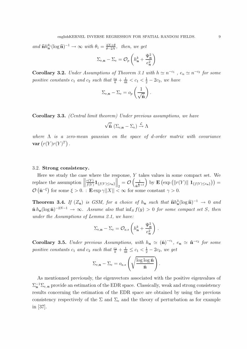
englishKERNEL INVERSE REGRESSION FOR SPATIAL RANDOM FIELDS. 9
and nhθ1n (log n)−1 → ∞ with θ1 = 4N+θ
θ−2N, then, we get
Σe,n − Σe = Op
(hk
n +Ψ2
n
e2n
)
Corollary 3.2. Under Assumptions of Theorem 3.1 with h ≃ n−c1 , en ≃ n−c2 for some
positive constants c1 and c2 such that c2k
+ 14k< c1 <
12− 2c2, we have
Σe,n − Σe = op
(1√n
).
Corollary 3.3. (Central limit theorem) Under previous assumptions, we have√
n (Σe,n − Σe)L→ Λ
where Λ is a zero-mean gaussian on the space of d-order matrix with covariance
var(r(Y )r(Y )T
).
3.2. Strong consistency.
Here we study the case where the response, Y takes values in some compact set. We
replace the assumption∥∥∥ r(Y )
f(Y )1f(Y )≤en
∥∥∥2
= O(
1
n12+δ
)by E
(exp
(‖r(Y )‖ 1f(Y )≤en
))=
O(n−ξ)
for some ξ > 0. : E exp γ||X|| <∞ for some constant γ > 0.
Theorem 3.4. If (Zu) is GSM, for a choice of hn such that nh3n(log n)−1 → 0 and
nhn(log n)−2N−1 → ∞. Assume also that infS f(y) > 0 for some compact set S, then
under the Assumptions of Lemma 2.1, we have:
Σe,n − Σe = Oa.s
(hk
n +Ψ2
n
e2n
).
Corollary 3.5. Under previous Assumptions, with hn ≃ (n)−c1, en ≃ n−c2 for some
positive constants c1 and c2 such that c2k
+ 14k
≤ c1 <12− 2c2, we get
Σe,n − Σe = oa.s
(√log log n
n
).
As mentionned previously, the eigenvectors associated with the positive eigenvalues of
Σ−1n Σe, n provide an estimation of the EDR space. Classically, weak and strong consistency
results concerning the estimation of the EDR space are obtained by using the previous
consistency respectively of the Σ and Σe and the theory of perturbation as for example
in [37].

englishKERNEL INVERSE REGRESSION FOR SPATIAL RANDOM FIELDS. 10
4. Spatial inverse methode for spatial prediction
4.1. Prediction of a spatial process.
Let (ξn, n ∈ (N∗)N ) be a R−valued strictly stationary random spatial process, assumed
to be observed over a subset On ⊂ In (In is a rectangular region as previously defined
for some n ∈ (N∗)N). Our aim is to predict the square integrable value, ξi0, at a given
site i0 ∈ In − On. In practice, one expects that ξi0 only depends on the values of the
process on a bounded vicinity set (as small as possible) Vi0 ⊂ On; i.e that the process (ξi)
is (at least locally) a Markov Random Field (MRF) according to some system of vicinity.
Here, we will assume (without loss of generality) that the set of vicinity (Vj, j ∈ (N∗)N)
is defined by Vj of the form j + V (call vicinity prediction in Biau and Cadre [5]). Then
it is well known that the minimum mean-square error of prediction of ξi0 given the data
in Vi0 is
E(ξi0|ξi, i ∈ Vi0)
and we can consider as predictor any d−dimensional vector (where d is the cardinal of V)
of elements of Vi0 concatenated and ordered according to some order. Here, we choose the
vector of values of (ξn) which correspond to the d−nearest neighbors: for each i ∈ ZN ,
we consider that the predictor is the vector ξdi = (ξi(k); 1 ≤ k ≤ d) where i(k) is the k−th
nearest neighbor of i. Then, our problem of prediction amounts to estimate :
m(x) = E(ξi0|ξdi0
= x).
For this purpose we construct the associated process:
Zi = (Xi, Yi) = (ξdi , ξi), i ∈ Z
N
and we consider the estimation of m(.) based on the data (Zi,∈ On) and the model
(1.1). Note that the linear approximation of m(.) leads to linear predictors. The available
literature on such spatial linear models (we invite the reader think of the kriging method
or spatial auto-regressive method) is relatively abundant, see for example, Guyon [18],
Anselin and Florax [2], Cressie [11], Wackernagel [33]. In fact, the linear predictor is the
optimal predictor (in mimimun mean square error meaning) when the random field under
study is Gaussian. Then, linear techniques for spatial predicition, give unsatisfactory
results when the the process is not Gaussian. In this latter case, other approaches such as
log-normal kriging or the trans-Gaussian kriging have been introduced. These methods
consist in transforming the original data into a Gaussian distributed data. But, such
methods lead to outliers which appear as an effect of the heavy-tailed densities of the data
and cannot be delete. Therefore, a specific consideration is needed. This can be done by
using, for example, a nonparametric model. That is what is proposed by Biau and Cadre

englishKERNEL INVERSE REGRESSION FOR SPATIAL RANDOM FIELDS. 11
[5] where a predictor based on kernel methods is developped. But, This latter (the kernel
nonparametric predictor) as all kernel estimator is submitted to the so-called dimension
curse and then is penalized by d (= card(V)), as highlighted in Section 1. Classically,
as in Section 1, one uses dimension reduction such as the inverse regression method, to
overcome this problem. We propose here an adaptation of the inverse regression method
to get a dimension reduction predictor based on model (1.1):
(4.1) ξi = g(Φ.ξdi ).
Remark 4.1.
(1) To estimate this model, we need to check the SIR condition in the context of
prediction i.e: X is such that for all vector b in Rd, there exists a vector B of
RD such that E(bTX|Φ.X) = BT (Φ.X), is verify if the process (ξi) is a spatial
elliptically distributed process such as Gaussian random field.
(2) In the time series forecasting problem, “inverse regression” property can be an
“handicap”, since then, one needs to estimate the expectation of the “future”
given the “past”. So, the process under study must be reversible. The flexibility
that provide spatial modelling overcome this default since as mentioned in the
introduction, the notion of past, present and future does not exist.
At this stage, one can use the method of estimation of the model (1.1) given in Section
1 to get a predictor. Unfortunately (as usually in prediction problem) d is unknown in
practice. So, we propose to estimate d by using the fact that we are dealing both with a
Markov property and inverse regression as follows.
4.2. Estimation of the number of neighbors necessary for prediction.
Note that we suppose that the underline process is a stationary Markov process with
respect to the d−neighbors system of neighborhood, so the variables ξi(k) and ξi are
independent as soon as k > d and
E(ξi(k)|ξi = y) = 0
(since (ξi) is a stationary zero mean process).
Futhermore since our estimator (of model (1.1)) is based on estimation of E(X|Y =
y) = E(ξdi |ξi = y) = (E(ξi(k)|ξi = y); 1 ≤ k ≤ d), that allows us to keep only the neighbors
ξi(k) for which E(ξi(k)|ξi = y) 6= 0. Then, an estimation of d is obtained by estimation of
argminkE(ξi(k)|ξi = y) = 0. We propose the following algorithm to get this estimator.

englishKERNEL INVERSE REGRESSION FOR SPATIAL RANDOM FIELDS. 12
Algorithm for estimation of d, the number of neighbors.
(1) Initialization: specify a parameter δ > 0 (small) and fix a site j0; set k = 1.
(2) compute r(k)n (y) =
∑
i∈On,Vj0⊂On
ξi(k) Khn (y−ξi)
∑
i∈On,Vj0⊂On
Khn(y−ξi)
, the kernel estimate of r(k)(y) =
E(X(k)|Y = y)
(3) if |(r(k)n (y)| > δ, then k = k+1 and continue with Step 2; otherwise terminate and
d = k.
Then, we can compute a predictor based on d = k:
4.3. The dimension reduction predictor.
To get the predictor, we suggest the following algorithm:
(1) compute
r∗n(y) =
∑
i∈On,Vi0⊂On
ξdi Khn
(y − ξi)
∑
i∈On,Vi0⊂On
Khn(y − ξi)
(2) compute
Σe,n =1
n
∑
i∈On,Vi0⊂On
r∗e,n(Yi) r∗e,n(Yi)
T −XXT.
(3) Do the principal component analisys of Σ−1n Σe,n both to get a basis of Im(Σ−1
n Σe,n)
and estimation of the D, the dimension of Im(Φ) as suggested in the next remark
(4) compute the predictor:
ξi0 = g∗n(Φ∗n.Xi0).
based on data (Zi, i ∈ On); where g∗n is the kernel estimate:
g∗n(x) =
∑
i∈On,Vi0⊂On
ξiKhn
(Φ∗
n(x− ξdi ))
∑
i∈On,Vi0⊂On
Khn
(Φ∗
n(x− ξdi )) ∀x ∈ R
d.
Remark 4.2.
(1) The problem of estimation of D in step (4) is a classical problem in dimension
reduction problems. Several ways exist in the literature. One can for example
use the eigenvalues representation of the matrix Σ−1n Σe, n, the measure of distance
between spaces as in Li [24] or the selection rule of Ferre [16].
englishKERNEL INVERSE REGRESSION FOR SPATIAL RANDOM FIELDS. 13
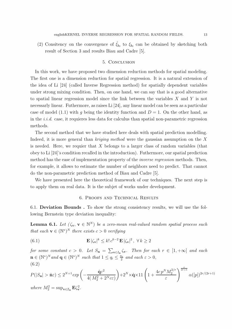
(2) Consitency on the convergence of ξi0 to ξi0 can be obtained by sketching both
result of Section 3 and results Biau and Cadre [5].
5. Conclusion
In this work, we have proposed two dimension reduction methods for spatial modeling.
The first one is a dimension reduction for spatial regression. It is a natural extension of
the idea of Li [24] (called Inverse Regression method) for spatially dependent variables
under strong mixing condition. Then, on one hand, we can say that is a good alternative
to spatial linear regression model since the link between the variables X and Y is not
necessarly linear. Futhermore, as raises Li [24], any linear model can be seen as a particular
case of model (1.1) with g being the identity function and D = 1. On the other hand, as
in the i.i.d. case, it requieres less data for calculus than spatial non-parametric regression
methods.
The second method that we have studied here deals with spatial prediction modelling.
Indeed, it is more general than kriging method were the gaussian assumption on the X
is needed. Here, we requier that X belongs to a larger class of random variables (that
obey to Li [24]’s condition recalled in the introduction). Futhermore, our spatial prediction
method has the ease of implementation property of the inverse regression methods. Then,
for example, it allows to estimate the number of neighbors need to predict. That cannot
do the non-parametric prediction method of Biau and Cadre [5].
We have presented here the theoretical framework of our techniques. The next step is
to apply them on real data. It is the subjet of works under development.
6. Proofs and Technical Results
6.1. Deviation Bounds . To show the strong consistency results, we will use the fol-
lowing Bernstein type deviation inequality:
Lemma 6.1. Let ( ζv, v ∈ NN) be a zero-mean real-valued random spatial process such
that each v ∈ (N∗)N there exists c > 0 verifying
(6.1) E |ζv|k ≤ k! ck−2 E |ζv|2 , ∀ k ≥ 2
for some constant c > 0. Let Sn =∑
v∈Inζv. Then for each r ∈ [1,+∞] and each
n ∈ (N∗)Nand q ∈ (N∗)N such that 1 ≤ qi ≤ ni
2and each ε > 0,
(6.2)
P (|Sn| > nε) ≤ 2N+1exp
(− qε2
4(M22 + 2Ncε)
)+2N×q×11
(1 +
4c pNM2/r2
ε
) r2r+1
α([p])2r/(2r+1)
where M22 = supv∈In
Eζ2v.

englishKERNEL INVERSE REGRESSION FOR SPATIAL RANDOM FIELDS. 14
Remark 6.2. Actually, this result is an extension of Lemma 3.2 of Dabo-Niang and Yao [12]
for bounded processes. This extension is necessary since in the problem of our interessed,
assuming the boundness of the processes amounts to assume that the Xi’s are bounded. It
is a restrictive condition which (generally) is incompatible with the cornerstone condition
of the inverse regression (if X is elliptically distributed for example).
We will use the following lemma to get the weak consistency and a law of iterated of
the logarithm as well as for the matrix Σ (as we will see immediately) than for the matrix
Σe (see the proofs of results of Section 3).
Lemma 6.3. Let Xn, n ∈ NN be a zero-mean stationary spatial process sequence, of
strong mixing random variables.
(1) If E||X||2+δ < +∞ and∑α(n)
δ2+δ <∞, for some δ > 0. Then,
1
n
∑
i∈In
Xi = Op
(1
n
).
(2) If E||X||2+δ < +∞ and∑α(n)
δ2+δ <∞, for some δ > 0. Then,
√n(
1
n
∑
i∈In
Xi)/σ → N (0, 1)
with σ2 =∑
i∈ZN cov(Xk, Xi)
(3) If E exp γ||X|| < ∞ for some constant γ > 0, if for all u > 0 , α(u) ≤ aρ−u ,
0 < ρ < 1 or α(u) = C.u−θ, θ > N then,
1
n
∑
i∈In
Xi = oa.s
(√log log n
n
)
.
Remark 6.4.
• The first result is obtained by using covariance inequality for strong mixing pro-
cesses (see Bosq [7]). Actually, it suffices to enumerate the Xi ’s into an arbitrary
order and sketch the proof in Theorem 1.5 of Bosq [7].
• The law of the iterated of the logarithm holds by applying the previous Lemma 6.1
with ε = η√
log log n
n, η > 0 and q =
[n
log log n
]+ 1.
6.2. Consistency of the inverse regression. In Section 3, we have seen that the results
are based on consistency results of the function r(.) which are presented now under some
regularity conditions on the functions: K(.), f(.) and r(.).
• The kernel function K(.) : R → R+ is a k−order kernel with compact support
and satisfying a Lipschitz condition |K (x) −K (y)| ≤ C|x− y|

englishKERNEL INVERSE REGRESSION FOR SPATIAL RANDOM FIELDS. 15
• f(.) and r(.) are functions of Ck(R) (k ≥ 2) such that supy |f (k)(y)| < C1 and
supy ||ϕ(k)(y)|| < C2 for some constants C1 and C2,
we have convergence result:
Lemma 6.5. Suppose α(t) ≤ Ct−θ, t > 0, θ > 2N and C > 0. If nh3n(log n)−1 → 0,
nhθ1n (log n)−1 → ∞ with θ1 = 4N+θ
θ−2N, then
(1) (see, [10])
(6.3) supy∈R|fn(y) − f(y)| = Op (Ψn ) .
(2) Furthermore, if E(||X||) <∞ and ψ(.) = E(||X||2|Y = .) is continuous, then
(6.4) supy∈R||ϕn(y) − ϕ(y)|| = Op (Ψn) .
Remark 6.6. Actually, only the result (6.3) is shown in Carbon et al [10] but the result
(6.4) is easily obtained by noting that for all ε > 0,
P(supy∈R||ϕn(y)−Eϕn(y)|| > ε) ≤ E||X||
an
+P(supy∈R||ϕn(y)−Eϕn(y)|| > ε, ∀i, ||Xi|| ≤ an)
with an = η (log n)1/4, η > 0.
Lemma 6.7. If (Zu) is GSM, nh3n(log n)−1 → 0 and nhn(log n)−2N−1 → ∞, then
(6.5) supy∈R|fn(y) − f(y)| = Oa.s (Ψn) .
Furthermore, if E (exp γ ||X||) < ∞ for some γ > 0 and ψ(.) = E(||X||2|Y = .) is
continuous, then
(6.6) supy∈R||ϕn(y) − ϕ(y)|| = Oa.s (Ψn) .
Remark. The equality (6.5) is due to Carbon et al [10]. The proof of the equality (6.6) is
obtained applying Lemma 6.1 and sketching the proofs of Theorem 3.1 and 3.3 of Carbon
et al [10]. Then it is omitted.
We will need the following lemma and the spatial block decomposition:
Lemma 6.8. (Bradley’s Lemma in Bosq [6])
Let (X, Y ) be an Rd × R−valued random vector such that Y ∈ Lr(P ) for some r ∈
[1,+∞]. Let c be a real number such that ||Y + c||r > 0 and ξ ∈ (0, ||Y + c||r]. Then there
exists a random variable Y ∗ such that:
(1) PY ∗ = PY and Y ∗ is independent of X,
(2) P (|Y ∗ − Y | > ξ) ≤ 11 (ξ−1||Y + c||r)r/(2r+1) × [α (σ(X), σ(Y ))]2r/(2r+1).

englishKERNEL INVERSE REGRESSION FOR SPATIAL RANDOM FIELDS. 16
Spatial block decomposition.
Let Yu = ζv=([ui]+1, 1≤i≤N), u ∈ RN . The following spatial blocking idea here is that of
Tran [31] and Politis and Romano [26].
Let ∆i =∫ i1(i1−1)
...∫ iN(iN−1)
Yudu . Then,
Sn =
∫ n1
0
...
∫ nN
0
Yudu =∑
1 ≤ ik ≤ nk
k = 1, ...N
∆i.
So, Sn is the sum of 2NPN q1 × q2 ×· · ·× qN terms ∆i. And each of them is an integral
of Yu over a cubic block of side p. Let consider the classical block decomposition:
U(1,n, j) =
(2ji+1)p∑
ki=2jip+1, 1≤i≤N
∆k,
U(2,n, j) =
(2ji+1)p∑
ki=2jip+1, 1≤i≤N−1
2(jN+1)p∑
kN=(2jN+1)p+1
∆k,
U(3,n, x, j) =
(2ji+1)p∑
ki=2jip+1, 1≤i≤N−2
2(jN−1+1)p∑
kN−1=(2jN−1+1)p+1
(2jN+1)p∑
kN=2jN p+1
∆k,
U(4,n, j) =
(2ji+1)p∑
ki=2jip+1, 1≤i≤N−2
2(jN−1+1)p∑
kN−1=(2jN−1+1)p+1
2(jN+1)p∑
kN=(2jN+1)p+1
∆k,
and so on. Note that
U(2N−1,n, j) =
2(ji+1)p∑
ki=(2ji+1)p+1, 1≤i≤N−1
(2jN+1)p∑
kN=2jN p+1
∆k.
Finally,
U(2N ,n, j) =
2(ji+1)p∑
ki=(2ji+1)p+1, 1≤i≤N
∆k.
So,
(6.7) Sn =
2N∑
i=1
T (n, i),
with T (n, i) =∑ql−1
jl=0, l=1,...,N U(i,n, j).
If ni 6= 2pti, i = 1, ..., N , for all set of integers t1, ..., tN , then a term, say T(n, 2N + 1
)
containing all the ∆k’s at the end, and not included in the blocks above, can be added

englishKERNEL INVERSE REGRESSION FOR SPATIAL RANDOM FIELDS. 17
(see Tran [31] or Biau and Cadre [4]). This extra term does not change the result of
previous proof.
Proof of Lemma 6.1.
Using (6.7) it suffices to show that
(6.8)
P
(|T (n, i)| > nε
2N
)≤ 2 exp
(− ε2
4v2(q)q
)+q×11
(1 +
4C pNM2/r2
ε
)r/(2r+1)
α([p])2r/(2r+1)
for each 1 ≤ i ≤ 2N .
Without loss of generality we will show (6.8) for i = 1. Now, we enumerate (as it is
often done in this case) in arbitrary way the q = q1 × q2 ×· · ·× qN terms U(1,n, j) of sum
of T (n, 1) that we call W1, ...,Wq. Note that the U(1,n, j) are measurable with respect
to the σ−field generated by Yu with u such that 2jip ≤ ui ≤ (2ji + 1)p, i = 1, ..., N .
These sets of sites are separated by a distance at least p and since for all m = 1, ..., q
there exists a j(m) such that Wm = U(1,n, j(m)) which have the same distribution as
W ∗m ,
E|Wm|r = E|W ∗m|r = E
∣∣∣∣∣
∫ (2j1(m)+1)p
2j1(m)p
...
∫ (2jN (m)+1)p
2jN (m)p
Yudu
∣∣∣∣∣
r
, r ∈ [1, +∞].
Noting that
∫ (2jk(m)+1)p
2jk(m)p
Yu du =
∫ [2jk(m)p]+1
2jk(m)p
Yu du +
[(2jk(m)+1)p]∑
vk=[2jk(m)p]+2
ζv +
∫ 2jk(m)+1)p
[(2jk(m)+1)p]
Yu du
= ([2jk(m)p] + 1 − 2jk(m)p) ζ(v, vk=[2jk(m)p]+1) +
[(2jk(m)+1)p]∑
vk=[2jk(m)p]+2
ζv
+((2jk(m) + 1)p− [(2jk(m) + 1)p]) ζ(v, vk=[(2jk(m)+1)p]+1)
=
[(2jk(m)+1)p]+1∑
vk=[2jk(m)p]+1
w(j,v)k ζv
and |w(j,v)k| ≤ 1 ∀k = 1, ..., N , we have by using Minkovski’s inequality and 6.1 one get
(6.9) E
∣∣∣∣Wm
pN
∣∣∣∣r
≤ cr−2r!M22 , ∀r ≥ 2.

englishKERNEL INVERSE REGRESSION FOR SPATIAL RANDOM FIELDS. 18
Then, using recursively the version of Bradley’s lemma gives in Lemma 6.8 we define
independent random variables W ∗1 , ...,W
∗q such that for all r ∈ [1,+∞] and for all m =
1, ..., q, W ∗m has the same distribution with Wm and setting ωr
r = prNcr−2M22 , we have:
P (|Wm −W ∗m| > ξ) ≤ 11
( ||Wm + ωr||rξ
)r/(2r+1)
α([p])2r/(2r+1),
where, c = δωrp and ξ = min(
nε2N+1q
, (δ − 1)ωrpN)
= min(
εpN
2, (δ − 1)ωrp
N)
for some
δ > 1 specified below. Note that for each m,
||Wm + c||r ≥ c− ||Wm||r ≥ (δ − 1)ωrpN > 0
so that 0 < ξ < ||Wm + c||r as required in Lemma 6.8.
Then, if δ = 1 + ε2ωr
,
P (|Wm −W ∗m| > ξ) ≤ 11
(1 +
4ωr
ε
)r/(2r+1)
α([p])2r/(2r+1)
and
P
(q∑
m=1
|Wm −W ∗m| >
nε
2N+1
)≤ q × 11
(1 +
4ωr
ε
)r/(2r+1)
α([p])2r/(2r+1).
Now, note that Inequality (6.9) also leads (by Bernstein’s inequality) to :
P
(∣∣∣∣∣
q∑
m=1
W ∗m
∣∣∣∣∣ >nε
2N+1
)≤ 2 exp
(−
(nε
2N+1
)2
4∑q
m=1 EW 2m + cnpN
2N+1 ε
)
Thus
P (|T (n, 1)| > nε2N ) ≤ 2exp
(− qε2
4( M22 +2N cε)
)+ q × 11
(1 +
4c pNM2/r2
ε
)r/(2r+1)
α([p])2r/(2r+1)
Then, since q = q1 × ... × qN and n = 2NpN q, we get inequality (6.8) the proof is
completed by noting that P (|Sn| > nε) ≤ 2NP (|T (n, i)| > nε2N ).
6.3. Proof of the Theorem 3.1. We will prove the desired result on Σe, n − Σe using
an intermediate matrix
Σe,n =1
n
∑
i∈In
r(Yi)r(Yi)T .
Start with the following decomposition
Σe,n − Σe = Σe, n − Σe,n + Σe,n − Σe.
We first show that:
(6.10) Σe, n − Σe, n = Op
(1
n12+δ
+Ψ2
n
e2n
).

englishKERNEL INVERSE REGRESSION FOR SPATIAL RANDOM FIELDS. 19
To this aim, we set :
(6.11) Σe, n − Σe,n = Sn, 1 + Sn, 2 + Sn, 3
with
Sn,1 =1
n
∑
i∈In
(ren(Yi) − r(Yi)) (ren(Yi) − r(Yi))T ,
Sn, 2 =1
n
∑
i∈In
r(Yi) (ren(Yi) − r(Yi))T
and
Sn, 3 =1
n
∑
i∈In
(ren(Yi) − r(Yi)) r(Yi)T .
Note that STn, 3 = Sn, 2, hence we only need to control the rate of convergence of the first
two terms Sn, 1 and Sn, 2
We will successively prove that
Sn,1 = Op
(Ψ2
n
e2n
),
and
Sn,2 = Op
(Ψ2
n
e2n+ hk
n
)
this latter will immediately implies that
Sn,3 = Op
(Ψ2
n
e2n+ hk
n
).
• Control on Sn, 1
Since for each y ∈ R :
(6.12) ren(y) − r(y) =r(y)
fen(y)(f(y) − fen(y)) +
1
fen(y)(ϕn(y) − ϕ(y))
and
(6.13) f(y) − fen(y) = f(y) − fn(y) + (fn(y) − en)1fn(y)<en,
for each i ∈ (N∗)N
‖ren(Yi) − r(Yi)‖ ≤ ‖r(Yi)‖en
||fn − f ||∞ + 2 ‖r(Yi)‖1fn(Yi)<en +‖ϕn − ϕ‖∞
en.
and
‖ren(Yi) − r(Yi)‖2 ≤ 3
[‖r(Yi)‖2 ||fn − f ||2∞
e2n+ 4 ‖r(Yi)‖2
1fn(Yi)<en +||ϕn − ϕ||2∞
e2n
].

englishKERNEL INVERSE REGRESSION FOR SPATIAL RANDOM FIELDS. 20
Using the following inequality (see Ferre and Yao [17] for details):
(6.14) 1fn(Yi)<en ≤ 1f(Yi)<en +||fn − f ||2∞
e2n,
and by results on Lemmas 6.3 and 6.5, we have:
Sn,1 ≤C
n
∑
i∈In
‖r(Yi)‖21f(Yi)<en + Op
(Ψ2
n
e2n
), C > 0.
Now, noting that
1
n
∑
i∈In
‖r(Yi)‖21f(Yi)<en ≤ e2n
1
n
∑
i∈In
‖r(Yi)‖2
f(Yi)21f(Yi)<en,
we have (since E(
||r(Yi)||2f(Yi)2
1f(Yi)<en
)= O
(1
n1+δ
)by assumption):
(6.15)1
n
∑
i∈In
‖r(Yi)‖21f(Yi)<en = Op
(e2n
n1+δ
)
and
Sn,1 = Op
(e2n
n1+δ+
Ψ2n
e2n
)
because of Assumption E(
‖r(Y )‖2
f(Y )21f(Y )<en
)= O
(1
n1+δ
).
Now, since Ψn = hkn +
√log n
nhnand en
n1+δ2
≤ C√
log n
nhn(for n large and C > 0 an arbitrary
constante), we have:
(6.16) Sn,1 = Op
(Ψ2
n
e2n
).
• Control on Sn, 2 .
Noting that : 1fen
= 1f+ f−fen
fenf+ fen−fen
fen fen= 1
f+ f−en
fenf1f<en+
fen−fen
fenfen, with fen = maxf, en,
we have:
Sn, 2 =1
n
∑
i∈In
r(Yi)r(Yi)T
fen(Yi)(f(Yi) − fen(Yi)) +
r(Yi)
fen(Yi)(ϕn(Yi) − ϕ(Yi))
T
=1
n
∑
i∈In
r(Yi)r(Yi)T
f(Yi)(f(Yi) − fn(Yi)) +
r(Yi)
f(Yi)(ϕn(Yi) − ϕ(Yi))
T +Rn1 +Rn2 .
where
Rn1(Yi) = r(Yi)[r(Yi)
T (f(Yi) − fn(Yi)) + (ϕn(Yi) − ϕ(Yi))T]
(1
f(Yi)1f(Yi)<en +
fen(Yi) − fen(Yi)
fen(Yi)fen(Yi)
)

englishKERNEL INVERSE REGRESSION FOR SPATIAL RANDOM FIELDS. 21
and
Rn2 =r(Yi)r(Yi)
T
fen(Yi)(fn(Yi) − fen(Yi)) .
Futhermore :
• since for all y ∈ R we have 1fen (y)fen (y)
≤ 1e2n
and by several calculus we also have∣∣∣fen(y) − fen(y)∣∣∣ ≤ |f(y) − fn(y)| and then ||fen − fen||∞ ≤ ||fn − f ||∞ , we also
have one hand:
Rn1≤ 1
n
∑
i∈In
(||r(Yi)|| ||ϕn − ϕ||∞ + ||r(Yi)||2 ||fn − f ||∞
) ( 1
f(Yi)1f<en +
||fn − f ||∞e2n
)(6.17)
• on the other hand we have
Rn2 ≤ 1
n
∑
i∈In
||r(Yi)||2|fn(Yi) − en|fen(Yi)
1fn(Yi)<en
≤ 2
n
∑
i∈In
||r(Yi)||2 1fn(Yi)<en.
because for all y ∈ R , |fn(y) − fen(y)| = |fn(y) − en|1fn(y)<en ≤ 2en1fn(y)<en.
Then, it follows from (6.14 and 6.15) that:
Rn2 = Op
(e2n
n1+δ+
Ψ2n
e2n
)
as for Sn1 , we deduce:
Rn2 = Op
(Ψ2
n
e2n
)
Now, observious that,
1
n
∑
i∈In
||r(Yi)||2f(Yi)
1f(Yi)<en ≤ en1
n
∑
i∈In
||r(Yi)||2f(Yi)2
1f(Yi)<en,
we have (as previously):
(6.18)1
n
∑
i∈In
||r(Yi)||2f(Yi)
1f(Yi)<en = Op
( enn1+δ
).
Moreover, since E(
‖r(Y )‖2
f(Y )21f(Y )<en
)= O
(1
n1+δ
), we also have:
(6.19)1
n
∑
i∈In
||r(Yi)||f(Yi)
1f(Yi)<en = Op
(1
n1+δ2
)
So combining (6.17), (6.18) and (6.19), we get:
Rn1 = Op
(enΨn
n1+δ+
Ψn
n1+δ2
+Ψ2
n
e2n
)= Op
(Ψn
n1+δ2
+Ψ2
n
e2n
);

englishKERNEL INVERSE REGRESSION FOR SPATIAL RANDOM FIELDS. 22
and since en
n1+δ2
≤ C√
log n
nhn(for n large) we have:
Rn1 = Op
(Ψ2
n
e2n
).
Then,
Sn, 2 = S(1)n, 2 + S
(2)n, 2 + Op
(Ψ2
n
e2n
);
with
S(1)n, 2 =
1
n
∑
i=1
r(Yi)r(Yi)T
f(Yi)(fn(Yi) − f(Yi))
and
S(2)n, 2 =
1
n
∑
i=1
r(Yi)
f(Yi)(ϕn(Yi) − ϕ(Yi))
T .
To finish, we are going to show that
S(1)n, 2 = Op(h
kn +
1
nhn
)
S(2)n, 2 = Op(h
kn +
1
nhn
)
Note that:
S(1)n, 2 =
1
n
∑
i=1
τ(Yi) f(Yi) −1
hn
Vn
where τ(.) is a function defined by τ(y) = r(y) r(y)T
f(y)for y ∈ R and
Vn =1
n2
∑
i,j∈In
τ(Yi)Khn(Yi − Yj)
is a second-order Von Mises functional statistic which associated U-statistic is:
Un =1
2n(n− 1)
∑
i=1
∑
j 6=i
[τ(Yi) + τ(Yj)]Khn(Yi − Yj).
Since: Vn = Un + Op(1n),
S(1)n, 2 =
1
n
∑
i=1
τ(Yi) f(Yi) −1
hn
Un + Op
(1
nhn
).
We apply Lemma 2.1 with, m = 2, h(y1, y2) = [τ(y1) + τ(y2)]Khn(y1 − y2)
h1(y) =1
2[τ(y).f ∗Khn
(y) + (τ.f) ∗Khn(y)] ,
and
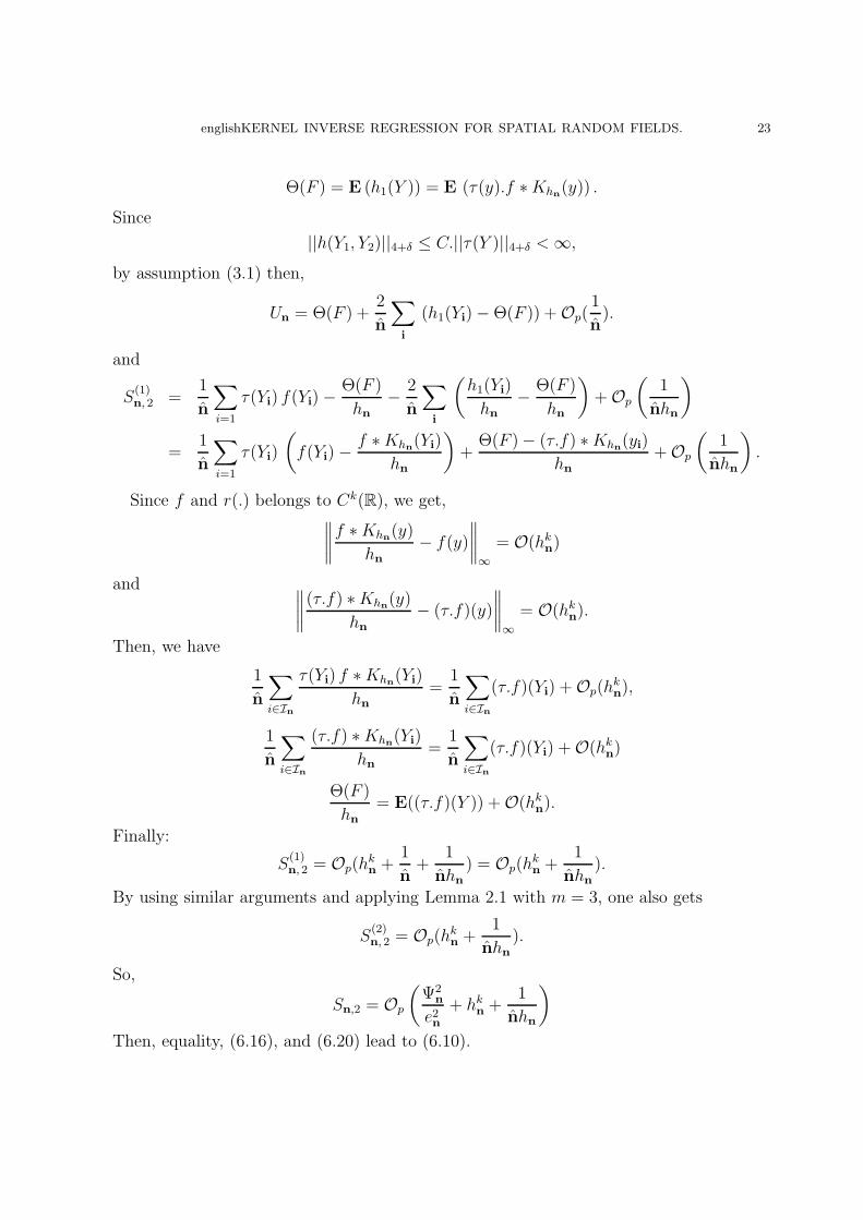
englishKERNEL INVERSE REGRESSION FOR SPATIAL RANDOM FIELDS. 23
Θ(F ) = E (h1(Y )) = E (τ(y).f ∗Khn(y)) .
Since
||h(Y1, Y2)||4+δ ≤ C.||τ(Y )||4+δ <∞,
by assumption (3.1) then,
Un = Θ(F ) +2
n
∑
i
(h1(Yi) − Θ(F )) + Op(1
n).
and
S(1)n, 2 =
1
n
∑
i=1
τ(Yi) f(Yi) −Θ(F )
hn
− 2
n
∑
i
(h1(Yi)
hn
− Θ(F )
hn
)+ Op
(1
nhn
)
=1
n
∑
i=1
τ(Yi)
(f(Yi) −
f ∗Khn(Yi)
hn
)+
Θ(F ) − (τ.f) ∗Khn(yi)
hn
+ Op
(1
nhn
).
Since f and r(.) belongs to Ck(R), we get,∥∥∥∥f ∗Khn
(y)
hn
− f(y)
∥∥∥∥∞
= O(hkn)
and ∥∥∥∥(τ.f) ∗Khn
(y)
hn
− (τ.f)(y)
∥∥∥∥∞
= O(hkn).
Then, we have
1
n
∑
i∈In
τ(Yi) f ∗Khn(Yi)
hn
=1
n
∑
i∈In
(τ.f)(Yi) + Op(hkn),
1
n
∑
i∈In
(τ.f) ∗Khn(Yi)
hn
=1
n
∑
i∈In
(τ.f)(Yi) + O(hkn)
Θ(F )
hn
= E((τ.f)(Y )) + O(hkn).
Finally:
S(1)n, 2 = Op(h
kn +
1
n+
1
nhn
) = Op(hkn +
1
nhn
).
By using similar arguments and applying Lemma 2.1 with m = 3, one also gets
S(2)n, 2 = Op(h
kn +
1
nhn
).
So,
Sn,2 = Op
(Ψ2
n
e2n+ hk
n +1
nhn
)
Then, equality, (6.16), and (6.20) lead to (6.10).

englishKERNEL INVERSE REGRESSION FOR SPATIAL RANDOM FIELDS. 24
Recall that Ψn = hkn +
√log n
nhn. Then, the fact that there exist a real A > 0 such that
∀ n > A, 1nhn
< log n
nhne2n
and :
(6.20) Sn,2 = Op
(Ψ2
n
e2n+ hk
n
)
Finally, using equality (6.10) one has;
(6.21) Σe,n − Σe = Σe,n − Σe + Op
(Ψ2
n
e2n+ hk
n
).
To complete the proof, we will use Lemma 6.3. To this aim, it suffices to choose θ = δ
with δ > 2N then E||X||4+δ <∞ and∑
k α(k)δ
δ+4 <∞; hence we have:
Σe,n − Σe = Op(1
n).
which ends the proof.
6.4. Proof of corollary 3.2.
The proof is achieved by replacing hn ≃ n−c1 and en ≃ n−c2 with c2k
+ 14k< c1 <
12−2c2
on equality (6.21)
6.5. Proof of corrollary 3.3.
Chosing hn ≃ n−c1 and en ≃ n−c2 where c2k
+ 14k< c1 <
12− 2c2 on equality (6.21), one
gets Σe, n − Σe = Σe,n − Σe + op(1√n) and the central limit theorem for spatial data and
Slusky’s theorem completes the proof.
Proof of Theorem 3.4. Let vn =(
log log n
n
) 12 note that since Y take place on a com-
pact set, 1f
is bounded and replace the assumption∥∥∥ r(Y )
f(Y )1f(Y )≤en
∥∥∥2
= O(
1
n12 +δ
)by
E(exp
(‖r(Y )‖ 1f(Y )≤en
))= O
(n−ξ)
for some ξ > 0. Then,
P
(∥∥∥∥∥1
n
∑
i∈In
r(Yi)
f(Yi)1f(Yi)≤en
∥∥∥∥∥ >ε
vn
)
≤ P
(C
n
∑
i∈In
‖r(Yi)‖ 1f(Yi)≤en >ε
vn
)
and because of Minskovski’s inequality: for all k ∈ N∗, E
((1n
∑i∈In
‖r(Yi)‖ 1f(Yi)≤en)k) ≤
∥∥r(Y ) 1f(Y )≤en∥∥k
k, we can say that with using the argument E
(exp
(‖r(Y )‖ 1f(Y )≤en
))=

englishKERNEL INVERSE REGRESSION FOR SPATIAL RANDOM FIELDS. 25
O(n−ξ)
:
P
(∥∥∥∥∥1
n
∑
i∈In
r(Yi)
f(Yi)1f(Yi)≤en
∥∥∥∥∥ >ε
vn
)≤ E
[exp
(‖r(Y )‖ 1f(Y )≤en
)]exp
(− ε
vn
)
≤ C1 n−ξ. exp
(−ε(
log log n
n
)− 12
)for someC1 > 0.
≤ C1 exp
(−ξ log n − ε
(n
log log n
) 12
)
≤ C1 exp
(−min(ξ , ε)
(log n +
√log n√
log log n
))
≤ C1 exp
(
−min(ξ , ε) log n
(
1 +1√
(log n) log log n
))
as n → +∞, exp
(−min(ξ , ε) log n
(1 + 1√
(log n) log log n
))≃ n−C2 where c2 is positive
constant. So, 1n
∑i∈In
r(Yi)f(Yi)
1f(Yi)≤en = oa.s
((log log n
n
) 12
)and the proof is complet by
using Lemma 6.7 and sketching the proof of Theorem 3.1
Proof of Corollary 3.5. If moreover we chose hn ≃ n−c1 and en ≃ n−c2 where c2k
+ 14k<
c1 <12− 2c2, then,
√n
log log n× Ψ2
n
e2n=
√n
log log n×(n−2kc1+2c2 + n−1+c1+2c2 log n
)
√n
log log n× Ψ2
n
e2n
= n12−2kc1+2c2√
log log n+ n− 1
2+c1+2c2 log n this latter tend to zero as soon as c2
k+ 1
4k≤
c1 <12− 2c2
The proof is obtained by sketching the proof of Corolary 3.2 and using the law of the
iterated logarithm recalled in Lemma 6.3.
References
[1] L. Anselin and A. Bera. Spatial Dependence in Linear Regression Models with an Introduction to
Spatial Econometrics. In A. Ullah and D.E.A. Giles (eds.), Handbook of Applied Economic Statistics.,
New York: Marcel Dekker, 1998.
[2] L. Anselin and R. J.G. M. Florax. New Directions in Spatial Econometrics. Springer, Berlin, 1995.
[3] G. Arbia and G. Lafratta. Exploring nonlinear spatial dependency in the tails. Geographical Analysis,
37(4):423–437, 2005.
[4] G. Biau. Spatial kernel density estimation. Mathematical Methods of Statistics, 12:371–390, 2003.
[5] G. Biau and B. Cadre. Nonparametric spatial prediction. Statistical Inference for Stochastic Pro-
cesses, 7:327–349, 2004.

englishKERNEL INVERSE REGRESSION FOR SPATIAL RANDOM FIELDS. 26
[6] D. Bosq. Parametric rates of nonparametric estimators and predictors for continuous time processes.
The Annals of Statistics, 25:982–1000, 1997.
[7] D. Bosq. Nonparametric Statistics for Stochastic Processes - Estimation and Prediction - 2nd Edition.
Lecture Notes in Statistics, Springer-Verlag, New York, 1998.
[8] D. R. Brillinger. A Generalized Linear Model with “Gaussian” regressor variables. In A Festschrift
for Eric L. Lehmann (P. J. Bickel, K. A. Doksum and J. A. Hodges, eds. Wadsworth, Belmont, C,
1983.
[9] M. Carbon, C. Francq, and L. T. Tran. Kernel regression estimation for random fields. Journal of
Statistical Planning and Inference, 137(Issue 3):778–798, 2007.
[10] M. Carbon, L. T. Tran, and B. Wu. Kernel density estimation for random fields: The l1 theory.
Nonparametric Statistics, 6:157–170, 1997.
[11] N. A.C. Cressie. Statistics for Spatial Data. New-York, 1991.
[12] S. Dabo-Niang and A. F. Yao. Kernel regression estimation for continuous spatial processes. To
appear on Mathematical Methods for statistics, 2007.
[13] P. Diggle. Statistical Analysis of Spatial Point Patterns. Oxford, 2003.
[14] P. Diggle, J.A. Tawn, and R.A. Moyeed. Model-based geostatistics (with discussion). J. of Royal
Stat. Soc., Ser. C, 47:299–350, 1998.
[15] P. Doukhan. Mixing - Properties and Examples. Lecture Notes in Statistics, Springer-Verlag, New
York, 1994.
[16] L. Ferre. Determination of the dimension in sir and related methods. Journal of the American
Statistical Association, 3(441):132–140, 1998.
[17] L. Ferre and A.F. Yao. Smoothed functional inverse regression. Statistica Sinica, 15(3):665–683, 2005.
[18] X. Guyon. Random Fields on a Network - Modeling, Statistics, and Applications. Springer, New-
York, 1995.
[19] M. Hallin, Z. Lu, and L. T. Tran. Local linear spatial regression. Ann. of Stat., 32(6):2469–2500,
2004.
[20] W. Hardle and T. M. Stoker. Investigating smooth multiple regression by method of average deriva-
tives. J. Am. Statist. Ass., 84:986–995, 1989.
[21] T. J. Hastie and R. Tibshirani. Generalized additive models (with discussion). Statist. Sci., 1:297–
318, 1986.
[22] M. Hirstache, A. Judisky, J. Polzehl, and V. Spokoiny. Structure adaptative for dimension reduction.
Ann of Stat, 29(6):1537–1566, 2001.
[23] T. Hsing. Nearest-neighbor inverse regression. Ann. of Stat, 27(2):697–731, 1999.
[24] K. C. Li. Sliced inverse regression for dimension reduction, with discussions. Journal of the American
Statistical Association, 86:316–342, 1991.
[25] Z. Lu and X. Chen. Spatial kernel regression estimation: Weak concistency. Stat and Probab. Lett,
68:125–136, 2004.
[26] D. N. Politis and J. P. Romano. Nonparametric resampling for homogeneous strong mixing random
fields. J. of Mult. Anal, 47(2):301–328, 1993.
[27] B. Ripley. Spatial Statistics. Wiley, New-York, 1981.
[28] M. Rosenblatt. Stationnary Sequences and Random Fields. Birkhauser, Boston, 1985.
[29] S.H Song and J. Lee. A note on s2 in a spatially correlated error component regression for panel
data. Economics Letters, 101:41–43, 2008.

englishKERNEL INVERSE REGRESSION FOR SPATIAL RANDOM FIELDS. 27
[30] S. Sun and C. Chiang. Limiting behavior of the perturbed empirical distribution functions evaluated
at u-statistics for strongly mixing sequences of random variables. J. of Applied Mathematics and
Stochastic Analylsis, 10(1):3–20, 1997.
[31] L. T. Tran. Kernel density estimation on random fields. Journal of Multivariate Analysis, 34:37–53,
1990.
[32] L. T. Tran and S. Yakowitz. Nearest neighbor estimators for random fields. Journal of Multivariate
Analysis, 44:23–46, 1993.
[33] H. Wackernagel. Multivariate Geostatistics. Springer-Verlag, Berlin, Heidelberg, New York, 1995. An
Introduction with Applications.
[34] H-M. Wu and H. H-S. Lu. Supervised motion segmention by spatial-frequential analysis and dynamic
sliced inverse regression. Statistica Sinica, 14:413–430, 2004.
[35] Y. Xia, H. Tong, W. Li, and L. et Zhu. An adaptive estimation of dimension reduction space. JR
Stat. Soc., Ser. B, 64(3):363–410, 2002.
[36] H Zhang. On estimation and prediction for spatial generalized linear mixed models. Trans. Amer.
Math. Soc., 58(1):129–136, 2002.
[37] L.Z. Zhu and TK. Fang. Asymptotics for kernel estimate of sliced inverse regression. Annals of
Statistics, 24:1053–1068, 1996.