Kernel Methods for Topological Data Analysis

Kenji Fukumizu

The Institute of Statistical Mathematics (Tokyo, Japan)

Joint work with Genki Kusano and Yasuaki Hiraoka (Tohoku Univ.), supported by JST CREST

STM2016 at ISM. July 22, 2016

1

Topological Data Analysis

• TDA: a new method for extracting topological or geometrical information of data.

Key technology = Persistence homology（Edelsbrunner et al 2002; Carlsson 2005)

Background

• Complex data:

Data with complex structure must be analyzed.

• Progress of computational topology:

Computing topological invariants becomes easy.

2

TDA: Various applications

33

Brain artery treese.g. age effect(Bendich et al 2014)

Brain Science

Structure change of proteinseg. open / closed(Kovacev-Nikolic et al 2015)

Material Science

Computer Vision

Shape signature, natural image statistics(Freedman & Chen 2009)

Data of highly complex geometric structure

Often difficult to define good feature vectors / descriptors

etc…Non-crystal materials(Nakamura, Hiraoka, Hirata, Escolar, Nishiura. Nanotechnology 26 (2015))

Liquid Glass

Persistence homology provides a compact representation for such data.

Biochemistry

Outline

• A brief introduction to persistence homology

• Statistical approach with kernels to topological data analysis

• Applications• Material science

• Protein classification

• Summary

4

Topology

5

≅

Topology: two sets are equivalent if one is deformed to the other without tearing or attaching.

Topological invariants: any equivalent sets take the same value.

6

≅ ≅

≅

≅ ≅

≅

Connectedcomponents Ring Cavity

1

2

1

1

0

0

1

0 1

0

0

0

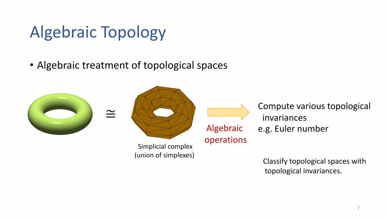
Algebraic Topology

• Algebraic treatment of topological spaces

7

≅Algebraic operations

Compute various topological invariances

e.g. Euler number

Simplicial complex(union of simplexes)

Classify topological spaces with topological invariances.

• Homology group: independent “holes”

8

𝐻𝑘(𝑋): 𝑘-th homology group of topological space 𝑋 (𝑘 = 0,1,2,…)

𝐻0(𝑋): connected components𝐻1(𝑋): rings𝐻2(𝑋): cavities

…

≅

≅

≅

𝐻0(𝑋)

ℤ⊕ ℤ

0

0

0 ℤ

0

0

0ℤ

ℤ

ℤ

𝐻1(𝑋) 𝐻2(𝑋)

ℤ≅

ℤ ℤ⊕ ℤThe generators of 1st homology group

𝑘-dimensional holes

ℤ

Topology of statistical data?

9

Noisy finitesample

True structure

휀 −balls(e.g. manifold learning)

Small 휀 disconnected object

Large 휀 small ring is not visible

Stable extraction of topology is NOT easy!

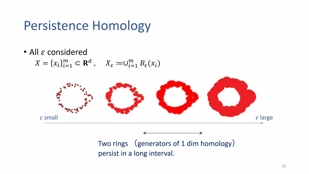
Persistence Homology

• All 휀 considered𝑋 = 𝑥𝑖 𝑖=1

𝑚 ⊂ 𝐑𝑑 , 𝑋𝜀 ≔∪𝑖=1𝑚 𝐵𝜀(𝑥𝑖)

10

휀 small 휀 large

Two rings （generators of 1 dim homology）

persist in a long interval.

• Persistence homology (formal definition)Filtration of topological spaces X ∶ 𝑋1 ⊂ 𝑋2 ⊂ ⋯ ⊂ 𝑋𝐿

𝑃𝐻𝑘(X): 𝐻𝑘 𝑋1 → 𝐻𝑘 𝑋2 → ⋯ → 𝐻𝑘(𝑋𝐿) ≅⊕𝑖=1𝑚𝑘 𝐼[𝑏𝑖 , 𝑑𝑖]

𝐼 𝑏, 𝑑 ≅ 0 → ⋯ → 0 → 𝐾 → ⋯ → 𝐾 → 0 → ⋯ → 0

11

at 𝑋𝑏 at 𝑋𝑑𝐾: field

Irreducible decomposition

The lifetime (birth, death) of each generator is rigorously defined,and can be computed numerically.

Birth and death of a generator of 𝑃𝐻1(𝑋)

• Two popular (equivalent) expressions of PH

12

𝛼

휀

Barcodes and PD are considered for each dimension.

Bar from the birth to death of each generator

Barcode Persistence diagram (PD)

Plots of the birth (b) and death (d)of each generator of PH in a 2D graph (𝑑 ≥ 𝑏).

Handy descriptors or features of complex geometric objects

Beyond topology

• PH contains geometrical information more than topology

13

Barcodes of 1-dim PH

휀

Statistical approach with kernels to topological data analysis

14

Statistical approach to TDA

• Conventional TDA

15

Data Computation of PH Visualization（PD） Analysis by experts

SoftwareCGAL / PHAT

CGAL: The Computational Geometry Algorithms Library http://www.cgal.org/PHAT: Persistent Homology Algorithm Toolbox https://bitbucket.org/phat-code/phat

e.g. Molecular dynamics simulation

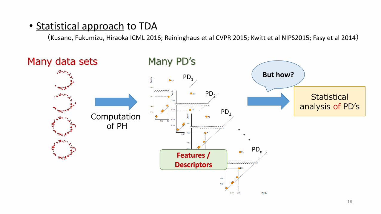
• Statistical approach to TDA（Kusano, Fukumizu, Hiraoka ICML 2016; Reininghaus et al CVPR 2015; Kwitt et al NIPS2015; Fasy et al 2014）

16

Many data sets

Computation of PH

PD1

PD2

PD3

PDn

Many PD’s

Statistical analysis of PD’s

Features / Descriptors

But how?

Kernel representation of PD

• Vectorization of PD by positive definite kernel

• PD = Discrete measure 𝜇𝐷 ≔ σ𝑧∈𝑃𝐷 𝛿𝑧

• Kernel embedding of PD’s into RKHS

ℇ𝑘: 𝜇𝐷 ↦ ∫ 𝑘 ⋅, 𝑥 𝑑𝜇𝐷 𝑥 = σ𝑖 𝑘(⋅, 𝑥𝑖) ∈ 𝐻𝑘, Vectorization

• For some kernels (e.g., Gaussian, Laplace), ℇ𝑘 is injective.

• By vectorization,

• a number of methods for data analysis can be applied,SVM, regression, PCA, CCA, etc.

• tractable computation is possible with kernel trick. 17

𝑘: positive definite kernel𝐻𝑘: corresponding RKHS

Persistence Weighted Gaussian (PWG) Kernel

Generators close to the diagonal may be noise, and should be discounted.

𝑘𝑃𝑊𝐺 𝑥, 𝑦 = 𝑤 𝑥 𝑤 𝑦 exp −𝑦−𝑥 2

2𝜎2

𝑤 𝑥 = 𝑤𝐶,𝑝 𝑥 ≔ arctan 𝐶Pers 𝑥 𝑝 (𝐶, 𝑝 > 0)

Pers 𝑥 ≔ 𝑑 − 𝑏 for 𝑥 ∈ { 𝑏, 𝑑 ∈ 𝐑2|𝑑 ≥ 𝑏}

18

Pers(x1)

• Stability with PWG kernel embedding• PWGK defines a distance on the persistence diagrams,

𝑑𝑘 𝐷1, 𝐷2 ≔ ℇ𝑘 𝐷1 − ℇ𝑘 𝐷2 𝐻𝑘, 𝐷1, 𝐷2: persistence diagrams

Stability Theorem (Kusano, Hiraoka, Fukumizu 2015)

𝑀: compact subset in 𝐑𝑑. 𝑆 ⊂ 𝑀, 𝑇 ⊂ 𝐑𝑑: finite sets.

If 𝑝 > 𝑑 + 1, then with PWG kernel (𝑝, 𝐶, 𝜎),

𝑑𝑘 𝐷𝑞(𝑆), 𝐷𝑞(𝑇) ≤ 𝐿 𝑑𝐻 𝑆, 𝑇 .

𝐿: constant depending only on 𝑀, 𝑝, 𝑑, 𝐶, 𝜎

𝐷𝑞(𝑆): 𝑞 th persistence diagram of 𝑆

𝑑𝐻: Haussdorff distance

This stability is NOT known for Gaussian kernel.

19

A small change of a setcauses only a smallchange in PD

Lipschitz continuity

2nd-level kernel

2nd-level kernel (SVM for measures, Muandet, Fukumizu, Dinuzzo, Schölkopf 2012)

• RKHS-Gaussian kernel 𝐾 𝜑1, 𝜑2 = exp −𝜑1−𝜑2 𝐻𝑘

2

2𝜏2

derives

𝐾 𝐷𝑖 , 𝐷𝑗 = exp −ℇ𝑘(𝐷𝑖)−ℇ𝑘(𝐷𝑗) 𝐻𝑘

2

2𝜏2

20

PD1

PD2

PD3

PDm

ℇ𝑘 𝑃𝐷1ℇ𝑘 𝑃𝐷2

…ℇ𝑘 𝑃𝐷𝑚

Vectors in RKHSPD’sData sets

Application of pos. def. Kernel on RKHS

𝐷𝑖 , 𝐷𝑗: Persistence diagrams

Data analysis method

Embedding

Computational issue

The number of generators in a PD may be large (≥ 103, 104 )

For 𝑃𝐷𝑖 = σ𝑎=1𝑁𝑖 𝛿

𝑥𝑎(𝑖) ∪ Δ， 𝐾 𝑃𝐷𝑖 , 𝑃𝐷𝑗 = exp −

ℇ𝑘(𝑃𝐷𝑖)−ℇ𝑘(𝑃𝐷𝑗) 𝐻𝑘

2

2𝜏2requires

computation

ℇ𝑘(𝑃𝐷𝑖) − ℇ𝑘(𝑃𝐷𝑗) 𝐻𝑘

2

= σ𝑎 =1𝑁𝑖 σ𝑏 =1

𝑁𝑖 𝑘 𝑥𝑎𝑖, 𝑥𝑏

𝑖+ σ

𝑎 =1

𝑁𝑗 σ𝑏 =1

𝑁𝑗 𝑘 𝑥𝑎𝑗, 𝑥𝑏

𝑗− 2σ𝑎 =1

𝑁𝑖 σ𝑏 =1

𝑁𝑗 𝑘 𝑥𝑎𝑖, 𝑥𝑏

𝑗.

The number of exp −𝑥𝑎−𝑥𝑏

2

2𝜎2＝ 𝑂(𝑚2𝑁2) computationally expensive for

𝑁 ≈ 104

21

𝑁 = max{𝑁𝑖|𝑖 = 1,… , 𝑛}

• Approximation by random features (Rahimi & Recht 2008)

By Bochner’s theorem

exp −𝑥𝑎−𝑥𝑏

2

2𝜎2= 𝐶 ∫ 𝑒 −1𝜔𝑇 𝑥𝑎−𝑥𝑏

𝜎2

2𝜋𝑒−

𝜎2 𝜔 2

2 𝑑𝜔

Approximation by sampling: 𝜔1, … , 𝜔𝐿: 𝑖. 𝑖. 𝑑. ~ 𝑄𝜎

exp −𝑥𝑎−𝑥𝑏

2

2𝜎2≈ 𝐶

1

𝐿σℓ=1𝐿 𝑒 −1𝜔ℓ

𝑇𝑥𝑎 𝑒 −1𝜔ℓ𝑇𝑥𝑏

σ𝑎 =1𝑁𝑖 σ

𝑏 =1

𝑁𝑗 𝑘 𝑥𝑎𝑖, 𝑥𝑏

𝑗≈

𝐶

𝐿σ𝑎 =1𝑁𝑖 σ

𝑏 =1

𝑁𝑗 σℓ=1𝐿 𝑤 𝑥𝑎

𝑖𝑤 𝑥𝑏

𝑗𝑒 −1𝜔ℓ

𝑇𝑥𝑎(𝑖)

𝑒 −1𝜔ℓ𝑇𝑥𝑏

(𝑗)

=𝐶

𝐿σℓ =1𝐿 σ𝑎 =1

𝑁𝑖 𝑤 𝑥𝑎𝑖

𝑒 −1𝜔ℓ𝑇𝑥𝑎

(𝑖)σ𝑏=1

𝑁𝑗 𝑤 𝑥𝑏𝑗

𝑒 −1𝜔ℓ𝑇𝑥𝑏

(𝑗)

Computational cost 𝑂(𝐿𝑁) 2nd level Gram matrix 𝑂(𝑚𝐿𝑁 +𝑚2𝐿). c.f. 𝑂(𝑚2𝑁2)

Big reduction if 𝐿, 𝑛 ≪ 𝑁

22

Gaussian distribution =:𝑄𝜎

𝐿 dim.

（Fourier transform）

Comparison: Persistence Scale Space Kernel(Reininghaus et al 2015)

• PSS Kernel

𝑘𝑅 𝑥, 𝑦 =1

8𝜋𝑡exp

𝑥 − 𝑦 2

8𝑡− exp

𝑥 − ത𝑦 2

8𝑡

ത𝑦 = (𝑑, 𝑏) for 𝑦 = (𝑏, 𝑑).

ℇ𝑘(𝐷) is considered.

• Comparison between PWGK and PSSK • PWGK can control the discount around the diagonal independently of the

bandwidth parameter.

• PSSK is not shift-invariant Random feature approximation is not applicable.

• In Reininghaus et al 2015, 2nd level kernel is not considered.

23

Pos. def. on 𝑏, 𝑑 𝑑 ≥ 𝑏0 on Δ.

S0

S1

S1

noise

Data points 1

Data points 2

No S0

Synthetic example: SVM classification

• Classification of PD’s by SVM• One big circle (random location and sample size) 𝑆1

with or without small circle 𝑆0.

• 𝑌 = XOR(𝑍1, 𝑍2)

• 𝑍1: Does S0 exists? Yes/No

• 𝑍2: Is the generator of S1 within ((b(𝑆1)<1 && d(𝑆1))? Yes/No

• Noise is added, in fact.

• 100 for training and 100 for testing

• Result (correct classification)

• PWGK (proposed): 83.8%

• PSSK (comparison): 46.5%

24

S1

S0

PD1𝑌 = 1

Applications

25

Application 1: Transition of Silica (SiO2 )

If cooled down rapidly from the liquid state, SiO2 changes into the glass state (not to crystal).

Goal: identify the temperature of phase transition.

Data: Molecular Dynamics simulation for SiO2. 3D arrangements of the atoms are used for computing PD at 80 temperatures. (Nakamura et al 2015; Hiraoka et al 2015)

26

Examples of PD’s

Liquid Glass (Amorphous)

Amorphous: “soft” structure

27

Change point detection

• Data along a parameter 𝑡𝑋𝑡, 𝑡 = 1,… , 𝑇.

Kernel Change Point Analysis with Fisher Discriminant score (Harchoui et al 2009):

For each 𝑡, two classes are defined by the data before and after 𝑡. Fisher score on RKHS is used.

• For each 𝑡, compute ෝ𝑚1:𝑡 =1

𝑡σ𝑖=1𝑡 Φ(𝑋𝑖) and ෝ𝑚𝑡+1:𝑇 =

1

𝑇−𝑡σ𝑖=𝑡+1𝑇 Φ(𝑋𝑖).

• Compute Δ𝑡 ≔ 𝑉1:𝑡 + 𝑉𝑡+1:𝑇 + 𝛾𝐼 −1

2( ෝ𝑚1:𝑡 − ෝ𝑚𝑡+1:𝑇) 𝐻𝑘

2

.

• Find max𝑡

Δ𝑡.

• For the packing problem, 𝑋𝑡 = ℇ𝑘 𝐷𝜙𝑡 (𝑡 = 1,… , 80).28

Change point𝑡

• Detection of liquid-glass state transition• Approach in physics:

Estimation using derivatives of enthalpy curve, but not so accurate.

• Our approach: purely data-driven

Persistence diagrams, and then change point detection by Kernel FDR.

• Number of generators in a PD is 30000 at most difficult to use PSSK directly

• PWGK (proposed) is applied with random features.

29

30

Detected change point = 3100K

Enthalpy by physicist: [2000K, 3500K]Δ𝑡

• 2-dim plot by Kernel PCA

31

Sharp change between the two phases.

(Colored by the result of change point detection. Colors are not used for KPCA).

The result indicates that the phase can be identified by the snap-shot, while this is still controversial among physicists.

Liquid state

glass state

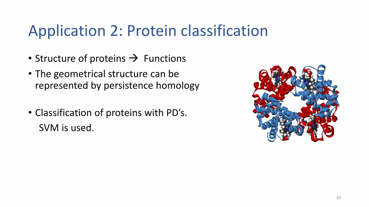
Application 2: Protein classification

• Structure of proteins Functions

• The geometrical structure can be represented by persistence homology

• Classification of proteins with PD’s.

SVM is used.

32

• Data A: Protein-drug binding

• M2 channel in the influenza A virus:a target of medicine.Biding an inhibitor changes the structure

• Task: Determine from the structure if there is rimantadine (inhibitor) in the M2 channel.

• Data: 3D-structures from NMR• 15 data for each of binding / non-binding. • Random choice of 10 training samples for each class. The rest is used for testing.

100 random choices for CV.

33

Cang, Mu, Wu, Opron, Xia, Wei, Molecular Based Mathematical Biology (2015) Fig. 3

• Data B: 2 states of hemoglobin

• Task: classify of the 2 states Relaxed (R) / Taut (T)

• Data: 3D-stturcures from X-ray diffraction

• R: 9 data, T: 10 data

• Choice of one data from each class for testing, and the rest used for training.

• All combinations are used for CV.

34

Relaxed (R) Taut (T)

Cang, Mu, Wu, Opron, Xia, Wei, Molecular Based Mathematical Biology (2015) Fig. 4

• Results• Comparison with Cang et al (2015), where PH is used with 13 dimensional hand-

made Molecular Topological Fingerprint (MTF) .

• PWGK + SVM: only 1st PH is used.

35

A. Protein-Drug B. Hemoglobin

PWGK 100 88.90

MTF* (nbd) 93.91 / (bd) 98.31 84.50

# Dim Description

1 0 2nd longest lifetime

2 0 3rd longest lifetime

3 0 Total sum of lifetme

4 0 Average lifetime

5 1 Birth point of the longest generator

6 1 Longest lifetime

7 1 Birth points of the shortest generator among lifetime ≥1.5Å

8 1 Ave. medium points of generators among lifetime ≥1.5Å

9 1 Number of generators in [4.5, 5.5]Å, divided by total #atoms.

10 1 Number of generators in [3.5, 4.5)Å and (5.5, 6.5]Å, divided by total #atoms.

11 1 Total sum of lifetmes

12 1 Average lifetime

13 2 The birth point of the first generator.

MTF

CV classification rates

* Results of MTF are taken from Cang et al. Molecular Based Mathematical Biology (2015).

Conclusion

• Topological data analysis• Key technology = persistence homology

• PH can introduce useful features / descriptors for complex geometrical structures.

• PH contains information more than topology.

• Statistical approach to topological data analysis• Statistical data analysis on many persistence diagrams.

• Kernel methods introduce systematic data analysis to TDA.

• Vectorization of persistence diagrams by kernel embedding.

• Persistence weighted Gaussian kernel flexible kernel for noise.

36

References

Kusano, G., Fukumizu, K., Hiraoka, Y. (2015) Persistence weighted Gaussian kernel for topological data analysis. Proc. Intern. Conf. Machine Learning 2016

Carlsson, G. (2009) Topology and data. Bull. Amer. Math. Soc., 46(2):255–308. http://dx.doi.org/10.1090/S0273-0979-09-01249-X .

Hiraoka, Y., Nakamura, T., Hirata, A., Escolar, E. G., Matsue, K., and Nishiura, Y. (2016) Description of medium-range order in amorphous structures by persistent homology. PNAS, 113(26), 7035–7040.

Nakamura, T., Hiraoka, Y., Hirata, A., Escolar, E. G., and Nishiura, Y. (2015) Persistent homology and many-body atomic structure for medium-range order in the glass. Nanotechnology, 26 (304001).

Reininghaus, J., Huber, S., Bauer, U., and Kwitt, R. (2015) A stable multi-scale kernel for topological machine learning. Proc. IEEE Conf. on Computer Vision and Pattern Recognition (CVPR), pp. 4741–4748.

Kwitt, R., Huber, S., Niethammer, M., Lin, W., and Bauer, U. (2015) Statistical topological data analysis - a kernel perspective. Advances in Neural Information Processing Systems 28, pp. 3052–3060.

Fasy, B. T., Lecci, F., Rinaldo, A., Wasserman, L., Balakrishnan, S., and Singh, A. (2014) Confidence sets for persistence diagrams. The Annals of Statistics, 42(6):2301–2339,

Cang, Z., Mu, L., Wu, K., Opron, K., Xia, K., and Wei, G. W. (2015) A topological approach for protein classification. Molecular Based Mathematical Biology, 3(1), 2015

37