ASYMPTOTIC NEAR-MINIMAXITY OFTHE RANDOMIZED SHIRYAEV–ROBERTS–POLLAK

CHANGE-POINT DETECTION PROCEDUREIN CONTINUOUS TIME∗

ALEKSEY S. POLUNCHENKO†

Abstract. For the classical continuous-time quickest change-point detection problem it is shownthat the randomized Shiryaev–Roberts–Pollak procedure is asymptotically nearly minimax-optimal(in the sense of Pollak [14]) in the class of randomized procedures with vanishingly small false alarmrisk. The proof is explicit in that all of the relevant performance characteristics are found analyticallyand in a closed form. The rate of convergence to the (unknown) optimum is elucidated as well. Theobtained optimality result is a one-order improvement of that previously obtained by Burnaev etal. [4] for the very same problem.

Key words. Minimax optimality, Optimal stopping, Quasi-stationary distribution, Sequentialchange-point detection, Shiryaev–Roberts procedure

AMS subject classifications. 60G35, 60G40, 93E10, 62L10, 62L15

1. Introduction, problem formulation and significance. This work’s focusis on the classical minimax change-point detection problem where the aim is to detect(in an optimal manner) a possible onset of a drift in “live”-observed standard Brow-nian motion. More formally, suppose one is able to observe a “live” process, (Xt)t>0,that is governed by the stochastic differential equation (SDE):

(1) dXt = µ1lt>θdt+ dBt, t > 0, with X0 = 0,

where (Bt)t>0 is standard Brownian motion (i.e., E[dBt] = 0, E[(dBt)2] = dt, and

B0 = 0), µ 6= 0 is the known post-change drift magnitude, and θ ∈ [0,∞] is theunknown (nonrandom) change-point; the notation θ = 0 (θ =∞) is to be understoodas the case when E[Xt] = 0 (E[Xt] = µt) for all t > 0. One’s objective is to establishonline that the process’ drift is no longer zero, and do so in an optimal fashion, i.e.,as quickly as is possible within an a priori set level of the false alarm risk.

Let Ω , C[0,+∞) be the space of continuous functions on R+ , [0,+∞). Let(Ft)t>0, Fs ⊆ Ft for 0 6 s < t, denote the filtration generated by (Xt)t>0, i.e.,Ft , σ(Xs, 0 6 s 6 t) for t > 0 and F0 is the trivial σ-algebra; note that (Ft)t>0

can be seen from (1) to coincide with the filtration generated by the Brownian motion(Bt)t>0 for any θ ∈ [0,∞]. Let F , F∞ , ∨t>0 Ft. With model (1) placed onthe filtered probability space (Ω,F , (Ft)t>0,P) any change-point detection procedureis a (Ft)t>0-measurable stopping time, τ , τ(ω), ω ∈ Ω, i.e., ω : τ(ω) 6 t ∈ Ftfor all t > 0. The interpretation of τ is that it is a rule to stop and declare that(Xt)t>0 has (apparently) gained a drift of magnitude µ 6= 0. The decision made atstopping need not be correct. A “good” (i.e., optimal or nearly optimal) detectionprocedure τopt is one that minimizes (or nearly minimizes) the desired detection delaypenalty, subject to a constraint on the false alarm risk. See, e.g., [29, 17], [24], [25,Chapter VI], or [28, Part II] for a survey of the major existing optimality criteria.

∗Submitted to the editors DATE.Funding: This work was partially supported by the Simons Foundation via a Collaboration

Grant in Mathematics under Award # 304574.†Department of Mathematical Sciences, State University of New York at Binghamton, Bingham-

ton, NY 13902–6000, USA (aleksey@binghamton.edu, http://people.math.binghamton.edu/aleksey).

1

arX

iv:1

607.

0329

4v4

[m

ath.

ST]

10

Apr

201

7

2 A. S. POLUNCHENKO

The specific one considered in this work is the minimax criterion of Pollak [14]. Seealso [4, 7] where Pollak’s [14] criterion is referred to as “Variant (C)” of the quickestchange-point detection problem. We now introduce it formally, following the originalnotation of [4, 7].

Let Pθ , Law(X|P, θ) denote the probability measure (distribution law) in-duced by the observed process, (Xt)t>0, under the assumption that the change-point,θ ∈ [0,+∞], is fixed; note that P∞ is the Wiener measure. Let Eθ represent the re-spective Pθ-expectation operator. Pollak’s [14] minimax version (or “Variant (C)” inthe terminology used in [4, 7]) of the quickest change-point detection problem assumesthat the false alarm risk is measured in terms of the classical Average Run Length(ARL) to false alarm metric defined as E∞(τ), and the cost of a delay to (correct)detection is quantified via the largest (conditional) Average Detection Delay definedas

(2) C(τ) , supθ>0

C(τ, θ) where C(τ, θ) , Eθ(τ − θ|τ > θ) for θ > 0,

and the idea is to consider

(3) MT ,τ : E∞(τ) = T

where T > 0 is given,

i.e., the class of detection procedures (stopping times) τ with the ARL to false alarmset at a given level T > 0, and

(4) seek τopt ∈MT such that C(τopt) = C(T ) where C(T ) , infτ∈MT

C(τ),

for any T > 0.Problem (4) is a major open problem in all of quickest change-point detection:

although it has been attacked repeatedly (see, e.g., [34, 12, 31, 16]), its general solutionis yet to be found, not only in the discrete-time setting, but in the continuous-timesetting as well. The current “favorite” in the search for the solution seems to be theGeneralized Shiryaev–Roberts (GSR) procedure of Moustakides et al. [13]. The GSRprocedure is a headstarted version of the classical quasi-Bayesian Shiryaev–Roberts(SR) procedure of Shiryaev [19, 20] and Roberts [18]. Specifically, tailored to theBrownian motion scenario (1), the GSR procedure calls for stopping at:

(5) τ(x)A , inf

t > 0: ψ

(x)t > A

such that inf

∅

=∞,

where A > 0 is a detection threshold (set in advance so as to keep the “false positive”

risk tolerably low, i.e., to guarantee E∞(τ(x)A ) = T for a given T > 0), and the GSR

statistic (ψ(x)t )t>0 is the diffusion process that solves the SDE:

(6) dψ(x)t = dt+ µψ

(x)t dXt with ψ

(x)0 , x > 0,

where dXt is as in (1) above. The initial value ψ(x)0 , x is sometimes referred to as the

headstart. The term “Generalized Shiryaev–Roberts procedure” appears to have beencoined in [30], and was motivated by the fact that, in the no-headstart case, i.e., whenx = 0, the GSR procedure (5)-(6) reduces to the classical SR procedure [19, 20, 18].Continuing to adhere to the notation used in [4, 7], we, too, shall denote the classicalSR procedure’s stopping time as τA and its underlying statistic as ψt, i.e., define

τA , τ(0)A and ψt , ψ

(0)t .

ON OPTIMALITY OF THE SHIRYAEV–ROBERTS–POLLAK PROCEDURE 3

The reasons to suspect that the GSR procedure might actually solve problem (4)are three. The first reason is the result obtained (for the discrete-time analogue ofthe problem) in [31, 16] where the GSR procedure with a “finetuned” headstart wasexplicitly demonstrated to be exactly Pollak-minimax in two specific (discrete-time)scenarios. The second reason is the general so-called almost Pollak-minimaxity ofthe GSR procedure (again, with a carefully designed headstart) established (in thediscrete-time setting) in [30]. More specifically, it was shown in [30] that, if, for a givenT > 0, the GSR procedure’s detection threshold A = AT > 0 and headstart x = xT >0 are set so that τ

(xT )AT

∈MT , but xT = o(AT ) in the sense that limT→+∞(xT /AT ) = 0,then

C(τ(xT )AT

)− C(T ) = oT (1) as T → +∞,

where C(τ) and C(T ) are as in (2) and (4), respectively, and oT (1)→ 0 as T → +∞;see [3] for an attempt to generalize this result to the continuous-time model (1). Since

obviously C(τ(xT )AT

) → +∞ and C(T ) → +∞ as T → +∞, the above is effectivelysaying that the GSR procedure is nearly Pollak-minimax-optimal, whenever the ARLto false alarm level T > 0 is large. This is a strong optimality property known in theliterature (see [30]) as order-three asymptotic (as T → +∞) Pollak-minimaxity (ornear Pollak-minimaxity).

However, the most important reason to study the GSR procedure deeper is thefollowing: while the general solution τopt to Pollak’s [14] problem (4) is still un-known, there is a universal “recipe” (also proposed by Pollak [14]) to achieve nearPollak-minimaxity, and the GSR procedure is the main ingredient of the “recipe”.

Specifically, Pollak’s [14] ingenious idea was to start the GSR statistic (ψ(x)t )t>0 off

a random number sampled from the statistic’s so-called quasi-stationary distribution(formally defined below). For the discrete-time version of the problem, Pollak [14]was able to prove that such a randomized “tweak” of the GSR procedure is nearlyPollak-minimax; see also [30, Theorem 3.4]. It is to extend this result to the Brownianmotion scenario (1) that is the objective of this work.

The randomization of the GSR procedure’s headstart necessitates the introductionof a probability space larger than the original (Ω,F , (Ft)t>0,P) constructed above.To that end, a suitable extension, which we shall denote (Ω,F , (F t)t>0,P), has al-ready been offered in [4] and in [20, Chapter II, Section 7], and the ingredients are:1. Ω , Ω× Ω, where Ω , [0, 1]; 2. F , F ⊗ F and F t , Ft ⊗ F for all t > 0, whereF , B(Ω) is a Borel system of subsets on Ω; and 3. P , P⊗ P, where P is a Lebesguemeasure on (Ω, F). See also [25].

To place Pollak’s [14] problem (4) on the new probabilistic basis (Ω,F , (F t)t>0,P),

define Pθ , Pθ⊗P for θ ∈ [0,+∞], and let Eθ denote the corresponding Pθ-expectationoperator. It is natural to measure the ARL to false alarm of a randomized procedureτ , τ(ω), ω , (ω, ω) ∈ Ω, in terms of E∞(τ), and the worst Average Detection Delayvia

(7) C(τ) , supθ>0

C(τ , θ) where C(τ , θ) , Eθ(τ − θ|τ > θ) for θ > 0.

Problem (4) can now be extended as follows. Consider

(8) MT ,τ : E∞(τ) = T

where T > 0 is given,

i.e., the class of randomized detection procedures (randomized stopping times) τ with

4 A. S. POLUNCHENKO

the ARL to false alarm set at a given level T > 0, and

(9) seek τopt ∈MT such that C(τopt) = C(T ) where C(T ) , infτ∈MT

C(τ),

for any T > 0.Problem (9), just as problem (4), is also still open, whether in discrete- or in

continuous-time settings. It is referred to as “Variant (C)” of the quickest change-point detection problem in [4]. While “Variant (C)” and “Variant (C)” are similar,they are not the same, because MT ⊂ MT for any fixed T > 0, as can be seen fromdefinitions (3) and (8). Put another way, randomized detection procedures with theARL to false alarm set at a prescribed level T > 0 form a larger family than dotheir nonranomized counterparts with the same ARL to false alarm level T > 0. As aresult, even though neither C(T ) nor C(T ) is known, it is apparent that C(T ) 6 C(T )for any fixed T > 0. This work’s specific focus is on problem (9), and our “courseof attack” is exactly the same as that of Pollak [14] who considered the problem’sdiscrete-time analogue and nearly solved it.

The main ingredient of Pollak’s [14] solution strategy is the quasi-stationary dis-tribution of the SR statistic (ψt)t>0. Formally, this distribution is defined as

(10) QA(x) , limt→+∞

P∞(ψt 6 x|τA > t) with qA(x) ,d

dxQA(x) where x ∈ [0, A],

and its existence follows, e.g., from the fundamental work of Mandl [11]; see also,e.g., [5] and [6, Section 7.8.2]. The density qA(x) was studied in [4] where the authorsobtained a large-A order-one expansion of qA(x). However, a more detailed investi-gation of the distribution and its properties was recently carried out in [15] wherenot only QA(x) and qA(x) were both expressed analytically and in a closed form,but also the density qA(x) was shown to be unimodal, its entire moment series wascomputed, and more accurate (up to the third order) large-A approximations of qA(x)were obtained as well. These results will play a critical role in the sequel.

The decision statistic behind Pollak’s [14] randomized version of the GSR proce-dure is the solution (ψ∗t )t>0 , (ψ∗t (ω))t>0 of the SDE:

(11) dψ∗t = dt+ µψ∗t dXt with ψ∗0 ∝ QA(x),

where dXt is as in (1) and QA(x) is defined in (10). The corresponding stopping timeis as follows:

(12) τ∗A , inft > 0: ψ∗t > A

such that inf

∅

=∞,

and we shall follow [30] and refer to it as the (randomized) Shiryaev–Roberts–Pollak(SRP) procedure.

Pollak’s [14] motivation to introduce and study the SRP procedure (12)-(11) wasto get the detection delay penalty C(τ , θ) given by (7) independent of the change-pointθ, i.e., to achieve

Eθ(τ∗A) , C(τ∗A, 0) ≡ C(τ∗A, θ) , Eθ(τ∗A − θ|τ∗A > θ) for any θ > 0 and A > 0,

so that

(13) supθ>0

Eθ(τ∗A − θ|τ∗A > θ) , C(τ∗A) ≡ C(τ∗A, 0) , Eθ(τ∗A) for any A > 0.

ON OPTIMALITY OF THE SHIRYAEV–ROBERTS–POLLAK PROCEDURE 5

The foregoing delay-risk-equalization is a direct consequence of the fact that, bydesign, the process (ψ∗t )t>0 has a time-invariant probabilistic structure, i.e., P∞(ψ∗t 6x|τ∗A > t) = P∞(ψ∗t 6 x|ψ∗s < A, s 6 t) = QA(x) for all t > 0. A risk-equalizing prop-erty akin to (13) is known in the general decision theory (see, e.g., [8, Theorem 2.11.3])to be a necessary condition for strict minimaxity. Hence the introduction of the SRPprocedure by Pollak in [14] was, in a way, Pollak’s attempt to solve his very ownminimax version of the quickest change-point detection problem, although consideredonly in the discrete-time setting. As was mentioned earlier, Pollak [14] succeeded inproving only that the SRP procedure is asymptotically order-three Pollak-minimax;the result was recently reobtained in [30] through a different approach. It is reasonableto expect the same result to hold for the continuous-time model (1) as well. To thatend, in [4], the SRP procedure τ∗A given by (12)-(11) was shown to be asymptoticallyPollak-minimax in the class of randomized procedures MT , but only up to the secondorder, i.e., the delay risk C(τ) is minimized up to an additive term that goes to apositive constant as the false alarm risk vanishes. That is, if, for a given T > 0, theSRP procedure’s threshold A = AT > 0 is set so that τ∗A ∈MT , then

(14) C(τ∗AT)− C(T ) = OT (1) as T → +∞,

where OT (1)→ const > 0 as T → +∞.We are now in a position to formally state the specific contribution of this work:

it is shown in the sequel that the SRP procedure τ∗A is almost Pollak-minimax amongall reasonable randomized detection procedures. That is, if, for a given T > 0, theSRP procedure’s threshold A = AT > 0 is set so that τ∗A ∈MT , then

(15) C(τ∗AT)− C(T ) = oT (1) as T → +∞,

where we reiterate that oT (1) → 0 as T → +∞. This is a one-order improvementof (14) previously proved in [4]. Moreover, it is also shown in the sequel that the

“oT (1)” sitting in the right-hand side of (15) vanishes no slower than 1/√µ2T as

T → +∞.

2. Summary of relevant prior results. Our proof of (15) utilizes certainresults established in the literature earlier. Hence, to streamline the proof, this sectionsummarizes the relevant prior results. To that end, the latter can be divided upinto two categories. Category 1 includes results that concern properties of the GSRprocedure (5)-(6), including the classical SR procedure [19, 20, 18] as its particularcase. These results are all due to A.N. Shiryaev and his co-authors. By contrast,Category 2 is comprised of results on properties of the randomized SRP procedure (12)-(11). These results all come from [15] and concern the SR statistic’s quasi-stationarydistribution defined in (10).

We start by going over the first group of results. The first result is the fact that,for any given T > 0, the unknown optimal delay risks C(T ) and C(T ) defined in (4)and in (9), respectively, both permit an explicitly computable lowerbound. Specifically,the following inequalities hold true

(16) B(T ) 6 C(T ) and B(T ) 6 C(T ) for any T > 0,

where

B(T ) , infτ∈MT

1

T

∫ ∞0

Eθ(τ − θ)+dθ and B(T ) , infτ∈MT

1

T

∫ ∞0

Eθ(τ − θ)+dθ,

6 A. S. POLUNCHENKO

where x+ , max0, x; cf. [7, 4]. The quantities B(T ) and B(T ) are the optimalgeneralized Bayesian risks: they quantify the delay cost when θ is random and sampledfrom an improper uniform distribution on [0,+∞). See [22, 23, 26].

A remarkable fact about B(T ) and B(T ) is that B(T ) = B(T ) for any T > 0.See [21, Chapter II, Section 7] and [25, Chapter VI]. Moreover, both B(T ) and B(T )permit the following explicit (and amenable to numerical evaluation) representation:

(17) B(T ) = B(T ) =2

µ2

F(

2

µ2T

)− 1 +

2

µ2T

∫T

0

F

(2

µ2x

)dx

x

,

where

(18) F (x) , ex E1(x)

with

(19) E1(x) ,∫ +∞

x

e−tdt

t, x > 0,

being the so-called exponential integral, a special function often also denoted as−Ei(−x); see, e.g., [9] and [1, Chapter 5]. Formula (17) is a straightforward gen-eralization of [7, Theorem 2.3] which gives the formula only in the special case ofµ =√

2. It is now apparent (cf. [7, Theorem 4.4]) that B(T ) = B(T ) 6 C(T ) 6 C(T )for any T > 0.

The third result is a classical property of the GSR procedure τ(x)A defined in (5),

namely that

(20) E∞(τ(x)A ) = A− x, for any x ∈ [0, A], with A > 0;

cf., e.g., [4, p. 530], although the result is likely to have been first discovered by A.N.Shiryaev in the early 1960’s. In the special case of no headstart, formula (20) reduces

to the equally well-known fact that E∞(τ(x)A ) = A for any A > 0; incidentally, the

formula E∞(τ(x)A ) = A is involved in the derivation of (17). It will also prove useful to

point out that one way to arrive at (20) is to notice that the process (ψ(x)t − t−x)t>0

is a zero-mean P∞-martingale, i.e., E∞(ψ(x)t − t − x) = 0 for any t > 0 and x ∈

[0, A], and then invoke Doob’s optional stopping theorem to deduce that E∞(τ(x)A ) =

E∞(ψ(x)

τ(x)A

)− x, and then finally make the transition to (20) by arguing that the GSR

statistic (ψ(x)t )t>0 reaches any level A > 0 almost surely, so that ψ

(x)

τ(x)A

= A with

probability 1, under any measure Pθ.The forth result is yet another classical property of the GSR procedure, namely

that

(21) E0(τ(x)A ) , C(τ

(x)A , 0) =

2

µ2

F

(2

µ2A

)− F

(2

µ2x

), x ∈ [0, A],

where F (x) is the function introduced in (18). This formula is a trivial generalizationof [7, Lemma 3.3] where it was established in the special case of µ =

√2. It is worth

mentioning that formula (21), just as formula (20), is also involved in the proof of (17).

ON OPTIMALITY OF THE SHIRYAEV–ROBERTS–POLLAK PROCEDURE 7

The fifth and final result to go into the first category is the assertion that

(22)2

µ2T

∫T

0

F

(2

µ2x

)dx

x= O

(log2(µ2T )

µ2T

)as T → +∞,

which follows from [7, Formulae (2.33) and (2.34), p. 456]. It is also noteworthy thatthe quantity sitting in the left-hand side of (22) is nonnegative for any T > 0.

We now switch attention to the second group of results, which all revolve aroundthe formula

(23) C(τ∗A) =

∫A

0

C(τ(x)A , 0) qA(x) dx,

where C(τ(x)A , 0) , E0(τ

(x)A ) is given explicitly by (21) above, and qA(x) is the pdf of

the GSR statistic’s quasi-stationary distribution formally defined in (10). It is evidentfrom formula (23) getting C(τ∗A) expressed explicitly is impossible without a closed-form expression for qA(x). Such an expression was recently obtained in [15], and it ispresented next.

Specifically, in [15], it was shown that, for any fixed detection threshold A > 0,the density qA(x) is given by

(24) qA(x) =

1

xe− 1µ2x W

1,ξ2

(2

µ2x

)e− 1µ2A W

0,ξ2

(2

µ2A

) 1lx∈[0,A],

while the respective cdf QA(x) is given by

(25) QA(x) =

1, for x > A;

e− 1µ2x W

0,ξ2

(2

µ2x

)e− 1µ2A W

0,ξ2

(2

µ2A

) , for x ∈ [0, A);

0, otherwise,

where

(26) ξ ≡ ξ(λ) ,

√1− 8

µ2λ,

with λ ≡ λA being the smallest nonnegative solution of the (always consistent) equa-tion

(27) W1,ξ(λ)

2

(2

µ2A

)= 0,

and Wa,b(z) is the standard notation for the special function known the WhittakerW function. The latter is defined as one of the two fundamental solutions w(z) of theso-called Whittaker [32] equation

(28)∂2

∂z2w(z) +

(−1

4+a

z+

1/4− b2

z2

)w(z) = 0, z ∈ C,

8 A. S. POLUNCHENKO

where a, b ∈ C are parameters. The second fundamental solution of the Whittakerequation (28) is known as the Whittaker M function, and it is conventionally denotedas Ma,b(z). A distinguishing feature of Ma,b(z) is that, unlike Wa,b(z), it does notexist when 2b = −1,−2,−3, . . ., and has to be regularized. See [27] and [2] for anextensive study of the Whittaker W and M functions.

Formulae (24) and (25), including condition (27), all put together make up thefirst result to go into the second group of results. In a nutshell, the formulae are thesolution of a certain Sturm–Liouville problem, and λ is the smallest eigenvalue of thecorresponding Sturm–Liouville operator. See [15, Section 2] and [4, Section 3]. Wealso remark parenthetically that the original notation used in [15] is −λ (6 0) ratherthan λ (> 0). We made this flip in the sign here entirely for convenience. We also notethat λ, as a solution of equation (28), is dependent on A > 0, and throughout what isto follow, where necessary, we shall emphasize this dependence via the notation λA.

The next result to go into Category 2 is a result also obtained in [15], and itconcerns the quasi-stationary distribution’s moments. Specifically, as shown explicitlyin [15], if Z is a random variable sampled from a population with the pdf qA(x) givenby (24), then E[Z] = A− 1/λ, and

(29) Var[Z] =λ− µ2(Aλ− 1)2

λ2(µ2 + λ),

where we reiterate that λ > 0 is the largest (nonnegative) solution of equation (27).The foregoing formulae for the first moment and variance of the quasi-stationarydistribution were obtained directly from (24) using properties of the Whittaker Wfunction.

The formula E[Z] = A − 1/λ can also be derived from (20). To that end, thekey is to recall that the P∞-distribution of the SRP procedure’s stopping time τ∗Ais exactly exponential with parameter λ, so that E∞(τ∗A) = 1/λ. Consequently, ifone now averages (20) through with respect to x assuming that x ∝ qA(x), thenE[Z] = A − 1/λ will follow easily. Since Z is a nonnegative random variable (takingvalues in the interval [0, A]), it further follows that

(30) (0 <)1

A6 λ, A > 0,

which can be interpreted thus: to achieve the same ARL to false alarm level, the SRPprocedure requires a higher detection threshold than does the classical SR procedure.This is an anticipated consequence of the randomization used to initialize the SRPstatistic.

A more useful inequality can be gleaned from the formula (29) for Var[Z]. Specif-ically, by requiring the fraction in the right-hand side of (29) to be no less than zero,after some elementary algebra, one obtains

(0 <)1

A+

1−√

4µ2A+ 1

2µ2A26 λA 6

1

A+

1 +√

4µ2A+ 1

2µ2A2,

which, in view of (30), can be “tighten up” from below to the double inequality

(31) (0 <)1

A6 λA 6

1

A+

1 +√

4µ2A+ 1

2µ2A2;

cf. [15]. Though somewhat conservative (especially when A is small), this doubleinequality will prove good enough for our purposes. An important implication of the

ON OPTIMALITY OF THE SHIRYAEV–ROBERTS–POLLAK PROCEDURE 9

inequality is that

(32) λA =1

A+O

(1

|µ|A3/2

)as A→ +∞,

which is a generalization and also a refinement of the conclusion that

(33) λA =6e

A+O

(1

A2

)as A→ +∞,

made earlier in [4, p. 528] under the assumption that µ =√

2. Recalling now thatE∞(τ∗A) = 1/λA and that E∞(τA) = A it is direct to see from (32) that

E∞(τ∗A)

E∞(τA)→ 1 as A→ +∞,

i.e., the ARL to false alarm of the SRP procedure and that of the SR procedure withthe same threshold A > 0 are approximately the same, whenever A is large. Such astrong conclusion clearly does not follow from (33).

3. Proof of asymptotic near Pollak-minimaxity of the randomized SRPprocedure. Let us now fix the SRP procedure’s ARL to false alarm level at a givenT > 0, i.e., suppose that T > 0 is given and that the SRP procedure’s thresholdA = AT > 0 is such that E∞(τ∗AT

) = T , which, by definition (8), is equivalent toτ∗AT∈MT .The gist of our strategy to prove (15), i.e., the desired near Pollak-minimaxity of

the SRP procedure, is to show that

C(τ∗AT)−B(T ) = oT (1) as T → +∞,

where oT (1) → 0 as T → +∞. The reason this is a plausible approach is because ofthe “sandwich” inequality B(T ) 6 C(T ) 6 C(τ∗AT

) implied by (16) together with the

obvious C(T ) 6 C(τ∗AT).

Since B(T ) is given explicitly by (17), the strategy could work if C(τ∗AT) were

also expressed in a closed-form. To that end, the problem is that even though all ofthe ingredients, viz. (21), (18), and (24) with (26) and (27), required to find C(τ∗AT

)in a closed-form through (23) are available, the actual evaluation of the integral inthe right-hand side of (23) is hampered by the presence of special functions in theintegrand. To boot, getting C(τ∗AT

) expressed explicitly in just any form will not do:

it needs to be in a form similar to that given by (17) for B(T ), so that the differenceC(τ∗AT

) − B(T ) (> 0) can be conveniently upperbounded. All these challenges areovercome in the following lemma.

Lemma 3.1. For any given value A > 0 of the SRP procedure’s detection thresh-old, the procedure’s delay risk C(τ∗A) permits the representation:

(34) C(τ∗A) =2

µ2

F(

2

µ2A

)− 1 +

2λ

µ2

∫A

0

F

(2

µ2x

)QA(x)

dx

x

,

where F (x) is as in (18), QA(x) is given by (25), and λ ≡ λA is determined by theequation (27). Note that formula (34) is not an inequality.

10 A. S. POLUNCHENKO

Proof. The whole problem—in view of formulae (21), (18), (23), and (24)—iseffectively to find the integral

(35) I ,

∫+∞

2µ2A

ey2 E1(y)W

1,ξ2

(y)dy

y,

where ξ ≡ ξ(λ) is given by (26) with λ > 0 determined by (27); incidentally, condi-tion (27) will prove crucial in the evaluation of I. It is worth reminding that E1(z)denotes the exponential integral (19), while Wa,b(z) denotes the Whittaker W functionformally defined as a fundamental solution of the Whittaker equation (28).

The integral I introduced in (35) can be found using integration by parts. Specif-ically, observe that if

u , yE1(y) and dv , ey2 W

0,ξ2

(y)dy

y2,

then

du =[E1(y)− e−y

]dy and v =

µ2

2λyey2 W

1,ξ2

(y)

where the formula for du is a trivial consequence of (19) while the formula for v isdue to (26) and the Whittaker W function’s general differential property

∂

∂z

[ez2 z−kWk,b(z)

]=

(b− k +

1

2

)(b+ k − 1

2

)ez2 z−k−1Wk−1,b(z),

given, e.g., by [27, Identity 2.4.21, p. 25]. Therefore, in view of (27), plus the large-argument asymptotic of the Whittaker W function

Wa,b(z) = zae−z2

[1 +O

(1

z

)]as |z| → +∞, for any a, b ∈ C,

established, e.g., in [33, Section 16.3], and

limx→+∞

xa E1(x) = 0, for any a ∈ R,

given, e.g., by [9, Identity 3.2.5, p. 193], it follows that

−2λ

µ2

∫+∞

2µ2A

ey2 E1(y)W

0,ξ2

(y)dy

y= I −

∫+∞

2µ2A

e−y2 W

1,ξ2

(y)dy

y,

whence, using [10, Integral 7.623.7, p. 824], i.e., the definite integral identity∫ +∞

1

(x− 1)c−1xa−c−1 e−zx2 Wa,b(zx) dx

= Γ(c) e−z2 Wa−c,b(z), provided <(c) > 0 and <(z) > 0,

where Γ(z) denotes the Gamma function (see, e.g., [1, Chapter 6]), it further follows

ON OPTIMALITY OF THE SHIRYAEV–ROBERTS–POLLAK PROCEDURE 11

that

I = e− 1µ2A W

0,ξ2

(2

µ2A

)− 2λ

µ2

∫+∞

2µ2A

ey2 E1(y)W

0,ξ2

(y)dy

y,

which, recalling (18) and (25), can be seen to give the sought identity (34).

We hasten to note the similarity between the right-hand side of (34) and theright-hand side of (17). It is to achieve this similarity that is the whole point ofLemma 3.1. Proving (15) is all downhill from now.

Lemma 3.2. If, for a given ARL to false alarm level T > 0, the SRP procedure’sdetection threshold A , AT > 0 is set so that τ∗AT

∈MT , then

(36) T 6 AT 6 T +

√T

|µ|,

where µ 6= 0 is the anticipated post-change drift magnitude in the Brownian motionmodel (1).

Proof. It suffices to recall that E∞(τ∗A) = 1/λA, so that τ∗A 6∈ MT unless A =AT > 0 is such that λAT

= 1/T , and then solve the double inequality (31) for ATunder the assumption that λAT

= 1/T .

At this point note that, in view (36), if λAT= 1/T , then AT > T , so that (34)

can be rewritten as

C(τ∗AT) =

2

µ2

F(

2

µ2AT

)− 1

+2

µ2T

∫ T

0

F

(2

µ2x

)QAT

(x)dx

x+

∫AT

T

F

(2

µ2x

)QAT

(x)dx

x

,

which is a form convenient enough to subtract off B(T ) given by (17), and proceedto constructing a suitable upperbound for the difference C(τ∗AT

)−B(T ). Specifically,recalling that QA(x) is a cdf, so that 0 6 QA(x) 6 1 for any x ∈ R and any A > 0,we arrive at the inequality

(0 6) C(τ∗AT)−B(T ) 6

2

µ2

J1(T ) + J2(T )

,

where

J1(T ) , F

(2

µ2AT

)− F

(2

µ2T

)and J2(T ) ,

2

µ2T

∫AT

T

F

(2

µ2x

)dx

x

so that if we could show that J1(T )→ 0 and J2(T )→ 0 as T → +∞, then the desiredresult (15) would follow at once.

To show that J1(T ) → 0 as T → +∞, observe from (18) and (19) that F ′(x) =F (x) − 1/x, and then because (0 <) ex E1(x) 6 1/x for x > 0, as given by [1,

12 A. S. POLUNCHENKO

Inequality 5.1.19, p. 229], conclude that F (x) is a nonincreasing function of x > 0.This implies that J1(T ) > 0 for all T > 0, and, more importantly, using the MeanValue Theorem we also have

(0 <) F

(2

µ2AT

)− F

(2

µ2T

)=

[F (zT )− 1

zT

](2

µ2AT− 2

µ2T

),

for some zT ∈(

2

µ2AT,

2

µ2T

),

whence, in view of (36), the fact trivially seen from (18) and (19) that F (x) > 0for x > 0, the obvious inequality 1/zT 6 µ2AT /2, and some elementary algebra, itfollows that

(0 <) J1(T ) , F

(2

µ2AT

)− F

(2

µ2T

)6ATT− 1 6

1

|µ|√T→ 0,

as T → +∞.To see that J2(T )→ 0 as T → +∞, it suffices to appeal to (36) and to (22), which

combined yield the desired conclusion right away, because, by definition, J2(T ) > 0for all T > 0. To be more specific, by the First Mean Value Theorem for definiteintegrals we obtain:∫

AT

T

F

(2

µ2x

)dx

x= F (zT ) log

(ATT

)for some zT ∈

(2

µ2AT,

2

µ2T

),

whence, in view of (36), and because again (0 <) ex E1(x) 6 1/x for x > 0, as givenby [1, Inequality 5.1.19, p. 229], and 1/zT 6 µ2AT /2, it follows that

(0 <) J2(T ) 6ATT

log

(ATT

)6

(1 +

1

|µ|√T

)log

(1 +

1

|µ|√T

)6

(1 +

1

|µ|√T

)1

|µ|√T→ 0,

as T → +∞.Now that it is clear that J1(T )→ 0 and J2(T )→ 0 as T → +∞, establishing (15),

which is the desired order-three Pollak-minimaxity of the SRP procedure, is a merelymatter of putting all of the above together. As an aside we note that, from ourabove analysis, it is clear that J1(T ) and J2(T ) both go to 0 as T → +∞ no slower

than 1/√µ2T . Hence the SRP procedure’s delay risk C(τ∗AT

) decays down to the

lowerbound B(T ) no slower than 1/õ2T . This is a conservative estimate, and its

improvement would require obtaining a tighter version of the double inequality (31),and subsequently also refining the assertion of Lemma 3.2. It would also requireobtaining a tighter upperbound on the quasi-stationary cdf QA(x) given by (25).Recall that in the above analysis we used the trivial upperbound QA(x) 6 1 which,by definition, is true for any cdf. To get a tighter upperbound, the high-order large-A approximations obtained in [15] for the quasi-stationary distribution might comein handy. However, this is beyond the scope of this paper, and the correspondinganalysis will be carried out elsewhere.

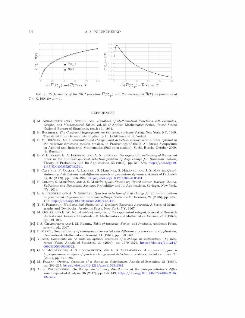
We conclude with an illustration of the obtained result, viz. (15), at work. Specifi-cally, we wrote a Mathematica script that numerically evaluates the delay risk C(τ∗AT

)

ON OPTIMALITY OF THE SHIRYAEV–ROBERTS–POLLAK PROCEDURE 13

and the lowerbound B(T ) via formulae (17) and (34), respectively. The script allowsto compute C(τ∗AT

) and B(T ) to within any desired accuracy, although each ad-ditional decimal place of accuracy clearly comes at the “price” of slower speed ofcomputation. As a reasonable compromise, we went with ten decimal places, whichis more than sufficient for our purposes, and yet, on an average laptop, the amountof time it takes the script to finish is on the order of seconds. The value of |µ| > 0is a factor as well: the computational time is lesser the higher the value of |µ|. Thismakes sense because the pre- and post-change hypotheses are harder to differentiatebetween when |µ| is small. We experimented with two scenarios: µ = 1/2, which is arelatively small (harder to detect) change, and µ = 1, which is a more contrast (easierto detect) change. For each of the two values of µ the experiment consisted in varyingthe ARL to false alarm level T from 1 up through 100 in increments of 1, and usingthe script to compute C(τ∗AT

) and B(T ) for each T . The threshold AT > 0 required

for the evaluation of C(τ∗AT) was recovered numerically from equation (27) using the

high-order approximations obtained in [15]. All of the obtained experimental resultsare shown in Figures 1 and 2. Specifically, either figure is a pair of graphs arrangedside by side: one showing C(τ∗AT

) and B(T ) together in one plot, and one showing

the corresponding difference C(τ∗AT) − B(T ) in a separate plot—all as functions of

T ∈ [1, 100]. Figure 1 corresponds to µ = 1/2, and Figure 2 corresponds to µ = 1.

0 20 40 60 80 1000

2

4

6

8

10

12

14

(a) C(τ∗AT) and B(T ) vs. T

0 20 40 60 80 1000.20

0.25

0.30

0.35

0.40

0.45

0.50

0.55

0.60

(b) C(τ∗AT)−B(T ) vs. T

Fig. 1. Performance of the SRP procedure C(τ∗AT) and the lowerbound B(T ) as functions of

T ∈ [0, 100] for µ = 1/2.

A visual inspection of the figures suggests two conclusions to draw. First, itis fairly evident that C(τ∗AT

) does, in fact, converge to B(T ) from above. This isexactly what one would expect in view of (15). Second, the convergence is slower forµ = 1/2 than for µ = 1, which is also an expected result, because fainter changes aremore difficult to detect, so that C(τ∗AT

) and B(T ) are both larger, and the differencebetween the two is more pronounced as well. We also experimented with ramping upthe ARL to false alarm level T to as high as 10, 000 and setting µ as low as 1/10,and obtained sufficiently convincing numerical evidence that C(τ∗AT

) does eventually

“blend in” with B(T ), even if µ is small.

Acknowledgments. The author is thankful to Dr. E.V. Burnaev of the Kharke-vich Institute for Information Transmission Problems, Russian Academy of Sciences,Moscow, Russia, and to Prof. A.N. Shiryaev of the Steklov Mathematical Institute,Russian Academy of Sciences, Moscow, Russia, for the interest and attention to thiswork.

14 A. S. POLUNCHENKO

0 20 40 60 80 1000

1

2

3

4

5

6

(a) C(τ∗AT) and B(T ) vs. T

0 20 40 60 80 1000.05

0.06

0.07

0.08

0.09

0.1

0.11

0.12

0.13

0.14

(b) C(τ∗AT)−B(T ) vs. T

Fig. 2. Performance of the SRP procedure C(τ∗AT) and the lowerbound B(T ) as functions of

T ∈ [0, 100] for µ = 1.

REFERENCES

[1] M. Abramowitz and I. Stegun, eds., Handbook of Mathematical Functions with Formulas,Graphs, and Mathematical Tables, vol. 55 of Applied Mathematics Series, United StatesNational Bureau of Standards, tenth ed., 1964.

[2] H. Buchholz, The Confluent Hypergeometric Function, Springer-Verlag, New York, NY, 1969.Translated from German into English by H. Lichtblau and K. Wetzel.

[3] E. V. Burnaev, On a nonrandomized change-point detection method second-order optimal inthe minimax Brownian motion problem, in Proceedings of the X All-Russia Symposiumon Applied and Industrial Mathematics (Fall open session), Sochi, Russia, October 2009.(in Russian).

[4] E. V. Burnaev, E. A. Feinberg, and A. N. Shiryaev, On asymptotic optimality of the secondorder in the minimax quickest detection problem of drift change for Brownian motion,Theory of Probability and Its Applications, 53 (2009), pp. 519–536, https://doi.org/10.1137/S0040585X97983791.

[5] P. Cattiaux, P. Collet, A. Lambert, S. Martınez, S. Meleard, and J. S. Martın, Quasi-stationary distributions and diffusion models in population dynamics, Annals of Probabil-ity, 37 (2009), pp. 1926–1969, https://doi.org/10.1214/09-AOP451.

[6] P. Collet, S. Martınez, and J. S. Martın, Quasi-Stationary Distributions: Markov Chains,Diffusions and Dynamical Systems, Probability and Its Applications, Springer, New York,NY, 2013.

[7] E. A. Feinberg and A. N. Shiryaev, Quickest detection of drift change for Brownian motionin generalized Bayesian and minimax settings, Statistics & Decisions, 24 (2006), pp. 445–470, https://doi.org/10.1524/stnd.2006.24.4.445.

[8] T. S. Ferguson, Mathematical Statistics: A Decision Theoretic Approach, A Series of Mono-graphs and Textbooks, Academic Press, New York, NY, 1967.

[9] M. Geller and E. W. Ng, A table of integrals of the exponential integral, Journal of Researchthe National Bureau af Standards—B. Mathematics and Mathematical Science, 73B (1969),pp. 191–210.

[10] I. S. Gradshteyn and I. M. Ryzhik, Table of Integrals, Series, and Products, Academic Press,seventh ed., 2007.

[11] P. Mandl, Spectral theory of semi-groups connected with diffusion processes and its application,Czechoslovak Mathematical Journal, 11 (1961), pp. 558–569.

[12] Y. Mei, Comments on “A note on optimal detection of a change in distribution,” by Ben-jamin Yakir, Annals of Statistics, 34 (2006), pp. 1570–1576, https://doi.org/10.1214/009053606000000362.

[13] G. V. Moustakides, A. S. Polunchenko, and A. G. Tartakovsky, A numerical approachto performance analysis of quickest change-point detection procedures, Statistica Sinica, 21(2011), pp. 571–596.

[14] M. Pollak, Optimal detection of a change in distribution, Annals of Statistics, 13 (1985),pp. 206–227, https://doi.org/10.1214/aos/1176346587.

[15] A. S. Polunchenko, On the quasi-stationary distribution of the Shiryaev–Roberts diffu-sion, Sequential Analysis, 36 (2017), pp. 126–149, https://doi.org/10.1080/07474946.2016.1275512.

ON OPTIMALITY OF THE SHIRYAEV–ROBERTS–POLLAK PROCEDURE 15

[16] A. S. Polunchenko and A. G. Tartakovsky, On optimality of the Shiryaev–Roberts proce-dure for detecting a change in distribution, Annals of Statistics, 38 (2010), pp. 3445–3457,https://doi.org/10.1214/09-AOS775.

[17] A. S. Polunchenko and A. G. Tartakovsky, State-of-the-art in sequential change-pointdetection, Methodology and Computing in Applied Probability, 14 (2012), pp. 649–684,https://doi.org/10.1007/s11009-011-9256-5.

[18] S. W. Roberts, A comparison of some control chart procedures, Technometrics, 8 (1966),pp. 411–430.

[19] A. N. Shiryaev, The problem of the most rapid detection of a disturbance in a stationaryprocess, Soviet Mathematics—Doklady, 2 (1961), pp. 795–799. Translation from Dokl.Akad. Nauk SSSR 138:1039–1042, 1961.

[20] A. N. Shiryaev, On optimum methods in quickest detection problems, Theory of Probabilityand Its Applications, 8 (1963), pp. 22–46, https://doi.org/10.1137/1108002.

[21] A. N. Shiryaev, Optimal Stopping Rules, Springer-Verlag, New York, NY, 1978.[22] A. N. Shiryaev, Quickest detection problems in the technical analysis of the financial data,

in Mathematical Finance—Bachelier Congress 2000, H. Geman, D. Madan, S. R. Pliska,and T. Vorst, eds., Springer Finance, Springer Berlin Heidelberg, 2002, pp. 487–521, https://doi.org/10.1007/978-3-662-12429-1 22.

[23] A. N. Shiryaev, From “disorder” to nonlinear filtering and martingale theory, in MathematicalEvents of the Twentieth Century, A. A. Bolibruch, Y. S. Osipov, and Y. G. Sinai, eds.,Springer Berlin Heidelberg, 2006, pp. 371–397, https://doi.org/10.1007/3-540-29462-7 18.

[24] A. N. Shiryaev, Probabilistic–Statistical Methods in Decision Theory, Yandex School of DataAnalysis Lecture Notes, MCCME, Moscow, Russia, 2011. (in Russian).

[25] A. N. Shiryaev, Stochastic Change-Point Detection Problems, MCCME, Moscow, Russia,2017. (in Russian).

[26] A. N. Shiryaev and P. Y. Zryumov, On the linear and nonlinear generalized Bayesian disor-der problem (discrete time case), in Optimality and Risk—Modern Trends in MathematicalFinance, F. Delbaen, M. Rasonyi, and C. Stricker, eds., Springer Berlin Heidelberg, 2010,pp. 227–236, https://doi.org/10.1007/978-3-642-02608-9 12.

[27] L. J. Slater, Confluent Hypergeometric Functions, Cambridge University Press, Cambirdge,UK, 1960.

[28] A. Tartakovsky, I. Nikiforov, and M. Basseville, Sequential Analysis: Hypothesis Testingand Changepoint Detection, vol. 166 of Monographs on Statistics and Applied Probability,CRC Press, Boca Raton, FL, 2014.

[29] A. G. Tartakovsky and G. V. Moustakides, State-of-the-art in Bayesian change-point detection, Sequential Analysis, 29 (2010), pp. 125–145, https://doi.org/10.1080/07474941003740997.

[30] A. G. Tartakovsky, M. Pollak, and A. S. Polunchenko, Third-order asymptotic op-timality of the Generalized Shiryaev–Roberts changepoint detection procedures, Theoryof Probability and Its Applications, 56 (2012), pp. 457–484, https://doi.org/10.1137/S0040585X97985534.

[31] A. G. Tartakovsky and A. S. Polunchenko, Minimax optimality of the Shiryaev–Robertsprocedure, in Proceedings of the 5th International Workshop in Applied Probability, Uni-versidad Carlos III de Madrid, Spain, July 2010.

[32] E. T. Whittaker, An expression of certain known functions as generalized hypergeometricfunctions, Bulletin of the American Mathematical Society, 10 (1904), pp. 125–134.

[33] E. T. Whittaker and G. N. Watson, A Course of Modern Analysis, Cambridge UniversityPress, Cambridge, UK, fourth ed., 1927.

[34] B. Yakir, A note on optimal detection of a change in distribution, Annals of Statistics, 25(1997), pp. 2117–2126, https://doi.org/10.1214/aos/1069362390.