Keynesian Dynamics and the Wage-Price Spiral. Estimating a

Keynesian Dynamics and the Wage-Price Spiral.Estimating a Baseline Disequilibrium Approach∗

Pu Chen

Faculty of EconomicsBielefeld University, Bielefeld

Germany

Carl Chiarella

School of Finance and EconomicsUniversity of Technology, Sydney

Australia

Peter Flaschel

Faculty of Economics

Bielefeld UniversityGermany

Willi Semmler

Faculty of Economics

Bielefeld University, BielefeldGermany

May 28, 2004

Abstract:We reformulate the baseline disequilibrium AS-AD model of Asada, Chen, Chiarella

and Flaschel (2004) to make it applicable for empirical estimation. The model now ex-hibits a Taylor interest rate rule in the place of an LM curve, a dynamic IS curve anddynamic employment adjustment. It is based on sticky wages and prices, perfect foresightof current inflation rates and adaptive expectations concerning the inflation climate inwhich the economy is operating. The implied nonlinear 5D model of real markets dise-quilibrium dynamics avoids striking anomalies of the Neoclassical synthesis (Stage I). Itexhibits Keynesian feedback structures with asymptotic stability of its steady state forlow adjustment speeds and with cyclical loss of stability – by way of Hopf bifurcations –when certain adjustment speeds are made sufficiently large.

In the second part we estimated the equations of the model to study its stabilityfeatures from the empirical point of view with respect to the feedback chains it exhibits.Based on these estimates we also study to which extent a stronger Blanchard / Katz errorcorrection mechanism, more pronounced interest rate feedback rules or downward wagerigidity can stabilize the dynamics in the large when the steady state is found to be locallyrepelling. The achievements of this baseline disequilibrium AS-AD model, its Keynesianfeedback channels and our empirical findings can be usefully contrasted with those of themicrofounded, but in scope more limited now fashionable New Keynesian alternative (theNeoclassical Synthesis, Stage II).

———————Keywords: DAS-DAD growth, wage and price Phillips curves, estimation, adverse realwage adjustment, (in)stability, persistent business cycles, monetary policy rules.

JEL CLASSIFICATION SYSTEM: E24, E31, E32.

∗Preliminary version. Please do not quote without permission from the authors.

1

1 Introduction

In this paper we reformulate and extend the standard AS-AD growth dynamics of theNeoclassical Synthesis (Stage I) with its traditional microfoundations, as it is for exampletreated in detail in Sargent (1987, Ch.5). Our reformulation, based on our earlier pre-sentation and analysis of a DAS-AD alternative to the neoclassical AS-AD framework,see Asada, Chen, Chiarella, Flaschel (2004), now replaces their LM curve with a Taylorinterest rate policy rule, as in the New Keynesian approaches. The model, as well asits predecessor, exhibits sticky wages as well as sticky prices, underutilized labor as wellas capital stock, myopic perfect foresight of current wage and price inflation rates andadaptively formed medium run expectations concerning the inflation climate in whichthe economy is operating. Moreover we now employ a dynamic IS-equation in the placeof the static one of Asada, Chen, Chiarella, Flaschel (2004) and will also make use of adynamic form of Okun’s law to a certain extent. The resulting nonlinear 5D model oflabor and goods market disequilibrium dynamics (with a Taylor type treatment of thefinancial part of the economy) avoids the striking anomalies of the conventional AS-ADmodel of the Neoclassical synthesis under myopic perfect foresight, stage I.1 Instead itexhibits Keynesian feedback dynamics proper with in particular asymptotic stability ofits unique interior steady state solution for low adjustment speeds of wages, prices, andexpectations among others. The loss of stability occurs cyclically, by way of Hopf bifur-cations, when some of these adjustment speeds are made sufficiently large, even leadingeventually to purely explosive dynamics sooner or later. This latter fact – if it occurs– implies the need to look for appropriate extrinsic nonlinearities that can bound thedynamics in an economically meaningful domain, such as downward rigidity of wagesand prices and the like, if the economy departs too much from its steady state position.

Locally we thus obtain and can prove the existence of in general damped, persistent orexplosive fluctuations in the real and the nominal part of the dynamics, in the rates ofcapacity utilization of both labor and capital, and of wage and price inflation rates whichhere induce interest rate adjustments by the monetary authority that attempt to stabilizethe observed output and price level fluctuations. Our modification and extension oftraditional AS-AD growth dynamics, as investigated from the orthodox point of view inSargent (1987), thus provides us with a Keynesian theory of the business cycle, includinga modern approach to monetary policy. This is even true in the case of myopic perfectforesight, where the structure of the traditional approach radically dichotomizes intoindependent classical supply-side and real dynamics – that cannot be influenced bymonetary policy – and a subsequently determined inflation dynamics, that are purelyexplosive if the price level is taken as a predetermined variable, a situation that forcedconvergence by an inconsistent application of the jump-variable technique2 in Sargent(1987,ch.5), see again Asada, Chen, Chiarella and Flaschel (2004) for details. In ournew type of Keynesian labor and goods market dynamics we however can treat myopicperfect foresight of both firms and wage earners without the need for the methodologyof the rational expectations approach to unstable saddlepoint dynamics.

1These anomalies include in particular saddle point dynamics that imply instability unless somepoorly motivated jumps – and indeed flawed – are imposed on certain variables, here on both the priceand the wage level, see Asada, Chen, Chiarella and Flaschel (2004) for details.

2since the nominal wage is transformed into a non-predetermined variable there.

2

From the global perspective, if our model loses asymptotic stability for higher adjustmentspeeds, in the present framework specifically of prices and the inflationary climate, purelyexplosive behavior is the generally observed outcome, as is easily checked by means ofnumerical simulations. The considered so far only intrinsically nonlinear model typetherefore cannot be considered as being complete in such circumstances, since somemechanism is then required to bound the fluctuations to economically viable regions.Downward money wage rigidity is the mechanism we have often used for this purposeand which we will use here again, see the numerical investigations in Asada, Chiarella,Flaschel and Hung (2004). Extended in this way, by simply excluding deflation (tosome extent) for m occurring, we obtain and study a baseline model of the DAS-DADvariety with a rich set of stability implications and with various types of business cyclefluctuations that it can generate endogenously or by adding stochastic shocks to theconsidered dynamics.

The dynamic outcomes of this baseline disequilibrium AS-AD or DAS-DAD model canbe usefully contrasted with those of the currently fashionable New Keynesian alternative(the Neoclassical Synthesis, stage II) that in our view is more limited in scope, at leastas far as the treatment of interacting Keynesian feedback mechanisms and the therebyimplied dynamic possibilities are concerned. This comparison reveals in particular thatone does not always end up with the typical (in our view strange) dynamics of rationalexpectation models, due to certain types of forward looking behavior, if such behavior iscoupled with plausible backward looking behavior for the medium-run evolution of theeconomy. This basic insight is now also stressed in New Keynesian approaches due tothe complete empirical failure of their New Phillips curve.

Our dual Phillips curves approach to the wage-price spiral indeed performs quite well,when estimated empirically, as we shall show in this paper,3 in particular does notgive rise to the situation observed for the New (Keynesian) Phillips curve, found to becompletely at odds with the facts in the literature 4. In our approach standard Keynesianfeedback mechanisms are coupled with a wage-price spiral having a considerable degreeof inertia, with the result that these feedback mechanisms work – as is known frompartial analysis – in their interaction with the added wage and price level dynamics.

The present paper therefore intends to provide a proper baseline model of the KeynesianDAS-DAD variety, not plagued by the theoretical anomalies of the traditional AS-ADmodel and the empirical anomalies of the New Keynesian approach. It does so on thebasis of the fully specified DAS-AD growth dynamics of Asada, Chen, Chiarella andFlaschel (2004), by transforming this dynamics into a reduced DAS-DAD form that canbe estimated empirically. It discusses the feedback structure of this reduced form andits stability implications, first on a general level and then on the level of the sign restric-tions obtained from empirical estimates of the five laws of motion of the dynamics. Theseestimates also allow us to show asymptotic stability for the estimated parameter sizesand to determine stability boundaries (with respect to price flexibility and the speed of

3See also Flaschel and Krolzig (2004), Flaschel, Kauermann and Semmler (2004) and Chen andFlaschel (2004).

4In this connection, see for example Mankiw (2001) and with much more emphasis Eller and Gordon(2003), whereas Gali, Gertler and Lopez-Salido (2003) argue in favor of a hybrid form of the NewPhillips Curve.

3

adjustment of the inflationary climate) where the need for further (behavioral) nonlin-earities therefore becomes established, to be investigated and discussed in a companionpaper to the present one (Asada, Chiarella, Flaschel and Hung, 2004).

Section 2 presents our reformulation of the baseline Keynesian DAS-AD growth dynamicsof Asada, Chen, Chiarella and Flaschel (2004) as a DAS-DAD growth dynamics in orderto make this model applicable to empirical estimation. Section 3 considers the feedbackchains of the reformulated model and derives cases of local asymptotic stability andof loss of stability by way of Hopf-bifurcations. In section 4 we estimate the modelto find out sign restrictions and which type of feedback mechanisms may apply to theUS-economy after World War II. Section 5 then investigates again the stability of thedynamics on the basis of these sign restrictions and determines stability boundaries withrespect to the adjustment speed of prices and the inflationary climate variable. Section 6concludes and considers briefly behavioral assumptions that may provide global stabilityto the economy in the cases where the steady state is surrounded by centrifugal forces.We there also discuss in which way the resulting persistent fluctuations will be influencedthrough a stronger conduct of interest rate policy rules.

2 Keynesian disequilibrium dynamics: Empirically

oriented reformulation of a baseline model

In this section we reformulate the theoretical disequilibrium model of AS-AD growth ofAsada, Chen, Chiarella and Flaschel (2004) in order to make it applicable for empiricalestimation and for the study of the role of contemporary interest rate policy rules. Wethus dismiss the LM curve of the original approach and replace it now by a Taylorinterest rate policy rule and now also use dynamic IS as well as employment equationsin the place of static ones of the original approach, where with respect to the former thedependence of consumption and investment on income distribution now only appearsin aggregated or reduced type format. We furthermore now use Blanchard and Katz(2000) type error correction terms both in the wage and the price Phillips curve thatgive income shares a role to play in wage as well as in price dynamics. Finally, we willadd inflationary inertia to a world of myopic perfect foresight through the inclusion ofa medium-run variable, the inflationary climate in which the economy is operating, andits role in the wage and price dynamics of the considered economy.

We start from the observation that a Keynesian model of aggregate demand fluctuationsshould (independently of whether justification can be found for this in Keynes’ GeneralTheory) allow for under- (or over-)utilized labor as well as capital in order to be generalenough from the descriptive point of view. As Barro (1994) for example observes, IS-LM is (or should be) based on imperfectly flexible wages and prices and thus on theconsideration of wage as well as price Phillips Curves. This is precisely what we will doin the following, augmented by the observation that medium-run aspects count both inwage and price adjustments, here still formulated in simple terms by the introductionof the concept of an inflation climate. This economic climate term is based on pastobservation, while we have model-consistent expectations with respect to short-run wage

4

and price inflation. The modification of the traditional AS-AD model that we shallintroduce thus treats expectations in a hybrid way, myopic perfect foresight of the currentrates of wage and price inflation on the one hand and an adaptive updating of aneconomic climate expression with exponential or other weighting scheme on the otherhand.

We assume two Phillips Curves or PC’s in the place of only one. In this way we candiscuss wage and price dynamics separately from each other, in their structural forms,both based on their own measure of demand pressure, namely V l − V l, V c − V c, inthe market for labor and for goods, respectively. We here denote by V l the rate ofemployment on the labor market and by V l the NAIRU-level of this rate, and similarly byV c the rate of capacity utilization of the capital stock and V c the normal rate of capacityutilization of firms. These demand pressure influences on wage and price dynamics, or onthe formation of wage and price inflation, w, p, are here both augmented by a weightedaverage of cost-pressure terms based on forward looking myopic perfect foresight and abackward looking measure of the prevailing inflationary climate, symbolized by πm. Costpressure perceived by workers is a weighted average of the currently evolving rate of priceinflation p and a medium-run concept of price inflation, πm, the inflationary climate inwhich the economy is operating, which is based on past observations. Similarly, costpressure perceived by firms is given by a weighted average of the currently evolving(perfectly foreseen) rate of wage inflation w and again the measure of the inflationaryclimate in which the current state of the economy is embedded.

We thereby arrive at the following two Phillips Curves for wage and price inflation,which in this core version of Keynesian AS-AD dynamics are – qualitatively seen – stillformulated in a fairly symmetric way.5 We stress that we have included forward-lookingbehavior here, without the (later) need for the jump variable technique of the rationalexpectations school.

Structural form of the wage-price dynamics:

w = βw1(Vl − V l) − βw2(ω − ωo) + κwp + (1 − κw)πm,

p = βp1(Vc − V c) + βp2(ω − ωo) + κpw + (1 − κp)π

m.

Inflationary expectations over the medium run, πm, i.e., the inflationary climate in whichcurrent inflation is operating, may be adaptively following the actual rate of inflation(by use of some linear or exponential weighting scheme), may be based on a rollingsample (with hump-shaped weighting schemes), or on other possibilities for updatingexpectations. For simplicity of the exposition we shall make use of the conventionaltheoretical expression of an adaptive expectations mechanism:

5With respect to empirical estimation we could also consider the role of labor productivity growth,which we here assume to be zero to ease the presentation of the model. This role is found to be of secondorder only in the empirical estimates of the considered wage and price Phillips curves, as far as trendterms in wage inflation are concerned. And with respect to the distinction between real wages, unitwage costs and the wage share we shall detrend the corresponding time series such that the followingtypes of PC’s can still be applied. empirically, we therefore concentrate on the cyclical features of themodel by the formulation of the structural equations of the model and the choice of detrended timeseries.

5

πm = βπm(p − πm)

in the presentation of the full model below. Besides demand pressure we thus use (as costpressure expressions) in the two PC’s weighted averages of this economic climate andthe (foreseen) relevant temporary cost pressure term for future wage and price setting.In this way we get two PC’s with very analogous building blocks, which despite theirtraditional outlook will have a variety of interesting and novel implications. Somewhatsimplified versions of these two Phillips curves have been estimated for the US-economyin various ways in Flaschel and Krolzig (2004), Flaschel, Kauermann and Semmler (2004)and Chen and Flaschel and Chen (2004) and found to represent a significant improvementover single reduced-form Phillips curves, with in fact wage flexibility being greater thanprice flexibility with respect to their demand pressure item in the market for goodsand for labor, respectively. Note that such a finding is not possible in the conventionalframework of a single reduced-form Phillips curve.

We have added here to these earlier studies Blanchard and Katz type error correctionmechanisms (the second β terms in each equation) not only in the wage inflation equa-tion, but also in the price inflation equation. The minus sign in front of βw2 is motivatedas in the article of Blanchard and Katz (2000), see also Flaschel and Krolzig (2004) inthis regard, while the plus sign in front of βp2 simply represents a second measure ofcost pressure, in addition to the weighted average of inflation rates shown thereafter. Tosimplify steady state calculations we measure these error correction terms in deviationfrom their steady state values.

Note that for our current version, the inflationary climate variable does not matterfor the evolution of the real wage ω = w/p , the law of motion of which is given by(κ = 1/(1 − κwκp)):

ω = κ[(1 − κp)(βw1(Vl − V l) − βw2(ω − ωo)) − (1 − κw)(βp1(V

c − V c) + βp2(ω − ωo))]

This follows easily from the following obviously equivalent representation of the abovetwo PC’s:

w − πm = βw1(Vl − V l) − βw2(ω − ωo) + κw(p − πm),

p − πm = βp1(Vc − V c) + βp2(ω − ωo)) + κp(w − πm),

by solving for the variables w − πm and p − πm. It also implies the two across-marketsor reduced form PC’s given by:

p = κ[βp1(Vc − V c) + βp2(ω − ωo) + κp(βw1(V

l − V l) − βw2(ω − ωo))] + πm,

w = κ[βw1(Vl − V l) − βw2(ω − ωo)) + κw(βp1(V

c − V c) + βp2(ω − ωo))] + πm,

which represent a considerable generalization of the conventional view of a single-marketprice PC with only one measure of demand pressure, the one in the labor market.

The remaining laws of motion of the private sector of the model are as follows:

V c = −αV c(V c − V c) ± αω(ω − ωo) − αr((r − p) − (ro − π))

V l = βV l1(V c − V c) − βV l

2(ω − ωo) + βV l

3V c

6

The first law of motion is of the type of a dynamic IS-equation, see also Rudebuschand Svensson (1999) in this regard, here expressed in terms of the growth rate of therate of capacity utilization of firms and linearized around the steady state of the model.It reflects the dependence of excess goods demand on aggregate (income) supply andthus on the rate of capacity utilization by assuming a negative, i.e., stable dynamicmultiplier relationship in this respect, it shows the joint dependence of consumptionand investment on the real wage (which in the aggregate allows for positive or negativesigns before αω depending on whether consumption or investment is more responsive toreal wage changes) and shows finally the negative influence of the real rate of intereston the evolution of economic activity. Note here that we have generalized this law ofmotion in comparison to the original baseline model of Asada, Chen, Chiarella andFlaschel (2004), since we now allow for the possibility that also consumption, not onlyinvestment, depends on income distribution as measured by the real wage.

In the second law of motion, for the rate of employment, we assume that the employmentpolicy of firms follows their rate of capacity utilization (and the thereby implied rate ofover- or underemployment of the employed workforce) with a lag (measured by 1/βV l

1).

Employment is thus assumed to adjust to the level of current activity in delayed formwhich is a reasonable assumption from the empirical point of view. We also include(via the parameter βV l

2) an influence of income distribution on the rate of change of the

employment rate. The last term finally, βV l2V c, is added to take account of the possibility

that Okun’s is to be formulated in level form rather than by a law of motion, since this

term is equivalent to the use of const (V c)β

V l2 , the form of Okun’s law in which this law

was originally specified by Okun himself.

The above two laws of motion therefore summarize the static IS-curve and the employ-ment this curve implies of the paper of Asada, Chen, Chiarella and Flaschel (2004) in adynamic form. They also reflect the there assumed influence of smooth factor substitu-tion in production and the measurement of the potential output this implied in Asada,Chen, Chiarella and Flaschel (2004) in an indirect form, as another positive influenceof the real wage on the rate of capacity utilization and its rate of change. This helps toavoid the estimation of separate equations for consumption and investment C, I and forpotential output Y p as they were discussed and used in detail in Asada, Chen, Chiarellaand Flaschel (2004).

Finally, we have no longer to employ a law of motion for real balances as still was the casein Asada, Chen, Chiarella and Flaschel (2004). Money supply is now accommodating tothe interest rate policy pursued by the central bank and thus does not feedback into thecore laws of motion of the model. As interest rate policy we here assume the followingtype of Taylor rule:

r = −γr(r − ro) + γp(p − π) + γV c(V c − V c) + γω(ω − ωo)

Note that we allow for interest rate smoothing in this rule. Furthermore, the actual(perfectly foreseen) rate of inflation p is used to measure the inflation gap with respectto the inflation target π of the central bank. There is next a positive influence of theoutput gap in this law of motion for the rate of interest, here measured by the rateof capacity utilization of firms. Note finally that we have included a new kind of gap

7

into the above Taylor rule, the real wage gap, since we have in our model a dependenceof aggregate demand on income distribution and the real wage. The state of incomedistribution matters for the dynamics of our model and thus should also play a role inthe decisions of the central bank. All of the employed gaps are measured relative to thesteady state of the model, in order to allow for an interest rate policy that is consistentwith balanced growth.

We note that the steady state of the considered Keynesian dynamics is basically the sameas the one considered in Asada, Chen, Chiarella and Flaschel (2004), with εo = 0, V c

o =V c, V l

o = V l, πmo = π. The values of ωo, ro are in principle determined as in Asada, Chen,

Chiarella and Flaschel (2004), but are here just assumed as given, underlying the linearapproximation of the present model around the steady state of the original framework(when adjusted to the considered modifications of the baseline model).

The steady state of the dynamics is locally asymptotically stable under certain sluggish-ness conditions that are reasonable from a Keynesian perspective, loses its asymptoticstability by way of cycles (by way of so-called Hopf-bifurcations) if the system becomestoo flexible, and becomes sooner or later globally unstable if (generally speaking) ad-justment speeds become too high, as we shall show below. If the model is subject toexplosive forces, it requires extrinsic nonlinearities in economic behavior – like down-ward wage rigidity – to come into being at least far off the steady state in order tobound the dynamics to an economically meaningful domain in the considered 5D statespace. Asada, Chiarella, Flaschel and Hung (2004) provide details for such an approachwith extrinsically motivated nonlinearities and undertake its detailed numerical investi-gation. In sum, therefore, our dynamic AS-AD growth model here and there will exhibita variety of features that are much more in line with a Keynesian understanding ofthe characteristics of the trade cycle than is the case for the conventional modelling ofAS-AD growth dynamics or its reformulation by the New Keynesians.

Taken together the model of this section consists of the five laws of motion:

V c = −αV c(V c − V c) ± αω(ω − ωo) − αr((r − p) − (ro − π)) (1)


2(ω − ωo) + βV l

3V c (2)

r = −γr(r − ro) + γp(p − π) + γV c(V c − V c) + γω(ω − ωo) (3)

ω = κ[(1 − κp)(βw1(Vl − V l) − βw2(ω − ωo)) − (1 − κw)(βp1(V

c − V c) + βp2(ω − ωo))]

(4)

πm = βπm(p − πm) or πm(t) = πm(to)e−βπm(t−to) + βπm

∫ t

to

eβπm(t−s)p(s)ds (5)

where the following reduced form expression for the price inflation rate

p = κ[βp1(Vc − V c) + βp2(ω − ωo) + κp(βw1(V

l − V l) − βw2(ω − ωo))] + πm

has to be inserted into the third and fifth equation in order to get an autonomous systemof differential equations in the state variables: capacity utilization V c, the rate of em-ployment V l, the rate of interest r, the real wage rate ω and the inflationary climate πm.

8

This modification and extension of the baseline disequilibrium AS-AD model of Asada,Chen, Chiarella and Flaschel (2004) in particular goes beyond this earlier approach asit now also allows for positive effects of real wage changes on aggregate demand, not yetpresent in the AD component of our original modification of the conventional AS-ADdynamics.

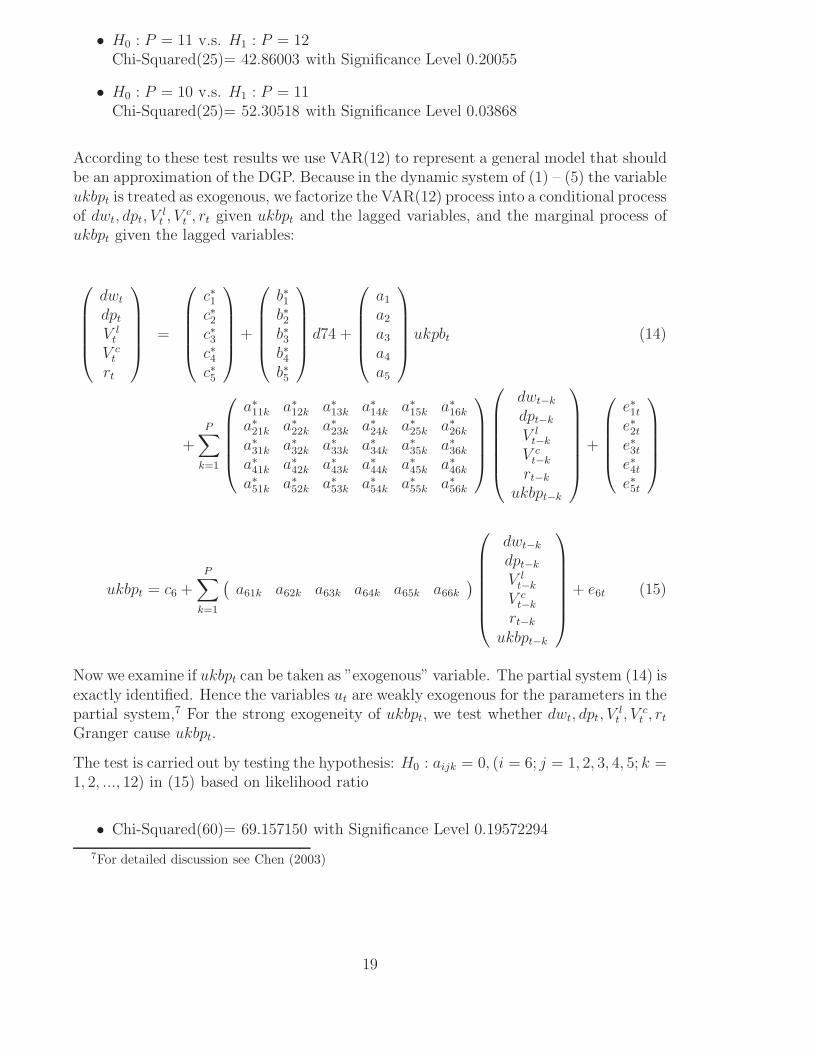
The above model – though not microfounded by making the representative householdassumption – is microfounded in the way Keynesian theory was microfounded afterPatinkin and it also makes use of recent approaches, to labor market dynamics as inBlanchard and Katz (2000). With respect to empirically relevant restructuring of thetheoretical framework it is as pragmatic as for example the approach employed by Rude-busch and Svensson (1999). By and large we therefore believe that it represents a workingalternative to the New Keynesian approach, in particular when the critique of the latterapproach is taken into account. It overcomes the weaknesses and the logical inconsisten-cies of the Neoclassical synthesis, stage I, and it does so in a minimal way from a maturetraditional Keynesian perspective (that is not really ’New’). It preserves the problematicnature of the real rate of interest channel, where the stabilizing Keynes effect (or the in-terest rate policy of the central bank) is interacting with the destabilizing, expectationsdriven Mundell effect. And it preserves the real wage effect of the Neoclassical synthesis,stage I, where – due to a negative dependence of aggregate demand on the real wage– we have that price flexibility is destabilizing, while wage flexibility is not. This realwage channel is not a topic in the New Keynesian approach, due to the specific form ofwage-price dynamics there considered, see for example Woodford (2003, p.225), and it issummarized in the figure 1 for the situation where investment dominates consumptionwith respect to real wage changes. In the opposite case, the situations considered willbe reversed with respect to their stability implications.

AssetMarkets:

DepressedGoods Markets

DepressedLabor Markets

wages

prices

Normal Rose Effect (example):

interest rates

investment

aggregate demand

Recovery!

Recovery!

real wages

consumption

?

AssetMarkets:

DepressedGoods Markets

DepressedLabor Markets

wages

prices

Adverse Rose Effect (example):

interest rates

investment

aggregate demand

Further

Further

real wages

consumption

?

Figure 1: Rose effects: The real wage channel of Keynesian macrodynamics .

The feedback channels just discussed will be the focus of interest in the now following

9

stability analysis of the DAS-DAD dynamics.

We note that the rate of employment, if above the NAIRU level, may also act negativelyon the growth rate of capacity utilization, i.e., on the first law of motion, when theKaleckian view of the political business cycle (bosses do not like full employment) istaken into account in addition. There may of course also be derivative influences (timederivatives of the considered variables) added to the considered equations, which indeedshould have the same sign as the level influence, since they add to the impact of highlevels if the considered change is positive. Such extensions of the present dynamics musthere however be left for their future investigation.

We have employed reduced-form expressions in the above system of differential equationswhenever possible. We have thereby obtained a dynamical system in five state variablesthat is in a natural or intrinsic way nonlinear. We note however that there are manyitems that reappear in various equations or are similar to each other implying thatstability analysis can exploit a variety of linear dependencies in the calculation of theconditions for local asymptotic stability. This dynamical system will be investigatedin the next section in somewhat informal terms with respect to the stability assertionsit gives rise to. A rigorous proof of local asymptotic stability and its loss by way ofHopf bifurcations can be found in Asada, Chen, Chiarella and Flaschel (2004) for theoriginal baseline dynamic AS-AD form of the considered disequilibrium AS-AD growthdynamics. For the present model variant we shall supply more detailed stability proofsin Asada, Chiarella, Flaschel and Hung (2004) and also detailed numerical simulationsof the model.

3 Feedback-guided stability analysis

In this section we illustrate an important method to prove local asymptotic stability ofthe interior steady state of the dynamical system (1) – (5) through partial motivationsfrom the feedback chains that characterize this baseline model of Keynesian dynamics.Since the model is an extension of the standard AS-AD growth model we know fromthe literature that there is a real rate of interest effect typically involved, first analyzedby formal methods in Tobin (1975), see also Groth (1992). Instead of the stabilizingKeynes-effect, based on activity-reducing nominal interest rate increases following pricelevel increases, we have here a direct steering of economic activity by the interest ratepolicy of the central bank. Secondly, if the correctly expected short-run real rate ofinterest is driving investment and consumption decisions (increases leading to decreasedaggregate demand), there is the activity stimulating (partial) effect of increases in therate of inflation that may lead to accelerating inflation under appropriate conditions.This is the so-called Mundell-effect that normally works opposite to the Keynes-effect,and through the same real rate of interest channel as this latter effect.

Due to our use of a Taylor rule in the place of the conventional LM curve, the Keynes-effect is here exploited in a more direct way towards a stabilization of the economy andit works the stronger the larger the parameters γp, γV c are chosen. The Mundell-effectby contrast is the stronger the faster the inflationary climate adjusts to the present level

10

of price inflation, since we have a positive influence of this climate variable both onprice as well as on wage inflation and from there on rates of employment of both capitaland labor. Excess profitability depends positively on the inflation rate and thus on theinflationary climate as the reduced-form price Phillips curve in particular shows.

There is a further important potentially (at least partially) destabilizing feedback mech-anism as the model is formulated. Excess profitability depends positively on the rate ofreturn on capital ρ and thus negatively on the real wage ω. We thus get – since con-sumption may also depend (positively) on the real wage – that real wage increases candepress or stimulate economic activity depending on whether investment or consumptionis dominating the outcome of real wage increases (we here neglect the stabilizing role ofthe Blanchard / Katz type error correction mechanisms). In the first case, we get fromthe reduced-form real wage dynamics:

ω = κ[(1 − κp)βw(V l − V l) − (1 − κw)βp(Vc − V c)].

that price flexibility should be bad for economic stability due to the minus sign infront of the parameter βp while the opposite should hold true for the parameter thatcharacterizes wage flexibility. This is a situation as it was already investigated in Rose(1967). It gives the reason for our statement that wage flexibility gives rise to normaland price flexibility to adverse Rose effects as far as real wage adjustments are concerned(if it is assumed – as in our baseline model – that only investment depends on the realwage). Besides real rate of interest effect, establishing opposing Keynes- and Mundell-effects, we thus have also another real adjustment process in the considered model wherenow wage and price flexibility are in opposition to each other, see Chiarella and Flaschel(2000) and Chiarella, Flaschel, Groh and Semmler (2000) for further discussion of theseas well as other feedback mechanisms in Keynesian growth dynamics. We stress againthat our DAS-AD growth dynamics – due to their origin in the baseline model of theNeoclassical Synthesis, stage I – allows for negative influence of real wage changes onaggregate demand solely, and thus only for cases of destabilizing wage level flexibility,but not price level flexibility. In the empirical estimation of the model we will indeedfind that this case seems to be the typical one in dynamic models of the AS-AD variety.

This adds to the description of the dynamical system (1) – (5) whose stability proper-ties are now to be investigated by means of varying adjustment speed parameters. Withthe feedback scenarios considered above in mind, we first observe that the inflationaryclimate can be frozen at its steady state value, here πm

o = π, if βπm = 0 is assumed. Thesystem thereby becomes 4D and it can indeed be further reduced to 3D if in additionαω = 0, γω = 0, βw2 = 0, βp2 = 0 is assumed, since this decouples the ω-dynamics fromthe remaining system V c, V l, r. We will consider the stability of these 3D subdynamics– and its subsequent extensions – in informal terms here only, reserving rigorous cal-culations to the alternative scenarios provided in Asada, Chiarella, Flaschel and Hung(2004). We nevertheless hope to show to the reader how one can proceed from low tohigh dimensional analysis in such stability investigations. This method has been alreadyapplied to various other, often much more complicated, dynamical systems, see Asada,Chiarella, Flaschel and Franke (2003) for a variety of typical examples.

Before we start with these stability investigations we establish that loss of stability canin general only occur in the considered dynamics by way of Hopf-bifurcations, since the

11

following proposition can be shown to hold true under mild – empirically plausible –parameter restrictions. Note that we assume for the dynamics of the employment ratethe simple rule V l = βV l(V c − V c) throughout this section.

Proposition 1:

Assume that the parameters γω, γr are chosen sufficiently small and that theparameters βw2 , βp2, κp fulfill βp2 > βw2κp. Then: The 5D determinant of theJacobian of the dynamics at the interior steady state is always negative insign.

Sketch of proof: We have for the sign structure in this Jacobian under the givenassumptions the following initial situation (we here assume as limiting situation γr =γω = 0):

J =

⎛⎜⎜⎜⎜⎝

± + − ± ++ 0 0 0 0+ + 0 0 +− + 0 − 0+ + 0 + −

⎞⎟⎟⎟⎟⎠ .

We note that the ambiguous sigh in the entry J11 in the above matrix is due to the factthat the real rate of interest is a decreasing function of the inflation rate which in turndepends positively on current rates of capacity utilization.

Using second row and the last row in its dependence on the partial derivatives of p wecan reduces this Jacobian to

J =

⎛⎜⎜⎜⎜⎝

0 0 − ± ++ 0 0 0 00 0 0 0 +0 + 0 − 00 + 0 + −

⎞⎟⎟⎟⎟⎠

without change in the sign of its determinant. In the same way we can now use thethird row to get another matrix without any change in the sign of the correspondingdeterminants

J =

⎛⎜⎜⎜⎜⎝

0 0 − ± 0+ 0 0 0 00 0 0 0 +0 + 0 − 00 + 0 + 0

⎞⎟⎟⎟⎟⎠

The last two columns can under the considered circumstance be further reduced to

J =

⎛⎜⎜⎜⎜⎝

0 0 − ± 0+ 0 0 0 00 0 0 0 +0 + 0 0 00 0 0 + 0

⎞⎟⎟⎟⎟⎠

12

which finally gives

J =

⎛⎜⎜⎜⎜⎝

0 0 − 0 0+ 0 0 0 00 0 0 0 +0 + 0 0 00 0 0 + 0

⎞⎟⎟⎟⎟⎠ .

This matrix is easily shown to exhibit a negative determinant which proves the propo-sition, also for all values of γr = γω which are chosen sufficiently small.

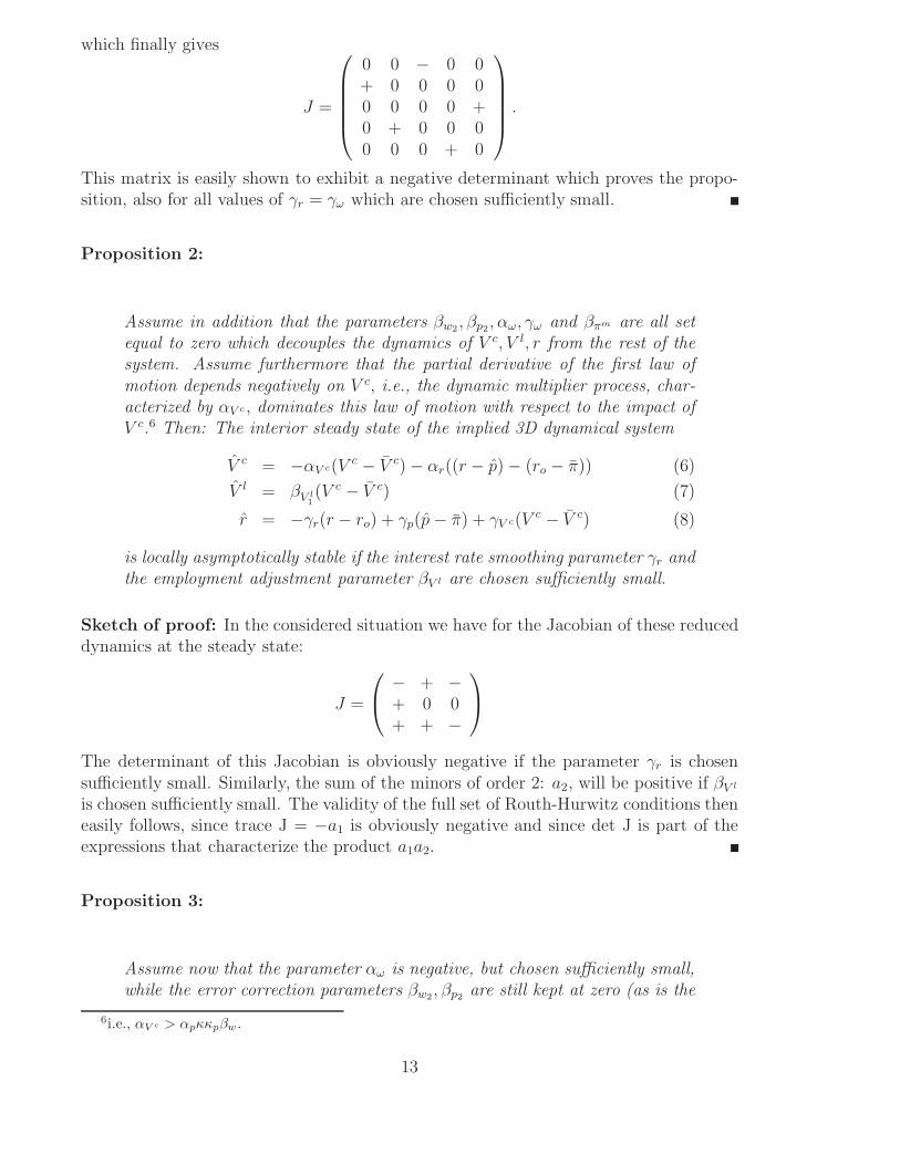
Proposition 2:

Assume in addition that the parameters βw2, βp2, αω, γω and βπm are all setequal to zero which decouples the dynamics of V c, V l, r from the rest of thesystem. Assume furthermore that the partial derivative of the first law ofmotion depends negatively on V c, i.e., the dynamic multiplier process, char-acterized by αV c , dominates this law of motion with respect to the impact ofV c.6 Then: The interior steady state of the implied 3D dynamical system

V c = −αV c(V c − V c) − αr((r − p) − (ro − π)) (6)

V l = βV l1(V c − V c) (7)

r = −γr(r − ro) + γp(p − π) + γV c(V c − V c) (8)

is locally asymptotically stable if the interest rate smoothing parameter γr andthe employment adjustment parameter βV l are chosen sufficiently small.

Sketch of proof: In the considered situation we have for the Jacobian of these reduceddynamics at the steady state:

J =

⎛⎝ − + −

+ 0 0+ + −

⎞⎠

The determinant of this Jacobian is obviously negative if the parameter γr is chosensufficiently small. Similarly, the sum of the minors of order 2: a2, will be positive if βV l

is chosen sufficiently small. The validity of the full set of Routh-Hurwitz conditions theneasily follows, since trace J = −a1 is obviously negative and since det J is part of theexpressions that characterize the product a1a2.

Proposition 3:

Assume now that the parameter αω is negative, but chosen sufficiently small,while the error correction parameters βw2, βp2 are still kept at zero (as is the

6i.e., αV c > αpκκpβw .

13

policy parameter γω). Then: The interior steady state of the resulting 4Ddynamical system (where the state variable ω is now included)

V c = −αV c(V c − V c) − αω(ω − ωo) − αr((r − p) − (ro − π)) (9)

V l = βV l1(V c − V c) (10)

r = −γr(r − ro) + γp(p − π) + γV c(V c − V c) (11)

ω = κ[(1 − κp)βw1(Vl − V l) − (1 − κw)βp1(V

c − V c) (12)

is locally asymptotically stable.

Sketch of proof: It suffices to show in the considered situation that the determinantof the resulting Jacobian at the steady state is positive, since small variations of theparameter αω must then move the zero eigenvalue of the case αω = 0 into the negativedomain, while leaving the real parts of the other eigenvalues – shown to be negative inthe preceding proposition – negative. The determinant of the Jacobian to be consideredhere – already slightly simplified – is characterized by

J =

⎛⎜⎜⎝

0 + − −+ 0 0 00 + − 00 + 0 0

⎞⎟⎟⎠

This can be simplified to

J =

⎛⎜⎜⎝

0 0 0 −+ 0 0 00 0 − 00 + 0 0

⎞⎟⎟⎠

without change in the sign of the corresponding determinant which proves the proposi-tion.

We note that this proposition also holds where βp2 > βw2κp holds true as long as thethereby resulting real wage effect is weaker than the one originating from αω. Finally –and in sum – we can also state that the full 5D dynamics must also exhibit a locallystable steady state if βπm is made positive, but chosen sufficiently small, since we havealready shown that the full 5D dynamics exhibits a negative determinant of its Jacobianat the steady state under the stated conditions.

A weak Mundell effect, (here still) the neglect of Blanchard-Katz error correction terms,a negative dependence of aggregate demand on real wages, coupled with nominal wageand also to some extent price level inertia (in order to allow for dynamic multiplierstability ), a sluggish adjustment of employment towards actual capacity utilizationand a Taylor rule that stresses inflation targeting therefore are (for example) the basicingredients that allow for the proof of local asymptotic stability of the interior steadystate of the dynamics (1) – (5). We expect however that indeed more general situationof convergent dynamics can be found, but have to leave this here for future research andnumerical simulations of the model. Instead we now attempt to estimate the signs andsizes of the parameters of the model in order to gain insight into the question to what

14

extent for example the US economy supports the types of real wage effects consideredin figure 1 and also the possibility for overall asymptotic stability for such an economy,despite a destabilizing Mundell effect in the real interest rate channel.

4 Estimating the model

In this section we first of all provide single equation estimates for the laws of motion (1)– (5) of our disequilibrium AS-AD model. These estimates, on the one hand, serve thepurpose of confirming the parameter signs we have specified in the initial formulationof the model and to determine the size of these parameters in addition. On the otherhand, we have three situations where we cannot specify the parameter signs on purelytheoretical grounds and where we therefore aim at obtaining these signs from the empir-ical estimates of the equations where this happens. There is first of all, see eq. (1), theambiguous influence of real wages on (the dynamics of) the rate of capacity utilization,which should be a negative one if investment is more responsive than consumption toreal wage changes and a positive one in the opposite case. There is secondly, with animmediate impact effect if the rates of capacity utilization for capital and labor are per-fectly synchronized, the fact that real wages rise with economic activity through moneywage changes and the labor market, while they fall with it through price level changesand the goods market, see eq. (4). Finally, we have in the theory of price level inflationa further ambiguous effect of real wage increases, which there lower wage inflation whilespeeding up price inflation, effects which work into opposite directions in the reducedform price PC shown below eq.s (1) – (5).

In all of these three cases we expect that empirical analysis will provide us with infor-mation which of these opposing forces will be the dominant one. Furthermore, we shallalso see that the Blanchard and Katz (2000) error correction terms do play a role in theUS-economy, in contrast to what has been found out by these authors for the moneywage PC. Finally, we will also attempt to estimate the parameter βπm that character-izes the evolution of the inflationary climate. This however will be done only after wehave applied a moving average representation with linearly declining weights in a firstapproach to the treatment of our climate expression.

We take a general to specific approach to specify the empirical model for the Keynesiandynamics described in eq.s (1) – (5), i.e. we catch up first all dynamic properties ofthe relevant variables in a general statistical model, in this linear case a VAR model.We then test whether the theoretically motivated hypotheses on the parameters of thedynamic model are supported by the data. If the theoretically hypotheses cannot berejected, then we will estimated a specific model where all these theoretical restrictionsare present.

The relevant variables are the wage inflation rate, the price inflation rate, the rates ofutilization of labor and of capital, and unit wage cost, to be denoted in the following by:dwt, dpt, V

lt , V c

t , rt, ukbpt, where ukbpt is the cycle component of the time series for theunit wage cost, filtered by the bandpass filter.

15

4.1 Data Description

The empirical data of the corresponding time series are taken from the Federal ReserveBank of St. Louis data set (see http:/www.stls.frb.org/fred). The data are quarterly ,seasonally adjusted and are all available from 1948:1 to 2001:2. Except for the unem-ployment rates of the factors labor, U l, and capital, U c, the log of the series are used(see table 1).

Variable Transformation Mnemonic Description of the untransformed seriesU l = 1 − V l UNRATE/100 UNRATE Unemployment RateU c = 1 − V c 1-CUMFG/100 CUMFG Capacity Utilization: Manufacturing,

Percent of Capacityw log(COMPNFB) COMPNFB Nonfarm Business Sector: Compensa-

tion Per Hour, 1992=100p log(GNPDEF) GNPDEF Gross National Product: Implicit Price

Deflator, 1992=100yn = y − ld log(OPHNFB) OPHNFB Nonfarm Business Sector; Output Per

Hour of All Persons, 1992=100u = w − p − yn log

(COMPRNFB

OPHNFB

)COMPRNFB Nonfarm Business Sector: Real Com-

pensation Per Output Unit, 1992=100r Federal Funds Rate

Table 1: Data used for empirical investigation

Note that wt and pt now represent logarithms, i.e., their first differences dwt, dpt give thecurrent rate of wage and price inflation. We use dp12t and dfptto denote now specificallythe moving average with equal weight and linearly decreasing weight of price inflationover the past 12 quarters (as an especially simple measure of the employed inflationaryclimate expression), and denote by V l, V c the rates of utilization of the stock of laborand the capital stock. The graphs of the time series of these variables are shown in thefigure 2.

There is a pronounced downward trend in part of the employment rate series (over the1970’s and part of the 1980’s) and in the wage share (normalized to 0 in 1996). Thelatter is not the topic of this paper, but will be briefly considered in the concludingsection. Wage inflation shows three to four trend reversals, while the inflation climaterepresentation clearly show two periods of low inflation regimes and in between a highinflation regime.

16

1955 1961 1967 1973 1979 1985 1991 19970.000

0.005

0.010

0.015

0.020

0.025

0.030DP

1955 1961 1967 1973 1979 1985 1991 19970.000

0.005

0.010

0.015

0.020

0.025

0.030DW

1955 1960 1965 1970 1975 1980 1985 1990 1995 20000.89

0.90

0.91

0.92

0.93

0.94

0.95

0.96

0.97VL

1955 1960 1965 1970 1975 1980 1985 1990 1995 20000.68

0.72

0.76

0.80

0.84

0.88

0.92VC

1955 1960 1965 1970 1975 1980 1985 1990 1995 20000.00

0.02

0.04

0.06

0.08

0.10

0.12

0.14

0.16

0.18R

1950 1956 1962 1968 1974 1980 1986 1992 1998-0.024

-0.012

0.000

0.012

0.024

0.036UKBP

1955 1961 1967 1973 1979 1985 1991 19970.0025

0.0050

0.0075

0.0100

0.0125

0.0150

0.0175

0.0200

0.0225D12P

1950 1956 1962 1968 1974 1980 1986 1992 19980.000

0.005

0.010

0.015

0.020

0.025DFP

Figure 2: The fundamental data of the model.

17

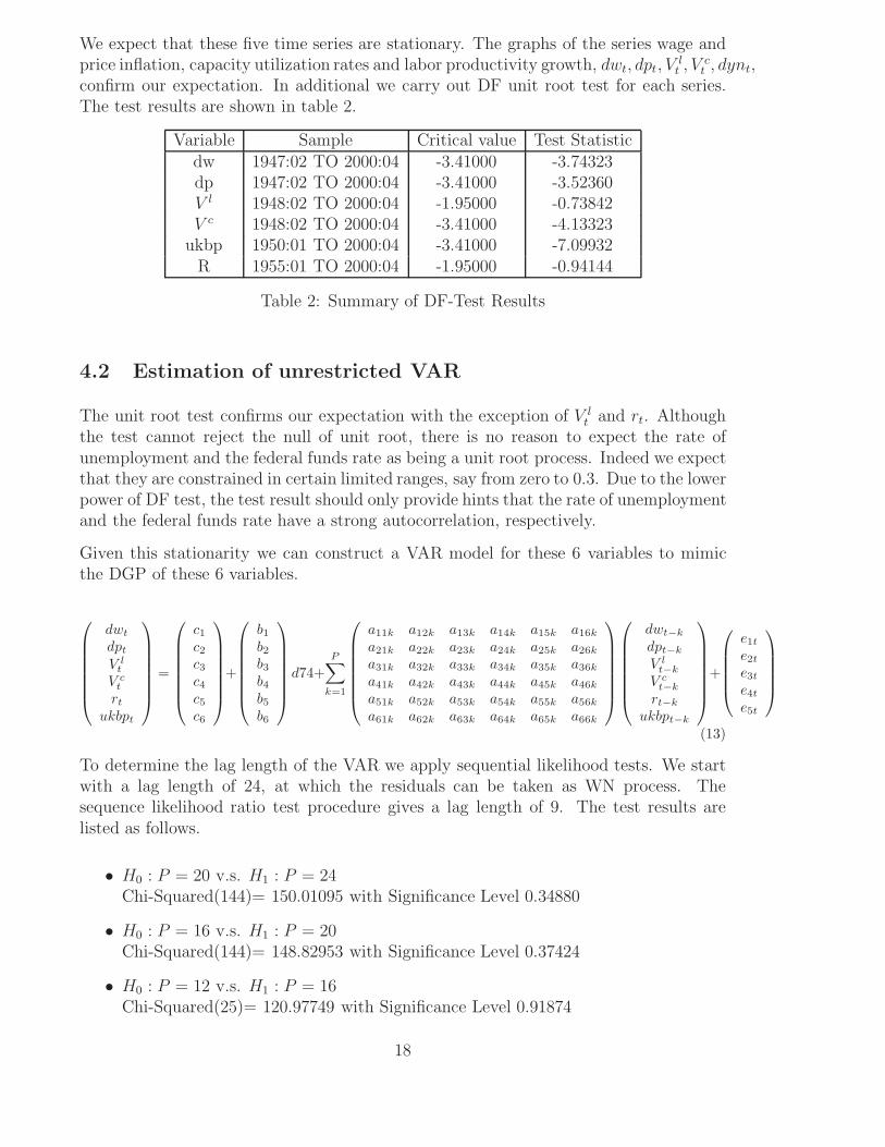
We expect that these five time series are stationary. The graphs of the series wage andprice inflation, capacity utilization rates and labor productivity growth, dwt, dpt, V

lt , V c

t , dynt,confirm our expectation. In additional we carry out DF unit root test for each series.The test results are shown in table 2.

Variable Sample Critical value Test Statisticdw 1947:02 TO 2000:04 -3.41000 -3.74323dp 1947:02 TO 2000:04 -3.41000 -3.52360V l 1948:02 TO 2000:04 -1.95000 -0.73842V c 1948:02 TO 2000:04 -3.41000 -4.13323

ukbp 1950:01 TO 2000:04 -3.41000 -7.09932R 1955:01 TO 2000:04 -1.95000 -0.94144

Table 2: Summary of DF-Test Results

4.2 Estimation of unrestricted VAR

The unit root test confirms our expectation with the exception of V lt and rt. Although

the test cannot reject the null of unit root, there is no reason to expect the rate ofunemployment and the federal funds rate as being a unit root process. Indeed we expectthat they are constrained in certain limited ranges, say from zero to 0.3. Due to the lowerpower of DF test, the test result should only provide hints that the rate of unemploymentand the federal funds rate have a strong autocorrelation, respectively.

Given this stationarity we can construct a VAR model for these 6 variables to mimicthe DGP of these 6 variables.

⎛⎜⎜⎜⎜⎜⎜⎝

dwt

dpt

V lt

V ct

rt

ukbpt

⎞⎟⎟⎟⎟⎟⎟⎠

=

⎛⎜⎜⎜⎜⎜⎜⎝

c1

c2

c3

c4

c5

c6

⎞⎟⎟⎟⎟⎟⎟⎠

+

⎛⎜⎜⎜⎜⎜⎜⎝

b1

b2

b3

b4

b5

b6

⎞⎟⎟⎟⎟⎟⎟⎠

d74+P∑

k=1

⎛⎜⎜⎜⎜⎜⎜⎝

a11k a12k a13k a14k a15k a16k






⎞⎟⎟⎟⎟⎟⎟⎠

⎛⎜⎜⎜⎜⎜⎜⎝

dwt−k

dpt−k

V lt−k

V ct−k

rt−k

ukbpt−k

⎞⎟⎟⎟⎟⎟⎟⎠

+

⎛⎜⎜⎜⎜⎝

e1t

e2t

e3t

e4t

e5t

⎞⎟⎟⎟⎟⎠

(13)

To determine the lag length of the VAR we apply sequential likelihood tests. We startwith a lag length of 24, at which the residuals can be taken as WN process. Thesequence likelihood ratio test procedure gives a lag length of 9. The test results arelisted as follows.

• H0 : P = 20 v.s. H1 : P = 24Chi-Squared(144)= 150.01095 with Significance Level 0.34880



18



According to these test results we use VAR(12) to represent a general model that shouldbe an approximation of the DGP. Because in the dynamic system of (1) – (5) the variableukbpt is treated as exogenous, we factorize the VAR(12) process into a conditional processof dwt, dpt, V

lt , V c

t , rt given ukbpt and the lagged variables, and the marginal process ofukbpt given the lagged variables:

⎛⎜⎜⎜⎜⎝

dwt

dpt

V lt

V ct

rt

⎞⎟⎟⎟⎟⎠ =

⎛⎜⎜⎜⎜⎝

c∗1c∗2c∗3c∗4c∗5

⎞⎟⎟⎟⎟⎠ +

⎛⎜⎜⎜⎜⎝

b∗1b∗2b∗3b∗4b∗5

⎞⎟⎟⎟⎟⎠ d74 +

⎛⎜⎜⎜⎜⎝

a1

a2

a3

a4

a5

⎞⎟⎟⎟⎟⎠ ukpbt (14)

+P∑

k=1

⎛⎜⎜⎜⎜⎝

a∗11k a∗

12k a∗13k a∗

14k a∗15k a∗

16k

a∗21k a∗

22k a∗23k a∗

24k a∗25k a∗

26k

a∗31k a∗

32k a∗33k a∗

34k a∗35k a∗

36k

a∗41k a∗

42k a∗43k a∗

44k a∗45k a∗

46k

a∗51k a∗

52k a∗53k a∗

54k a∗55k a∗

56k

⎞⎟⎟⎟⎟⎠

⎛⎜⎜⎜⎜⎜⎜⎝

dwt−k

dpt−k

V lt−k

V ct−k

rt−k

ukbpt−k

⎞⎟⎟⎟⎟⎟⎟⎠

+

⎛⎜⎜⎜⎜⎝

e∗1t

e∗2t

e∗3t

e∗4t

e∗5t

⎞⎟⎟⎟⎟⎠

ukbpt = c6 +P∑

k=1

(a61k a62k a63k a64k a65k a66k

)

⎛⎜⎜⎜⎜⎜⎜⎝

dwt−k

dpt−k

V lt−k

V ct−k

rt−k

ukbpt−k

⎞⎟⎟⎟⎟⎟⎟⎠

+ e6t (15)

Now we examine if ukbpt can be taken as ”exogenous” variable. The partial system (14) isexactly identified. Hence the variables ut are weakly exogenous for the parameters in thepartial system,7 For the strong exogeneity of ukbpt, we test whether dwt, dpt, V

lt , V c

t , rt

Granger cause ukbpt.

The test is carried out by testing the hypothesis: H0 : aijk = 0, (i = 6; j = 1, 2, 3, 4, 5; k =1, 2, ..., 12) in (15) based on likelihood ratio

• Chi-Squared(60)= 69.157150 with Significance Level 0.19572294

7For detailed discussion see Chen (2003)

19

4.3 Estimation of the Structural Model

As discussed in section 2, the law of motion for real wage rate, eq. (4), can be consideredas the reduced form of two structural equations for dwt and dpt. Assuming that theinflation climate variable is a function of past price inflation rates, the dynamics of thesystem (1) – (5) is equivalently presented by the following equations:

dwt = βw1(Vl − V l)t−1 + κwdpt−1 + (1 − κw)dp12t−1 − βuwukbpt + e1t (16)

dpt = βp1(Vc − V c)t−1 + κpdwt + (1 − κp)dp12t−1 + βupukbpt + e2t (17)

V lt = βV l

1(V c − V c)t−1 − βV l

2(ω − ωo)t−1 + βV l

3(V l − V l)t−1 + e3t (18)

V ct = −αV c(V c− V c)t−1±αω(ω−ωo)−αr((r− p)− (ro− π))+αlV

l +αuukbpt +e4t (19)

rt = −γr(r − ro)t−1 + γp(p − π)t−1 + γV c(V c − V c)t−1 + γω(ω − ωo) + e5t (20)

Obviously the model (16) and (20) is nested in the VAR(12) of (14). Therefore we canuse (14) to evaluate the empirical relevance of the model (16) to (20). First we testwhether the parameter restrictions on (14) implied by (16) to (20) are valid. If the nullof these restrictions cannot be rejected, we will estimate (16) and (20) and then calculatethe empirical estimates for the model (1) to (5).

The structural model (16) to (20) puts 408 restrictions on the unconstrained VAR(12)of system (14). Applying likelihood ratio method we can test the validity of theserestrictions. We get the result:


Obviously, for the period from 1955:1 to 2000:4, the structural model is too restric-tive. However, for the period from 1965:1 to 2000:4 we can not reject the null of theserestrictions. The test result is the following:


Obviously, the specification from (16) to (20) is a valid one for the data set from 1965:1to 2000:4. The estimation results are listed in the appendix. This result shows strongempirical relevance of the law of motions described in (1) – (5) as a model for theeconomy from 1965:1 to 2000:4. It is worthwhile to note that altogether 408 restrictionsare implied through (1) – (5) on the VAR(12) model. A p-value of 0.39 means that (1) –

20

(5) is a much more parsimonious presentation of the DGP than VAR(12), and hencefortha much more efficient model to describe the economic dynamics for this period.

Omitting the insignificant parameters in the structural models and putting the NAIRUstate variables and the like into the constant terms we then get following estimationresult:

dwt = 0.16V lt−1 + 0.29dpt−1 + 0.71dp12t−1 − 0.08ukbpt − 0.15 + e1t (21)

dpt = 0.04V ct−1 + 0.08dwt + 0.92dp12t−1 + 0.01d74t − 0.03 + e2t (22)

V lt = 0.42V c

t−1 − 0.10ukbpt − 0.003d74t + 0.02 + e3t (23)

V ct = −0.08V c

t−1 − 0.08(rt − dpt) + 0.97V l − 0.38ukbpt + 0.08 + e4t (24)

rt = −0.06rt−1 + 0.44dpt−1 + 0.08V ct−1 − 0.06 + e5t (25)

Alternatively we also estimate a slightly modified version of (26) – (30) where we lookat the time rate of change of labor utilization and capacity utilization instead of theirgrowth rate.

dwt = βw1(Vl − V l)t−1 + κwdpt−1 + (1 − κw)dp12t−1 + e1t (26)

dpt = βp1(Vc − V c)t−1 + κpdwt + (1 − κp)dp12t−1 − s · κpdynt−1 (27)

V c = −αV c(V c − V c) ± αω(ω − ωo) − αr((r − p) − (ro − π)) (28)


2(ω − ωo) + βV l

3V c (29)

r = −γr(r − ro) + γp(p − π) + γV c(V c − V c) + γω(ω − ωo) (30)

Omitting the insignificant parameters in the structural models (26) – (30) and puttingall constants of the theoretical model into a single constant term, we get followingestimation result:

dwt = 0.16V lt−1 + 0.26dpt−1 + 0.74dp12t−1 − 0.07ukbpt − 0.15 + e1t (31)

dpt = 0.04V ct−1 + 0.08dwt + 0.92dp12t−1 + 0.01d74t − 0.03 + e2t (32)

V lt = 0.04V c

t−1 − 0.10ukbpt − 0.004d74t + e3t (33)

V ct = −0.12V c

t−1 − 0.12(rt − dpt) − 0.57ukbpt + 0.1 + e4t (34)

rt = −0.08rt−1 + 0.55dpt−1 + 0.06V ct−1 − 0.05 + e5t (35)

Obviously these alternative specifications give similar result as in the formulation ofrestricted VAR(12) we considered beforehand.

21

5 Analyzing the estimated model

In the preceding section we have provided definite answers with respect to the type ofreal wage effect present in the data of the US economy after World War II, concerningthe dependence of aggregate demand on the real wage and the degrees of wage andprice flexibilities. The resulting combination of effects suggest that it is favorable forstability. We stress however that the inflation climate is so far only measured by amoving average of past inflation rates with linearly declining weights. So role of theparameter βπm – which when increased will destabilize the economy – is thus not yetpresent in the considered situation.

We start the stability analysis of the model with estimated parameters in this sectionfrom a basic 3D core situation which we obtain by totally ignoring adjustments in theinflationary climate term by setting πm = π and by interpreting the law of motionfor V l in level terms, i.e., by concentrating on the influence of V c on V l. Integratingthis relationship gives approximately V l = +const (V c)0.42 as can also be confirmed byestimating this level form relationship directly. Under these assumptions, the laws ofmotion (1) – (5) can be reduced to:

V c = const − const V c − const r − const ω (36)

r = −const + const V c − const r + const ω (37)

ω = const + const V c − const ω (38)

We note here that we have inserted here the reduced form expression for the priceinflation rate into the first law of motion for the activity dynamics and rearranged termssuch that the influence of V c and ω appears only once, though both terms appear viatwo channels in this law of motion, one direct channel and one via the price inflationrate. The result of our estimate of this equation is that the latter channel is not changingthe signs of the direct effects of capacity utilization (via the dynamic multiplier) and thereal wage (via consumption and investment behavior).8

A similar treatment applies to the law of motion for the nominal rate of interest, whereprice inflation is again dissolved into its constituent part (in its reduced form expression)and where again the influence of V l in this expression is replaced by V c through Okun’sLaw. Again the direct effect of ω in the Taylor rule is assumed to dominate the indirecton (via the inflation rate), as this was confirmed by our empirical estimate of this lawof motion.9

Finally, the law of motion for real wages themselves is obtained from the two estimatedstructural laws of motion for wage and price inflation in the way shown in section 2. Wehave a positive influence of capacity utilization on the growth rate of real wages, sincethe wage Phillips curve dominates the outcome here and a negative influence of realwages on their rate of growth due to the signs of the Blanchard / Katz error correctionterms in the wage and the price dynamics.10

8to be estimated in this form: sign of βp2 − κpβw2 does not matter?9to be estimated in this form: sign of βp2 − κpβw2 does not matter?

10to be estimated in this form: DFP to be suppressed?

22

On this basis we arrive at the following sign structure for the Jacobian of the 3D dynamicsat the interior steady state of the above reduced model:

J =

⎛⎝ − − −

+ − ++ 0 −

⎞⎠ .

We therefrom immediately get that the trace of this matrix is negative, the sum a2 ofprincipal minors of order two is positive and a determinant of the whole matrix that isnegative. The coefficients ai, i = 1, 2, 3 of the Routh Hurwitz polynomial of this matrixare therefore all positive as demanded by the Routh Hurwitz stability conditions. Theremaining stability condition is

a1a2 − a3 = (−traceJ)a2 − detJ > 0.

With respect to this condition we first of all see that the determinant of J is given by:

J33(J11J22 − J12J21) + J31(J12J23 − J13J22).

With respect to this expression we see that the first term is dominated by (−traceJ)a2

and can thus be canceled from the calculation of a1a2 − a3. The same holds true for theterm −J31J13J22) in the determinant of J, while the remaining, non-neutralized termJ31J12J23 in this determinant can be made arbitrary small if the dependence of theinterest rate policy rule on the unconventional influence of the real wage on this interestrate setting is made sufficiently small. the may however exist a variety of other situationswhere the above sign structure of the Jacobian of the considered 3D dynamics will lead toasymptotic stability, in particular if the actual size of the estimated parameters is takeninto account in addition. The real wage effect that is now included into the dynamicsof the private sector therefore seems to create not much harm for the stability of thesteady state of the considered dynamics, in particular due to its negative influence onthe rate of change of economic activity.

Increasing price flexibility may however change this situation, since growth rate of eco-nomic activity can thereby be made to depend positively on the level of economic activity,leading to an unstable dynamic multiplier process in the trace of J under such circum-stances. Furthermore, such increasing price flexibility will also give rise to a negativedependence of the real wage on economic activity and thus lead to further sign changesin the Jacobian J. A further destabilizing mechanism is introduced if we add again thelaw of motion for the inflationary climate surrounding the current evolution of priceinflation.

Under this latter extension to a 4D dynamical system the Jacobian J is augmented inits sign structure in the following way:

J =

⎛⎜⎜⎝

− − − ++ − + ++ 0 − 0+ 0 ± 0

⎞⎟⎟⎠ .

As the positive entries J14, J41 show there is now a destabilizing feedback chain, lead-ing from increases in economic activity to increases in inflation and expected inflation

23

and from there back to increases in economic activity, through the real rate of interestchannel. This destabilizing so-called Mundell effect must become dominant as the ad-justment speed of the climate expression βπm is increased. The Blanchard / Katz errorcorrection terms in the fourth row of J , obtained from the reduced form price Phillipscurve, that are (as only further terms) associated with the speed parameter βπm , are ofno help here, since they do not appear in combination with the parameter βπm in thesum of principal minors of order 2. In this sum the parameter βπm thus only enters onceand with a negative sign implying that this sum can be made negative if this parameteris chosen sufficiently large.

Furthermore, making use of the reduced form expression for the term p−πm one can eas-ily show – under one mild assumption – that the sign structure in the above 4D Jacobiancan be reduced to the following form without change in the sign of the correspondingJacobians:

J =

⎛⎜⎜⎝

0 − 0 00 0 0 +0 0 − 0+ 0 0 0

⎞⎟⎟⎠ .

This follows, since we can reduce the first two laws of motion to the use of πm inthe place of p and since the last two laws can be reduced to βw and βp terms solely,respectively, which in turns implies a further reduction to a negative influence of only ωon its rate of growth and a positive sole influence of V c on πm, everything without changeof sign in the considered determinants. Assuming then that interest rate smoothing issufficiently weak allows for the conclusion that the 4D determinant exhibits a positivesign throughout.

We therefrom in sum get that the 4D dynamics will be convergent for small speedsof adjustments βπm, while it will be divergent for parameters βπm chosen sufficientlylarge. The Mundell effect thus works as expected from a partial perspective. There willbe a unique Hopf bifurcation point βH

πm in between where the system loses asymptoticstability in a cyclical fashion by the death of an unstable or the birth of a stable limitcycle. Yet sooner or later purely explosive behavior will be established, where thereis no room any more for persistent economic fluctuations in the real and the nominalmagnitudes.

Remark: The Livingston index for consumer price index inflation may be used to measurethe size of the parameter βπm on the basis of this measure for an inflationary climate.Comparison with DFP?

Modifying the above model finally in order to incorporate into it a simple dynamicversion of Okun’s law, see (2), gives rise to its following respecification:

V c = const − αV cV c − αωω − αr(r − p) (39)

V l = const + βV l1V c + βV l

2V c (40)

r = const − γrr + γpp + γV cV c + γωω (41)

ω = const + κ[(1 − κp)(βw1Vl − βw2ω) − (1 − κw)(βp1V

c + βp2ω)] (42)

πm = βπm(p − πm) (43)

24

withp = const + κ[βp1V

c + βp2ω + κp(βw1Vl − βw2ω)] + πm

with the variables: capacity utilization V c, the rate of employment V l, the rate of interestr, and the inflationary climate πm, and the real wage ω.

Inserting finally the estimated values into these reformulated equations gives rise to thefollowing numerical specification of this model type

V c = const − 0.08V c − 0.38ω − 0.089(r − p)

V l = const + 0.01V c + 0.15V c

r = const − 0.08r + 0.44p + 0.08V c

ω = const + 0.10V l − 0.025V c − 0.067ω

πm = βπm(p − πm), βπm to be determined still

withp = const + 0.04V c + 0.13V l + 0.01ω + πm,

based on the estimates βw1 = 0.16, βw2 = −0.08, βp1 = 0.04, βp2 = 0, κw = 0.29, andκp = 0.08 (κ = 1.08).

We clearly see again in these equations the stabilizing role of the dynamic multiplier,the dominance of investment demand in the determination of real wage influences onaggregate demand and the multiplier, as well as the negative real rate of interest effecton changes in goods markets’ activity levels.

In the law of motion describing the evolution of the real wage, we have the expectedpositive influence of the rate of employment and the negative influence of the rate ofcapacity utilization (that drives the price rate of inflation), as well as the joint workingof the Blanchard and Katz (2000) error correction mechanisms, but only in the wagedynamics. We know from the estimates of the dw, dp equations that their difference mustcontain 0.326dyn as resulting influence of labor productivity growth, but do neglect thishere, since unit wage costs have been detrended by the bandpass filter in the estimationof the wage and price Phillips curves.

6 Conclusions and outlook

We have considered in this paper an significant extension and modification of the tradi-tional approach to AS-AD growth dynamics that allows us to avoid dynamical inconsis-tencies of the traditional Neoclassical synthesis, stage I, and also to overcome empiricalweaknesses of the New Keynesian approach, the Neoclassical synthesis, stage II, thatarise from the assumption of purely forward looking behavior. Conventional wisdomavoids the stability problems then generated in these model types by just assumingglobal asymptotic stability through the adoption of non-predetermined variables andthe application of the so-called jump-variable technique.

This approach of the Rational Expectations School is however much more than justthe consideration of rational expectations, but in fact the assumption of hyperperfect

25

foresight coupled with a solution method that avoids all potential instabilities of macro-dynamic economic systems by assumption. In the present context, this approach wouldimpose the condition that prices – and also nominal wages – must be allowed to jumpin a particular way in order to establish by assumption the stability of the investigateddynamics.

By contrast, our alternative approach – which allows for sluggish wage as well as priceadjustment and also for certain economic climate variables, representing the medium-run evolution of inflation (and in Asada, Chen, Chiarella and Flaschel (2004) also excessprofitability) – completely bypasses such stability assumptions. Instead it allows todemonstrate in a detailed way, guided by the intuition behind important macroeconomicfeedback channels, local asymptotic stability under certain plausible assumptions (indeedvery plausible from the perspective of a Keynesian feedback channel theory), cyclicalloss of stability when these assumptions are violated (if speeds of adjustment becomesufficiently high), and even explosive fluctuations in the case of further increases of thecrucial speeds of adjustment of the model. In the latter case extrinsic nonlinearities haveto be introduced in order to tame the explosive dynamics as in some of the examplesin Chiarella and Flaschel (2000, Ch.6,7) where a kinked Phillips curve is employed toachieve global boundedness.

The stability features of this – in our view properly reformulated – Keynesian dynamicsare based on specific interactions of traditional Keynes- and Mundell-effects or real rateof interest effects (here present only in the employed investment function) with so-calledRose or real-wage effects, see Chiarella and Flaschel (2000) for their introduction, whichin the present framework simply means that increasing wage flexibility is stabilizingand increasing price flexibility destabilizing, based on the fact that aggregate demandhere depends negatively on the real wage (due to the assumed investment function) anddue to the extended types of Phillips curves we have employed in our new approachto traditional Keynesian growth dynamics. The interaction of these three effects iswhat explains the obtained stability results under the in this case not very importantassumption of myopic perfect foresight, on wage as well as price inflation, and thus givesrise to a traditional type of Keynesian business cycle theory, not at all plagued by theanomalies of the textbook AS-AD dynamics, see Chiarella, Flaschel and Franke (2004)for a detailed treatment and critique of this textbook approach.

The model of this paper will be numerically explored in a companion paper, Asada,Chiarella, Flaschel and Hung (2004), in order to analyze in greater depth, and also withthe empirical background here generated, the interaction of the various feedback channelspresent in the considered dynamics. At that point we will make use of LM curves aswell as Taylor interest rate policy rules, kinked Phillips curves and Blanchard / Katzerror correction mechanisms in order to investigate in detail the various ways by whicha locally unstable dynamics can be made bounded and thus viable. The question then iswhich behavioral assumption on private behavior and fiscal and monetary policy – onceviability is achieved – can reduce the volatility of the resulting persistent fluctuations.

Our work on related models suggests that the interest rate policy rule may not besufficient to tame the explosive dynamics in all conceivable cases, or even make it con-vergent. But when viability is achieved – for example by downward wage rigidity –

26

we can investigate the parameter corridor where monetary policy for example can re-duce the endogenously generated fluctuations of this approach to Keynesian businessfluctuations.

Taking all this together our general conclusion will be that this framework not onlyovercomes the anomalies of the Neoclassical Synthesis, Stage I, but also provides a co-herent alternative to the New Keynesian theory of the business cycle, as sketched in Gali(2000). This alternative is based on disequilibrium in the market for goods and labor,on sluggish adjustment of prices as well as wages and on myopic perfect foresight inter-acting with certain economic climate expression with a rich array of dynamic outcomesthat provide great potential for further generalizations. Some of these generalizationsare considered in Chiarella, Flaschel, Groh and Semmler (2000) and Chiarella, Flascheland Franke (2004). Our overall approach, which may be called a disequilibrium ap-proach to business cycle modelling, thus provides a theoretical framework within whichto consider the contributions of authors such as Zarnowitz (1999) who also stresses thedynamic interaction of many traditional macroeconomic building blocks.

References

Asada, T., Chiarella, C., Flaschel, P. and R. Franke (2003): Open EconomyMacrodynamics. An Integrated Disequilibrium Approach. Heidelberg: SpringerVerlag.

Asada, T., Chen, P., Chiarella, C. and P. Flaschel (2004): Keynesian dynam-ics and the wage-price spiral. A baseline disequilibrium approach. UTS Sydney:School of Finance and Economics.

Asada, T., Chiarella, C., Flaschel, P. and H. Hung (2004): Keynesian dy-namics and the wage-price spiral. Numerical Analysis of a Baseline DisequilibriumModel. UTS Sydney: School of Finance and Economics.

Barro, X. (1994): The aggregate supply / aggregate demand model. Eastern EconomicJournal, 20, 1 – 6.

Blanchard, O.J. and L. Katz (2000): Wage dynamics: Reconciling theory andevidence. American Economic Review. Papers and Proceedings, 69 – 74.

Chen Pu (2003): Weak Exogeneity in Simultaneous Equations System. University ofBielefeld: Discussion Paper No. 502.

Chen, P. and Flaschel, P. (2004): Testing the dynamics of wages and prices for theUS economy. Bielefeld: Center for Empirical Macroeconomics. Working paper.

Chiarella, C. and P. Flaschel (2000): The Dynamics of Keynesian MonetaryGrowth: Macro Foundations. Cambridge, UK: Cambridge University Press.

Chiarella, C., P. Flaschel, G. Groh and W. Semmler (2000): Disequilibrium,Growth and Labor Market Dynamics. Heidelberg: Springer Verlag.

27

Chiarella, C., Flaschel, P. and R. Franke (2004): .A Modern Approach to Key-nesian Business Cycle Theory. Qualitative Analysis and Quantitative Assessment.Cambridge, UK: Cambridge University Press, to appear.

Flaschel, P. and H.-M.Krolzig (2004): Wage and price Phillips curves. An em-pirical analysis of destabilizing wage-price spirals. Oxford: Oxford University.Discussion paper.

Flaschel, P., Kauermann, G. and W. Semmler (2004): Testing wage and pricePhillips curves for the United States. Bielefeld University: Center for EmpiricalMacroeconomics, Discussion Paper.

Gali, J. (2000): The return of the Phillips curve and other recent developments inbusiness cycle theory. Spanish Economic Review, 2, 1 – 10.

Gali, J., Gertler, M. and J.D. Lopez-Salido (2003): Robustness of the Es-timates of the Hybrid New Keynesian Phillips Curve. Paper presented at theCEPR Conference: The Phillips curve revisited. Berlin: June 2003

Groth, C. (1992): Some unfamiliar dynamics of a familiar macromodel. Journal ofEconomics, 58, 293 – 305.

Eller, J.W. and R.J. Gordon (2003): Nesting the New Keynesian Phillips Curvewithin the Mainstream Model of U.S. Inflation Dynamics. Paper presented at theCEPR Conference: The Phillips curve revisited. Berlin: June 2003

Mankiw, G. (2001): The inexorable and mysterious tradeoff between inflation andunemployment. Economic Journal, 111, 45 – 61.

Rose, H. (1967): On the non-linear theory of the employment cycle. Review of Eco-nomic Studies, 34, 153 – 173.

Rudebusch, G.D. and L.E.O. Svensson (1999): Policy rules for inflation targeting.In: J.B.Talor (ed.): Monetary Policy Rules. Chicago: Chicago University Press.

Sargent, T. (1987): Macroeconomic Theory. New York: Academic Press.

Tobin, J. (1975): Keynesian models of recession and depression. American EconomicReview, 65, 195 – 202.

Woodford, M. (2003): Interest and Prices. Princeton: Princeton University Press.

Zarnowitz, V. (1999): Theory and History Behind Business Cycles: Are the 1990sthe onset of a Golden Age? NBER Working paper 7010,http://www.nber.org/papers/w7010.

28

7 Appendix: Estimation Results

Single Equation Estimation of (21) to (25)

Linear Regression - Estimation by Least SquaresDependent Variable DWQuarterly Data From 1965:01 To 2000:04Usable Observations 143 Degrees of Freedom 138Total Observations 144 Skipped/Missing 1

Centered R**2 0.624227 R Bar **2 0.613335Uncentered R**2 0.932527 T x R**2 133.351Mean of Dependent Variable 0.0144268217Std Error of Dependent Variable 0.0067728907Standard Error of Estimate 0.0042115453Sum of Squared Residuals 0.0024477217Regression F(4,138) 57.3108Significance Level of F 0.00000000Durbin-Watson Statistic 1.623078

Variable Coeff Std Error T-Stat Signif*******************************************************************************1. DP{1} 0.197140530 0.148555607 1.32705 0.186684052. DFP 0.929962056 0.189391042 4.91027 0.000002533. VL{1} 0.195780837 0.032693348 5.98840 0.000000024. UKBP{1} -0.068700307 0.034212646 -2.00804 0.046591125. Constant -0.181534056 0.031220303 -5.81462 0.00000004

Linear Regression - Estimation by Least SquaresDependent Variable DPQuarterly Data From 1965:01 To 2000:04Usable Observations 144 Degrees of Freedom 139Centered R**2 0.835171 R Bar **2 0.830428Uncentered R**2 0.959113 T x R**2 138.112Mean of Dependent Variable 0.0105799813Std Error of Dependent Variable 0.0060979256Standard Error of Estimate 0.0025110731Sum of Squared Residuals 0.0008764628Regression F(4,139) 176.0747Significance Level of F 0.00000000Durbin-Watson Statistic 1.599777

Variable Coeff Std Error T-Stat Signif*******************************************************************************1. DW{1} 0.087894111 0.046473210 1.89129 0.060666932. DFP 0.935253173 0.061707858 15.15614 0.000000003. VC{1} 0.046153826 0.005654010 8.16303 0.000000004. D74 0.009987686 0.001840223 5.42743 0.00000025

29

5. Constant -0.038381571 0.004726692 -8.12018 0.00000000

Linear Regression - Estimation by Least SquaresDependent Variable DVLQuarterly Data From 1965:01 To 2000:04Usable Observations 142 Degrees of Freedom 136Total Observations 144 Skipped/Missing 2

Centered R**2 0.529833 R Bar **2 0.512547Uncentered R**2 0.530008 T x R**2 75.261Mean of Dependent Variable 0.0000688254Std Error of Dependent Variable 0.0035759981Standard Error of Estimate 0.0024966844Sum of Squared Residuals 0.0008477469Regression F(5,136) 30.6517Significance Level of F 0.00000000Durbin-Watson Statistic 2.056523

Variable Coeff Std Error T-Stat Signif*******************************************************************************1. VL{1} 0.505469389 0.085304889 5.92544 0.000000022. VL{2} -0.520280734 0.078411280 -6.63528 0.000000003. VC{1} -0.007799417 0.009128566 -0.85440 0.394387764. UKBP -0.109893359 0.024329306 -4.51691 0.000013485. D74 -0.003587478 0.001851895 -1.93719 0.054794806. Constant 0.020331826 0.017135470 1.18653 0.23747990

Linear Regression - Estimation by Least SquaresDependent Variable DVCQuarterly Data From 1965:01 To 2000:04Usable Observations 142 Degrees of Freedom 137Total Observations 144 Skipped/Missing 2

Centered R**2 0.481545 R Bar **2 0.466407Uncentered R**2 0.481817 T x R**2 68.418Mean of Dependent Variable -0.000323944Std Error of Dependent Variable 0.014185973Standard Error of Estimate 0.010362488Sum of Squared Residuals 0.0147112173Regression F(4,137) 31.8116Significance Level of F 0.00000000Durbin-Watson Statistic 1.638300

Variable Coeff Std Error T-Stat Signif*******************************************************************************1. VC{1} -0.124199856 0.021085861 -5.89020 0.000000032. DVL{1} 1.335384864 0.298778877 4.46948 0.000016293. RRATE{1} -0.157024873 0.034250470 -4.58460 0.000010154. UKBP -0.389488266 0.101354961 -3.84281 0.000185395. Constant 0.110333381 0.017685736 6.23855 0.00000001

30

Linear Regression - Estimation by Least SquaresDependent Variable DRATEQuarterly Data From 1965:01 To 2000:04Usable Observations 144 Degrees of Freedom 140Centered R**2 0.107048 R Bar **2 0.087914Uncentered R**2 0.107363 T x R**2 15.460Mean of Dependent Variable 0.0002011574Std Error of Dependent Variable 0.0107603680Standard Error of Estimate 0.0102764963Sum of Squared Residuals 0.0147848928Regression F(3,140) 5.5945Significance Level of F 0.00118480Durbin-Watson Statistic 1.689986

Variable Coeff Std Error T-Stat Signif*******************************************************************************1. DFP 0.425074027 0.218103715 1.94895 0.053300452. VC{1} 0.067787859 0.021178390 3.20080 0.001695943. RATE{1} -0.097427370 0.036990822 -2.63383 0.009392624. Constant -0.052760785 0.018009545 -2.92960 0.00396402

3SLS System Estimation of () to ()

Linear Systems - Estimation by Seemingly Unrelated Regressions

Iterations Taken 2Quarterly Data From 1965:01 To 2000:04Usable Observations 142Total Observations 144 Skipped/Missing 2

Dependent Variable DWCentered R**2 0.628606 R Bar **2 0.465648Uncentered R**2 0.932844 T x R**2 132.464Mean of Dependent Variable 0.0144055704Std Error of Dependent Variable 0.0067920795Standard Error of Estimate 0.0049649699Sum of Squared Residuals 0.0024157908Durbin-Watson Statistic 1.652995


31

Dependent Variable DPCentered R**2 0.832898 R Bar **2 0.759578Uncentered R**2 0.959052 T x R**2 136.185Mean of Dependent Variable 0.0106653293Std Error of Dependent Variable 0.0060978384Standard Error of Estimate 0.0029899457Sum of Squared Residuals 0.0008760980Durbin-Watson Statistic 1.605294

Variable Coeff Std Error T-Stat Signif*******************************************************************************6. DW{1} 0.082390164 0.045812523 1.79842 0.072110457. DFP 0.942049199 0.061753718 15.25494 0.000000008. VC{1} 0.046450989 0.005597851 8.29800 0.000000009. D74 0.010522748 0.001763341 5.96751 0.0000000010. Constant -0.038614621 0.004684016 -8.24391 0.00000000

Dependent Variable DVLCentered R**2 0.522405 R Bar **2 0.305765Uncentered R**2 0.522583 T x R**2 74.207Mean of Dependent Variable 0.0000688254Std Error of Dependent Variable 0.0035759981Standard Error of Estimate 0.0029795500Sum of Squared Residuals 0.0008611387Durbin-Watson Statistic 1.899020

Variable Coeff Std Error T-Stat Signif*******************************************************************************11. VL{1} 0.442497469 0.075962496 5.82521 0.0000000112. VL{2} -0.453181272 0.071466282 -6.34119 0.0000000013. VC{1} -0.007408317 0.007570160 -0.97862 0.3277673614. UKBP -0.102245939 0.022041647 -4.63876 0.0000035115. D74 -0.002718577 0.001376292 -1.97529 0.0482350916. Constant 0.016128849 0.013268927 1.21554 0.22416201

Dependent Variable DVCCentered R**2 0.453939 R Bar **2 0.214341Uncentered R**2 0.454225 T x R**2 64.500Mean of Dependent Variable -0.000323944Std Error of Dependent Variable 0.014185973Standard Error of Estimate 0.012574082Sum of Squared Residuals 0.0154945396Durbin-Watson Statistic 1.538509

Variable Coeff Std Error T-Stat Signif*******************************************************************************

32

17. VC{1} -0.107396969 0.020385633 -5.26827 0.0000001418. DVL{1} 0.990268556 0.260254619 3.80500 0.0001418019. RRATE{1} -0.087342645 0.025881467 -3.37472 0.0007389120. UKBP -0.389421984 0.087005531 -4.47583 0.0000076121. Constant 0.092439937 0.016944697 5.45539 0.00000005

Dependent Variable DRATECentered R**2 0.098748 R Bar **2 -0.283601Uncentered R**2 0.099027 T x R**2 14.062Mean of Dependent Variable 0.0001899061Std Error of Dependent Variable 0.0108345824Standard Error of Estimate 0.0122751627Sum of Squared Residuals 0.0149172824Durbin-Watson Statistic 1.735485

Variable Coeff Std Error T-Stat Signif*******************************************************************************22. DFP 0.425510274 0.194647582 2.18605 0.0288116023. VC{1} 0.071522021 0.020739654 3.44856 0.0005635824. RATE{1} -0.063107081 0.033596640 -1.87837 0.0603299125. Constant -0.058282751 0.017563513 -3.31840 0.00090535

Likelihood Ratio Test of the Structural Restrictions

Chi-Squared(408)= 414.104639 with Significance Level 0.39322678

Chi-Squared(3)= 3.929183 with Significance Level 0.26921333

3SLS - System Estimation under Restrictions

Linear Model - Estimation by Restricted RegressionDependent Variable UKBP

Variable Coeff*****************************************1. DP{1} 0.2852968562. DFP 0.7147031443. VL{1} 0.1597039124. UKBP{1} -0.0782372425. Constant -0.1463292896. DW{1} 0.0813928277. DFP 0.9186071738. VC{1} 0.0453276739. D74 0.01070880210. Constant -0.037436331

33

11. VL{1} 0.46179946712. VL{2} -0.46179946713. VC{1} -0.01085497414. UKBP -0.10363031415. D74 -0.00266560116. Constant 0.00890258917. VC{1} -0.10816656818. DVL{1} 1.00298766119. RRATE{1} -0.09139643220. UKBP -0.38627053521. Constant 0.09331277622. DFP 0.43859549923. VC{1} 0.07194054824. RATE{1} -0.064939038

3SLS Estimation of the System (31) to (35)

Linear Systems - Estimation by Seemingly Unrelated Regressions

Iterations Taken 2Quarterly Data From 1965:01 To 2000:04Usable Observations 140Total Observations 144 Skipped/Missing 4

Dependent Variable DWCentered R**2 0.622469 R Bar **2 0.469931Uncentered R**2 0.933152 T x R**2 130.641Mean of Dependent Variable 0.0145273297Std Error of Dependent Variable 0.0067628354Standard Error of Estimate 0.0049237398Sum of Squared Residuals 0.0024000782Durbin-Watson Statistic 1.647187


Dependent Variable DPCentered R**2 0.831840 R Bar **2 0.763897Uncentered R**2 0.959287 T x R**2 134.300Mean of Dependent Variable 0.0107511047Std Error of Dependent Variable 0.0060983439

34

Standard Error of Estimate 0.0029632119Sum of Squared Residuals 0.0008692818Durbin-Watson Statistic 1.611661

Variable Coeff Std Error T-Stat Signif*******************************************************************************6. DW{1} 0.084652477 0.046020765 1.83944 0.065850377. DFP 0.945391907 0.061584060 15.35124 0.000000008. VC{1} 0.048304943 0.005649662 8.55006 0.000000009. D74 0.010211416 0.001762877 5.79247 0.0000000110. Constant -0.040181448 0.004711322 -8.52870 0.00000000

Dependent Variable DLVLCentered R**2 0.373032 R Bar **2 0.137144Uncentered R**2 0.373142 T x R**2 52.240Mean of Dependent Variable 0.0000472956Std Error of Dependent Variable 0.0035954978Standard Error of Estimate 0.0033398603Sum of Squared Residuals 0.0011266214Durbin-Watson Statistic 1.432012

Variable Coeff Std Error T-Stat Signif*******************************************************************************11. DLVC{1} 0.046349029 0.011887032 3.89913 0.0000965412. UKBP{1} -0.103750948 0.023763966 -4.36589 0.0000126613. D74 -0.003998848 0.001592853 -2.51049 0.01205625

Dependent Variable DLVCCentered R**2 0.291811 R Bar **2 0.015617Uncentered R**2 0.292685 T x R**2 40.976Mean of Dependent Variable -0.000625869Std Error of Dependent Variable 0.017872618Standard Error of Estimate 0.017732507Sum of Squared Residuals 0.0314441821Durbin-Watson Statistic 1.377719

Variable Coeff Std Error T-Stat Signif*******************************************************************************14. VC{1} -0.118574486 0.023993282 -4.94199 0.0000007715. RRATE{1} -0.125010402 0.036489460 -3.42593 0.0006126916. UKBP{1} -0.578025142 0.113297116 -5.10185 0.0000003417. Constant 0.103163866 0.019990019 5.16077 0.00000025

Dependent Variable DRATECentered R**2 0.214185 R Bar **2 -0.103316Uncentered R**2 0.214349 T x R**2 30.009Mean of Dependent Variable 0.0001569048

35

Std Error of Dependent Variable 0.0109072628Standard Error of Estimate 0.0114568646Sum of Squared Residuals 0.0129947148Durbin-Watson Statistic 1.885672

Variable Coeff Std Error T-Stat Signif*******************************************************************************18. DP{1} 0.560533027 0.163625222 3.42571 0.0006131919. VC{1} 0.062208851 0.017968086 3.46219 0.0005358120. RATE{1} -0.081392279 0.031553949 -2.57946 0.0098953721. Constant -0.050592198 0.015051926 -3.36118 0.0007761122. D74{1} -0.022586355 0.006685026 -3.37865 0.00072843

Chi-Squared(404)= 450.332794 with Significance Level 0.05538152Chi-Squared(2)= 3.229649 with Significance Level 0.19892557

Linear Model - Estimation by Restricted RegressionDependent Variable UKBP

Variable Coeff*****************************************1. DP{1} 0.2626186842. DFP 0.7373813163. VL{1} 0.1649853424. UKBP{1} -0.0702520585. Constant -0.1512470526. DW{1} 0.0836964337. DFP 0.9163035678. VC{1} 0.0469577979. D74 0.01044395810. Constant -0.03875986611. DLVC{1} 0.04662183212. UKBP{1} -0.10360369413. D74 -0.00401623514. VC{1} -0.11875957915. RRATE{1} -0.12651534516. UKBP{1} -0.57862296317. Constant 0.10340422218. DP{1} 0.55905450619. VC{1} 0.06226845320. RATE{1} -0.08167719621. Constant -0.05060487422. D74{1} -0.022604143

36

Documents

Keynesian Dynamics and the Wage-Price Spiral. Estimating a