Embed Size (px)
Citation preview
arX
iv:1
412.
7523
v2 [
mat
h-ph
] 1
2 M
ay 2
015
Classical Noether’s theory with application to the
linearly damped particle
Raphael Leone and Thierry Gourieux
Universite de Lorraine, IJL, Groupe de Physique Statistique (UMR CNRS 7198)
F-54506 Vandœuvre-les-Nancy cedex, France
E-mail: [email protected]
Abstract. This paper provides a modern presentation of Noether’s theory in the
realm of classical dynamics, with application to the problem of a particle submitted
to both a potential and a linear dissipation. After a review of the close relationships
between Noether symmetries and first integrals, we investigate the variational point
symmetries of the Lagrangian introduced by Bateman, Caldirola and Kanai. This
analysis leads to the determination of all the time-independent potentials allowing
such symmetries, in the one-dimensional and the radial cases. Then we develop a
symmetry-based transformation of Lagrangians into autonomous others, and apply it
to our problem. To be complete, we enlarge the study to Lie point symmetries which
we associate logically to Noether ones. Finally, we succinctly address the issue of a
‘weakened’ Noether’s theory, in connection with ‘on-flows’ symmetries and non-local
constant of motions, for it has a direct physical interpretation in our specific problem.
Since the Lagrangian we use gives rise to simple calculations, we hope that this work
will be of didactic interest to graduate students, and give teaching material as well as
food for thought for physicists regarding Noether’s theory and the recent developments
around the idea of symmetry in classical mechanics.
PACS numbers: 02.30.Hq,45.20.Jj,45.50.Dd
Keywords: Classical mechanics, Noether symmetries, Lie symmetries, first integrals,
non-conservative systems, Bateman-Caldirola-Kanai Lagrangian
Classical Noether’s theory with application to the linearly damped particle 2
1. Introduction
In Lagrangian mechanics, a primary method for taking into account non-conservative
forces is to add their generalized counterparts in the Euler-Lagrange equations [1, 2].
But by doing so, one loses the variational framework on which the ‘wonderful’ [3]
Noether’s theory [4, 5] relies naturally. Then, if we are interested in the study of
conservation laws, one might use alternative techniques, focused on the equations of
motion. Among the most elegant are Lie’s theory [6–8] and λ-symmetries [9, 10], Jacobi
last multipliers [1, 11–13], or methods based upon integrating factors [14–16]. They are
highly interconnected [17–20] and each of them stands more or less on some symmetry
concept. A second, albeit related, approach consists in trying to find a ‘non-standard’
Lagrangian encoding all the dynamics so as to recover a genuine variational framework
on which Noether’s theory can be applied. That demands to obtain a solution to the
inverse Lagrange problem, as first posed by Helmholtz in 1887 [1, 21, 22], e.g. by seeking
a Jacobi last multiplier [23]. However, solutions may be not tractable, or none may exist,
or even the resulting Lagrangians may be very cumbersome. A last possibility is to
extend Noether’s theory to the primary formulation [24], or at the level of d’Alembert’s
principle [25].
Fortunately, after the seminal works of Bateman [26], Caldirola [27], and Kanai [28]
(BCK), the problem of a particle submitted to both a potential V and a linear drag
force f = −2mγv, where m is the particle’s mass and γ the dissipation rate, is known
to admit the quite simple Lagrangian
LBCK(r, v, t) =
(1
2mv2 − V
)e2γt. (1)
Indeed, the corresponding Euler-Lagrange equations are, in vector notation,
E(LBCK) =
(m
dv
dt+∂V
∂r+ 2mγv
)e2γt = 0.
Since the weight factor e2γt does never vanish during time, the above equations give a
faithful account of the dynamics‡. This Lagrangian has interesting properties: (i) it
is close in form and tends to the standard conservative Lagrangian T − V when the
dissipation rate γ goes to zero; (ii) it is universally valid for all potentials. Those are
among the reasons why, for decades, the BCK Lagrangian has attracted attention [29–
35] and why it has become a kind of paragon for the thorny question of canonical
quantization of non-conservative systems [28, 36–39], first and foremost addressed within
the ubiquitous harmonic oscillator. In this article, however, we will not enter this
epistemological debate. We will remain at the classical standpoint: our purpose here is
to analyse the variational symmetries of LBCK and the conservation laws they induce.
The paper is organized as follows. We give in section 2 an overview of Noether’s
theorem in classical mechanics and highlight the intimate connections between Noether
‡ The BCK Lagrangian can be adapted to a time-dependent dissipation rate; it suffices to replace γt
by∫γ(t) dt in the exponential factor of (1).
Classical Noether’s theory with application to the linearly damped particle 3
symmetries and first integrals. Then, we begin section 3 by seeking Noether point
symmetries (NPS) of the one-dimensional BCK Lagrangian. It brings us to all the
time-independent potentials admitting at least one NPS. They are divisible into four
classes, including the very special family of at most quadratic polynomials which are
known to possess the maximal number of independent NPS: 5 [40]. As a second step,
we make an excursion into the central problems in three dimensions. On the one hand,
rotational symmetry about the center of force emerges naturally, but, on the other
hand, we show that the angular momentum breaks some of the symmetries previously
identified in the unidimensional case.
Section 4 is devoted to symmetry-based transformations of Lagrangians into
autonomous others. By construction, the latter lead to Hamiltonians which coincide
with the first integrals generated by the symmetries. More precisely, we develop a
systematic scheme for carrying out such a mapping from the existence of a NPS, and
apply it to the BCK Lagrangian. In section 5, we enlarge the study to Lie point
symmetries (LPS) of the Euler-Lagrange equations. We show that the time translation
invariance is the only additional point symmetry, with the notable exception of potentials
at most quadratic. Indeed, they reach a LPS algebra of maximal dimension: 8 [40]. It
is en passant the opportunity to give the eight first integrals associated to a basis of
those algebra for the linear potential, which we did not find in the literature. Then,
thanks to the converse of Noether’s theorem, we associate to each of these additional
symmetries a Noether one. Finally, we discuss in section 6 a weak version of Noether’s
theorem, in terms of which any first integral amounts to a local expression of the BCK
action functional along the solution curves.
2. Noether’s theorem in classical mechanics
2.1. The general statement of Noether’s theorem; Killing-type equations
Let us consider a dynamical system governed by a regular Lagrangian L in terms of
n generalized coordinates qi. Hamilton’s variational principle applied to the action
functional
A :=
∫L(q, q, t) dt
yields a set of n second-order differential equations Ei(L) = 0, where
Ei :=∂
∂qi− d
dt
∂
∂qi
is the Euler-Lagrange operator associated to qi. Under the regularity assumption of L,
one can isolate the accelerations q i to bring the equations to the normal form
q i = Ωi(q, q, t).
Noether’s theorem ensues from a variational principle involving the action functional as
well. Here, the key element is its variations under infinitesimal transformations of the
Classical Noether’s theory with application to the linearly damped particle 4
coordinates and time. The most general ones we will consider read formally
qi −→ q i = qi + ε ξi(q, q, t) , t −→ t = t+ ε τ(q, q, t), (2)
where ε is the infinitesimal parameter, the functions τ , ξi being smooth with respect to
their arguments. We are dealing with the very familiar point transformations when these
functions do not depend on the velocities. Adopting Einstein’s summation convention
on repeated indices, let us introduce the generator of the transformation (2)
X := τ∂
∂t+ ξi
∂
∂qi, (3)
which allows to write its natural action on any differentiable function G(q, t) as
G(q, t) −→ G(q, t) = G(q, t) + εX(G(q, t)) + O(ε2),
after a first order Taylor expansion. The transformation maps any curve t 7→ q(t) to a
curve t 7→ q(t) and affects the velocities according to
qi −→ dq i
dt=
dq i/dt
dt/dt= qi + ε(ξi − qiτ ) + O(ε2).
By extension, the effect of (2) on velocity-dependent functions G(q, q, t) becomes
G(q, q, t) −→ G(q,
dq
dt, t)= G(q, q, t) + εX[1](G(q, q, t)) + O(ε2) (4)
where
X[1] := X+ (ξi − qiτ )
∂
∂qi
is the first prolongation of the generator. Successive prolongations X[n] can be deduced
recursively to act on dynamical functions of t, q, q, q, and so forth until the n-th time-
derivative of q (in section 5 we will use the second prolongation). Now, the effect of the
transformation (2) on the action functional is evaluated via the variation
δA =
∫ t2
t1
L
(q,
dq
dt, t
)dt−
∫ t2
t1
L(q, q, t) dt (5)
for any path t 7→ q(t) in the configuration space, between two arbitrary instants t1 and
t2. Then, it is straightforward to derive from (4) the formula
δA = ε
∫ t2
t1
(X[1](L) + τL
)dt+O(ε2). (6)
We say that, under the transformation (2), the functional is invariant up to a divergence
term f if the integrand in (6) is the total time derivative of some function f(q, q, t) [5, 41]:
X[1](L) + τL = f . (7)
Equation (7) is the so-called Rund-Trautman identity [42, 43]. After some algebra, it
can be re-written
(ξi − qiτ)Ei(L) +d
dt
[Lτ +
∂L
∂qi(ξi − qiτ)
]= f . (8)
Noether’s theorem follows directly from (8).
Classical Noether’s theory with application to the linearly damped particle 5
Theorem 1 (Noether) If the action functional is invariant under the infinitesimal
transformation (2), up to the divergence term f , then the quantity
I(q, q, t) = f − Lτ − ∂L
∂qi(ξi − qiτ) (9)
is a first integral of the problem.
Under these circumstances, we say that the transformation is a Noether symmetry
(or variational symmetry) of the problem, and that it generates the first integral I.
It is called strict when f = 0. Since a transformation is entirely characterized by its
generator, and vice versa, we will from now on identify these two notions and practically
speak in terms of transformations or Noether symmetries X. The most familiar ones
are the point symmetries. For instance, any cyclic coordinate qi stands for the strict
Noether point symmetry ∂qi which generates the momentum pi = ∂qiL as first integral.
In the same way, ∂t is such a symmetry of autonomous Lagrangians from which follows
the conservation of qi∂qiL− L along the solution curves, viz. the Beltrami identity.
Unfortunately, most of the symmetries cannot be brought to light by simply taking
a look at the Lagrangian. The only way to unearth ‘hidden’ symmetries is to seek
solutions of the Rund-Trautman identity. We would like to insist upon the fact that (7)
is assumed to hold for all the paths t 7→ q(t), not only along solution curves of the Euler-
Lagrange equations (the actual paths): roughly speaking, we deal with ‘strong’ solutions
and not only ‘on-flow’ ones [44] (the nuance holds only for non-point transformations).
Thus, to avoid any confusion inherent to the overdot notation, it would be preferable,
at least for further theoretical considerations, to make use of the total time-derivative
operator
D =∂
∂t+ qi
∂
∂qi+ q i ∂
∂qi+ . . . (10)
and to identify G with D(G) for any dynamical function G. Hence, equation (7) is
definitely an identity in the variables t, qi, qi, q i. It is clearly linear in the q i. Therefore,
its coefficients must vanish separately, providing the n + 1 ‘Killing-type’ equations
∂τ
∂qi
(L− qj
∂L
∂qj
)+∂ξj
∂qi∂L
∂qj=∂f
∂qi; (11a)
τ∂L
∂t+ ξi
∂L
∂qi+∂L
∂qi
(qj∂ξi
∂qj+∂ξi
∂t
)+
(qi∂τ
∂qi+∂τ
∂t
)(L− qi
∂L
∂qi
)= qi
∂f
∂qi+∂f
∂t. (11b)
By seeking the Noether point symmetries (NPS), the left-hand sides of the n
equations (11a) vanish, implying f = f(q, t) and leaving us with the single
equation (11b). The latter is frequently solvable in a completely algorithmic way, as
will be the case for LBCK in section 3.
Before entering further into the subject of Noether symmetries, let us end this
paragraph with a comforting property ensuring their preservation under Lagrangian
gauge transformations.
Classical Noether’s theory with application to the linearly damped particle 6
Proposition 2 Let X be a Noether symmetry of L, with divergence term f . Let
L → L = L+ D(Λ) be a gauge transformation induced by some function Λ(q, t). Then,
X is a Noether symmetry of the new Lagrangian L, with divergence term f +X(Λ), and
generates the same first integral (I = I).
Proof. With X given by (3), it is a simple task to check the validity of
D(X(Λ))− X[1](D(Λ)) = D(τ)D(Λ), (12)
for any function Λ(q, t). Whence,
X[1](L) + D(τ)L = X
[1](L) + D(τ)L+ X[1](D(Λ)) + D(τ)D(Λ)
= D(f + X(Λ)).
The conservation of the first integral is straightforwardly verified.
As an interesting corollary of the proposition, one sees that if the function Λ satisfies
the ‘gauge condition’
f + X(Λ) = 0 (13)
then X is a strict Noether symmetry of the new Lagrangian L.
2.2. Beyond the general statement
The set of transformations (3) carries a natural structure of Lie algebra with respect to
the bracket [X,Y] = XY−YX between vector fields. It can be proved [5] that the subset
of Noether’s symmetries of L forms a subalgebra. In particular, it has a vector space
structure: if X and X′ are two Noether symmetries, and if λ is a scalar, then X + X
′
and λX are also Noether symmetries, as it is clear from (9). With obvious notations,
the generated first integrals are respectively I + I ′ and λ I. For the remainder of this
article, transformations differing by a nonzero multiplicative constant λ will not be
distinguished since first integrals I and λI are essentially the same.
Let us now give an overview of the most significant facts regarding the interplay
between first integrals and Noether symmetries. By saying that I is a first integral of
the problem we mean that it is a function of (q, q, t) which is a constant of the motion,
i.e.
D(I) = 0 when Ei(L) = 0. (14)
Introducing the vector field associated to the dynamics,
Γ =∂
∂t+ qi
∂
∂qi+ Ωi ∂
∂qi,
the condition (14) may be brought to the more compact form
Γ(I) = 0.
The total time-derivative of I is thus
D(I) =∂I
∂t+ qi
∂I
∂qi+ q i ∂I
∂qi=∂I
∂qi(q i − Ωi) = − ∂I
∂qigij Ej(L),
Classical Noether’s theory with application to the linearly damped particle 7
where (gij) is the inverse of (∂2qi qjL), the Hessian matrix of L with respect to the
velocities. Hence, it is clear that a function I(q, q, t) is a first integral if and only if
there exist n other functions µi = µi(q, q, t) such that [15]
D(I) = µiEi(L). (15)
They are the integrating factors of the Euler-Lagrange equations going hand in hand
with I. Now, assuming I generated by a Noether symmetry (3), one has by using (8)
and (9)
D(I) = (ξi − qiτ)Ei(L). (16)
Alternatively stated, the integrating factors are precisely the quantities ξi − qiτ named
characteristics of the transformation. Conversely, let I be a first integral verifying (15).
Then, thanks to (8), for any transformation X such that ξi − qiτ = µi, one has
X[1](L) + τL = D
[I + Lτ +
∂L
∂qi(ξi − qiτ)
].
Noether’s theorem admits thereby a converse which follows readily.
Theorem 3 (Converse of Noether’s theorem) Let I be a first integral and µi its
integrating factors. Any transformation (3) having the µi as characteristics is a Noether
symmetry of L, with divergence term
f = I + Lτ +∂L
∂qi(ξi − qiτ).
These (infinitely many) symmetries generate I. Furthermore, one has
ξi − qiτ = µi = −gij ∂I∂qj
. (17)
By virtue of the last theorem, a Noether symmetry is more properly an
equivalence class, the underlying relation being the equality between characteristics.
Actually, choosing a representative amounts to fixing a function τ , the peculiar choice
τ = 0 providing the so-called evolutionary representative which has straightforward
prolongations. Moreover, there is a one-to-one correspondence between the Noether
symmetry classes and the set of first integrals [5].
Finally, let us mention a notable property which enforces the relationship between
a Noether symmetry X and its associated first integral I: it can be proved that I is itself
a (first order) invariant of X, i.e.
X[1](I) = 0.
We point out the fact that the ‘strong’ nature of solutions of the Rund-Trautman identity
is a key assumption of this deep property. As far as we know, it was first stated by
Sarlet and Cantrijn in all its generality [5].
Classical Noether’s theory with application to the linearly damped particle 8
3. Noether Point Symmetries of the BCK Lagrangian
3.1. The unidimensional case
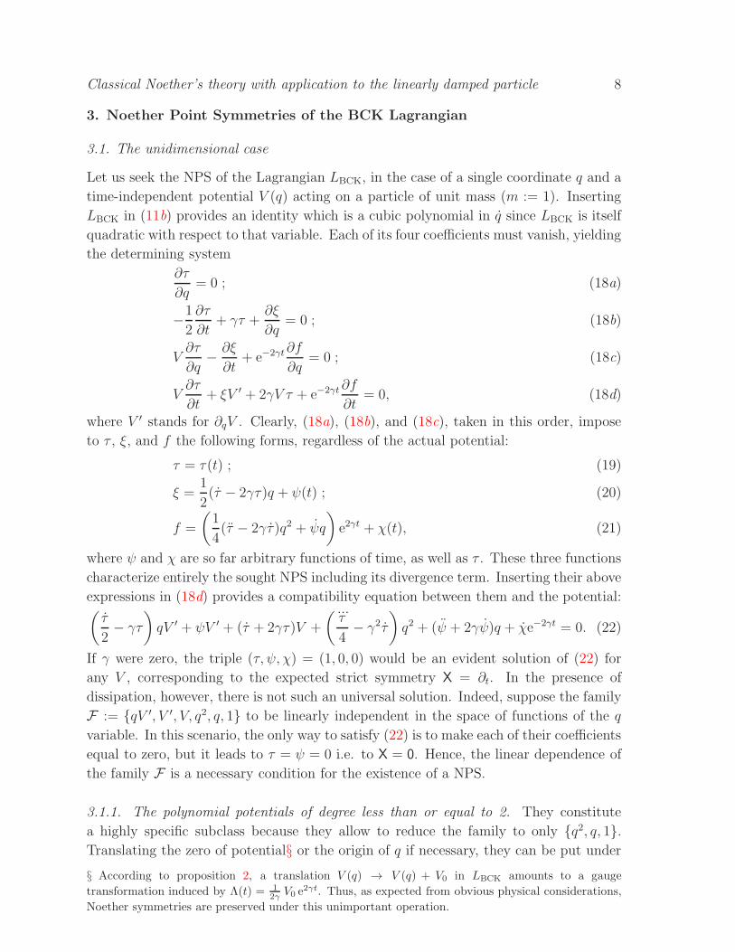
Let us seek the NPS of the Lagrangian LBCK, in the case of a single coordinate q and a
time-independent potential V (q) acting on a particle of unit mass (m := 1). Inserting
LBCK in (11b) provides an identity which is a cubic polynomial in q since LBCK is itself
quadratic with respect to that variable. Each of its four coefficients must vanish, yielding
the determining system
∂τ
∂q= 0 ; (18a)
−1
2
∂τ
∂t+ γτ +
∂ξ
∂q= 0 ; (18b)
V∂τ
∂q− ∂ξ
∂t+ e−2γt∂f
∂q= 0 ; (18c)
V∂τ
∂t+ ξV ′ + 2γV τ + e−2γt ∂f
∂t= 0, (18d)
where V ′ stands for ∂qV . Clearly, (18a), (18b), and (18c), taken in this order, impose
to τ , ξ, and f the following forms, regardless of the actual potential:
τ = τ(t) ; (19)
ξ =1
2(τ − 2γτ)q + ψ(t) ; (20)
f =
(1
4(τ − 2γτ)q2 + ψq
)e2γt + χ(t), (21)
where ψ and χ are so far arbitrary functions of time, as well as τ . These three functions
characterize entirely the sought NPS including its divergence term. Inserting their above
expressions in (18d) provides a compatibility equation between them and the potential:(τ
2− γτ
)qV ′ + ψV ′ + (τ + 2γτ)V +
( ...τ
4− γ2τ
)q2 + (ψ + 2γψ)q + χe−2γt = 0. (22)
If γ were zero, the triple (τ, ψ, χ) = (1, 0, 0) would be an evident solution of (22) for
any V , corresponding to the expected strict symmetry X = ∂t. In the presence of
dissipation, however, there is not such an universal solution. Indeed, suppose the family
F := qV ′, V ′, V, q2, q, 1 to be linearly independent in the space of functions of the q
variable. In this scenario, the only way to satisfy (22) is to make each of their coefficients
equal to zero, but it leads to τ = ψ = 0 i.e. to X = 0. Hence, the linear dependence of
the family F is a necessary condition for the existence of a NPS.
3.1.1. The polynomial potentials of degree less than or equal to 2. They constitute
a highly specific subclass because they allow to reduce the family to only q2, q, 1.Translating the zero of potential§ or the origin of q if necessary, they can be put under
§ According to proposition 2, a translation V (q) → V (q) + V0 in LBCK amounts to a gauge
transformation induced by Λ(t) = 12γ V0 e
2γt. Thus, as expected from obvious physical considerations,
Noether symmetries are preserved under this unimportant operation.
Classical Noether’s theory with application to the linearly damped particle 9
Noether point symmetry First integral Divergence term
X1 = ∂q I1 = 12γ
(2γq − F
)e2γt f1 = F
2γ e2γt
X2 = e−2γt∂q I2 = Ft− 2γq − q f2 = Ft− 2γq
X3 = e2γt(2γ∂t + F∂q
)I3 = γI21 f3 = F
4γ
(8γ2q + F
)e4γt
X4 = e−2γt(∂t + (Ft− 2γq)∂q
)I4 = 1
2 I22 f4 = 2γ2q2 + Fq(1− 2γt) + 1
2F2t2
X5 = 2∂t + (Ft− 2γq)∂q I5 = I1(I2 − F
2γ
)f5 = F
4γ2
(F (2γt− 1) + 4γ2q
)e2γt
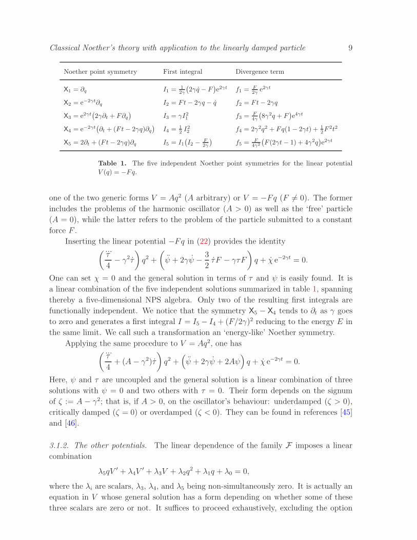
Table 1. The five independent Noether point symmetries for the linear potential
V (q) = −Fq.
one of the two generic forms V = Aq2 (A arbitrary) or V = −Fq (F 6= 0). The former
includes the problems of the harmonic oscillator (A > 0) as well as the ‘free’ particle
(A = 0), while the latter refers to the problem of the particle submitted to a constant
force F .
Inserting the linear potential −Fq in (22) provides the identity( ...τ
4− γ2τ
)q2 +
(ψ + 2γψ − 3
2τF − γτF
)q + χ e−2γt = 0.
One can set χ = 0 and the general solution in terms of τ and ψ is easily found. It is
a linear combination of the five independent solutions summarized in table 1, spanning
thereby a five-dimensional NPS algebra. Only two of the resulting first integrals are
functionally independent. We notice that the symmetry X5 − X4 tends to ∂t as γ goes
to zero and generates a first integral I = I5 − I4 + (F/2γ)2 reducing to the energy E in
the same limit. We call such a transformation an ‘energy-like’ Noether symmetry.
Applying the same procedure to V = Aq2, one has( ...τ
4+ (A− γ2)τ
)q2 +
(ψ + 2γψ + 2Aψ
)q + χ e−2γt = 0.
Here, ψ and τ are uncoupled and the general solution is a linear combination of three
solutions with ψ = 0 and two others with τ = 0. Their form depends on the signum
of ζ := A − γ2; that is, if A > 0, on the oscillator’s behaviour: underdamped (ζ > 0),
critically damped (ζ = 0) or overdamped (ζ < 0). They can be found in references [45]
and [46].
3.1.2. The other potentials. The linear dependence of the family F imposes a linear
combination
λ5qV′ + λ4V
′ + λ3V + λ2q2 + λ1q + λ0 = 0,
where the λi are scalars, λ3, λ4, and λ5 being non-simultaneously zero. It is actually an
equation in V whose general solution has a form depending on whether some of these
three scalars are zero or not. It suffices to proceed exhaustively, excluding the option
Classical Noether’s theory with application to the linearly damped particle 10
V1(q) = A log(q) V2(q) = Aqα + 4γ2α
(α+2)2 q2 V3(q) = Aeq + 8γ2q
X e−2γt(∂t − 2γq∂q
)e2γ
α−2
α+2t(∂t − 4γ
α+2q∂q)
e2γt(∂t − 4γ∂q
)
f 2γ(γq2 +At) 4γ2(2−α)(α+2)2 q2e
4γα
α+2t 8γ2(1 − q)e4γt
I 12 (q + 2γq)2 +A log(q) + 2γAt
(12 (q +
4γα+2q)
2 +Aqα)e
4γα
α+2t
(12 (q + 4γ)2 +Aeq
)e4γt
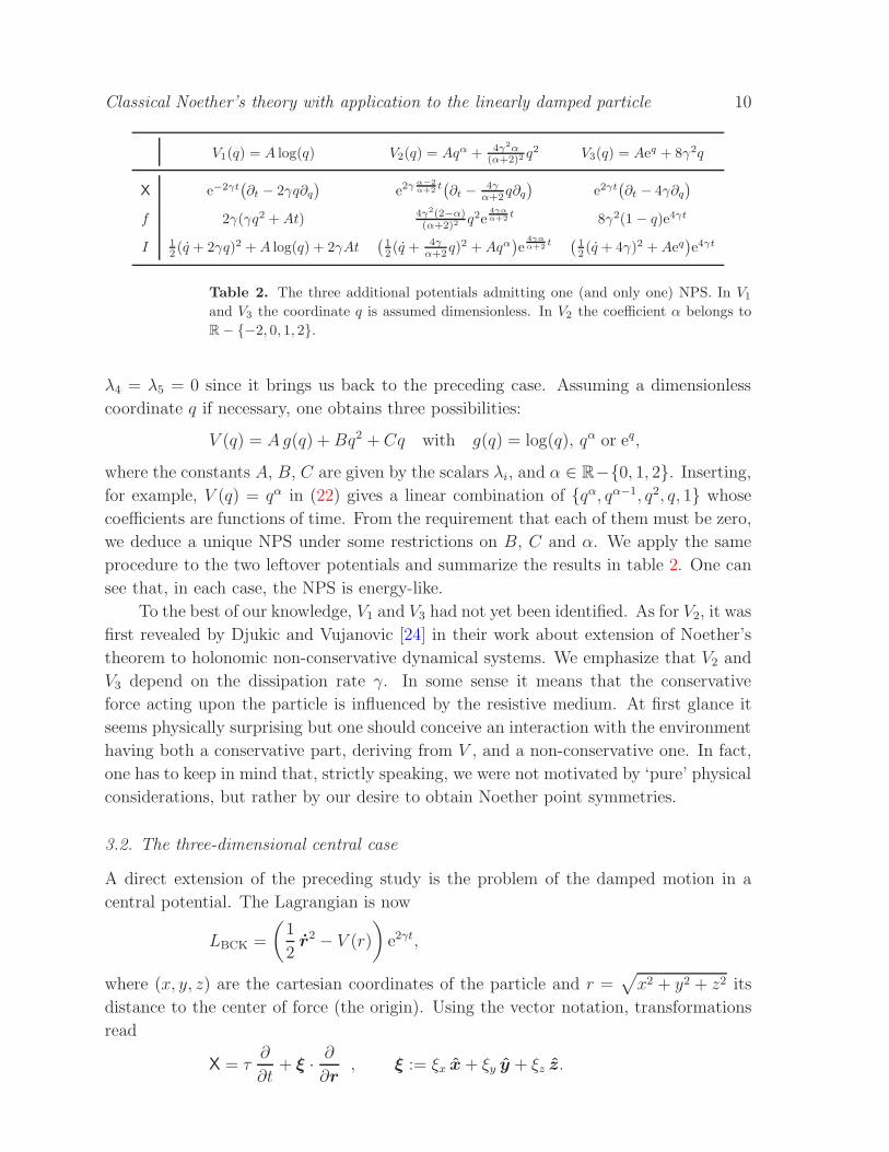
Table 2. The three additional potentials admitting one (and only one) NPS. In V1
and V3 the coordinate q is assumed dimensionless. In V2 the coefficient α belongs to
R− −2, 0, 1, 2.
λ4 = λ5 = 0 since it brings us back to the preceding case. Assuming a dimensionless
coordinate q if necessary, one obtains three possibilities:
V (q) = Ag(q) +Bq2 + Cq with g(q) = log(q), qα or eq,
where the constants A, B, C are given by the scalars λi, and α ∈ R−0, 1, 2. Inserting,for example, V (q) = qα in (22) gives a linear combination of qα, qα−1, q2, q, 1 whose
coefficients are functions of time. From the requirement that each of them must be zero,
we deduce a unique NPS under some restrictions on B, C and α. We apply the same
procedure to the two leftover potentials and summarize the results in table 2. One can
see that, in each case, the NPS is energy-like.
To the best of our knowledge, V1 and V3 had not yet been identified. As for V2, it was
first revealed by Djukic and Vujanovic [24] in their work about extension of Noether’s
theorem to holonomic non-conservative dynamical systems. We emphasize that V2 and
V3 depend on the dissipation rate γ. In some sense it means that the conservative
force acting upon the particle is influenced by the resistive medium. At first glance it
seems physically surprising but one should conceive an interaction with the environment
having both a conservative part, deriving from V , and a non-conservative one. In fact,
one has to keep in mind that, strictly speaking, we were not motivated by ‘pure’ physical
considerations, but rather by our desire to obtain Noether point symmetries.
3.2. The three-dimensional central case
A direct extension of the preceding study is the problem of the damped motion in a
central potential. The Lagrangian is now
LBCK =
(1
2r2 − V (r)
)e2γt,
where (x, y, z) are the cartesian coordinates of the particle and r =√x2 + y2 + z2 its
distance to the center of force (the origin). Using the vector notation, transformations
read
X = τ∂
∂t+ ξ · ∂
∂r, ξ := ξx x+ ξy y + ξz z.
Classical Noether’s theory with application to the linearly damped particle 11
The Killing-type equation (11b) thereby obtained is yet again a cubic polynomial in
velocities. The cubic, quadratic and linear monomials, taken one by one, provide the
following forms for τ , ξ and f :
τ = τ(t) ;
ξ =1
2(τ − 2γτ) r +α× r +ψ(t) ;
f =
(1
4(τ − 2γτ) r2 + ψ · r
)e2γt + χ(t),
where α is a constant vector and ψ a time-dependent one. Then, the monomial of
degree zero imposes the compatibility condition(τ
2− γτ
)rV ′+(τ+2γτ)V +
( ...τ
4− γ2τ
)r2+ χ e−2γt = −
(ψ + 2γ ψ +
V ′
rψ
)·r.(23)
Vector α does not appear in (23). Consequently, whatever α be, the transformation
X = (α× r) · ∂∂r
(24)
is a strict NPS of the Lagrangian, irrespective of the central potential V . It is the
generator of the rotation of magnitude ‖α‖ around the direction-vector α. In other
words, LBCK is rotationally invariant, as expected by the isotropic nature of both the
conservative force and the dissipation. The transformation (24) generates the first
integral
I(α) = (α× r) · ∂LBCK
∂r= α · (r × r) e2γt.
Since it is true for any α, one obtains the conservation of
ℓ0 = (r × r) e2γt = ℓ e2γt,where ℓ is the angular momentum about the origin, equals to ℓ0 at t = 0. As a
corollary, the motion takes place in the plane (through the origin) orthogonal to the
constant vector ℓ0, with an areal velocity decreasing exponentially with time.
Let us seek eventual supplementary symmetries. Passing to the spherical
coordinates (r, ϑ, ϕ), such that
x = r sinϑ cosϕ , y = r sinϑ sinϕ , z = r cosϑ,
the left-hand side of (23) has a spatial dependence contained only in the variable r,
while the other side depends also on the two angles. Differentiating that equation two
times with respect to ϑ, the LHS disappears whereas the RHS changes sign. Hence, the
latter must be zero as well as the former and (23) splits into two:(τ
2− γτ
)rV ′ + (τ + 2γτ)V +
( ...τ
4− γ2τ
)r2 + χ e−2γt = 0 ; (25)
ψ + 2γ ψ +V ′
rψ = 0. (26)
Equation (26) can only be fulfilled by quadratic (or zero) potentials V = Ar2. Actually,
these potentials are very special since they make LBCK separable into three replications of
Classical Noether’s theory with application to the linearly damped particle 12
the same one-dimensional Lagrangian, each one in terms of a single cartesian coordinate.
Hence, these peculiar cases bring us back to the previous problem and contain 3×5 = 15
NPS in all.
The non-quadratic potentials, however, must verify equation (25) which is quite
similar to (22) but differs by the absence of the function ψ. Consequently, the solutions
of (23) are exactly the ones of (22) having a zero ψ (after replacing q by r). A quick
inspection of tables 1 and 2 shows that V1 and V2 have an additional symmetry, in
contrary to V3 and the linear potential.
4. From Noether point symmetries to equivalent autonomous problems
As a rule in physics, a symmetry provides suitable coordinates for the description of a
problem in a simpler way. Having this idea in mind, we will show how such coordinates
arise from a NPS, and secondly how they can be used to map a general Lagrangian
problem into an autonomous one, whose Hamiltonian is precisely the first integral I
generated by the symmetry. Then, we will apply the procedure to LBCK.
Let L be any Lagrangian in terms of n coordinates qi, and suppose that it possesses
the NPS
X = τ(q, t)∂
∂t+ ξi(q, t)
∂
∂qi,
with divergence term f . Since we will perform changes of variables, it seems preferable
to use more intrinsic formulations. First, noticing that X(t) = τ and X(qi) = ξi, the
NPS may be written
X = X(t)∂
∂t+ X(qi)
∂
∂qi.
Then, using the total time-derivative operator (10), the Rund-Trautman identity (7)
verified by X becomes
X[1](L) + D(X(t))L = D(f). (27)
Now, let us consider an invertible change of variables (q, t) → (Q, T ), where Q is seen
as the new set of coordinates and T the new time. It provides an alternative expression
to the vector field X:
X = X(T )∂
∂T+ X(Qi)
∂
∂Qi.
To avoid any confusion, we denote the total derivative with respect to T in this new
representation by the ‘prime’ symbol, the corresponding operator being
D = ∂T +Qi′ ∂
∂Qi+ . . . = D(t)D.
The dynamics in the (Q, T ) variables may now be described by the transformed
Lagrangian
L(Q,Q′, T ) = L D(t).
Classical Noether’s theory with application to the linearly damped particle 13
Here, the identity (12) is equivalent to
D(X(G))− X[1](D(G)) = D(X(T ))D(G), (28)
for any function G defined over the extended configuration space. Using (28) with G ≡ t,
one readily derives from (27)
X[1](L) + D(X(T ))L = D(t)
[X[1](L) + D(X(t))L
]= D(t)D(f) = D(f).
In words, X remains a NPS of L, with the same divergence term. The corresponding
first integral, as logic suggests, is still I (see the appendix):
I = f − LX(T )− ∂L
∂Qi′
(X(Qi)−Qi′
X(T ))= I. (29)
The variables (Q, T ) are so far arbitrary but, in order to take into account the symmetry
in the simplest possible way, one has to choose proper ones. They are the canonical
variables of X, such that X(Qi) = 0 and X(T ) = 1. They reduce X to the translation
symmetry ∂T . Performing a gauge change if necessary, thanks to proposition 2 and
formula (13), one has thereby obtained a Lagrangian which is T -independent. All this
can be summarized in the following theorem.
Theorem 4 Let (Q, T ) be canonical variables of X, such that X(Qi) = 0 and X(T ) = 1,
and let Λ be a function satisfying the gauge condition f + X(Λ) = 0. Then, in the
(Q, T ) variables, the new Lagrangian L = L D(t) + D(Λ) is explicitly T -independent:
L = L(Q,Q′). Furthermore, the induced Hamiltonian is precisely the first integral I:
H = PiQi′ − L = I with Pi =
∂L
∂Qi ′.
Let us apply the theorem to LBCK in one dimension for which we assume a NPS
with a nonzero τ function. Taking advantage of the q-independence of τ , a simple time
rescaling t→ T is possible, through
T =
∫dt
τ.
To obtain the canonical coordinate Q, we seek an invariant of the differential equation
dt
τ=
dq
ξ,
with ξ given by (20). One easily finds
Q =eγt√τq −
∫eγtψ
τ 3/2dt.
The new velocity is thus given by
Q′ =D(Q)
D(T )= τ
(∂Q
∂t+ q
∂Q
∂q
)= eγt
√τ
(q − ξ
τ
). (30)
Hereafter Q and T are the independent variables. Since f is quadratic in q which is
itself linear in Q, the function f has the form
f = f2(T )Q2 + f1(T )Q+ f0(T ).
Classical Noether’s theory with application to the linearly damped particle 14
Expanding (21) gives the precise expressions of f0, f1, and f2. In particular, the last
two ones are
f1 =1
2(τ − 2γτ ) τ
∫eγtψ
τ 3/2dt + ψ eγt
√τ ;
f2 =1
4(τ − 2γτ ) τ.
The gauge condition f + X(Λ) = f + ∂TΛ = 0 is automatically fulfilled if one sets
Λ = −Q2
∫f2(T ) dT −Q
∫f1(T ) dT −
∫f0(T ) dT.
However, the construction of the explicitly T -independent Lagrangian needs only the
knowledge of D(Λ), that is, the partial derivatives of Λ. The first one, ∂TΛ = −f , isalready known and the integration of f1 and f2 yields
∂Λ
∂Q= −2Q
∫f2(T ) dT −
∫f1(T ) dT = − ξ√
τeγt.
Then, using (30), the autonomous Lagrangian is
L(Q,Q′) = L D(t) + D(Λ) =1
2Q′2 − V (Q), (31)
where
V =
(V τ − ξ2
2τ
)e2γt + f
appears as the new potential. For consistency, one can check the T -independence of V :
∂V
∂T= X(V ) = τ
∂V
∂t+ ξ
∂V
∂q= 0,
by virtue of equations (18a)-(18d). As a last step, we derive from (31) the momentum
P = Q′ and the conserved Hamiltonian
H(Q,P ) =1
2P 2 + V (Q) = I.
In this new picture, I is nothing but the energy of the equivalent autonomous problem.
We summarize on table 3 the explicit transformations together with their associated
Hamiltonian for the three potentials V1, V2, and V3 found above. We also include the
case of the linear potential −Fq whose three symmetries X3, X4, X5 have a nonzero τ
(see table 1). Finally, applying also theorem 4 to the NPS whose τ is zero, we end
table 3 with the two leftover NPS of the linear potential. The same procedure may be
followed in the three-dimensional central case as well.
5. Lie point symmetries
A Noether symmetry of a Lagrangian L has the well-known property of permuting
solutions of the Euler-Lagrange equations. In other words, it is a Lie symmetry of these
equations:
X[2](Ei(L)) = 0 when Ej(L) = 0, (32)
Classical Noether’s theory with application to the linearly damped particle 15
V T Q H
V1(q) = A log(q) 12γ e2γt q e2γt 1
2P2 +A log(Q)
V2(q) = Aqα + 4γ2α(α+2)2
q2 12γ
2+α2−α e2γ
2−α2+α
tq e
4γt
α+2 12P
2 +AQα
V3(q) = Aeq + 8γ2q − 12γ e−2γt q + 4γt 1
2P2 +AeQ
(X3) e−2γt 2γq − Ft 12 P
2
(X4) e2γt (F (1− 2γt) + 4γ2q) e2γt 12P
2
V (q) = −Fq (X5) γt (F (1− γt) + 2γ2q) eγt 12P
2 − 12Q
2
(X1) 2γ2q e2γt (2√P + F )Q
(X2)γ2
2 qe2γt γt 2e−Q√P + FQ
Table 3. Autonomous one-dimensional Hamiltonians deduced from the symmetries.
where we introduced the second prolongation of X:
X[2] := X
[1] + (ξ i − qiτ − 2q iτ )∂
∂q i.
The converse is not true, in general. For instance, ∂t is basically a Lie symmetry of
E(LBCK) = 0 whatever V (q) be but it is never a Noether symmetry of LBCK. Thus,
one expects more symmetries by seeking solutions of (32) and, by the way, more first
integrals.
Yet again, let us restrict ourself to Lie point symmetries (LPS) in one dimension.
Each of them ‘carries’ naturally a first integral which may be extracted as follows. We
first determine a zero order x = x(q, t) and a first order y = y(q, q, t) invariants of X[1].
Then, according to Lie’s theory, the second order differential equation E(L) = 0 may be
reduced to a first order one, say Φ(x, y, y′x) = 0, with
y′x :=D(y)
D(x).
Its general solution admits an implicit form G(x, y) = C, where C is an integration
constant; whence,
I(q, q, t) := G(x(q, t), y(q, q, t)) = cst. when E(L) = 0.
Since G is a function of X’s invariants, I is also an invariant of the LPS, i.e. X[1](I) = 0.
Applying the method to the LPS ∂t of the Euler-Lagrange equation derived from LBCK,
with x = q and y = q, one obtains an Abel equation of the second kind, viz.
yy′x + 2γy + ∂xV (x) = 0.
It must be solved to deduce the first integral, which has the great advantage of being
explicitly time-independent. The other side of the coin is that it is generally a hard task
which necessitates tedious algebraic and analytic manipulations to obtain cumbersome
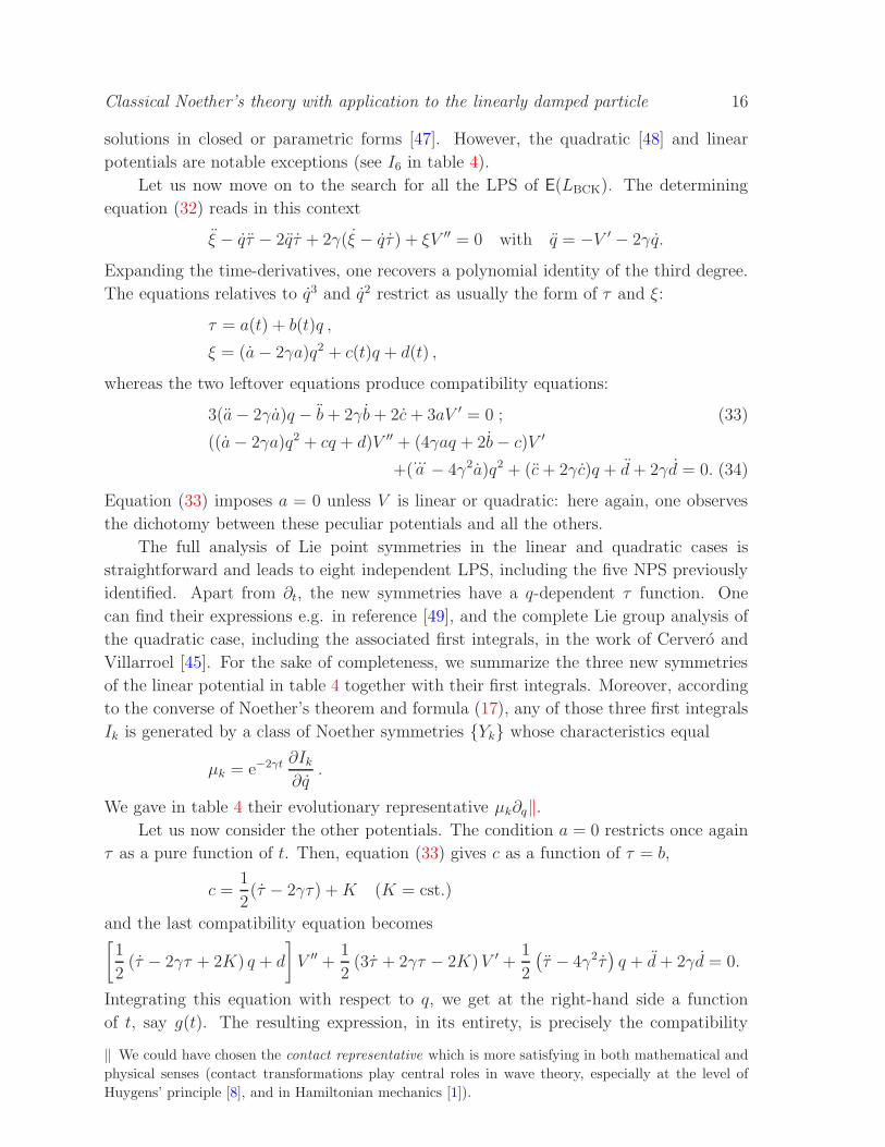
Classical Noether’s theory with application to the linearly damped particle 16
solutions in closed or parametric forms [47]. However, the quadratic [48] and linear
potentials are notable exceptions (see I6 in table 4).
Let us now move on to the search for all the LPS of E(LBCK). The determining
equation (32) reads in this context
ξ − qτ − 2qτ + 2γ(ξ − qτ ) + ξV ′′ = 0 with q = −V ′ − 2γq.
Expanding the time-derivatives, one recovers a polynomial identity of the third degree.
The equations relatives to q3 and q2 restrict as usually the form of τ and ξ:
τ = a(t) + b(t)q ,
ξ = (a− 2γa)q2 + c(t)q + d(t) ,
whereas the two leftover equations produce compatibility equations:
3(a− 2γa)q − b+ 2γb+ 2c+ 3aV ′ = 0 ; (33)
((a− 2γa)q2 + cq + d)V ′′ + (4γaq + 2b− c)V ′
+(...a − 4γ2a)q2 + (c+ 2γc)q + d+ 2γd = 0. (34)
Equation (33) imposes a = 0 unless V is linear or quadratic: here again, one observes
the dichotomy between these peculiar potentials and all the others.
The full analysis of Lie point symmetries in the linear and quadratic cases is
straightforward and leads to eight independent LPS, including the five NPS previously
identified. Apart from ∂t, the new symmetries have a q-dependent τ function. One
can find their expressions e.g. in reference [49], and the complete Lie group analysis of
the quadratic case, including the associated first integrals, in the work of Cervero and
Villarroel [45]. For the sake of completeness, we summarize the three new symmetries
of the linear potential in table 4 together with their first integrals. Moreover, according
to the converse of Noether’s theorem and formula (17), any of those three first integrals
Ik is generated by a class of Noether symmetries Yk whose characteristics equal
µk = e−2γt ∂Ik∂q
.
We gave in table 4 their evolutionary representative µk∂q‖.Let us now consider the other potentials. The condition a = 0 restricts once again
τ as a pure function of t. Then, equation (33) gives c as a function of τ = b,
c =1
2(τ − 2γτ) +K (K = cst.)
and the last compatibility equation becomes[1
2(τ − 2γτ + 2K) q + d
]V ′′ +
1
2(3τ + 2γτ − 2K)V ′ +
1
2
(τ − 4γ2τ
)q + d+ 2γd = 0.
Integrating this equation with respect to q, we get at the right-hand side a function
of t, say g(t). The resulting expression, in its entirety, is precisely the compatibility
‖ We could have chosen the contact representative which is more satisfying in both mathematical and
physical senses (contact transformations play central roles in wave theory, especially at the level of
Huygens’ principle [8], and in Hamiltonian mechanics [1]).
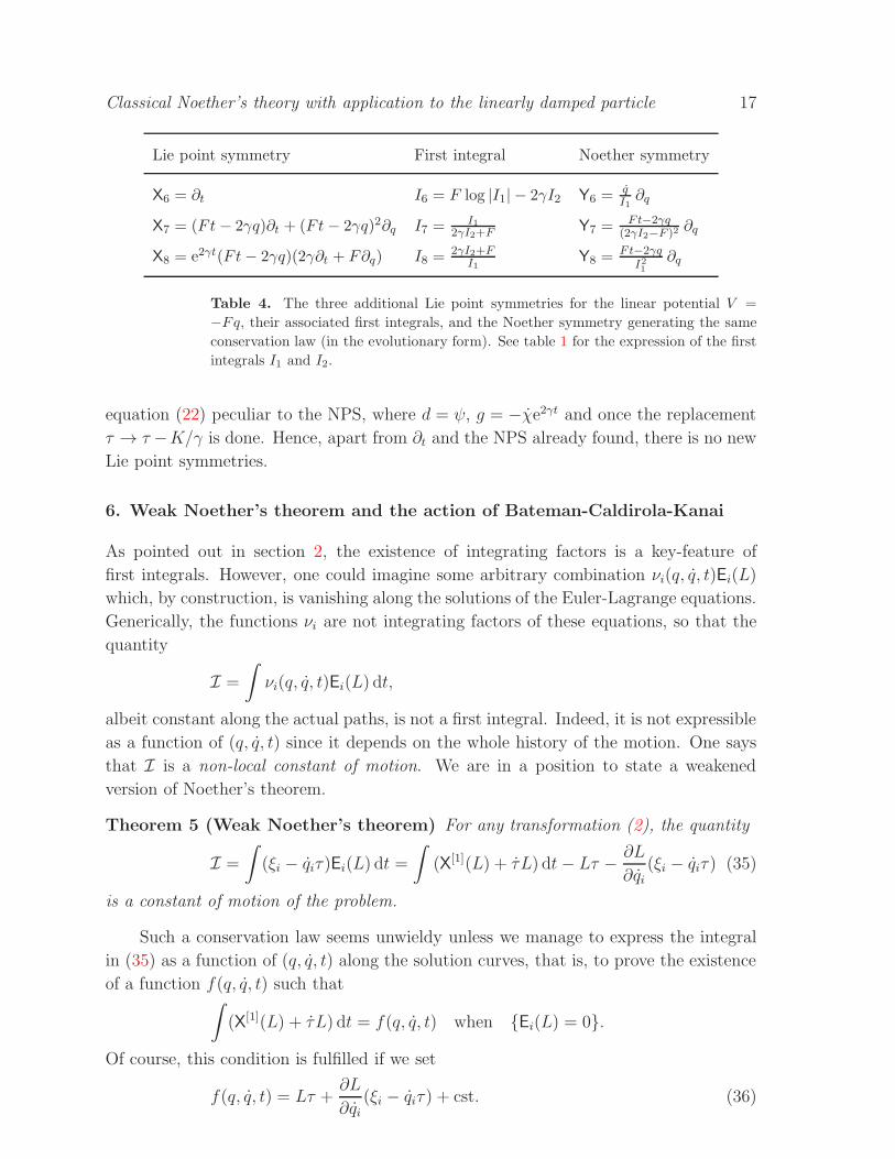
Classical Noether’s theory with application to the linearly damped particle 17
Lie point symmetry First integral Noether symmetry
X6 = ∂t I6 = F log |I1| − 2γI2 Y6 =qI1∂q
X7 = (Ft− 2γq)∂t + (Ft− 2γq)2∂q I7 =I1
2γI2+F Y7 =Ft−2γq
(2γI2−F )2∂q
X8 = e2γt(Ft− 2γq)(2γ∂t + F∂q) I8 =2γI2+F
I1Y8 =
Ft−2γqI21
∂q
Table 4. The three additional Lie point symmetries for the linear potential V =
−Fq, their associated first integrals, and the Noether symmetry generating the same
conservation law (in the evolutionary form). See table 1 for the expression of the first
integrals I1 and I2.
equation (22) peculiar to the NPS, where d = ψ, g = −χe2γt and once the replacement
τ → τ −K/γ is done. Hence, apart from ∂t and the NPS already found, there is no new
Lie point symmetries.
6. Weak Noether’s theorem and the action of Bateman-Caldirola-Kanai
As pointed out in section 2, the existence of integrating factors is a key-feature of
first integrals. However, one could imagine some arbitrary combination νi(q, q, t)Ei(L)
which, by construction, is vanishing along the solutions of the Euler-Lagrange equations.
Generically, the functions νi are not integrating factors of these equations, so that the
quantity
I =
∫νi(q, q, t)Ei(L) dt,
albeit constant along the actual paths, is not a first integral. Indeed, it is not expressible
as a function of (q, q, t) since it depends on the whole history of the motion. One says
that I is a non-local constant of motion. We are in a position to state a weakened
version of Noether’s theorem.
Theorem 5 (Weak Noether’s theorem) For any transformation (2), the quantity
I =
∫(ξi − qiτ)Ei(L) dt =
∫(X[1](L) + τL) dt− Lτ − ∂L
∂qi(ξi − qiτ) (35)
is a constant of motion of the problem.
Such a conservation law seems unwieldy unless we manage to express the integral
in (35) as a function of (q, q, t) along the solution curves, that is, to prove the existence
of a function f(q, q, t) such that∫(X[1](L) + τL) dt = f(q, q, t) when Ei(L) = 0.
Of course, this condition is fulfilled if we set
f(q, q, t) = Lτ +∂L
∂qi(ξi − qiτ) + cst. (36)
Classical Noether’s theory with application to the linearly damped particle 18
but such a naive choice leads to a truism: scalar numbers are constants of motion.
Actually, any alternative expression f(q, q, t) provides a true first integral (this is
certainly the case if f does not depend on q). It amounts to ask for a function f ,
excluding (36), such that
X[1](L) + τL = f when Ei(L) = 0.
Put another way, the transformation X must be an ‘on-flow’ solution of the Rund-
Trautman identity. We mention that, recently, Gorni and Zampieri [44, 50] used this
weakened Noether’s theorem to derive alternative constructions of some known first
integrals.
The theorem gives us access to non-local extensions of the usual conservation laws.
For instance, the time translation ∂t is a Noether symmetry if and only if, according
to (16), µi = qi are integrating factors. When L is time-independent, this is certainly the
case and the corresponding first integral is the Hamiltonian H = qi∂qiL−L. Generally,
it comes down to the law of conservation of mechanical energy. On the contrary, if ∂t is
not a Noether symmetry one can nonetheless associate to ∂t the constant of motion
I = −∫qi Ei(L) dt = H +
∫∂L
∂tdt.
It reflects basically the relation ∂tL = −H along the solution curves. Returning to LBCK,
this constant of motion acquires an interesting physical meaning. Indeed, noticing the
singular property
∂LBCK
∂t= 2γ LBCK,
one obtains the kinematic conservation of
I = H + 2γABCK, (37)
where
ABCK =
∫LBCK dt
is the action based on LBCK. Consequently, along the solution curves, the action is
expressible as a function of (r, r, t):
ABCK =I −H
2γwhen E(LBCK) = 0, (38)
where I plays merely the role of an integrating constant. Now, suppose that one manages
to find an alternative expression of ABCK, i.e. a function G(r, r, t) such that
ABCK = G(r, r, t) 6≡ −H
2γ+ cst. when E(LBCK) = 0.
Then, by injecting this expression in (37), I becomes a non-trivial first integral I.
Conversely, if I is so, one extracts from (38) an expression of ABCK along the solution
curves. To sum up, an alternative local expression of the action along the actual

Classical Noether’s theory with application to the linearly damped particle 19
paths amounts to a first integral, i.e. to a Noether symmetry. According to (9), this
relationship is given by
ABCK =1
2γ
[f − (1 + τ)
(1
2r2 + V
)e2γt − ξ · r e2γt
],
where τ is chosen dimensionless.
7. Conclusion
In this article, we addressed the question of the conservation laws in the classical
dynamics of a particle submitted to a linear dissipation, basing our study on the
variational framework offered by the celebrated BCK Lagrangian. We found all the time-
independent potentials V (q) for which the Lagrangian admits Noether point symmetries
in the unidimensional case. Then, we showed that not all of them ‘resist’ under the
direct mapping V (q) → V (r) to the central case in three dimensions. As a next stage,
we established a systematic method to transform Lagrangians enjoying a variational
point symmetry into autonomous others, and applied it in our context. For the sake of
completeness, we also investigated the Lie point symmetries which form an overalgebra
of Noether ones. Apart from the family of potentials at most quadratic, whose point
symmetry algebra gains three dimensions (from 5 to 8), the others acquire only the
obvious time translation symmetry. Finally, we enlightened the interconnection between
symmetries and the BCK action functional, in relation with a weakened version of
Noether’s theorem and the idea of on-flow solutions of the Rund-Trautman identity.
Acknowledgments
We wish to thank all the colleagues of the Groupe de Physique Statistique for many
enlightening discussions. One of us (R. L.) is grateful for their kind hospitality.
Appendix
We give here a simple proof of formula (29). Using the hypothesis and notations of
section 4, the equality L = LD(t), i.e. Ldt = LdT , is tantamount to the invariance of
the Poincare-Cartan form, that is
pidqi −Hdt = PidQ
i − HdT.
Setting q0 = t, p0 = −H , Q0 = T , P0 = −H , this invariance reads
pµdqµ = PµdQ
µ , (A.1)
where the index µ goes from 0 to n. Furthermore, the first integrals I and I induced by
the common point symmetry X of L and L become simply
I = f − pµ X(qµ) and I = f − Pµ X(Q
µ).
REFERENCES 20
The equality (A.1) allows to determine the new momenta from the old ones through
pν∂qν
∂QµdQµ = PµdQ
µ =⇒ Pµ = pν∂qν
∂Qµ. (A.2)
Then,
I = f − pν∂qν
∂QµX(Qµ) = f − pνX(q
ν) = I.
This result is nothing else but the scalar nature of pµ X(qµ) inherited from the covariance
of the momenta pµ and the contravariance of the coordinates qµ.
References
[1] Whittaker E T 1959 A treatrise on the analytical dynamics of particles and rigid
bodies (New-York: Cambridge Univ. Press)
[2] Goldstein H 1980 Classical mechanics (Reading, Massachusetts: Addison-Wesley)
[3] Neuenschwander D E 2011 Emmy Noether’s wonderful theorem (Baltimore: The
John Hopkins University Press)
[4] Noether E 1918 Ges. Wiss. Gottingen 2 235
[5] Sarlet W and Cantrijn F 1981 SIAM Rev. 23 467
[6] Lie S 1891 Vorlesungen uber Differenrialgleichungen mit Bekannten Infinitesimalen
Transformationen (Leipzig: B. G. Teubner)
[7] Olver P J 1986 Application of Lie groups to differential equations (New-York:
Springer)
[8] Ibragimov N H 1992 Russ. Math. Surv. 47 89
[9] Muriel C and Romero J L 2001 IMA J. Appl. Math. 66 111
[10] Muriel C and Romero J L 2003 J. Lie Theory 13 167
[11] Jacobi C G J 1842 C. R. Acad. Sci. Paris 15 202
[12] Jacobi C G J 1866 Vorlesungen uber Dynamik (Berlin: G. Reimer)
[13] Nucci M C and Leach P G L 2008 Phys. Scr. 78 0065011
[14] Duarte L G, Duarte S E S, da Mota L A C P and F S J E 2001 J. Phys. A: Math.
Gen. 34 3014
[15] Anco S C and Bluman G 1998 Eur. J. Appl. Math. 9 245
[16] Cheb-Terrab E S and Roche A D 1999 J. Symbol. Comput. 27 501
[17] Nucci M C 2005 J. Math. Phys. 12 284
[18] Muriel C and Romero J L 2009 J. Phys. A: Math. Gen. 42 365207
[19] Mohanasubha R, Chandrasekar V K, Senthilvelan M and Lakshmanan M 2014
Proc. R. Soc. A 470 20130656
[20] Nucci M C and Levi D 2013 Nonlin. Anal. RWA 14 1092
[21] Helmholtz H 1887 J. Reine Angew. Math. 100 137
REFERENCES 21
[22] Havas P 1957 Nuovo Cimento Suppl. 5 363
[23] Nucci M C and Leach P G L 2008 J. Math. Phys. 49 073517
[24] Djukic D S and Vujanovic B D 1975 Acta Mech. 23 17
[25] Vujanovic B D 1978 Int. J. Nonl. Mech. 13 185
[26] Bateman H 1931 Phys. Rev. 38 815
[27] Caldirola P 1941 Nuovo Cimento 18 393
[28] Kanai E 1948 Prog. Theor. Phys. 3 440
[29] Denman H H 1966 Am. J. Phys. 34 1147
[30] Denman H H and Buch L W 1972 J. Math. Phys. 47 857
[31] Lemos N A 1979 Am. J. Phys. 47 857
[32] Bahar L Y and Kwatny H G 1981 Am. J. Phys. 49 1062
[33] Kobe D H, Reali G and Sieniutycz S 1986 Am. J. Phys. 54 997
[34] Ares-de-Parga G, Rosales M A and Jimenez J L 1989 Am. J. Phys. 57 941
[35] Razavy M 2005 Classical and quantum dissipative systems (London: Imperial
College Press)
[36] Kerner E H 1958 Can. J. Phys. 36 371
[37] Senitzky I R 1960 Phys. Rev. 119 670
[38] Dekker H 1981 Phys. Rep. 80 1
[39] Baldiotti M C, Fresneda R and Gitman D M 2011 Phys. Lett. A 375 1630
[40] Mahomed F M, Kara A H and Leach P G L 1993 J. Math. Anal. Appl. 178 116
[41] Bessel-Hagen E 1921 Math. Ann. 84 258
[42] Rund H 1972 Util. Math 2 205
[43] Trautman A 1967 Commun. Math. Phys. 6 248
[44] Gorni G and Zampieri G 2014 (Preprint 1403.0506)
[45] Cervero J M and Villarroel J 1984 J. Phys. A: Math. Gen. 17 1777
[46] Choudhuri A, Ghosh J and Talukdar B 2008 Pramana J. Phys. 70 657
[47] Polyanin A D and Zaitsev V F 1995 Handbook of Exact Solutions for Ordinary
Differential Equations (New-York: CRC Press)
[48] Denman H H 1968 Am. J. Phys. 36 516
[49] Pandey S N, Bindu P, Senthilvelan M and Lakshmanan 2009 J. Math. Phys. 50
102701
[50] Gorni G and Zampieri G 2014 J. Nonlinear Math. Phys. 21 43


![Some applications of Noether’s theorem · admits a variational symmetry [32], hence we apply the Noether’s theorem in the Lanczos approach to prove that the corresponding conserved](https://img.pdfslide.net/doc/110x75/5ec1206b41f6c76c7d171954/some-applications-of-noetheras-admits-a-variational-symmetry-32-hence-we-apply.jpg)


![Gauge Invariant Noether’s Theorem and The Proton …arXiv:1802.02864v2 [hep-ph] 26 Feb 2018 Gauge Invariant Noether’s Theorem and The Proton Spin Crisis Gouranga C Nayak1,∗ 1](https://img.pdfslide.net/doc/110x75/5e607feaf36f191a1f5537c5/gauge-invariant-noetheras-theorem-and-the-proton-arxiv180202864v2-hep-ph-26.jpg)