KINEMATIC CALIBRATION OF INDUSTRIAL ROBOTS USING … · kinematic calibration of industrial robots using full pose measurements and optimal pose selection a thesis submitted to the

1

KINEMATIC CALIBRATION OF INDUSTRIAL ROBOTS USING FULL POSEMEASUREMENTS AND OPTIMAL POSE SELECTION

A THESIS SUBMITTED TOTHE GRADUATE SCHOOL OF NATURAL AND APPLIED SCIENCES

OFMIDDLE EAST TECHNICAL UNIVERSITY

BY

BERK YURTTAGUL

IN PARTIAL FULFILLMENT OF THE REQUIREMENTSFOR

THE DEGREE OF MASTER OF SCIENCEIN

MECHANICAL ENGINEERING

DECEMBER 2010

Approval of the thesis:

KINEMATIC CALIBRATION OF INDUSTRIAL ROBOTS USING FULL POSE

MEASUREMENTS AND OPTIMAL POSE SELECTION

submitted by BERK YURTTAGUL in partial fulfillment of the requirements for the degree ofMaster of Science in Mechanical Engineering Department, Middle East Technical Uni-versity by,

Prof. Dr. Canan OZGENDean, Graduate School of Natural and Applied Sciences

Prof. Dr. Suha ORALHead of Department, Mechanical Engineering

Asst. Prof. Dr. E. Ilhan KONUKSEVENSupervisor, Mechanical Engineering Dept., METU

Examining Committee Members:

Prof. Dr. Kemal OZGORENMechanical Engineering Dept., METU

Asst. Prof. Dr. E. Ilhan KONUKSEVENMechanical Engineering Dept., METU

Prof. Dr. Tuna BALKANMechanical Engineering Dept., METU

Asst. Prof. Dr.Bugra KOKUMechanical Engineering Dept., METU

Asst. Prof. Dr. Afsar SARANLIElectrical and Electronics Engineering Dept., METU

Date:

I hereby declare that all information in this document has been obtained and presentedin accordance with academic rules and ethical conduct. I also declare that, as requiredby these rules and conduct, I have fully cited and referenced all material and results thatare not original to this work.

Name, Last Name: BERK YURTTAGUL

Signature :

iii

ABSTRACT

KINEMATIC CALIBRATION OF INDUSTRIAL ROBOTS USING FULL POSEMEASUREMENTS AND OPTIMAL POSE SELECTION

Yurttagul, Berk

M.S., Department of Mechanical Engineering

Supervisor : Asst. Prof. Dr. E. Ilhan KONUKSEVEN

December 2010, 70 pages

This study focuses on kinematic calibration of industrial robots. Kinematic modeling, param-

eter identification and optimal pose selection methods are presented. A computer simulation

of the kinematic calibration is performed using generated measurements with normally dis-

tributed noise. Furthermore, kinematic calibration experiments are performed on an ABB

IRB 6600 industrial robot using full pose measurements taken by a laser tracking system.

The kinematic model of the robot is developed using the modified Denavit - Hartenberg con-

vention. A nonlinear least-squares method is employed during the parameter identification

stage. According to the experiment results, the initial robot positioning errors are reduced by

more than 80%.

Keywords: Kinematic Calibration, Parameter Identification, Industrial Robots

iv

OZ

ENDUSTRIYEL ROBOTLARIN TAM POZ OLCUMLERI VE ENIYILENMIS POZLARKULLANILARAK KINEMATIK KALIBRASYONU

Yurttagul, Berk

Yuksek Lisans, Makine Muhendisligi Bolumu

Tez Yoneticisi : Yrd. Doc. Dr. E. Ilhan KONUKSEVEN

Aralık 2010, 70 sayfa

Bu calısma endustriyel robotların kinematik kalibrasyonu uzerine odaklanmaktadır. Kine-

matik modelleme, parametre tanılama ve en iyi poz secimi yontemleri sunulmaktadır. Uretilen

normal dagılımlı gurultu iceren olcumler kullanılarak bilgisayar ortamında kinematik kali-

brasyon benzetimleri elde edildi. Bunun yanı sıra, tam poz olcumleri kullanılarak ABB IRB

6600 endustriyel robotu uzerinde kinematik kalibrasyon deneyleri gerceklestirildi. Robo-

tun kinematik modeli degistirilmis Denavit - Hartenberg notasyonu kullanılarak olusturuldu.

Parametre tanılama isleminde dogrusal olmayan kucuk kareler yontemi kullanıldı. Deney

sonuclarına gore robot konumlanma hataları %80 oranında azaltıldı.

Anahtar Kelimeler: Kinematik Kalibrasyon, Parametre Tanılama, Endustriyel Robotlar

v

To Sinan, Mine and Melis..

vi

ACKNOWLEDGMENTS

First and foremost, I would like to thank to my advisor Asst. Prof. Dr. E. Ilhan Konukseven

for his guidance and direction throughout this research. I also would like to thank Prof. Dr.

Tuna Balkan for his enlightening comments that guide me on the right path. Cenker Berk and

Kubra Celikkaya helped obtaining the measurements and provided the necessary tools for

this study, many thanks. My fellow labmates in Virtual Reality Laboratory: Alican Tabakcı,

Serter Yılmaz, Ozgur Baser and Gokhan Bayer provided companionship during the whole

period of the study for which I am grateful. Murat Bilen supported the study with his vision

and knowledge on the subject. Last but not least, I dedicate my thesis to my family for their

love and endless support.

vii

TABLE OF CONTENTS

ABSTRACT . . . . . . . . . . . . . . . . . . . . . . . . . . . . . . . . . . . . . . . . iv

OZ . . . . . . . . . . . . . . . . . . . . . . . . . . . . . . . . . . . . . . . . . . . . . v

ACKNOWLEDGMENTS . . . . . . . . . . . . . . . . . . . . . . . . . . . . . . . . . vii

TABLE OF CONTENTS . . . . . . . . . . . . . . . . . . . . . . . . . . . . . . . . . viii

LIST OF TABLES . . . . . . . . . . . . . . . . . . . . . . . . . . . . . . . . . . . . xi

LIST OF FIGURES . . . . . . . . . . . . . . . . . . . . . . . . . . . . . . . . . . . . xiii

CHAPTERS

1 INTRODUCTION . . . . . . . . . . . . . . . . . . . . . . . . . . . . . . . 1

1.1 Objectives . . . . . . . . . . . . . . . . . . . . . . . . . . . . . . . 2

1.2 Outline of the Thesis . . . . . . . . . . . . . . . . . . . . . . . . . . 3

2 REVIEW OF ROBOT CALIBRATION METHODS . . . . . . . . . . . . . 4

2.1 Robot Error Sources and Performance Evaluation . . . . . . . . . . 4

2.1.1 Accuracy and Repeatability . . . . . . . . . . . . . . . . . 4

2.1.2 Programming . . . . . . . . . . . . . . . . . . . . . . . . 5

2.2 Robot Calibration . . . . . . . . . . . . . . . . . . . . . . . . . . . 6

2.2.1 Modeling . . . . . . . . . . . . . . . . . . . . . . . . . . 7

2.2.2 Measurements . . . . . . . . . . . . . . . . . . . . . . . . 11

2.2.3 Identification . . . . . . . . . . . . . . . . . . . . . . . . 12

2.2.4 Verification and Correction . . . . . . . . . . . . . . . . . 13

3 KINEMATIC MODELING . . . . . . . . . . . . . . . . . . . . . . . . . . . 14

3.1 Mathematical Background . . . . . . . . . . . . . . . . . . . . . . . 14

3.1.1 Representation of Position and Orientation . . . . . . . . 14

3.1.1.1 Position . . . . . . . . . . . . . . . . . . . . 14

3.1.1.2 Orientation . . . . . . . . . . . . . . . . . . . 15

viii

3.1.2 Homogenous Transformation . . . . . . . . . . . . . . . . 15

3.1.3 Geometric Representation . . . . . . . . . . . . . . . . . 16

3.1.4 Forward Kinematics . . . . . . . . . . . . . . . . . . . . 18

3.1.5 Inverse Kinematics . . . . . . . . . . . . . . . . . . . . . 19

3.2 Kinematic Modeling of ABB IRB 6600 . . . . . . . . . . . . . . . . 19

3.2.1 Robot Description . . . . . . . . . . . . . . . . . . . . . 19

3.2.2 Kinematic Modeling . . . . . . . . . . . . . . . . . . . . 20

3.2.2.1 Reference Frame . . . . . . . . . . . . . . . 20

3.2.2.2 End-Effector Frame . . . . . . . . . . . . . . 22

3.2.3 Forward Kinematics of ABB IRB 6600 . . . . . . . . . . 24

3.2.4 Inverse Kinematics of ABB IRB 6600 . . . . . . . . . . . 24

4 PARAMETER IDENTIFICATION . . . . . . . . . . . . . . . . . . . . . . . 28

4.1 Parameter Identification Methods . . . . . . . . . . . . . . . . . . . 28

4.1.1 Gauss-Newton Algorithm . . . . . . . . . . . . . . . . . . 28

4.1.2 Levenberg - Marquardt Algorithm . . . . . . . . . . . . . 29

4.2 Parameter Identification of ABB IRB 6600 . . . . . . . . . . . . . . 30

4.2.1 Formulation . . . . . . . . . . . . . . . . . . . . . . . . . 30

4.2.2 Identifiability . . . . . . . . . . . . . . . . . . . . . . . . 33

4.2.3 Scaling . . . . . . . . . . . . . . . . . . . . . . . . . . . 34

4.3 Pose Selection . . . . . . . . . . . . . . . . . . . . . . . . . . . . . 35

5 SIMULATIONS . . . . . . . . . . . . . . . . . . . . . . . . . . . . . . . . . 39

5.1 Simulation Parameters . . . . . . . . . . . . . . . . . . . . . . . . . 39

5.2 Simulation Measurements . . . . . . . . . . . . . . . . . . . . . . . 40

5.3 Simulation Results . . . . . . . . . . . . . . . . . . . . . . . . . . . 41

6 EXPERIMENTS . . . . . . . . . . . . . . . . . . . . . . . . . . . . . . . . 45

6.1 Experimental Setup . . . . . . . . . . . . . . . . . . . . . . . . . . 45

6.1.1 Measurement System . . . . . . . . . . . . . . . . . . . . 45

6.1.2 Measurements . . . . . . . . . . . . . . . . . . . . . . . . 49

6.1.3 Robot Program . . . . . . . . . . . . . . . . . . . . . . . 51

6.2 Results . . . . . . . . . . . . . . . . . . . . . . . . . . . . . . . . . 52

ix

7 CONCLUSION . . . . . . . . . . . . . . . . . . . . . . . . . . . . . . . . . 55

7.1 Future Work . . . . . . . . . . . . . . . . . . . . . . . . . . . . . . 56

REFERENCES . . . . . . . . . . . . . . . . . . . . . . . . . . . . . . . . . . . . . . 57

APPENDICES

A GRAPHICAL USER INTERFACE . . . . . . . . . . . . . . . . . . . . . . . 60

A.1 Kinematic Calibration Interface . . . . . . . . . . . . . . . . . . . . 60

A.1.1 Main Window . . . . . . . . . . . . . . . . . . . . . . . . 60

A.1.2 Kinematic Parameters Window . . . . . . . . . . . . . . . 61

A.1.3 Measurements Window . . . . . . . . . . . . . . . . . . 62

A.1.3.1 Generate / Load Joint Angles Window . . . . 63

A.1.3.2 Generate / Load Measurement Noise Window 64

A.1.4 Optimization Settings Window . . . . . . . . . . . . . . 65

A.1.5 Displaying the Results . . . . . . . . . . . . . . . . . . . 67

A.2 Pose Selection Interface . . . . . . . . . . . . . . . . . . . . . . . . 68

x

LIST OF TABLES

TABLES

Table 3.1 Type of motion and the range of movement of the six joints of the ABB IRB

6600 robot [44]. . . . . . . . . . . . . . . . . . . . . . . . . . . . . . . . . . . . 20

Table 3.2 Nominal Denavit-Hartenberg and Hayati parameters of the ABB IRB 6600

robot. . . . . . . . . . . . . . . . . . . . . . . . . . . . . . . . . . . . . . . . . . 23

Table 4.1 The identifiable and non-identifiable parameters of the ABB IRB 6600 robot.

( I : identifiable parameter, N : non-identifiable parameter, - : no effect on the

model) . . . . . . . . . . . . . . . . . . . . . . . . . . . . . . . . . . . . . . . . 34

Table 5.1 Selected deviations from the nominal Denavit - Hartenberg and Hayati pa-

rameters for simulations. . . . . . . . . . . . . . . . . . . . . . . . . . . . . . . . 39

Table 5.2 Three measurement noise settings used during the simulations. Values rep-

resent the standard deviation values. . . . . . . . . . . . . . . . . . . . . . . . . . 40

Table 5.3 The estimation errors on the parameters after the identification with the se-

lected and 100 random measurement poses for N1 measurement noise settings. . . 41





Table 5.6 The RMS errors of the end effector pose before and after identification with

optimally selected measurement poses having three different measurement noise

profile. . . . . . . . . . . . . . . . . . . . . . . . . . . . . . . . . . . . . . . . . 44

Table 6.1 Accuracy specifications of Leica LTD 500 laser tracker and Leica T-Mac

probe [45, 46]. . . . . . . . . . . . . . . . . . . . . . . . . . . . . . . . . . . . . 46

xi

Table 6.2 The position of the four reference guides. . . . . . . . . . . . . . . . . . . 49

Table 6.3 The estimated errors of the parameters after using selected pose measure-

ments for the first set of measurements. . . . . . . . . . . . . . . . . . . . . . . . 53

Table 6.4 The estimated errors of the parameters after using selected pose measure-

ments for the second set of measurements. . . . . . . . . . . . . . . . . . . . . . 53


the selected measurement poses for the first set of measurements. . . . . . . . . . 54


the selected measurement poses for the second set of measurements. . . . . . . . 54

xii

LIST OF FIGURES

FIGURES

Figure 2.1 The effect of accuracy and repeatability [4]. . . . . . . . . . . . . . . . . . 5

Figure 2.2 Factors effecting the robot accuracy and repeatability. [4] . . . . . . . . . 6

Figure 2.3 Static and dynamic calibration classification of Bernhardt and Albright. [9] 7

Figure 2.4 Reduction of positioning error 4TCP when identifying additional parame-

ter classes from none to full model [14]. . . . . . . . . . . . . . . . . . . . . . . 9

Figure 2.5 Denavit - Hartenberg parameters. [20] . . . . . . . . . . . . . . . . . . . . 10

Figure 3.1 The parameters αi, ai, θi and di [31]. . . . . . . . . . . . . . . . . . . . . . 17

Figure 3.2 The additional parameter βi for consecutive parallel joints. [31]. . . . . . . 18

Figure 3.3 The six joint axes of the ABB IRB 6600 industrial robot [44]. . . . . . . . 20

Figure 3.4 The description of the link lengths of the ABB IRB 6600 industrial robot

[44]. . . . . . . . . . . . . . . . . . . . . . . . . . . . . . . . . . . . . . . . . . 21

Figure 3.5 The attached frames for ABB IRB 6600 robot. . . . . . . . . . . . . . . . 22

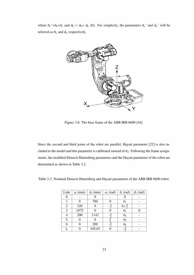
Figure 3.6 The base frame of the ABB IRB 6600 [44]. . . . . . . . . . . . . . . . . . 23

Figure 6.1 Experimental setup with Leica T-Mac mounted on the terminal frame of

the robot and Leica LTD500 laser tracker. . . . . . . . . . . . . . . . . . . . . . . 46

Figure 6.2 The technical drawings of the designed apparatus for the reference guide

holes and the 1.5” reflectors’ position on top of it. . . . . . . . . . . . . . . . . . 47

Figure 6.3 The top view of the four reference guides of the robot [44]. Dimensions

are in mm and radian. . . . . . . . . . . . . . . . . . . . . . . . . . . . . . . . . 47

Figure 6.4 The side-view of the reference guides of the robot [44]. Dimensions are in

mm. . . . . . . . . . . . . . . . . . . . . . . . . . . . . . . . . . . . . . . . . . 48

xiii

Figure 6.5 The images showing (a) reference guide, (b) the placing of the designed

apparatus to the reference guide and (c) the reflector placed on top of the apparatus

facing the measurement system sensor. . . . . . . . . . . . . . . . . . . . . . . . 48

Figure 6.6 The first set of 200 measurements according to the robot base coordinate

system. The measurement system is represented by the gray cylinder. The blue

lines show the orientation of the z-axes of the poses. . . . . . . . . . . . . . . . . 50

Figure 6.7 The second set of 325 measurements according to the robot base coordinate

system. The measurement system is represented by the gray cylinder. The blue

lines show the orientation of the z-axes of the poses. . . . . . . . . . . . . . . . . 51

Figure A.1 The Main window. . . . . . . . . . . . . . . . . . . . . . . . . . . . . . . 61

Figure A.2 The Kinematic Parameters window in simulation mode. . . . . . . . . . . 62

Figure A.3 The Kinematic Parameters window in application mode. . . . . . . . . . . 63

Figure A.4 The Measurement window in application mode. . . . . . . . . . . . . . . 64

Figure A.5 The Measurement window in simulation mode. . . . . . . . . . . . . . . . 65

Figure A.6 Generate / Load Measurements window. . . . . . . . . . . . . . . . . . . 66

Figure A.7 Generate / Load Measurement Noise window. . . . . . . . . . . . . . . . . 67

Figure A.8 The Optimization Settings window. . . . . . . . . . . . . . . . . . . . . . 68

Figure A.9 The results shown in the main window after pressing the Start Calibration

button. . . . . . . . . . . . . . . . . . . . . . . . . . . . . . . . . . . . . . . . . 69

Figure A.10The Pose Selection Interface. . . . . . . . . . . . . . . . . . . . . . . . . 70

xiv

CHAPTER 1

INTRODUCTION

Following the first installed industrial robot developed by Devol and Engelberger in 1961, the

use of industrial robots rapidly increased and they quickly became an indispensable part of

the manufacturing especially in the automotive industry. Today, they are used in a wide range

of applications and are capable of performing the difficult tasks they are programmed for.

The most common method of robot programming is performed on the factory floor by man-

ually teaching the robot the required poses of the task. While this method is tedious and

even hazardous in some cases, it benefits from the robot’s ability to successfully repeat a

previous instruction, a known quality of the industrial robots. On the other hand, emerging

programming methods make it possible to create robot tasks in a virtual environment without

interrupting the production cycle. While these new methods are proved to be less tiresome

and more efficient, they require the robot to be able to move to an instructed pose accurately.

This requirement put the robot’s accuracy into the spotlight.

The call for improving the accuracy of a robot without a redesign gave rise to the robot

calibration techniques. Robot calibration is being studied extensively for the last twenty-

five years, during which time, several studies have been conducted for better understanding

the error sources on robots and different methods have been proposed accordingly. However,

in an industrial point of view, a robot calibration method should not only be effective but also

should be efficient in terms of the time, effort and cost to be invested.

In this study, a rapid and an effective approach to the industrial robot calibration is sought.

According to this, the previous studies on the subject have been reviewed. A computer code

featuring a graphical user interface is developed to be used for both the simulations and the

calibration experiments. A novel and highly accurate measurement system is used to evaluate

1

the success of the calibration using additional measurements. Furthermore, an optimal pose

selection algorithm is used to obtain the poses amongst the gathered measurements in terms

of suppressing the measurement noise.

The pose error of a typical industrial robot and the part associated with the geometric pa-

rameters are inspected. Moreover, the effects of the measurement noise and the quality of

the measurements on the improvement of the accuracy of an industrial robot as a result of the

kinematic calibration are evaluated by simulations. The inverse geometric model is developed

to apply the error correction methods.

According to the results of the research and by using the selected methods, the necessary

computer tools along with graphical user interfaces are created which enable a progressive

kinematic calibration that can be used on a range of industrial robots on the factory environ-

ment. These developed computer tools are further tested on calibration experiments which

are proved to be efficient.

1.1 Objectives

The main objectives are:

• To investigate the robot calibration methods for their efficiency and to determine an

approach to be taken to calibrate industrial robots.

• To code the mathematical routines and to design graphical user interfaces to be used

during the simulations and the robot calibration procedure.

• To simulate the robot calibration using the designed tools and the generated measure-

ments with normally distributed noise.

• To perform robot calibration experiments and to evaluate the errors associated with the

nominal robot model.

• To evaluate the accuracy improvement of the robot as a result of the calibration using

the selected measurements.

2

1.2 Outline of the Thesis

Chapter 2 presents background information on robot calibration and reviews the related works

on the subject by presenting the approach and the techniques used on each step of the robot

calibration. The modeling methods used in the study and their implementation on the robot

under study are presented is Chapter 3. The details of the parameter identification and the

pose selection method are discussed in Chapter 4. The details of the simulations and their

results are presented at Chapter 5. The experiment on an industrial robot and its results are

presented in Chapter 6. The reached conclusions and the future work are discussed in Chapter

7.

3

CHAPTER 2

REVIEW OF ROBOT CALIBRATION METHODS

This chapter reviews the existing methods of robot calibration. The related information on the

subject like robot programming, performance evaluation and sources of error are given. The

previous works on the literature is also presented.

2.1 Robot Error Sources and Performance Evaluation

The performance requirements for industrial robots differ by the task they perform. The two

most frequently used performance criteria and their effect on different programming tech-

niques are discussed in the next sections.

2.1.1 Accuracy and Repeatability

The accuracy and the repeatability of an industrial robot are largely used to evaluate its perfor-

mance of reaching a desired pose. Repeatability is defined as the ability of the robot to reach

the same taught position while accuracy is defined as the ability of the robot to precisely reach

a programmed position [1]. Figure 2.1 shows the difference between the effect of accuracy

and repeatability on the final position of the robot’s end effector.

Many factors credited to affect the overall robot accuracy including but not limited to devia-

tions from nominal geometric parameters, joint offsets, link and joint compliance, gear trains,

gear backlash, gear runout and thermal factors [2, 3, 4, 5, 6]. The errors in geometric pa-

rameters are mainly due to the tolerances in manufacturing and the assembly of the robots’

parts. The flexibility of robot joints and the link deflection under self-gravity and load are

4

Figure 2.1: The effect of accuracy and repeatability [4].

attributed to compliance errors while thermal distortion and expansions of robot components

are attributed to thermal errors [7].

The robot pose errors are more generally divided into geometric and non-geometric errors

[2]. Geometric errors are caused by factors like joint offsets and deviations from the nominal

geometric parameters. Non-geometric errors are caused by other factors like joint and link

compliance, friction and clearance.

2.1.2 Programming

There are two common methods to program an industrial robot: online programming and

offline programming. The online programming of industrial robots involves teaching the robot

a sequence of poses manually, usually using a teach pendant, which all together compose a

specific task. Another method is to design the task using separate software and then load it to

the robot’s controller, which is known as offline programming. The visual robot simulation

programs and the production stops due to the time it takes to program each robot online make

5

Figure 2.2: Factors effecting the robot accuracy and repeatability. [4]

the latter method a better alternative. While the former method depends very much on the

repeatability, a characteristic that is known to be adequately high on today’s industrial robots,

the latter relies more on the accuracy of the industrial robots [3, 8]. In other words, for offline

programming methods to be applicable, the robot model that is used offline must accurately

describe the actual robot.

2.2 Robot Calibration

Robot calibration is a process that improves the accuracy of a robot by identifying a more ac-

curate functional relationship between the nominal and the actual robot [5]. The aim of robot

calibration is to improve the accuracy to reach the repeatability of the robot by modifications

through software.

Bernhardt and Albright classified the robot calibration into two types [9]: static and dynamic

calibration (Figure 2.3). Static calibration aims to identify the parameters that affect the static

positioning characteristics of the robot like link lengths, joint offsets, gear runout, gear back-

lash, actuator and link elasticity and coupling factor. Dynamic calibration, on the other hand,

deals with the identification of parameters that effect motion characteristics of the manipulator

like friction and the mass and the stiffness of the links and the actuators.

A more general classification is made by Roth, Mooring and Ravani where they divided the

robot calibration into three levels [5]: Level 1 is a joint level calibration which determines the

6

joint offset errors. Level 2 is an entire robot kinematic model calibration which determines

the basic kinematic geometry of the robot and the joint angle relationships. Finally, Level 3

is a non-kinematic calibration which determines the dynamic model of the robot.

Figure 2.3: Static and dynamic calibration classification of Bernhardt and Albright. [9]

In general, robot calibration is divided into four steps [5]:

• Modeling

• Measurements

• Identification

• Verification and Correction

2.2.1 Modeling

The first step of robot calibration is to establish a model that accurately maps the joint values

to the end-effector pose. Everett and later Schroer identified the three requirements for this

model to be used on the parameter identification stage as minimality, completeness and model

continuity or proportionality [10, 11, 12].

Minimality refers to the use of minimal number of parameters by the kinematic model. Com-

pleteness is the ability of the model to map joint values into end-effector positions for all

7

arbitrary manipulators. Model continuity or proportionality requires small changes in the

robot geometry to result small changes on the model parameters.

In an ideal case, this model accounts for all the factors that affect the robot pose errors. How-

ever, Mooring and Padavala argued that the effort associated with the more complex model is

not justified if it improves just a small amount of the resulting robot accuracy [13]. Further-

more, a good number of studies show that the geometric factors have much greater influence

on robot pose accuracy [3, 4, 7, 8, 13, 14, 15, 16].

The first study to include the non-geometric parameters to the calibration model is by Whitney

et al. which they used a model with geometric parameters as well as non geometric parameters

like joint compliance, backlash and gear transmission errors and calibrated a PUMA 560

robot using this model. Veitschegger and Wu calibrated a PUMA 560 robot by using position

measurements to identify the geometric parameters and showed that the positioning errors are

greatly reduced after the calibration [17]. Judd and Kasinski found out on their study with

two AID-900 robots that the joint angle offsets were accountable for nearly 90% of the total

rms error, deviations from nominal link parameters were accountable for a futher 5% and

gearing errors were only accountable for 1% of the total rms error [3]. Mooring and Padavela

calibrated a PUMA 560 robot using four different models with increasing complexity [13].

They reduced the initial mean positioning error of five poses from 30.04 mm to 0.47 mm

with a model consisting geometric parameters and joint offsets and to a further 0.42 mm

by adding compliance to this model. Caenen and Angue improved the mean accuracy of a

TH8 robot from 2.82 mm to 0.69 mm by only identifying the geometric parameters and to

a further 0.58 mm by identifying the non-geometric parameters associated with compliance

[15]. On their studies with Puma 760, Chen and Chao reduced the mean error distance of

5.9 mm to about 1 mm using geometric parameters and to an additional 0.28 mm by adding

non-geometric parameters to characterize the twist angles in the second and the third joints

and the backlash in third joint due to the gravitational effects [16]. Bernhardt showed the

effect of identifying additional parameter classes on the positioning errors of a typical spot

welding robot [14] (Figure 2.4). Gong et al. reduced the mean residual error of 30 positions

from 1.059 mm to 0.126 mm by identifying only the geometric parameters and to a further

0.088 mm after calibrating for compliance errors of the second and the third joints [7]. After

calibrating for these geometric and non-geometric errors, they also established and applied

empirical thermal error models to estimate thermal errors by monitoring the temperature field

8

at different operating conditions [7]. Jang et al. calibrated a DR06 robot for the geometric

errors in addition to the non-geometric joint angle deformations resulting from a payload by

dividing the robot workspace into several local regions and interpolating the identified errors

of each local region to obtain continuous functions of joint angles in the workspace [18]. More

recently, Gatla et al. calibrated a Staubli RX-130 robot by using only geometric parameters

which improved the robot’s mean deviation of aiming a laser at a fixed point from 5.64 mm

to 1.05 mm [8]. Lightcap, Hamner, Schmitz and Banks employed a two level optimization

algorithm to identify the geometric and flexibility parameters of a PA10-6CE robot using

measurements from a CMM where they reduced the positioning errors by 50 - 80% [19].

Figure 2.4: Reduction of positioning error 4TCP when identifying additional parameterclasses from none to full model [14].

Due to the results of these studies showing higher improvements in accuracy by just identify-

ing the geometric parameters and also the complexity of adding the non-geometric parameters

to the model, non-geometric factors are mainly discarded or neglected on the literature. The

main idea behind it is, -baring the errors caused by non-geometric factors- robot accuracy can

be greatly improved by identifying the geometric parameters of the robot. Moreover, since

most robot controllers use geometric parameters on their model, it is easier to correct these

parameters to improve the robot accuracy. This approach of identifying only the geometric

9

parameters is identical to the Level 2 calibration of Roth, Mooring and Ravani and it is still

largely used.

Figure 2.5: Denavit - Hartenberg parameters. [20]

The most widely used method of kinematic modeling is proposed by Denavit and Hartenberg

where homogenous transformation matrices are used to represent the relationship between

two consecutive link coordinate frames using four parameters [21] (Figure 2.5). These trans-

formation matrices are then multiplied to create a transformation between the base and the

end-effector coordinate systems. However, it has been shown by Hayati and Mirmirani that

when two consecutive joint axes are parallel or nearly parallel, Denavit - Hartenberg model

violates the model continuity or proportionality property since small changes in the robot ge-

ometry does not result small changes on the model parameters [22]. To overcome this, they

introduced an alternative parameterization to be used in case of parallel or nearly parallel

adjacent joint axes.

Alternative modeling techniques are also employed in robot calibration. Robertson and Du-

mont used genetic programming to obtain physical models by using mathematical operators

that evolved to the equations based on the measurements taken from the robot [23]. Dolinsky

et al. also used genetic programming to obtain evolved symbolic expressions of joint cor-

10

rection models for the first three joints of a PUMA 761 robot [24]. They reduced the mean

positioning error of the robot with this method from 1.85 mm to 0.77 mm.

It should also be noted that all of the studies discussed so far employ parametric models and

thus can be considered model-based approaches. There are also non-parametric or modeless

methods where the errors are approximated by using the measured data. An example to this

is the method proposed by Wang and Bai which uses a neural network algorithm to estimate

the positioning errors from the measured errors of the grids on a calibration board [25].

2.2.2 Measurements

The second step of robot calibration is obtaining the required data from the robot under study.

This data should be suitable to the model, in a sense, to relate the input of the established

model to the output [5].

Measurement systems used in the robot calibration have great importance in terms of iden-

tifying the model parameters and evaluating the robot performance. They should meet the

requirements of the calibration process in terms of accuracy and effectiveness. The measure-

ment systems used in the previous robot calibration studies include laser trackers [7, 26], op-

tical [8], photogrammetric [8, 18, 25, 27] and mechanical [24] systems, coordinate measuring

machines [13, 19] and theodolites [2, 16].

Hidalgo and Brunn showed that these measurement systems differ from each other not only by

their techniques but also by their characteristics like cost, sampling rate, set-up time, nominal

accuracy and repeatability [28]. They also showed that high cost systems do not necessarily

have higher accuracy, repeatability or resolution. Clearly, the most important properties are

accuracy and repeatability, but an ideal measurement system should also cost less and require

minimum amount of time to set-up. While most of the previous studies use optical and pho-

togrammetric systems, laser tracking systems are more frequently used in the industry for

their higher accuracy than their low-cost counterparts.

It should be noted that not all robot calibration methods require external measurement sys-

tems. Khalil et al. compared different geometric parameter calibration methods that use an

external measurement device or the joint encoder readings alone to identify the geometric

parameters [29]. The latter methods are considered as self-calibration methods on their study

11

which use specific constraints like the terminal link being on the same pose (or position) or

on the same plane for the chosen configurations.

2.2.3 Identification

The third step is to identify the parameters of the model using the gathered data. The most

common methods used in this stage are formulated as regression problems to determine the

parameters that minimize the error between the model and the measured data. Gauss-Newton

algorithm is used for nonlinear models for it quickly converges provided that the initial esti-

mates are close enough to the solution [30, 31]. This algorithm uses linear Taylor expansion

of the nonlinear model and then employs ordinary least squares iteratively.

However, Gauss-Newton algorithm is known to perform poorly in case of singular or ill-

conditioned matrices due to unidentifiable parameters, insufficient measurements and/or poor

scaling issues [30, 31]. Levenberg - Marquardt algorithm [32, 33], a modified version of the

Gauss-Newton algorithm, is a more robust choice in these cases.

Search algorithms can also be used on this stage but they are unavoidably slower. An example

to this is the study by Liu et.al where they used genetic algorithm in their simulations to

identify the geometric parameters of a PUMA 560 robot [34].

A lot of research on this step focuses on optimally selecting the measurement configurations

to improve the performance of the identification. This is stated as the problem of determining

a set of reachable robot measurement configurations that minimizes the effect of measurement

noise on the identification of robot kinematic parameters [35]. These measurements are se-

lected by using an observability index based on the identification Jacobian matrix. Driels and

Pathre proposed to use the condition number of the identification Jacobian [36] while Borm

and Menq proposed the geometric mean of all the singular values of the identification Jaco-

bian as the observability index [37]. Nahvi and Hollerbach proposed the minimum singular

value and also the square of smallest non-zero singular value divided by the largest singular

value of the identification Jacobian as observability indices [38, 39]. These observability in-

dices are reviewed by Sun and Hollerbach where they relate them to the alphabet optimalities

of the experimental design literature [39].

The methods used in finding the optimal measurements using the observability index also dif-

12

fer. Zhuang et.al proposed the use of the simulated annealing and later genetic algorithm on

selecting the optimum measurements arguing that gradient-based methods frequently trapped

into local minima [35, 40]. Sun and Hollerbach proposed a method called active robot cali-

bration algorithm based on DETMAX algorithm of Mitchell [41] but using determinant-based

updating observability index instead of an eigenvalue-based one [42]. Watanabe et al. pro-

posed an automatic calibration method that determines the poses to be measured based on

their condition number [27]. It should also be noted that Khalil and Besnard pointed out that

randomly selected measurements generally have sufficient condition number [29].

2.2.4 Verification and Correction

The final step of robot calibration is correcting the errors of the robot. The simplest way to do

this is by updating the identified parameter values inside the robot controller. However, most

robot controllers employ only the geometric parameters on their model. Furthermore, not all

robot controllers allow the nominal model parameters to be changed. Another method is to

change the robot program by updating the robot targets of the task. This requires the inverse

model of the robot to generate so-called fake targets. A final way is using an external unit to

correct the errors real time.

It is also a good practice to validate the accuracy of the identification prior to the correction

procedure. Since the identification algorithms use the supplied measurement data for esti-

mating the model parameters, additional measurements should be obtained from the robot to

verify these estimated parameters. This will also help to have a basic idea on the pose errors

before and after the calibration.

13

CHAPTER 3

KINEMATIC MODELING

This chapter presents the information on kinematic modeling of the IRB 6600 robot used

during the study. The mathematical background on the kinematic modeling and the modeling

of the robot under study are discussed in detail.

3.1 Mathematical Background

This section presents the representation of position and orientation, homogenous transforma-

tion and the geometric representation of serial-link robots, specifically method of Denavit and

Hartenberg. The sources used during this chapter are [6, 31, 43].

3.1.1 Representation of Position and Orientation

3.1.1.1 Position

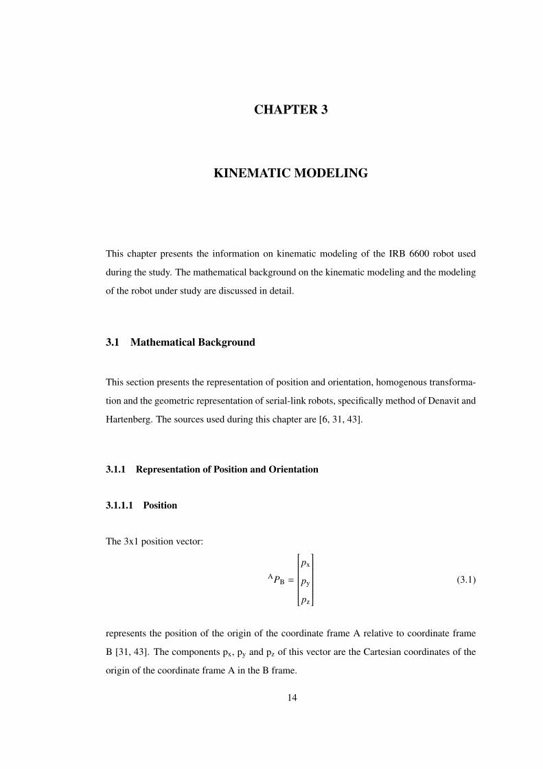
The 3x1 position vector:

APB =

px

py

pz

(3.1)

represents the position of the origin of the coordinate frame A relative to coordinate frame

B [31, 43]. The components px, py and pz of this vector are the Cartesian coordinates of the

origin of the coordinate frame A in the B frame.

14

3.1.1.2 Orientation

Let the unit vectors giving the principal directions of coordinate system B denoted as xB, yB,

zB. They can be written in terms of the coordinate system A as A xB, AyB, AzB. These three

unit vectors can be stacked on the columns of a 3x3 matrix:

ARB =

A xB

AyB

AzB

=

xB.xA yB.xA zB.xA

xB.yA yB.yA zB.yA

xB.zA yB.zA zB.zA

(3.2)

which is called the rotation matrix. The rotation of the frame A through an angle θ about the

xB axis is:

Rx(θ) =

1 0 0

0 cosθ −sinθ

0 sinθ cosθ

(3.3)

about the yB axis is:

Ry(θ) =

cosθ 0 sinθ

0 1 0

−sinθ 0 cosθ

(3.4)

and about the zB axis is:

Rz(θ) =

cosθ −sinθ 0

sinθ cosθ 0

0 0 1

(3.5)

3.1.2 Homogenous Transformation

Homogenous transformation combines the position and the orientation.

BTA =

BRABPA

0 1

(3.6)

The homogeneous transformation of a translation along an axis is denoted Trans. According

to this, the translation of l along the x axis can be written as:

Trans(x, θ) =

0 0 0 l

0 0 0 0

0 0 0 0

0 0 0 1

(3.7)

15

The homogeneous transformation of a rotation about an axis is denoted by Rot. According to

this, the rotation through an angle θ about the x axis can be written as:

Rot(x, θ) =

1 0 0 0

0 cosθ −sinθ 0

0 sinθ cosθ 0

0 0 0 1

(3.8)

3.1.3 Geometric Representation

Denavit and Hartenberg introduced a widely adopted convention for assigning frames to the

links of the robot [21]. A modified version of this convention by Khalil and Dombre is used

throughout this research [6]. This convention has an advantage of using the same subscript

for the parameters defining a transformation between two consecutive frames while it has a

drawback of denoting link lengths with a parameter having the same index of the consecutive

link.

The two main assumptions are: the links are perfectly rigid and the joints are ideal in a sense

that there is neither backlash nor elasticity [6]. A serial robot is composed of a sequence of

n-1 links and n joints where link 0 is the base of the robot and link n is the terminal link [6].

Joint i connects the link i to the link i-1 and its variable is denoted by θi [6]. A frame Ri is

attached to each link i with [6]:

• The zi axis is located along the axis of joint i.

• The xi axis is located along the common normal between the zi and zi+1 axis. If zi and

zi+1 axes are parallel or collinear, the choice of xi+1 is not unique. The intersection of

xi axis and zi axes defines the origin Oi. If the joint axes intersect, the origin is at the

point of intersection of the joint axes.

• The yi axis is located using the right-hand rule to form (xi,yi,zi) coordinate system.

The transformation matrix from frame Ri-1 to frame Ri is expressed using the following four

geometric parameters (Figure 3.1) [6]:

• Link twist: αi is the angle between zi-1 and zi about xi-1

16

Figure 3.1: The parameters αi, ai, θi and di [31].

• Link length: ai is the distance between zi-1 and zi along xi-1

• Joint angle: θi is the angle between xi-1 and xi about zi

• Link offset: di is the distance between xi-1 and xi along zi

And the transformation matrix defining the frame Ri relative to the frame Ri-1 is:

i-1Ti = Rot(x, αi)Trans(x, ai)Rot(z, θi)Trans(z, di)

=

cosθi −sinθi 0 ai

cosαisinθi cosαicosθi −sinαi −disinαi

sinαisinθi sinαicosθi cosαi dicosαi

0 0 0 1

(3.9)

As it is mentioned in the previous chapter, Denavit - Hartenberg representation faces a prob-

lem when two joint axes are parallel. When two consecutive joint axes i-1 and i are parallel,

the xi-1 axis is chosen arbitrarily along one of the common normals between them. If zi or zi-1

gets slightly misaligned, the common normal becomes uniquely defined and a big variation in

the parameter di-1 might occur [5, 6]. To overcome this problem, Hayati introduced a new pa-

rameter βi representing a rotation around the yi-1 axis [22]. Thus, the general transformation

matrix between two frames with consecutive parallel joints becomes [6] (Figure 3.2):

17

Figure 3.2: The additional parameter βi for consecutive parallel joints. [31].

i-1Ti = Rot(y, βi)Rot(x, αi)Trans(x, ai)Rot(z, θi)Trans(z, di) (3.10)

=

cβicθi + sαisβisθi sαisβicθi − cβisθi cαisβi aicβi + dicαisβi

cαisθi cαicθi −sαi −disαi

cβisαisθi − sβicθi sβisθi + cβisαicθi cαicβi dicαicβi − aisβi

0 0 0 1

where cγi stands for cosγi and sγi stands for sinγi. In such cases, the parameter βi is identified

instead of di.

3.1.4 Forward Kinematics

The forward kinematics problem for a serial-chain manipulator is defined as finding the pose

(position and orientation) of the end-effector relative to the base given the values of the joint

variables and the geometric link parameters [31]. It can be solved by calculating the transfor-

mation between the frames fixed in the end-effector and in the base [31]. This transformation

can be obtained by simply concatenating the transformations between the fixed frames of the

adjacent links [31]:

0Tn =0 T11T2 ...

n-2Tn-1n-1Tn (3.11)

18

3.1.5 Inverse Kinematics

The inverse kinematics problem for a serial-chain manipulator is defined as finding the values

of the joint variables given the pose of the end-effector relative to the base and the geometric

link parameters [31].

This problem can be solved algebraically or geometrically to obtain a closed-form solutions

or using numerical methods. While closed-form solutions depend on the particular robot, they

are faster than numerical solutions [31]. These solutions use particular geometric features like

spherical wrist where three consecutive revolute joint axes intersect at a common point [31].

A closed-form solution of an industrial robot used in this study will be presented in the later

sections.

3.2 Kinematic Modeling of ABB IRB 6600

This section presents the modeling of ABB IRB 6600 industrial robot.

3.2.1 Robot Description

ABB IRB 6600 industrial robot is selected as the robot of interest in this study. The version of

the particular robot is 2.55 / 175. This version numbers represent that its maximum reach at

wrist center is 2.55 meters and have a maximum handling capacity of 175 kg while it weighs

1.7 tons [44].

The positioning accuracy of the robot is reported on the production specification as 0.02 - 0.09

mm and the positioning repeatability is reported to as 0.08 - 0.18 mm [44]. The positioning

accuracy of the calibrated robot is reported to be 97% within 1 mm with an average of 0.5

mm and a maximum value of 1.2 mm [44]. The joint axis resolution is reported as 0.001◦ -

0.005◦.

ABB IRB 6600 industrial robot has six joint axes as shown in Figure 3.3. The type and the

range of motion of these joint axes are shown in Table 3.1.

19

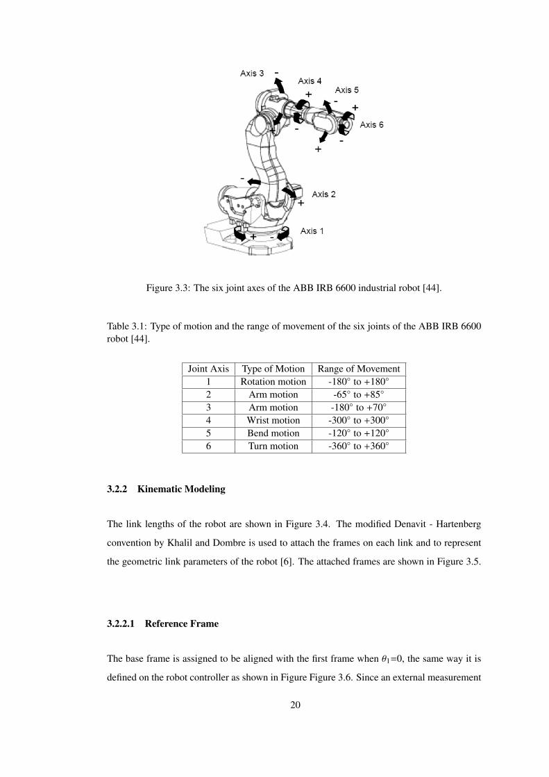
Figure 3.3: The six joint axes of the ABB IRB 6600 industrial robot [44].

Table 3.1: Type of motion and the range of movement of the six joints of the ABB IRB 6600robot [44].

Joint Axis Type of Motion Range of Movement1 Rotation motion -180◦ to +180◦

2 Arm motion -65◦ to +85◦

3 Arm motion -180◦ to +70◦

4 Wrist motion -300◦ to +300◦

5 Bend motion -120◦ to +120◦

6 Turn motion -360◦ to +360◦

3.2.2 Kinematic Modeling

The link lengths of the robot are shown in Figure 3.4. The modified Denavit - Hartenberg

convention by Khalil and Dombre is used to attach the frames on each link and to represent

the geometric link parameters of the robot [6]. The attached frames are shown in Figure 3.5.

3.2.2.1 Reference Frame

The base frame is assigned to be aligned with the first frame when θ1=0, the same way it is

defined on the robot controller as shown in Figure Figure 3.6. Since an external measurement

20

Figure 3.4: The description of the link lengths of the ABB IRB 6600 industrial robot [44].

system might obtain its measurements relative to a world reference frame, there is a need to

define this reference frame. Six parameters are required to locate the robot base frame relative

to a reference frame [6]:

RT0 = Rot(z, γR)Trans(z, bR)Rot(x, αR)Trans(x, aR)Rot(z, θR)Trans(z, dR) (3.12)

Then, the transformation matrix from the reference frame to the first link frame becomes:

RT1 = Rot(z, γR)Trans(z, bR)Rot(x, αR)Trans(x, aR)Rot(z, θR)Trans(z, dR) (3.13)

Rot(x, α1)Trans(x, a1)Rot(z, θ1)Trans(z, d1)

having α1 and a1 as zero, Eq. 3.14 can be written as:

RT1 = Rot(x, α0)Trans(x, a0)Rot(z, θ0)Trans(z, d0) (3.14)

Rot(x, α′

1)Trans(x, a′

1)Rot(z, θ′

1)Trans(z, d′

1)

where α0=0, a0=0, θ0=γR, d0=bR, α1’=αR, a1’= aR, θ1’=θ1+θR and d1’= d1+ dR [6]. For

simplicity, the parameters α1’, a1’, θ1’ and d1’ will be referred as α1, a1, θ1 and d1 respectively.

21

Figure 3.5: The attached frames for ABB IRB 6600 robot.

3.2.2.2 End-Effector Frame

The end-effector frame is assigned according to the mounting of T-Mac probe as shown in

Figure 6.1. Six parameters are required to locate the end-effector frame relative to last link

frame[6]:

6TL = Rot(z, γL)Trans(z, bL)Rot(x, αL)Trans(x, aL)Rot(z, θL)Trans(z, dL) (3.15)

Then, the transformation matrix from the fifth link frame to the end-effector frame becomes:

5TL = Rot(x, α6)Trans(x, a6)Rot(z, θ6)Trans(z, d6) (3.16)

Rot(z, γL)Trans(z, bL)Rot(x, αL)Trans(x, aL)Rot(z, θL)Trans(z, dL)

which can be written as:

5TL = Rot(x, α6)Trans(x, a6)Rot(z, θ′

6)Trans(z, d′

6) (3.17)

Rot(x, αL)Trans(x, aL)Rot(z, θL)Trans(z, dL)

22

where θL’=θ6+θL and dL’= d6+ dL [6]. For simplicity, the parameters θL’ and dL’ will be

referred as θL and dL respectively.

Figure 3.6: The base frame of the ABB IRB 6600 [44].

Since the second and third joints of the robot are parallel, Hayati parameter [22] is also in-

cluded to the model and this parameter is calibrated instead of d3. Following the frame assign-

ments, the modified Denavit-Hartenberg parameters and the Hayati parameter of the robot are

determined as shown in Table 3.2.

Table 3.2: Nominal Denavit-Hartenberg and Hayati parameters of the ABB IRB 6600 robot.

Link ai (mm) di (mm) αi (rad) θi (rad) βi (rad)0 - 0 - 0 -1 0 780 0 θ1 -2 320 0 -π2 θ2-π2 -3 1075 0 0 θ3 04 200 1142 -π2 θ4 -5 0 0 π

2 θ5 -6 0 200 -π2 θ6 -L 0 105.65 0 -π2 -

23

3.2.3 Forward Kinematics of ABB IRB 6600

Using Eq. 3.9 and 3.10 together with the Table 3.2, the transformation from the reference

frame to the end-effector frame of the robot can be calculated as:

RTL =R T00T1

1T22T3

3T44T5

5T66TL =

RRLRPL

0 1

(3.18)

where RRL is the 3x3 rotation matrix and RPL is the 3x1 position vector.

3.2.4 Inverse Kinematics of ABB IRB 6600

The closed-form solution of the inverse kinematic model is developed algebraically using the

derivations from Khalil and Dombre [6]. Only the non-zero link offsets and link lengths of the

Table 3.2 are taken into consideration along with the joint angles. It can be seen from Figure

3.5 that the fourth, fifth and sixth joint axes intersect forming a spherical wrist. The origins of

these frames are located at the same position making 0P6 = 0P4. This can be represented by:

px

py

pz

1

=0 T1

1T22T3

3T4

0

0

0

1

(3.19)

Multiplying Eq. 3.19 by 2T0 on both sides yields:

d1sinθ2 − a2cosθ2 − pzsinθ2 + pxcosθ1cosθ2 + pycosθ2sinθ1

d1cosθ2 − pzcosθ2 + a2sinθ2 − pxcosθ1sinθ2 − pysinθ1sinθ2

pycosθ1 − pxsinθ1

1

=

a3 + a4cosθ3 − d4sinθ3

d4cosθ3 + a4sinθ3

0

1

(3.20)

The three equations from Eq. 3.20 can be written as:

a4cosθ3 − d4sinθ3 = (d1 − pz)sinθ2 − (a2 − pxcosθ1 − pysinθ1)cosθ2 − a3 (3.21)

a4sinθ3 + d4cosθ3 = (d1 − pz)cosθ2 + (a2 − pxcosθ1 − pysinθ1)sinθ2 (3.22)

pycosθ1 − pxsinθ1 = 0 (3.23)

24

Eq. 3.23 can be used to solve for θ1 as [6]: θ1 = atan2(py, px)

θ′1 = θ1 + π

(3.24)

Eq. 3.22 and Eq. 3.21 can be written as:

W1cosθ3 + W2sinθ3 = Xsinθ2 + Ycosθ2 + Z1 (3.25)

W1sinθ3 −W2cosθ3 = Xcosθ2 − Y sinθ2 + Z2 (3.26)

where

W1 = a4

W2 = d4

X = d1 − pz

Y = a2 − pxcosθ1 − pysinθ1

Z1 = 0

Z2 = −a3

(3.27)

Squaring and adding the both sides of the Eq. 3.22 and 3.21 cancels the terms with θ3 and

yields an equation containing only θ2 in the form:

B1sinθ2 + B2cosθ2 = B3 (3.28)

where B1 = −2a3(d1 − pz)

B2 = 2a3(a2 − pxcosθ1 − pysinθ1)

B3 = a24 − (d1 − pz)2 − (a2 − pxcosθ1 − pysinθ1)2 − a2

3

(3.29)

From Eq. 3.28 [6]:

sinθ2 =B1B3 + εB2

2√

B21 + B2

2 − B23

B21 + B2

2

(3.30)

cosθ2 =B2B3 − εB1

2√

B21 + B2

2 − B23

B21 + B2

2

(3.31)

where ε=±1. Thus θ2 can be solved by using Eq. 3.30 and 3.31 as:

θ2 = atan2(sinθ2, cosθ2) (3.32)

Having found θ2, Eq. 3.22 and 3.21 reduce to the form:

X1sinθ3 + Y1cosθ3 = Q1 (3.33)

X2sinθ3 + Y2cosθ3 = Q2 (3.34)

25

where

X1 = Y2 = a4

X2 = −Y1 = −d4

Q1 = (d1 − pz)cosθ2 + (a2 − pxcosθ1 − pysinθ1)sinθ2

Q2 = (d1 − pz)sinθ2 − (a2 − pxcosθ1 − pysinθ1)cosθ2 − a3

(3.35)

Multiplying the Eq. 3.33 by Y2 and 3.34 by Y1 and adding both sides yields [6]:

sinθ3 =Q1Y2 − Q2Y1

X1Y2 − X2Y1(3.36)

Multiplying the Eq. 3.33 by X2 and 3.34 by X1 and adding both sides yields [6]:

cosθ3 =Q2X1 − Q1X2

X1Y2 − X2Y1(3.37)

Thus θ3 can be solved by using Eq. 3.36 and 3.37 as:


After finding θ1, θ2 and θ3, the rotation matrix of the third frame relative to the base frame,0R3, can be calculated. The rotation matrix of the final frame relative to the base frame is also

known and can be written as:

0R6 =

sx nx ax

sy ny ay

sz nz az

(3.39)

Thus the rotation matrix 3R6 can be calculated from:

3R6 =3 R00R6 =

fx gx hx

fy gy hy

fz gz hz

=3 R0

sx nx ax

sy ny ay

sz nz az

(3.40)

The same way, calculating 4R6:

4R6 =4 R33R6 =

fxcosθ4 − fzsinθ4 gxcosθ4 − gzsinθ4 hxcosθ4 − hzsinθ4

− fzcosθ4 − fxsinθ4 −gzcosθ4 − gxsinθ4 −hzcosθ4 − hxsinθ4

fy gy hy

=

cosθ5cosθ6 −cosθ5 − sinθ6 −sinθ5

sinθ6 cosθ6 0

cosθ6sinθ5 −sinθ5sinθ6 cosθ5

(3.41)

26

From the second rows and third columns of both sides of Eq. 3.41:

−hzcosθ4 − hxsinθ4 = 0 (3.42)

Eq. 3.42 can be used to solve for θ4 as [6]: θ4 = atan2(hz,−hx)

θ′4 = θ1 + π

(3.43)

Again from Eq. 3.41:

sinθ5 = −hxcosθ4 + hzsinθ4 (3.44)

cosθ5 = hy (3.45)

Solving Eq. 3.44 and 3.45 together for θ5 [6]:


And lastly from Eq. 3.41:

sinθ6 = − fzcosθ4 − fxsinθ4 (3.47)

cosθ6 = −gzcosθ4 − gxsinθ4 (3.48)

Solving Eq. 3.47 and 3.48 together for θ6 [6]:


27

CHAPTER 4

PARAMETER IDENTIFICATION

This chapter gives information about the pose selection and the parameter identification meth-

ods used during the study by their formulation, analysis and utilization to the model developed

on the previous chapter.

4.1 Parameter Identification Methods

Parameter identification methods used on the previous robot calibration studies are discussed

on the second chapter. Two of these algorithms based on least squares are presented in this

section.

4.1.1 Gauss-Newton Algorithm

The nonlinear kinematic model can be written as [30, 31]:

y = f(w, x) (4.1)

where w is the p x 1 parameter vector to be identified, y is the n x 1 output vector, f(w, x)

is n x 1 vector of functions and x is the k x 1 input vector. When there are m measurements

having n pose components, Eq. 4.1 can be written as [31, 30]:

yj = fj(w, xj) ( j = 1, . . . ,m) (4.2)

where fj(w, xj) = [ f j1(w, xj) . . . f j

n(w, xj)]T is the n x 1 vector of functions, yj = [yj1 . . . y

jn]T is

the n x 1 output vector and xj = [xj1 . . . xj

k]T is the k x 1 input vector for the jth measurement.

28

The least-square solution seeks the estimate w of the actual value of the parameter vector w

that minimizes the sum of squares of the error between the model and the measurements:

S (w) =

m∑j=1

‖ yj − f(w, xj) ‖2= rTr (4.3)

where r is the nm x 1 residual vector:

r =

y11 − f 1

1 (w, x1)

y12 − f 1

2 (w, x1)...

yjn − f j

n(w, xj)...

ymn-1 − f m

n-1(w, xm)

ymn − f m

n (w, xm)

(4.4)

Taking linear Taylor series approximation of fj(w, xj) about an initial estimate of the parameter

vector wa yields:

fj(w, xj) ≈ fj(wa, xj) +∂fj(w, xj)

∂w|w=wa (w − wa) (4.5)

Solving for the minimum of Eq. 4.3 with respect to w using Eq. 4.5 yields [30]:

(w − wa) = δa = (JaTJa)-1JaTr (4.6)

where

Ja =

∂f1(w,x1)

∂w |w=wa

...

∂fm(w,xm)∂w |w=wa

(4.7)

is the nm x p identification Jacobian matrix. Eq. 4.29 is called Gauss-Newton step [30]. Thus,

given an initial estimate wa, the next estimate can be calculated from:

wa+1 = wa + δa = wa + (JaTJa)-1JaTr (4.8)

which is repeated iteratively until the error is less than a tolerance value or a convergence is

obtained.

4.1.2 Levenberg - Marquardt Algorithm

Gauss-Newton algorithm is known for its fast convergence. However, a problem arise when

the matrix JTJ is not invertible for being singular or ill-conditioned. Levenberg and Marquardt

29

algorithm solves this problem by modifying the Gauss-Newton step as [30, 32, 33]:

δa = (JaTJa + µaDa)-1JaTr (4.9)

where Da is a diagonal matrix containing positive elements and µais a scalar. Da can be chosen

as identity matrix for simplicity or the diagonal elements of the matrix JaTJa are used. µa is

generally set as a low value and it is multiplied by a factor whenever Eq. 4.3 is not reduced

as a result of the iteration.

4.2 Parameter Identification of ABB IRB 6600

In this section, the details of the employment of the parameter identification procedure for

ABB IRB 6600 robot are presented.

4.2.1 Formulation

For the utilized robot calibration scheme and according to Eq 4.2 and 4.8, output vector con-

sists of the pose measurements, input vector consists of the joint variables and the parameters

not included on the identification and the vector of functions are the nonlinear equations ob-

tained from Eq 3.18.

The parameter vector is a 30 x 1 vector consisting of all 30 parameters of Table 3.2:

w = [α1 . . . αL a1 . . . aL d0 . . . d2 d4 . . . dL θ0 . . . θL β3]T (4.10)

with the assumption of all parameters being identifiable. The identifiability of the parameters

will be investigated on the next section.

Let m pose measurements be taken from the robot’s end-effector frame having three position

and three orientation components. The joint configurations of the robot corresponding to the

jth measurement can be expressed as :

θj = [θj1,meas θ

j2,meas θ

j3,meas θ

j4,meas θ

j5,meas θ

j6,meas]

T ( j = 1, . . . ,m) (4.11)

and the jth measurement can be expressed as:

yj = [Pjx,meas Pj

y,meas Pjz,meas γ

jx,meas γ

jy,meas γ

jz,meas]

T ( j = 1, . . . ,m) (4.12)

30

where the superscript ‘meas’ denotes that these are obtained from measurements. Same way,

the pose of the end-effector for the jth measurement configuration can be calculated using Eq.

3.18 and 4.11 together with the parameters from Table 3.2 as:

RTL,calc =

RRj

L,calc

Pjx,calc

Pjy,calc

Pjz,calc

0 1

( j = 1, . . . ,m) (4.13)

where the superscript ‘calc’ denotes that these are obtained from calculations. In order to form

the residue vector for the jth measurement configuration, the difference between the calculated

and the measured position and orientation of the end-effector is needed to be obtained:

rj =

∆Pj

∆Oj

( j = 1, . . . ,m) (4.14)

Since the measurement system represents the orientation using Z-Y-X Euler angles, the Euler

angles from the matrix RRcL,calc can be extracted. However, the calculation of the identification

Jacobian will be far too tedious using this approach. For this reason, the approach of Khalil

and Dombre is used to represent the orientation error by using rotation matrices. The rotation

matrix from the jth measured orientation can be calculated by:

RRjL,meas = Rot(z, γj

z,meas)Rot(y, γjy,meas)Rot(x, γj

x,meas) (4.15)

and the orientation error can be expressed as [6]:

∆Oj = ujαj (4.16)

where

RRjL,meas = Rot(uj, αj)RRj

L,calc (4.17)

31

Thus, the 6m x 1 residue vector becomes:

r =

r1

r2

...

rm

=

∆P1

∆O1

...

∆Pm

∆Om

=

P1x,meas − P1

x,calc

P1y,meas − P1

y,calc

P1z,meas − P1

z,calc

u11α

1

u12α

1

u13α

1

...

Pmx,meas − Pm

x,calc

Pmy,meas − Pm

y,calc

Pmz,meas − Pm

z,calc

um1 α

m

um2 α

m

um3 α

m

(4.18)

For pose measurements, the identification Jacobian has one row for each of the six pose

element of each of the m measurements and one column for each of the p parameters making

it a 6m x p matrix. The individual Jacobian matrices of the parameters can be calculated by

[6, 31]:

Jjαi =

Rxji-1 ×

Rdji-1,L

Rxji-1

(4.19)

Jjai =

Rxji-1

0

(4.20)

Jjdi

=

Rzji

0

(4.21)

Jjθi

=

Rzji ×

Rdji,L

Rzji

(4.22)

32

Jjβi

=

Ryji-1 ×

Rdji-1,L

Ryji-1

( j = 1, . . . ,m) (4.23)

for ( j = 1, . . . ,m) whereRdj

i,L =R Rji

iPjL (4.24)

is the vector connecting the origin of the coordinate frame i to the origin of the coordinate

frame L [6, 31]. Concatenating all individual Jacobian matrices for all p parameters for the jth

measurement yields 6 x p matrix:

Jj = [Jjα1 . . . J

jαL Jj

a1 . . . JjaL Jj

d0. . . Jj

d2Jj

d4. . . Jj

dLJjθ0. . . Jj

θLJjβ3

] (4.25)

and concatenating this matrix for all m measurements yields the 6m x p generalized Jacobian

matrix:

J =

J1

J2

...

Jm

(4.26)

4.2.2 Identifiability

It is known that some parameters of the model cannot be identified as a result of zero or

linearly dependent columns of the matrix J. If a column of the matrix J is zero, then the

parameter corresponding to that column has no effect on the output and thus cannot be iden-

tified. Furthermore, the rank of the matrix J equals to the number of parameters that can be

identified [6].

The parameters of the robot that are not identifiable can be obtained using the method pre-

sented by Khalil et.al [29]. According to this, the identifiable parameters of the robot are

determined using a QR decomposition of J as [29]:

J = Q

R

0(r-c)xc

(4.27)

where Q is an r x r orthogonal matrix, R is a c x c upper triangular matrix and 0 is a (r-c) x c

zero matrix [29]. The non-identifiable parameters correspond to the absolute value elements

33

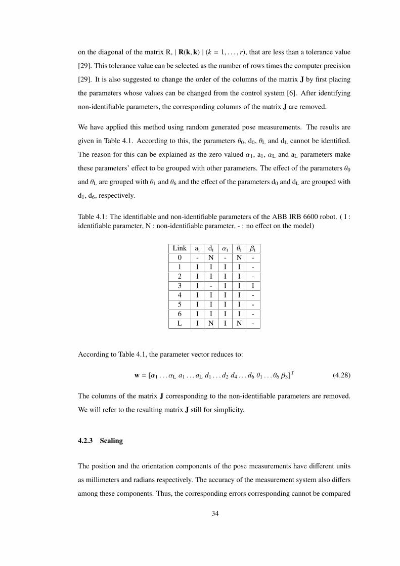
on the diagonal of the matrix R, | R(k,k) | (k = 1, . . . , r), that are less than a tolerance value

[29]. This tolerance value can be selected as the number of rows times the computer precision

[29]. It is also suggested to change the order of the columns of the matrix J by first placing

the parameters whose values can be changed from the control system [6]. After identifying

non-identifiable parameters, the corresponding columns of the matrix J are removed.

We have applied this method using random generated pose measurements. The results are

given in Table 4.1. According to this, the parameters θ0, d0, θL and dL cannot be identified.

The reason for this can be explained as the zero valued α1, a1, αL and aL parameters make

these parameters’ effect to be grouped with other parameters. The effect of the parameters θ0

and θL are grouped with θ1 and θ6 and the effect of the parameters d0 and dL are grouped with

d1, d6, respectively.

Table 4.1: The identifiable and non-identifiable parameters of the ABB IRB 6600 robot. ( I :identifiable parameter, N : non-identifiable parameter, - : no effect on the model)

Link ai di αi θi βi

0 - N - N -1 I I I I -2 I I I I -3 I - I I I4 I I I I -5 I I I I -6 I I I I -L I N I N -

According to Table 4.1, the parameter vector reduces to:

w = [α1 . . . αL a1 . . . aL d1 . . . d2 d4 . . . d6 θ1 . . . θ6 β3]T (4.28)

The columns of the matrix J corresponding to the non-identifiable parameters are removed.

We will refer to the resulting matrix J still for simplicity.

4.2.3 Scaling

The position and the orientation components of the pose measurements have different units

as millimeters and radians respectively. The accuracy of the measurement system also differs

among these components. Thus, the corresponding errors corresponding cannot be compared

34

directly. In order to overcome this problem, Eq. 4.29 can be scaled by an appropriate weight-

ing matrix W as [31]:

(w − wa) = δa = (JaTWJa)-1JaTWr (4.29)

The measurement system used to obtain pose measurements is capable of giving the standard

deviation values of the measured variables. Let the standard deviation of the kth pose com-

ponent of the jth measurement be σjk for (k = 1, . . . , 6) and ( j = 1, . . . ,m). These standard

deviation values can be used on the corresponding diagonal element of the weighting matrix

as [31]:

W =

( 1σ1

1)2 . . . . . . . . . . . . 0

0 ( 1σ1

2)2 . . . . . . . . . 0

.... . .

...

0 . . . . . . ( 1σ

jk

)2 . . . 0

.... . .

...

0 . . . . . . . . . . . . ( 1σm

6)2

k = 1, . . . , 6

j = 1, . . . ,m(4.30)

4.3 Pose Selection

The success of the parameter identification on finding accurate estimates of the parameters is

effected by the measurement noise, the number of measurements and the selection of mea-

surement configurations [36]. A common practice to suppress the measurement noise in order

to achieve better estimates of the parameters is to increase the number of measurements used

in the identification step. However, a better approach is to select the measurement configura-

tions which will yield good estimates.

The determination of a set of reachable robot measurement configurations that minimizes the

effect of the measurement noise on the identification of robot kinematic parameters is the

subject of the optimal pose selection algorithms [35]. These measurement configurations are

selected using an observability index based on the identification Jacobian matrix. Several ob-

servability indices are proposed to be used on robot calibration experiments which are related

to the alphabet optimalities of the experimental design literature by Sun and Hollerbach [39]:

• O1 is proposed by Borm and Menq [37]. It is the geometric mean of all the singular

35

values of the identification Jacobian:

O1 =(σ1σ2 · · ·σk)

1k

√k

(4.31)

• Driels and Pathre proposed the condition number of the identification Jacobian as the

observability index to be minimized [36]. Since all other observability indices are max-

imized, it is taken as the inverse of the condition number of the identification Jacobian

[38]:

O2 =σMin

σMax(4.32)

• O3 is proposed by Nahvi and Hollerbach [38]. It is the minimum singular value of the

identification Jacobian:

O3 = σMin (4.33)

• O4 is again proposed by Nahvi and Hollerbach [38]. It is the square of smallest non-

zero singular value divided by the largest singular value of the identification Jacobian:

O4 =σ2

Min

σMax(4.34)

In this study, we have selected O1 as the observability index for its scale invariant charac-

teristic that also corresponds to the D-optimal design of the experimental design literature

[39].

A search algorithm is used to obtain the measurements configurations that maximize the se-

lected observability index amongst a set of all possible measurement configurations. DET-

MAX, a popular algorithm proposed by Mitchell can be used to find the measurement configu-

rations that maximize the observability index [41]. The basic algorithm follows the procedure

below:

1. Start by choosing a set of m measurement configurations randomly from the possible

candidate measurement configurations.

2. Add a new measurement configuration to the current set amongst the candidate set that

makes the maximum increase in the observability index.

3. Remove the measurement configuration amongst the current set that makes the mini-

mum decrease in the observability index.

36

4. Repeat 2 and 3 until the observability index does not increase.

This procedure improves the observability index of a randomly selected set by exchanging

measurement configurations at each iteration. The original algorithm also performs a method

called excursion that adds or removes new measurement configurations to improve the cur-

rent set. A variation of the algorithm is proposed by Sun and Hollerbach which starts with a

randomly selected set size, improves the set using the exchanging step then adds new mea-

surement configurations until a predefined number is reached [42]. In this study, a variation

of the DETMAX is used which first calculates the observability index of the whole candidate

set and then removes the measurement configurations that makes the minimum decrease in

the observability index until a pre-defined number of measurements is reached. The algorithm

then uses this as the initial set and applies the DETMAX algorithm until observability index

does not increase. The algorithm then removes a pose within the selected set and searches the

candidate set for a better pose that increases the observability index. This algorithm follows

the procedure below:

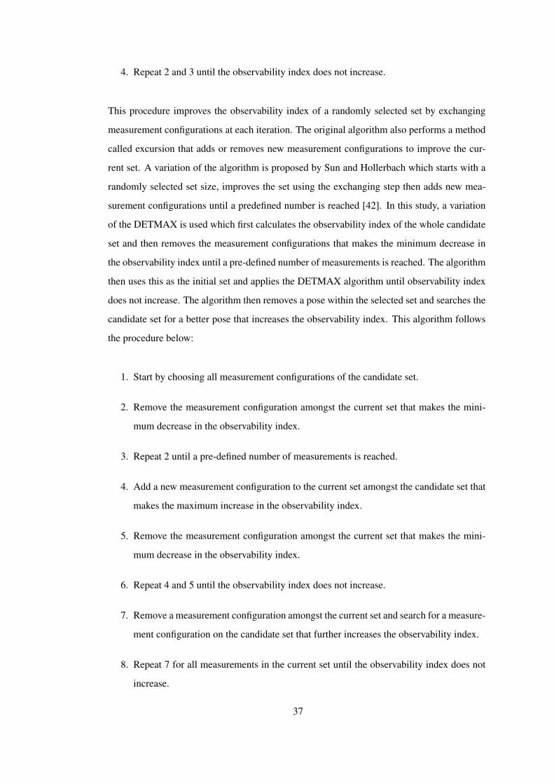
1. Start by choosing all measurement configurations of the candidate set.



3. Repeat 2 until a pre-defined number of measurements is reached.

4. Add a new measurement configuration to the current set amongst the candidate set that

makes the maximum increase in the observability index.



6. Repeat 4 and 5 until the observability index does not increase.

7. Remove a measurement configuration amongst the current set and search for a measure-

ment configuration on the candidate set that further increases the observability index.

8. Repeat 7 for all measurements in the current set until the observability index does not

increase.

37

The major advantage of the algorithm is starting with a selected initial set instead of a random

one. The concatenated identification Jacobian in Eq. 4.26 is calculated only once in the first

step. It should be noted that as the number of measurements in the candidate set increases,

the calculation of the identification Jacobian for all candidate measurements will require more

computer time. However, it takes less than three minutes in Matlab by using a PC with Intel

2.4 GHz processor and 3 GBs of RAM for a candidate set of 300 measurement configurations

and 24 model parameters which correspond to an 1800 x 24 matrix. This algorithm is used

during the simulations and the experiments. The designed graphical interface is shown in

Appendix A.

38

CHAPTER 5

SIMULATIONS

This chapter presents the details and the results of the simulations of the kinematic calibration

procedure that is performed by using the developed code and the designed user interface in

MATLAB.

5.1 Simulation Parameters

The model of ABB IRB 6600 robot previously developed in the Chapter 3 is used during

the simulations. The actual values of the parameters to be identified are generated by adding

pre-defined deviations to the nominal parameters of this robot given in Table 3.2. The devi-

ations from the nominal parameters are shown in Table 5.1. These deviations are selected to

characterize the identified deviations in previous calibration experiments.

Table 5.1: Selected deviations from the nominal Denavit - Hartenberg and Hayati parametersfor simulations.

Link ai (mm) di (mm) αi (mrad) θi (mrad) βi (mrad)0 - - - - -1 1.4 2.1 1.8 0.9 -2 -0.6 0.4 -0.7 -3.8 -3 0.4 - 1.2 1.7 -0.84 -2.8 2.5 1.9 2.9 -5 -0.9 -1.8 -1.6 -4.8 -6 0.7 0.9 1.4 3.9 -L -0.4 - 0.9 - -

39

5.2 Simulation Measurements

In order to obtain the measurement configurations to be used during the simulations, random

joint angle configurations are generated. These joint values are then used to solve the end-

effector pose using Eq 3.18. A sample measurement sensor is assigned to a selected location

to illustrate the conditions to be faced during the experiments. Each generated measurement

is checked inside the code to verify if:

• the joint angle values are inside the range of movement of the robot joints shown in

Table 3.1.

• the z-axis of the robot end-effector frame inclines towards the sample measurement

sensor by an angle of less than 30◦.

The need for the first condition is self evident while the second condition is commonly sought

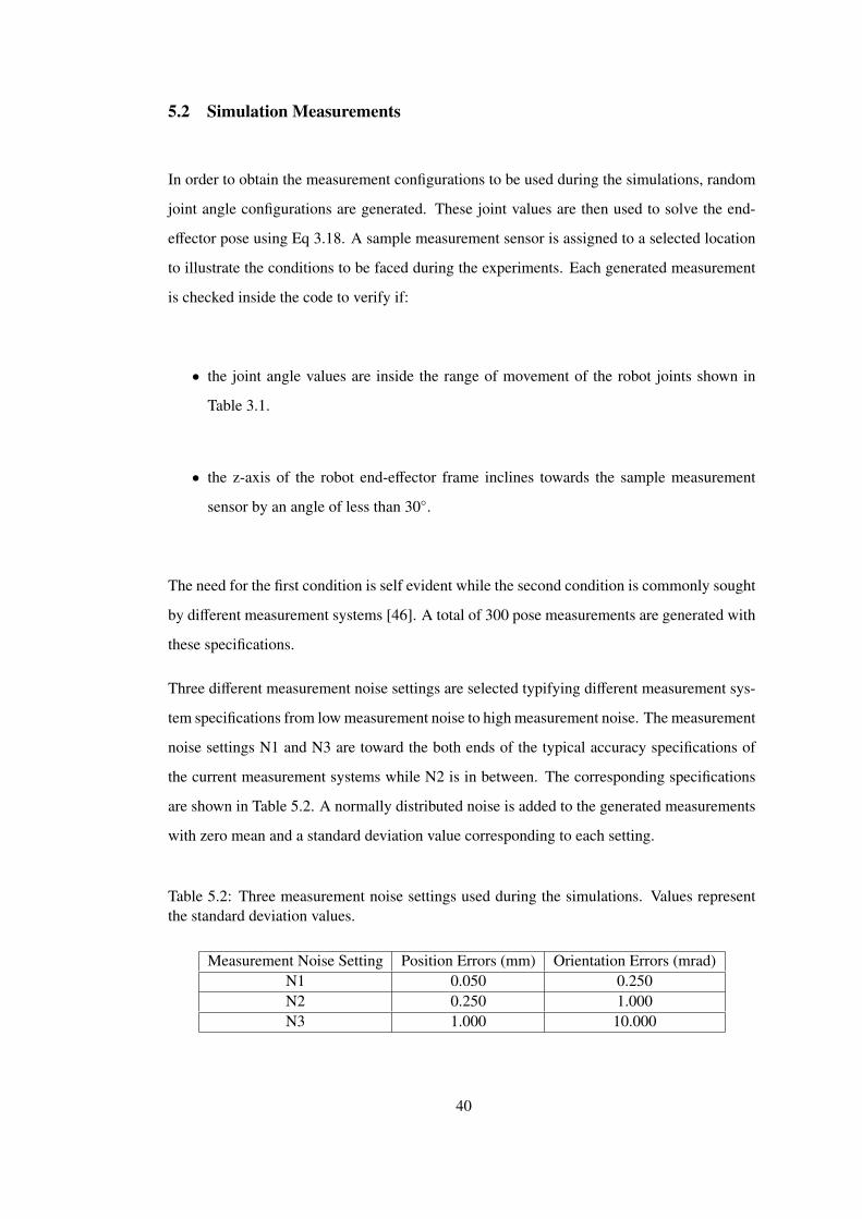
by different measurement systems [46]. A total of 300 pose measurements are generated with

these specifications.

Three different measurement noise settings are selected typifying different measurement sys-

tem specifications from low measurement noise to high measurement noise. The measurement

noise settings N1 and N3 are toward the both ends of the typical accuracy specifications of

the current measurement systems while N2 is in between. The corresponding specifications

are shown in Table 5.2. A normally distributed noise is added to the generated measurements

with zero mean and a standard deviation value corresponding to each setting.

Table 5.2: Three measurement noise settings used during the simulations. Values representthe standard deviation values.

Measurement Noise Setting Position Errors (mm) Orientation Errors (mrad)N1 0.050 0.250N2 0.250 1.000N3 1.000 10.000

40

5.3 Simulation Results

Amongst the generated 300 measurements, a set of 30 pose measurements are selected us-

ing the pose selection algorithm discussed in Section 4.3 with random deviations from the

nominal parameters. Additionally, 100 pose sets of 30 measurements are selected randomly.

Simulations are performed using the three different measurement noise settings.

Table 5.3: The estimation errors on the parameters after the identification with the selectedand 100 random measurement poses for N1 measurement noise settings.

ParameterSelected 100 Random Sets

Set Mean Std Dev Maximum Minimumα1 (mrad) 0.0016 0.0080 0.0058 0.0270 0.0002α2 (mrad) 0.0345 0.0170 0.0141 0.0558 0.0001α3 (mrad) 0.0142 0.0149 0.0110 0.0556 0.0003α4 (mrad) 0.0796 0.0526 0.0408 0.1913 0.0002α5 (mrad) 0.0338 0.0428 0.0347 0.1450 0.0004α6 (mrad) 0.0389 0.0612 0.0534 0.2737 0.0010α7 (mrad) 0.0410 0.0578 0.0456 0.2283 0.0002a1 (µm) 23.5508 15.6856 12.7318 66.9892 0.2029a2 (µm) 4.9088 13.6028 11.0028 60.1883 0.2190a3 (µm) 8.8517 16.9422 12.0693 51.0957 0.1696a4 (µm) 28.8407 57.7177 40.2227 205.2924 0.3722a5 (µm) 9.5533 8.2622 6.4702 34.5722 0.0267a6 (µm) 8.8604 25.7720 17.2785 74.027 0.0626a7 (µm) 2.3841 9.1991 7.6838 39.7336 0.1072d1 (µm) 0.7375 19.5358 14.1109 66.4082 0.2172d2 (µm) 111.0884 72.9885 55.9308 296.7127 0.3825d4 (µm) 2.4915 13.9625 11.4551 46.345 0.0665d5 (µm) 1.5375 22.3674 15.4093 81.2006 0.0169d6 (µm) 5.6842 15.4013 11.5797 45.8911 0.0813β3 (mrad) 0.0060 0.0231 0.0183 0.1049 0.0001θ1 (mrad) 0.0086 0.0118 0.0078 0.0338 0.0002θ2 (mrad) 0.0015 0.0118 0.0093 0.0517 0.0001θ3 (mrad) 0.0012 0.0467 0.0332 0.1757 0.0002θ4 (mrad) 0.0546 0.0526 0.0437 0.2076 0.0011θ5 (mrad) 0.0458 0.0807 0.0576 0.2131 0.0014θ6 (mrad) 0.0102 0.0584 0.0457 0.1854 0.0001

The algorithm is run until the change in the sum of errors did not exceed the defined tolerance

value or the algorithm reached the tenth iteration, whichever is satisfied first. It is seen that

the algorithm is typically converged at the third iteration during the simulations.

41

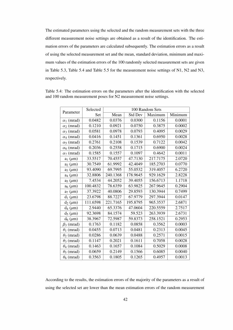
The estimated parameters using the selected and the random measurement sets with the three

different measurement noise settings are obtained as a result of the identification. The esti-

mation errors of the parameters are calculated subsequently. The estimation errors as a result

of using the selected measurement set and the mean, standard deviation, minimum and maxi-

mum values of the estimation errors of the 100 randomly selected measurement sets are given

in Table 5.3, Table 5.4 and Table 5.5 for the measurement noise settings of N1, N2 and N3,

respectively.




According to the results, the estimation errors of the majority of the parameters as a result of

using the selected set are lower than the mean estimation errors of the random measurement

42




sets. Only the estimation errors of a1, a5, d2, α2, α4 and θ4 in the selected measurement set

are greater than the mean estimation errors of the random measurement sets using the least

measurement noise setting N1. The same way, the estimation errors of a3, a6, d5, α1, α2, α5,

α7, β3 and θ6 using N2 measurement noise setting and the estimation errors of a7, d6 and α3

using N3 measurement noise setting in selected measurement set are greater than the mean

estimation errors of the random measurement sets. Only the estimation errors of α2 for the

N1 measurement noise setting and θ6 for the N2 measurement noise setting are greater than

the mean plus the standard deviation value of the estimation errors of random sets.

The expected effect of the measurement noise on the estimation errors of parameters can

43

also be seen on these tables, in that, as the measurement noise increases, the estimation errors

rapidly deteriorate. Especially, using the N3 measurement noise setting, most of the maximum

estimation errors of the random sets are greater than the initial errors of the parameters.

Table 5.6: The RMS errors of the end effector pose before and after identification with opti-mally selected measurement poses having three different measurement noise profile.

Pose Component Initial Error N1 N2 N3∆PX (mm) 1.367 0.010 0.048 0.158∆PY (mm) 1.238 0.011 0.043 0.175∆PZ (mm) 1.897 0.009 0.040 0.135∆γX (mrad) 4.233 0.044 0.356 0.991∆γY (mrad) 1.855 0.024 0.128 0.410∆γZ (mrad) 3.969 0.039 0.365 1.174

After the selected pose measurements are removed from the initial set of 300 generated pose

measurements, the remaining set is used to examine the pose errors of the robot end-effector

prior to and after the calibration. The results are shown in Table 5.6 for using the selected

pose measurements with different measurement noise specifications.

According to the results using the lowest measurement noise settings, the initial errors are

reduced for more than 98% for all pose components. For the highest measurement noise,

while the improvements on robot pose accuracy significantly dropped, the initial errors are

still reduced for more than 70% for all pose components. The worst effected pose components

from the measurement noise are the ones representing the orientation. On the other hand, the

positioning accuracy improvements from the initial errors are still higher than 85% despite this

high measurement noise setting. As an expected result, it can be seen that the improvements

on robot pose accuracy greatly decrease as the measurement noise further increases.

44

CHAPTER 6

EXPERIMENTS

This chapter presents the details and the results of the kinematic calibration experiments that

are performed by using the developed code and the designed user interface in MATLAB.

6.1 Experimental Setup

The experiments are performed on an ABB IRB 6600 industrial robot. The nominal Denavit-

Hartenberg and Hayati parameters of this robot are derived in the Chapter 3 which are given

in Table 3.2.

6.1.1 Measurement System

Leica LTD 500 Laser Tracker is used as the measurement system during the experiments. This

laser tracker system uses the absolute distance measurements together with the two angle

values from the encoder readings to obtain 3D measurements. In order to obtain full pose

measurements from the robot, a Leica T-Mac probe is used which is directly mounted on the

robot end-effector using an apparatus as shown in Figure 6.1. The accuracy specifications of

the Leica LTD500 laser tracker and the T-Mac probe are shown in Table 6.1.

In order to register the reference coordinate system to the measurement system, the reference

guides on the robot body are used. There are a total of four reference guides on the robot

and the center of the reference guides are on a circle with its center about on the base frame

origin and having a radius of 400 mm which can be seen in Figures 6.3. Concerning the rapid

45

Figure 6.1: Experimental setup with Leica T-Mac mounted on the terminal frame of the robotand Leica LTD500 laser tracker.

Table 6.1: Accuracy specifications of Leica LTD 500 laser tracker and Leica T-Mac probe[45, 46].

Leica LTD500 Absolute accuracy of a coordinate fornon-moving target (2σ value)

±10µm/m + 6 µm/m

Leica T-Mac Accuracy of rotation angles (Maxi-mum Permissible Error)

0.01◦

Leica T-Mac Positional accuracy (Maximum Per-missible Error)

±15µm + 6µm/m

measurements to be taken from these reference guides, an apparatus that can be mounted

inside the reference guide holes is designed according to the dimensions of the reference

guide holes shown in Figure 6.4. The apparatus is also designed so that 1.5’ reflectors can be

placed on top of it as seen on the Figure 6.2. The calculated positions of the center of these

reference guides are shown in Table 6.2. Figure 6.5 shows one of the reference guides, the

designed apparatus placed on it and the reflector placed on top of the apparatus.

46

Figure 6.2: The technical drawings of the designed apparatus for the reference guide holesand the 1.5” reflectors’ position on top of it.

Figure 6.3: The top view of the four reference guides of the robot [44]. Dimensions are inmm and radian.

47

Figure 6.4: The side-view of the reference guides of the robot [44]. Dimensions are in mm.

(a) (b) (c)

Figure 6.5: The images showing (a) reference guide, (b) the placing of the designed appa-ratus to the reference guide and (c) the reflector placed on top of the apparatus facing themeasurement system sensor.

48

Table 6.2: The position of the four reference guides.

Point X (mm) Y (mm) Z (mm)Pr1 282.8427 282.8427 110.5000Pr2 -282.8427 282.8427 110.5000Pr3 -282.8427 -282.8427 110.5000Pr4 282.8427 -282.8427 110.5000

6.1.2 Measurements

There were three limitations that are faced during the selection of the poses to be measured:

1. The first joint angle is bounded at 120◦ rose from the robot workcell conditions.

2. Leica LTD 500 Laser Tracker requires the z-axis of the T-Mac probe to be aligned with

the sensor by an angle of less than 45◦.

3. The laser beam from the Leica LTD 500 Laser Tracker reaching to the reflector on the

T-Mac should not be interrupted while the robot is moving from one pose measurement

configuration to the other.

The first and the second conditions are straightforward to check and satisfy while the third

condition requires the robot trajectory between the consecutive measured poses to also satisfy

the second condition.

In order to meet these conditions, paths to be followed by the robot end-effector are defined

in the joint space. The firs path is defined using 64 pose measurements and extended to 200

measurements by selecting additional poses on the path. The second path is defined using 84

pose measurements and extended to 325 by again selecting additional poses on the path. The

selected poses for the first and the second set of measurements are shown in Figure 6.6 and

6.7, respectively.

The measurements from the first set and the second set are taken two months apart, during

which time the robot is continued to be used and even some parts of the robot are replaced.

The only nominal parameter of the robot that is changed while the second set of measurements

were taken is the d7 resulting from the removal of the 5 mm washers that were between the

T-Mac probe and the robot end-effector. Thus, the nominal value of the d7 parameter is taken

49

as 106.5 mm for the first set of measurements while taken as 101.5 mm for the second set on

the parameter identification stage.

The measurements are taken by using a code written in Visual Basic together with the related

functions of emScon Software Development Kit (SDK) of Leica Laser Tracker. The Visual

Basic for Applications (VBA) inside Microsoft Excel 2007 is used for both creating a basic

GUI and for storing the associated measurement data on the worksheets. This proved to be

useful for taking the measurements rapidly and loading these measurements to the designed

kinematic calibration GUI discussed in Appendix A.

Figure 6.6: The first set of 200 measurements according to the robot base coordinate sys-tem. The measurement system is represented by the gray cylinder. The blue lines show theorientation of the z-axes of the poses.

50

Figure 6.7: The second set of 325 measurements according to the robot base coordinate sys-tem. The measurement system is represented by the gray cylinder. The blue lines show theorientation of the z-axes of the poses.

6.1.3 Robot Program

In order to instruct the robot to the joint angle configurations, a robot controller code is written

using RAPID language [47]. Each corresponding joint angle configuration is first assigned a

to a robot joint target variable using the jointtarget data type as [47]:

CONST jointtarget JointTarget_number:=[[joint angles],[external axes]];

where the joint angles and the external axes locations are written in order and separated by a

comma [47]. These joint targets are then used inside the MoveAbsJ command [47]:

51

MoveAbsJ JointTarget_number,v80,fine,Tool_TMac;

where v80 is the selected speeddata variable which corresponds to 80mm/s speed for the TCP

and fine is the zonedata variable which means the joint angle values are instructed without

any flyby or tolerance value [47]. Tool TMac is the tooldata variable that is defined inside the

code for the T-Mac as [47]:

PERS tooldata Tool_TMac:=[TRUE,[Position],[Orientation]],

where TRUE indicates that the robot is holding the tool and the Position and Orientation are

the translation and rotation of the tool coordinate system with respect to robot wrist coordinate

system of the robot in mm and quaternion, respectively.

6.2 Results

The optimal pose selection algorithm is applied on both sets of measurements and 30 poses

are selected from each of the set. The measurements for these selected poses are used on

the identification stage to obtain the estimated errors on the parameter values. The remaining

poses are used to evaluate the pose accuracy of the robot before and after the identification.

The resultant estimated errors on parameters using the selected poses of the first set of mea-

surements are given in Table 6.3. The high value of the estimated error of the parameter d1

can be explained by the differences of the reference guide holes towards the z axis of the base

coordinate system. The estimated error of the parameter θ6 also includes the orientation error

about z axis of the end effector frame and thus, the error associated with the mounting of the

T-Mac probe to the robot. This is also the case for the parameter α7 which is the orientation

error about x axis of the end-effector frame. The large estimated error of the parameter θ2, θ4

and θ5 shows the offsets of the joint angle encoder values. The error on the parameter θ2 was

an expected error since the part related to the second joint was reported to be replaced prior

to the experiment. There are also large errors on the third link parameters a4, d4, α4 and θ4

which might be resulted from the effects of heavy loads.

The resultant estimated errors on parameters using the selected poses of the second set of

measurements are given in Table 6.4. The robot is put under maintenance after the first set

52

Table 6.3: The estimated errors of the parameters after using selected pose measurements forthe first set of measurements.

Link ai (µm) di (µm) αi (mrad) θi (mrad) βi (mrad)1 -276 -3426 1.286 0.511 -2 -815 -2869 -0.473 -6.465 -3 222 - 0.134 0.295 0.1324 1133 1207 2.120 2.445 -5 -3 -82 1.625 0.965 -6 13 1460 -0.703 -7.057 -L -246 - -1.094 - -

of measurements is taken. This might explain the smaller errors on some of the parameters

compared to the first set results. For instance, the estimated error on the parameter θ2 is greatly

decreased. The estimated errors on some of the third link parameters are also decreased while

the offset of the forth joint angle encoder is still high.

Table 6.4: The estimated errors of the parameters after using selected pose measurements forthe second set of measurements.

Link ai (µm) di (µm) αi (mrad) θi (mrad) βi (mrad)1 -874 -4028 0.857 0.471 -2 -497 -1410 -0.048 -2.047 -3 -78 - 0.448 -0.892 -0.1254 -172 1462 0.523 3.257 -5 53 469 0.007 -1.138 -6 -443 919 -1.306 -7.628 -L -443 - 0.409 - -

The pose errors of the 170 measurements of the first set and the 295 measurements of the

second set that are not used on the identifications can be seen in Table 6.5 and Table 6.6,

respectively. It can be seen that the pose errors are greatly reduced on both cases. The first

set has larger initial errors compared to the second set that might be resulted from the larger

estimated error of the θ2 parameter on the first set.

Overall, the experiment results show that a significant improvement on the pose accuracy of

the robot is achieved by using only 30 measurements. Initial positioning errors are reduced by

more than 95% for the first set and 80% for the second set. The same way, initial orientation

errors are reduced by more than 84% for the first set and 65% for the second set.

53

Table 6.5: The RMS errors of the end effector pose before and after identification with theselected measurement poses for the first set of measurements.

Pose Component Initial Errors Selected Poses∆PX (mm) 4.31 0.14∆PY (mm) 6.61 0.07∆PZ (mm) 7.65 0.15∆γX (mrad) 25.68 3.47∆γY (mrad) 6.54 0.95∆γZ (mrad) 24.75 3.76

Table 6.6: The RMS errors of the end effector pose before and after identification with theselected measurement poses for the second set of measurements.

Pose Component Initial Errors Selected Poses∆PX (mm) 2.60 0.23∆PY (mm) 2.33 0.21∆PZ (mm) 1.65 0.32∆γX (mrad) 11.45 3.90∆γY (mrad) 5.72 1.40∆γZ (mrad) 11.78 3.95

54

CHAPTER 7

CONCLUSION

Robot calibration is being researched for more than four decades, during which time several

methods are proposed. In an industrial point of view, robot calibration should be performed

in minimal time and with least effort to decrease the detrimental effects of the production halt.

Thus, a robot calibration method needs to be efficient enough to be performed in a factory

environment

Several robot calibration methods are reviewed with the above requirements in concern. Kine-

matic calibration is decided to be performed on the experiments since the errors associated

with other parameters are minimal for the industrial robots as noted in the previous studies

and also the errors on the kinematic parameters can be corrected on the robot controller with-

out requiring any additional software or hardware. Full pose measurements from the robot are

taken to decrease the time associated with the measurements by obtaining all pose information

in a single measurement. Least squares optimization is used on the parameter identification

stage for its fast converging characteristic.

A robot kinematic calibration graphical user interface is developed in Matlab to be used for

both the simulations and the experiments by coding the necessary mathematical routines for

forward geometric model and parameter identification. Identification Jacobian matrices are

derived using symbolic expressions in Matlab to be used for any six DoF serial robot. This

interface is further supported with additional interfaces for error correction and optimal pose

selection.

Kinematic calibration simulations are performed using this interface and the improvements

on the pose accuracy of the robot as a result of the calibration are obtained. Through different

55

measurement noise added to the pose measurements, the negative effects of the measurement

noise to the parameter identification are observed. Common optimal pose selection algorithms

are reviewed and a modified algorithm is presented. This algorithm is later used during the

simulations and experiments.

Kinematic calibration experiments are performed on an ABB IRB 6600 industrial robot. The

details of the measurement stage are presented for the collecting of the measurement data.

Additional measurements are taken to validate the calibration. According to the results, the

initial robot pose errors are reduced by more than 80% for the positioning components and

65% for the orientation components.

In conclusion, an efficient kinematic calibration that complies with the factory environment

is presented in this study and it is further supported by simulations and experiments, using

novel measurement systems and measurement selection strategies.

7.1 Future Work

The errors on non-geometric parameters are treated as measurement noise in kinematic cali-

bration. While the effects of these parameters on the industrial robot pose accuracy is showed

to be minimal, this might not be necessarily true for all robots and even amongst all industrial

robots. On the other hand, a full robot calibration that combines all possible error sources

is still a complex procedure and it is not practiced often. An efficient method for full robot

calibration should be further researched.

Optimal pose selection for kinematic calibration is proved to be valuable in terms of getting

better results with the same or even less number of measurements. On the other hand, the

pose selection algorithms are still an active field of research. A global method that can be

used to determine the optimal poses for different robot geometries will be instrumental for

future robot calibration studies.

Self calibrating methods are not widely used on industrial robots while they eliminate the

need for an external measurement system. The main challenge for these methods is their

hard to apply constraints for the factory environment. A useful strategy to perform these self

calibrating methods on limiting conditions of the robot workcell needs to be investigated.

56

REFERENCES

[1] Nof, S.Y., Ed., Handbook of Industrial Robotics, John Wiley & Sons Inc., New York,1985.

[2] Whitney, D.E., Lozinski, C.A., Rourke, J.M., Industrial Robot Forward CalibrationMethod and Results, ASME Journal of Dynamic Systems, Measurment, and Control,Vol. 108, No. 1, pp. 1-8, 1986.

[3] Judd, R.P., Knasinski, A.B., A technique to calibrate industrial robots with experimentalverification, IEEE Transactions on Robotics and Automation, Vol. 6, No. 1, pp. 20-30,1990.

[4] Shiakolas, P.S., Conrad, K.L., Yin, T.C., On the Accuracy, Repeatability, and Degreeof Influence of Kinematics Parameters for Industrial Robots, International Journal ofModelling and Simulation, Vol. 22, No. 3, pp. 245-254, 2002.

[5] Roth, Z.S., Mooring, B.W., Ravani, B., An overview of robot calibration, IEEE Journalof Robotics and Automation, Vol. 3, No. 5, pp. 377-385, 1987.

[6] Khalil, W., Dombre, E., Modeling, Identification and Control of Robots, Hermes PentonScience, 2002.

[7] Gong, C., Yuan, J., Ni, J., Nongeometric error identification and compensation forrobotic system by inverse calibration, International Journal of Machine Tools and Man-ufacture, Vol. 40, pp. 2119-2137, 2000.

[8] Gatla, C., Lumia, R., Wood, J., Starr, G., An Automated Method to Calibrate IndustrialRobots using a Virtual Closed Kinematic Chain, Proceedings of IEEE Transactions onRobotics and Automation, Vol. 23, No. 6, pp. 1105-1116, 2007.

[9] Bernhardt, R., Albright, S.L., Ed., Robot calibration, Chapman & Hall, 1993.

[10] Schroer, K., Albright, S.L., Grethlein, M., Complete, Minimal and Model-ContinuousKinematic Models for Robot Calibration, Robotics and Computer-Integrated Manufac-turing, Vol. 13, No. 1, pp. 73-85, 1997.

[11] Everett, L.J., Driels, M.R., Mooring, B.M., Kinematic modeling for robot calibration,IEEE International Conference on Robotics and Automation, Vol. 1, pp. 183-189, 1987.

[12] Everett, L.J., Hsu, T.W., The Theory of Kinematic Parameter Identification for Indus-trial Robots, Transactions of ASME - Journal of Dynamic Systems, Measurement, andControl, Vol. 110, pp. 96-100, 1988.

[13] Mooring, B.W., Padavala, S.S., The effect of kinematic model complexity on manipu-lator accuracy, In Proceedings of the IEEE International Conference on Robotics andAutomation, pp. 593-598, 1989.

57

[14] Bernhardt, R., Approaches for commissioning time reduction, Industrial Robot, Vol. 24,No. 1, pp. 62-71, 1997.

[15] Caenen, J.L., Angue, J.C., Identification of Geometric and Non-geometric Parametersof Robots, Proceedings of the 1990 IEEE International Conference on Robotics andAutomation, pp. 1032-1037, 1990.

[16] Chen J., Chao, L.M., Positioning error analysis for robot manipulators with all rotaryjoints, IEEE Journal of Robotics and Automatio, Vol. RA-3, No. 6, 1987.

[17] Veitschegger, W.K., Wu, C.H., Robot calibration and compensation, IEEE Journal ofRobotics and Automation, Vol. 4, No. 6, pp. 643-656, 1988.

[18] Jang, J.H., Kim, S.H., Kwak, Y.K., Calibration of geometric and non-geometric errorsof an industrial robot, Robotica, Vol. 19, No. 3, pp. 311-321, 2001.

[19] Lightcap, C., Hamner, S., Schmitz, T., Banks, S., Improved Positioning Accuracy of thePA10-6CE Robot with Geometric and Flexibility Calibration’, IEEE Transactions onRobotics, Vol. 24, No. 2, pp. 452-456, 2008.

[20] Paul, R.P., Robot Manipulators: Mathematics, Programming, and Control, MIT Press,1981.

[21] Denavit, J., Hartenberg, R.S., A Kinematic Notation for Lower-Pair Mechanisms basedon Matrices, ASME Journal of Applied Mechanics, Vol. 77, pp. 215-221, 1955.

[22] Hayati, S.A., Mirmirani, M., Improving the absolute positioning accuracy of robot ma-nipulators, J. Robot. Syst. Vol. 2, pp. 397-413, 1985.

[23] Robertson, A.P., Dumont, C., Design of Robot Calibration Models Using Genetic Pro-gramming, International Symposium on Robotics and Automation Conference, Mexico,2002.

[24] Dolinsky, J.U., Jenkinson, I.D., Colquhoun, G.J., Application of genetic programming tothe calibration of industrial robots, Computers in Industry, Vol. 58, No. 3, pp. 255-264,2007.

[25] Wang, D., Bai, Y., Improving position accuracy of robot manipulators using neuralnetworks, Proceedings of the IEEE Instrumentation and Measurement Technology Con-ference, Ottawa, 2005.

[26] Alici, G., Shirinzadeh, B., Laser interferometry based robot position error modelingfor kinematic calibration, Proceedings of the IEEE/RSJ Int. Conference on IntelligentRobots and Systems, 2003.

[27] Watanabe, A., Sakakibara, S., Ban, K., Yamada, M., Shen, G., A Kinematic CalibrationMethod for Industrial Robots Using Autonomous Visual Measurement, Annals of theCIRP, Vol. 55, pp. 1-6, 2006.

[28] Hidalgo, F., Brunn, P., Robot Metrology and Calibration Systems - A Market Review,Industrial Robot, Vol. 25, No. 1, pp. 42-47, 1998.

[29] Khalil, W., Besnard, S., Lemoine, P., Comparison study of the geometric parameterscalibration methods, Int. Journal of robotics and Automation, Vol. 15, No. 2, pp. 56-67,2000.

58

[30] Seber, G.A.F., Wild, C.J., Nonlinear Regression, John Wiley and Sons, New York, 1989.

[31] Hollerbach, J.M., Khalil, W., Gautier, M., Model Identification, Chapter in the Book:Springer Handbook of Robotics, pp. 321-344, Springer, 2008.

[32] Levenberg, K., A Merhod for the Solution of Certain Non-Linear Problems in Least-Squares, Quarterly of Applied Mathematics-Notes 2, pp. 164-168, 1944.

[33] Marquardt, D.W., An Algorithm for Least-Squares Estimation of Nonlinear Parameters,Journal of the Society for Industrial and Applied Mathematics, Vol. 11, No. 2, pp. 431-441, 1963.

[34] Liu, Y., Liang, B., Qiang, W., Jiang, Y.S., Improvement on Robots Positioning Accuracybased on Genetic Algorithm, IMACS Multiconference on Computational Engineeringin Systems Application, 2006.

[35] Zhuang, H., Wang, K., Roth, Z.S., Optimal Selection of Measurement Configurationsfor Robot Calibration Using Simulated Annealing, Proceedings of IEEE InternationalConference on Robotics and Automation, pp. 393-398, 1994.

[36] Driels, M.R., Pathre, U.S., Significance of observation strategy on the design of robotcalibration experiments, Journal of Robotic Systems, Vol. 7, No. 2, pp. 197-223, 1990.

[37] Borm, J.H., Menq, C.H., Determination of Optimal Measurement Configurations forRobot Calibration based on Observability Measure, International Journal of RoboticsResearch, Vol. 10, No .1, pp. 51-63, 1991.

[38] Nahvi, A., Hollerbach, J.M., The Noise Amplification Index for Optimal Pose Selectionin Robot Calibration, Proceedings of IEEE International Conference on Robotics andAutomation, Minneapolis, 1996.

[39] Sun, Y., Hollerbach, J.M., Observability Index Selection for Robot Calibration, Pro-ceedings of the IEEE International Conference on Robotica and Automation, Pasadena,2008.

[40] Zhuang, H., Wu, J., Huang, W., Optimal Planning of Robot Calibration Experimentsby Genetic Algorithms, Proceedings of IEEE International Conference on Robotics andAutomation, Minneapolis, Minnesota, pp. 981-986, April 1996.

[41] Mitchell, T.J., An algorithm for the construction of D-optimal experimental designs,Technometrics, Vol. 16, pp. 203-210, 1974.

[42] Sun, Y., Hollerbach, J.M., Active Robot Calibration Algorithm, IEEE International Con-ference on Robotics and Automation, Pasadena, pp. 1276-1281, 2008.

[43] Craig, J.J., Introduction to Robotics, Addison-Wesley, 1989.

[44] ABB, Product specification, 3HAC 14064-1 Rev.H, 2004.

[45] Leica, Leica Laser Tracker System, 1999.

[46] Leica, PCMM System Specifications: Leica Absolute Tracker and Leica T-Products,2010.

[47] ABB, RAPID reference manual, 3HAC 7783-1 Rev.C, 2004.

59

APPENDIX A

GRAPHICAL USER INTERFACE

In order to use for the kinematic calibration experiments and simulations, a graphical user in-

terface (GUI) is designed in MATLAB. The options and the features of this GUI are explained

in detail together with its use in later sections.

A.1 Kinematic Calibration Interface

A.1.1 Main Window

The Main Window of the GUI can be seen in Figure A.1. There are four regular buttons and

two radio buttons on this window. The two radio buttons are:

• Simulation

• Application

Three regular buttons, Kinematic Parameters, Measurements and Optimization Settings, opens

their respective window according to the setting of these radio buttons. In other words, win-

dows designed for simulation will pop up if Simulation radio button is selected and windows

designed for application will pop up if Application radio button is selected. Start Calibration

button is the final button to be pushed when all the required information are filled on the other

windows.

60

Figure A.1: The Main window.

A.1.2 Kinematic Parameters Window

The Kinematic Parameters Window of the GUI is designed to specify and display the

parameters of the kinematic model. This is done by filling the empty field with the value of the

respective parameters. Link lengths and offsets should be specified in millimeters while link

twist and joint angles should be specified in radians. In simulation mode, both the nominal

values of the kinematic parameters and the specified deviation are needed to be filled on this

window. This can be seen in can be seen in Figure A.2. Application mode evidently requires

only the nominal values of the kinematic parameters as seen in Figure A.3. These specified

parameters can be saved using the Save button and these saved parameters can be loaded

using the Load button. The Accept button updates the values of the parameters according to

the changes while the Cancel button discards all changes and returns the previous values of

the parameters specified before.

61

Figure A.2: The Kinematic Parameters window in simulation mode.

A.1.3 Measurements Window

Measurements Window of the GUI is designed to specify and display measurements related

data. This is done by filling the empty field with the value of the respective parameters. Posi-

tions should be specified in millimeters while orientation and joint angles should be specified

in radians. In application mode, this window only changes or displays the pose measurements

and the corresponding standard deviation and joint angle values as seen in Figure A.4. In

simulation mode, this window additionally displays the measured, calculated and actual pose

measurements as can be seen in Figure A.5.

62

Figure A.3: The Kinematic Parameters window in application mode.

A.1.3.1 Generate / Load Joint Angles Window

Generate / Load Joint Angles Window can be seen in Figure A.6. This window can be used

to generate random joint angle configurations according the range of movement of the joints

or load the joint angle data. The upper and lower bounds of the joints can be specified by

filling the respective fields. The number of measurements can be specified by selecting the

particular number on the drop down list. Pressing the Generate button will close this window

and update the Measurements Window with the updated measurements. These joint angles

are used to calculate the nominal pose data using the nominal parameters and the actual pose

data using the deviated parameters. The measured pose data is calculated by adding the

generated or the loaded measurement noise to the actual pose data where the measurement

noise is taken from the Generate / Load Measurement Noise Window. The generated joint

angle configurations can be saved using the Save button and this saved data can be loaded

63

Figure A.4: The Measurement window in application mode.

using the Load button. The Accept button updates the joint angle configurations according to

the changes while the Cancel button discards all changes and returns the previous joint angle

configurations specified before.

A.1.3.2 Generate / Load Measurement Noise Window

Generate / Load Measurement Noise Window can be seen in Figure A.7. This window can

be used to generate random measurement noise according to the selected measurement system

specifications. The measurement system can be selected from the drop down list on the top

of the window. Pressing Generate button generates measurement noise and fills the table

with this information. The generated measurement noise data can be saved using the Save

button and this saved data can be loaded using the Load button. The Accept button updates

64

Figure A.5: The Measurement window in simulation mode.

the measurement noise data according to the changes while the Cancel button discards all

changes and returns the previous measurement noise data specified before. These specified

measurement data can be saved using the Save button and this saved data can be loaded

using the Load button. The Accept button updates the measurement data according to the

changes while the Cancel button discards all changes and returns the previous measurement

data specified before.

A.1.4 Optimization Settings Window

Optimization Settings Window can be seen in Figure A.8. This window can be used to

specify the parameters to be included on the parameter identification stage and the identifica-

tion algorithm as well as the maximum number of iterations and the tolerance values of the

identification algorithm. The parameters can be removed from the identification by simply se-

65

Figure A.6: Generate / Load Measurements window.

lecting them from the list. Multiple parameters can be selected by pressing the Ctrl key. The

maximum number of iterations specifies how many times the algorithm will iterate at most.

The termination tolerance of the function specifies the value of the calculated least squares

from Eq 4.3 to be reduced for the algorithm to stop. The same way, the termination tolerance

of the parameters specifies the value of the deviation on each parameter from Eq 4.8 to be

reduced for the algorithm to stop.The two identification algorithms that can be selected using

the radio buttons on the right top place of the window are Gauss - Newton and the Matlab

function lsqnonlin. These specified parameters can be saved using the Save button and these

saved parameters can be loaded using the Load button. The Accept button updates the values

of the parameters according to the changes while the Cancel button discards all changes and

returns the previous values of the parameters specified before.

66

Figure A.7: Generate / Load Measurement Noise window.

A.1.5 Displaying the Results

Pressing the Start Calibration button starts the parameter identification and displays the value

of the sum of squares of the error for each iteration on the command window. When either

one of the conditions stated on the Optimization Settings Window is met, the algorithm

stops and the results are displayed as in Figure A.9. On application mode, the results are

the estimated errors on parameters and the final estimated parameters. On simulation mode,

the estimation error of the algorithm is also displayed. These results are shown in the Main

Window and written on the command window at the same time.

67

Figure A.8: The Optimization Settings window.

A.2 Pose Selection Interface

The Pose Selection Interface of the GUI can be seen in Figure A.10. There are four radio

buttons on this window. The two radio buttons for different initial set of measurements are:

• Random IS: The algorithm uses a randomly selected initial set from the candidate set.

• Decreased IS: The algorithm uses a selected initial set using the first step of the algo-

rithm discussed in Section 4.3.

The two radio buttons for different algorithms are:

• Detmax: Detmax algorithm is used for the pose selection as discussed in Section 4.3.

68

Figure A.9: The results shown in the main window after pressing the Start Calibration button.

• Decreased IS: Modified version of the Detmax algorithm is used for the the pose selec-

tion as presented in Section 4.3

The number of measurements on the candidate set and the selected set are specified by filling

the empty fields with the value of the respective parameters. The model parameters are also

specified by filling the empty fields that appear by pressing the DH Parameters button. Press-

ing the Start button asks the user if the user wants to load a candidate set or the candidate set

will be generated by the interface.

The graphic below is updated each time the observability index is increased. The blue dot

represents the observability index value of the initial set, red dots represent the increases made

by the Detmax algorithm and the green dots represents the increases made by the modified

algorithm.

69

After the algorithm stops and the resultant set of measurements are obtained, the interface

asks the user if the measurements will be saved. Algorithm saves the resultant measurements

and the candidate set on a Microsoft Excel worksheet file specified by the user.

Figure A.10: The Pose Selection Interface.

70

Documents

KINEMATIC CALIBRATION OF INDUSTRIAL ROBOTS USING … · kinematic calibration of industrial robots using full pose measurements and optimal pose selection a thesis submitted to the