1

KUKA youBot

CS225A 2014-Projects

• PUMA (two arms) – 4 groups

• KUKA Lightweight Robot – 2 groups

• KUKA youBot Robot – 1 group

• Haptic Simulation – 3 groups

Stanford Robotic PlatformsRomeo & Juliet (1993)

Stanford Robotic PlatformsKUKA/DLR Lightweight Robot IV

Kinematics,Dynamics &Control

The PUMA Robot

2

Axis (i-1)Axis i

Link i-1

a i-1

i-1

Link i

i

}d i

a i

z i-1

xi-1

zi

xi

DH Parameters

T =i - 1

i

ci

-si

0 ai-1

si c

i-1 c

i c

i-1 -s

i-1-s

i-1 d

i

si s

i-1 c

i s

i-1 c

i-1c

i-1 d

i

0 0 0 1

Axis (i-1)Axis i

Link i-1

a i-1

a i-1

Link i

q i

}d i

a i

z i-1

xi-1

zi

xi

Forward Kinematics

T = T T ... T0

N

0

1

1

2

N-1

NForward Kinematics:

The PUMA Robot Simulator

Basic Jacobian

x E x v

x E xP P P

R R R

( )

( )

F IxH K (6 1)

vJ q qxn nxG J ( ) (( ) 0 6 1)

{0}angular velocity

linear velocity

v

Revolute Joint i i iZ q

i i iV Z q Prismatic Joint

jV

i

The Jacobian (EXPLICIT FORM)

3

The Jacobian (EXPLICIT FORM)

Revolute

i

jV

Linear Vel: jV

Angular Vel:

jV

i inP

inP

i inP

i

i

Prismatic

none

Effector Linear Velocity

Effector Angular Velocity1

[ ( )]n

i i i i ini

v V P

i ii

n

1

Effector

i i iV Z q

i i iZ q

v

The Jacobian (EXPLICIT FORM)

Revolute

i

jV

Linear Vel: jV

Angular Vel:

jV

i inP

inP

i inP

i

i

Prismatic

none

Effector Linear Velocity

Effector Angular Velocity1

[ ( )]n

i i i i in ii

v Z Z P q

1

( )n

i i ii

Z q

Effector

i i iV Z q

i i iZ q

v

1

21 1 1 1 1 2 2 2 2 2( ) ( )n n

n

q

qv Z Z P Z Z P

q

vv J q

1

21 1 2 2 n n

n

q

qZ Z Z

q

J q

The Jacobian

v

x

y

z

xx

qq

x

qq

x

qqP

P P P

nn

F

HGGI

KJJ

. . .

1

12

2

1 2

P P Pv

n

x x xJ

q q q

v

w

JJ

J

Matrix (direct differentiation)vJ

Jacobian in a FrameVector Representation

Jx

q

x

q

x

qZ Z Z

P P P

n

n n

FHGG

IKJJ

1 2

1 1 2 2

. . .

In {0}

0

0

1

0

2

0

10

1 20

20

Jx

q

x

q

x

qZ Z Z

P P P

n

n n

F

HGG

I

KJJ

. . .

Jx

Velocity/Force Duality

T FJ

4

Kinematic Singularity

1 2 nJ J J J

The Effector Locality loses the abilityto move in a direction or to rotate abouta direction - singular direction

det 0J

det deti jJ J

The PUMA Robot Singularities

Representations

P

R

xx

x

•Cartesian•Spherical•Cylindrical•….

•Euler Angles•Direction Cosines•Euler Parameters

Jacobian for X ( )

( ) x J q q

x J q q

P X

R X

P

R

( )

( )

x

x

J q

J qqP

R

X

X

P

R

FHGIKJ FHGIKJ

( ) (12 (12 ) (X J q qx X x x1) 6 6 1)

The Jacobian is dependent on the representation

Cartesian & Direction Cosines

Basic Jacobian

x E x v

x E xP P P

R R R

( )

( )

F IxH K (6 1)

vJ q qxn nxG J ( ) (( ) 0 6 1)

{0}

angular velocity

linear velocity

v

0

0P vXP

RXR w

E JJJ

EJ J

0( ) ( ) ( )J q E x J q

Jacobian and Basic Jacobian

5

Position Representations

3( )PE x ICartesian Coordinates ( , , )x y z

cos sin 0

( ) sin cos 0

0 0 1

PE X

Cylindrical Coordinates ( , , )z Using ( ) ( cos sin )T Tx y z z

x E x vP P P ( )

cos sin sin sin cos

( ) sin cos 0sin sin

cos cos sin cos sin

PE X

Spherical Coordinates ( , , )

( ) ( cos sin sin sin cos )T Tx y z Using

Position Representations (inverse)

Cartesian Coordinates (x, y, z)1

3( )PE X I

1

cos sin 0

( ) sin cos 0

0 0 1PE X

Cylindrical Coordinates ( , , )z

1( )P pv E x x

1

cos sin sin sin cos cos

( ) sin sin cos sin sin cos

cos 0 sinPE X

Spherical Coordinates ( , , )

Rotation Representations

Direction Cosines

1 1

2 2

3 3

ˆ

ˆ; ( )

ˆr r r

r r

x r E x r

r r

r rx E

Direction Cosines – Rotation ErrorInstantaneous Angular Error

1 1

2 2

3 3

;d

r rd d

d

r r

x r x r

r r

1 1

2 2

3 3

d

r d

d

r r

x r r

r r

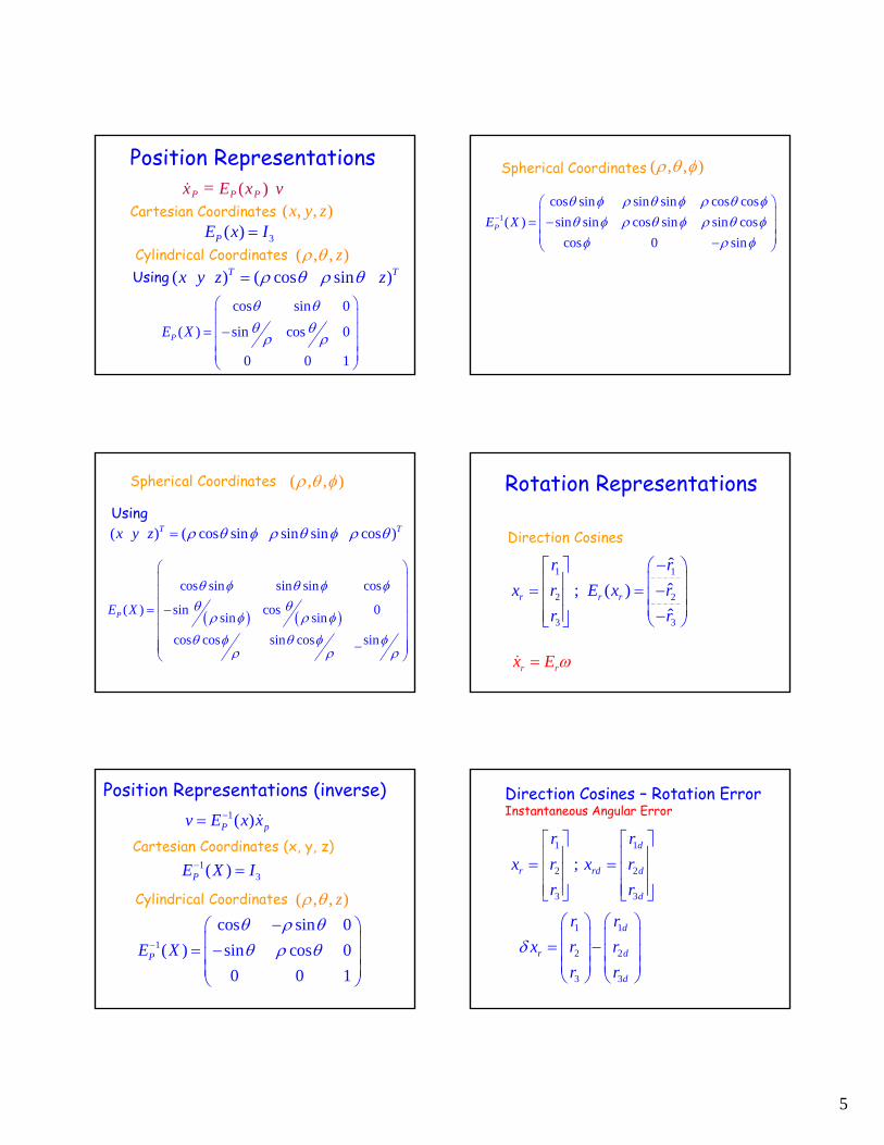
6

1

2T

rE x

1

2T

rE x

1 1

2 2

3 3

d

r d

d

r r

x r r

r r

1 1 2 2 3 3

1ˆ ˆ ˆ

2 d d dr r r r r r

desired

Instantaneous Angular Error

Euler Angles

1

0 cos sin sin

0 sin cos sin

1 0 cosr rE x

1

( ) 0

0

r

S C C CS S

E X C S

S CS S

Euler Parameters

0 1 2 3

T

rx

E 1 2 3

0 3 2

3 0 1

2 1 0

1

2E

Euler Parameters

1 0 3 2

2 3 0 1

3 2 1 0

2

r rE x

dE

( ) ( , ) ( )M q q V q q G q

Joint Space Dynamics

Centrifugal and Coriolis forces( , ) :V q q( ) :G q Gravity forces: Generalized forces

( ) :M q Mass Matrix - Kinetic Energy Matrix

:q Generalized Joint Coordinates

7

Newton-Euler Algorithm

Lagrange Equations

( )d L L

dt q q

L UK

( )U

q

d K K

dt q q

Inertial forces Gravity vector

( )U U q

Kinetic Energy

Potential Energy

Lgrangian

Since

Equations of Motion

( ) ( , ) ( )M q q V q q G q

(( )) ,M V q qq 1

2( ): TM q qMqK

( )U

q

d K K

dt q q

Equations of Motion

K m v v Ii i CT

C iT C

i ii i

1

2( )

1

n

ii

K K

vcii

Pci

Link i

Explicit Form

Total Kinetic Energy

Equations of Motion

Generalized Coordinates q

Kinetic EnergyQuadratic Form ofGeneralized Velocities

1

1(

1

2)

2 i i

nT T C

i C C i iT

ii

m v vq M q I

q

1

2Tq qK M

vcii

Pci

Link i

Explicit Form

Generalized Velocities

Equations of Motion

i ivC Jv q

1

1( )

2 i i i i

T Tv v

nT T C

i ii

m q q qJ J J JI q

Explicit Formvcii

Pci

Link i

iiC J q

1

1(

1

2)

2 i i

nT T C

i C C i iT

ii

m v vq M q I

8

Equations of Motionvcii

Pci

Link i

Explicit Form

1

2Tq qM

1

( )1

2 i i i i

nT T

i vi

T Cv imq J J I J qJ

1

( )i i i i

nT T C

i v v ii

M m J J J I J

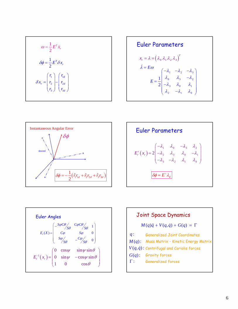
Robot Control

0k xm x

x

km

( ) ( )( ) 0

d

dt x

KV V

x

K

21

2V kx

21

2K mx

Natural SystemsConservative Forces

Natural Systems

0kxm x

V kx1

22

x

t

Frequency increaseswith stiffnessand inverse mass

n

k

m

x xn 2 0

x t c tn( ) cos( )

Natural Frequency

Conservative Forces

Dissipative Systemsx

kmx x x x Friction

Viscous friction: f bxfriction

mx bx kx 0

Natural Systems

( ) ( )( ) friction

df

dt x x

K VKV

Dissipative Systemsk

mx x x x Friction mx bx kx 0

xb

mx

k

mx 0

2 n

b

m

x

t

Oscillatorydamped

x

t

Criticallydamped

x

t

Overdamped

Higher b/m

9

n2

2d order systems mx bx kx 0

xb

mx

k

mx 0

bm

n2 n

2

Natural damping ratioCritically dampedwhenb/m=2wn

n

n

b

m

2

b

km

2

Critically damped system: n b km 1 2 ( )

Time Response x x xn n n 2 02

n

k

m ; n

b

km

2Naturalfrequency

Naturaldampingratio

x t ce tn ntn n( ) cos( ) 1 2

dampedNaturalfrequency

x(t)

t

2

1 2

n n

21 nn

1

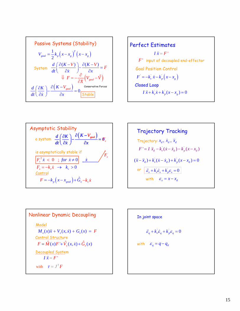
2

T

goal p g gV k x x x x

Systemd K K

dt x xf

goalV

fX

Passive Systems (Stability)

0

goalKd K

dt x x

V Stable

Conservative Forces

Asymptotic Stability

is asymptotically stable if

0 ; 0Ts x fF or x

0s v vF k kx

p goalk x xF Control

a system

x

0

goalKd K

dt x x

V goal

s

Kd K

dt x x

VF

vk x

sF

Proportional-Derivative Control (PD)mx f k x x k xp d v ( )

( ) 0v p dmx k x k x x

1. ( ) 0pvd

kkx x x x

m m

21. 2 ( ) 0dx x x x

k

mp k

k mv

p2closed loopdamping ratio

closed loopfrequency

Velocity gain Position gain

Gains

k m

k m

p

v

2

2( )Gain Selection

set

FHGIKJ

k m

k mp

v

2

2( )

k

k

p

v

2

2

Unit mass system m - mass system

k mk

k mk

p

v

k

k

p

v

10

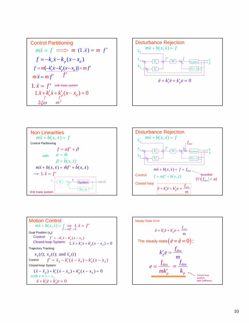
Control Partitioning

mx f (1. )x fm m

( )v p df k x k x x

fm mx f

1. x f unit mass system

1. ( ) 0v p dx k x k x x

2 2

[ ( )]v p df k x k x x fm m

Non Linearitiesmx b x x f ( , )

Control Partitioning

f f with

mx b x x mf b x x ( , ) ( , ) 1. x f

Systemf ( , )x x

++

( , )b x x

mf

Unit mass system

( , )b x x

m

Motion Controlmx b x x f ( , ) 1. x f

f mf b Goal Position (xd):

Control:

Closed-loop System: f k x k x xv p d ( )

1 0. ( )x k x k x xv p d Trajectory Tracking

x t x t x td d d( ); ( ); ( ) and Control: f x k x x k x xd v d p d ( ) ( )Closed-loop System:

( ) ( ) ( )x x k x x k x xd v d p d 0with e x xd e k e k ev p 0

e k e k ev p 0

+-

+-

+

+

xd

xd

xd

kp

kv

f m System

b x x( , )

xx

f

mx b x x f ( , ) Disturbance Rejection

Disturbance Rejectionmx b x x f ( , )

+-

+-

+

+

xd

xd

xd

kp

kv

f mf

System

b x x( , )

xx

++

fdist

mx b x x f fdist ( , )

{ } t f adist

boundedf mf b x x ( , )

e k e k ef

mv pdist

Control

Closed loop

0 :e e

k ef

mpdist

ef

mkdist

p

f

kdist

pClosed looppositiongain (stiffness)

Steady-State Error

The steady-state

e k e k ef

mv pdist

11

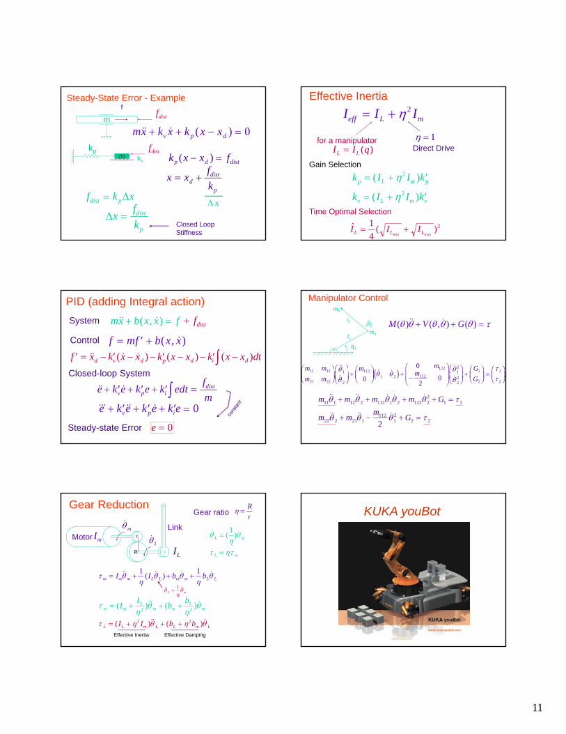
mx k x k x xv p d ( ) 0m

ffdist

kpm

x x x x kv

fdist

k x x fp d dist( )

x xf

kddist

p

xf k xdist p

xf

kdist

p

Closed LoopStiffness

Steady-State Error - Example

PID (adding Integral action)

mx b x x f ( , ) fdist

f mf b x x ( , ) zf x k x x k x x k x x dtd v d p d i d ( ) ( ) ( )

e k e k e k edtf

mv p idist z

e k e k e k ev p i 0

e 0

System

Control

Closed-loop System

Steady-state Error

R

r

Motor

m

LIm

IL

Linkr

R

Gear ratio

( )

L m

L m

1

m m m L L m m L LI I b b ( ) 1 1

L m

1

m mL

m mL

mII

bb

( ) ( ) 2 2

L L m L L m LI I b b ( ) ( ) 2 2

Effective Inertia Effective Damping

Gear Reduction

Effective Inertia

I I Ieff L m 2

for a manipulatorI I qL L ( )

1Direct Drive

Gain Selection

k I I k

k I I k

p L m p

v L m v

( )

( )

2

2

Time Optimal Selection

( )min max

I I IL L L 1

42

Manipulator Control

M V G( ) ( , ) ( )

m m

m m

m mm

G

G11 12

21 22

1

2

1121 2

122

11212

22

1

2

1

20

0

20

FHG

IKJFHGIKJ FHGIKJ

FHG

IKJFHGIKJ FHGIKJ FHGIKJ

d i

m m m m G

m mm

G

11 1 12 2 112 1 2 122 22

1 1

22 2 21 1112

12

2 22

m2

l2 q2

m1l1

q1

KUKA youBot

12

2( ) ( )[ ] ( )[ ] ( )M q q B q qq C q q G

( )p d vk q q k q

( ) sVd K K

dt q q q

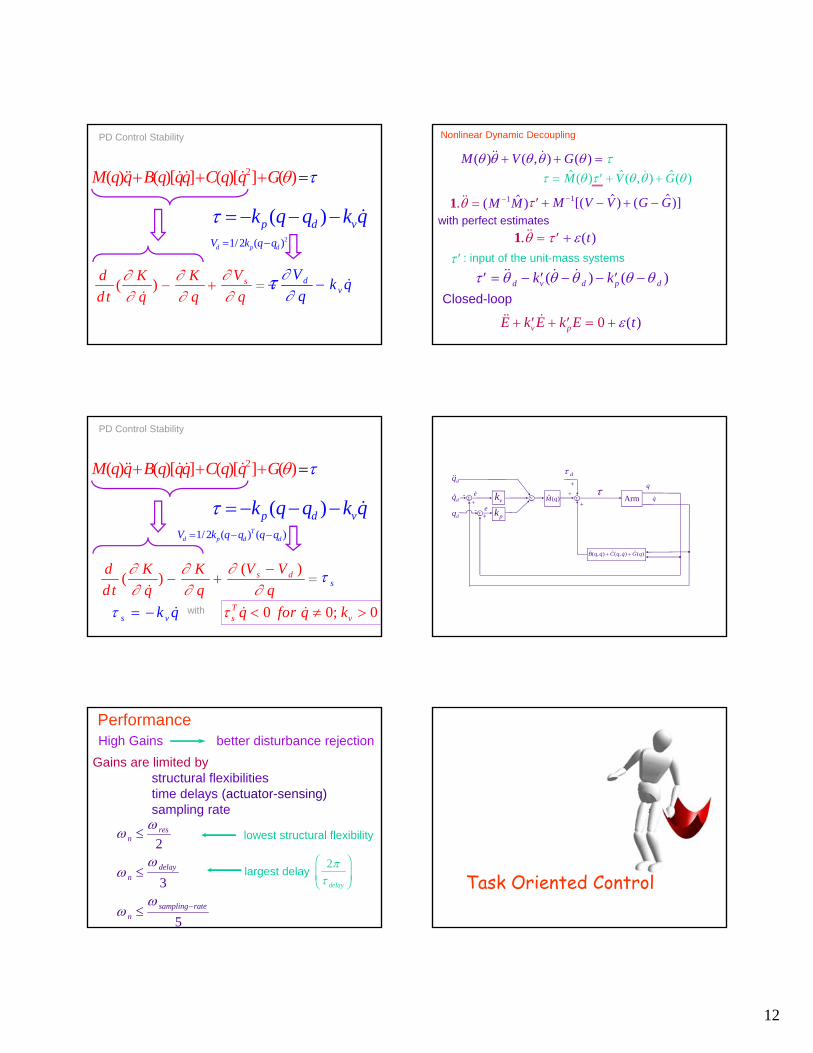
PD Control Stability

dv

Vk q

q

21/2 ( )d p dV k q q

2( ) ( )[ ] ( )[ ] ( )M q q B q qq C q q G

( )p d vk q q k q

( )( ) s dV Vd K K

dt q q q

PD Control Stability

s

1/2 ( ) ( )Td p d dV k q q q q

s vk q with 0 0; 0Ts vq for q k

PerformanceHigh Gains better disturbance rejection

Gains are limited bystructural flexibilitiestime delays (actuator-sensing)sampling rate

nres

ndelay

nsampling rate

2

3

5

lowest structural flexibility

largest delay2 delay

FHGIKJ

[( ) ( )] M V V G G1 ( )M M11.

Nonlinear Dynamic Decoupling

M V G( ) ( , ) ( ) ( ) ( , ) ( )M V G

with perfect estimates

( ) t1. : input of the unit-mass systems

( ) ( )d v d p dk k

Closed-loop

( )t E k E k Ev p 0

-

( )M q Arm

( , ) , ( )B q q C q q G q a f

kv

kp

qd

qd

qd

q

q

e

+- e

+

d

+

+

+

Task Oriented Control

13

Joint Space Control

Joint Space Control

F

( )GoalV xF

( )GoalV x

TJ F

Operational Space Control

Unified Motion & Force Control

motion contactF F F contactF

motionF

F

ˆˆ ˆ[ , , , ( )]x x x GoalM V G V xF F

x

xM x Fx xV G

Operational Space Dynamics

Task-Oriented Equations of Motion

Non-Redundant Manipulator ; n m

1 2

T

mx x x x

1 2 T

nq q q q

{0}{ 1}n

10n

14

Equations of Motiond L L

Fdt x x

with( , ) ( , ) ( )L x x K x x U x

x

y

zx

( ) ( , ) ( )x x xM x x V x x G x F

Operational Space Dynamics

End-Effector Centrifugal and Coriolis forces

( , ) :xV x x

( ) :xG x End-Effector Gravity forces:F End-Effector Generalized forces

( ) :xM x End-Effector Kinetic Energy Matrix

:x End-Effector Position andOrientation

Joint Space/Task Space Relationships

( , )xK x x 1

( )1

( )22

TTxx M x x q M q q

( , )qK q qKinetic Energy

( )x J q q Using

( )1 1

2 2T TT

x MJ M Jq q q q

where ( , ) ( )h q q J q q

1( ) () ( )( )xT M qM qq Jx J

( , ) ( )) ( )( ,( ) ,Tx xV qV x x M qqJ q h q q

( )( () )TxG J q G qx

Joint Space/Task Space Relationships

End-Effector Control

( )T FJ q F

15

1

2

T

goal p g gV k x x x x

System( ) ( )d K K

dt x

V VF

x

Passive Systems (Stability)

0

goalKd K

dt x x

V Stable

Conservative Forces

ˆgoalF V V

X

Asymptotic Stability

is asymptotically stable if

0 ; 0Ts x fF or x

0s v vF k kx

ˆp goal xx GF k x

Control

a system

x

0

goalKd K

dt x x

V goal

s

Kd K

dt x x

VF

vk x

sF

Nonlinear Dynamic Decoupling

with T FJ

( ) ( ˆˆ ˆ' , ) ( )x xx xF M F V x xG Control Structure

'I Fx Decoupled System

Model( ) ( , ) ( )x x xM x x V x x Fx G

Perfect Estimates'I Fx

input of decoupled end-effector'F

Goal Position Control

' ' 'v p gF k x k x x

Closed Loop' ' ( ) 0v p gI x k x k x x

Trajectory TrackingTrajectory: , , d d dx x x

' '' ( ) ( )d v d p dF I x k x x k x x

' '( ) ( ) ( ) 0d v d p dx x k x x k x x

with

or

x dx x

' ' 0x v x p xk k

In joint space

' ' 0q v q p qk k

with q dq q

16

Task-Oriented Control

-

( )M qx J qT a f ArmKin qa f

J qa f

( , ) ( )V q q G qx x

kv

kp

xd

xd

xd

q

q

x

xF

e

+- e

+

Compliance I x F 0 0

0 0 ( )

0 0

x

y

z

p

p d v

p

k

k x x k x

k

F

set to zero

' '

' '

'

( ) 0

( ) 0

0

v px d

v py d

v

x k x k x x

y k y k y y

z k z

Compliance along Z

Stiffness( ) 0

zv p dz k z k z z

ˆx p pM k k

determines stiffness along z

Closed-Loop Stiffness:

( )x dF K x x

J F J K x J K J KT Tx

Tx ( )

K J K JTx ( ) ( )

mf

Force Control

1-d.o.f.mx f

fd

set f fdProblem

f Nmd 1

output~0

friction

Break away

Coulomb friction10(N.m)

Force Sensing

mfdf

s

fs

s ; f k xs smx k x fs

fs

At static Equilibriumf fd f fs d

Dynamics

f fd Dynamicmx k xs

17

Dynamics

mx k x fs

m

kf f f

ss s

fm

kk f f k fd

sp s d v sf f

( ( ) )Closed Loop

m

kf k f k f f f f

ss v s p s d s df f

[ ( )]

f k x

f k x

f k x

s s

s s

s s

Control

sf

Steady-State error

m

kf k f k f f f f

ss v s p s d s df f

( ( )) ( ) 0

fdist f fs s 0

( )mk

ke f

p

sf dist

f 1

efmk

k

fdist

p

s

f

1

Task Description

Task Specification

motion forceF F F

1 0 0

0 1 0 ;

0 0 0

I

Selection matrix

Unified Motion & Force Control

Two decoupled Subsystems

*motionF *forceF

18

SystemIdentification

Conservative Systems

Natural Systems

0kxm x

V kx1

22

x

t

Frequency increaseswith stiffnessand inverse mass

n

k

m

x xn 2 0

x t c tn( ) cos( )

Natural Frequency

Dissipative Systemsx

kmx x x x Friction

Viscous friction: f bxfriction

mx bx kx 0

Natural Systems

( ) ( )( ) friction

df

dt x x

K VKV

Identificationm f

x0 xd

mx bx f ( )p d vf k x x k x

( ) ( ) 0v p dmx b x x xk k

System

Control

Closed-Loop

Time Response x x xn n n 2 02

2

pn

n

p km

k

m

2v

n

p

b k

k m

x t ce tn ntn n( ) cos( ) 1 2

x(t)

t

2

1 2

n n

x(t)

t

2