Kinematics and Momentum - SOFAD · The first learning guide is complemented by the workbook entitled ... commissions scolaires du Québec ... Collisions in Which Objects Remain Stuck

Kinematics and Momentum

PHS-5042-2

Learning Guide

NOTE

The following information is presented at the end of the guide.

• A Reader’s Comments

KINEMATICS AND MOMENTUM

PHS-5042-2LEARNING GUIDE

Kinematics and Momentum is the second of the three learning guides for theSecondary V Physics program, which comprises the following three courses:

Optics

Kinematics and Momentum

Forces and Energy

The first learning guide is complemented by the workbook entitled ExperimentalActivities of Optics, and the other two are complemented by the ExperimentalActivities of Mechanics workbook. These two workbooks cover the “experimentalmethod” component of the program.


This learning guide was produced by the Société de formation à distance descommissions scolaires du Québec (SOFAD).

Production Coordinators: Mireille Moisan (SOFAD)Jean-Simon Labrecque (SOFAD)

Coordinator: Céline Tremblay (FormaScience)

Authors: André Dumas (Chapter 1)André Manoli (Chapters 2 to 5)Suzie Asselin (Chapter 6)

Assistant to Authors: Céline Tremblay (FormaScience)

Illustrator: Gail Weil Brenner (GWB)

Content Revisors: Céline Tremblay (FormaScience)André Dumas

Translator: Claudia de Fulviis

Linguistic Revisor: Laura Yaros

Science Consultant: Janis Farrell

Layout: Daniel Rémy (I. D. Graphique inc.)

Proofreader: Gabriel Kabis

Testers: Centre l’Avenir (Mascouche)Yves Brisson (Teacher)Nancy Beauchanp (Student)Martin Bolduc (Student)Nicolas Cloutier (Student)

January 2009

© Société de formation à distance des commissions scolaires du Québec

All rights for translation and adaptation, in whole or in part, are reserved for all countries.

Any reproduction by mechanical or electronic means, including microreproduction, is

forbidden without the written permission of a duly authorized representative of the Société

de formation à distance des commissions scolaires du Québec.

Legal Deposit - 2003

Bibliothèque et Archives nationales du Québec

Bibliothèque et Archives Canada

ISBN 978-2-89493-246-9

TABLE OF CONTENTS

GENERAL INTRODUCTION

OVERVIEW ................................................................................................................... 0.12

HOW TO USE THIS LEARNING GUIDE ............................................................................. 0.12

Learning Activities ............................................................................................... 0.13

Exercises ............................................................................................................ 0.13

Self-evaluation Test ............................................................................................. 0.14

Appendices ......................................................................................................... 0.14

Materials ............................................................................................................ 0.14

CERTIFICATION ............................................................................................................. 0.14

INFORMATION FOR DISTANCE LEARNING STUDENTS ...................................................... 0.15

Work Pace .......................................................................................................... 0.15

Your Tutor ........................................................................................................... 0.15

Homework Assignments ...................................................................................... 0.16

KINEMATICS AND MOMENTUM ..................................................................................... 0.17

CHAPTER 1 – TRAJECTORIES .............................................................................. 1.1

1.1 – MECHANICS: A VAST WORLD TO EXPLORE ......................................................... 1.3

Trajectories of Different Shapes ........................................................................... 1.5

Motion, Yesterday and Today ............................................................................... 1.9

1.2 – PERCEPTION OF MOTION ..................................................................................... 1.19

A Question of Viewpoint ...................................................................................... 1.19

A Sense of Motion .............................................................................................. 1.30

Döppler Effect .................................................................................................... 1.31

Key Words in This Chapter ................................................................................... 1.43

Summary .......................................................................................................... 1.43

Review Exercises ................................................................................................ 1.45

CHAPTER 2 – DISPLACEMENT ............................................................................. 2.1

2.1 – DISTANCE TRAVELLED AND DISPLACEMENT .......................................................... 2.3

Distance ............................................................................................................. 2.4

A Question of Scale ........................................................................................... 2.7

Displacement: Setting off in the Right Direction .................................................... 2.11

2.2 – VECTORS ............................................................................................................ 2.19

Same or Not the Same? ...................................................................................... 2.20

Straight as an Arrow! .......................................................................................... 2.22

Cartesian Coordinates ........................................................................................ 2.27

Table of Contents

0.5

Straight Ahead .................................................................................................... 2.33

2.3 – VECTOR ADDITION ............................................................................................... 2.34

Polygon Method .................................................................................................. 2.40

Parallelogram Method ......................................................................................... 2.45

Component Method ............................................................................................. 2.49

Vector Resolution ......................................................................................... 2.50

Component Addition ..................................................................................... 2.54


Summary .......................................................................................................... 2.60


Note to Distance Learning Students ..................................................................... 2.68

CHAPTER 3 – SPEED AND VELOCITY ................................................................. 3.1

3.1 – SPEED: DEFINITIONS AND INTERPRETATION .......................................................... 3.3

Where Is He at Every Moment? ........................................................................... 3.5

Activity 3.1 – Keeping Track: Trajectory and Position-Time Graph .................... 3.6

What’s His Speed? ............................................................................................. 3.15

Speed and Direction ........................................................................................... 3.20

A Displacement Involving Two Velocities: A Question of Reference Points ............... 3.26

3.2 – UNIFORM RECTILINEAR MOTION .......................................................................... 3.38

In a Straight Line ................................................................................................ 3.39

Slope, Velocity and Area ...................................................................................... 3.46

An Equation That Says It All ................................................................................. 3.55

3.3 – MEASURING SPEED ............................................................................................. 3.63

The Little Train That Could: Basic Principle ........................................................... 3.63

Activity 3.2 – All Aboard! .............................................................................. 3.63

Please Be Precise ............................................................................................... 3.66

Photoelectric Cells ....................................................................................... 3.67

Stroboscopes .............................................................................................. 3.69

Spark Timers ............................................................................................... 3.72

Experimental Activity 1 – Uniform Rectilinear Motion ...................................... 3.74

How Fast Are You Going? ..................................................................................... 3.74

Sound and Light: Dizzying Speeds ........................................................................ 3.76

Speed of Sound ........................................................................................... 3.76

Speed of Light ............................................................................................. 3.78

3.4 – SPEED AND SOCIETY: MEANS OF TRANSPORTATION ............................................ 3.83

The Distant Past ................................................................................................. 3.84

The 19th Century and the Industrial Revolution ..................................................... 3.85

The 20th Century ................................................................................................. 3.89

0.6

Table of Contents

At the Dawn of the 21st Century ........................................................................... 3.93


Summary .......................................................................................................... 3.95


CHAPTER 4 – ACCELERATION .............................................................................. 4.1

4.1 – ACCELERATION: CHANGING VELOCITY .................................................................. 4.3

Coasting Down a Hill ........................................................................................... 4.3

Activity 4.1 – Faster and Faster .................................................................... 4.5

Instantaneous Velocity ........................................................................................ 4.10

An Acceleration of How Much? ............................................................................. 4.15

Acceleration With Direction .................................................................................. 4.21

Rectilinear Motion ........................................................................................ 4.21

The Acceleration Is Negative ......................................................................... 4.25

Change in Direction ...................................................................................... 4.29

4.2 – RECTILINEAR MOTION WITH UNIFORM ACCELERATION .......................................... 4.31

Graphs and Equations ......................................................................................... 4.31

Experimental Activity 2 – Rectilinear Motion With Uniform Acceleration ........... 4.40

Another Equation ................................................................................................ 4.41

A Special Case: →a = 0 ......................................................................................... 4.46

4.3 – FREE FALL .......................................................................................................... 4.48

Activity 4.2 – Falling Key Chain ..................................................................... 4.49

Gravitational Acceleration or g ............................................................................. 4.49

A Broken Fall ...................................................................................................... 4.58

Activity 4.3 – Receipt Flying Away .................................................................. 4.58

Falling on the Moon ............................................................................................ 4.63


Summary .......................................................................................................... 4.66


Note to Distance Education Students ................................................................... 4.74

CHAPTER 5 – PROJECTILES ................................................................................. 5.1

5.1 – PROJECTILE MOTION ........................................................................................... 5.3

A Non-rectilinear Trajectory .................................................................................. 5.5

Activity 5.1 – What Goes Up Must Come Down .............................................. 5.6

Motion That Is Both Horizontal and Vertical ......................................................... 5.9

Activity 5.2 – Vertical Motion and Horizontal Motion ....................................... 5.10

Equations ........................................................................................................... 5.17

Instantaneous Velocity ........................................................................................ 5.21

Table of Contents

0.7

5.2 – APPLICATIONS ..................................................................................................... 5.25

Launch Angle ...................................................................................................... 5.26

Maximum Range ................................................................................................. 5.38

Sending a Rocket Into Orbit ................................................................................ 5.39


Summary .......................................................................................................... 5.43


CHAPTER 6 – MOMENTUM ................................................................................... 6.1

6.1 – WHAT IS MOMENTUM? ........................................................................................ 6.3

Transfers in Motion ............................................................................................. 6.3

A Quantity With Direction ..................................................................................... 6.8

Experimental Activity 3 – Conservation of Momentum .................................... 6.9

6.2 – PRINCIPLE OF CONSERVATION ............................................................................. 6.10

Collisions in Which Objects Rebound .................................................................... 6.13

Collisions in Two Dimensions .............................................................................. 6.16

Collisions in Which Objects Remain Stuck Together .............................................. 6.23

6.3 – SPACE EXPLORATION ........................................................................................... 6.28

Rocket Propulsion ............................................................................................... 6.29

Dumping Stages ................................................................................................. 6.30

Correction of a Satellite’s Trajectory .................................................................... 6.32


Summary .......................................................................................................... 6.35


Note to Distance Education Students ................................................................... 6.44

CONCLUSION ........................................................................................................... C.1

SELF-EVALUATION TEST ................................................................................................ C.5

ANSWER KEY ............................................................................................................... C.23

APPENDIX A – THE INTERNATIONAL SYSTEM OF UNITS (SI) AND FORMULAS .................... C.129

Physical Quantities, Units of Measure and Symbols .............................................. C.129

Formulas ............................................................................................................ C.130

Multiples and Submultiples of SI Units ................................................................. C.130

APPENDIX B – RATIOS AND PROPORTIONS .................................................................... C.132

Ratios ................................................................................................................ C.132

Proportions ........................................................................................................ C.132

APPENDIX C – SCIENTIFIC NOTATION ............................................................................. C.134

APPENDIX D – THE LAW OF EXPONENTS ........................................................................ C.135

APPENDIX E – PYTHAGOREAN THEOREM ....................................................................... C.136

Table of Contents

0.8

APPENDIX F – PROPORTIONALITY .................................................................................. C.138

Directly Proportional Relationships ....................................................................... C.138

Inversely Proportional Relationships ..................................................................... C.139

Inverse Square Law ............................................................................................. C.140

APPENDIX G – CALCULATING TIME ................................................................................ C.141

Conversions ........................................................................................................ C.141

Converting seconds to minutes and hours ..................................................... C.141

Converting minutes to hours ......................................................................... C.142

Converting decimals to minutes and seconds ................................................. C.142

Adding Time Values ............................................................................................. C.143

Subtracting Time Values ...................................................................................... C.144

APPENDIX H – SOLVING EQUATIONS OF THE SECOND DEGREE ....................................... C.146

APPENDIX I – GEOMETRICAL PREREQUISITES ................................................................ C.147

Measuring and Constructing an Angle .................................................................. C.147

Using a protractor to measure an angle ......................................................... C.147

Using a protractor to construct an angle ........................................................ C.148

Constructing a Perpendicular ............................................................................... C.148

Various Properties of Angles ................................................................................ C.149

The Sum of the Angles of a Triangle ..................................................................... C.150

APPENDIX J – LIST OF FIGURES .................................................................................... C.152

BIBLIOGRAPHY ............................................................................................................. C.156

Books .......................................................................................................... C.156

Websites ...................................................................................................... C.156

GLOSSARY ................................................................................................................... C.157

INDEX .......................................................................................................................... C.164

Table of Contents

0.9

INTRODUCTION

OVERVIEW

Welcome to the course entitled Kinematics and Momentum, which is part of the

Secondary V Physics program. This program comprises the following three courses:

PHS-5041-2 Optics

PHS-5042-2 Kinematics and Momentum

PHS-5043-2 Forces and Energy

The three main components of the Physics program are related content, the

experimental method and the history-technology-society perspective. The experimental

method is developed in two experimental activity workbooks, while the related content

and history-technology-society perspective are covered in three learning guides

corresponding to the three courses which must be taken in sequential order.

Kinematics and Momentum is the second in the set of three learning guides. It is divided

into six chapters, corresponding to the six terminal objectives of the program.1 This

guide is to be used in conjunction with the workbook Experimental Activities of

Mechanics. You will find references to the appropriate sections of the workbook

throughout the guide.

This course will help you gain a better understanding of kinematics and momentum,

together with the related technical applications and social changes associated with

developments in this field.

HOW TO USE THIS LEARNING GUIDE

This learning guide is the main working tool for this course and has been designed

to meet the specific needs of adult students enrolled in individualized learning programs

or distance learning courses.

Each chapter covers a certain number of topics, using explanations, tables, illustrations

and exercises designed to help you master the various program objectives. A list of

key words, a summary and review exercises are included at the end of each chapter.

General Introduction

0.12

1. The terminal objectives and associated intermediate objectives are listed at the beginning of each chapter.

The conclusion contains a summary covering all the courses in the program, along

with a self-evaluation test. It also includes answer keys for the self-evaluation test,

the exercises in each chapter and the review exercises. A glossary with definitions of

the key words, a bibliography, appendices and an index are also provided in the

conclusion. You may wish to consult the books and publications in the bibliography

for further information on the topics covered in this course.

LEARNING ACTIVITIES

The guide contains theoretical sections as well as practical activities in the form of

exercises. The exercises come with an answer key.

Start by skimming through each part of the guide to familiarize yourself with the

content and main headings. Then read the theory carefully.

• Highlight the important points.

• Make notes in the margins.

• Look up new words in the dictionary.

• Summarize important passages in your own words, in your notebook.

• Study the diagrams carefully.

• Write down questions relating to ideas you don’t understand.

EXERCISES

The exercises come with an answer key, which is located in the coloured section at

the end of the guide.

• Do all the exercises.

• Read the instructions and questions carefully before writing your answers.

• Do all the exercises to the best of your ability without looking at the answer key.

Reread the questions and your answers, and revise your answers, if necessary. Then,

check your answers against the answer key and try to understand any mistakes

you made.

• To thoroughly prepare for the final evaluation, complete each chapter before doing

the corresponding review exercises, and do the exercises without referring to the

lesson you have just completed.


0.13

SELF-EVALUATION TEST

The self-evaluation test is a step that prepares you for the final evaluation. You must

complete your study of the course before attempting to do it. Reread your notebook

and the definitions of the key words in the chapters. Make sure you understand how

they relate to the course objectives listed at the beginning of each chapter. Then do

the self-evaluation test without referring to the main body of the guide or the answer

key. Compare your answers with those in the answer key and review any areas you

had difficulty with.

APPENDICES

The appendices contain a review of some concepts you should be familiar with before

beginning the course. A summary of the formulas and symbols used in this guide is

located in the appendix entitled “Formulas.” The complete list of appendices appears

in the table of contents.

MATERIALS

Have all the materials you will need close at hand:

• Study material: this guide and a notebook where you will summarize important

concepts relating to the objectives (listed in the introduction of each chapter). You

will also need to use the workbook Experimental Activities of Mechanics.

• Reference material: a dictionary.

• Miscellaneous material: a calculator, a pencil for writing your answers and notes

in your guide, a coloured pen for correcting your answers, a highlighter (or light-

coloured felt pen) to highlight important ideas, a ruler, an eraser, etc.

CERTIFICATION

To earn credits for this course, you must obtain at least 60% on the final examination,

which will be held in an adult education centre.

The evaluation for the Kinematics and Momentum course is divided into two parts.


0.14

Part I consists of a two-hour written examination made up of multiple-choice, short-

answer and essay-type questions. This part is worth 70% of your final mark and deals

with the objectives covered in this guide. You may use a calculator.

Part II is designed exclusively to evaluate the experimental method, and will consist

of a 90-minute session in the laboratory. This part is worth 30% of your final mark

and deals with the course objectives covered in the workbook entitled Experimental

Activities of Mechanics. It also includes short-answer and essay-type questions.

INFORMATION FOR DISTANCE LEARNING STUDENTS

WORK PACE

Here are some tips for organizing your work:

• Draw up a study timetable that takes into account your personality and needs, as

well as your family, work and other obligations.

• Try to study a few hours each week. You should break up your study time into several

one- or two-hour sessions.

• Do your best to stick to your study timetable.

YOUR TUTOR

Your tutor is the person who will give you any help you need throughout this course.

He or she will answer your questions and correct and comment on your homework

assignments.

Don’t hesitate to contact your tutor if you are having difficulty with the theory or

exercises, or if you need some words of encouragement to help you get through this

course. Write down your questions and get in touch with your tutor during his or

her available hours, or write to him or her. The letter included with this guide or that

you will receive shortly tells you when and how to contact your tutor.

Your tutor will assist you in your work and provide you with the advice, constructive

criticism and support that will help you complete this course successfully.


0.15

HOMEWORK ASSIGNMENTS

In this course, you will have to do three homework assignments: the first after

completing Chapter 2, the second after completing Chapter 4, and the third after

completing Chapter 6. Each homework assignment also contains questions on the

experimental method you studied in Experimental Activities of Mechanics

These assignments will show your tutor whether you understand the subject matter

and are ready to go on to the next part of the course. If your tutor feels you are not

ready to move on, he or she will indicate this on your homework assignment, providing

comments and suggestions to help you get back on track. It is important that you

read these corrections and comments carefully.

The homework assignments are similar to the examination. Since the exam will be

supervised and you will not be able to use your course notes, the best way to prepare

for it is to do your homework assignments without referring to the learning guide,

and to take note of your tutor’s corrections so that you can make any necessary

adjustments.

Remember not to send in the next assignment until you have received the corrections

for the previous one.


0.16


When we hear the word “mechanics,” we automatically think of cars, garages, expensive

repairs, engines, dirty hands, and so on. This is natural, given that cars play an

important role in our daily lives and we often need them in order to travel from place

to place. In physics, the term “mechanics” has a broader meaning. It describes motion

and the actions that give rise to or influence it. The word mechanics is derived from

the Greek mékhané, meaning machine.

Mechanics is the branch of physics that studies motion; for the most part, it describes

motion quantitatively through the use of graphs and equations. This is the focus of

kinematics (from the Greek word kinêmaticos, meaning motion). This science makes

it possible, for instance, to analyze post-race performance of cars, predict the future

position of planets in the sky or determine how long it takes to get from Chicoutimi

to Québec City or from Montréal to Ottawa.

Mechanical physics also studies the causes or forces that give rise to motion or change

the course of objects in motion. How can we move an object that is stationary or in

equilibrium? Why does the Earth revolve around the Sun? How can a lever or a pulley

help lift heavy loads? How can we change the path of a satellite, a skydiver or a nuclear

warhead? The science that studies the relationship between forces and motion is called

dynamics (from the Greek dunamikos, meaning power). This branch of physics

examines the forces that produce or change motion, and the energy associated with

them. It also explains the motion of a bicycle, car or crane through a series of

mechanical parts or simple machines such as levers, pulleys and gear systems.

Optics, the first course in the Secondary V Physics program, dealt with light, its

propagation and its interaction with mirrors, lenses or prisms. It ended with an analysis

of the nature of light and the behaviour of colours. The other two courses, the one

you are about to begin and the next, are devoted to mechanics. This course,

Kinematics and Momentum, deals mainly with the mathematical description of motion

(kinematics), whereas Forces and Energy focuses on the causes of and changes in

motion, as well as the use of simple machines (dynamics). Let’s look more closely at

the contents of this guide.


0.17

Chapter 1 will familiarize you with the concept of trajectory, or the path of an object

in motion, and its representation. You will also learn about reference points, since

the description of a motion depends on our point of view. For example, the same motion

can be seen as either a straight line or a curve, depending on the observer’s position.

The chapter also discusses how we can detect motion through hearing, smell and

touch, which provide valuable information that complements visual perception. A

brief look at history reveals that motion did not always have the same explanation

it has today, and that its history is marked by important milestones, dominated by

major figures such as Aristotle, Galileo, Newton and Einstein.

In Chapter 2, you will explore the concepts of displacement and distance travelled,

in the physical sense of these terms. You will also be introduced to vectors, a

mathematical tool used to provide a complete description of displacement. Vectors

are characterized by both a magnitude, or the distance between the start and finish

points, and by a direction—that of the straight line connecting these points.

Chapter 3 deals with speed, velocity and the velocity vector. Uniform rectilinear motion,

or motion in a straight line and at constant velocity, is analyzed in detail. You will

also learn to describe motion, using graphs and equations, and to measure velocity.

The chapter ends with a discussion of the evolution of transportation and the influence

of speed on society.

Chapter 4 examines acceleration, or changes in velocity. You will study uniformly

accelerated rectilinear motion or motion in a straight line, with constant acceleration.

Graphs, equations and vectors will describe, for instance, the motion of a car from

rest to its cruising speed, or over a braking distance. We will also discuss gravitational

acceleration, which results from the force of gravity that keeps us on the ground, causes

apples to fall and keeps the Moon in its orbit.

Chapter 5 is devoted to projectiles such as bullets, arrows or baseballs, whose motion

occurs in a plane, unlike the previous examples, whose trajectory is linear.

Mathematical tools are extremely valuable in determining, for instance, where a

projectile will land, how high it will rise, and so on. The chapter ends with a look at

how knowledge of projectile trajectories evolved over time.


0.18

The sixth and last chapter examines momentum, which is a measure of the mass and

velocity of a moving object. Its total value is conserved (constant) in a system comprised

of two or more objects, provided no outside force acts on the system. Using this

principle of conservation, we can predict things like the direction in which two billiard

balls will roll after colliding. The study of momentum opens the door to dynamics,

which centres on the concept of force, and will be examined in detail in the next course.

The overall layout of this guide is similar to that of the preceding one. Each chapter

begins with a list of objectives, followed by a table of contents diagram showing how

the chapter fits into the course as a whole. This diagram outlines the topics covered

in each chapter. The table of contents diagram for Chapter 2 is reproduced below.

The topics in the chapter you are about to begin (Chapter 2) are in bold type, while

those of the completed chapter (Chapter 1) are in italics. The topics in upcoming

chapters (Chapters 3 to 6) are in regular type.

Table of contents diagram appearing at the beginning of Chapter 2

END

3. Speed and Velocity

Position-time graph

Scalar speed and velocity vector

Adding velocities

Uniform rectilinear motion

Measuring velocity

Rapid transportation and society

2. DisplacementDistance covered

Displacement vector

Vector addition: 3 methods

5. Projectiles

Trajectory

x and y components

Applications

A little history

4. Acceleration

Instantaneous velocity

Acceleration vector

Uniformly accelerated rectilinear motion

Comparing constant a and constant v

Gravitational acceleration

6. Momentum

Momentum (p)

Conservation of p

Elastic and inelastic collisions

Applications

1. Trajectories

Different types of trajectories

Motion

A little history

Perception of motion

Döppler Effect

KIN

EM

ATIC

S AND MOMEN

TUM


0.19

We recommend that you refer to it often to see where you are in the course. You will

soon discover that it is a very effective working tool that will help you recall the concepts

covered in the various chapters.

Have fun!


0.20

CHAPTER 1

TRAJECTORIES

GWB

Terminal Objective 1

To analyze the concept of trajectory and the perception of motion.

Intermediate Objectives

1.1 To give examples of motion at different levels.

1.2 To place in historical perspective the scope of subjects covered in mechanics.

1.3 To associate discoveries about the motion of heavenly bodies with the evolution of human perceptionof the universe.

1.4 To define the concept of trajectory.

1.5 To classify different types of motion according to their trajectories.

1.6 To illustrate that the perception of motion and immobility depends on the point of view of the observer,using examples.

1.7 To describe the perception of various motions by means of the senses, using examples.

1.8 To solve problems related to the concept of trajectory and the perception of motion.

Kinematics and Momentum – Chapter 1: Trajectories

END

3. Speed and Velocity

Position-time graph

Scalar speed and velocity vector

Adding velocities

Uniform rectilinear motion

Measuring velocity

Rapid transportation and society

2. Displacement

Distance covered

Displacement vector

Vector addition: 3 methods

5. Projectiles

Trajectory

x and y components

Applications

A little history

4. Acceleration

Instantaneous velocity

Acceleration vector

Uniformly accelerated rectilinear motion

Comparing constant a and constant v

Gravitational acceleration

6. Momentum

Momentum (p)

Conservation of p

Elastic and inelastic collisions

Applications

1. TrajectoriesDifferent types of trajectories

Motion

A little history

Perception of motion

Döppler Effect

KIN

EM

ATIC

S AND MOMEN

TUM

On July 20, 1969, Americans Neil Armstrong and Edwin Aldrin became the first

astronauts to walk on the Moon. It took exact calculations to plan the various stages

of the spacecraft’s voyage, send the command module into orbit around the Moon

and have the lunar module land at the desired location. Closer to home, other devices

have been designed to facilitate locomotion: ice skates, bicycles, airplanes, automobiles

and boats. Life is intimately linked to motion. Birds fly, fish swim, people walk and

run. Inanimate matter also exhibits motion: winds, tides, rain and snow, flowing brooks,

rivers and streams are a few examples.

In this chapter, we will examine motion by first defining the concept of trajectory and

describing the various types of trajectories. We will also look at how theories of motion

have evolved over time. You will see how some of our perceptions today resemble the

ideas of Aristotle, who lived more than 2 000 years ago. We will also explore a few

branches of mechanics and learn that the description of a motion depends on the

observer’s reference point. The chapter will close with an analysis of the Döppler effect,

which explains the changes we hear in noise coming from a moving source, such as

an ambulance siren, relative to an observer who is stationary.

1.1 – MECHANICS: A VAST WORLD TO EXPLORE

As mentioned in the general introduction to this learning guide, mechanics refers not

only to what is under the hood of a car. It is also a branch of physics that studies motion

and takes in a wide range of theoretical knowledge and technical applications. But

what exactly is motion? You may answer that it is obviously anything that moves. But

what parameters are involved in motion? Let’s start by looking at a specific example.

We will take a short car trip and examine motion at different points along the way.

Imagine you are behind the steering wheel of a car, driving either in the country or

in the city. The drive is pleasant and nothing of any consequence is happening. Yet,

a number of events along the way necessitate certain actions.


1.3

Exercise 1.1

Complete the following list by naming five actions relating to the car’s motion.

Going uphill, decreasing speed,

Driving manoeuvres depend on the shape of the trajectory, road signs and any

obstacles along the way. They can affect the velocity (e.g. acceleration, deceleration,

braking, travelling at a constant speed) or the direction (e.g. negotiating a curve, going

uphill or downhill).

Exercise 1.2

In the following diagram of an automobile racing circuit, the arrows indicate the

direction of the race. Identify the type of manoeuvre relating to the velocity that is

likely to occur when the car passes each numbered point. More than one manoeuvre

may be possible at each point.


1.4

?

?

The manoeuvres listed in the previous two exercises already tell us a great deal. First,

they indicate that motion is associated with velocity, which can either remain

constant, increase, decrease or drop to zero, depending on whether the car is cruising

accelerating, slowing down or stopping. It also shows that the motion involves a direction

that can change depending on whether the car is going uphill, downhill or around a

bend.

The example of the car shows how much motion can vary. One way to categorize the

different types of motions is by changes in velocity. For example, we speak of uniformmotion1 if the velocity is constant and accelerated motion if the velocity changes. Motion

can also be categorized according to the type of trajectory, and this is what we will

be examining in the following section.

TRAJECTORIES OF DIFFERENT SHAPES

Motion is generally described according to the shape of the path taken by the moving

object, in other words, its trajectory. More specifically, trajectory is defined as the

curve described by a moving object. We refer to rectilinear motion when an object

moves along a straight line and to non-rectilinear motion in other cases.

The figure below shows what happens when the string of the plumbline on the right

is cut. As it falls, the plumb bob occupies successive positions that describe its

trajectory—a vertical line as straight as that of the plumbline on the left. A trajectory

is therefore the line of imaginary points that mark the successive positions occupied

by a moving object.

Figure 1.1 – Rectilinear trajectory

All of the successive positions occupied by the falling plumb bob on the right describe a vertical rectilinear trajectory.

$


1.5

1. Words appearing in bold type are defined in the glossary found at the back of the learning guide.

Like the plumb bob in Figure 1.1, an apple falls from a tree in a straight vertical line,

that is, its motion is rectilinear. But not all motion is rectilinear. For instance, a car

follows the curve of the road in a non-rectilinear motion, and the path of Earth as it

revolves around the Sun forms an ellipse. Because so many types of trajectories are

possible, they are referred to by their shape. The general term curvilinear trajectorydesignates a path with one or more curves. We refer to a circular trajectory when the

motion of the object describes a circle, an elliptical trajectory when it describes an

ellipse, or a parabolic trajectorywhen it describes a parabola. A random trajectory

means that the motion describes no definite shape.

Exercise 1.3

For each of the following drawings, use a word to describe the trajectory.

a) b)

_________________________________ _________________________________

c) d)

_________________________________ _________________________________

e)

_________________________________

x

45°

y


1.6

?

A stone whirled in a sling describes a circular trajectory, a satellite’s orbit describes

an elliptical trajectory and an archer’s arrow follows a parabolic trajectory. The various

types of trajectories are summarized in the table below.

Figure 1.2 – Types of trajectories

A random trajectory often comprises specific segments whose shapes correspond to

one of the types of trajectories described above. It can therefore be divided into its

component trajectories. For example, a space shuttle describes a trajectory that can

be broken down into two stages. After it is launched, it first follows a rectilinear trajectory

and, immediately after ignition, the craft begins a curvilinear trajectory.

Figure 1.3 – Trajectory of a space shuttle

The trajectory of a shuttle is made up of a vertical rectilinear trajectory followed by a curvilinear trajectory.

Type of trajectory Symbol Examples

Rectilinear A car travelling on a straight road

Circular A pedal rotating on a bicycle

Elliptical A planet orbiting the Sun

Parabolic An arrow shot by an archer

Random A driver’s route in travelling from one place toanother


1.7

Exercise 1.4

Some of the types of motion you are likely to observe in your environment are listed

below. For each one, indicate the type of trajectory involved.

a) The light beam from a flashlight _______________

b) The rotation of a truck wheel _______________

c) A child chasing a butterfly _______________

d) A football kicked at 30° to the horizontal _______________

e) A hockey puck passed from one player to another _______________

f) The blade of a fan _______________

g) Earth’s motion around the Sun _______________

h) A firefly in the dark _______________

To summarize, different types of motions can be categorized according to changes in

their velocity or the shape of their trajectory. The following diagram combines these

two aspects. Take the time to study it, as these terms occur frequently throughout the

guide.

Figure 1.4 – Different types of motion

Motion can be described as rectilinear or non-rectilinear depending on the type of trajectory.Rectilinear motion can be further subdivided depending on the type of velocity involved. Non-rectilinear trajectories can be curvilinear (circular, elliptical, parabolic) or random.

Motion

Rectilinear Non-rectilinearmotion motion

Constant Variable CurvilinearRandom

velocity velocity • parabolic

(uniform (non-uniform • circular

rectilinear rectilinear • elliptical

motion) motion)

Constant Otheracceleration

(rectilinear

motion with

uniform

acceleration)


1.8

?

Different types of motion are characterized by the velocity of the object and the shape

of the path it describes. But do all objects behave in the same manner, regardless of

their trajectory?

It is a given that motion is everywhere: in an apple falling to the ground, the blood

flowing through our veins, a child skipping rope, a butterfly hovering around a flower,

the blades of a whirring fan and the bus that takes us to work. Motion can also be

invisible, for example, in minuscule organisms such as bacteria, molecules and

atoms, or if the displacement is minimal. At the other extreme, motion can also assume

gigantic proportions, as in the case of the planets orbiting the Sun or the evolution

of stars and galaxies.

Exercise 1.5

Give three examples of moving objects or situations associated with each scale

indicated.

Astronomical scale: __________________________________________________________

Human scale: ________________________________________________________________

Microscopic scale or smaller: _________________________________________________

We are aware of the vibratory motion of atoms within molecules, and we know that

the Moon revolves around Earth, which in turn revolves around the Sun. This

knowledge is relatively recent, but the study of motion is centuries old. In ancient times,

the concepts of motion and velocity were interpreted differently than they are today,

and in the next section you will learn how these concepts evolved.

MOTION, YESTERDAY AND TODAY

Throughout history, people have been fascinated by motion. It is an inextricable part

of life. Consider the invention of the wheel and the development of such tools as the

lever, wheelbarrow, pulley and gear. These implements make lifting or carrying

objects easier and enable us to accomplish tasks that would otherwise be difficult or

impossible.


1.9

?

In the following overview, we will emphasize the theoretical aspects of motion and

examine how ideas evolved in this regard. We will look at three important figures,

namely Greek philosopher Aristotle (384-322 B.C.), Italian mathematician and

physicist Galileo Galilei (1564-1642) and English mathematician and physicist Sir Isaac

Newton (1642-1727).

We’ll begin by looking at how Aristotle conceived the physics of motion more than

2300 years ago. This great thinker saw things very differently from the way we do today.

In his perception, the natural state of objects was to be stationary, and motion was a

transitional state between two positions of an object at rest.

Aristotle considered that according to the laws of nature, every object has a natural

place to which it tends to return, if it is not already there—where it will remain once

it reaches this place. Thus, Aristotle theorized that an apple falling to the ground or

a stone rolling down a slope are both seeking to return to their natural place.

Likewise, the weight of a stone in our hand is an expression of the stone’s attraction

to the ground, its natural place.

Figure 1.5 – Natural motion according to Aristotle

According to Aristotle, the stone rolls down the slope because it is “programmed” by an internalcharacteristic to roll downward and reach its natural position at rest.

In these examples, the objects move on their own toward the ground; this is why Aristotle

spoke of natural motion. But how can we explain that a stone thrown upward rises

before falling to the ground? He believed that the stone, projected upward, follows

an unnatural motion by rising, because it moves away from its natural place of rest.

It is a violent motion upward, because it is the result of a forced action. The air pushes

the stone upward; however, as the stone rises, the force of the air becomes weaker

and the stone eventually falls to the ground.


1.10

Figure 1.6 – Natural motion and violent motion

a) Why does the stone not fall immediately after being thrown?

b) According to Aristotle, the air causes the stone to rise. As the stone rises, the force of the air on the stone steadily weakens and the stone falls.

To Aristotle and those who came after him, velocity was an intuitive concept, with no

mathematical definition, units of measure or numerical values. It served to compare,

for example, two runners competing against each other. They start at the same time,

and the first to reach the finish line is faster. The concept of record-keeping did not

exist, and the results of one race were not compared to other races. Furthermore,

observation was not the starting point for theory development. Observation, like

experimentation, could not be trusted because the imperfect nature of humans

provided a false perception of reality, which was governed by a perfect or divine cosmic

order.

These ideas seem rather astonishing today, but Aristotle’s theories prevailed for

almost two thousand years because many of these theories were elevated to the status

of dogma by the Roman Catholic Church. It was better to accept them than to question

them, as Galileo unfortunately learned in the early 1600’s.

a) b)

Gust of wind

?


1.11

In the 17th century, Italian physicist Galileo stated that the Earth and the other planets revolved around the

Sun. His view ran counter to Aristotle’s model, in which the Earth was the centre of the universe. Church officials

refused to question the prevailing beliefs about the nature of the universe. On June 22, 1633, the Inquisition2

condemned Galileo. He was forced to renounce his teachings and to reaffirm the “truth.” Here is what he

apparently said in order to save his life: “I, Galileo Galilei, professor of physics and mathematics at the University

of Florence, renounce what I have taught, namely that the Sun is at the centre of the Universe and immoveable,

and that the Earth is not the centre and that it moves. I abjure with sincere heart and unfeigned faith, I curse

and detest the said errors and heresies, and, generally all and every error and false opinion contrary to the

Holy Catholic Church. Then, without being overheard by those judging him he is reputed to have said: “Eppur

si muove!” which means “But still it moves.”

Galileo was then sent back to his native city and lived under surveillance and near seclusion until his death.

He was allowed the one privilege of visiting the convent near his villa. He died in 1642, the year Isaac Newton

was born. He too had a great impact on the physics of motion.

In 1992, more than 350 years later, the Roman Catholic Church, through Pope John Paul II, finally apologized

to the scientific community for the injustice done to Galileo.

In the 17th century, Aristotle’s theories were still widely accepted, and experimentation

was not trusted as a source of knowledge. But Galileo helped to bring about change.

He may not have invented experimentation, as some maintain, but he was the first

to validate it. His work is distinguished by elaborate and detailed experiments,

reproducible results and clear conclusions. To him, experimental science was the frame

of reference: observations must correspond to the theory, otherwise the theory must

be altered or discarded.

Galileo’s best-known experiment involved comparing the time it took two objects of

different masses to fall. He dropped two balls of similar shape but different masses

from the top of Italy’s Tower of Pisa (Figure 1.7).

And Yet It Moves


1.12

2. The Inquisition was instituted by Pope Gregory IX in the early 1200s. This ecclesiastical institution had legal powersand was mandated to combat heresy and apostasy, sorcery and witchcraft throughout Christendom. Theinquisitorial proceedings resulted in thousands of people being burned at the stake, in some cases, after havingbeen tortured. Considered a special tribunal, the Inquisition remained influential nonetheless, until the 1600s.

Figure 1.7 – Falling objects

a) Two balls of the same size but different mass are released from the top of the Tower of Pisa. In your opinion, what will happen when they reach the ground?

b) If you had witnessed the experiment, you would have heard only one sound, since the two ballshit the ground at the same time. You may have been as surprised as Galileo’s contemporaries.

c) In the tube on the left, the feather falls more slowly than the marble, since it is slowed down by the air in the tube. On the right, when a vacuum is created in the tube,

the feather falls at the same velocity as the marble.

If we were to repeat the experiment, we would observe that the two balls in Figure

17a) reach the ground simultaneously every time. The experiment is therefore

reproducible and contradicts Aristotle’s theory, which maintained that heavy objects

fall faster than light ones. It is true that a feather or a piece of paper, light enough to

be carried by the air, falls more slowly than a stone. However, if we eliminate the effect

of the air by creating a vacuum inside a tube, all objects fall at the same velocity,

regardless of their mass or shape (Figure 1.7c).3

Thanks to Galileo, the antiquated concept of motion was laid to rest. He asserted that

motion is not an intrinsic property of an object, in other words, the object is not

“programmed” to seek its “natural place of rest,” and that motion does not affect its

nature. Rather, motion has to do with the position of an object and its change over

time relative to another object that serves as a reference point. Galileo therefore

transformed the concept of motion. He was a pioneer in experimentation, and

precisely defined planetary motion and the motion of objects, such as a falling apple

or the trajectory of an arrow shot by an archer.

a) b)

wooden balllead ball

c)


1.13

3. Try this experiment yourself. Pose the problem to some of your friends or family members who have not studiedphysics. Some will probably answer that the heavier an object the faster it will fall. You could explain to themwhat actually happens, or better yet, perform the experiment.

Inspired by the work of René Descartes (1596-1650), Galileo believed that a moving

object has constant velocity as long as it is not acted upon by factors such as the

roughness of the surface on which it moves, an obstacle or the attraction exerted by

another object.

Isaac Newton (1642-1727) restated Galileo’s principle of inertia in his own terms and

expressed it this way: “Every object will continue in a state of rest or with constant

speed in a straight line unless acted upon by an external unbalanced or net force.”4

In other words, a stationary object tends to stay at rest unless it is acted upon by an

external force; likewise, a moving object tends to keep moving at a constant speed in

a straight line provided it is not acted upon by any external forces.

Newton went further in explaining the motion of objects by introducing the concept

of force. He also related the effects observed by Galileo to the causes that produce

them. Objects fall because the Earth exerts a force of attraction on them. The Moon

is also attracted by the Earth; this is why the Moon remains in its orbit around the

Earth.

Before Newton, it was assumed, as did Aristotle, that the motion of celestial bodies

was governed by laws different from those governing the falling apple or the archer’s

arrow. Newton revolutionized physics by asserting that the same cause explains the

Moon’s motion and an object’s fall, and he proved his theory mathematically. The

mechanics of celestial bodies, dealing with astronomical observations, and terrestrial

mechanics, concerning motion on the human scale, were now governed by laws known

as Newton’s Laws of Motion.5

Newton first established the laws for falling objects on Earth. In 1665, he extended

their application to the motion of celestial bodies such as the Moon and the planets.

The well-known story credits him with having a flash of intuition when he watched

an apple falling from a tree. As a result, Newton formulated the Law of Universal

Gravitation, which explains both the falling apple and the motion of the Moon. The

law also explains why the Earth is flattened at the poles. If facilitated the calculation

of making possible to calculate the path of Halley’s Comet, which orbits the Earth

every 76 years,6 and led to the discovery of Neptune and Pluto,7 the most remote planets

in the solar system.


1.14

4. Forces external to the object may be forces due to friction, the force of attraction between objects or a physicalor mechanical force.

5. Newton’s Laws of Motion will be covered in detail in the next course in this series, Forces and Energy.

6. Halley’s Comet was visible in 1986 and is expected to be visible again in 2062.

7. Disturbances in the orbit of Uranus alerted scientists to the presence of Neptune, first located in 1845 by FrenchmanLe Verrier, and that of Pluto, discovered in 1930 by American Clyde Tombaugh.

Figure 1.8 – Newton’s apple

What is the relationship between the motion of an apple falling to the ground and that of the Moon as it orbits around Earth? Under Earth’s attraction,

the Moon “falls” relative to a straight-line motion.

Solitary, austere, driven and intellectually ambitious, Newton was sensitive to criticism.

He waited 22 years before presenting his discovery of the Law of Universal Gravitation,

and did so under the auspices of his former colleagues. He was a perfectionist, did

not easily accept preconceived ideas and supported his conclusions with rigorous

experiments.

The work of Galileo and Newton is part of modern science, and their conclusions are

still valid, although their current wording is simpler than the original. Galileo

precisely described the trajectory of objects that fall and that of planets and their natural

satellites (their moons). Today his results are included in basic textbooks, such as this

learning guide, which deal with kinematics, the science that describes the motion of

objects. Newton’s work on gravity explains the causes of the motions described by

Galileo. His laws are taught in all introductory courses in dynamics, the branch ofphysics that deals with the causes of motion. Kinematics and dynamics are two major

branches of mechanical physics.


1.15

You may be wondering what advances have been made in the field of mechanics since

the 17th century, the era in which Galileo and Newton transformed mechanics. Do their

theories apply to all types of motion, regardless of the velocity and size of the objects

involved? Let’s see.

Clearly, science has advanced rapidly since the 17th century. Better mathematical tools,

progress in the field of metallurgy and the development of new materials are only a

few elements that have facilitated this growth in technical applications as they

pertain to mechanics. The theoretical component of this science has also evolved

significantly. Because of the vast scope of topics encompassed by mechanics, this field

has been subdivided into several branches, all having to do with the study of motion,

but dealing with a specific area and clearly defined conditions.

Classical mechanics, generally associated with the work of Galileo and Newton, attempts

to describe and interpret current phenomena. Its laws are valid when the speed of

objects is low relative to that of light.8 Its field of application is vast and includes the

motion of planets and the archer’s arrow, as well as motion on a smaller scale, such

as the motion of the molecules in a gas. On the other hand, it cannot predict the

behaviour of subatomic particles, such as electrons or protons, which may attain speeds

close to that of light.

Fluid mechanics is the study of the motion of fluids (liquids and gases). Besides the

theoretical component, fluid mechanics has many applications, such as the hydraulics

of automobile transmission and brake systems, the presses used to mould metal or

plastics, or the design of airplane wings, since the flow of air around the wing is key

to the craft’s performance. We will have a chance to explore this topic when we look

at Archimedes’ Principle in the next course.

Thermodynamics, also known as the mechanics of heat, is the study of heat and its

interaction with matter. Among other things, it deals with the relationship between

heat and motion, which led to the invention of the steam engine and, a little later, to

the internal combustion engine.


1.16

8. The speed of light, designated as c, is 300 000 km/s.

Relativistic mechanics is the study of the motion of objects that move at speeds

comparable to the speed of light, which cannot be explained in terms of classical

mechanics. Subatomic particles (e.g. protons and electrons) can attain speeds of this

magnitude in particle accelerators, solar winds or in the proximity of black holes. The

laws of relativistic mechanics were developed by the German physicist Albert Einstein

(1879-1955), when he presented the first version of his theory of relativity at age 26.

Relativity called into question existing concepts of space and time. For example, time

passes differently depending on whether we are stationary or moving at a speed close

to that of light. For an observer moving at a speed near the speed of light, time passes

more slowly, objects shrink and their mass increases.

According to Einstein, time passes more slowly when an object moves at high speed.

Atomic clocks are high-precision timepieces that measure billionths of a second. In 1971, scientists used this

type of clock to verify Einstein’s theory by placing one aboard an airplane flying at 966 km/h around the Earth.

A second clock remained on the ground. At the beginning of the experiment, the two clocks showed the same

time. On the airplane’s return, the first clock indicated a time lag of a few billionths of a second.

But, you might say, why so little difference? To us, 966 km/h may seem fast, but it is slow compared with the

speed of light, which is 300 000 km/s. In order to record a noticeable time difference, the airplane would

have had to travel at a speed comparable to that of light.

Quantum mechanics is based on quantum theory, which holds that energy is

transmitted in small indivisible units called quanta. It evolved from the failure of classical

concepts about waves and particles to describe phenomena occurring at the atomic

and subatomic levels. Attempts to apply the laws of classical mechanics to the

behaviour of matter at the atomic level had been futile. Quantum mechanics was first

applied to light, then to atomic physics. For instance, it explains how an electron behaves

in the electronic cloud of an atom. The electron, like light, sometimes acts like a particle

and sometimes like a wave. If you are perplexed, it is because these concepts are difficult

to grasp, since there is no adequate everyday example to explain them.

Time Dilation


1.17

Exercise 1.6

1. Match each situation in the list below with the corresponding branch of mechanics.

Write the number between the parentheses at the end of each phrase.

Branches of mechanics:

1) Classical mechanics (dynamics) 4) Quantum mechanics

2) Classical mechanics (kinematics) 5) Fluid mechanics

3) Relativistic mechanics

Situation:

a) The trajectory of Halley’s Comet ( )

b) The motion of electrons around the nucleus of an atom ( )

c) The orbit of the Earth around the Sun ( )

d) An electron can be considered a wave ( )

e) The distance travelled by a car ( )

f) The description of the motion of the planets around the Sun ( )

g) Time passes more slowly at speeds close to that of light ( )

h) The pressure exerted by water on an immersed object increases

with the depth ( )

i) A hockey puck is struck to accelerate its motion ( )

Mechanics encompasses several branches, some of which appear very complex and

will not be covered in this course. Keep in mind that motion is the common

denominator in all of these branches and that this guide is devoted for the most part

to classical kinematics, one of the main branches of classical mechanics. Let’s return

to the concept of trajectory and see how the description of a trajectory can depend

on how we perceive it.


1.18

?

1.2 – PERCEPTION OF MOTION

Consider the following example. Two cars collide at a busy intersection. The police

officer investigating the accident questions two witnesses who saw the accident from

two different angles. According to one, the back of the white car skidded before the

collision. He also said that the black car was going too fast. According to the second

witness, no skidding occurred, and the black car was moving at a reasonable speed,

below the maximum limit.

While subjectivity plays an important role, this example shows that the way in which

a scene in motion is perceived can depend on the viewpoint of the observer, both with

respect to the velocity of the objects involved and their trajectories. This perception

differs even if the observers are completely objective. We will explore this idea in more

detail below.

A QUESTION OF VIEWPOINT

The way we describe a trajectory depends on our viewpoint. Once again, consider the

motion of the planets. We now know that they revolve around the Sun, along elliptical

orbits or trajectories. This is what an observer outside the solar system would see.

Figure 1.9 – Solar system

If we observed the planets revolving around the Sun from a point outside the solar system, their orbits would appear elliptical.

Sun Venus

Mercury

Mars

Earth

Jupiter

Saturn

Uranus

Neptune

Pluto


1.19

We are accustomed to seeing the solar system depicted in this way. Although this view

is correct, it does not entirely correspond with what we observe from the Earth’s surface.

Aristotle believed that the Earth remained in place at the centre of the universe.

Exercise 1.7

The figure below shows the position of the Sun at different times during the day, as

observed from Earth.

a) Describe the motion of the Sun, as perceived from the Earth’s surface.

b) Describe the motion of the stars, from dusk until dawn.

c) Does it seem to you that the Earth is moving?

d) Does it seem to you that the Earth rotates on its own axis?

e) Why did Aristotle think that the Earth was the centre of the universe?

East West

Horizon


1.20

?

Aristotle’s perception of the universe is not that far-fetched when we consider that he

saw the Sun move across the sky from morning to night, that he did not have a telescope

and that outer space was inaccessible to him. A few centuries later, Greek astronomer

Ptolemy (85-160) observed the position of certain planets each evening and noted that

they move in one direction, but occasionally they reverse their direction (retrogrademotion), as though they were moving backward for a time before resuming their

forward motion.

Figure 1.10 – Mars’ apparent retrograde motion

Apparent motion of the planet Mars, as observed from Earth over a period of a few months.Ptolemy had observed the retrograde motion of planets and tried to explain it

using a geocentric model (see below).

According to Aristotle, each planet occupies a fixed position in its own sphere around the Earth. The spheres

revolve around the Earth, the centre of the universe. Since each celestial body occupies a natural position,

why do they not fall to a position of rest, like objects on the Earth’s surface? Aristotle’s explanation was that

celestial bodies do not fall because their motion is governed by different laws from those that govern the motion

of objects on Earth. The natural state of objects on Earth is to remain at rest, and that of celestial bodies to

remain in perpetual circular motion.

Aristotle’s and Ptolemy’s Geocentric Universe

7

7 66

5

54

4

3

3

22

1

1

Mars moveseast again

Mars’ orbit

West

East

Earth’sorbit

}

Mars moveseast}

Mars moveswesttemporarily

}


1.21

Aristotle’s model of the universe

Aristotle placed the Earth at the centre of the universe, since it was a given that, as intelligentbeings, humans occupied a central position in the overall scheme of things. This model is said to be geocentric (“geo” from the Greek “gê”, meaning “earth”). When the Earth turns on its own

axis, it pulls celestial bodies along with it, and these maintain their original positions.

Ptolemy’s geocentric model

Ptolemy’s model was based on observations with the naked eye. He tried to explain the retrogrademotion of planets within the geocentric model by introducing a small circular motion

that is superimposed on the circular orbit.

TerreEarth

Moon Mercury

Venus

Sun Mars

JupiterSaturn

Fixed stars

Earth Moon

Mercury

Venus

Sun

Mars

Jupiter

SaturnCelestial sphere


1.22

Nearly 1400 years after Ptolemy, Polish astronomer Nicolas Copernicus (1473-1543)

attempted to describe the trajectory of planets as simply as possible. He placed the

Sun at the centre and, by transposing the observed motions, discovered that the

trajectories are simple, that they are all similar in shape and that they no longer displayed

retrograde motion when the observer is outside the solar system. In other words, he

claimed that if we observed the heavens from another perspective, we would no longer

see this retrograde motion. This was the first heliocentric model (from the Greek

“helios” meaning fire or sun), that is, a model in which the Sun is at the centre, and

the planets, including Earth, orbit around it. In 1610, Galileo confirmed this model,

based on what he observed through the telescope he made, which had a magnification

of about 10. One of the things he discovered was that other planets have moons. These

satellites did not appear in Aristotle’s version of the universe. The old model no longer

applied in view of the new findings in astronomy.

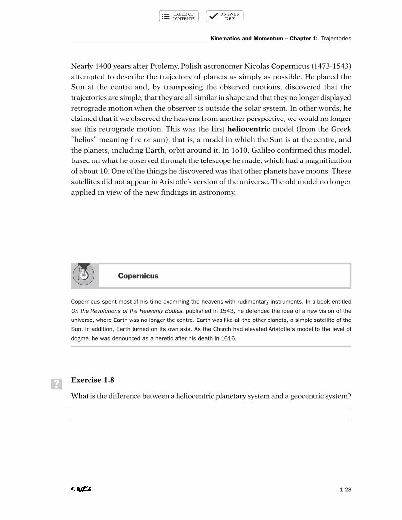
Copernicus spent most of his time examining the heavens with rudimentary instruments. In a book entitled

On the Revolutions of the Heavenly Bodies, published in 1543, he defended the idea of a new vision of the

universe, where Earth was no longer the centre. Earth was like all the other planets, a simple satellite of the

Sun. In addition, Earth turned on its own axis. As the Church had elevated Aristotle’s model to the level of

dogma, he was denounced as a heretic after his death in 1616.

Exercise 1.8

What is the difference between a heliocentric planetary system and a geocentric system?

Copernicus


1.23

?

Exercise 1.9

Figure 1.10 shows the trajectory of Mars as seen by an Earth-based observer. The dotted

lines show the direction from which we see Mars from Earth at different times.

a) Describe the planet’s motion as seen from Earth.

b) How do you explain this?

c) Assuming you are outside the solar system, how would you describe the trajectory

of Mars?

Motion is considered to exist when an object changes position relative to a fixed or

stationary point of reference. The choice of reference point depends on the situation.

In the geocentric model, the Earth serves as the reference point. It is considered

stationary, and the motion of the planets is described relative to the Earth. In the

heliocentric model, the Sun serves as the fixed reference point.

Closer to home, the ground or an object fixed to the ground generally serves as a

reference point. For instance, in the case of a car, truck or bicycle, this could be a tree,

house, telephone pole or fire hydrant.

To clarify concept of reference points, suppose we want to represent the position of

a stationary object in a Cartesian coordinate system. In Figure 1.11, several reference

points can be used to describe the book’s position. As the origin, we can use the southwest

corner of the room at the intersection between the floor and two of the walls

(Figure 1.11a). In this reference system, the book is six metres east, four metres north

and two metres up. In terms of x, y and z coordinates, we could write (6, 4, 2). An

observer looking through the window will choose a different reference system (Figure

1.11b) and the coordinates would then be (–4, 4, 2). The book did not change position

but the coordinates that describe its position vary depending on the reference point.


1.24

?

Figure 1.11 – Locating an object in a room

a) The origin of the reference system is the southwest corner of the room. The coordinates of the book are (6, 4, 2).

b) The origin of the reference system is the southeast corner of the room. The coordinates of the book are (–4, 4, 2).

When stating the position of an object or describing a trajectory, you must specify the

chosen reference system. In practice, however, the reference system is usually not

mentioned when it is the ground, since there is no ambiguity in this case.

Keep in mind that there is no absolute reference system for determining the position

of objects that are stationary or moving. The position of an object is always given relative

to other objects, that is, relative to an arbitrarily chosen reference point. The same

applies to trajectories. As we saw for planetary motion, the trajectory does not

change, but the shape of the path described varies depending on the reference system

selected.

The following figure shows a package being dropped from an airplane. From the pilot’s

viewpoint, the package describes a vertical rectilinear trajectory, since the airplane

continues to move horizontally above the package. Conversely, the observer on the

ground would see the package follow a curved (actually in this case, parabolic) path.

a)Up

West

Down South East x

2

6

4

z

b)Up

North

West

Down South

East x–4

z

2

y

4

North y


1.25

Figure 1.12 – Trajectory in two different reference systems

The airplane moves at a constant velocity, and in its fall, the package continues its horizontalmotion at the same velocity as the airplane. The pilot sees the package decrease in size as it falls

and perceives a vertical rectilinear trajectory. For an observer on the ground, the package follows a curved (parabolic) path resulting from both the airplane’s horizontal motion

and the vertical motion of the falling package.

The description of the trajectory depends on the observer’s frame of reference. The example

above clearly indicates that the trajectory is not absolute, but relative to a reference system.

It is important to specify the reference point in order to eliminate any confusion.

Exercise 1.10

1. A basketball player dribbles the ball on the spot vertically just below his eyes.

a) What does he see? Is this a trajectory? Explain your answer.

b) A spectator in the bleachers sees the player dribbling the ball. Draw the ball’s

trajectory, if the spectator is:

– sitting at the same height as the ball.

– sitting high up in the bleachers.


1.26

?

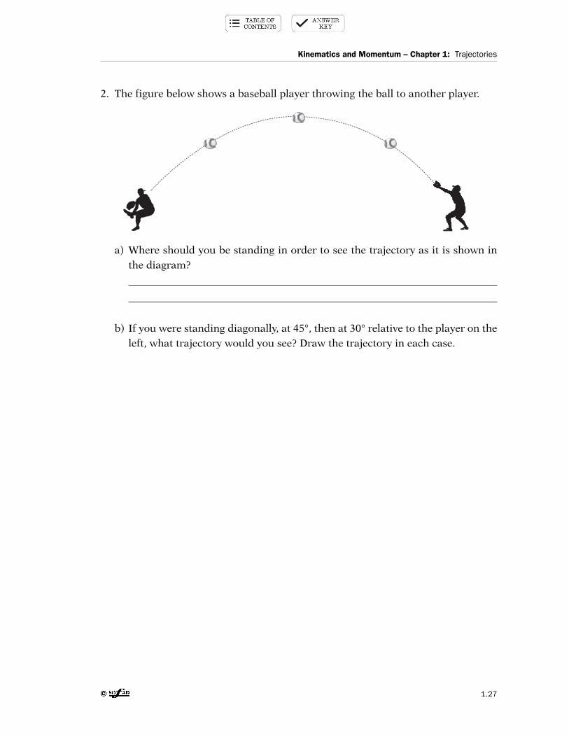
2. The figure below shows a baseball player throwing the ball to another player.

a) Where should you be standing in order to see the trajectory as it is shown in

the diagram?

b) If you were standing diagonally, at 45°, then at 30° relative to the player on the

left, what trajectory would you see? Draw the trajectory in each case.


1.27

c) If you were the one throwing the ball, what trajectory would you see then? Draw

this trajectory.

3. You are an astronaut stationary in space and, through powerful binoculars, you

see a person who is stationary during the period when the Earth is illuminated.

Draw the trajectory that you see for the person, taking into account the fact that

you are not in orbit around Earth.


1.28

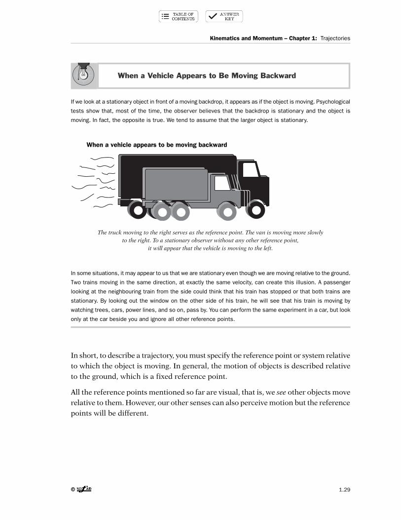
If we look at a stationary object in front of a moving backdrop, it appears as if the object is moving. Psychological

tests show that, most of the time, the observer believes that the backdrop is stationary and the object is

moving. In fact, the opposite is true. We tend to assume that the larger object is stationary.

When a vehicle appears to be moving backward

The truck moving to the right serves as the reference point. The van is moving more slowly to the right. To a stationary observer without any other reference point,

it will appear that the vehicle is moving to the left.

In some situations, it may appear to us that we are stationary even though we are moving relative to the ground.

Two trains moving in the same direction, at exactly the same velocity, can create this illusion. A passenger

looking at the neighbouring train from the side could think that his train has stopped or that both trains are

stationary. By looking out the window on the other side of his train, he will see that his train is moving by

watching trees, cars, power lines, and so on, pass by. You can perform the same experiment in a car, but look

only at the car beside you and ignore all other reference points.

In short, to describe a trajectory, you must specify the reference point or system relative

to which the object is moving. In general, the motion of objects is described relative

to the ground, which is a fixed reference point.

All the reference points mentioned so far are visual, that is, we see other objects move

relative to them. However, our other senses can also perceive motion but the reference

points will be different.

When a Vehicle Appears to Be Moving Backward


1.29

A SENSE OF MOTION

Motion can be detected in several ways: we can see a bird fly, hear the noise of a car

moving away from or toward us, feel a cat brush up against our leg or smell kitchen

aromas wafting through the house. While most of our perceptions of motion are visual,

our other senses—hearing, smell and touch—can also provide information on the

motion of objects. In fact, all of our senses act like probes, which tell us what is

happening in our environment. These probes continually collect information that our

brain interprets, and this is very useful in dangerous situations.

Exercise 1.11

For each of the following situations, identify which sense is most likely to provide

information on the motion described. Explain your answer.

a) You know that an ambulance is approaching your house.

b) Your neighbour is barbecuing hamburgers and you conclude that the wind is coming

from the east.

c) You feel the air that is being blown in your direction by a fan.

d) A cyclist is riding his bicycle.

In the above exercise, your ears tell you that an ambulance is approaching because

the siren becomes increasingly louder. Your nose tells you that an easterly wind is

blowing, which is simply a displacement of air. The smell from the barbecue is due

to the volatile chemicals released by the cooking process and blown by the wind. You

feel the motion of the air generated by the fan on your skin and hair. Lastly, your eyes

see the cyclist riding his bicycle. We can therefore detect motion with our eyes, but

also with our senses of hearing, smell and touch.


1.30

?

In the following pages, we will focus on the perception of motion through our sense

of hearing. Have you ever noticed that the sound of a race car is different when it is

moving toward us than when it is moving away? To understand this phenomenon,

let’s explore the nature and characteristics of sound.

Sounds result from the motion of air, which transmits waves that our ears pick up.

Our ears then convert the waves into signals that our brain recognizes and interprets.

This is how we distinguish between voices, music or simply ambient noises.

Exercise 1.12

An astronaut walking on the Moon throws a stone. Does the stone make a sound upon

hitting the ground? Explain your answer.

Döppler Effect

We can produce sounds with any object which can vibrate, such as a tuning fork8 or

a guitar string. A tuning fork is used to tune musical instruments such as pianos and

guitars. It vibrates when struck with a felt hammer. Each prong then moves back and

forth rapidly and this displaces the air around the prongs. The resulting vibration creates

alternating compressions (areas where the air is denser) and rarefactions (areas where

the air is thinner) (Figure 1.13).


1.31

?

8. A tuning fork is a small, steel, two-pronged instrument which produces a specific musical note when made tovibrate.

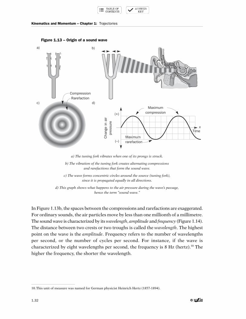
Figure 1.13 – Origin of a sound wave

a) The tuning fork vibrates when one of its prongs is struck.

b) The vibration of the tuning fork creates alternating compressions and rarefactions that form the sound wave.

c) The wave forms concentric circles around the source (tuning fork), since it is propagated equally in all directions.

d) This graph shows what happens to the air pressure during the wave’s passage, hence the term “sound wave.”

In Figure 1.13b, the spaces between the compressions and rarefactions are exaggerated.

For ordinary sounds, the air particles move by less than one millionth of a millimetre.

The sound wave is characterized by its wavelength, amplitude and frequency (Figure 1.14).

The distance between two crests or two troughs is called the wavelength. The highest

point on the wave is the amplitude. Frequency refers to the number of wavelengths

per second, or the number of cycles per second. For instance, if the wave is

characterized by eight wavelengths per second, the frequency is 8 Hz (hertz).10 The

higher the frequency, the shorter the wavelength.

Maximumrarefaction

Maximumcompression

Cha

nge

in a

irpr

essu

re

a) b)

c) d)

(+)

Time x

(–)

CompressionRarefaction


1.32

10.This unit of measure was named for German physicist Heinrich Hertz (1857-1894).

Figure 1.14 – Characteristics of sound waves

a) Amplitude and wavelength.

b) High-pitched sound has a high frequency; low-pitched sound has a low frequency.

c) A sound is as loud when the wave’s amplitude is large.

The amplitude of the wave determines whether the sound is loud (large amplitude)

or soft (small amplitude), while the frequency determines whether the sound has a

low pitch (low frequency) or a high pitch (high frequency).

Amplitude

a)

(+)

Time

Time

x

x

Timex

(–)

Wavelength

b)(+)

(–)

High-pitched sound: highfrequency and short wavelength

Low-pitched sound: lowfrequency and long wavelength

Loud sound: large amplitude Soft sound: small amplitude

c)(+)

(–)


1.33

Exercise 1.13

a)

This figure represents a scale of a piano. The notes are played on the white keys.

Which key produces the sound with the highest pitch? The lowest? Explain your

answer.

b)

The above figure represents sound waves. Which diagram shows the sound with

the highest pitch? Explain your answer.

Time

Time

Air p

ress

ure

(+)

A

(–)

Air p

ress

ure

(+)

B

(–)

Note do re mi fa so la ti do

Frequency 262 294 330 349 392 440 494 524


1.34

?

The human ear is sensitive to sound waves with frequencies of between 20 and 20 000 hertz. Frequencies

lower than 20 hertz are infrasounds and those with frequencies higher than 20 000 hertz are ultrasounds.

Infrasounds and ultrasounds are waves similar to sound waves, except that they are inaudible by humans.

Underground nuclear explosions, tides and earthquakes produce infrasounds and are detected by a

seismograph.

Many animals produce and hear ultrasounds. For instance, humans hear only a portion of the sounds made

by a mouse, whereas cats can hear the ultrasonic sounds. Bats emit ultrasounds and can detect the presence

of obstacles and prey by listening to the reflection of the waves they emit. This enables them to hunt at night.

Echoes and thunder

Echoes are produced when sound waves are reflected by walls or mountains. However, no echo is possible if

the reflected wave reaches the ear less than 1/10 of a second after the original sound was produced. As the

ear cannot distinguish between the two sounds (the original sound and the echo), we call this a reverberation.

Since sound travels at about 330 m/s, the reflecting surface must be at least 16.5 metres away for an observer

to hear the echo.

Echo

Wall

Source

Infrasounds and Ultrasounds


1.35

Sonar

Sonar11 is a device used on boats to determine distances. It functions like radar, except that sonar uses sound

waves instead of radio signals. A transmitter underneath the boat generates sound waves that travel through

the water and bounce off submerged objects or the bottom. The reflected waves are picked up by a receiver,

which is also underneath the boat. Sonar provides information on the distance between the boat and the objects

reflecting the sound waves by measuring the time interval between the moment the sound waves are emitted

and the moment they are received.

Now that we know a bit more about the nature of sound and the way it travels, let’s

return to the perception of motion by means of sound. Two different factors need to

be considered. The first is the sound’s amplitude. For instance, we know that a car is

moving away from us when it becomes less audible. Conversely, the amplitude of sound

increases if the car is moving toward us.

The second factor is the sound frequency. Assume that you are standing at an

intersection and a fire truck approaches and then passes you. You probably notice

that the sound of the siren is not the same before and after the fire truck passes. In

reality, the sound frequency you hear is higher when the fire truck is approaching than

when it is moving away. Why is this, when the frequency of the siren itself does not

change? Let’s examine this further.

Pêches et Océans Canada

ReceiverTransmitter

Sound wavesemitted

Sound wavesreflected


1.36

11. SONAR is the acronym for Sound Navigation and Ranging.

Figure 1.15a) shows a stationary fire truck, with its siren on. Notice how the sound

waves are distributed around the vehicle. The siren always emits sound of the same

frequency. However, when the van is moving (Figure 1.15b), the waves in front of the

truck become more compact. We could say that the truck is chasing its sound waves.

Thus, a stationary observer will perceive more waves per second when the truck is

moving toward him. The sound will have a higher frequency than that generated by

the stationary siren, in other words, a sound with a higher pitch (Figure 1.15b).

Conversely, when the fire truck moves away, the sound waves disperse behind the truck

as though the truck were fleeing the sound waves. The sound then has a lower frequency,

that is, a lower sound than that produced by the stationary siren (Figure 1.15c). This

phenomenon is called the Döppler effect, named after Christian Döppler, who

discovered it.12

Figure 1.15 – Sound and the Döppler effect

a) Both observers hear the sound at the frequency emitted by the siren.

b) The observer toward whom the fire truck is moving hears a sound that is higher-pitched than when the truck was stationary. Conversely, the observer on the left hears

a lower-pitched sound than that produced by the stationary siren.

c) If the fire truck moves faster, the observer on the right will hear a sound with a still higher pitch.The observer on the left will hear a lower-pitched sound than in b).

a) Stationary fire truck

b) Moving fire truck

c) Fire truck moving faster


1.37

12.There are many interactive applets on the Internet that illustrate the Döppler effect. They made be found by entering“Döppler effect applet” in a search engine. One example may be found at www.phy.ntnu.tw/java/Doppler/Doppler.html.

Exercise 1.14

1. The figure below shows the waves emitted by an ambulance siren.

a) In what direction is the ambulance moving? Explain your answer.

b) Which observer will hear a sound with a higher pitch than that generated by

the siren? State why.

c) Will the other observer hear a sound with a lower pitch than that generated by

the siren? State why.

The Döppler effect also applies in the reverse, that is, when the sound source is stationary

and the observer is moving. The frequency perceived by the observer is then higher

or lower, depending on whether he is approaching or moving away from the source.

Let’s use the example of a train approaching, then moving away from a stationary siren.


1.38

?

Figure 1.16 – Döppler effect in the case of a stationary sound source

a) The train approaches the siren. It therefore encounters more sound waves per second than when it was stationary; the frequency received is higher than that emitted

by the siren and the sound becomes higher pitched.

b) The train moves away from the siren. The train encounters fewer sound waves per second than when it was stationary because it is moving away from the sound source;

the frequency is lower and the sound has a lower pitch.

Döppler’s discovery was extended to light in 1848 by French physicist Hippolyte Fizeau.

He suggested that what is true for sound also applied to light. The light emitted by a

star or galaxy moving away from us is perceived at a lower frequency than that emitted

by the Sun. Conversely, a galaxy or a star emits light at a slightly higher frequency

when it moves toward us. In the spectrum of visible light, red corresponds to the lower

frequencies (longer wavelengths) and blue and violet to the higher frequencies

(shorter wavelengths) (Figure 1.17a). We will therefore see a red shift for a star moving

away from us and a blue shift for a star approaching us.

But how do we know the frequency at which the light of a star is emitted at the outset,

and what tells us that it has undergone a shift? These are valid questions. The gases

contained in the stars provide the answer. Consider hydrogen.

Scientists analyze the light of the stars using a spectrograph, which separates the

wavelengths (or frequencies) received. The galaxies contain billions of stars, and

hydrogen is their main fuel. Each gas, when excited, gives off a few specific wavelenghts

of light. This is its characteristic spectrum or its signature. Hydrogen’s spectrum consists

of four wavelengths of visible light, called spectral lines, whose values are 410.2 nm,

434.0 nm, 486.1 nm and 656.3 nm (Figure 1.17b).13

a) b)


1.39

13. 1 nm = 1 nanometer = 1 × 10–9 m. These wavelengths are very short.

Figure 1.17 – The Döppler effect applied to light

a) The visible spectrum comprises all the wavelengths between 400 nm (violet) and 700 nm (red).

b) When excited, hydrogen is characterized by four specific visible light wavelengths. Together, these four lines form hydrogen’s spectrum. They can be considered hydrogen’s fingerprint.

c) When a galaxy moves away from Earth, the lines display a red shift (to the right on the diagram). The wavelength of each line increases, that is, its frequency decreases.

The amount of red shift makes it possible to determine precisely the receding velocity of a star or galaxy.

d) When a star or galaxy approaches Earth, the lines display a blue shift (to the left on the diagram). Their wavelength decreases, that is, their frequency increases.

a)

b)

infrared

redyellow

green

violetblue

ultraviolet

800 n

m

700 n

m

600 n

m

500 n

m

400 n

m

300 n

m

200 n

m

656,3

nm

486,1

nm

434,0

nm

410,2

nm

red blue

red blue

red blue

c)Earth

Earth

Galaxy

d)

Galaxy


1.40

When a spectrograph indicates a star’s spectrum, hydrogen’s signature is visible, in

other words, its four spectral lines are always present. In 1920, while studying remote

galaxies, Edwin Hubble (1889-1953) discovered that the spectral lines of hydrogen

had slightly longer wavelengths than those emitted by hydrogen in the laboratory. He

observed 411.54 nm, 435.50 nm, 487.75 nm and 658.47 nm. Each line showed a shift

of 0.0033% relative to the known value. Hubble deduced that the red shift was due to

the Döppler effect. Thus, when a galaxy moves away from us, we perceive a lower

frequency (a longer wavelength) than that emitted by the source. This is similar to

what happens to the sound you hear when an ambulance moves away from you.

Hubble’s calculations showed that certain galaxies were moving away from the Earth

at a speed of 1 000 000 m/s, and thus he proved that the universe was expanding.

Furthermore, distant galaxies are moving away from us at even greater speeds than

the nearby ones. Certain galaxies located ten billion light-years away travel at 90% of

the speed of light, or 270 000 km/s.

Exercise 1.15

Most galaxies are moving away from us, but not the Andromeda galaxy, located at a

distance of 2.2 light-years from the Milky Way, which is moving toward us at 50 km/s.

Will the light’s wavelengths exhibit a blue shift or a red shift? Explain your answer.

Applied to light, the Döppler effect allows us to determine the speed at which the stars

and galaxies are moving toward or away from us. Through this phenomenon,

astrophysicists have learned more about the motion of celestial bodies and concluded

that our universe is expanding. In fact, a red shift is observed for the vast majority of

celestial bodies because they are moving away from us.


1.41

?

The topic of motion, simple at first glance, has given rise to a great deal of discussion

in this chapter. We explored the concept of trajectory and the different types of

trajectories; Aristotle’s theories on motion and the trajectories of planets, and the

debunking of these theories by Galileo; and Newton’s explanation of how objects

fall and how planets move. We also examined a wide range of topics encompassed

by mechanics, which is the study of motion and is subdivided into a number of

branches. This chapter also discussed the importance of the observer’s reference

point in the description of a trajectory, and the role of our senses—particularly

sight and hearing—in the perception of motion. The concept of trajectory served

as a backdrop to the diverse content of this chapter. The next chapter examines

the distance covered by an object along a trajectory and the resulting displacement

between the start and finish points.


1.42

Amplitude

Circular trajectory Classical mechanicsCurvilinear trajectory

Döppler effect Dynamics

Elliptical trajectory

Fluid mechanics Frequency

Kinematics

Parabolic trajectory

Quantum mechanics

Rectilinear motion Rectilinear trajectoryReference point Relativistic mechanicsRetrograde motion

Sound wave

Thermodynamics

Wavelength

The history of motion begins with Aristotle. His theories endured for thousands of

years, until Galileo and Newton proved them wrong.

Aristotle theorized that objects in motion seek to return to their natural place, that

is, to remain at rest. Galileo and Newton believed that an object tends to maintain its

state of motion, provided it is not affected by any external forces.

The introduction of the concept of force was crucial. In fact, it explains why a moving

object can eventually stop because of friction, for instance. The concept of force explains

this phenomenon, while the concept of an object’s natural place explains nothing.

SUMMARY

KEY WORDS IN THIS CHAPTER


1.43

Aristotle’s and Ptolemy’s models of the universe are geocentric, whereas Galileo’s and

Newton’s are heliocentric. Galileo’s invention of the telescope made it possible to prove

conclusively that our planetary system is heliocentric.

While Aristotle claimed that a heavy object reached the ground before a light one when

released at the same time, Galileo’s experiment proved otherwise.

An object is in motion when it changes position relative to a fixed reference point.The choice of reference point is arbitrary, since there is no absolute reference point,

that is, one that can be used to explain all motion. As a result, there is no absolute

motion either.

We describe motion through the concept of trajectory. All successive points (imaginary)

occupied by the moving object constitute its trajectory. Trajectories can be rectilinear,curvilinear (elliptical, circular, parabolic) and random. Since the trajectory

described always depends on the observer’s viewpoint, we must be careful when

describing one.

If sight is crucial for describing the trajectory of a moving object, hearing is also

important for determining if a sound source is moving toward or away from us.

Döppler’s research has shown that when a sound source is approaching, the sound

becomes increasingly higher in pitch due to the increased frequency of the sound

waves. When the source moves away, the frequency of the sound waves decreases and

the sound becomes lower in pitch.

Sound waves are produced by alternating compressions and rarefactions of air

around the sound source. They disperse in a spherical three-dimensional space. The

change in the air pressure around a sound source is described by a sine curve. The

sine curve does not represent the sound wave in the air, it is only a graphical

representation of the change in air pressure as a function of time. This phenomenon

is explained by the vibration of the sound source.

The next chapter will deal with displacement, that is, the change in position of an object

relative to a fixed reference point. You will learn that displacement has two

characteristics: magnitude and direction.


1.44

Exercise 1.16

The first known theories on motion have been attributed to Aristotle. About 2000 years

later, Galileo and Newton proved that these theories were incorrect.

a) What distinguishes Aristotle’s general theory of objects in motion from that of

Newton?

b) What distinguishes Aristotle’s theory of objects in free fall from that of Galileo?

c) What is the main difference between Aristotle’s and Galileo’s model of the universe?

REVIEW EXERCISES


1.45

?

Exercise 1.17

A passenger train is moving along a rectilinear trajectory. Draw the trajectory of the

motion of a seated passenger you see through the window of the train if:

Note: Close your eyes and imagine that the passenger is represented by a point.

a) you are stationary;

b) you are moving at the same velocity and in the same direction as the train.

Exercise 1.18

You notice a safety reflector (a plastic object generally red in colour, which reflects

light) mounted on the spoke of a bicycle wheel that is moving in a straight line to the

left at a constant speed. Draw the trajectory of this reflector as you observe it when

you are:

a) stationary and to one side of the bicycle;

b) on another bicycle moving parallel to the reflector and at the same velocity.


1.46

?

?

Exercise 1.19

The figure below shows a sound wave and the corresponding sine curve.

a) Identify the compressions and rarefactions by the appropriate letter.

b) Does the graph represent a sound wave? Explain your answer.

c) How does sound travel in the air?

Exercise 1.20

The figure below is a locomotive blowing its horn.

a) Which observer will hear the higher-pitched sound? Explain.

b) Which observer will hear a sound with a higher frequency?

A B

patm

pmax

pmax

Air p

ress

ure

Time

A B C D


1.47

?

?

Exercise 1.21

Examine the figure below. At which point will the child hear a high-pitched sound?

Why?

Exercise 1.22

The figure below shows a swinging pendulum as seen from positions A, B and C. Draw

the trajectory of the pendulum perceived from these positions.

A : B : C :

A Front view

B

C

Whistle

A B C D E


1.48

?

?

Exercise 1.23

1. Imagine you are at the top of a ten-storey building, your head is out the window,

and you drop a black ball. A passerby stops to watch.

a) Describe the trajectory as seen by the passerby.

b) What do you see from the window?

c) Is what you see in b) a trajectory? Explain.


1.49

?

Documents

Kinematics and Momentum - SOFAD · The first learning guide is complemented by the workbook entitled ... commissions scolaires du Québec ... Collisions in Which Objects Remain Stuck