Embed Size (px)
Citation preview

KINETIC MODEL OF DNA REPLICATION AND
THE LOOPING OF SEMIFLEXIBLE POLYMERS
by
Suckjoon JUN
BSc., Busan National University, Busan, Korea, 1997
MSc., Iowa State University, Ames, IA, USA, 1999
THESIS SUBMITTED IN PARTIAL FULFILLMENT
OF THE REQUIREMENTS FOR THE DEGREE OF
DOCTOR OF PHILOSOPHY
IN THE DEPARTMENT
OF
PHYSICS
c© Suckjoon JUN 2004
SIMON FRASER UNIVERSITY
July, 2004
All rights reserved. This work may not bereproduced in whole or in part, by photocopy
or other means, without permission of the author.

ii
APPROVAL
Name: Suckjoon JUN
Degree: Doctor of Philosophy
Title of Thesis: Kinetic Model of DNA Replication andthe Looping of Semiflexible Polymers
Examining Committee:
Chair: Dr. Barbara FriskenProfessor of Physics
____________________________________
Dr. John BechhoeferSenior SupervisorProfessor of Physics
____________________________________
Dr. Michael WortisSupervisorProfessor Emeritus of Physics
____________________________________
Dr. Martin ZuckermannSupervisorAdjunct Professor of Physics
_______________________________________
Dr. Dipankar SenSupervisorProfessor of Molecular Biology and Biochemistry
_______________________________________
Dr. Peter J. UnrauInternal ExaminerAssistant Professor ofMolecular Biology and Biochemistry
_______________________________________
Dr. William M. GelbartExternal ExaminerProfessor of Chemistry and BiochemistryUniversity of California, Los Angeles
Date Approved: July 15, 2004

Abstract
Biological systems are a rich source of new problems in physics, and solving them requires ideas
from various fields. In this thesis, we focus on the specific biological phenomenon of DNA replica-
tion, which is tightly regulated by spatio-temporal “programs” during the cell cycle.
Inspired by a formal analogy between DNA replication and one-dimensional nucleation-and-
growth processes, we extend the 1D Kolmogorov-Johnson-Mehl-Avrami (KJMA) model to arbitrary
nucleation ratesI(t). We then use the KJMA model to extract kinetic parameters from data taken
from molecular combing experiments. The analysis developed here can help biologists to understand
and compare temporal programs of DNA replication of different organisms from a unified scheme.
After developing the kinetic model, we show how underlying physical properties of chromatin,
in particular its intrinsic stiffness, can explain various long-standing experimental observations.
These include synchrony and correlations in the initiation of replication origins, as well as deter-
mination of the origin spacings in the absence of sequence requirements in early embryos.
iii

Γ ια σενα
iv

Acknowledgments
Before one hears his vocation, he is a man; IFF my soul has any decencies, it is the unconditional
love from my parents, my little brother, and my late grandparents that I am indebted for. It always
has been. And it always shall be.
I grew up in a culture where one’s teachers are regarded as his extended parents. If I would
be considered as a good and honest scientist one day, it must be that I was once a student of John
Bechhoefer. Through him, I have started to learn how to read, write, speak, and think. Back in 2000,
it must not have been easy for John to take me as his student, but I would choose him as a thesis
advisor – my intellectual father – again.
I am fortunate to have had several other mentors and friends during my “vagabond” career
in graduate school: I am deeply grateful to Aaron Bensimon for his constant encouragement and
having faith in my research, who called me his friend despite the gap in our ages, experiences, and
intellects. I also would like to thank John Herrick for helping me learn biology and also showing
me there are different kinds of lives out there. And from Bae-Yeun Ha, I have learned not only the
beauty of physics and physics itself, but also kindness and patience that any man should have. I owe
these people more than words can say.
Coming from physics, learning biology was a series of surprises, frustrations, and joys. During
this course of discovering “my ignorance, my desires, my willingness,” interactions with the follow-
ing biologists have been particularly and truly inspiring: Geneviève Almouzni, Benoit Arcangiolo,
Ellen Fanning, Joel Huberman, and Philippe Pasero. Equally memorable, my meeting with Mark
Goulian, Stan Leibler, and Peter Unrau made me realize why I do what I do.
Looking back, I realize it has been a great privilege to study biophysics at Simon Fraser. Just
being surrounded by and interacting with the following professors made me feel I belong to a special
group of people: John, Dave Boal, Barbara Frisken, Mike Plischke, Dipankar Sen, Jenifer Thewalt,
Michael Wortis, and Martin Zuckermann; and (former) graduate students and post-docs: Bae-Yeun,
v

ACKNOWLEDGMENTS vi
Michale Dugale, Martin Howard, Gerald Lim, Anirban Sain, Vahid Shahrezaei, and Dan Vernon.
In the last four years, in addition to my long-term collaborators Aaron, John, and Bae-Yeun,
I have enjoyed collaborations and discussions with the following people: Ken Sekimoto on the
KJMA model; Jeff Chen, Binny Cherayil, Arti Dua, Mohammed Kohandel, Christophe Koudella,
Alexei Podtelezhnikov, Dipankar Sen, and Michael Wortis on loop formation of semiflexible poly-
mers; Pu Chen, Yooseong Hong, Hideo Immamura, and Christophe Koudella on self-assembly of
charged peptides; Tom Chou on various statistical mechanics and biophysics problems; Julian J.
Blow, Bernie Dunker, Olivier Hyrien, Nick Rhind, and the biologists mentioned above on DNA
replication. During this period, I have travelled many places and, particularly, would like to thank
Ellen (Vanderbilt University, Nashville), Bae-Yeun and Pu (Univ. of Waterloo, Waterloo), and Bela
Mulder (AMOLF, Amsterdam) for their hospitalities during my visit.
While working on this thesis, the following people have kindly helped me: Ron Berezney and
Kishore Malyavantham with the replication foci image; Gary Felsenfeld and Mark Groudine with
the illustration of higher-order structure of chromatin from their Nature article; Jeni Koumoutsakis
and her mother with Greek.
I have always thought that I have very few friends. How wrong I was, because I have this many
friends to thank for their invaluable friendships: my Korean connections – Yonghyun from my
childhood, Kyungchor (we discussed from Hilbert to Wittgenstein), Yunhee, and the “mathmanias”
Eunjin, Hyejoeng, Hyojin, Hyunjeong, Jina, Songhee, Woonjung, Youngsoon from university; the
Iranian connections – Babak, Kamran, Simin, Vahid; people from the Bechhoefer lab – Bram-
Marnie-Nadav, Haiyang, Phil, Yuekan, and visitors to our lab Mélanie, Peter, Russ, Sébastien; the
“panini” connection – Bruna and Columba; the ladies in the physics department – Candida, Dagni,
Helen, Sue; my special friend from the Boulder summer school Ginestra; my cinephile friends Chan
and Stan; (thanks, Stan, for always being there when I am lost, and, Heather, I will remember our
short walk in the “wheatfield” for a long time); friends from SFU – Cecilia, Gerald, Karl, Karn,
Matt, Patricia, Philippe; from Waterloo – Andy, Hideo, Yooseong; from Iowa State University –
Bassam, Dave, Julie; and the staffs at Early Music Vancouver and Pacific Cinémathèque.
I also would like to thank my former teachers, especially, Profs. Seyoung Jeong and Hyuk-Kyu
Pak at Busan National University in Korea, and Marshall Luban and Constantin Stassis at Iowa State
University in Ames, IA.
I cannot finish my acknowledgments without mentioning my experiences in Aaron’s lab at Insti-
tut Pasteur and life in Paris back in 2001. My nostalgia for the people, the life, and even the stupid

ACKNOWLEDGMENTS vii
mistakes I made in those six months is as strong as for my entire childhood: Aaron and his family
for embracing me; Catherine, Chiara, Fabrice, Hélène and Nicolas, Katya, Reiner, and Sandrine for
their friendships and help for my survival; Benoit, Bianca, John for countless number of beers and
discussions from philosophy to films at Pouchla and other cafes.
And finally, I would like to acknowledge my infinite source of inspirations, J. S. Bach.
EPILOGUE: Knowing the influences on shaping my humble being by all these people, how could I
not think of words of my hero François Jacob?
And then, how not to see that all these selves of my past life have played the greatest
role, and the greater the earlier they came, in the development of the secret image
that from the deepest part of me guides my tastes, desires, decision. Starting in the
younger years, imagination seizes on the people and things it encounters. It grinds
them down, transforms them, abstracts a feature or a sign with which to shape our
ideal representation of the world. A schema that becomes our system of reference, our
code to decipher oncoming reality. Thus, I carry within a kind of inner statue, a statue
sculpted since childhood, that gives my life a continuity and is the most intimate part
of me, the hardest kernel of my character. I have been shaping this statue all my life. I
have been constantly retouching, polishing, refining it. Here, the chisel and the gouge
are made of encounters and interactions; of discordant rhythms; of stray pages from one
chapter that slip into another in the almanac of the emotions; terrors induced by what is
all sweetness; a need for infinity erupting in bursts of music; a delight surging up at the
sight of a stern gaze; an exaltation born from an association of words; all the sensations
and constraints, marks left by some people and by others, by the reality of life and by
the dream. Thus, I harbor not just one ideal person with whom I continually compare
myself. I carry a whole train of moral figures, with utterly contradictory qualities,
who in my imagination are always ready to act as my fellow players in situations and
dialogues imprinted in my head since childhood or adolescence. For every role in this
repertory of the possible, for all the activities that surround me and involve me directly,
I thus hold actors ready to respond to cues in comedies and tragedies inscribed in me
long ago. Not a gesture, not a word, but has been imposed by the statue within.1
1François Jacob,The Statue Within, Basic Books, New York, 1988.

Contents
Approval ii
Abstract iii
Dedication iv
Acknowledgments v
Contents viii
List of Tables xi
List of Figures xii
1 Introduction 1
1.1 Physics and biology united: a brief overview . . . . . . . . . . . . . . . . . . . . . 1
1.2 Getting started: a brief history of DNA replication . . . . . . . . . . . . . . . . . . 3
1.3 About this thesis . . . . . . . . . . . . . . . . . . . . . . . . . . . . . . . . . . . 10
2 Generalized KJMA Model 12
2.1 Introduction . . . . . . . . . . . . . . . . . . . . . . . . . . . . . . . . . . . . . . 12
2.2 Theory . . . . . . . . . . . . . . . . . . . . . . . . . . . . . . . . . . . . . . . . . 17
2.2.1 Island fractionf(t) . . . . . . . . . . . . . . . . . . . . . . . . . . . . . . 17
2.2.2 Hole-size distributionρh(x, t) . . . . . . . . . . . . . . . . . . . . . . . . 18
2.2.3 Island distributionρi(x, t) . . . . . . . . . . . . . . . . . . . . . . . . . . 20
2.2.4 Island-to-island distributionρi2i(x, t) . . . . . . . . . . . . . . . . . . . . 22
viii

CONTENTS ix
2.3 Numerical simulation . . . . . . . . . . . . . . . . . . . . . . . . . . . . . . . . . 26
2.4 Comparison between theory and simulation . . . . . . . . . . . . . . . . . . . . . 29
2.5 Conclusion . . . . . . . . . . . . . . . . . . . . . . . . . . . . . . . . . . . . . . 31
3 Application to DNA Replication Kinetics 32
3.1 Introduction . . . . . . . . . . . . . . . . . . . . . . . . . . . . . . . . . . . . . . 32
3.2 Application of the 1D-KJMA Model to Experimental Systems . . . . . . . . . . . 33
3.2.1 Ideal case . . . . . . . . . . . . . . . . . . . . . . . . . . . . . . . . . . . 34
3.2.2 Asynchrony . . . . . . . . . . . . . . . . . . . . . . . . . . . . . . . . . . 36
3.2.3 Finite-size effects . . . . . . . . . . . . . . . . . . . . . . . . . . . . . . . 40
3.2.4 Finite-resolution effect . . . . . . . . . . . . . . . . . . . . . . . . . . . . 43
3.3 Discussion and Conclusion . . . . . . . . . . . . . . . . . . . . . . . . . . . . . . 44
4 Temporal Program of XenopusDNA Replication 46
4.1 Introduction . . . . . . . . . . . . . . . . . . . . . . . . . . . . . . . . . . . . . . 46
4.2 Results . . . . . . . . . . . . . . . . . . . . . . . . . . . . . . . . . . . . . . . . . 48
4.2.1 Summary of theXenopusegg extracts replication experiment . . . . . . . . 49
4.2.2 Generalization of the model to account for specific features of theX. laevis
experiment . . . . . . . . . . . . . . . . . . . . . . . . . . . . . . . . . . 51
4.2.3 Application of the kinetic model to the analysis of DNA replication inX.
Laevis . . . . . . . . . . . . . . . . . . . . . . . . . . . . . . . . . . . . . 52
4.3 Discussion . . . . . . . . . . . . . . . . . . . . . . . . . . . . . . . . . . . . . . . 57
4.3.1 Initiation throughout S phase . . . . . . . . . . . . . . . . . . . . . . . . . 57
4.3.2 Asynchrony, finite-size, and finite-resolution effects . . . . . . . . . . . . . 57
4.3.3 Directions for future experiments inX. laevis . . . . . . . . . . . . . . . . 58
4.3.4 Applications to other systems . . . . . . . . . . . . . . . . . . . . . . . . 59
4.3.5 The random-completion problem: part I . . . . . . . . . . . . . . . . . . . 59
4.4 Conclusion . . . . . . . . . . . . . . . . . . . . . . . . . . . . . . . . . . . . . . 62
4.5 Appendix . . . . . . . . . . . . . . . . . . . . . . . . . . . . . . . . . . . . . . . 63
4.5.1 Monte Carlo simulations . . . . . . . . . . . . . . . . . . . . . . . . . . . 63
4.5.2 Parameter extraction from data and experimental limitations . . . . . . . . 64

CONTENTS x
5 Spatial Program ofXenopusDNA Replication 66
5.1 Introduction . . . . . . . . . . . . . . . . . . . . . . . . . . . . . . . . . . . . . . 66
5.2 Results . . . . . . . . . . . . . . . . . . . . . . . . . . . . . . . . . . . . . . . . . 69
5.2.1 The eye-to-eye distribution predicted using random initiation does not agree
with experiment. . . . . . . . . . . . . . . . . . . . . . . . . . . . . . . . 70
5.2.2 Eye-size correlations and origin synchrony. . . . . . . . . . . . . . . . . . 72
5.2.3 Origin spacing, loops, and replication factories. . . . . . . . . . . . . . . . 72
5.3 Discussion . . . . . . . . . . . . . . . . . . . . . . . . . . . . . . . . . . . . . . . 76
5.3.1 Persistence length . . . . . . . . . . . . . . . . . . . . . . . . . . . . . . . 76
5.3.2 The random-completion problem: part II . . . . . . . . . . . . . . . . . . 77
5.3.3 Chromatin loops and replication kinetics. . . . . . . . . . . . . . . . . . . 78
5.3.4 Loop formation and replication factories. . . . . . . . . . . . . . . . . . . 79
5.4 Conclusion . . . . . . . . . . . . . . . . . . . . . . . . . . . . . . . . . . . . . . 80
6 Looping of Semiflexible Polymers 82
6.1 Introduction . . . . . . . . . . . . . . . . . . . . . . . . . . . . . . . . . . . . . . 82
6.2 Theoretical Approaches to Modeling Polymers . . . . . . . . . . . . . . . . . . . 86
6.3 Relaxation of a Stiff Chain . . . . . . . . . . . . . . . . . . . . . . . . . . . . . . 89
6.4 Looping Dynamics . . . . . . . . . . . . . . . . . . . . . . . . . . . . . . . . . . 91
6.5 Appendix . . . . . . . . . . . . . . . . . . . . . . . . . . . . . . . . . . . . . . . 102
6.5.1 Review of the Kramers problem . . . . . . . . . . . . . . . . . . . . . . . 102
6.5.2 Reaction-radius dependence and compact vs. non-compact exploration . . 106
7 Conclusion 109
Bibliography 112

List of Tables
3.1 Asynchrony: input vs. extracted parameters . . . . . . . . . . . . . . . . . . . . . 39
4.1 Asynchrony, finite-size, and finite-resolution effects . . . . . . . . . . . . . . . . . 58
xi
List of Figures
1.1 Double-helix structure of DNA . . . . . . . . . . . . . . . . . . . . . . . . . . . . 3
1.2 Schematic model of replication fork . . . . . . . . . . . . . . . . . . . . . . . . . 5
1.3 Eukaryotic cell cycle . . . . . . . . . . . . . . . . . . . . . . . . . . . . . . . . . 6
1.4 Higher-order structure of chromatin . . . . . . . . . . . . . . . . . . . . . . . . . 7
1.5 Electron micrograph showing multiple replication bubbles . . . . . . . . . . . . . 8
1.6 Replication foci and chromatin loops . . . . . . . . . . . . . . . . . . . . . . . . . 9
2.1 Mapping DNA replication onto the one-dimensional KJMA model. . . . . . . . . . 14
2.2 Schematic description of the double-labeling experiment . . . . . . . . . . . . . . 15
2.3 A fluorescence micrograph . . . . . . . . . . . . . . . . . . . . . . . . . . . . . . 16
2.4 Kolmogorov’s method. . . . . . . . . . . . . . . . . . . . . . . . . . . . . . . . . 17
2.5 Illustration for evolution ofρh(x, t) . . . . . . . . . . . . . . . . . . . . . . . . . 18
2.6 Spacetime diagram . . . . . . . . . . . . . . . . . . . . . . . . . . . . . . . . . . 19
2.7 Plot ofs∗(t) . . . . . . . . . . . . . . . . . . . . . . . . . . . . . . . . . . . . . . 23
2.8 Constraint planeS : (i1 + i2)/2 + h = x. . . . . . . . . . . . . . . . . . . . . . . 24
2.9 Simulation algorithm . . . . . . . . . . . . . . . . . . . . . . . . . . . . . . . . . 25
2.10 Simulation times for two algorithms. . . . . . . . . . . . . . . . . . . . . . . . . . 27
2.11 Theory vs. simulation . . . . . . . . . . . . . . . . . . . . . . . . . . . . . . . . . 28
2.12 Decay constants . . . . . . . . . . . . . . . . . . . . . . . . . . . . . . . . . . . . 30
3.1 Parameter extraction from an almost ideal data set . . . . . . . . . . . . . . . . . . 36
3.2 Inversion results in the presence of asynchrony and finite-size effects . . . . . . . . 38
3.3 Rescaled graphs for finite-size effects . . . . . . . . . . . . . . . . . . . . . . . . 41
3.4 The finite-size effects and changes in the basic time and length scales . . . . . . . 42
xii
LIST OF FIGURES xiii
3.5 The effect of coarse-graining . . . . . . . . . . . . . . . . . . . . . . . . . . . . . 43
4.1 Schematic representation of labeled and combed DNA molecules . . . . . . . . . . 50
4.2 ρ(f, τi) distributions for the six time points . . . . . . . . . . . . . . . . . . . . . 53
4.3 Mean quantities vs. replication fraction . . . . . . . . . . . . . . . . . . . . . . . 54
4.4 Extractedf(t) andI(t) . . . . . . . . . . . . . . . . . . . . . . . . . . . . . . . . 55
4.5 Starting-time distributionφ(τ) . . . . . . . . . . . . . . . . . . . . . . . . . . . . 56
4.6 Licensing and activation of replication origins . . . . . . . . . . . . . . . . . . . . 60
4.7 Histogram of positions of initiation events in holes . . . . . . . . . . . . . . . . . 61
4.8 Size-distribution of combed DNA molecules . . . . . . . . . . . . . . . . . . . . . 63
5.1 Random-completion problem and two suggested solutions . . . . . . . . . . . . . 67
5.2 Replication factory and chromatin loops . . . . . . . . . . . . . . . . . . . . . . . 68
5.3 Distribution of replication origins and the loop-formation probability . . . . . . . . 71
5.4 Eye-size correlation . . . . . . . . . . . . . . . . . . . . . . . . . . . . . . . . . . 73
5.5 Computer simulation rules . . . . . . . . . . . . . . . . . . . . . . . . . . . . . . 74
6.1 Schematic description of polymer looping . . . . . . . . . . . . . . . . . . . . . . 84
6.2 Discrete models of polymer . . . . . . . . . . . . . . . . . . . . . . . . . . . . . . 85
6.3 Loop-size distribution . . . . . . . . . . . . . . . . . . . . . . . . . . . . . . . . . 89
6.4 End-to-end distribution and the potential of mean-force . . . . . . . . . . . . . . . 93
6.5 Closing timeτc vs. chain length . . . . . . . . . . . . . . . . . . . . . . . . . . . 96
6.6 Closing time: Kramers time vs. Rouse time . . . . . . . . . . . . . . . . . . . . . 99
6.7 Illustration of the trapping potentialU(x) . . . . . . . . . . . . . . . . . . . . . . 102
6.8 The functionf(t) as a function oft/τR . . . . . . . . . . . . . . . . . . . . . . . 107

Chapter 1
Introduction
. . . then biology was bubbling with activity, changing its ways of thinking, discover-
ing in microorganisms a new and simple material, and drawing closer to physics and
chemistry. A rare moment. . . .
François Jacob,Nobel Lecture, December 11, 1965
1.1 Physics and biology united1: a brief overview
Can physics deliver another biological revolution? This provocative question was the title of the
editorial in the January 14, 1999, issue of the journalNature [1]. When we read the history of
science, we learn that many major advances happened only when the field was ready – a state
usually preceded by technological developments and followed by a “paradigm shift" [2]. In that
respect, one may consider the empirical data that is being obtained at an ever-increasing rate in
recent years as a prelude to another revolution in biology. But why should people who are trained in
physical sciences be excited by what is happening in biology?
In fact, there have always been physicists who have crossed the boundaries: In the early 20th
century, Max Delbrück proposed a model for the molecular origin of mutations [3], which was pop-
ularized in the classic bookWhat is Life?by another distinguished physicist, Erwin Schrödinger [4].
(Although many of the detailed ideas in the book proved to be wrong, it inspired a generation of biol-
ogists.) As another example, half of the credit for the discovery of the famous double-helix structure
1The original title wasPhysics and biology united (. . .!). For those who are curious about “. . .,” it was inspired by the
Chilean song¡El Pueblo Unido Jamás Será Vencido!
1

CHAPTER 1. INTRODUCTION 2
of deoxyribonucleic acid(DNA) is shared by the physicist Francis Crick [5]. And, Walter Gilbert, a
particle physicist by training, received a Nobel prize for contributions to DNA sequencing [6].
On the other hand, some physicists have seen biological systems as a rich source of new prob-
lems in physics. The energy landscape theory of biomolecules and protein folding [7], membrane
mechanics [8], neural networks [9], and electrostatics problems inspired by DNA [10] are just a
small sample from a long list of examples in the last few decades.
The recent interdisciplinary work by scientists in physics, biology, computer science, and other
areas has a different nature from that of the “old schools” mentioned above. In particular, systems
biology, or “modular biology”2 as it is sometimes called, is a field where one needs not only to
manage data but also new ways of thinking about the data. Here, data and experiments are the
keywords that distinguish the current research activities and their outcomes from the pioneering but
less-successful attempts several decades ago.
Indeed, starting in the 1960s, Michael Savageau and co-workers built a powerful framework
(which became known as Biochemical Systems Theory, or BST) for a general analysis of interacting
biochemical processes [12–14]. However, it was only much later, at the end of the 1990s, that
scientists were finally able to tackle important questions in systems biology, using the powerful
methods of genetic engineering and other techniques that had begun to produce large amounts of
data [15–19]. Without such data, the theoretical work of Savageau and others was “premature” and
destined to have little influence.3
To make an analogy, the current situation in biology resembles the exciting events that occurred
about four centuries ago in physics, when, by collecting significantly better data, Brahe led Kepler to
conclude that planetary orbits were ellipses and not circles (with or without epicycles) [21]. Kepler’s
elliptical model said nothing about the physical origins of ellipses, but his kinematic modeling was
an essential starting point for Newton’s work on dynamics 50 years later [22].
Although our goals here are much more modest, the theme of this thesis – DNA replication –
certainly has similar ingredients: The recent development of “molecular combing” [23] and other
techniques [24, 25] now makes it possible to extract large amounts of data from the replication
process and, thus, to have detailed and reliable statistics. In other words, in light of systems biology,
2“Cell biology is in transition from a science that was preoccupied with assigning functions to individual protein or
genes, to one that is now trying to cope with the complex sets of molecules that interact to form functional modules.” [11]3There is a well-documented literature about “premature” scientific ideas that were neglected because it was not clear
how to connect the new ideas to empirical data. See, for example, Ref. [20].
CHAPTER 1. INTRODUCTION 3
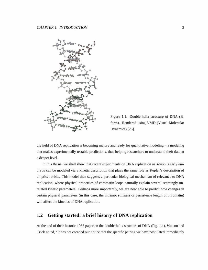
Figure 1.1: Double-helix structure of DNA (B-
form). Rendered using VMD (Visual Molecular
Dynamics) [26].
the field of DNA replication is becoming mature and ready for quantitative modeling – a modeling
that makes experimentally testable predictions, thus helping researchers to understand their data at
a deeper level.
In this thesis, we shall show that recent experiments on DNA replication inXenopusearly em-
bryos can be modeled via a kinetic description that plays the same role as Kepler’s description of
elliptical orbits. This model then suggests a particular biological mechanism of relevance to DNA
replication, where physical properties of chromatin loops naturally explain several seemingly un-
related kinetic parameters. Perhaps more importantly, we are now able to predict how changes in
certain physical parameters (in this case, the intrinsic stiffness or persistence length of chromatin)
will affect the kinetics of DNA replication.
1.2 Getting started: a brief history of DNA replication
At the end of their historic 1953 paper on the double-helix structure of DNA (Fig. 1.1), Watson and
Crick noted, “It has not escaped our notice that the specific pairing we have postulated immediately

CHAPTER 1. INTRODUCTION 4
suggests a possible copying mechanism for the genetic material.” [5]
A month later, in their second paper, Watson and Crick published their hypothesis for the repli-
cation of DNA: “semiconservative replication” [27]. Their basic idea was that, if the order of the
bases on one of the pairs of chains is given, then the exact order of the bases on the other one is de-
termined by a specific pairing of complementary bases [adenosine (A) with thymine (T), cystine (C)
with guanine (G)]. One can then think of the double-stranded DNA molecule as a pair of templates
for replication, each of which is complementary to the other. In other words, each single strand
acts as a template for the formation of a complementary DNA strand, so that each daughter DNA
molecule has the same sequence as the original one. Semiconservative replication was confirmed in
1958 by an elegant experiment by Meselson and Stahl [28].
How does a cell actually replicate DNA? If Watson and Crick were right, there should be an
enzyme that makes DNA copies from a DNA template. In 1956, Arthur Kornberg and colleagues
demonstrated the existence of such an enzyme: DNA polymerase I (pol I) ofE. coli bacteria, a
model prokaryote [29]. Indeed, the current paradigm of DNA replication traces back to Kornberg’s
pioneering discovery and his method of enzymology (see below, as well as Ref. [30]).
Schematically, to be able to replicate, a cell has to unfold and unwind its DNA. (As we shall
explain shortly, DNA is packed into a compact structure called chromatin.) It also has to separate the
two strands from each other. The cell has a complex machinery to perform these tasks [Fig. 1.2(a)].
When it is time to replicate, special initiator proteins attach to the DNA at regions called replication
origins. The initiator proteins pry the two strands apart, and a small gap is created at the replication
origin. Once the strands are separated, another group of proteins that carries out the DNA replication
attaches and goes to work.
This group of proteins includes helicase, which serves as an “unzipper” by breaking the bonds
between the two DNA strands. This unzipping takes place in both directions from the replication
origins, creating a replication bubble (or “eye”).4 The replication is therefore said to be bidirectional.
Once the two strands are separated, a small piece of RNA, called an RNA primer, is attached to the
DNA by an enzyme called DNA primase. These primers are the beginnings of all new DNA chains,
since DNA polymerases cannot start from scratch. It is a self-correcting enzyme and copies the
DNA template with remarkable fidelity.5
4The terms “replication bubble” or “eye” come from the appearance of DNA in early electron-microscopy work. (See
Fig. 1.5, below.)5As an example of this fidelity, consider a naive estimate for the base-pairing error rate that uses the free-energy

CHAPTER 1. INTRODUCTION 5
Helicase
Primase
Topoisomerase
Polymerase IIIdimer
Clamp
Ligase
Single-stranded DNABinding proteins
Polymerase I
5’ 3’
5’3’ 5’3’
Okazaki fragment
(a) (b)
Figure 1.2: Schematic model of replication fork. (a) Various enzymes and proteins that function
at or near a DNA replication fork (see text for details). The fork is moving upward. (b) Okazaki
fragment.
The DNA polymerase can read in only one direction (3′ to 5′). This gives rise to some trouble,
since the two strands of the DNA are antiparallel. On the upper strand, which runs from 3′ to
5′, nucleotide polymerisation can take place continuously without any problems. This strand is
called the “leading” strand. But how does the polymerase copy the other strand then when it runs
in the opposite direction, from 5′ to 3′? On this “lagging” strand the polymerase produces short
DNA fragments, called Okazaki fragments, by using a backstitching technique [Fig. 1.2(b)]. These
lagging strand fragments are primed by short RNA primers and are subsequently erased by pol I
and replaced by DNA with help of DNA ligase (Fig. 1.2). Meanwhile, as the fork progresses, DNA
becomes more and more twisted because of its double-helix structure, and it is topoisomerase that
“untwists” DNA.
As one can imagine, DNA replication is crucial to life and, thus, highly regulated, both tem-
difference between correct and incorrect base pairs. Since incorrect base pairs have an enthalpy (bonding + stacking)
several∼ kBT greater than the correct base pairs [31], one can use the Boltzmann distribution to estimate an error rate
of exp(∆E/kBT ) ∼ 10−2 − 10−4. In fact, the observed error rate is10−10 and is the result of an elaborate active
“proofreading” and correction scheme [32].

CHAPTER 1. INTRODUCTION 6
M
S
G1G2
M
S
(a) (b)
Early embryo(before MBT)
Figure 1.3: Eukaryotic cell cycle. (a) The two critical events of the cell cycle are S and M, which are
DNA replication (synthesis) and mitosis (nuclear and cell division), respectively. There are also gap
phases between the two. Normally, replication origins are replications are determined (“licensed")
in G1 before the cell enters S phase. G1, S, and G2 are collectively referred to as “interphase.” (b)
An embryonic cell cycle lacks the Gap phases.
porally and spatially. But, when and where does initiation actually occur? How many replications
origins are there along the genome?
The answers to many of these questions are well-understood for prokaryotes, which usually have
circular DNA and a single unique origin [30]. For example,E. coli has a specific site called oriC
(245 bp long) where a complex of DnaA proteins bind and starts replication. The replication bubble
then grows bidirectionally (at a rate≈ 1000 bp/sec) and terminates at another site called terC. The
whole 4.7 million basepairs (bp) are completely duplicated in less than 40 minutes. What about
eukaryotes? The answer is similar but much more complex. First, eukaryotic cells go through a
series of stages, called a cell cycle [Fig. 1.3(a)], and DNA is only replicated during one of those
stages called S phase (not surprisingly, “S” stands for synthesis) [Fig. 1.3(a)]. Second, eukaryotic
genomes are usually much longer than prokaryotic ones. The human genome, for example, consists
of 23 (pairs of) chromosomes with a total length of3× 109 bp. Here, “chromosomes” refers to the
threadlike “packages” of genes in the cell nucleus (Fig. 1.4). In contrast to prokaryotic systems, the
replication fork velocities are of order 10 bp/sec. Because the S phase can be as short as 20 minutes,
replication must take place simultaneously at many different sites along the DNA. Indeed, with fork

CHAPTER 1. INTRODUCTION 7feature
NATURE | VOL 421 | 23 JANUARY 2003 | www.nature.com/nature 449
may facilitate gene activation, by promoting specific structural interactions between distal sequences, or repression, by occludingbinding sites for transcriptional activators.
We suggest that the function of archaeal histones reflects theirancestral function, and therefore that chromatin evolved originallyas an important mechanism for regulating gene expression. Its use in
packaging DNA was an ancillary benefit that was recruited for themore complex nucleosome structure that subsequently evolved inthe ancestors of modern eukaryotes, which had expanded genomesizes. Although their compactness might seem to suggest inertness,chromatin structures are in fact a centre for a range of biochemicalactivities that are vital to the control of gene expression, as well asDNA replication and repair.
Packaging DNA into chromatinThe fundamental subunit of chromatin is the nucleosome, whichconsists of approximately 165 base pairs (bp) of DNA wrapped in twosuperhelical turns around an octamer of core histones (two each ofhistones H2A, H2B, H3 and H4). This results in a five- to tenfoldcompaction of DNA6. The DNA wound around the surface of the histone octamer (Fig. 1) is partially accessible to regulatory proteins,but could become more available if the nucleosome could be movedout of the way, or if the DNA partly unwound from the octamer. Thehistone ‘tails’ (the amino-terminal ends of the histone proteinchains) are also accessible, and enzymes can chemically modify thesetails to promote nucleosome movement and unwinding, with profound local effects on the chromatin complex.
Each nucleosome is connected to its neighbours by a short segment of linker DNA (~10–80 bp in length) and this polynucleo-some string is folded into a compact fibre with a diameter of ~30 nm,producing a net compaction of roughly 50-fold. The 30-nm fibre isstabilized by the binding of a fifth histone, H1, to each nucleosomeand to its adjacent linker. There is still considerable debate about thefiner points of nucleosome packing within the chromatin fibre, andeven less is known about the way in which these fibres are furtherpacked within the nucleus to form the highest-order structures.
Chromatin regulates gene expression Regulatory signals entering the nucleus encounter chromatin, notDNA, and the rate-limiting biochemical response that leads to activation of gene expression in most cases involves alterations inchromatin structure. How are such alterations achieved?
The most compact form of chromatin is inaccessible and therefore provides a poor template for biochemical reactions such astranscription, in which the DNA duplex must serve as a template forRNA polymerase. Nucleosomes associated with active genes wereshown to be more accessible to enzymes that attack DNA than thoseassociated with inactive genes7, which is consistent with the idea thatactivation of gene expression should involve selective disruption ofthe folded structure.
Clues as to how chromatin is unpacked came from the discovery thatcomponents of chromatin are subject to a wide range of modificationsthat are correlated with gene activity. Such modifications probablyoccur at every level of organization, but most attention has focused onthe nucleosome itself. There are three general ways in which chromatinstructure can be altered. First, nucleosome remodelling can be inducedby complexes designed specifically for the task8; this typically requiresthat energy be expended by hydrolysis of ATP. Second, covalent modifi-cation of histones can occur within the nucleosome9. Third, histonevariants may replace one or more of the core histones10–12.
Some modifications affect nucleosome structure or labilitydirectly, whereas others introduce chemical groups that are recog-nized by additional regulatory or structural proteins. Still others maybe involved in disruption of higher-order structure. In some cases,the packaging of particular genes in chromatin is required for theirexpression13. Thus, chromatin can be involved in both activation andrepression of gene expression.
Chromatin remodellingTranscription factors regulate expression by binding to specific DNAcontrol sequences in the neighbourhood of a gene. Although someDNA sequences are accessible either as an outward-facing segmenton the nucleosome surface, or in linkers between nucleosomes, most
30-nm chromatinfibre of packednucleosomes
Section ofchromosome in anextended form
Condensed sectionof chromosome
Entire mitoticchromosome
Centromere
Short region ofDNA double helix
2 nm
11 nm
700 nm
1,400 nm
30 nm
300 nm
"Beads on a string"form of chromatin
a
b
Figure 1 Packaging DNA. a, The organization of DNA within the chromatin structure.The lowest level of organization is the nucleosome, in which two superhelical turns ofDNA (a total of 165 base pairs) are wound around the outside of a histone octamer.Nucleosomes are connected to one another by short stretches of linker DNA. At thenext level of organization the string of nucleosomes is folded into a fibre about 30 nmin diameter, and these fibres are then further folded into higher-order structures. Atlevels of structure beyond the nucleosome the details of folding are still uncertain.(Redrawn from ref. 41, with permission). b, The structure of the nucleosome coreparticle was uncovered by X-ray diffraction, to a resolution of 2.8Å (ref. 42). It showsthe DNA double helix wound around the central histone octamer. Hydrogen bondsand electrostatic interactions with the histones hold the DNA in place.
© 2003 Nature Publishing Group
Figure 1.4: Higher-order struc-
ture of chromatin. Courtesy
of Gary Felsenfeld and Mark
Groudine. Reprinted by per-
mission from Nature [vol.421,
pp. 448-453] copyright (2003)
Macmillan Publishers Ltd.
velocities 100 times slower and with 1000 times the DNA to replicate, the eukaryotic genome can
have as many as105 origins of replication (Fig. 1.5), often with different growth rates.
Because of these complexities, there are still many basic questions waiting to be answered. For
example, what regulates the spatio-temporal distributions of replication bubbles during the course
of S phase? What ensures that DNA is replicated once and only once during S phase? Are there
specific sequences of DNA that are responsible for initiation in eukaryotes? Does a higher-order
structure of chromatin and/or other structures inside the cell nucleus play a role in DNA replication?
As a more specific example, we briefly summarize the process of DNA replication in one of
the best-studied eukaryotic systems, the famous South African clawed toadXenopus laevis. (For
detailed reviews, see Refs. [34, 35].)

CHAPTER 1. INTRODUCTION 8
Figure 1.5: Electron micrograph showing multiple replication bubbles ofDrosophila melanogaster
DNA. From Fig. 2 in Ref. [33] by Kriegstein and Hogness, with permission. Copyrightc© Proceed-
ings of the National Academy of Sciences USA.
The fertilizedXenopusegg undergoes 12 synchronous rounds of cell division in about 8 hours.
During this period, the large egg (≈ 1 mm) subdivides into 4096 (= 212) smaller cells without
growing in size. After the first 12 cycles of cleavage, the cell-division rate slows down abruptly, and
transcription (protein synthesis) of the embryo’s genome begins. This change is known as the mid-
blastula transition (MBT). Since its large eggs are easy to manipulate and see and since its cell cycle
is rapid and simple,6 the early-embryoXenopusis a good model for studying cell-cycle regulation.
An interesting (and important) fact aboutXenopusearly embryos is that, unlikeE. colior another
simple eukaryote, budding yeast, there is no specific sequence requirement for initiating DNA repli-
cation [36]. Moreover, these early embryos lack an efficient S/M checkpoint that makes cells delay
entry into mitosis in the presence of unreplicated DNA [37]. Nevertheless, theXenopusdiploid
genome ( > 6 billion basepairs!) is completely replicated within the 10-20 minutes of S phase. Ap-
parently, there is a strict control mechanism, independent of sequence, that regulates the density of
origins and time of activation to prevent the “random-completion problem,” where any large fluctu-
ations in the spacing between origins would lead to (fatal) fluctuations in the duration of S phase.
One of the goals of this thesis is to study the spatio-temporal program of DNA replication in this
6Each cycle consists of only two stages: Mitosis (cell-division) and S phase; see Fig. 1.3(b). Also, note that during S
phase in early embryos, no proteins are synthesized [32].
CHAPTER 1. INTRODUCTION 9
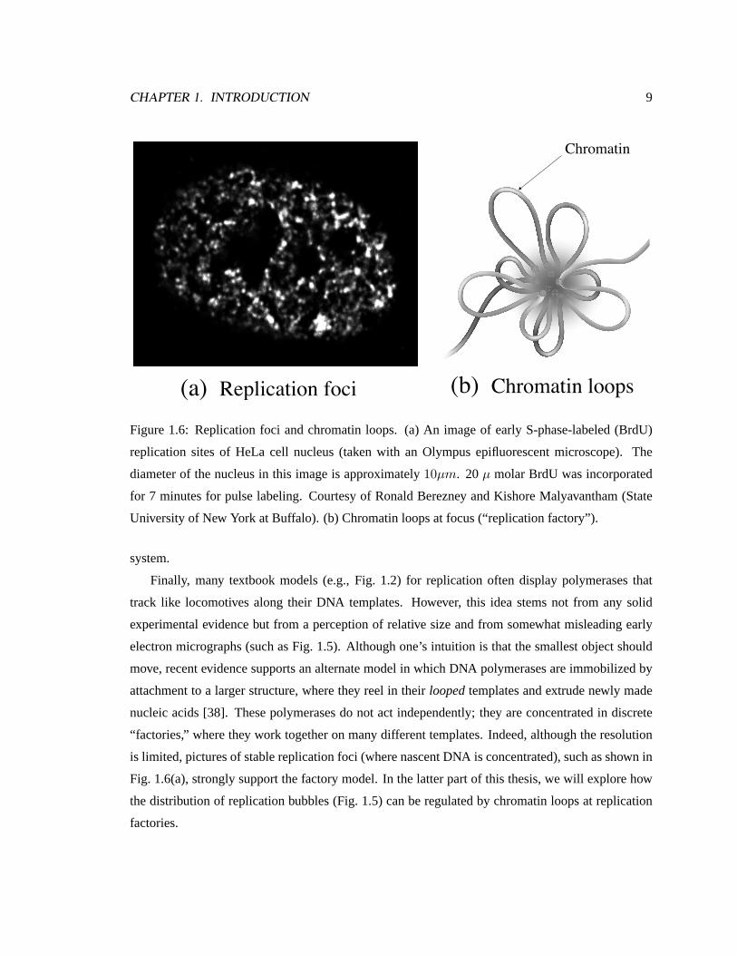
Chromatin
(a) Replication foci (b) Chromatin loops
Figure 1.6: Replication foci and chromatin loops. (a) An image of early S-phase-labeled (BrdU)
replication sites of HeLa cell nucleus (taken with an Olympus epifluorescent microscope). The
diameter of the nucleus in this image is approximately10µm. 20µ molar BrdU was incorporated
for 7 minutes for pulse labeling. Courtesy of Ronald Berezney and Kishore Malyavantham (State
University of New York at Buffalo). (b) Chromatin loops at focus (“replication factory”).
system.
Finally, many textbook models (e.g., Fig. 1.2) for replication often display polymerases that
track like locomotives along their DNA templates. However, this idea stems not from any solid
experimental evidence but from a perception of relative size and from somewhat misleading early
electron micrographs (such as Fig. 1.5). Although one’s intuition is that the smallest object should
move, recent evidence supports an alternate model in which DNA polymerases are immobilized by
attachment to a larger structure, where they reel in theirloopedtemplates and extrude newly made
nucleic acids [38]. These polymerases do not act independently; they are concentrated in discrete
“factories,” where they work together on many different templates. Indeed, although the resolution
is limited, pictures of stable replication foci (where nascent DNA is concentrated), such as shown in
Fig. 1.6(a), strongly support the factory model. In the latter part of this thesis, we will explore how
the distribution of replication bubbles (Fig. 1.5) can be regulated by chromatin loops at replication
factories.

CHAPTER 1. INTRODUCTION 10
1.3 About this thesis
The main goal of this thesis is to develop and present various tools in theoretical physics that can
be used to identity the spatio-temporal program of DNA replication from data. We then apply our
methods to recent experiments on a model system,Xenopusegg extracts, which support all the
nuclear events of the early embryonic cell-division cycle.
Our starting point is the electron micrograph of multiple eyes in Fig. 1.5, which we interpret
as a “snapshot” of a one-dimensional system undergoing nucleation-and-growth processes with an
unknown nucleation rateI(t). This mapping of the description of DNA replication onto the de-
scription of (one-dimensional) crystal-growth kinetics gives us access to a well-developed set of
theories.7 Thus, in Ch. 2, we introduce the classic Kolmogorov-Johnson-Mehl-Avrami model of
nucleation and growth [39–43] and extend it to the case of an arbitrary nucleation functionI(t).
In Ch. 3, we study the reverse, ı.e., we discuss how to extractI(t) from a set of many snapshots
analogous to Fig. 1.5. In Ch. 4, we apply the kinetic model to data recently obtained by Herricket
al. [44]. We then discuss the extractedI(t) as a temporal program of replication inXenopusearly
embryos.
In the next two chapters, we shift our focus to understanding the biological mechanisms that
underlie the replication program. This leads us to consider the replication-factory model. (Fig. 1.6)
Since one of the possible implications of the factory model is that chromatin fibers should attach to
immobilized factories via looping, the loop sizes should correspond to the origin spacings. As we
shall show later, the loop-formation probability depends on the intrinsic stiffness (or “persistence
length”) of polymers, and there is a specific length where loops can form most efficiently. In Ch. 5,
we incorporate these results into the kinetic model to explain the spatial distribution of replication
bubbles in the experimental data. Two crucial assumptions here are that, first, the loop-formation
time is much shorter than the typical time-scale of DNA replication such as the duration of S phase.
Second, we assume that the sizes of loops formed represent those with largest statistical weight, as
calculated via an equilibrium distribution of loop-sizes. In Ch. 6, we tackle a simplified version of
the problem, namely, loop-formation dynamics of a single chain with two “sticky” ends. We obtain a
simple analytical expression to estimate the closing timeτc, and, indeed, a typicalτc for chromatin is
7We emphasize that one should not interpret Fig. 1.5 as the actual geometry of DNA in a cell nucleus during replication.
Even so, the one-dimensional topology of alternating replicated and non-replicated domains is still correct, and our model
will be based on this topology.

CHAPTER 1. INTRODUCTION 11
several orders of magnitude smaller than the duration of S phase. In addition, in certain (biologically
relevant) limits, the loop-formation rate of polymers is set by the equilibrium distributions of loop
sizes, thus justifying the results in Ch. 5.
The results in Ch. 4 and 5 can be considered to provide a mechanism that ensures complete,
faithful, and timely reproduction of the genome without any sequence dependence of replication
origins inXenopusearly embryos.
Parts of this thesis are based on previously published our work: Ch. 4 on Ref. [59], Ch. 5 on
Ref. [71], and Ch. 6 on Ref. [155].

Chapter 2
The Generalized
Kolmogorov-Johnson-Mehl-Avrami
Model
2.1 Introduction
Consider a tray of water that at timet = 0 is put into a freezer. A short while later, the water is all
frozen. One may thus ask, “What fractionf(t) of water is frozen at timet ≥ 0?” In the 1930s,
several scientists independently derived a stochastic model that could predict the form off(t),
which experimentally is a sigmoidal curve. The “Kolmogorov-Johnson-Mehl-Avrami” (KJMA)
model [39–43] has since been widely used by metallurgists and other materials scientists to analyze
phase transition kinetics [45]. In addition, the model has been applied to a wide range of other
problems, from crystallization kinetics of lipids [46], polymers [47], the analysis of depositions in
surface science [48], to ecological systems [49], and even to cosmology [50]. For further examples,
applications, and the history of the theory, see the reviews by Evans [51], Fanfoni and Tomellini [48],
and Ramoset al. [52].
In the KJMA model, freezing kinetics result from three simultaneous processes: 1) nucleation of
solid domains (“islands”); 2) growth of existing islands; and 3) coalescence, which occurs when two
expanding islands merge. In the simplest form of KJMA, islands nucleate anywhere in the liquid
areas (“holes”), with equal probability for all spatial locations (“homogeneous nucleation”). Once
12

CHAPTER 2. GENERALIZED KJMA MODEL 13
an island has been nucleated, it grows out as a sphere at constant velocityv. (The assumption of
constantv is usually a good one as long as temperature is held constant, but real shapes are far from
spherical. In water, for example, the islands are snowflakes; in general, the shape is a mixture of den-
dritic and faceted forms. The effect of island shape – not relevant to the one-dimensional version of
KJMA studied here – is discussed extensively in [45].) When two islands impinge, growth ceases at
the point of contact, while continuing elsewhere. KJMA used elementary methods, reviewed below,
to calculate quantities such as the solid fractionf(t). Later researchers have revisited and refined
KJMA’s methods to take into account various effects, such as finite system size and inhomogeneities
in growth and nucleation rates [53–55].
Although most of the applications of the KJMA model have been to the study of phase trans-
formations in three-dimensional systems, similar ideas have been applied to a wide range of one-
dimensional problems, such as Rényi’s car-parking problem [56] and the coarsening of long parallel
droplets [57]. In this thesis, we shall apply the KJMA model to DNA replication in higher organ-
isms. We start by observing that the duplication of eukaryotic genomes shares a number of common
features [58] that can be mapped onto the basic assumptions of the KJMA model [59]:
1. DNA replication starts at a large number of sites known as “origins of replication.” The DNA
domain replicated from each origin is referred to, informally, as an “eye” or a “replication
bubble” because of its appearance in electron microscopy. (Fig. 1.5.)
2. The position of each potential origin that is “competent” to initiate DNA replication is de-
termined before the beginning of the synthesis part of the cell cycle (“S phase”), when sev-
eral proteins including the origin recognition complex (ORC) bind to DNA, forming a pre-
replication complex (pre-RC).
3. During S phase, a particular potential origin may or may not be activated. Each origin is
activated not more than once during the cell-division cycle.
4. DNA synthesis propagates at replication forks bidirectionally, with propagation speed or fork
velocityv, from each activated origin. Experimentally,v is approximately constant throughout
S phase.
5. DNA synthesis stops when two newly replicated regions of DNA meet.
From Fig. 2.1, it is apparent that processes 3–5 have a formal analogy with nucleation and growth
in one dimension (see also Fig. 1.5). We identify (1) nucleation of islands as activation (initiation)

CHAPTER 2. GENERALIZED KJMA MODEL 14
nucleation
islandhole
initiation
eyehole
(a) (b) KJMADNA replication
t1
t2
t3
t4
t5
t6
island-to-island
Figure 2.1: Mapping DNA replication onto the one-dimensional KJMA model.
of replication origins; (2) growth of the eyes as growth of the islands; and (3) coalescence of two
expanding eyes as the merging of growing islands. Of course, while DNA is topologically one
dimensional, it is embedded in a three-dimensional space.
In an ideal world, one could monitor the replication process continuously and compile domain
statistics in real time. In the real world, the three billion DNA basepairs (bp) of a typical higher
eukaryote, which replicate in as many as∼105 sites simultaneously, are packed in a cell nucleus
of radius∼1 µm, making a direct, real-time monitoring impossible [32]. In Ch. 4, we analyze an
experiment that used two-color fluorescent labeling of DNA bases to study replication kinetics indi-
rectly (Fig. 2.2).1 Schematically, one begins (in a test tube) by labeling the bases used in replicating
the DNA with, say, a red dye. At some time during the replication process (e.g.,t1 in Fig. 2.1),
one floods the test tube with green-labeled bases and allows the replication cycle to go to comple-
tion. One then stretches the DNA onto a glass slide (“molecular combing” [23]), a process that
unfortunately also breaks the DNA strands into finite segments. Under a microscope, regions that
replicated before adding the dye are red, while those labeled afterwards are predominantly green.
Typical two-color epifluorescence images of the combed DNA are shown in Fig. 2.3. The red-and-
green regions correspond to eyes and holes in Fig. 2.1, forming a kind of snapshot of the replication
state of the DNA fragment at the time the second dye was added. Each time point in Fig. 2.1 would
1The experimental details are described elsewhere [44], but the approach is similar to DNA fiber autoradiography
developed by Huberman and Riggs, a method that has been in use for the last 30 years [60, 61].

CHAPTER 2. GENERALIZED KJMA MODEL 15
DNAsolution
coverslipmeniscus
(a) (b) (c) (d)biotin-dUTP dig-dUTP
“eye”
Xenopus egg extracts+ sperm chromatin
Figure 2.2: Schematic description of the double-labeling experiment. (a) Before replication starts,
one adds “red dye” (biotin-dUTP) into the solution ofXenopusegg extracts and sperm chromatin.
(b) “Eyes” then grow while more replication origins fire. (c) At chosen time points, one adds “green
dye” (dig-dUTP) and waits until the DNA is completely replicated. (d) One then stretches the
replicated DNA molecules in solution onto a glass surface (“molecular combing”). For more details,
see text and Ref. [44].
thus correspond to a separate experiment.
The purpose of the present two chapters, then, is as follows: Here, in Ch. 2, we discuss the
KJMA model and how to generalize it for biological application. In particular, we consider the
problem of arbitrarily varying origin initiation rate (equivalent to arbitrarily varying nucleation rate
in freezing processes). Then, in Ch. 3, we discuss a number of subtle but generic issues that arise
in the application of the KJMA model to DNA replication. The most important of these is that the
method of analysis runs backward from the usual one. Normally, one starts from a known nucle-
ation rate (determined by temperature, mostly) and tries to deduce properties of the crystallization
kinetics. In the biological experiments, the reverse is required: from measurements of statistics
associated with replication, one wants to deduce the initiation rateI(t). This problem, along with
others relating to inevitable experimental limitations, merits separate consideration.
In the mid-1980s, Sekimoto showed that the analysis of the KJMA model could be pushed
much further if growth occurs in only one spatial dimension [62–64]. Sekimoto used methods from
non-equilibrium statistical physics to describe the detailed statistics of domain sizes and spacings,
as defined in Fig. 2.1. In particular, he studied the time evolution of domain statistics by solving

CHAPTER 2. GENERALIZED KJMA MODEL 16
Figure 2.3: A fluorescence micrograph (bar= 20 µm). Early replicating sequences labeled with
biotin-dUTP are visualized using red fluorescing antibodies (Texas Red). Later replicating se-
quences are in addition labeled with dig-dUTP and visualized using green (FITC) fluorescing anti-
bodies. Courtesy of Aaron Bensimon and John Herrick.
Fokker-Planck-type equations for island and hole distributions, assuming that the nucleation rate
I(t) is constant. His approach has since been revisited by others (e.g., [65]).
Below, we review Sekimoto’s approach and extend it to the case of an arbitrary nucleation rate
I(t). As mentioned above, this case is relevant to the kinetics of DNA replication in eukaryotes. We
also present an algorithm to simulate 1D nucleation-and-growth processes that is much faster than
more-standard lattice methods [66].

CHAPTER 2. GENERALIZED KJMA MODEL 17
1
0
f(t)t
∆x∆t
0time
2vt
(a) X
€
~ 1I0v
1(b)
0 t
Figure 2.4: Kolmogorov’s method for constant nucleation rateI(t) = I0. (a) Spacetime diagram.
In the small square box, the probability of nucleation isI0 ·∆x ·∆t, whereI0 is the nucleation rate.
In order for the pointX to remain uncovered by islands, there should be no nucleation in the shaded
triangle in spacetime. (b) Kinetic curve for constant nucleation rateI0: f(t) = 1− exp(−I0vt2).
2.2 Theory
2.2.1 Island fractionf(t)
We begin with the calculation off(t), the fraction of islands at timet in a one-dimensional system.
We write asf(t) = 1 − S(t), whereS(t) is the fraction of the system uncovered by islands (ı.e.,
the hole fraction). In other words,S(t) is the probability for an arbitrary pointX at timet to remain
uncovered. If we view the evolution via a two-dimensional spacetime diagram [Fig. 2.4(a)], we can
calculateS by noting that
S(t) = lim∆x,∆t→0
∏x,t∈4
(1− I0∆x∆t)
= exp(−
∫∫x,t∈4
I0dxdt
)(2.1)
= exp(−I0vt2).
Therefore,
f(t) = 1− e−I0vt2 , (2.2)
which has a sigmoidal shape, as mentioned above [see Fig. 2.4(b)].
We note that Kolmogorov’s method can be straightforwardly applied to any spatial dimensionD
for arbitrary time- and space-dependent nucleation ratesI(~x, t). Similar “time-cone” methods can
yield f(t) in the presence of complications such as finite system sizes [53–55]. Unfortunately, this
CHAPTER 2. GENERALIZED KJMA MODEL 18
€
ρh x, t( )
€
ρh x, t + dt( )
Domain size x
Dist
ribut
ion
€
2v ⋅ dtnucleation
x
nucleation
yx
(a) (b)
(c)
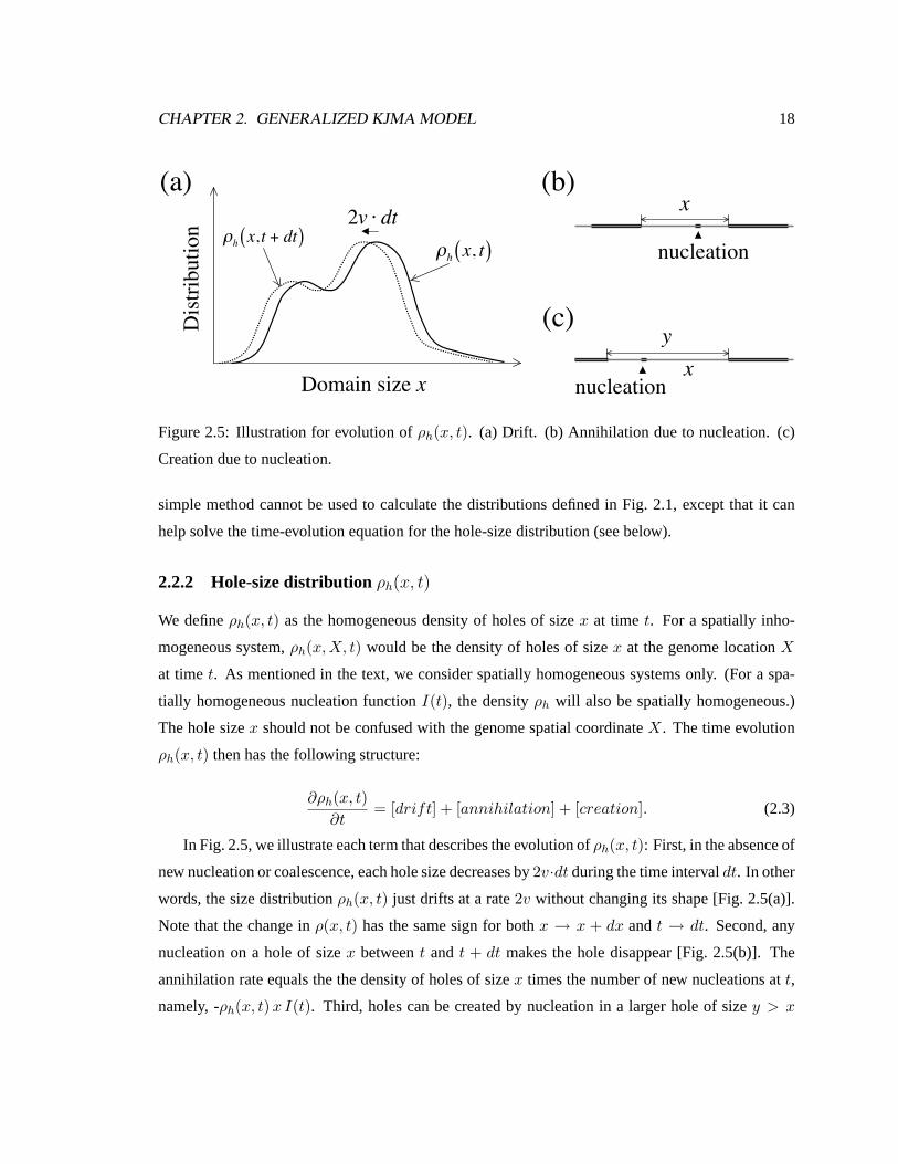
Figure 2.5: Illustration for evolution ofρh(x, t). (a) Drift. (b) Annihilation due to nucleation. (c)
Creation due to nucleation.
simple method cannot be used to calculate the distributions defined in Fig. 2.1, except that it can
help solve the time-evolution equation for the hole-size distribution (see below).
2.2.2 Hole-size distributionρh(x, t)
We defineρh(x, t) as the homogeneous density of holes of sizex at timet. For a spatially inho-
mogeneous system,ρh(x, X, t) would be the density of holes of sizex at the genome locationX
at timet. As mentioned in the text, we consider spatially homogeneous systems only. (For a spa-
tially homogeneous nucleation functionI(t), the densityρh will also be spatially homogeneous.)
The hole sizex should not be confused with the genome spatial coordinateX. The time evolution
ρh(x, t) then has the following structure:
∂ρh(x, t)∂t
= [drift] + [annihilation] + [creation]. (2.3)
In Fig. 2.5, we illustrate each term that describes the evolution ofρh(x, t): First, in the absence of
new nucleation or coalescence, each hole size decreases by2v·dt during the time intervaldt. In other
words, the size distributionρh(x, t) just drifts at a rate2v without changing its shape [Fig. 2.5(a)].
Note that the change inρ(x, t) has the same sign for bothx → x + dx andt → dt. Second, any
nucleation on a hole of sizex betweent and t + dt makes the hole disappear [Fig. 2.5(b)]. The
annihilation rate equals the the density of holes of sizex times the number of new nucleations att,
namely, -ρh(x, t) x I(t). Third, holes can be created by nucleation in a larger hole of sizey > x

CHAPTER 2. GENERALIZED KJMA MODEL 19
x
t∆x
∆t
Island-to-island (i2i) Island (i)
Hole (h)
A D
B C
Figure 2.6: Spacetime diagram. The hole-size distributionρh(x, t) is proportional to the probability
p0(x, t) for no nucleation event occurs in the shaded parallelogramABCD (see text).
[Fig. 2.5(c)].
Based on the arguments above, we obtain
∂ρh(x, t)∂t
= 2v∂ρh(x, t)
∂x− I(t) x ρh(x, t) + 2I(t)
∫ ∞
xρh(y, t)dy, (2.4)
where the factor 2 in the last (creation) term comes from the left- and right-symmetry of the nucle-
ation process.
Eq. 2.4 was solved by Sekimoto forI(t)=const., while Ben-Naimet al. derived a formal solution
for arbitraryI(t) [67]. Below, we show that the solution of Ben-Naimet al. can also be obtained
directly by applying Kolmogorov’s argument.
In Fig. 2.6, we see a hole of sizex flanked by two islands. In order for such holes to exist at
time t, there should be no nucleation within the parallelogramABCD in the spacetime diagram.
Similar to the calculation of the hole fractionS(t), we obtain the “no nucleation” probability in the
parallelogram as
p0(t) = lim∆x,∆t→0
∏x,t∈ABCD
[1− I(t)∆x∆t]
= S(t)e−g(t)·x. (2.5)
whereg(t) =∫ t0 I(t′)dt′. The domain densityn(t) and the hole fractionS(t) are related by defini-

CHAPTER 2. GENERALIZED KJMA MODEL 20
tion as follows:
n(t) =∫ ∞
0ρh(x, t)dx (2.6)
S(t) =∫ ∞
0x ρh(x, t)dx. (2.7)
Since the hole-size distributionρh(x, t) is proportional top0(x, t), we can writeρh(x, t) = c(t) ·p0(x, t). By integrating this equation and using Eq. 2.6, we obtainc(t) = n(t) · g(t)/S(t). Putting
this back into Eq. 2.4, we obtain an equation forn(t):
1n(t)
∂n(t)∂t
= −2v · g(t) +I(t)g(t)
. (2.8)
This is a first-order linear equation and can be solved exactly. Using the boundary conditionn(0) =
1, we solve Eqs. 2.8 and 2.4 to find
n(t) = g(t) · e−2vR t0 g(t′)dt′ ; (2.9)
ρh(x, t) = g(t)2 · e−g(t)x−2vR t0 g(t′)dt′ . (2.10)
These are just exponential functions ofx, with decay constants that monotonically decrease as a
function of time.
2.2.3 Island distribution ρi(x, t)
In analogy to Eq. 2.4 and following [63], a time-evolution equation can be obtained for the island-
size distributionρi(x, t). In this case, the drift term is the same as in Eq. 2.4, except that the sign
changes because islands always grow. On the other hand, new nucleations contribute toρi(x, t)
only with sizeless (x = 0) islands with a rate−δ(x) ·∫∞0 I(t) x ρh(x, t) dx = −I(t) S(t) δ(x) (see
Eq. 2.6). Finally, coalescence of two islands can both annihilate and create islands of sizex: for
annihilation, either of the islands should have a sizex; for creation, the sum of the sizes of the two
islands should bex. The resulting equation can be written as
∂ρi(x, t)∂t
= −2v∂ρi(x, t)
∂x+ I(t) S(t) δ(x) + a(t)
[ ∫ x
0ρi(x− y, t)ρi(y, t)dy − 2n(t)ρi(x, t)
],
(2.11)
wherea(t) is a prefactor that should be determined. We recall that, in one-dimension, both holes and
islands have the same domain densityn(t) =∫∞0 ρ(x, t)dx. This means thata(t) can be determined

CHAPTER 2. GENERALIZED KJMA MODEL 21
by applying∫∞0 dx to Eqs. 2.4 and 2.12 and comparing the two, as follows:
∂n(t)∂t
= −2vρh(0, t)− I(t) S(t) + 0
∂n(t)∂t
= 0− I(t) S(t) + a(t) · [n(t)2 − 2 n(t)2].
Thus,a(t) = 2v ρ(0, t)/n(t)2 and we obtain
∂ρi(x, t)∂t
= −2v∂ρi(x, t)
∂x+ I(t) S(t) δ(x)
+2vρh(0, t)n(t)2
[ ∫ x
0ρi(x− y, t)ρi(y, t)dy − 2n(t)ρi(x, t)
]. (2.12)
Unfortunately, we cannot solve Eq. 2.12 using the simple arguments that worked forρh(x, t).
The main difference is that a hole is created bynucleationonly, while an island of nonzero size
is created by growth and/or thecoalescenceof two or more islands. Thus,ρi(x, t) is given by an
infinite sum of probabilities for an island to contain one seed, two seeds, three seeds, and so on.
Nevertheless, we can still obtain the asymptotic behavior ofρi(x, t) for arbitraryI(t) by Laplace
transforming the above evolution equation, as in [63].
Applying∫∞0 dxe−sx to Eq. 2.12, we find
∂ρi(s, t)∂t
= −2v [s + 2g(t)] ρi(s, t) + 2v e2vR t0 g(t′)dt′ · ρi(s, t)2 + I(t) S(t), (2.13)
whereρi(s, t) ≡∫∞0 e−sxρi(x, t)dx, with initial conditionsρi(s, 0) = 0. We can further simplify
Eq. 2.13 by definingGi(s, t) = exp[2v
∫ t0 g(t′)dt′
]· ρi(s, t), which then obeys
∂Gi(s, t)∂t
= −2v [s + g(t)] Gi(s, t) + 2v Gi(s, t)2 + I(t). (2.14)
If we write Gi(s, t) as
Gi(s, t) = s + g(t) + X(s, t), (2.15)
we find thatX(s, t) obeys the (nonlinear) Bernoulli equation [68]:
∂X(s, t)∂t
= [s + g(t)] X(s, t) + X(s, t)2. (2.16)
Solving Eq. 2.16 and substituting back into Eq. 2.15, we find the Laplace transformρi(s, t):
ρi(s, t) = e−2vR t0 g(t′)dt′ Gi(s, t) (2.17)
= e−2vR t0 g(t′)dt′
{s + g(t)−
s · exp[2v(st +∫ t0 g(t′)dt′)]
1 + 2v · s∫ t0 exp[2v(st′ +
∫ t′
0 g(t′′)dt′′)]dt′
}.

CHAPTER 2. GENERALIZED KJMA MODEL 22
We cannot perform the inverse Laplace transform of the above equation, even for the simple
case ofI(t)=const. [ı.e.,g(t) ∼ t] [63, 65]. However, from the form of denominator in Eq. 2.17,
we observe thatρi(s, t) has a single simple pole along the negative real-axis at|s = s∗(t)| � 1
for t � 1, regardless of the form thatg(t) may have. Since the inverse Laplace transform can be
written formally as the Bromwich integral in the complex plane (ı.e., as the sum of residues of the
integrand [69]), a standard strategy for obtaining an asymptotic approximation toρi(x, t) for x � 1
is to expandρi(s, t) arounds∗(t) (|s∗(t)| � 1) to lowest order. Following Sekimoto’s approach, we
defineK(s, t) to be the denominator in Eq. 2.17, which becomes
ρi(s, t) = e−R t0 g(t′)dt′
[s + g(t)− 1
2v
∂K(s, t)∂t
1K(s, t)
],
Arounds = s∗(t), Eq. 2.17 can be approximated as
ρi(s, t) ' e−R t0 g(t′)dt′
−2v
∂K(s∗(t), t)∂t
1∂K(s∗(t),t)
∂s [s− s∗(t)]
= +e−
R t0 g(t′)dt′
2v
ds∗(t)dt
1s− s∗(t)
. (2.18)
From Eq. 2.18, we arrive at the following asymptotic expression forρi(x, t):
ρi(x, t) ' e−R t0 g(t′)dt′
2v
ds∗(t)dt
e−|s∗(t)|·x, (2.19)
for x, t � 1. Now, both the prefactor and the exponent [the poles∗(t)] can be obtained very easily
by simple numerical methods. On the other hand, an approximate expression fors∗(t) itself can
be found by first expandingK(s, t) in powers ofst and then solving iteratively using Newton’s
method [70]. (See Fig. 2.7) The result is
s∗(t) ' − 1J0
(1 +
J1
J20
+4J2
1 − J0J2
2J40
), (2.20)
where
Jn ≡∫ t
0e
R τ0 g(t′)dt′τndτ.
As we shall show below, Eq. 2.19 describes the behavior ofρi(x, t) accurately forx & 2vt.
2.2.4 Island-to-island distribution ρi2i(x, t)
While most studies of 1D nucleation-growth have focused onρh(x, t) andρi(x, t) exclusively, the
distribution of the distances between the centers of two adjacent islands [the island-to-island dis-
tribution ρi2i(x, t)] has important applications. For instance, whether homogeneous nucleation is a

CHAPTER 2. GENERALIZED KJMA MODEL 23
s*(t)
t
Numerical solution
Eq. 2.20
Figure 2.7: Plot ofs∗(t). The solid line is a direct numerical solution ofK(s, t) = 0 and the dashed
line is Eq. 2.20.
valid assumption cannot be knowna priori. Indeed, in the recent DNA replication experiment that
motivated this work, the “nucleation” sites for DNA replication along the genome were found to be
not distributed randomly, a result that has important biological implications for cell-cycle regula-
tion [71].
In the 1D KJMA model, Sekimoto has shown that a constant nucleation functionI0 cannot
produce correlations between domain sizes [63, 64]. We speculate that the same holds true for any
local nucleation functionI(x, t), a conclusion that is also supported by computer simulation2 [71].
Assuming a local nucleation function, we can write the formal expression forρi2i(x, t) directly in
terms ofρi(x, t) andρh(x, t):
ρi2i(x, t) = c
∫{i1,h,i2}∈S
ρi(i1, t)ρh(h, t)ρi(i2, t)dS, (2.21)
whereS designates the constraint plane shown in Fig. 5.3 [S : (i1 + i2)/2+h=x]. The normal-
ization coefficientc can be obtained easily from the relation,∫∞0 ρi2i(x, t)dx =
∫∞0 ρi(x, t)dx =∫∞
0 ρh(x, t)dx = n(t). From Eq. 2.21 and Fig. 5.3, it is easy to see that∫∞0 ρi2i(x, t)dx = c[n(t)]3,
and, therefore,c = [n(t)]−2.
2Even for a 1D nucleation-and-growth system, spatial correlations can exist. For a theoretical study of deviations from
the KJMA, see, for example, [72]. Blowet al. [24] and Junet al. [71] present experimental evidence for size correlations
of domain statistics in biological systems.

CHAPTER 2. GENERALIZED KJMA MODEL 24
i1
i2
h
x
2x
2x
Si1 h i2
x
Figure 2.8: Constraint planeS : (i1 + i2)/2 + h = x.
Since the full solution forρi(x, t) is not known, we cannot integrate Eq. 2.21. However, we can
still obtain an asymptotic expression forρi2i(x, t) using Eqs. 2.9 and 2.19. Forx � 1, taking into
account the constraintS, we find
ρi2i(x, t) ∼∫{i1,h,i2}∈S
e−|s∗(t)|·i1−g(t)·h−|s∗(t)|·i2dS (2.22a)
∼ e−g(t)x + e−2|s∗(t)|x[− 1 + g(t)x− 2|s∗(t)|x
]. (2.22b)
As we shall show later, Eq. 2.22b is an excellent approximation for allx andt. Note that the first
term on the right-hand side has the same asymptotic behavior as the hole-size distributionρh(x, t),
while the exponential factor in the second term comes from the product of island-size distributions
∼ e−|s∗(t)|·i1 and∼ e−|s
∗(t)|·i2 . The asymptotic behavior ofρi2i(x, t) is dominated byρh(x, t) for
f < 0.5 and byρi(x, t) for f > 0.5 (see below). But, at all times, we emphasize thatρi2i(x, t)
is asymptotically exponential for largex. From the mathematical point of view, bothρi(x, t) and
ρh(x, t) have exponential tails at largex, and the integral of the product of exponential functions
again produces an exponential.

CHAPTER 2. GENERALIZED KJMA MODEL 25
i0 h0 i1
h1i2
h2
h2’ = h0 +h1 +h2i22h1’ = h0 +h1
i11h0’ = h0i00
{h’}{i}
i0 i1 i2
h0’
h2h0 h1
h1’h2’
{i}
{h’}
h2’i22h1’i11h0’i00
{h’}{i}
h2’ = old h1’ i2 = 02
h3’ = old h2’ i3 = old i23
h1’ = x i11 h0’ i00 {h’}{i}
i0 h0 i1
h1i2
h2
i0 i1 i2
h0’ h1’ h2’
x
Before nucleation
After nucleation
i0h0
i1h1 << 1i2
h2 h2’ = h0 + 0 + h2i22h1’ = h0 + 0i11h0’ = h0i00 {h’}{i}
h1’ = old h2’old (i1+ i2)1 h0’ = h0i00 {h’}{i}
i0 h0
new i1
new h1
Before coalescence
After coalescence
(a)
(b)
(c)
x
Random number between 0 and h2’
Figure 2.9: Schematic description
of the double-list algorithm. (a) Ba-
sic set-up for lists{i} and {h′}.Note that{h′} records cumulative
lengths. (b) Nucleation. (c) Coales-
cence due to growth.

CHAPTER 2. GENERALIZED KJMA MODEL 26
2.3 Numerical simulation
Often, one has to deal with systems for which analytical results are difficult, if not impossible,
to obtain. For example, the finite size of the system may affect its kinetics significantly, or the
variation of growth velocity at different regions and/or different times could be important. In such
cases, computer simulation is the most direct and practical approach.
For one-dimensional KJMA processes, the most straightforward simulation method is to use an
Ising-model-like lattice, where each lattice site is assigned either 1 or 0 (or -1, for the Ising model)
representing island and hole, respectively. The natural lattice size is∆x = v ·∆t, with v the growth
velocity. At each timestep∆t of the simulation, every lattice site is examined. If 0, the site can be
nucleated by the standard Monte Carlo procedure, ı.e., a random number is generated and compared
with the nucleation probabilityI(t) · ∆x · ∆t. If the random number is larger than the nucleation
probability, the lattice site switches from 0 to 1. Once nucleation is done, the islands grow by∆x,
namely, by one lattice size at each end.
Although straightforward to implement, the lattice model is slow and uses more memory than
necessary, as one stores information not only for the moving domain boundaries but also for the
bulk. Recently, Herricket al. used a more efficient algorithm [59]. Specifically, they recorded
the positions of moving island edges only. Naturally, the nucleation of an island creates two new,
oppositely moving boundaries, while the coalescence of an island removes the colliding boundaries.
For the present study, we have developed an even more refined algorithm, which has improved
both simulation and analysis speeds by a factor of up to103 (Fig. 2.10). Fig. 2.9 describes schemat-
ically the new algorithm (hereafter, the “double-list” algorithm): The basic idea is to maintain two
separate lists of lengths:{i} for islands,{h} for holes.3 The second list{h} records the cumulative
lengths of holes, while{i} lists the individual island sizes. Using cumulative hole lengths simplifies
the nucleation routine dramatically. For instance, for timest ranging betweenτ andτ +∆τ , the av-
erage number of new nucleations isN = I(τ) ·∆x ·∆t. Since the nucleation process is Poissonian,
we obtain the actual number of new nucleationsN = p(N) from the Poisson distributionp. We
then generateN random numbers between 0 and the total hole size, namely, the largest cumulative
length of holeshmax (the last element of{h}). The list{h} is then updated by inserting theN gen-
erated numbers in their rank order. Accordingly,{i} is automatically updated by inserting zeros at
the corresponding places. If{h} were to record the actual domain sizes as{i} does, the nucleation
3A slightly different way to record individual hole sizes has been used by Ben-Naimet al. [65].

CHAPTER 2. GENERALIZED KJMA MODEL 27
100
101
102
103
104
105
simul
atio
n tim
e (s
ec)
101 103 105 107
system size
lattice model double-list algorithm
Figure 2.10: Comparison of simulation times for the two algorithms discussed in the text. For
each system size, the number of Monte Carlo realizations ranges from 5–20. The lines connect the
average simulation times. The double-list algorithm is two to three orders of magnitude faster.
.
routine would become much more complicated because the individual hole sizes would have to be
taken into account as weighting factors in distributing the nucleation positions along the template.
Fig. 2.10 compares run times for the standard lattice model to the continuous double-list algo-
rithm described above. We wrote and optimized both programs using the Igor Pro programming
language [73], and they were run on a typical desktop computer (Apple Macintosh, 700 Mhz G4
processor). For both, we used the same simulation conditions: timestep∆t = 0.1, nucleation rate
I(t) = 10−5t, and growth velocityv = 0.5. Note that the performance of the lattice algorithm is
O(N), whereas the double-list algorithm is roughlyN1.5−2 for 105 ≤ N ≤ 107. The main reason
is that the double-list algorithm has to maintain dynamic lists{i} and{h}. This requires search-
ing and removing/inserting elements (as well as minor sorting), where each algorithm is linear, or

CHAPTER 2. GENERALIZED KJMA MODEL 28
10-7
10-6
10-5
10-4
10-3Si
ze d
istri
butio
n
6004002000Hole size
analytic curve t = 50 t = 75 t = 100
6004002000Island size
6004002000Island-to-island distance
t = 50hole i2i
50 10075
(a) (b) (c)
10075
50
50100 75
1.0
0.5
0.0
f
150100500 t
Figure 2.11: Theory and simulation results forI(t) ∼ t. Size distributions are calculated at these
timepoints:t = 50, 75, and 100. (a) Hole-size distributionρh(x, t). (b) Island distributionρi(x, t).
The inset plotsf(t) vs. t, with the dot att = 75 (f = 0.5). (c) Island-to-island distributionρi2i(x, t).
The analytical curves have been obtained by Eq. 2.22b. There is a crossover of the decay constant
slightly after t=75 (f = 0.5) (see text). The inset showsρh(x, t) andρi2i(x, t) for t = 50. All
figures have the same vertical range of10−7 − 10−3 (log-scale).
roughlyO(N2) in overall. However, the double-list algorithm performed almost 3 orders of magni-
tudes faster even at a system size of107, and we did not attempt to improve the efficiency further,
for example, by using a binary search. By using a more rapid computer and coding the algorithm
directly in a lower-level language such as C, one could presumably reduce the run time by a further
factor of∼ 10.
Finally, the relative storage requirements for the lattice algorithm compared to the double-list
algorithm can be estimated by the ratioNlatt/nmax, whereNlatt is the total number lattice sites per
unit length andnmax is the domain density. Equivalently, one may use`min/∆x, where`min is the
minimum island-to-island distance and∆x the lattice size. Since one usually sets up the simulation
conditions such thatmin � ∆x, the double-list algorithm requires much less memory.
In the next section, we present the simulation results.

CHAPTER 2. GENERALIZED KJMA MODEL 29
2.4 Comparison between theory and simulation
In Fig. 2.11, we compare the various analytical results obtained in the previous sections with a
Monte Carlo simulation. Shown areρh(x, t), ρi(x, t), andρi2i(x, t) for I(t) = 10−5 t at three
different time points:t = 50, 75, and 100. The system size is107 and the growth rate isv = 1/2.
The chosen form of acceleratingI(t), linear in time, is the simplest nontrivial nucleation scenario.
It is also relevant to the description of DNA replication kinetics inXenopusearly embryos, where
theI(t) extracted from experimental data has a bilinear form [59].
The agreement between simulation and analytical results is excellent. In particular, we empha-
size that the analytic curves in Fig. 2.11 are not a fit. Note that, forx � 1, all three distributions
decay exponentially as predicted by Eq. 2.9, 2.19, and 2.22b. [Theρh(x, t) distributions are simple
exponentials over the entire range ofx.]
One interesting feature ofρi(x, t) is the inflection point in the interval0 ≤ x ≤ 2vt, where
ρi(x, t) is slightly convex. Such behavior is even more dramatic whenI(t)=const. [63], andρi(x, t)
is strongly convex. In other words,ρi(x, t) increases asx approaches2vt−, but suddenly drops
discontinuously atx = 2vt, decaying exponentially at largerx. This peculiar behavior ofρi(x, t)
originates from the fact that any island larger than2vt must have resulted from the merger of smaller
islands. Therefore, forx ≤ 2vt, ρi(x, t) has an extra contribution from islands that contain only
a single seed in them, which makesρi(x, t) deviate from a simple exponential. Although such
discontinuities are expected at everyx = n · 2vt (n=1, 2, 3,. . .), higher-order deviations decrease
geometrically and are almost invisible.
Finally, the island-to-island distributionρi2i(x, t) provides important insight about the “seed dis-
tribution” and about the spatial homogeneity of the nucleation. Note thatρi2i(x, t) is not monotonic
and has a peak atx > 0 [see Fig. 2.11(c)]. This is not surprising becauseρi2i(x, t) → 0 asx → 0
from Eq. 2.21. On the other hand, we see thatρi2i(x, t) decays exponentially at largex, as predicted
in the previous section (Eq. 2.22b). In contrast toρi(x, t) andρh(x, t), however, the decay constant
is not a monotonic function of time. This can be understood as follows: at early times, the large
island-to-island distances come from large holes and thereforeρi2i(x, t) ∼ ρh(x), as mentioned ear-
lier. (The inset of Fig. 2.11(c) confirms this.) However, as the island fractionf(t) approaches unity,
the system becomes mainly covered by large islands, andρi2i(x, t) should approach∼ ρi(x, t)2
asymptotically (see the second term in Eq. 2.22b).
In Fig. 2.12, we plot the decay constants for the three different distributions,τh, τi, andτi2i.

CHAPTER 2. GENERALIZED KJMA MODEL 30
400
0Deca
y co
nsta
nts
1257525Time
IslandHole
i2i
Figure 2.12: Decay constants forρh(x, t), ρi(x, t), andρi2i(x, t). The symbols are simulations, and
the solid lines are theory.
Note that whenf < 0.5, τh ≈ τi2i, as discussed above. Asf → 1, the behavior ofτi2i is controlled
by τi, as suggested by Eq. 20. Becauseρi2i ∼ ρ2i , we expectτi2i → 0.5 τi; however, the corrections
to this relationship in Eq. 20 imply that this holds true only for largex andt. Note that the actual
minimum ofτi2i is atf > 0.5 becauseρi2i depends onρ2i and notρi alone.
One final note about the island-to-island distribution is that, unlikeρi(x, t), it is a continuous
function of x. The reason for this is that for any island-to-island distancex, the discontinuous
ρi(y < x, t) contributes toρi2i(x, t) in a cumulative way, as can be seen in Eq. 2.21. This implies
that there is no specific length scale where discontinuity can come in. From a mathematical point
of view, this is equivalent to saying that the integral of a piecewise discontinuous function (the
integrand in Eq. 2.21) is continuous.
CHAPTER 2. GENERALIZED KJMA MODEL 31
2.5 Conclusion
To summarize, we have extended the KJMA model to the case where the homogeneous nucleation
rate is an arbitrary functionI(t) of time, deriving a number of analytic results concerning the proper-
ties of various domain distributions. We have also presented a highly efficient simulation algorithm
for 1D nucleation-growth problems. Both analytical and simulation results are in excellent agree-
ment.
In the next chapter, we discuss the application of these results to experiments in general and to
the analysis of DNA replication kinetics in particular.

Chapter 3
Application to DNA Replication Kinetics
3.1 Introduction
Since its development in the late 1930s, the phenomenological model of nucleation and growth of
Kolmogorov, Johnson-Mehl, and Avrami (KJMA) has been widely applied to the analysis of kinetics
of first-order phase transformations, mostly in two and three spatial dimensions [39–43]. The model
has several exact results given the following basic assumptions: (1) The system is infinitely large and
untransformed at timet=0; (2) nucleations occur stochastically, homogeneously, and independently
one from one another; (3) the transformed domains grow outward uniformly, keeping their shape;
and (4) growing domains that impinge coalesce.
Although the KJMA model is conceptually simple, experiments often have complicating factors
that make the contact between theory and experiment delicate and lead to deviations from the basic
model. For example, a principal result of the KJMA model is that the fractionf(t) of the transformed
volume at timet is
f(t) = 1− e−Ata , (3.1)
whereA anda are constants:A depends upon the growth velocityv, the nucleation rateI, and the
spatial dimensionD, while a is determined byI andD. In the literature,a is called the Avrami
exponent. “Avrami plots” of− ln[ln(1 − f)] vs. ln t should thus be straight lines of slopea.1
Unfortunately, Eq. 3.1 often does not fit data well because the experimental conditions do not satisfy
1 Eq. 3.1 comes from the more general expressionf(t) = 1−exp[−vDR
I(~x, t)dDx], where the integral is performed
over the so-called extended volume. ForD = 3 andI(~x, t) = I = const., one obtainsf(t) = 1 − exp (−π3Iv3t4),
giving A = π3Iv3 andα = 4. Note that different values ofA are related by rescalings ofv andI.
32

CHAPTER 3. APPLICATION TO DNA REPLICATION KINETICS 33
the assumptions of the KJMA theory [54, 74, 75]. For example, nucleation can be inhomogeneous
or correlated [71, 76]; real systems are finite; and there is always measurement noise.
In two- or three-dimensional systems, where only limited theoretical results such as Eq. 3.1 are
available, it can be difficult to pinpoint the origins of discrepancies between experimental data and
the predictions of the KJMA model. In one-dimensional systems, however, we have seen in the
previous chapter that one can push the analysis much further than for the original version of the
KJMA model [62–65, 77].
In this chapter, we shall show that a detailed theoretical understanding of the KJMA model
in 1D lets us compare theory and experiment more directly. In other words, we can extract the
kinetic parameters from data under less-than-ideal experimental circumstances. Our discussion will
be set in the context of recent DNA-replication experiments that have drawn attention from both the
physics and biology communities [44, 59, 78].
3.2 Application of the 1D-KJMA Model to Experimental Systems
Although there are many analytical results for the 1D-KJMA model, only a very few 1D systems
that are well-described by this model have been identified (e.g., [57]), and very little detailed anal-
ysis has been done on those systems. In the previous chapter, however, we have shown that DNA
replication can be mapped onto the 1D nucleation-growth model. Equally important, Herricket al.
have developed experimental methods that can yield large quantities of data [44], allowing the ex-
traction of biologically important, detailed statistical quantities (see Sec. 2.1). We can thus extract
the kinetic parametersI(t) andv from data using the results obtained in Ch. 2.
For the ideal case, the procedure is straightforward. For real-world data, on the other hand, one
has to be cautious because of the generic problems explained above. We have already mentioned that
the molecular combing process chops the DNA into finite-size segments, which effectively truncates
the full statistics [44]. Another problem in the experimental protocols is that anin vitro replication
experiment usually has many different nuclei in the test tube. These nuclei start replication at dif-
ferent, unknown times and locations along the genome [44, 78]. The asynchrony leads to sample
heterogeneity and creates a starting-time distribution for the DNA replication [59]. Finally, the finite
resolution of the microscope used to measure domain sizes may affect the statistics.
Below, we shall examine each of these complicating factors, present empirical criteria for their
significance, and then discuss the implications of these criteria for the design of experiments.

CHAPTER 3. APPLICATION TO DNA REPLICATION KINETICS 34
To set the stage, we begin with the problem of extracting experimental parameters from ideal
data.
3.2.1 Ideal case
From the theoretician’s point of view, a system can be said to be ideal when it satisfies all underlying
assumptions of the theory. In the context of DNA replication and the KJMA model, this means that
the DNA molecule is infinitely long and that the initiation rateI of replication is homogeneous
and uncorrelated. Also, statistics should be directly obtainable at any time pointt at arbitrarily
fine resolution. Because the growth velocity of replicated DNA domains has been measured to be
approximately constant, we shall limit our analysis to this special case. One can then apply the
KJMA model to a single experimental realization to extract kinetic parameters such asI(t) andv.
In order to do this, we note that the simulation in Ch. 2 is in practice such a case (system size =
107, v = 0.5, ∆t = 0.1, I(t) = I · t, whereI = 10−5). Using the theoretical results obtained in
the previous chapter, we can find an expression to invertI(t) from data. For example, the domain
densityn(t) and the island fractionf(t) at timet, given a time-dependent nucleation rateI(t) are
n(t) = g(t) e−2vR t0 g(t′)dt′
f(t) = 1− S(t) (3.2)
= 1− e−2vR t0 g(t′)dt′ .
In Eq. 3.2,g(t) =∫ t0 I(t′)dt′, andS(t) is the hole fraction. Note thatn(t)−1 is equal to the
average island-to-island distance¯i2i(t) at timet. On the other hand, the average hole size¯
h(t) is
S(t)/n(t) = g(t)−1. Since all three domains (island, hole, and island-to-island) have equal densities
n(t) in one dimension, we have the following general relationship among them, which is valid even
in the presence of correlations between domain sizes:
¯i2i(t) = ¯
i(t) + ¯h(t) (3.3a)
f(t) =¯i(t)
¯i(t) + ¯
h(t). (3.3b)
In other words, there are only two independent quantities amongf(t), ¯i(t), ¯
h(t), ¯i2i(t), and we
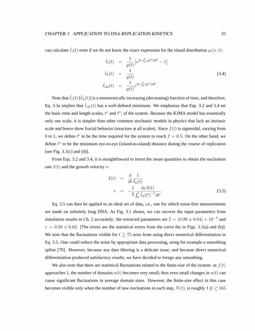
CHAPTER 3. APPLICATION TO DNA REPLICATION KINETICS 35
can calculatei(t) even if we do not know the exact expression for the island distributionρi(x, t):
¯i(t) =
1g(t)
[e2v
R t0 g(t′)dt′ − 1
]¯h(t) =
1g(t)
(3.4)
¯i2i(t) =
1g(t)
e2vR t0 g(t′)dt′ .
Note that i(t) [ ¯h(t)] is a monotonically increasing (decreasing) function of time, and therefore,
Eq. 3.3a implies thati2i(t) has a well-defined minimum. We emphasize that Eqs. 3.2 and 3.4 set
the basic time and length scales,t∗ and`∗, of the system. Because the KJMA model has essentially
only one scale, it is simpler than other common stochastic models in physics that lack an intrinsic
scale and hence show fractal behavior (structure at all scales). Sincef(t) is sigmoidal, varying from
0 to 1, we definet∗ to be the time required for the system to reachf = 0.5. On the other hand, we
define`∗ to be the minimum eye-to-eye (island-to-island) distance during the course of replication
[see Fig. 3.1(c) and (d)].
From Eqs. 3.2 and 3.4, it is straightfoward to invert the mean quantities to obtain the nucleation
rateI(t) and the growth velocityv:
I(t) =d
dt
1¯h(t)
v = −12
lnS(t)∫ t0
¯h(t′)−1
dt′. (3.5)
Eq. 3.5 can then be applied to an ideal set of data, ı.e., one for which noise-free measurements
are made on infinitely long DNA. As Fig. 3.1 shows, we can recover the input parameters from
simulation results in Ch. 2 accurately: the extracted parameters areI = (0.99 ± 0.04) × 10−5 and
v = 0.50 ± 0.02. [The errors are the statistical errors from the curve fits in Figs. 3.1(a) and (b)].
We note that the fluctuations visible fort & 75 arise from using direct numerical differentiation in
Eq. 3.5. One could reduce the noise by appropriate data processing, using for example a smoothing
spline [70]. However, because any data filtering is a delicate issue, and because direct numerical
differentiation produced satisfactory results, we have decided to forego any smoothing.
We also note that there are statistical fluctuations related to the finite-size of the system: asf(t)
approaches 1, the number of domainsn(t) becomes very small; thus even small changes inn(t) can
cause significant fluctuations in average domain sizes. However, the finite-size effect in this case
becomes visible only when the number of new nucleations in each step,N(t), is roughly 1 (t & 165

CHAPTER 3. APPLICATION TO DNA REPLICATION KINETICS 36
(a)
(c) (d)
(b)
1.0
0.5
0.0
isla
nd fr
actio
n150750
time
t*
1.0
0.5
0.0
velo
city
500
0avg.
dom
ain
size
150750time
Hole Eye(Island)
i2il *
0.004
0nucl
eatio
n ra
te
Figure 3.1: Parameter extraction from an almost ideal data set. (a) Inferred nucleation rate vs. time;
(b) Velocity vs. time; (c) Average domain sizes vs. time; (d) Island fraction vs. time; theory and
extractedf(t) overlap. In (c), ∗ is the minimum average eye-to-to spacing, and sets the basic length
scale. In (d),t∗ is the time at which 50% of the genome has replicated. It sets the basic time scale.
or f & 0.999). The effect can be ignored forN(t) � 1 for the practically infinite system considered
here [53, 54].
In the following sections, we consider the complications that arise from less-ideal experimental
conditions.
3.2.2 Asynchrony
As we mentioned above, data often come from experiments where the DNA from many different
independently replicating cells is simultaneously present in the same test tube. The individual DNA
molecules begin replicating at different unknown starting times. In such cases, it is simpler to begin
by sorting data by the replicated fractionf of the measured segment [79]. The basic idea is that,
for spatially homogeneous replication (namely, nucleation and growth), all segments with a similar
fractionf are at roughly the same point in S phase. Sincef(t) is a monotonically increasing function

CHAPTER 3. APPLICATION TO DNA REPLICATION KINETICS 37
of t, we can essentially usef as our initial clock, leaving the conversion to real timet to a second
step.
Once the data have been sorted byf , we extract the initiation frequencyI as a function off .
Using Eqs. 3.2-3.4, one can straightforwardly obtain expressions analogous to Eq. 3.5:
I(f)2v
=1
¯i + ¯
h
d
df
1¯h
2vt(f) =∫ f
0(¯i + ¯
h) df. (3.6)
In Eq. 3.6,¯i and¯h are functions off . In other words, we have a direct inversionI/2v vs. 2vt from
data [Fig. 3.2(a)]. Note that bothI andt are always accompanied by the factor2v, which has to be
determined independently (see below). On the other hand, the fluctuations in the extractedI/2v are
the result of the direct numerical differentiation in Eq. 3.6 discussed in the previous section.
In the two-color labeling experiments, we can compile statistics into histograms of the distri-
bution ρ(f, τi) of replicated fractionsf at time τi [Fig. 3.2(b)], whereτi is the timepoint where
the second dye was added (Fig. 2.1). Note that the spread inρ(f, τi) is related to the starting-time
distributionφ(τ) via the kinetic curvef(t), whereτ is the laboratory time that each DNA starts repli-
cating, andt is the duration of time since the onset of replication. Sinceφ(τ)dτ = ρ(f(t), τi) ·df(t),
wheret = τi − τ , we obtain
ρ(f, τi) = φ(τ)×(
df
dτ
∣∣∣t=τi−τ
)−1
. (3.7)
For a Gaussian starting time distributionφ(τ), one can in principle fit allρ(f, τi)’s using three
fitting parameters,v, the average starting timeτ0, and the starting time widthστ . Unfortunately,
this “brute-force” approach did not produce satisfactory results, as the basin of attraction of the
minimum proved to be relatively small.
Our strategy, then, was first to obtain a coarse-grainedv vs. globalχ2 plot, shown in Fig. 3.2, as
follows:
1. Guess a range ofv betweenvmin andvmax.
2. Fix v (starting fromv = vmin), and traceρ(f, τi) back in time. For a specific value off and
timepointτi, the corresponding starting time isτi − t(f) (Eq. 3.6). Repeat for allρ(f, τi)’s
and reconstruct the starting time distributionφ(t).

CHAPTER 3. APPLICATION TO DNA REPLICATION KINETICS 38
10
0
dist
ribut
ion
80400starting time
18
0
ρ(f,
t i)
1.00.50.0
f
400
0
dom
ain
size
1.00.50.0
f
holeseyes
140700
2vt
1.0
0.5
0.0
f
250 1000 104
0.003
0
I/2v
140700
2vt
250 1000 104(a) (b) (c)
(d) (e) (f)
χ2
0.80.50.2v
Figure 3.2: Inversion results in the presence of asynchrony and finite-size effects. (a)I/2v vs. 2vt.
The arrows indicate wheref = 0.8 in f vs. t curves in (d) for three different molecule sizes:
104 (unchopped), 1000 and 250 (chopped). (b)ρ(f, τi) for six time points 60, 80, 100, 120, 140,
160 (from left to right). The circles are simulation data; the solid lines are from Eq. 3.7, using
the extracted parameters in Table 3.1. (c) Optimization results for the starting-time distribution
φ(τ). The solid line is a Gaussian fit. (d)f vs. 2vt for `c = 250 and`c = 1000. The solid line
is the unchopped case (size104). (e) Average domain sizes vs.f . The empty circles are for the
unchopped case, while the dotted and dashed curves correspond to`c = 1000 and 250. (f) Plot of
log χ2 [ρ(f, τi)] (arbitrary units) vs.v for size104. The complete fit results are shown in Table 3.1.
See also text.
3. Fit φ(τ) obtained in step 1 to an empirical model. [In the absence of correlations among
starting times, a Gaussian distribution is a reasonable choice.2 One may also know the rough
form of φ(τ) from an understanding of the origins of the asynchrony.]
4. Regenerateρ(f, τi) using Eq. 3.7 with the parameters obtained in steps 2 and 3. Calculate
χ2 for ρ(f, τi). This is also a global fit, as theχ2 statistic is summed over data from all time
2Since the only relevant parameters ofφ(τ) are its mean and standard deviation, maximum-entropy arguments also
justify the choice of a Gaussian distribution [80].

CHAPTER 3. APPLICATION TO DNA REPLICATION KINETICS 39
input extracted
I 1× 10⁻⁵ (0.98± 0.18)× 10−5
v 0.5 0.453
startingt (τ0 ± στ ) 39.6± 14.1 36.5± 13.9
Table 3.1: Comparison between input and extracted parameters in the presence of asynchrony (start-
ing t). Note that the inputτ0±στ is the Gaussian fit to a single realization of 1000 molecules, where
τ0 = 40 andστ = 10.6
pointsτi.
5. Increasev to v+∆v and repeat 2–4. If there is a well-defined minimum of theχ2(v) (with
correspondingτ0 and στ ) [e.g., Fig. 3.2(f)], one can find a more accurate estimate of the
minimum using a standard optimization technique such as Brent’s method [70].3 Otherwise,
go back to 1 and choose a different range ofv.
In order to test how well the optimization method described above can work in the face of
asynchrony, we have repeated the simulation in Ch. 2 with several modifications. First, we have
used 1000 molecules that started nucleations asynchronously, following a Gaussian distribution of
average starting timeτ0 = 40 and of starting time widthστ = 10.4 Second, the size of each
individual molecule is104 instead of107. This keeps constant the total number of “DNA basepairs”
analyzed.
Since we used the same nucleation rate, the time to replicate tof = 0.9 was roughly 100
minutes, about the same as for the much larger system [see Fig. 3.1(d) and Fig. 3.2(d)]. We have
chosen six timepoints (τi = 60, 80, 100, 120, 140, 160) at which to collect data, and the distributions
of fractionf are shown in Fig. 3.2(b). The spread inρ(f, τi) reflects the starting time distribution
φ(τ).
We fit I/2v vs. 2vt usingI(t) = a + I · t in Fig. 3.2(a), excluding the last few points roughly
abovef = 0.9 to take into account the finite-size effect (see the following section). We then used the
fit result to obtain the growth ratev by the optimization method given above. The results are shown
3The “Optimize” function in Igor Pro [73] uses Brent’s method.4We note that the actual realization of starting times in the particular simulation of Table 3.1 isτ0 = 39.6 and
στ = 14.1. In other words, there are always errors related to the amount of data used in analysis, but this is a separate
issue from the extraction methods presented here.

CHAPTER 3. APPLICATION TO DNA REPLICATION KINETICS 40
in Fig. 3.2 and Table 3.1. In the plot ofχ2 vs. v [Fig. 3.2(f)], we see a well-defined minimum ofχ2
at v = 0.453, 10% below the input value 0.5. Fig. 3.2(b) and (c) are reconstructions ofρ(f, τi) and
φ(τ) using the parameters in Table 3.1. The minor discrepancies inτ0 andστ are acceptable, given
the small number of points ofρ(f, τi) used in the optimization (20 points in each of six histograms).
Note that the finite size of sampled DNA is responsible for a larger part of the discrepancy with the
original parameters than was our reconstruction algorithm.
The success of this method depends on the experimental design, as well; ı.e., one has to choose
the right timepointsτi in order to deduceφ(τ) accurately [see Fig. 3.2(b) and (c)]. The key parameter
is the ratioα between the replication time scalet∗ and the starting-time widthστ , respectively:
α = t∗/στ . For the case considered here (t∗ ≈ 75 andστ ≈ 14), α ≈ 5.4.
Ideally, α � 1 (better synchrony with slow kinetics), so thatρ(f, τi) has a well-defined peak
between0 < f < 1, andρ(f, τi) → 0 asf → 0 and 1. In this case, even a singleρ(f, τi) can be
used to reconstructφ(τ) and extractv accurately. For example, for all timepoints in Fig. 3.2(b) each
single histogram produced results that are accurate to 15%.
Forα � 1 (high asynchrony with fast kinetics),ρ(f, τi) is spread over0 ≤ f ≤ 1. In this case,
experimentalists should choose at leastN = στ/t∗ timepoints to cover the whole range ofφ(τ),
where well-chosenτi’s spread evenly the peaks ofρ(f, τi) between 0 and 1.
3.2.3 Finite-size effects
As mentioned above, the DNA is broken up into relatively short segments during the molecular-
combing experiments. In order to estimate how the finite segment size affects the estimates ofI(t)
andv, we have cut the simulated molecules in the previous section into smaller pieces of equal size
`c.7 Fig. 3.2 shows results forc = 1000 and 250, with original size104. As one can see, there is
a clear correlation betweenc and the statistics. First, the smaller the segments are, the smaller the
average domain sizes become asf → 1. This is as expected, since one obviously cannot observe
a domain size larger thanc. Note that an underestimate of average eye and hole sizes,¯i and
¯h, leads to an overestimate of the extractedI(t), as implied by Eq. 3.6. Second, as`c becomes
smaller, the completion times are underestimated. Third, the sharp increase (decrease) in average
eye (hole) sizes disappears, becoming nearly flat at a characteristic fractionf∗, and the kinetic curve
7Experimentally, the size distribution of DNA fragments is log normal. See Fig. 4.8. Similar finite-size effects are
obtained for any unimodal distribution with the same mean.

CHAPTER 3. APPLICATION TO DNA REPLICATION KINETICS 41
(a) (b) (c)15
0
I/2v·l*2
210
t/t*
unchopped 1000 250
5
0dom
ain
size
/l*
1.00.50.0
f
unchopped 1000 250
210t/t*
1.0
0.5
0.0
f
unchopped 1000 250
Figure 3.3: Rescaled graphs for finite-size effects (see text). (a)f vs. t/t∗. (b) I2v `2 vs. t/t∗. (c)
`/`∗ vs. f , where` is the average hole (eye) size.
f(t) significantly deviates from its sigmoidal shape, becoming nearly linear. In fact, there is a close
relationship between these last two effects. The sharp increase in average eye size results from the
merger of smaller eyes, which dominates the late stage of replication kinetics. Since chopping DNA
eliminates the large eyes, as shown in Fig. 3.2(e), it effectively increases the number of domains
n(t) per unit length in truncated segments and overestimates the replication rate. (The replication
ratedf/dt = 2vn.)
We emphasize that the first two observations above imply that`c affects the basic time and length
scales,t∗ and`∗, of the (chopped) systems introduced in the previous section. In Figs. 3.3(a)-(c), we
re-plotf(t), I(t), and¯i and ¯
h using the dimensionless axes. One can clearly see that the chopping
process straightens the sigmoidalf(t) and the average domain size curves. Nevertheless, the basic
shape ofI(t) does not change: curves corresponding to different values of`c collapse onto one
another, and the finite-size effect only makes the up-shooting tails steeper.
As criteria for significance of finite-size effects, we first define a new parameterβ = `c/`∗,
namely, the maximum average number of domains per chopped molecule (aroundf = 0.5). Then,
more careful observation of Figs. 3.3(a) and (c) suggests that there might exist a critical valueβ∗ (or
corresponding chopping size`∗c), where the finite-size effects severely affect the statistics. In other
words, forβ > β∗, one can ignore the finite-size effects by excluding the last few data points close
to f = 1 (Recall that ∗ is the minimum average eye-to-eye spacing). To see this clearly, in Fig. 3.4,
we have plottedt∗/t∗∞ vs. β for two different cases:I(t) = 10−5 t andI(t) = 0.001, wheret∗∞
has been calculated using the basic kinetic curvef(t) = 1 − exp[−2v∫ t0 g(t′)dt′] (ı.e., the system
is infinitely large) [77] (see also footnote 1 under Eq. 3.1).
Indeed, changes int∗ are very slow aboveβ ≈ 10, but drop sharply below this ratio. Sinceβ

CHAPTER 3. APPLICATION TO DNA REPLICATION KINETICS 42
1.0
0.5
0.0
t*/ t*∞
200150100500β = lc / l*
I(t) = 10-5 t
I(t) = 0.001
Figure 3.4: The finite-size effects and changes in the basic time and length scales. Shown are two
different initiation ratesI(t) = 10−5t andI(t) = 0.001. The vertical line is where the average
number of domains per molecule is 10. The y-axis has been normalized relative to the initiation rate
for an infinite system (β →∞).
is the average number of domains per molecule, we argue that the KJMA model can be applied to
data directly when there are enough eyes in individual molecule fragments (roughly, at least 10). On
the other hand, whenβ . 10, one would require more sophisticated theoretical methods to obtain
correct statistics.
One subtle point is thatt∗, unlike `∗, is not very accessible experimentally and requires data
processing for accurate extraction [e.g., Fig. 3.2(d) or Fig. 3.5(b)].
Finally, we note that the sudden up-shooting in the tails of the extractedI(t)/2v vs. 2vt curves
is yet another kind of finite-size effect related to numerical differentiation (Eq. 3.5). This can be
simply excluded from the analysis.

CHAPTER 3. APPLICATION TO DNA REPLICATION KINETICS 43
5
0dom
ain
size
/l *
1.00.50.0
f
holes eyes
1.0
0.5
0.0
f
210t/t*
15
0
I/2v·l*2
210
t/t*
raw 1 5
(a) (b) (c)500
0
dom
ain
size
1.00.50.0
f
holeseyes
180120600
2vt
1.0
0.5
0.0
f
1 5
0.003
0
I/2v
180120600
2vt
1
5
(d) (e) (f)
Figure 3.5: The effect of coarse-graining. (a)f vs. 2vt. From left to right,∆x∗ = 0, 1, 5. (b)I/2v
vs. 2vt. From top to bottom, the coarse-graining factor∆x∗ = 0 (no coarse-graining), 1 (comparable
to optical resolution), and 5. (c) Average domain sizes vs.f . The empty circles are for no coarse-
graining, while the dashed lines are for∆x∗ = 1 and 5 (dotted and dashed, respectively). (d)-(f)
Rescaled graphs.
3.2.4 Finite-resolution effect
Another generic problem is the finite resolution of measurements. In molecular-combing experi-
ments, for example, epifluorescence microscopy is used to scan the fluorescent tracks of combed
DNA on glass slides. The spatial resolution (∼1 kb) means that smaller domains will not be de-
tectable. Thus, two eyes separated by a hole of size≤ 1 kb will be falsely assumed to be one longer
eye. We evaluate this effect by coarse-graining the statistics with experimental resolutions∆x∗,
while keeping∆x = v · dt in simulation much finer. To coarse grain by a factorδ = ∆x∗/∆x, we
have used the raw, “unchopped” data set in the previous finite-size-effect section: after the simula-
tion, we have scanned the final lists of eyes and holes,{i} and{h}, and removed any eyes (holes)
for δ < 1, combining them with the two flanking holes (eyes) into a larger hole (eye) that equals the
size of all three domains.

CHAPTER 3. APPLICATION TO DNA REPLICATION KINETICS 44
In Figs. 3.5(a)-(c), we show how the statistics change by coarse-graining only (ı.e., without
chopping), where the coarse-graining factorsδ are 20 and 100.
The finite-resolution effect biases estimates in a way that is opposite to finite-size effects, ı.e.,
converting eyes (holes) forδ < 1 to holes (eyes) increases the average domain sizes. As a conse-
quence, the extractedI(t) is slightly underestimated. Nevertheless, the curves in each off(t), I(t),
and ¯i and ¯
h almost perfectly collapse onto each other when the axes are rescaled usingt∗ and`∗,
confirming that, as with finite-size effects, the main consequence is a change in the basic time and
length scales of the problem [Fig. 3.5(d)-(f)].
To find criteria for significance of finite-resolution effects, we recall that coarse-graining falsely
eliminates eyes and holes smaller than the resolution∆x∗ only (δ < 1). For example, statistics for
f≈0 (small eyes) orf≈1 (small holes) can be affected by coarse-graining. For these two cases,
however, one can easily avoid a problem by excluding data forf ≈ 0 and 1 from analysis.
On the other hand, a more serious situation can arise whenγ = `∗/∆x∗ . 1, because a res-
olution comparable to the minimum eye-to-eye distance will seriously alter the mean domain sizes
¯i and ¯
h and thus the extractedI(t), as well. Indeed, forγ � 1, theρ(f, τi)’s remain essentially
unchanged (ı.e., the optimization result forv remains the same) even atδ = 100 (where,γ ≈ 70)
(data not shown). We conclude thatγ = 1 is the relevant criterion to test the significance of finite-
resolution effects.
3.3 Discussion and Conclusion
In the previous section, we have tested various generic experimental limitations via Monte Carlo
simulation. When the system is large (107 for v = 0.5 andI(t) = 10−5 t), we have been able
to extract all the input parameters accurately from a single realization of our simulation. As the
experimental (simulation) conditions become less ideal, however, one requires more sophisticated
tools.
In the presence of asynchrony, we have demonstrated that the input parameters can still be
extracted to reasonable accuracy (roughly10% for α ≈ 5.4) using an optimization method. In most
DNA replication experiments,α & 1. In this case, the method presented here can even be applied to
dataρ(f, τi) for a single well-chosen timepointτi to extractv. The accuracy increases as more data
are collected for different timepoints. Similarly, the significance of finite-size and finite-resolution
effects can be estimated by the criterionβ = `∗/`c ≈ 10 andγ = `∗/∆x∗ > 1, respectively.

CHAPTER 3. APPLICATION TO DNA REPLICATION KINETICS 45
Among the various experimental limitations we have tested, the finite-size effects seem to be
potentially the most serious problem in the molecular-combing experiments. Fortunately, we expect
the finite-size effects in the experiments and analysis of refs. [44, 59] and in Ch. 4 to be relatively
insignificant becauseβ > 10. On the other hand, we need more sophisticated theoretical tools to
correct the finite-size effects forβ < 10. We recall that the coarse-graining of molecules affects
the tails in Fig. 3.5(b) opposite to the way the finite-size of molecules affects them. We thus spec-
ulate that an intelligent way of annealing finite-sized molecules can reduce or correct the finite-size
effects. We leave a detailed evaluation of this idea for future work.
In summary, we have discussed how to apply the KJMA model to data to extract kinetic param-
eters under various experimental limitations, such as asynchrony, finite-size, and finite-resolution
effects. For the application to DNA-replication experiments, we have shown that finite-size effects
can be ignored when the chopped molecules contain enough domains (ı.e.,β & 10). Even when
the size of molecules is smaller than the critical value`∗c , the shape of the nucleation rateI(t) is
not affected when plotted using rescaled parameters. On the other hand, finite-resolution effects are
insignificant whenγ � 1, which is the case for molecular combing experiments of DNA replication.
In the next chapter, we apply the analysis methods developed here to actual data from recent
experiments on theXenopusegg-extract system.

Chapter 4
Temporal Program of Xenopus
Early-Embryo DNA Replication
4.1 Introduction
In the previous two chapters, we have introduced the KJMA model of nucleation-and-growth and
have extended its 1D version to the case of arbitrary nucleation rateI(t) [77]. We then mapped
DNA replication processes onto the KJMA model and demonstrated that the “kinetic model” can be
used to extract parameters such as the frequency of origin firingsI(t) and fork-growth ratev, which
govern the kinetics of DNA replication [59, 81].
As replicon size and the duration of S phase depend on the values of these parameters, this
information is indispensable for understanding the mechanisms regulating S phase in a given cell
system [36, 82–87]. In other words, understanding how these parameters are coordinated during the
replication of the genome is essential for elucidating the mechanism by which S phase is regulated
in eukaryotic cells. In particular, the extractedI(t) can be interpreted as a “temporal” program of
DNA replication, suggesting a vocabulary that we find useful and intuitive for understanding the
process of replication of various higher eukrayotes from a single unified theoretical framework.
As we shall see, the key feature of recent DNA replication experiments is that they have gathered
much more data than previous experiments could possibly have obtained. In order to appreciate these
advances, we review briefly some of the experimental methods used to analyze DNA replication. For
a more detailed review of classic methods, see the book edited by S. Cotterill [88].
46

CHAPTER 4. TEMPORAL PROGRAM OF XENOPUSDNA REPLICATION 47
In the 1960s, several researchers used autoradiography [60, 89] and electron microscopy [90]
to visualize DNA fibers of lengths ranging fromµm to mm. It soon became obvious that one
can use these visualization techniques to study DNA replication. Indeed, Huberman and Riggs
in 1968 labeled replicating DNA molecules in vivo with3H-thymidine and stretched them out on
filters or microscope slides and then autoradiographed them [91]. Wherever3H-thymidine had
been incorporated into the DNA molecule, a track of silver grains was generated in the overlying
photographic emulsion (sensitive to theβ-particles given off by3H), and the density of silver grains
in those tracks was proportional to the specific activity of the3H-thymidine. Thus, by intentionally
altering the specific activity of the3H-thymidine during an experiment, they could infer the direction
of DNA replication fork movement (as well as measure the fork movement rates and distances
between origins) from the corresponding change in grain density in the final autoradiogram. In
the mean time, electron micrographs were actively used to study DNA replication. In the 1970s, for
example, Kriegstein and Hogness confirmed the bidirectional growth of replication forks [33], while
Blumenthalet al. analyzed spatio-temporal distribution of replication bubbles [79] ofDrosophila
early embryos.
In the 1980s and 1990s, similar but improved techniques were developed, such as the use of
fluorescent molecules instead of radioactive thymidine. An important example is fluorescence in
situ hybridization (FISH) [92, 93]. In this technique, the DNA probe is either labeled directly
by incorporation of a fluorescent-labeled nucleotide precursor, or indirectly by incorporation of a
nucleotide containing a reporter molecule (such as biotin or digoxigenin) which after incorporation
into the DNA is then bound to a fluorescently labeled affinity molecule.
FISH can also be combined with other powerful techniques to achieve high-resolution mapping.
These techniques usually stretch DNA before hybridization. For example, direct visual hybridization
(DIRVISH) involves lysing cells with detergent at one end of a glass slide, tipping the slide, and
allowing the DNA in solution to stream down the slide [24, 25, 94, 95]. The molecular-combing
technique [23] used in theXenopusexperiments of Herricket al. relies on the action of a receding
air/water interface, or meniscus, to uniformly straighten and align DNA molecules on a solid surface
[see Fig. 2.2(d)]. Molecular combing has the advantage not only of producing large quantities of
data but also of reproducibly stretching the DNA at a controlled extension. Thus, there is an accurate
mapping between distances measured on a digital image and lengths along the genome. As explained
in Sec. 2.1, these techniques can produce “snapshots” of replicating DNA that mimic the space-time
diagram in Fig. 2.1. (See Fig. 2.3.)

CHAPTER 4. TEMPORAL PROGRAM OF XENOPUSDNA REPLICATION 48
Although different from the labeling and stretching techniques mentioned above, 2D-gel elec-
trophoresis [96, 97] and DNA microarrays [98–100] have also been important tools to study repli-
cation kinetics, including mapping replication origins. For example, 2D gel electrophoresis allows
the separation of DNA fragments based on both size and shape, thereby separating molecules con-
taining branches in various arrangements (e.g., bubble or Y shapes) from linear molecules. Thus,
by using restriction enzymes that cut DNA at specific sequences, one can map replication origins
using 2D. In particular, the ratio of bubble-shaped molecules to Y-shaped molecules provides a
qualitative estimate of origin efficiency, the relative fraction of cell cycles in which a given origin is
activated [86, 101, 102].
Finally, microarrays containing an ordered set of unique-sequence DNA probes can be used to
monitor DNA replication. They are well-suited for giving information about particular sites along
the genome. For example, in a synchronous population of cells, those genes that have replicated are
twice as abundant as unreplicated genes. One can then identify the position of replication forks by
measuring the abundance of each gene, which is proportional to the amount of DNA that hybridizes
to the array [98]. Similar methods can be extended to construct replication profiles containing
precise locations of replication origins and fork velocities between neighboring origins [99].
These new experimental techniques now make it possible to extract large amounts of data from
the replication process, giving detailed statistics about numbers and sizes of replicated domains as
averaged over the genome, as well as many other related quantities. In particular, in the experiments
by Herrick et al. discussed in this thesis [44], over 200 Mb of DNA replication fragments was
analyzed.
4.2 Results
In this chapter, we apply the KJMA formalism developed in the previous two chapters to recent
experiments on DNA replication in a particular model system ofXenopusegg extracts. Although
our analysis is particular to this system, we stress that it is easily adaptable to experiments on other
systems and experimental data described above.1
Since the kinetics of DNA replication in any cell system depends on two fundamental quantities,
I(t) andv, one of the principal goals of our analysis is to derive accurate values for these quantities,
1This type of model has also been shown to apply for the case of RecA polymerizing on a single molecule of
DNA [103].

CHAPTER 4. TEMPORAL PROGRAM OF XENOPUSDNA REPLICATION 49
including any variation, during the course of S phase.2 The model, as described in the previous
chapters, allows us to draw on a number of previously derived results.
4.2.1 Summary of theXenopusegg extracts replication experiment
Here, we describe recent experimental results obtained on the kinetics of DNA replication in the
well-characterizedXenopus laeviscell-free system [44, 78]. One of the main goals of this chapter
will be to show that, using the theoretical approach described previously, one can extract more
information – more reliably – than before from such experiments.
In theXenopusegg extracts replication experiments, fragments of DNA that have completed one
cycle of replication are stretched out on a glass surface using molecular combing [23, 105, 106]. The
DNA that has replicated prior to some chosen timeτi is labeled with a single fluorescent dye, while
DNA that replicated after that time is labeled with two dyes. The result is a series of samples, each
of which corresponds to a different timet during S phase. Using an optical microscope, one can
directly measure eye, hole, and eye-to-eye lengths at that time. We can thus monitor the evolution
of genome duplication from time point to time point, as DNA synthesis advances. (See Fig. 2.1.)
Cell-free extracts of eggs fromXenopus laevissupport the major transitions of the eukaryotic
cell cycle, including complete chromosome replication under normal cell-cycle control and offers
the opportunity to study the way that DNA replication is coordinated within the cell cycle. In
the experiment, cell extract was added atτ = 2 min, and S phase began 15 to 20 min later. DNA
replication was monitored by incorporating two different fluorescent dyes into the newly synthesized
DNA. The first dye was added before the cell enters S phase in order to label the entire genome. The
second dye was added at successive time pointsτi = 25, 29, 32, 35, 39, and 45 min, in order
to label the later replicating DNA (Fig. 4.1). DNA taken from each time point was combed, and
measurements were made on replicated and unreplicated regions.
The same approach has recently been adapted to study the regulatory parameters of DNA repli-
cation in HeLa cells [95]. Molecular combing, however, has the advantage that a large amount of
DNA may be extended and aligned on a glass slide which ensures significantly better statistics (over
several thousand measurements corresponding to several hundred genomes per coverslip). Indeed,
the molecular-combing experiments provide, for the first time, easy access to the quantities of data
2Althoughv = const. is a good approximation forXenopusearly embyos, in general, the fork velocity can vary greatly
in other eukaryotes depending on the position along the genome [99, 104], and it would be interesting and important to
do new experiments testing this approximation in more detail.
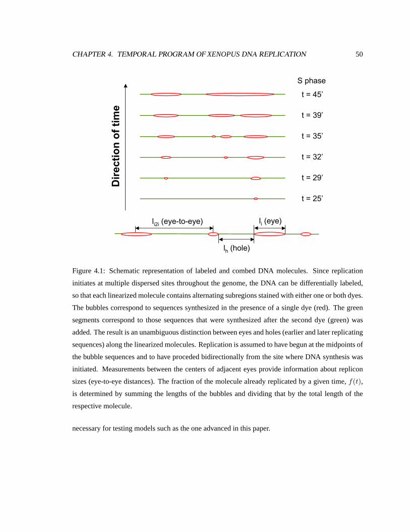
CHAPTER 4. TEMPORAL PROGRAM OF XENOPUSDNA REPLICATION 50
Dir
ecti
on
of
tim
e
li2i (eye-to-eye) li (eye)
lh (hole)
t = 45’
t = 39’
t = 35’
t = 32’
t = 29’
t = 25’
S phase
Figure 4.1: Schematic representation of labeled and combed DNA molecules. Since replication
initiates at multiple dispersed sites throughout the genome, the DNA can be differentially labeled,
so that each linearized molecule contains alternating subregions stained with either one or both dyes.
The bubbles correspond to sequences synthesized in the presence of a single dye (red). The green
segments correspond to those sequences that were synthesized after the second dye (green) was
added. The result is an unambiguous distinction between eyes and holes (earlier and later replicating
sequences) along the linearized molecules. Replication is assumed to have begun at the midpoints of
the bubble sequences and to have proceded bidirectionally from the site where DNA synthesis was
initiated. Measurements between the centers of adjacent eyes provide information about replicon
sizes (eye-to-eye distances). The fraction of the molecule already replicated by a given time,f(t),
is determined by summing the lengths of the bubbles and dividing that by the total length of the
respective molecule.
necessary for testing models such as the one advanced in this paper.

CHAPTER 4. TEMPORAL PROGRAM OF XENOPUSDNA REPLICATION 51
4.2.2 Generalization of the model to account for specific features of theX. laevisex-
periment
The experimental results obtained on the kinetics of DNA replication in thein vitro cell-free system
of Xenopus laevis[44, 78] were analyzed using the kinetic model developed in the previous chap-
ters. In formulating that model, we had to take into account explicitly a number of experimental
limitations discussed in the previous chapter:
1) One goal of the experiment is to measure the initiation functionI(t), which is the probability of
initiating an origin per unit length of unreplicated DNA after time intervalt since the onset of repli-
cation. The simplest assumptions, in terms of our model, would be that eitherI is peaked at or near
t = 0 (all origins initiated at the beginning of S phase) orI(t) = const., (origins initiated at constant
rate throughout S phase). However, neither assumption turns out to be consistent with the data ana-
lyzed here; thus, we formulated our model to allow for arbitrary initiation patterns and deduced an
estimate forI(t) directly from the data. We note that initiation is believed to occur synchronously
during the first half of S phase inDrosophila melanogasterearly embryos [79, 85]. Initiation in the
myxomycetePhysarum polycephalum,on the other hand, occurs in a very broad temporal window,
suggesting that initiation occurs continuously throughout S phase [58]. Finally, recent observations
suggest that, inXenopus laevis, early embryos nucleation may occur with increasing frequency as
DNA synthesis advances [24, 44, 78]. By choosing an appropriate form forI(t), one can account for
any of these scenarios. Below, we show how measured quantities may, using the model, be inverted
to provide an estimate forI(t).
2) The basic form of the model assumes implicitly that the DNA analyzed began replication at “lab-
oratory time”τ = 0, but this may not be so, for two reasons:
i) In the experimental protocols, the DNA analyzed comes from approximately 20,000 indepen-
dently replicating nuclei. Before each genome can replicate, its nuclear membrane must form, along
with, presumably, the replication factories. This process takes 15-20 minutes [107–109]. Because
the exact amount of time can vary from cell to cell, the DNA analyzed at timeτi in the laboratory
may have started replicating over a relatively wide range of times.

CHAPTER 4. TEMPORAL PROGRAM OF XENOPUSDNA REPLICATION 52
ii) In eukaryotic organisms, origin activation may be distributed in a programmed manner through-
out the length of S phase, and, as a consequence, each origin is turned on at a specific time (early
and late) [110].
In the current experiment, the lack of information about the locations of the measured DNA seg-
ments along the genome means that we cannot distinguish between asynchrony due to reasons (i)
or (ii). We have thus accounted for their combined effects using the starting-time distributionφ(τ)
introduced in Ch. 3, which is the probability—for whatever reason—that a given piece of analyzed
DNA began replicating at timeτ in the lab.
3) The combed DNA is broken down into relatively short segments (100-300 kb, typically). Also,
the experiments are all analyzed using an epifluorescence microscope to visualize the fluorescent
tracks of combed DNA on glass slides (with spatial resolution≈ 0.3µm). Thus, we have to estimate
β = `c/`∗ andγ = `∗/∆x∗ for these effects. (See Sec. 3.2.3.)
4.2.3 Application of the kinetic model to the analysis of DNA replication inX. Laevis
Using the generalizations discussed above, we analyzed recent results obtained on DNA replication
in the Xenopus laeviscell-free system. DNA taken from each time point was combed, and mea-
surements were made on replicated and unreplicated regions. Statistics from each time point were
then compiled into six histograms (one for each time point) of the distributionρ(f, τi) of replicated
fractionsf at lab timeτi (Fig. 4.2).
One can immediately see from Fig. 4.2 the need to account for the spread in starting times.
If all the segments of DNA that were analyzed had started replicating at the same time, then the
distributions would have been concentrated over a very small range off . But, as one can see in
Fig. 4.2(c), some segments of DNA (within the same time point) have already finished replicating
(f = 1) before others have even started (f = 0). This spread is far larger than would be expected on
account of the finite length of the segments analyzed. Because of the need to account for the spread
in starting times, it is simpler to begin by sorting data by the replicated fractionf of the measured
segment. We thus assume that all segments with a similar fractionf are at roughly the same point
in S phase, an assumption that we can check by partitioning the data into subsets and redoing our

CHAPTER 4. TEMPORAL PROGRAM OF XENOPUSDNA REPLICATION 53
16
12
8
4
0
1.00.80.60.40.20.0
45 min6
4
2
0
1.00.80.60.40.20.0
39 min6
4
2
0
1.00.80.60.40.20.0
35 min
6
4
2
0
1.00.80.60.40.20.0
32 min6
4
2
0
1.00.80.60.40.20.0
29 min
16
12
8
4
0
Pro
babi
lity
Den
sity
1.00.80.60.40.20.0Fraction Replicated (f)
experimentsimulation theory
25 min
(a) (b) (c)
(d) (e) (f)
Figure 4.2: ρ(f, τi) distributions for the six time points. The curves show the probability that a
molecule at a given time point (a)-(f) has undergone a certain amount of replication before the
second dye was added. The filled circles represent the experimental data. The results of the Monte
Carlo simulation are shown in open circles; analytical curves are the global fitting.
measurements on the subsets. In Fig. 4.3(a)-(c), we plot the mean values`h, `i, and`i2i againstf .
We then findf(t), I(t), and the cumulative distribution of lengths between activated origins of
replication,Itot(t). (See Fig. 4.4.) The direct inversion forI(t) [Fig. 4.4(b)] shows several surpris-
ing features: First, origin activation takes place throughout S phase and with increasing probability
(measured relative to the amount of unreplicated DNA), as recently inferred from a cruder analysis
of data from the same system using plasmid DNA [78]. Second, about halfway through S phase,
there is a marked increase in initiation rate, an observation that, if confirmed, would have biolog-
ical significance. It is not known what might cause a sudden increase (break point) in initiation
frequency halfway through S phase. The increase could reflect a change in chromatin structure that
may occur after a given fraction of the genome has undergone replication. This in turn may increase
the number of potential origins as DNA synthesis advances [111].
The smooth curves in Fig 4.3(a)-(c) are fits based on the model, using anI(t) that has two
linearly increasing regions, with arbitrary slopes and “break point” (three free parameters). The fits

CHAPTER 4. TEMPORAL PROGRAM OF XENOPUSDNA REPLICATION 54
80
60
40
20
0
<E
ye L
engt
h> (
kb)
1.00.80.60.40.20.0
Fraction Replicated (f)
80
60
40
20
0
<H
ole
Leng
th>
(kb
)
1.00.80.60.40.20.0
Fraction Replicated (f)
experiment simulation theory
80
60
40
20
0<E
ye-t
o-E
ye L
engt
h> (
kb)
1.00.80.60.40.20.0
Fraction Replicated (f)
0.1
2
4
1
2
4
10
2
4
100
Leng
th (
kb)
1.00.80.60.40.20.0Fraction Replicated (f)
holes eyes eye-to-eye lengths
(a) (b)
(c) (d)
Figure 4.3: Mean quantities vs. replication fraction. (a) average hole size`h(f); (b) average eye size
`i(f); (c) average eye-to-eye size`i2i(f). Filled circles are data; open circles are from the Monte
Carlo simulation; the solid curve is a least-squares fit, based on a two-segmentI(t); (d) curves in
(a)-(c) collapsed onto a single plot, confirming the mean-field relations (Eqs. 3.3a and 3.3b). (The
discrepancies nearf = 0 and1 reflect measurement errors. Very small eyes or holes may be missed
because of limited optical resolution; very large eyes or holes may be eliminated because of finite
segment sizes.)
are quite good, except where the finite size of the combed DNA fragments becomes relevant. For
example, when mean hole, eye, and eye-to-eye lengths exceed about 10% of the mean fragment
size, larger segments in the distribution for`h(f), etc., are excluded and the averages are biased
down. These biases due to finite sizes of the molecules also affect the last few points in the extracted
I(t) (see below). We confirmed this with the Monte Carlo simulations, the results of which are
overlaid on the experimental data. The finite fragment size in the simulation matches that of the

CHAPTER 4. TEMPORAL PROGRAM OF XENOPUSDNA REPLICATION 55
0.20
0.15
0.10
0.05
0.00Cum
. ini
t. de
nsity
(/k
b)
3020100
Elapsed time tau (min)
0.10
0.08
0.06
0.04
0.02
0.00Initi
atio
n ra
te (
/kb·
min
)
3020100
Elapsed time tau (min)
(a) (b) (c)
1.0
0.8
0.6
0.4
0.2
0.0Fra
ctio
n re
plic
ated
(f)
3020100
Elapsed time tau (min)
data theory
I(t) Itot (t)
Figure 4.4: (a) Fraction of replication completed,f(t). The points are derived from the measure-
ments of mean hole, eye, and eye-to-eye lengths. The curve is an analytic fit (see below). (b)
Initiation rateI(t). The large statistical scatter arises because the data points are obtained by taking
two numerical derivatives of thef(t) points in (c). The last several points are artifacts due to finite-
size effects and were not included in the analysis. (c) Integrated origin separation,Itot(t), which
gives the average distance between all origins activated up to timet. In (a)-(c), the black curves are
from fits that assume thatI(t) has two linear regimes of different slopes. The form we chose forI(t)
was the simplest analytic form consistent with the data in (b). The parameters for the least-squares
fits (slopesI1 andI2, break pointt1) are obtained from a global fit to the eight data sets in Fig.
4.2(a)-(f) and Fig. 4.3(a)-(b), ı.e.,ρ(f) from six time points, h(f), and`i(f).
experiment, leading to the same downward bias. (See, also, Sec. 3.2.3) In Fig. 4.4, we overlay the
fits on the experimental data. We emphasize that we obtainI(t) directly from the data, with no
fit parameters, apart from an overall scaling of the time axis. The analytical form is just a model
that summarizes the main features of the origin-initiation rate we determine via our model, from the
experimental data. We note that the last few points in Fig. 4.4(b) were excluded in the analysis for
reasons explained above.3 The important result isI(t). From the maximum ofItot(t), we find a
mean spacing between activated origins of 6.3± 0.3 kb, which is much smaller than the minimum
3To justify this, we first simulated longer molecules and then created a series of data sets by chopping the longer
molecules. We observed that, as the chopped molecules become smaller, the downward bias in the extractedI(t) becomes
more visible and similar to the one in Fig. 4.4(b). The downward bias observed here results from a different choice of
algorithm for extractingI(t) than was used in Ch. 3. In that chapter, we used Eq. 3.5, while, in this chapter, we used
I(t) = − 12v
d2
dt2ln[1− f(t)]. These two methods are identical for ideal systems, but they can lead to different biases (for
example, upward and downward) in the presence of finite-size effects.

CHAPTER 4. TEMPORAL PROGRAM OF XENOPUSDNA REPLICATION 56
0.10
0.05
0.00
Pro
babi
lity
Den
sity
3020100
Starting Time (min)
data fit
Figure 4.5: Starting-time distributionφ(τ). Solid curve is a least-squares fit to a Gaussian distribu-
tion.
mean eye-to-eye separation 14.4± 1.5 kb.
In our model, the two quantities differ if initiation takes place throughout S phase, as coales-
cence of replicated regions leads to fewer domains, and hence fewer inferred origins.4 The mean
eye-to-eye separation is of particular interest because its inverse is just the domain density (num-
ber of active domains per length), which can be used to estimate the number of active replication
forks at each moment during S phase. For example, the saturation value ofItot corresponds to the
maximum number (about 480,000/genome) of active origins of replication. Since there are about
400 replication foci/cell nucleus, this would indicate a partitioning of approximately 1,200 origins
(or, equivalently, about 7.5 Mb) per replication focus [107, 112]. The distribution off values in
4The minimum average eye-to-eye size is obtained by differentiating¯i2i(t) = 1
g(t)e2v
Rg(t′)·dt′ , whereg(t) =R t
0I(t)dt. For a constant initiation rateI(t) = I0, one obtains ∗
i2i =√
2e ·p
v/I0. Also, we recall¯i2i(t) =
¯i(t) + ¯
h(t) =¯h(t)1−f
, which allows one to collapse the experimental observations of all three mean curves onto a single
one [see Eq. 3.4 and Fig. 4.3(d)].

CHAPTER 4. TEMPORAL PROGRAM OF XENOPUSDNA REPLICATION 57
the ρ(f, τi) plots can be used to deduce the starting-time distribution [φ(τ)], along with the fork
velocity v (see Sec. 3.2.2). (Fig. 4.5). The spread in starting timesφ is consistent with a Gaussian
distribution, with a mean of15.9± 0.6 min. and a standard deviation of6.1± 0.6 min. For the fork
velocity, we findv = 615± 35 bases/min., in excellent agreement with previous estimates∼ 600
bases/min [113, 114]. As with thef data, we extractedφ(τ) andv from a global fit to data from all
six time points.
4.3 Discussion
4.3.1 Initiation throughout S phase
The view that we are led to here, of random initiation events occurring continuously during the
replication ofXenopussperm chromatin in egg extracts, is in striking contrast to what has until re-
cently been the accepted view of a regular periodic organization of replication origins throughout
the genome [83, 84, 115, 116]. For a discussion of experiments that raise doubts on such a view, see
Berezney [104]. The application of our model to the results of Herricket al. indicates that the kinet-
ics of DNA replication in theX. laevis in vitrosystem closely resembles that of genome duplication
in early embryos. Specifically, we find that the time required to duplicate the genomein vitro agrees
well with what is observedin vivo. In addition, the model yields accurate values for replicon sizes
and replication fork velocities that confirm previous observations [36, 113]. Though replicationin
vitro may differ biologically from what occursin vivo, the results nevertheless demonstrate that the
kinetics remains essentially the same. Of course, the specific finding of an increasing rate of ini-
tiation invites a biological interpretation involving a kind of autocatalysis, whereby the replication
process itself leads to the release of a factor whose concentration determines the rate of initiation.
This will be explored in future work.
4.3.2 Asynchrony, finite-size, and finite-resolution effects
In Ch. 3, we introduced various parameters to estimate the significance of experimental limitations
in applying the kinetic model to data. In the data by Herricket al. used here for analysis, all
three effects – asynchrony, finite-size, finite-resolution – are present. Fortunately, we have found
that the asynchrony is well-described by the Gaussian starting-time distributionφ(τ). In this case,
α = t∗/στ ≈ 2.5 (for the duration of S phaset∗ ≈ 15 mins. and the starting-time widthστ of 6.1

CHAPTER 4. TEMPORAL PROGRAM OF XENOPUSDNA REPLICATION 58
Effect Parameter Definition when significant? in Xenopusexpt.
asynchrony α t∗/στ � 1 2.5
finite size β `∗/`c < 10 7-20
finite resolution γ `∗/∆x∗ < 1 10-100
Table 4.1: Summary table concerning the important parameters for experimental limitations.
mins), and the optimization method presented in Ch. 3 can be applied to the data to extractv from
ρ(f, τi) accurately.
On the other hand, the significance of finite-size effects can be estimated by the criterionβ =
`∗/`c ≈ 10. In our case,∗ for Xenopussperm chromatin is roughly 15 kb, while the typical size of
combed molecules ranges between 100 - 300 kb, thus giving7 . β . 20 and making the finite-size
effects relatively insignificant. However, we note that the origin spacing of many higher eukaryotes,
includingXenopusafter the mid-blastula transition, can be as large as 100 kb. In such cases, it is of
critical importance to obtain long combed molecules (> 1 Mb).
Similarly, finite-resolution effects are insignificant whenγ = `∗/∆x∗ > 1. This condition is
satisfied in almost all molecular-combing experiments of DNA replication, since∆x∗ ≈ 1 kb while
`∗ typically ranges between 10 and 100 kb (γ ≈ 10 to 100).
In Table. 4.1, we present a summary showing the relative importance of these “real-world”
effects.
4.3.3 Directions for future experiments inX. laevis
One effect that we did not include in our analysis is a variable fork velocity. For example,v might
decrease as forks coalesce or as replication factor becomes limiting toward the end of S phase [107–
109].
Another important question is to separate the effects of any intrinsic distribution due to early
and late-replicating regions of the genome of a single cell from the extrinsic distribution caused by
having many cells in the experiment. One approach would be to isolate and comb the DNA from a
singlecell. Although difficult, such an experiment is technically feasible. The latter problem could
be resolved byin situfluorescence observations of the chosen cell.

CHAPTER 4. TEMPORAL PROGRAM OF XENOPUSDNA REPLICATION 59
4.3.4 Applications to other systems
One can entertain many further applications of the basic model discussed above, which can be
generalized, if need be. For example, Blumenthalet al. interpreted their results on replication in
Drosophila melanogasterfor ρi2i(`, f) to imply periodically spaced origins in the genome [79]. (See
their Fig. 7.) It is difficult to judge whether their peaks are real or only a statistical happenstance;
but, if the conclusion is indeed that the origins in that system are arranged periodically, the kinetics
model could be generalized in a straightforward way (by introducing anI(x, τ) that was periodic in
x).
Very recently, detailed data on the replication of budding yeast (Saccharomyces cerevisiae) have
become available [99]. The data provide information on the locations of origins and the timings of
their initiation during S phase. These data support the view of origin initiation throughout S phase.
Unlike replication inXenopusprior to the mid-blastula transition, origins in budding yeast are as-
sociated with highly conserved sequence elements (autonomous replication sequence elements, or
ARSs). Raghuramanet al. [99] also give the first estimates of thedistributionof fork velocities dur-
ing replication. Although broad, the distribution is apparently stationary, and there is no correlation
between velocities and the time in S phase when the forks are initiated. The model developed here
could be generalized in a straightforward way to the case of budding yeast. Knowing the sequence
of the genome and hence the location of potential origins means that the initiation function would be
an explicit function of positionx along the genome, with peaks of varying heights at each potential
origin. The advantage of the kind of modeling advanced here would be the opportunity to derive
quantities such as the replication fraction as a function of time in S phase. Raghuramanet al. fit their
data for this “timing curve” to an arbitrarily chosen sigmoidal function. (See their supplementary
data, Section II-5.) Such modeling will make it easier to find meaningful biological explanations of
the programming of S phase evolution.
4.3.5 The random-completion problem: part I
One outstanding issue in DNA replication in eukaryotes is the observation that the replication origins
cannot be too far apart, as this would prevent the genome from being replicated completely within
the length of a single S phase [117]. In the case ofXenopus early-embryo replications, most
solutions suggested so far to prevent the formation fatal long origin spacings concern the density
and the distribution of pre-replication complexes (pre-RCs) of highly conserved proteins, which

CHAPTER 4. TEMPORAL PROGRAM OF XENOPUSDNA REPLICATION 60
not proven, that MCMs form the eukaryotic DNA replication
fork helicase.(9) The recruitment of the MCM2-7 complex at
origins (called replication ‘‘licensing’’) takes place during late
mitosis and the G1 phase, in preparation for the next round of
chromosomeduplication. Licensing strictly requires a complex
of six proteins first identified in budding yeast, the origin
recognition complex (ORC).(10) In yeast, ORC binds replica-
tion origins directly and stably across the cell cycle.(11) In
metazoa, the stability of chromatin association of ORC is
higher at the G1/S transition.(12) Origin licensing also requires
CDC6 and CDT1, which must both interact with ORC to load
MCM2-7 onto chromatin.(13–15) Importantly, once MCM2-7
have been loaded, ORC and probably CDC6 and CDT1
become dispensable for subsequent replication.(14,16,17)
Once loaded, MCM2-7 complexes await activation during
S phase. This process is triggered by at least two kinases,
CDC7/DBF4 and the S-CDKs, and involves the ordered
assembly of additional proteins, among which CDC45 has
emerged as a pivotal factor.(1) CDC45 origin association
triggers origin DNA unwinding and ultimately leads to the
association of DNA polymerases with the unwound DNA
(Fig. 1).(18,19) In yeast, MCM2-7 dissociate from origins either
upon replication initiation(20,21) or upon passive replication
from a neighboring origin.(22,23) Biochemical and immuno-
fluorescence studies in metazoan cells also suggest that
MCMs are progressively excluded from replicated chromatin
during S phase.(24–29) The reloading of MCMs is prevented
until cells pass throughmitosis byCDKsandbygeminin.CDKs
interfere with various functions of ORC, CDC6 and MCMs in
licensing.(30) Geminin (only found in metazoa) binds and
inhibitsCDT1.(31,32) Cyclins (and thereforeCDKactivities) and
geminin are only destroyed in latemitosis, ensuring that a new
round of origin licensing can only take place after sister
chromatid segregation. The strict temporal separation ofMCM
loading and activation and the release of MCMs from repli-
cated DNA ensure that no sequence is replicated more than
once in a single S phase.
Although several lines of evidence argue that the MCMs
form the replicative DNA helicase, some observations are not
easily explained by this model. First, immunofluorescence
studies in mammalian cells(26–28) and in frog egg extracts(29)
show that, in contrast to bona fide replication fork proteins such
as RP-A and PCNA, which colocalize with newly replicated
DNA, most of the MCMs colocalize with unreplicated DNA.
One study showed a lack of co-localization of MCMs directly
with RP-A and PCNA, or with DNA synthesized during the
period preceding fixation.(26) Second, chromatin immunopre-
cipitation experiments suggest that ORC and MCMs do not
resideonclosely adjacent sites inmammalian chromatin, even
in cells arrested at the G1/S boundary.(33) Finally, the number
of chromatin-bound MCM complexes exceeds the number of
replication origins and ORC complexes by a factor of 10–100
in various organisms. The ‘‘MCM paradox’’(26) is that MCM
proteins are in vast excess and do not colocalize with
replication forks.
Dispersive versus site-specific initiation
While replication initiation proteins are widely conserved,
replication origins are not.(34) In S. cerevisiae, specific se-
quences that can promote autonomous plasmid replication
(autonomously replicating sequences; ARSs) define the sites
where the synthesis of new DNA strands starts both on
plasmids and within yeast chromosomes.(35) Genomic foot-
printing indicates that ARSsare stably boundbyORC through-
out the cell cycle(11) and that, during latemitosis andG1 phase,
MCM2-7 bind alongside ORC to form a larger prereplicative
complex (pre-RC).(36) High-resolution mapping has shown
that replication initiates precisely at the center of the pre-RC
footprint for one ARS.(37)
In contrast to yeast, attempts to isolate specific sequences
that provide autonomous replication to transfected plasmids
in animal cells have been inconclusive.(34) In one study with
human cells, any sequence appeared suitable provided it is
large enough (>10 kb),(38) and replication was found to initiate
at multiple, apparently random sites on the plasmid.(39)
Physical mapping of chromosomal origins in adult animal cells
has given more complex results. At loci such as the human
lamin B2(40) and b-globin(41) genes, replication initiates at
Figure 1. Licensing and activation of replication
origins.MCM2-7are loadedduring latemitosis and
G1 phase onto replication origins by ORC, CDT1
and CDC6 (origin licensing). Pre-replication com-
plexes (Pre-RC) are activated at the G1/S transi-
tion by two kinases, CDC7/DBF4 and S-CDKs.
A key step in this transition to replication is the
recruitment of CDC45. MCM2-7 dissociate from
DNA as S phase progresses. Reloading of MCM2-
7 is prevented by at least two inhibitors, geminin
and the CDKs. This inhibition persists until cells
pass through mitosis, when geminin and cyclins
are destroyed.
Review articles
BioEssays 25.2 117
Figure 4.6: Licensing and activation of replication origins. MCM2-7 complexes, proteins that are
believed to be competent to initiate replication, are loaded during late mitosis and G1 phase onto
replication origins by ORC, CDT1, and CDC6 (origin licensing). Pre-replication complexes (pre-
RC) are activated at the G1/S transition by two kinases, CDC7/DBF4 and S-CDKs. A key step in
this transition to replication is the recruitment of CDC45. MCM2-7 dissociate from DNA as S phase
progresses. Reloading of MCM2-7 is prevented by at least two inhibitors, geminin and the CDKs.
This inhibition persists until cells pass through mitosis, when geminin and cyclins are destroyed.
Figure and caption from Ref. [35] by O. Hyrien. Copyrightc©2003 Wiley-Liss, Inc., a subsidiary of
John Wiley & Sons, Inc. Reprinted by permission of John Wiley & Sons, Inc.
assemble at ORC-bound DNA sites before the cell enters S phase (Fig. 4.6) [35].
For example, one solution that has been proposed is that there is an excess of pre-RCs (e.g.,
Lucaset al. [78], and references therein). In this case, the position of each potential origin of
replication (POR) can be distributed randomly, with a statistically insignificant probability of having
large gaps between PORs. The problem with this solution has been that the average POR spacing
must be much smaller (less than 1-2 kb) than the reported 7-16 kb spacings ofXenopus ORC
(XORC), protein complex that has been believed to be directly associated with PORs until recently
[82, 118],
A second proposed solution to the random-completion problem is to invoke correlations in POR
spacings. In other words, instead of assuming a purely random pre-RC distribution, one imposes
constraints that force a partial periodicity on the POR spacing, so that most of the origins are spaced
5-15 kb apart (Blow et al. [24] and references therein). This suppresses the formation of large gaps
but raises other issues. First, it requires an unknown mechanism to achieve this periodicity of POR

CHAPTER 4. TEMPORAL PROGRAM OF XENOPUSDNA REPLICATION 61
Fig 6
5
0
Prob
abilit
y de
nsity
1.00.50.0
Relative position in holes
holes > 22 kbExperimentSim (random)Sim (loop)
5
0
Prob
abilit
y de
nsity
1.00.50.0
Relative position in holes
8 kb < holes < 22 kb(a) (b)
Prob
abilit
y de
nsity
Prob
abilit
y de
nsity
Relative position in holes Relative position in holes
8 kb < holes < 22 kb 22 kb < holes
Figure 4.7: (a) Histogram of positions of initiation events for holes 8-22 kb in size. The events are
determined by looking for replicated domains that are small enough that they very likely contain only
a single replication origin. The state of the molecular fragment is then propagated back in time to
the moment of initiation, where one records the hole size and relative position of the initiation event
within the hole. The inset shows a hole flanked by two eyes. The experimental histogram shows
that it is more likely that a new initiation occurs near the center of a hole, an observation compatible
with the looping scenario but not with the purely random initiation scenario. (b) Holes larger than
22 kb. The difference between experiment and simulations (both random and loop formation) is
much smaller than for small holes in (a).
spacing. Second, it assumes implicitly that most of the PORs fire during S phase, to prevent the 30
kb gap that could arise from a origin’s failure to initiate. Blow’s model is thus not robust in that
the failure of a single origin to initiate could double the time needed complete replication. Third, if
origins initiate throughout S phase, then there needs to be some kind of correlation that forces the
more widely spaced origin groups to initiate early enough in S phase to complete replication in the
required time.
Implicitly, our model adopts language consistent with the first solution, but it is straightforward
to consider the correlations assumed in the second solution. The presence of significant correlations
in PORs would not invalidate the results presented here, which pertain to mean quantities (e.g.,
Fig. 4.3); however, it would change their interpretation and could change biological models that one
might try to make to explain the observed kinetic parameters we extract using the KJMA model.
Indeed, the resolution of the origin-spacing problem in early embryos requires not only the temporal

CHAPTER 4. TEMPORAL PROGRAM OF XENOPUSDNA REPLICATION 62
[I(t)] but also “spatial” program of DNA replication, and our data also suggest that initiation of
replication origins is not spatially homogeneous. As an example, Fig. 4.7 shows histograms that
record the relative position of new origins within a hole. In Fig. 4.7(a), we plot the distribution for
small holes, 8-22 kb in length.5 The experimental data shows a strong peak near 0.5, implying a
tendency for origins to be as far away from other replicating domains as possible. By contrast, the
experimental data for large holes shows a much more uniform distribution. In simulations that use
spatially homogeneous initiation, new origins can appear almost anywhere in a hole, regardless of
its size. This picture fits the large-hole data [Fig. 4.7(b)] but not the small-hole data [Fig. 4.7(a)]. By
contrast, when we put in the effects of suppression of origin initiation by chromatin looping at very
close spacings and an enhancement of initiation at a larger, characteristic distance, the simulation
results match more closely the data of Fig. 4.7(a), while continuing to agree with the large-hole case.
In the next chapter (Sec. 5.3.2), we shall explain how the origin-spacing problem (or, the “random-
completion” problem) can be solved by understanding the physical properties of chromatin and its
looping.
4.4 Conclusion
So far, we have introduced a class of theoretical models for describing replication kinetics that is
inspired by well-known models of crystal-growth kinetics. The model allows us to extract the rate
of initiation of new origins, a quantity whose time dependence has not previously been measured.
With remarkably few parameters, the model fits quantitatively the most detailed existing experiment
on replication inXenopus. It reproduces known results (for example, the fork velocity) and provides
the first reliable description of the temporal organization of replication initiation in a higher eukary-
ote. Perhaps most important, the model can be generalized in a straightforward way to describe
replication and extract relevant parameters in essentially any organism.
5Holes smaller than 8 kb in length showed a bias toward the center in the experimental data and were not included for
comparison to models lacking such bias.

CHAPTER 4. TEMPORAL PROGRAM OF XENOPUSDNA REPLICATION 63
0.01
0
Pro
babi
lity
dens
ity
5004003002001000
DNA length (kb)
Figure 4.8: Distribution of combed DNA molecules used in the analysis: the average length was 102
kb and the standard deviation 75 kb. The distribution is approximately log normal.
4.5 Appendix
4.5.1 Monte Carlo simulations
We wrote a Monte Carlo simulation using the programming language of Igor Pro [73] to test various
experimental effects that were difficult to model analytically. As we discussed in Ch. 3, these in-
cluded the effects of finite sampling of DNA fragments (on average, 190 molecules per time point),
the finite optical resolution of the scanned images, and – most important – the effect of the finite
size of the combed DNA fragments. The size of each molecular fragment in the simulation was
drawn randomly from an estimate of the actual size distribution of the experimental data (Fig. 4.8).
This distribution was approximately log-normal, with an average length of 102 kb and a standard
deviation of 75 kb.
We used both the lattice model and a variation of the double-list algorithm for our simulations
(see Ch. 2). The timestep∆t = 0.2 min, and the lattice sizev∆t = 123 bp for the measured fork
velocity v = 615 bp/min. The lattice scale is then roughly the size of origin recognition complex
proteins. We sampled the simulation results at the same time points as the actual experiments (τi
= 25, 29, 32, 35, 39, 45 minutes). Each sampled molecule is cut at random site to simulate the

CHAPTER 4. TEMPORAL PROGRAM OF XENOPUSDNA REPLICATION 64
combing process. The lattice is then “coarse grained” by averaging over approximately four pixels.
The coarse lattice length scale is then 0.24µm, which roughly corresponds to the resolution of the
scanned optical images. Finally, the coarse-grained fragments were analyzed to compile statistics
concerning replicon sizes, eye-to-eye sizes, etc. that were directly compared to experimental data.
We also used the simulation to test a previous algorithm for extractingI(f), the initiation rate as
a function of overall replication fraction. The previous algorithm [44, 119] looked for small repli-
cated regions and extrapolated back to an assumed initiation time. The effects of eye coalescence is
not taken into account. We tested this algorithm using our Monte Carlo analysis and, as expected,
found significant bias in the inferredI(f), while the algorithms we introduce here showed no such
bias.
4.5.2 Parameter extraction from data and experimental limitations
We extracted data from both the real experiments and the Monte Carlo simulations by a global
least-squares fit that took into account simultaneously the different data collected (ı.e., the different
curves in Figs. 4.2 and 4.3). As discussed above, we fit a two-segment straight line to theI(t) curve
extracted directly from the data for analytic simplicity. Assuming this form forI(t), we derive
explicit formulae for the curves in Figs. 4.2 and 4.3.
The finite size of the molecular fragments studied (102±75 kb) causes systematic deviation from
the “infinite-length” formulae. Such deviations could be detected using the Monte Carlo simulations
by comparing the extracted values of parameters with those input. The deviations show themselves
mainly in two settings: First, whenever the mean length of holes, eyes, or eye-to-eye distances
approaches the mean segment length, the observed mean lengths will be systematically too small
because the larger end of the experimental distributions is cut off by the finite fragment length. We
dealt with this complication by restricting our fit to areas where the mean length being measured is
less than 10% of the mean fragment size. The second complication is that the inferred fork velocity
is systematically reduced (by about 5% for the fragment size in the experiments analyzed here). We
measured this bias using the Monte Carlo simulations and then corrected the “raw” fork velocity that
is given by our least-squares fits. Fortunately, these corrections are expected to be minor because
the data we used satisfies the conditionβ & 10. For further details, see Sec. 3.2.3.
One further subtle point in a global fit is the relative weighting to be given to the data in theρ(f)
curves (Fig. 4.2) relative to the data in the mean-value curves (Fig. 4.3). We estimated the weights

CHAPTER 4. TEMPORAL PROGRAM OF XENOPUSDNA REPLICATION 65
using the boot-strap method [70]. The basic idea is to createM sets of data by randomly drawing
data points from the original set. In other words, each created data set will consist of the same
number of data points as the original one, but it now has a random fraction of the original points,
typically ∼ 1/e ≈ 37%. One then analyzes the artificial data sets as data fromM independent
experiments. In a similar spirit, we used repeated Monte Carlo simulations to estimate statistical
errors in experimentally extracted quantities, ı.e., we used our simulation to create an artificial data
on which we repeated our analysis and extracted nucleation rates, fork velocities, etc. Repeating
this over a number of runs (typically a few hundred), we could estimate the standard deviations in
the various parameters.

Chapter 5
Spatial Program of Xenopus
Early-Embryo DNA Replication
5.1 Introduction
In the previous chapters, we have focused on extracting the temporal programI(t) of DNA replica-
tion from data. This is a “mean field” view of DNA replication, because a spatially homogeneous
nucleation rate means that any site along the genome is equally capable of initiating replication and
that initiation of one origin does not affect initiation of another. In real biological systems, however,
knowingI(t) only is not enough to describe the kinetics of DNA replication. Several extreme exam-
ples include prokaryotes such asE. coli, simple eukaryotes such asS. cerevisiae, and somatic cells.
In all these, genome sequence plays an important role in defining origins of DNA replication [117];
thus, absolute positionx along the genome of replication origins are pre-specified. Also, inS. cere-
visiae, replication origins have different efficiencies, and an early-firing origin can inhibit initiation
of its neighboring origins (passive replication) [101, 102].
Even for the organisms where origins are not associated with sequence, such asXenopusand
Drosophila early embryos [34, 35], potential origins cannot be distributed randomly along the
genome (see the origin-spacing problem in Sec. 4.3.5). Otherwise, one expects a geometric (expo-
nential) distribution of separations. Because the length of S phase is determined by the replication
of the entire genome, even relatively rare long gaps could prolong S phase beyond its observed du-
ration of 10-20 minutes for complete duplication of the whole genome (> 6 billion bases) [34, 36].
66

CHAPTER 5. SPATIAL PROGRAM OF XENOPUSDNA REPLICATION 67
(a) Random-completion problem (b) Origin-redundancy model (c) Fixed-spacing model
Potential origins
Figure 5.1: Random-completion problem and two suggested solutions. (a) Random-completion
problem: if origins are distributed randomly, their separations will follow an exponential distri-
bution, implying large gaps that cannot be replicated in the time allotted to S phase. (b) Origin-
redundancy model. (c) Fixed-spacing model.
.
The problem is all the more acute in that early embryo cells lack an efficient S/M checkpoint [37],
which is used by many eukaryotic cells to delay entry into mitosis in the presence of unreplicated
DNA. This problem is formally stated as the “random-completion problem” [116] and, for the rea-
sons explained above, its solution requires not only a temporal program of replication but also a
spatialprogram that regulates origin spacing.
Roughly, two approaches have been advanced to resolve the random-completion problem (see
Fig. 5.1) [35]: In the first scenario (the “origin redundancy” model), potential origins exist in abun-
dance and initiate stochastically throughout S phase. This allows large gaps to be “filled in” during
the later stages of S phase [59, 78]. In the second scenario (“fixed spacing” model), one postu-
lates a mechanism that imposes regularity in the distribution of potential origins, thus preventing
the formation of problematic large gaps between origins [24]. In this chapter, we shall show that
consideration of Herricket al.’s experimental results on early embryoXenopusreplication leads to
a more nuanced, “intermediate” view that incorporates elements of both scenarios and, more im-
portant, suggests a biological picture in which the secondary structure of chromatin – looping in
particular – plays an important biological role in DNA replication.
In this chapter, we show that the molecular-combing data on DNA replication in early-embryo
Xenopus laevisare most naturally explained by postulating that chromatin forms loops at “replica-
tion factories” [120, 121] and that these loops control origin spacing (“replication factory and loop”
model; see Fig. 5.2 and also Fig. 1.6).1 It is important to note that the size of such a loop is not
1The reader should not take the particular illustration of chromatin folding in Fig. 5.2 literally. In other words, we
do not assume any particular (internal) structure of chromatin, ı.e., our interpretation of chromatin is that it is a polymer,
which has an intrinsic stiffness and, thus, there exists a specific length, where loop-formation probability is maximum
(see text).

CHAPTER 5. SPATIAL PROGRAM OF XENOPUSDNA REPLICATION 68
Figure 1
Figure 5.2: Replication factory and chromatin loops. Schematic description of how chromatin fold-
ing can lead to replication factory with loops. The loop sizes are not arbitrary (see text).
.
arbitrary. The stiffness of the polymer means that loops that are too small cost too much energy,
while loops that are too large have too many conformations to explore for the ends to meet and,
thus, cost too much entropy. Balancing these effects gives an optimal loop size, calculated correctly
by Shimada and Yamakawa (SY)2 in 1984 [122, 123], which leads to an origin-exclusion zone, since
origins are connected by at least a single loop.
The sizes of the postulated loops extracted by fitting to experimental data turn out to be com-
parable to those obtained independently in single-molecule measurements of chromatin stiffness
in other systems [124, 125]. Because the size of a polymer loop is controlled by its stiffness, we
can link the physical properties of chromatin, when considered as a semiflexible polymer, to ori-
gin spacing during DNA replication. As we shall see, the physical properties of chromatin loops
can explain both the observed regularity of initiation spacings [24] and the existence of an “origin-
exclusion zone” [78], where origin firing is inhibited, reconciling apparently contradictory views on
the nature of the mechanism that ensure rapid and complete genome replication in early embryos.
Although our results concern one particular system, there is reason to suspect that they may apply
more generally.
2Detailed physics of single-loop formation, from statics to dynamics, including the Shimada-Yamakawa distribution,
will be explored in the next chapter.

CHAPTER 5. SPATIAL PROGRAM OF XENOPUSDNA REPLICATION 69
5.2 Results
In Ch. 4, we drew on basic observations of DNA replication:
1. DNA is organized into a sequential series of replication units, or replicons, each of which
contains a single origin of replication.
2. Each origin is activated not more than once during the cell-division cycle.
3. DNA synthesis propagates at replication forks bidirectionally from each origin.
4. DNA synthesis stops when two newly replicated regions of DNA meet.
We used these observations to construct a “kinetic model” of DNA replication based on three as-
sumptions:
1. The initiation of origins could be described by a functionI(x, t) that gives the probability of
initiating an origin at positionx along the genome at timet during S phase.
2. Replicating domains expand symmetrically with a velocityv.
3. Replicating domains that impinge on each other coalesce.
We then used the mathematical model defined by these assumptions (cf., Ch. 2 and 3) to analyze
data from the recent experiment on DNA replication by Herricket al. [44]. In this experiment, cell-
free early-embryoXenopuswas dual-labelled with two fluorescent dyes. The first was present at
the beginning of the replication cycle; the second was added at a controllable time point during S
phase. DNA fragments were then isolated and combed onto substrates, where they were analyzed by
two-color epifluorescence microscopy. The alternating patterns of labelling then gave a “snapshot”
of the state of the DNA fragment at the time the second label was added. Statistical analysis of
such labels gave empirical distributions of replicated domain (“eye”) lengths, “hole” sizes between
replicated lengths, and “eye-to-eye” distances, defined as the distance between the center of one eye
and the center of a neighboring eye. From the averages of eyes, holes, and eye-to-eye lengths, we
inferred the spatially averaged initiation rateI(t), the temporal program of DNA replication, which
is defined as the number of new initiations per unit time per unit unreplicated length, at timet.
Although the previous analysis successfully incorporated information deduced from the averages
of the various distributions (ρh, ρi, andρi2i), we did not look at the distributions themselves. In

CHAPTER 5. SPATIAL PROGRAM OF XENOPUSDNA REPLICATION 70
particular, the eye-to-eye distribution is an important quantity in that it approximates the origin-
spacing distribution for small eye-to-eye distances because both eyes involved must also be small
and thus likely contain just one origin each. Here, we show that analysis of these quantities including
neighborhood eye-size correlations lead us to refine the assumptions made in the kinetic model,
shedding light on the long-standing random-completion problem in the process.
5.2.1 The eye-to-eye distribution predicted using random initiation does not agree
with experiment.
We extracted the distribution,ρi2i, of distances separating centers of neighboring eyes (eye-to-eye
distances) from the raw experimental data that were also used for analysis in Ch. 4, and compared
it with the ρi2i distribution obtained from a numerical simulation that assumed random distribution
and activation of replication origins (data compiled from 6,300 runs of the simulation described in
Appendix in Ch. 4) [Fig. 5.3(a)].
The difference between the distributions,∆ρi2i = ρi2i_exp−ρi2i_random, is shown in Fig. 5.3(b).
Notice that there are two clearly distinct regimes. In the first regime (`i2i .20 kb), the experimental
data clearly differ from the simulation (P = 4 × 10⁻³³; χ2 = 165 for n = 6 degrees of freedom).
Initiations are inhibited over origin-to-origin distances smaller than 8 kb (mostly smaller than 4-5
kb). This is consistent with both the observation that there is only one origin initiation event on
plasmids smaller than∼10 kb [36] and the speculation that an exclusion zone ensures a minimum
origin-to-origin distance [78]. On the other hand, activation of one origin appears to stimulate
the activation of neighboring origins each separated by a distance of 8-16 kb (peak at∼13 kb).
This number is consistent with the previously reported origin spacings of 5-15 kb [24, 44] and
the saturation density ofXenopusOrigin Recognition Complexes (XORCs) [82, 118] along sperm
chromatin in egg extracts.
The second regime (`i2i & 20 kb) shows that for simulation and experiment the distribution of
large eye-to-eye distances is statistically similar (P=0.14;χ2=34 forn = 26), which implies that the
random-initiation hypothesis holds for this regime, even as it fails at smaller origin separations.3
3The agreement between the two curves (experiment and random initiation) becomes better as the eye-to-eye distance
increases. However, we note that theP -value for the two regimes (inhibition and enhancement) are most distinguishable
when they are divided after the first two oscillations, ı.e., at around`i2i = 20 kb. On the other hand, we also note that the
simple random-initiation hypothesis reproduces all mean quantities such as the mean eye size throughout S phase very
well, as shown in Ref. [59].

CHAPTER 5. SPATIAL PROGRAM OF XENOPUSDNA REPLICATION 71
-0.01
0.00
0.01
∆ Ey
e-to
-eye
den
sity
100500Eye-to-eye distance (kb)
0.05
0.00Eye-
to-e
ye d
istri
butio
n
100500Eye-to-eye distance (kb)
0.05
0.00Eye-
to-e
ye d
istri
butio
n
100500Eye-to-eye distance (kb)
(a)
(b)
(c)
Figure 3
Figure 5.3: Distribution of replication origins and
the loop-formation probability. Because the shape
of the eye-to-eye distribution changes little during
most of S phase, we pooled the experimental and
simulation data forf = 10− 90%, wheref is the
fraction of the genome that has been replicated.
(a) Eye-to-eye distributionρi2i. (©) Experiment;
(�) Random initiation (simulation). (b) Differ-
ence between the experiment and assumed ran-
dom initiations,∆ρi2i = ρi2i_exp − ρi2i_random.
In the enhancement region (shaded blue above the
zero line), more initiations occur than in the ran-
dom case; in the exclusion zone (shaded red below
the zero line), new initiations are inhibited. One
can see that the first two oscillations (`i2i ≤ 20
kb) are statistically significant, while the agree-
ment betweenρi2i_exp and ρi2i_random becomes
better as i2i increases. (c) Experimentalρi2i and
the Shimada-Yamakawa loop-formation probabil-
ity. The dotted curve is a fit to the Shimada-
Yamakawa approximate distribution, Eq. 6.8, over
the range 0-35 kb. The fit givesp = 3.2 ± 0.1
kb. The fit value of persistence length is biased
downwards slightly because the SY distribution
becomes inaccurate beyond a few times the persis-
tence length [126]. The curve with triangles (N)
is the result of a simulation incorporating loops of
`p = 3.2 kb, as discussed in the text.

CHAPTER 5. SPATIAL PROGRAM OF XENOPUSDNA REPLICATION 72
5.2.2 Eye-size correlations and origin synchrony.
We can detect origin synchrony through correlations in the sizes of nearby replicated domains (or
eye sizes). Adjacent (small) eyes of similar size will have initiated at about the same time. Thus, we
tested for the presence of correlations between the sizes of nearby eyes. The correlation coefficient
is defined as
C(|i− j|) =〈(si − 〈si〉)(sj − 〈sj〉)〉√〈(si − 〈si〉)2〉〈(sj − 〈sj〉)2〉
, (5.1)
wheresi(sj) is thei-th (j-th) eye size and brackets (〈. . .〉) denote average values. The neighborhood
distance|i− j| indicates how far two eyes are apart. For example,C(1) is the correlation coefficient
for nearest neighbors,C(2) for next-nearest, and so on. Fig 5.4 shows that there is a weak but
statistically significant positive correlation: larger eyes tend to have larger neighbors, and vice versa.
Because domains grow at constant velocity, size correlations may be interpreted as origin synchrony.
The value for the nearest-neighbor correlation,C(1), is consistent with that reported by Blowet al.
(0.16) [24].
The observation of eye-size correlations has qualitative significance in that no local initiation
function I(x, t) – whatever its form – can produce correlations (see Sec. 2.2.4). Intuitively, the
presence of eye-size correlations means that the probability of initiating an origin is enhanced by the
presence of nearby active origins and thus cannot be a function only ofx andt (position along the
genome and time during S phase). In Fig. 5.4, we calculate via Monte-Carlo simulation the eye-size
correlations assuming that origins are placed at random along the genome (�) and intiations are
independent from one another. As expected, the correlations are consistent with zero.
5.2.3 Origin spacing, loops, and replication factories.
Since the experimental eye-to-eye distribution is not consistent with the random-initiation hypoth-
esis for short distances (< 20 kb) and since eye-size correlations imply some kind of nonlocal
interaction between origins, we tested an alternative hypothesis, that chromatin folding can lead to
a replication factory with loops [104, 120, 121], against data. In the replication-factory-and-loop
model, initiations occur at the replication factory, and there must be a correlation between the loop
sizes and the distances between replication origins. As mentioned earlier, because of the intrinsic
stiffness of chromatin, loops have a preferred size: activated origins will tend to occur at a charac-
teristic separation from the replication forks of already activated replication origins.

CHAPTER 5. SPATIAL PROGRAM OF XENOPUSDNA REPLICATION 73
Figure 4
0.4
0.3
0.2
0.1
0.0
-0.1
Eye-
size
cor
rela
tion
43210Neighborhood distance |i-j|
Figure 5.4: Eye-size correlation. Eye-size correlationC|i − j| vs. neighborhood distance|i − j|between eyes for three different cases (data forf = 40 − 60% pooled together): Experiment (©),
random initiation (�) [59], and replication factory and loop model with loop-formation (N) (each
data set compiled from 400 runs of the simulation). The random-initiation case does not produce
any correlations, as expected; however, both experiment and the replication-factory/loop-formation
model produce statistically similar positive correlations.
To study the effect of adding chromatin loops to our model, we modified the Monte-Carlo sim-
ulations in Ch. 4 in a number of ways. We accounted for the size of origin proteins in pre-RC
(∼ 10 nm; see Fig. 4.6) by using a lattice size∆x = 116 basepairs (bp), which is fixed by set-
ting the timestep of the simulation∆t = 0.2 minutes (∆x = v · ∆t, where the fork velocity
v = 580 bp/min) [59]. The parameters used in the simulation, such as the number and size of
combed molecules, are the same as in the experiment, which justifies a direct comparison between
the two.
The simulation consists of three stages: origin “licensing,” “S phase,” and “molecular combing.”
In the licensing stage, potential origins are distributed along each molecule (or lattice site). In the
random-initiation scenario, the potential-origin sites are chosen at random from the unreplicated do-
mains of DNA. In the loop-formation scenario explored here, they are chosen in a way that depends

CHAPTER 5. SPATIAL PROGRAM OF XENOPUSDNA REPLICATION 74
x xL1
L2 L3
Eye1 Eye2Potential origins
1 2
Xxxxxxx xxxxxxxxxxx xxxxxx
La Lb
(a)
(b)
“Looping + Fixed spacing”
“Looping + Origin redundancy”
Figure 4
Figure 5.5: Computer simulation rules. Initiation rules for the computer simulations. (a) Looping +
fixed spacing: there are two replication bubbles and two potential origins (x) 1 and 2. The probability
of initiation of each potential origin isp1 = SY (L1) andp2 = SY (L2), respectively, whereSY (L)
is the loop-formation probability (interpolated Shimada-Yamakawa distribution) of chromatin of
loop-sizeL. (See Eq. 6.8, below.) Note thatp2 6= SY (L3) becauseL3 > L2. We first calculatep’s
for all potential origins, and then we normalize the probabilities and initiate∆N(t) potential origins
using standard Monte Carlo procedure. (b) Looping + origin redundancy: initiation rules are the
same as (a). Again, for an activated potential originX, the probability of initiation isSY (La) not
SY (Lb > La).
on the positions of the moving replication forks (see below and also Fig. 5.5).
In the S phase stage, origins fire and forks grow bidirectionally, as in previous simulations for the
random-initiation scenario. In the modified simulation incorporating the replication-factory model,
there are multiple chromatin loops around each factory. Each potential origin has a different prob-
ability of initiation depending on how far it is from the two left and right approaching forks. To
calculate the probability of loop formation for a single loop of sizeL between a potential origin and
the closest approaching fork, we used the following equation:
G0(L/`p) = (L/`p)−32 · exp
[− 8
(`p
L
)2], (5.2)
an approximation that interpolates between the SY and Gaussian-chain distributions (for details,
see the next chapter). In Eq. 5.2,G0(L/`p) d(L/`p) is the relative number of loops whose scaled

CHAPTER 5. SPATIAL PROGRAM OF XENOPUSDNA REPLICATION 75
contour length is between(L/`p) and[(L + dL)/`p]. Note that the loop-formation probability is a
function of the persistence length`p, which is the length scale below which (above which) a polymer
can be considered stiff (flexible), and that, in the SY calculations, the distribution of loop sizes is
peaked at 3-4 timesp. For theXenopuschromatin, the persistence length has not been measured
under the conditions applying to the present experiment. We fit the SY distribution (Eq. 6.8) to the
eye-to-eye distribution to obtain an estimate of the persistence length`p [123]. We used the value
from the fit (3.2 kb) in simulations incorporating the effects of loops. Then we determined how
many origins to initiate, according to the experimentally determined initiation rateI(t) [59]. In
each time step∆t, the number of initiations is∆N(t) = I(t) · ∆t · L′, whereL is the length of
DNA that is unreplicated at timet, and the frequency of initiationI(t) is the number of initiations
per unit time per unit length, averaged over the genome. Once the probability of initiation for each
potential origin and the∆N(t) are determined, the corresponding number of potential origins is
chosen for initiation by standard Monte-Carlo procedure (Fig. 5.5). In our computer program, we
recorded only the positions of the forks themselves, rather than the state of every lattice site; this
allowed us to carry out lengthy simulations (400-6300 runs; 20-200 Mb of DNA simulated in each
run) using an ordinary desktop computer. (See Sec. 2.3 for more details.)
In the final molecular-combing stage, we cut the molecules into fragments whose size distribu-
tion matches that of the actual experiment (roughly log-normal, with an average of 102 kb). We then
coarse-grained the simulated molecules by averaging over a length scale of 480 bp (≈ 0.24µm) in
order to account for the optical resolution of the experimental scanned images of combed molecules.
The final result is a simulation of the experimental data set that includes the different biologi-
cal scenarios of interest, in this case chromatin loop-formation. We applied exactly the same data
analysis to the simulated data set as we did to the experimental data set.
The results of our modified simulations are shown in Figs. 5.3(c) and 5.4 (data compiled from
400 runs of the simulation), which shows that incorporating the replication-factory-and-loop model
into the initiation algorithm makes theρi2i data from the simulation agree with experiment. In
Fig. 5.4, the simulation data (N) show eye-size correlations more consistent with experiment: this
is an expected result since using the SY distribution as a relative initiation probability of potential
origins from approaching forks implicitly enforces clustering and rough synchrony of origin firings.
In Fig. 5.3(c), we plot both the SY and the measuredρi2i distributions (dotted and triangular curves,
respectively). Note that the SY distribution itself should only approximateρi2i for the following
reasons: The SY distribution gives the probability that the ends of a polymer meet, while theρi2i

CHAPTER 5. SPATIAL PROGRAM OF XENOPUSDNA REPLICATION 76
distribution gives the probability that two points along the DNA meet. Unlike the SY distribution,
which considers a finite segment of polymer that can form a loop only if the two ends meet, these
multiple points are constrained to be discrete loci along the DNA wherever there are potential ori-
gins. In addition, if a long loop containing additional potential origins forms, multiple loops may be
created by subsequent binding of one of the potential-origin sites interior to the original loop. Such
possibilities are not considered in the SY distribution. Still, for small loop sizes, neither of these
effects is important because the high bending-energy cost inhibits subloop formation in loops that
are already small, and we may compare the SY andρi2i distributions in this regime. The fit to the
distribution result, in Fig. 5.3 (dotted curve), is reasonably consistent with the data over the fit range
(0-35 kb) and gives a persistence length of 3.2± 0.1 kb. This persistence length was then used for
the simulation data (triangles in Fig. 5.3(c) and blue points in Fig. 5.4). The optimal loop size is
then∼11 kb [peak of curves in Fig. 5.3(c)], and the exclusion zone is approximately one persis-
tence length,∼3-4 kb. These values are in excellent agreement with the observed average XORC
saturation density, 7-16 kb along theXenopussperm chromatin in egg extracts [82, 118], the known
values of origin-spacings of 5-15 kb [24, 44] and loop-sizes [115] of early embryoXenopus, as well
as the average origin-spacing 7.9 kb of transcriptionally quiescentDrosophilaearly embryos [79].
5.3 Discussion
5.3.1 Persistence length
The persistence length that we infer forXenopussperm chromatin fiber in egg extracts (3.2± 0.1 kb)
is comparable to that found in other systems. Cui and Bustamante measured the persistence length
of chromatin fibers under low-salt and in physiological conditions using force-extension curves ob-
tained by stretching single chicken erythrocyte chromatin fibers [125]. They found`p = 30 nm,
which corresponds to 3.5 kb for a typical packing ratio of 40 [126], slightly larger than our value.
On the other hand, Dekkeret al. [124] used their “Chromosome Conformation Capture” (3C) tech-
nique to estimatep for chromosome III in yeast in the G1 phase of its cell cycle. They found`p =
2.5 kb, slightly smaller than our value. Although these measurements are for different systems, their
similarity suggests that chromatin stiffness may typically be in this range and, also, that the looping
scenario examined here may apply more generally.

CHAPTER 5. SPATIAL PROGRAM OF XENOPUSDNA REPLICATION 77
5.3.2 The random-completion problem: part II
As mentioned in the Introduction and in Sec. 4.3.5, because replication origins in embryos are not
linked to sequence, the relevant model of DNA replication must be able to address the random-
completion problem, ı.e., it must be able to account for both the observed duration of S phase and
the relative infrequency of long “fluctuations” of the time to copy the genome. The two scenarios
discussed above – “origin redundancy” and “fixed spacing” – have issues of concern. One prob-
lem with the origin-redundancy scenario is that, until recently, potential origins were believed to be
directly associated with XORCs by assembly of pre-replication complexes (pre-RCs) consisting of
several proteins (XORC, CDC6, CDT1 and MCM2-7) before the start of S phase (“origin licensing”;
see also Fig. 4.6) [34, 35, 117]. The potential origins are then activated during S phase. The diffi-
culty is that there are approximately the same number of XORCs as initiated origins. Recent data by
Edwardset al.[127], however, suggest that all the MCM2-7 complexes, 10-40 of which are recruited
by each XORC, may be competent to initiate replication and that the choice of MCM complex is
not made before the start of S phase, implying that a much greater fraction of the genome serves
as potential-origin sites. (More recently, Harvey and Newport [128] have shown that, indeed, repli-
cation initiation sites are coincident with MCM but not ORC, where binding of MCM complexes
create an “initiation zone” of size larger than 2 kb.) Edwardset al. then showed that CDC45, which
is essential for initiating replication at MCM complexes (Fig. 4.6), is limiting for DNA replication,
and, based on this observation, they further speculated that activation of the first MCM complexes
may lead to inactivation of neighboring MCM complexes, thereby restricting initiation to defined
intervals. Even so, restricting initiation itself does not prevent the formation of large gaps between
origins, nor does it explain the significant eye-size correlations, ı.e., partial synchrony in origin fir-
ings. In other words, one still needs a structural basis for regulation of origin spacing and origin
synchrony.
The problem with the other scenario (fixed spacing) is its fragility: If even one origin fails to
fire, the length of S phase would increase significantly (at least of order 10 minutes for approximate
XORC spacing 10 kb and fork velocity 600 bp/min) [35]. Thus, this fixed-spacing scenario requires
an unknown mechanism to ensure very high efficiency of origin initiation to prevent two or more
nearest-neighbor origins from failing to initiate.
The replication-factory-and-loop model considered here incorporates elements of both scenar-
ios. Like the origin-redundancy scenario, it is based on the measured, increasingI(t). But the

CHAPTER 5. SPATIAL PROGRAM OF XENOPUSDNA REPLICATION 78
looping accounts naturally for the origin-exclusion zone, as well as the observation that individual
origins may be more closely spaced than the typical exclusion-zone size. Like the fixed-spacing
scenario, there is also regularity in the origin spacing. Note that, here, regularity appears as a natural
consequence of the stiffness of chromatin, and no other mechanism is required. Both the redundant
origins and the regularity contribute to making the failure to replicate the entire genome within the
common duration of S phase unlikely.
In our case, we tested the replication-factory-and-loop model with various constraints on the dis-
tribution of potential-origin sites using computer simulations. The results shown here assumed an
average potential-origin spacing of 7 kb, randomly distributed on a DNA molecule fragment whose
length is approximately 500-1000 kb before being cut. The numbers reflect previously reported
values for XORC spacings [82, 118] and the average origin spacing [24, 44]. The small size of
the DNA fragments also prevents large gaps between origins, thus avoiding the random-completion
problem. On the other hand, the assumption that MCM complexes completely cover the genome
and all are competent for initiation also produced a result that is similar to the one presented here
when looping (and the implicit synchrony rule) is incorporated in regulating initiation. At this point,
the statistics available in the data of Herricket al. [44] and the lack of theoretical understanding of
chromatin behavior make it difficult to invert the data to draw conclusions about the form of the po-
tential origin-site distribution. However, the wide range of potential origin distributions considered
above gave results consistent with an important biological role for chromatin looping.
We emphasize that the replication-factory-and-loop model not only gives a better quantitative
explanation of theρi2i distributions, it also provides a basis for the correlations between neigh-
boring eye sizes. Although the increase in initiation rate during S phase [44, 59, 78] can explain
the observed duration of genome replication, it cannot give rise to correlations on its own. Some
mechanism wherein the initiation of one origin has effects on the likelihood of nearby initiations is
required. The detailed analysis of the experimental data presented here shows that inhibition near
activated origins, coupled with enhancement at a characteristic farther distance, is required. We
argue that loops are the simplest, most natural mechanism that can satisfy these requirements.
5.3.3 Chromatin loops and replication kinetics.
Our findings imply that higher-order chromatin structure may be tightly linked to the kinetics of
DNA replication in the early-embryoXenopus laevis in-vitrosystem. We note that looping is a well-

CHAPTER 5. SPATIAL PROGRAM OF XENOPUSDNA REPLICATION 79
established way for DNA-bound proteins to interact over long distances [129]. At scales of hundreds
of bases, it plays an important role in gene regulation. For example, the looping of dsDNA (`p=150
bp) with intrinsic curvature facilitates greatly the interaction between regulatory proteins at upstream
elements and the promoter [130]. Loops are also known to appear in higher-order chromatin struc-
tures, such as the 30-nm fiber, at scales of thousands of bases or even longer [131]. For example,
Buonguorno-Nardelliet al. [115] established a correlation between chromosomal loop sizes and the
size of replicated domains emanating from a single replication origin (replicon). Chromatin loops
are also an essential part of the replication-factory-and-loop model of DNA replication, where poly-
merases and their associated proteins are localized in discrete foci, with chromosomes bound to the
factory complex at multiple nearby points along the genome [120, 121].
The natural follow-up to the results presented here would be to assess the generality of our
results: Do they extend to other early-embryo systems? Are they validin vivo? Do they apply to
other transcriptionally quiescent regions of the genome?
Based on our results, we can also predict how altering chromatin structure should affect DNA
replication. For example, if the replication-factory-and-loop model is correct, the loop size is
roughly the origin spacing. Since the optimal loop size is proportional to`p, the duration of S phase
increases with p in a way that can be modeled quantitatively using the simulation. One experi-
mental approach to testing these ideas would be to combine combing and single-molecule elasticity
experiments (e.g., [125]) onXenopus, isolating DNA from different regions of the genome. If there
is heterogeneity in the stiffness of chromatin fibers in the genome, we would predict a corresponding
heterogeneity in the origin-spacing distribution.
5.3.4 Loop formation and replication factories.
Currently, there are no direct experimental observations of the internal structure of replication facto-
ries. For example, the number of replicons or loops per individual factories or foci is only estimated
indirectly from various quantities such as total number of origins, number of foci, fork velocities,
and rough origin spacing. However, replication foci appear to be universal features of eukaryotic
DNA replication and nuclear structure (e.g., Fig. 1.6). In mammalian cells, they are globally stable
structures, with constant dimensions, that persist during all cell cycle stages, including mitosis (for
a review see Ref. [104]). On the other hand, experimental evidence suggests that chromatin is very
dynamic within individual foci at the molecular level (see, for example, Ref. [132]), consistent with

CHAPTER 5. SPATIAL PROGRAM OF XENOPUSDNA REPLICATION 80
our computer simulations.
In Fig. 5.2, a schematic diagram shows how chromatin folding can lead to a replication factory
with loops (see also footnote 1). Once loops form, they can dynamically fluctuate locally around
factories throughout interphases, with highest mobility during the G1 phase, while the global struc-
tures of foci are stable within the nucleus. We note that recent theoretical calculations show that
such chromatin folding can be very fast (10−3− 10−2 sec), and the loop-formation time is inversely
proportional to the SY distribution. In other words, loop-formation is fastest when its size is 3-4
times the persistence length, and it increases exponentially as the loop size becomes smaller than
the persistence length (see Ch. 6), leading us to further speculate that the origin-spacing inXenopus
or Drosophilaearly embryos may be selected to maximize the loop-formation and contact rate of
origins.
On the other hand, the exact physical mechanisms of initiation and its partial synchrony within
individual replication factory remain for future experiments. For example, although the eye-size
correlation in our simulation decreases monotonically, the experimental data do not rule out the
possibility of non-monotonic decay. Also, the correlations from both simulation and experiment are
significant but weak. This suggests that the synchrony within a replication factory is not perfect, and
nearest neighbor origins do not necessarily fire simultaneously [104].
Regardless of the biological complexity in replication foci, however, we emphasize that the loop
sizes are determined by the basic physical principles explained above, namely, the balance between
chromatin energy and entropy.
5.4 Conclusion
In Xenopusearly embryos, replication origins do not require any specific DNA sequences nor is
there an efficient S/M checkpoint, even though the whole genome (3 billion bases) is completely du-
plicated within 10-20 minutes. This leads to the random-completion problem of DNA replication in
embryos, where one needs to find a mechanism that ensures complete, faithful, timely reproduction
of the genome without any sequence dependence of replication origins.
The results presented here provide strong evidence that a combination of redundant origins and
chromatin loops together provide such a mechanism. We find that the persistence length of chro-
matin loops plays a biological role in DNA replication, in that it determines the optimal distances
between replication origins inXenopusearly embryos. Chromatin loops constitute a structural basis

CHAPTER 5. SPATIAL PROGRAM OF XENOPUSDNA REPLICATION 81
for the observed distribution of replication origins inXenopusearly embryos, accounting for both
origin exclusion zones and origin clustering along the genome. It would also be interesting to see
whether the same scenario applies to other early-embryo systems such asDrosophila.
The picture of the replication process presented here also leads naturally to more detailed hy-
potheses about the role of chromatin, which should stimulate further modeling efforts.
Finally, it would be highly desirable to vary the persistence length of chromatin, to see whether
the origin spacings change in a way predicted by our theory. Although such an experiment poses
formidable challenges, it would be an important step forward in understanding the role of chromatin
structure in DNA replication.

Chapter 6
Looping of Semiflexible Polymers:
from Statics to Dynamics
6.1 Introduction
In Ch. 5, we have used the equilibrium loop-formation probability and the replication-factory-and-
loop model to explain the eye-to-eye distribution during replication inXenopusearly embryos. One
crucial assumption was that the timescale of chromatin dynamics, such as the loop-formation time
τc, is much smaller than the typical timescale ofXenopusearly-embryo DNA replication (10-20
minutes). Otherwise, our use of the equilibrium loop-size distribution cannot be justified. Motivated
by this question of timescales, we study in this chapter a simplified version of the problem, namely,
loop formation of a single chain with two “sticky” ends. As we show below, one can obtain a simple
analytical expression to estimate the approximateτc of biopolymers using the Kramers theory and,
indeed,τc for chromatin at the length scale relevant to DNA replication is10−2 − 10−3 seconds,
much smaller than the duration of S phase.
Indeed, polymer looping is ubiquitous in biological systems. The ability of a biopolymer to form
a loop (in response to a cellular signal) is crucial for living cells to survive [38]. Polymer looping
allows contact and chemical reaction between chain segments that would otherwise be too distant to
interact. In gene regulation, looping allows a DNA-bound protein to interact with a distant target site
on the DNA, greatly multiplying enzyme reaction rates [126, 129]. In protein folding, two distant
residues start to come into contact via looping [133, 134]. On a more practical side, measurements of
82

CHAPTER 6. LOOPING OF SEMIFLEXIBLE POLYMERS 83
loop formation in single-stranded DNA segments with complementary ends have also been used to
extract elasticity information (e.g., the sequence-dependent stiffness of single-stranded DNA [135]).
Biopolymers constantly change their conformation (ı.e., their shape) in response to thermal
fluctuations or even weak perturbations. They are occasionally referred to as “shape-shifting”
molecules [10]. Because they are flexible at large length scales, many of their global properties
are well-characterized by flexible-chain models (e.g., the Gaussian chain model) [136, 137]. On the
other hand, at short, biologically relevant length scales, biopolymers are stiff. Thus, one expects that
a complete description of them will involve the notion of a semiflexible chain, ı.e., one that is stiff
below a given length scale (the “persistence length”) and flexible beyond it.
Unlike flexible chains, semiflexible chains are not allowed to bend sharply, and they are locally
inextensible. The origin of the local inextensibility is that the compression modulusE and the bend-
ing modulusκ of elastic rod of radiusA are proportional toY ·A2 andY ·A4, respectively [138]. In
other words, because of the stronger dependence ofκ on the rod diameter, it is much easier to bend
a thin filament than to stretch it [139]. From a mathematical point of view, this local inextensibil-
ity is very difficult to implement in analytical theories, and only a few properties of a semiflexible
chain are well-understood. For example, an exact closed-form expression for the average end-to-
end distance of an ideal semiflexible chain has been obtained as a function of chain stiffness, while
other quantities of more practical interest such as the end-to-end distribution still elude analysis.
Imposing any extra constraints, such as a fixed end-to-end distance (cf. Eq. 6.6, below), can dra-
matically complicate the calculations. Accordingly, a number of approximation schemes have been
entertained (see [140, 141] and references therein). Chief among these are mean-field-type approx-
imations, which amount to replacing the local inextensibility constraint by a global one. In the
resulting picture, the constraint is enforced only on average. This model has been used extensively
in describing both the statical and dynamical properties of a linear stiff chain [140–144].
In contrast to the case of flexible chains, much less progress has been made in describing the
loop formation of a stiff chain. To date, there does not even exist a general theoretical approach to
polymer loops in equilibrium that shows a crossover from the stiff- to flexible-chain limit. While
the earlier work of Shimada and Yamakawa (SY) accurately describes an equilibrium ring-closure
probabilityG0 (the probability that the two ends meet) of a rather stiff chain, it becomes less accurate
in the flexible-chain limit.
A more general treatment ofG0 by Liverpool and Edwards captures the essential physics in both
the stiff and flexible limits. However, it is quantitatively inaccurate in the intermediate regime`p '

CHAPTER 6. LOOPING OF SEMIFLEXIBLE POLYMERS 84
l
r α (reaction radius)
τc
Figure 6.1: Schematic description of looping of a polymer whose reduced contour length is` = L/`p
with two “sticky” ends of diameterα = a/`p, where`p is its persistence length. The end-to-end
distance isr = R/`p.
L, whereG0 does not show simple scaling behavior. Despite its relevance to biology, the looping
dynamics of a stiff chain is poorly understood. Even for the simplest case of an ideally flexible
polymer with no hydrodynamic effects (ı.e., a Rouse chain [137]), there are two rival theoretical
approaches that lead to contradictory results: Szabo, Schulten, and Schulten (SSS) conclude that
the time to form a loop (the “closing time”τc) should scale for moderately large polymer lengths
L asτSSS ∼ L3/2 [145], while Doi, applying Wilemski-Fixmann (WF) theory [146, 147], finds
τDoi ∼ L2 [148]. The discrepancy between the two continues to spur debate [149, 150]. For the
important case of stiff chains [151, 152], where the polymer lengthL is comparable to or smaller
than the persistence length`p, extensive theoretical and numerical studies have only recently been
carried out [153–156]. The main difficulty arises from the interplay between two seemingly distinct
processes: chain relaxation and chain closure. This interplay is unique to a polymeric system and
originates from the chain connectivity of a polymer immersed in a noisy environment.
In this chapter, we present simple theoretical models that describe the looping of a semiflexible
chain. One major simplification is that we consider a finite segment of polymer with two “sticky”
ends (Fig. 6.1), as oppose to the biologically more relevant case of infinitely long chains that are
sticky everywhere (chromatin fibers can bond to replication factories at any point, as illustrated in
Fig. 5.2). Also, we limit our discussion to ideal chains, ı.e., those in a theta solvent, for which
there is no excluded volume interaction between chain segments. We shall argue that, despite these
simplifications, our calculations capture the basic physics of the looping.
In our calculations, we show how the equilibrium properties of a stiff chain are reflected in its
looping dynamics. To this end, we compare the time scales of chain relaxation and chain closing.

CHAPTER 6. LOOPING OF SEMIFLEXIBLE POLYMERS 85
€
r R
b
€
Δr r 1
€
Δr r 2
€
Δr r N
€
Δr r 3 €
θ
€
Δr r N
€
Δr r N−1
€
Δr r N−2
Fig 1
(a) (b)
Figure 6.2: Discrete models of polymer. (a) Freely Jointed Chain (FJC) (b) Freely rotating chain.
.
For stiff chains, the closing timeτc is typically much longer than the global chain-relaxation time
τR . In this case, a Kramers rate theory [157, 158], to be developed below, leads to analytical approx-
imations forτc. The main factor governing the looping in this regime turns out to be the equilibrium
ring-closure probability. An important result is that, if one considers the loop-formation time for
polymer chains of different lengthsL, then there is a minimum forL ≈ 3 − 4`p. Roughly speak-
ing, looping of shorter chains require too much energy relative to the thermal energykBT , while
longer chains need to search too many conformations for ends to “find” each other. We also show
that consideration of the requirements for Kramers theory to apply leads one naturally to identify
different regimes governing the closing timeτc. This classification shows how the physics of chain
relaxation is intertwined with that of chain closing and clarifies the above-mentioned controversy
between the SSS and Doi approaches to loop-formation dynamics. We also discuss briefly some
biological implications of our results.

CHAPTER 6. LOOPING OF SEMIFLEXIBLE POLYMERS 86
6.2 Theoretical Approaches to Modeling Polymers
We first review the overall classification of polymer models, both discrete and continuous. The
simplest discrete polymer model is the freely jointed chain (FJC). Fig. 6.2(a) shows a model FJC as
a chain of freely joined vectors of fixed lengthb. The FJC ignores both monomer interactions and
finite chain stiffness and can be thought of as a random walk of a fixed step length, where each step
is independent of the previous trajectory. Usually, the “size” of a polymer chains is defined as√
~R2,
and one can derive a very simple scaling law√
~R2 ∝ N1/2 from⟨~R2
⟩=
⟨ ∑i
∆~ri ·∑
j
∆~rj
⟩=
∑i
⟨∆~r 2
i
⟩+
⟨ ∑i6=j
∆~ri ·∆~rj
⟩= N b2. (6.1)
WhenN →∞, the distribution of end-to-end vectors~R is Gaussian. In a variant of the FJC, beads
are separated by freely jointed linear springs, which leads to a Gaussian distribution of bond lengths.
For largeN , the distinction between the FJC and this “Gaussian-chain” model disappears.
A more realistic discrete model polymer, the freely rotating chain (FRC), is shown in Fig 6.2(b).
The FRC consists of vectors with fixed bond angle but with completely free dihedral angles, thus
naturally incorporating finite stiffness. In the FRC,⟨~R2
⟩can be calculated exactly in a straightfor-
ward way, and it is easy to show that the FRC also follows the same scaling law inN as the FJC.
Next, we define a quantity called the “persistence length” as
`p ≡ limN→∞
⟨~R ·∆~r0
⟩=
b
1− cos θ, (6.2)
which is the average length of the projection of the end-to-end vector along the direction of the first
bond vector. As we shall show below, the persistence length is a measure of chain stiffness.
The continuum limit of the FRC is the Kratky-Porod (KP) wormlike chain [159]. We define the
total contour lengthL = N · b and the contour distances (0 ≤ s ≤ L) from the zero’th to the
i’th vector bys = i · b. We then take the limit,N → ∞, b → 0, andθ → 0, with constraints
that the chain lengthL and the persistence length`p remain constant. The discrete chain contour
then becomes a continuous, differentiable space curve. The statistical properties of the KP wormlike
chain are then determined by an effective free energy quadratic in the curvature∂~u(s)/∂s:
Hb =κ
2
∫ L
0
[∂~u(s)
∂s
]2
ds with |~u(s)| = 1, (6.3)
whereκ ≡ `p · kBT is the bending modulus of the polymer, and the unit tangent vector~u(t) at s
on the curve is defined as~u(t) = d~r(s)ds , with ~r(s) is the position vector. As we discussed above,

CHAPTER 6. LOOPING OF SEMIFLEXIBLE POLYMERS 87
imposing the constraint of fixed polymer length,|~u(s)| = 1, is one of the major difficulties in
handling the model analytically [140, 160].
Several quantities, nonetheless, are known exactly. One of the most important is the spatial
correlation function for unit tangent vectors [137],⟨~u(s) · ~u(s′)
⟩= exp
(−|s− s′|
`p
). (6.4)
Using Eq. 6.4, we can also calculate⟨~R2
⟩exactly,
⟨~R2
⟩=
∫ L
0
∫ L
0
⟨~u(s) · ~u(s′)
⟩ds ds′ = 2`p L− 2`2
p
(1− e−L/`p
). (6.5)
Eq. 6.5 implies, forL � `p,⟨~R2
⟩= L2: the rod is rigid. ForL � `p, we have
⟨~R2
⟩= 2`pL,
which is identical to Eq. 6.1, if we identifyb′ = 2`p andN ′ = L/b′ as effective segment lengths and
polymerization indices, respectively. The behavior in these two limits shows that the KP wormlike
chain interpolates between the rigid rod and the Gaussian chain. Hence, the persistence length`p
is a measure of the chain stiffness in the KP model. One often uses a dimensionless chain length,
` = L/`p. We note that neither the KP nor the lattice models considers the torsional energy of
a chain, which can lead to complications such as supercoiling and knotting [161]. The helical
wormlike (HW) chain model has both bending and torsional energies, and it has been very successful
in applications involving short lengths of DNA. Formally, the HW chain is obtained from a discrete
chain with coupled rotations (the dihedral-angle distributions are non-uniform) [122].
A quantity of particular interest is the end-to-end distribution function defined as an ensemble
average ofδ(~R−
∫ L0 ~u(s)ds
):
G(~R;L) =⟨
δ
(~R−
∫ L
0~u(s)ds
)⟩. (6.6)
Unfortunately, the constraint|~u(s)| = 1 makes this integral intractable. One way to tackle this
difficulty is to impose the hard delta-function constraint only on average. Using this “mean field”
approach, Thirumalai and Ha (TH) [140] have obtained an approximate form forG(r, `) in terms of
the reduced parametersr = R/`p and` = L/`p, as follows:
G(~r, `) = n(`) ·[1−
(r
`
)2]− 9
2
× exp{−3`
41
[1− (r/`)2]
}, (6.7)
where the normalization factorn(`) is fixed by requiring∫ `0 4πr2G(r, `)dr = 1. (The other end of
a polymer of length must be located within a sphere of radius` of the first end.) Note that a more

CHAPTER 6. LOOPING OF SEMIFLEXIBLE POLYMERS 88
accurate but more complicated expression recently derived by Winkler [141] gives essentially the
same results. The expression forG in Eq. 6.7 becomes exact as` → ∞ but is less accurate forp
comparable toL (ı.e., ` ' 1). Although it underestimates the energy cost for tight bending, it is
accurate to 10%.
UsingG(r, `), we define the ring-closure probability to beG(~r = 0, `) ≡ G0(`). As we shall
discuss below,G0 measures the difficulty in bringing the two chain ends close to each other. It will
turn out to be a key quantity in the description of loop-formation dynamics. Note that bothG(r, `)
andG0(`) include no constraints on the orientation of the end-point target vectors. In particular,
G0(`) includes “kinked” loops with an orientation discontinuity between the two ends.
For flexible chains, the ring-closure probabilityG0(`) is analogous to the probability for a ran-
dom walk to return to the origin and is given byG0(`) ∼ `−3/2 [122]. We can understand this
scaling, as follows: In this limit, the mean end-to-end distancerg for an ideal flexible chain scales
asrg ∼ `1/2. The volume occupied by the chain is then given byV ∼ rg3 ∼ `3/2. The probability
to find the two ends atR = 0 is inversely proportional toV , leading toG0(`) ∼ `−3/2.
For stiff chains ( . 1), the first theoretical result forG0(`) was obtained by Shimada and
Yamakawa (SY) about twenty years ago [123]. The basic idea is to start from a ground-state con-
formation of a polymer ring and to consider small conformational fluctuations around it. This leads
to
GSY0 (`) =
(896.32
`5
)exp
(−14.054
`+ 0.246 `
). (6.8)
Note that the1/`-term in the exponent in Eq. 6.8 solely arises from the bending energy, while the
other terms come from chain fluctuations about the lowest-energy conformation. In other words, the
leading term in the exponent (∼ 1/`) is the minimum bending energy of a stiff rod whose two ends
are glued together without restricting the orientation of the tangents. The preferred angle between
the tangents for minimum bending energy is called the Yamakawa-Stockmayer angle [162] and is
roughly 82◦. This explains why the leading term is slightly smaller than the bending energy of a
circular polymer circumferenceL, which isEloop/kBT ≈ 12`pL(2π/L)2 ≈ 19.7/` (Eq. 6.3).
It is worth noting that the expression derived by SY does not cross over to the result for a flexible
chain,G0(`) = `−3/2. The reason is that, in the flexible limit, fluctuations about the ground state
become too large to be treated as a perturbation.
Ringroseet al. [163] have given anad hocexpression forG0(`) that is accurate over the entire

CHAPTER 6. LOOPING OF SEMIFLEXIBLE POLYMERS 89
0.2
0.1
0.0
Dist
ribut
ion
G 0
50403020100Loop size l
Shimada-Yamakawa Ringrose-Rippe FJC
Figure 6.3: Loop-size distribution for three cases: Shimada-Yamakawa (Eq. 6.8), Ringrose-Rippe
(Eq. 6.9), and Freely Jointed Chain (FJC).
.
range of :
GR0 (`) = `−
32 · exp
(− 8
`2
). (6.9)
No matter which approximation we use,G0(`) should vary non-monotonically: For small`
(or L . `p), chain closing (in equilibrium) is energetically discouraged and hence exponentially
suppressed, as implied by Eq. 6.8. On the other hand, equilibrium looping is mainly determined by
the chain entropy in the flexible chain limit` � 1 (Fig. 6.3).
6.3 Relaxation of a Stiff Chain
The previous section concerned equilibrium chain statistics. Here, we describe the process of chain
equilibration, ı.e., the way a chain configurations approach equilibrium as time elapses. To this end,
we will invoke a simplification that is only qualitatively valid but, nevertheless, provides much of
the information we need to proceed with our discussion about the looping dynamics.
The dynamics of each monomer depends on and is complicated by other monomers in the same
chain. In what follows, we shall focus on the strong-damping (high-friction) limit, as it is the
relevant case for biomolecules in viscous media (e.g., water). The essential assumption is that the

CHAPTER 6. LOOPING OF SEMIFLEXIBLE POLYMERS 90
velocity of each monomerd~r(s, t)/dt equilibrates much faster than does its position. To quantify
this statement, let us consider two time scales for a monomer: a velocity-relaxation time (τv) and a
diffusion time scale over its own sizeb (τD ). A particle of massm and friction constantζ (defined
by mdvdt = −ζv) in a viscous medium moves like a free particle for the time scalet � τv = m/ζ;
for t � τv, however, its motion becomes diffusive. The high-damping limit pertains as long as
τv � τD ≈ b2/D0 or ζ �√
mkBT/b2, whereD0 = kBT/ζ is the diffusion constant of each
monomer. If we assume a spherical monomer of radiusb and mass densityρ is immersed in a
solvent of viscosityηs, thenζ = 6πηsb andm = 4πb3ρ/3. For a typical biopolymer, we find that
τD � τv by several orders of magnitude. In this high-damping limit, the inertia term can thus be
dropped.
For the corresponding flexible case, the polymer dynamics can be expressed as the sum over a
number of independently moving modes, known as Rouse modes [136, 137]. The local inextensibil-
ity constraint of|~u(s)| = 1, however, complicates the analysis because it couples the normal modes
to each other. To circumvent this difficulty, we consider a global chain deformation near the rod
limit. The characteristic time scale for this deformation is essentially the global relaxation timeτR
(or chain equilibration time), as the higher-order modes will relax faster than this deformation. The
time scale obtained this way is a reasonable estimate of the relaxation time for the slowest mode, ı.e.,
τR . Now the physics near the rod limit is dominated by the bending energyEb of the chain [164].
Since the lowest energy of bending a linear stiff chain is well-approximated in terms of a uniform
curvature of radiusR, the bending energy in this case isEb/kBT = 12`pL/R2 ' 2`p(L− R)/L2.
The relative position~R of the two ends of the chain (experiencing a uniform deformation) behaves
like a particle subject to a constant restoring forcefc = 2kBT`p/L2. Inspired by the dumbbell
model for flexible chains introduced by Kuhn and Péterlin (see Ch. 6 in Ref. [136] and references
therein), which pictures the whole chain as a spring subject to (entropic) elastic force, we can write
a similar equation for a stiff chain
ζtot~R = −fc
~R
R, (6.10)
whereζtot is a friction constant (see below). From dimensional analysis, Eq. 6.10 leads to a scaling
relation for the characteristic time for stiff-chain deformation (∼ L):
τ ∼ ζtot
fcL ∼ ζtot
kBT
L3
`p. (6.11)
If we chooseζtot ∼ N = L/b (additivity of friction for individual monomers), we getτ ∼ζ0
kBTL4
b `p= 1
D0
L4
b `p, whereζ0 andD0 are friction and diffusion constants for individual monomers,

CHAPTER 6. LOOPING OF SEMIFLEXIBLE POLYMERS 91
respectively. Note that this has the same scaling as the relaxation times of a stiff chain (e.g., [165]),
which is not surprising, since Eq. 6.10 only concerns the total elongation~R. Also, note thatτ de-
creases asp increases, because~R feels a stronger restoring force for larger`p, relaxing faster. In
principle, hydrodynamic effects can be included in the analysis; however, they only have a marginal
effect on the longest relaxation timeτR in the stiff limit. That is,τR is roughly proportional to
lnN (namely, logarithmic corrections [137, 166]). Although this result is valid only as long as
L . `p, it clearly suggests that stiff chains equilibrate more efficiently than flexible chains, where
τR ∼ L2/D0. In other words, the dynamics of a stiffer chain is less complicated by internal modes
(degrees of freedom other than the global chain deformation).
6.4 Looping Dynamics
In this section, we will introduce a simple theoretical model for describing the looping dynamics of
a stiff chain. To be specific, we consider a linear chain with two sticky ends, which become reactive
when they are sufficiently close to each other. Clearly, the looping dynamics is controlled by two
distinct rates: the rate at which two ends are brought close and the rate at which the two ends react.
In the diffusion-limited case, which we mainly focus on, the reaction rate between the two ends
is arbitrarily large: It is assumed that the chain forms a loop as soon as the two ends fall within
a reaction radiusa. This amounts to imposing an absorbing boundary condition on the (possibly
time-dependent) distribution function ofR. The closing time obtained this way is a first-passage
time and, hence, only a lower bound for closing times in more realistic cases. Our discussion in
the previous section implies that polymer dynamics is in general complicated by the presence of
internal modes. As it turns out, the looping dynamics of a polymer is even trickier to formulate.
The main difficulty arises from the absorbing boundary condition, which is hard to implement and
which causes the Rouse modes for an ideal flexible chains to become coupled to each other, making
the looping problem intractable without approximations.
Our discussion in the previous section implies that the effective potential felt by the two ends of
a chain depends on how the chain relaxes. In other words, the looping dynamics can be influenced
by chain relaxation. Similarly, chain relaxation can also be influenced by chain looping. Ifa is
sufficiently large, then the chain closes before it relaxes. In other words, the processes of relaxation
and looping are intertwined. However, for a sufficiently stiff chain, the closing timeτc can be
much longer thanτR , a fact that can be testeda posteriori. In this case, we can ignore internal

CHAPTER 6. LOOPING OF SEMIFLEXIBLE POLYMERS 92
modes and project the looping dynamics onto the one-dimensional reaction coordinateR. Consider
a chain of reduced length≡ L/`p and end-to-end distancer ≡ R/`p with two ends that react
when first brought within a distancea of each other (“diffusion-limited” loop-formation dynamics)
(Fig. 6.1). We apply Kramers rate theory [157], viewing the process as a noise-assisted crossing
over a potential barrier. In this picture,r is the only dynamic variable; even though the chain has
already relaxed, the two sticky ends in the diffusion limited case are not allowed to equilibrate in the
potential they create. In this regard, the combined system of the chain and the two sticky ends is said
to be in “local equilibrium.” After first presenting the straightforward calculation, we then consider
carefully its domain of applicability and give a scaling description of loop formation outside this
domain.
The basic idea is to project the internal degrees of freedom of the polymer chain onto a sin-
gle “reaction coordinate”r and to use the equilibrium distribution functionG(r, `) to construct an
approximate “effective potential” between the two ends
U(r, `) = −kBT lnP (r, `), (6.12)
whereP (r, `) ≡ 4πr2G(r, `) is the radial distribution function of reduced end-to-end distancesr
of a polymer of length andG(r, `) ≡ G(|~r` − ~r0|; `), the angle-averaged distribution function for
the end-to-end vector~r = ~r` − ~r0. (For justification of Eq. 6.12, see, for example, [141].) Here we
assume isotropic chemical interactions between end monomers, so that end binding can be modeled
by adding toU a smooth short-range potentialf(r/α), with α ≡ a/`p the scaled interaction range.
Generalization to an anisotropic case is straightforward, but we consider only the isotropic case
for simplicity. A typical distribution function and the resulting effective potentials are shown in
Fig. 6.4. Then, in our "single-variable picture,” we postulate that the long-time (t � τR) dynamics
are governed by the effective potentialU(r, `) and that they obey a Fokker-Planck equation for the
time evolution of the distribution ofr:
∂P (r, `, t)∂t
= Deff∂
∂r
[P
kBT∂rU +
∂P
∂r
], (6.13)
whereDeff is the effective diffusion constant for dynamics.
Because polymers – whatever their stiffness – have a most probable end-to-end separation, there
is a local minimum in the effective potential atr = rb (bottom), which is∼ ` in the stiff-chain
limit and∼ `12 in the flexible-chain limit, neglecting self-avoidance effects. Also notice in Fig. 6.4
the barrier to chain closing atr = rt ≈ α (top), which is created by the balance of chain entropy

CHAPTER 6. LOOPING OF SEMIFLEXIBLE POLYMERS 93
(a) (b)1
0
4π r2
G(r,
l)
3210r = R / lp
5
0
U / k
BT
3210r = R / lp
r=a
Figure 6.4: (a) The radial distribution densityP (r, ` = 3). The dashed line shows the effect of a
short-range interaction between the two polymer ends. (b) The resulting effective potential of the
chain. Arrows denote the top and bottom of the effective potential well, as used in the Kramers
calculation.
and bending energy, as implied byU(r, `). The short-range attractive potential then rounds off the
barrier.1 The resulting effective potential has thus the qualitative form often assumed in Kramers-
rate calculations.
In the limit of strong damping, the time needed to cross over the barrier (mean first-passage
time), calculated using Kramers rate theory, is
τKr ≈1
Deff
∫ rt
rb
dy eU(y)kBT
∫ rb
−∞dz e
−U(z)kBT (∆U � kBT ), (6.14)
where∆U is the barrier height (Appedix 6.5). In the presence of the “capture force,” the barrier top
becomes smooth, and the above equation can be further simplified as
τKr =2πζeff
ωtωbexp
(∆U
kBT
), (6.15)
where the effective friction constantζeff = kBTDeff
and the well curvaturesω(r) = 1`p
örrU(r, `)
1In the diffusion-limited first-passage time of a singe particle, the attractive potential can be considered as infinitely
strong, and one may question the validity of assuming a smooth potential top. For polymers, however, we argue that
the fluctuation of chain ends is rapid and “compact” (see Doi’s argument below), thus smoothing the barrier top. In
Appendix 6.5.1, we show that a “cusp-shaped” barrier also leads to essentially the sameτKr for loop formation as does a
smooth potential barrier.

CHAPTER 6. LOOPING OF SEMIFLEXIBLE POLYMERS 94
are evaluated at the top and bottom of the effective potentialU(r, l).2 Here, we do not repeat the
derivation of this result (see Appendix 6.5.1) but instead state the basic assumptions on which this
result relies. Besides the strong-damping condition, a steady-state condition was assumed, based on
∆U � kBT . In other words, when the barrier is much higher than the thermal energykBT , the
barrier-crossing rate is expected to be very small, and, thus, the solution of Eq. 6.13,P (r, `, t), is
expected to change very slowly with time, ı.e., it remains very close to a steady-state solution. In
the literature (e.g., [167]), this is often pictured as a system of non-interacting particles trapped in
a potential well with a particle “source” and a particle “absorber,” which keep the escape current
constant: As soon as a particle escapes the barrier, it will be removed, and a new particle is then
injected at the bottom of the potential. Here, the dominant contribution to the escape rate is the
exponential term, often referred to as the Arrhenius factor. Other factors that also influence the
Kramers rate are the curvatures (ωb andωt) and friction. Larger friction means slower escape and
hence longerτKr as evidenced by Eq. 6.15. The curvature dependence ofτKr can also be understood:
ωb and ωt are, respectively, the frequency of small oscillations around the potential bottom and
bottom, which can be interpreted as the attempt rate.
It proves useful to rewriteτKr in Eq. 6.15 as
τKr =ζeff
ωt×
[2π
ωbexp
(∆U
kBT
)]. (6.16)
Note that the term in brackets is the escape time in the transition-state theory (TST):τTST =2πωb
exp(∆U/kBT ) [158]. (See Appendix 6.5.1) As it turns out, the estimateτTST errs because it
is too much of an equilibrium estimate. It can be obtained by counting particles crossing the barrier
from right to left per unit time. In the polymer case, this time scale is related to an equilibrium
ring-closure probability throughτTST ∼ G−10 —the number of “particles” escaping the barrier in
the sense of TST is inversely proportional toG0. The extra factor in Eq. 6.16 implies that barrier
crossing is further slowed down by diffusion of the particle on the barrier top until it is captured by
the absorber; in the large friction limit,ζeff/ωt � 1 andτKr � τTST . In fact, the factorωtζ ∼ 1
a ζ is
2For intermediate-to-strong damping, the Kramers timeτKr is given by
τ−1Kr
=D0
kBT
ωb ωt
πe− ∆U
kBT
, 1 +
s1 +
4mD20 ω2
t
(kBT )2
!.
The correction term4mD20 ω2
t(kBT )2
is ≈ 10−7 for DNA monomers and can be neglected, justifying our use of the strong-
damping limit (Eq. 6.15). This condition is consistent with the one given at the beginning of Sec. 6.3, ı.e.,mη� b2
D0, as
long asa > b, which can be easily seen by writing4mD20 ω2
t(kBT )2
� 1 as mη� kBT
ω2t
1D0≈ a2
D0.

CHAPTER 6. LOOPING OF SEMIFLEXIBLE POLYMERS 95
proportional to the rate at which a random walk is captured by a spherical absorber of radiusa [168].
As a result,τKr(`) varies asτKr ∼ 1α Deff
∼ 1a Deff
. This dependence is unique to a random walk in
the diffusion-limited case, where an absorbing boundary condition is imposed3 and has nothing to
do with equilibrium chain properties.
The simple scaling argument based on Eq. 6.16 gives the qualitative features ofτKr . More
careful analysis of the Kramers formula in Eq. 6.15 leads to the surprisingly simple result,
τKr(`) = C 1α Deff
`2p
G0(`), (6.17)
with C [rb, G(rb, `)] = 2√
2πr2bG(rb, `)
/(6r2b− G′′(rb,`)
G(rb,`)
)1/2, a dimensionless prefactor that is prac-
tically a constant for all [155].4
Eq. 6.17 is a direct result of our hypothesis (Eq. 6.12) that the closing time may be estimated
using the static distributionG(r, `). As noted earlier, no analytic expression forG(r, `) has been
found that is accurate for allr and`, and one must make do with a pastiche of approximations that
are applied in different limits forr (and `). For r = 0, we use the interpolative formula due to
Ringroseet al. [163] mentioned above, which blends SY with the result for a freely jointed chain,
G0(`) ∼ `−3/2. For r > 0, we use the TH approximation [140] presented in Eq. 6.7. Using TH,
we find that the dimensionless prefactorC(`) of Eq. 6.17 isO(10−1), varying less than a factor of 2
over0 < ` < ∞.
One subtle issue of the single-variable picture, such as the one considered in this chapter, is the
choice ofDeff . In general,Deff can have a non-trivial dependence on the chain length`. In what
follows, we adopt the recent resultDeff = 2D0 (where,D0 is the diffusion constant for individual
monomers), summarized in Refs. [149, 150]. Briefly,Deff = 2D0 is the relative diffusion constant
of the chain ends, which is consistent with the interpretation of Eq. 6.16 that the friction-independent
3For a smooth short-range potential of rangeα, the curvature at the top must be∼ 1/α by dimensional analysis. We
note that many simulations assume reaction upon first passage through the distanceα. Despite the seeming difference
between our Kramers’ approach and simulations that track the time for particle ends to first pass through ther = α
sphere, the “particle” (in a single-particle picture) in both cases is not allowed to equilibrate within the reactive region
r ≈ α. Thus, in each case, one expectsτc ∼ 1/α for α � 1 (cf. Eq. 6.17). If we had assumed kinetic-limited looping,
then the particle would sample most of the reactive region, resulting inτc ∼ 1/α2 [145].4We note that the numerical prefactors in Eq. 6.17 and 6.18 depend on the form of capture forcef(r/α), while their
scalings are not affected by the form of short-range attractive forces (Appendix 6.5.1). Here, we have used a direct
differentiation of Eq. 6.12 to calculateωt.

CHAPTER 6. LOOPING OF SEMIFLEXIBLE POLYMERS 96
105
106
107
τc
(num
MC
step
s)
100704010Chain length l
105
106
a * τ
c
100704010 l
l3/2
10-5
10-3
10-1
101
103
τc
(sec
)
1050DNA length l
Sim τR τc (interp)
10-9
10-6
10-3
100
τ R(s
ec)
0.1 1 10 100l
l
l
2
4
(a) (b)
Figure 6.5: Closing timeτc vs. chain length. (a) Brownian Dynamics simulation [153] (empty cir-
cles) and Kramers theory (eq. 6.17) are shown. For direct comparison, we used the same parameters
as in the Ref. [153] (bead size = 3.18 nm forDeff = 2D0 = 1.54× 10⁻¹¹m2/s andα = 0.1) with `p
= 50nm. ForG0(`), we used an interpolation by Ringroseet al.[163] (see text). Relaxation timesτR
for these parameters are also shown (triangular symbols), with the`4 and`2 scaling regimes apparent
in the inset. (b) Single-“particle” MC simulations ofτc with the potentialU/kBT = − log[P (r, `)]
taken from Fig. 6.4b. Here,τc is a first-contact time averaged over about 2000 realizations of the ini-
tial position randomly selected fromP (r, `). We have chosenα = 0.25, 0.5, 0.75, 1.0. As expected,
τc ∼ `3/2
a (inset).
.
τTST explains the the time required to bring the “particle” near the barrier top, while the friction-
dependent capture rateζeffωtexplains the diffusion (in our case, the fluctuations of the chain ends) of
the particle at the barrier top.
In Fig. 6.5(a), we plot theτKr(`) that results from Eq. 6.17, using the various approximations
to G(r, `) discussed above. The solid curve uses the Ringrose expression for all`. The two curves
compare well with recent simulations using parameters appropriate to dsDNA [153, 156, 169]. Note
that the material parameters of the simulation were used (see caption). Considering the heuristic
nature of the arguments, the agreement is excellent.
One striking feature of the plot ofτKr(`) is the existence of a minimum at` ≈ 3.4, where
τ∗Kr
= 0.78`3p
aD0. (6.18)

CHAPTER 6. LOOPING OF SEMIFLEXIBLE POLYMERS 97
In Eq. 6.18, the prefactor0.78 is calculated by a Monte Carlo simulation ofG(r, `), done in units
of seconds. It is about 10% less than the prefactor obtained using the TH approximation.5 As men-
tioned above, the existence of a minimum inτKr reflects a balance between the energy of bending
and the entropy of conformations that must be searched for two ends to meet.
For the above Kramers-rate calculation to hold (ı.e., for the closing-timeτc to equalτKr ), three
conditions must be satisfied: (1) The damping must be sufficiently strong. (2) The barrier height
∆U must be large compared tokBT (recall that this alone approximately ensures a steady-state
condition as is assumed in the Kramers approach). And (3) the global chain-relaxation timeτR must
be much shorter than the Kramers timeτKr .
The first condition is normally satisfied for molecules in solution. For the second, since there is
a minimum in the effective potential atrb, we require thatα � rb so that the barrier height is large.
The condition∆U/kBT = 1 is shown in Fig. 6.6 as a dotted line in the`−α parameter plane, using
a diffusion constant appropriate to dsDNA. To the left of the dashed line, the barrier height is larger
thankBT .
The third condition,τR � τKr , is more subtle and requires discussion. In using a “one-particle”
description of chain-closing dynamics, we are assuming that all internal degrees of freedom of the
polymer chain have relaxed. As a result, the end-to-end distancer is the only dynamic variable (cf.
Eq. 6.22). This assumption of local equilibrium is equivalent to assuming that the effective potential
felt by the particle is derivable from the time-independent distributionG(r, `). For∆U/kBT � 1,
the particle in local equilibrium will relax in the potential well, except aroundr ≈ α in our diffusion-
limited case. If the chain relaxation times are too long, our one-particle picture breaks down, because
the chain dynamics are not well-characterized by a single timescale, such as the Rouse time. This
will not only influence the dependence but also theα dependence of the closing time (see below).
We thus compare the scaling behavior ofτR(`) with τKr(`) andτc(`) in both the flexible ( � 1)
and stiff-chain ( . 1) limits.
In the flexible limit, we can use the Rouse model to estimate the longest relaxation time, which
gives τR ∼ `2, in units of the basic time scale2p/D0. By contrast, at large, Eq. 6.17 gives
τKr ∼ `3/2/α. (This is just the result of SSS [145, 149] and has been confirmed by single-“particle”
simulations—see Fig. 6.5(b) and the caption.) Thus, when` > 1/α2, the third condition is violated
5To calculate the end-to-end distributionG(r, `), we have used a standard Kratky-Porod-type model for Monte Carlo
simulation. In other words, a randomly selected monomer rotates an arbitrary angle about the axis defined by the vector
connecting the two nearest-neighbor monomers. See, for example, the simulation methods in Ref. [156].

CHAPTER 6. LOOPING OF SEMIFLEXIBLE POLYMERS 98
and the Kramers calculation does not hold. In this case, we can still estimate the upper-limit ofτc as
follows: The closing time is at most the time necessary for the slowest “random walker” to travel,
by diffusion of the entire chain (DCM ∼ D0/l, where CM stands for center-of-mass), the mean
end-to-end distancerg. Sincerg ∼√
`, we haveτc .r2g
DCM∼ `2
D0∼ τR . In other words, when the
third condition does not hold,τc is notτKr but is set by the Rouse timeτR . On the other hand, the
α-dependence of the closing time of a Rouse chain is a delicate issue.
In an important paper [148], Doi has shown thatτc ∼ τR and is independent of the reaction
radiusα, for 1 � α � rg (the “Doi-condition”).6 Doi’s basic reasoning is that, if one expresses the
end-to-end vector~r(t) in terms of the normal modes, the first normal mode represents a random walk
in a harmonic potential and dominates the long-time behavior of~r(t). On the other hand, the higher
modes correspond to a stronger harmonic potential, relaxing faster; they are rapid compared to the
first mode and can be considered as the fluctuation of~r(t), which is very small (ı.e.,δr � |~r(t)|).If δr � α, then the fluctuation does not affect the looping dynamics andτc ∝ 1/α. If δr ≥α, however, the reaction takes place as soon as|~r(t)| becomes smaller thanδr (not α), since the
motion of~r(t) is very fast and “compact” in the sphere of radiusδr. Later, de Gennes explained the
reaction-radius-independence and dependence of reaction rate in terms of compact vs. non-compact
exploration, respectively [170].
As the chain stiffness increases, the looping dynamics enters the regime of noncompact explo-
ration. In other words, thea dependence ofτc in the stiff-chain limit is not complicated by internal
modes. To see this, note that chain stiffness leads simultaneously to faster relaxation timesτR and
higher energy barriers, which implies that the Kramers calculation should be valid. As shown in the
previous section, forL < `p, τR ∼ L4
2`pbD0and the third condition (τR � τKr ) is always satisfied:
the lower limit ofτc is given by the time scale for a random walk to travel a distanceR ∼ L; thus,
τKr ∼ τc & R2
DCM∼ L3
b D0> L4
`pb D0& τR .
To summarize,τR ∼ L4 for ` < 1 and∼ L2 for ` � 1: contrary to what one may ex-
pect, the looping dynamics is much more subtle for flexible chains than for semiflexible chains. In
other words, for large-enough, τR becomes larger than the Kramers estimate [165],7 as shown in
Fig. 6.5(a) and in the inset.
In Fig. 6.6(a), we summarize the above arguments schematically in a closing-time tree. In
6Note also that the condition> 1/α2 in previous paragraph implies thatrg & 1/α, sincerg ∼ `1/2.7Using the results in this referencee, we have derived an approximate interpolation, accurate for all`: τR(`) =
(2/3π2)(`2p/Dchain) `3
(π/4)2+`2. This interpolation is used in Fig. 6.5(a) (inset).

CHAPTER 6. LOOPING OF SEMIFLEXIBLE POLYMERS 99
DNA
0 1 2
5
10
α
l
I
II
I’
II’
III
Y N(I)
(II) (III)
Y N
(a) (b)
€
τ c
€
τKr
€
τR
€
τR α
Figure 6.6: Closing time: Kramers time vs. Rouse time (see text). (a) Tree diagram. (b) Scaling
regimes in the -α for DNA. Region I is the Kramers regime, withτc > τR ; Region II is the
dynamic-fluctuation regime. Region III is the intermediate regime. Crudely speaking, this is a
region that separates Regions I and II. Also note that the boundary between regions II and III for
large` was constructed with the aid of the Doi’s condition (see the text). On the other hand, the
boundary for small was constructed based on the following physics ground: As` decreases,δr
decreases, implying that the intermediate region is narrower for smaller`. In the primed regions to
the right of the dashed line,∆U/kBT < 1. The black region is unphysical:a > L.
.
Fig. 6.6(b), we alsoqualitativelyplot τR(`) = τKr(`) in the `-α plane. The white area is Region
I (Kramers Regime), whereτKr > τR , and thereforeτc ∼ τKr . The shaded area is Region II
(“dynamical fluctuation” or “Doi” Regime, see below), whereτKr < τR andτc ∼ τR . Areas I′ and
II ′ show where∆U < kBT . The black region, defined byα > `, is unphysical. Finally, Region III
is the intermediate regime, whereτR > τKr andτc ∼ τR/α.
In Region II, the relaxation and closing processes are coupled. In this case, one may have
to solve anN -particle diffusion problem, subject to a boundary condition that is difficult to im-

CHAPTER 6. LOOPING OF SEMIFLEXIBLE POLYMERS 100
pose [146–149]. Nevertheless, much insight can still be obtained from the simple scaling analysis
of random walks given above. In this view, a chain can close because the two ends randomly
meet each other while freely relaxing. The existence of such a dynamical-fluctuation or “Doi”
regime, whereτc ∼ τR , is a unique feature of flexible chains (Fig. 6.6) – the dynamic fluctuation
δR(t) ≡√〈[R(t)−R(0)]2〉 grows up toR as t → τR and thus can assist chain closing. For a
Rouse chain,δR(t) can be given as a sum of Rouse modes [136, 148] and, in our simple scaling
analysis,τc can be inferred by analyzing this. The short-time behavior ofδR(t) reflects the internal
motion and varies asδR(t) ∼√
t for t � τR . (See Appendix 6.5.2). We argue, however, that this
will not appreciably influenceτc, asδR(t) → R only whent → τR . In other words,τc is governed
by the slowest mode and our assertion ofτc ∼ τR will not be invalidated by the internal motion,
which is important at time scales much smaller thanτc (or τR) – according to our earlier discussion,
the internal motion in the flexible-chain limit only influencesα dependence ofτc. In the stiff-chain
limit, this dynamical fluctuation regime disappears. Note that the boundaries between Regions I and
II are not sharp but are crossovers. Loop-formation kinetics in the crossover area will likely combine
aspects of both regimes, as indicated in recent simulations [149] and by results that show thatτSSS
andτDoi are respectively lower and upper bounds forτc [150].
As the Doi-condition1 � α � rg for Region II is violated,τc becomes dependent upon
1/α [148]. Indeed, based on their BD simulation results, Podtelezhnikovet al. [171] suggested that
τc ' τR/α when1 ≈ α � r. In Fig. 6.6, this is Region III.
Our discussion has neglected hydrodynamic effects and excluded-volume interactions. Both can
influence chain relaxation and closing simultaneously. The hydrodynamic effect will not change
τKr , since it is a function of the equilibrium distributionG(r, `). However, the hydrodynamic inter-
action tends to promote chain relaxation (e.g., in the Zimm model,τR ∼ `3/2, in contrast toτR ∼ `2
in the Rouse model considered here [136]) by increasing the mobility of the chain, resulting in a
wider Kramers regime than implied by Fig. 6.6. On the other hand, the excluded-volume interaction
both decreasesDCM and reducesG0 [136, 172]. But for loops of just a few persistence lengths,
which are the most physically relevant (see below), both effects are expected to be minor. A fi-
nal caveat is that we have assumed isotropic binding interactions. While mathematically simpler
and relevant to simulations [153], most real polymers have directional bonding. In the Kramers
calculation, this would modifyG0(`).
The Kramers calculation holds in Region I of the`−α parameter space shown in Fig. 6.6. What
are the physically relevant values ofα and`? The interaction distancea = α`p will be the thickness

CHAPTER 6. LOOPING OF SEMIFLEXIBLE POLYMERS 101
of the polymer, or less. For polymers of biological interest, the persistence length will be typically
at least this size and often much larger. For example, for double-stranded DNA, the monomer size
is 0.34 nm while the persistence length is 50 nm. For chromatin, the thickness is 30 nm, comparable
to its persistence length [124].8 Thus, we generally expectα < 1 and sometimesα � 1.
What are the relevant values of`? Although polymers in principle may have any length, the
existence of a minimum closing timeτ∗Kr
(Eq. 6.18) leads one to speculate that where looping is
biologically relevant, polymer lengths near` ≈ 3 − 4 might be favored because they minimizeτc.
In this regime, the Kramers calculation will be valid, for smallα. Thus, biological selectivity may
arise from a physical mechanism. Indeed, in Ch. 5 we have shown that the typical spacings between
replication origins in early embryoXenopusare 3-4 times thep of chromatin, the DNA-protein
complex present during replication. It is then natural to speculate that origins are related by looping
and that the spacing may have been selected to maximize the contact rate of origins, optimizing
replication efficiency.
In conclusion, we have shown that Kramers rate theory gives a straightforward order-of-magnitude
estimate of the closing time of a semiflexible polymer. We have examined how the static chain
properties are reflected in the looping dynamics. Although phenomenological, the calculation ex-
plains the existence of a minimum closing time and accurately reproduces numerical simulations.
Moreover, considering the requirements for the calculation to hold shows how the intertwining of
the relaxation time with the closing time explains the apparently conflicting results forτc (SSS and
Doi). Fortunately, the physically relevant cases are precisely the ones where the Kramers calculation
is expected to hold. They may even be selected biologically through evolution. Finally, although we
have neglected the possibility of formation of multiple loops (Fig. 5.2 vs. Fig. 6.1), we emphasize
that, even in such cases, the intrinsic stiffness of polymer implies the existence of characteristic loop
size, where the loop-formation probability is maximum andτc is minimum.
8Note that the value of the persistence length of chromatin fibers is still controversial. See endnote 30 of Dekkeret
al. [124].

CHAPTER 6. LOOPING OF SEMIFLEXIBLE POLYMERS 102
U(x)
x
W
0 xb xtx- x+
j
Figure 6.7: Illustration of the trapping potentialU(x). The currentj gives the flux of particles
tunneling from the bottom well over the top.
6.5 Appendix
6.5.1 Review of the Kramers problem
Kramers treatment of the escape of a particle over a potential barrier extended an earlier theory
known as the Transition-State Theory (TST). We begin with a review of TST and then show how to
add the effects introduced by Kramers [158, 173, 174].
The transition-state theory (TST)
Imagine a classical particle placed in the vicinity of the bottomx = xb of the potentialU(x) in
Fig. 6.7, where the potential barrier heightW = U(xt) − U(xb) is larger than the average energy
〈E〉 ∼ kBT of the particle. (Here,x is a reaction coordinate coupled to an environment.) In
other words, the particle is trapped. In the presence of thermal fluctuations, however, this particle
can escape from the potential well, since there is always a non-zero probability∼ exp (−E/kBT )
that the particle can acquire enough energyE > W from the environment. More precisely, the
environment provides the thermal noise whose fluctuations can kick the particle over the barrier. If
the thermal energykBT is much smaller than the barrier heightW , the particle will escape from the
trap after a long timeτesc, when the accumulated action of the random force has driven it over the
barrier. In this case, a particle inserted into the trap initially equilibrates in the potential well in a

CHAPTER 6. LOOPING OF SEMIFLEXIBLE POLYMERS 103
time τeq � τesc, approaching the Boltzmann distribution
Peq(x, v) =
1Z e
− 1kBT { 1
2mv2+U(x)} (x ≤ xt)
0 (x > xt)(6.19)
At short times, the normalization constantZ can be calculated as
Z = Zv Zx =[∫ ∞
−∞dv e
− 12
mv2
kBT
]·[∫ xt
−∞dx e
−U(x)kBT
]≈
[√2πkBT
m
]·
[√2πkBT
mω2b
e−U(xb)
kBT
], (6.20)
where we have used the quadratic approximationU(x) ≈ U(xb)+ 12mω2
b (x−xb)2 for the potential
U in the vicinity ofx = xb, where the main weight of the integral overx is located. We also extend
the upper limit of the integral fromxt to∞, an approximation that is accurate as long as the barrier
height is much larger thankBT .
From Eq. 6.19, we can obtain a first estimate of the escape rate by calculating the currentj of
right-moving probability,
j =∫ ∞
0dv v Peq(x = xb, v) =
ωb
2πe− W
kBT . (6.21)
This is the result of the classical transition-state theory (TST) [158], where the escape rate is pro-
portional to the “attempt rate”ωb and the Boltzmann factorkBT . The TST rate is always an upper
bound to the true rate because it is based on the following two assumptions: (i) Thermodynamic
equilibrium prevails throughout the entire system for all degrees of freedom. Any deviation from
the equilibrium distribution is neglected. (ii) Once the particle crosses the barrier, it never diffuses
back.
In the Kramers escape problem, one treats the trapped particle via Langevin dynamics. Below,
we derive the escape rate for the strong-damping case.
The flux-over-population method
We start with the Langevin equation for the particle,
mx = −U ′(x)− γ mx + ξ(t), (6.22)

CHAPTER 6. LOOPING OF SEMIFLEXIBLE POLYMERS 104
where the prime indicates differentiation with respect tox. The fluctuating forceξ(t) denotes Gaus-
sian white noise with zero mean, obeying the fluctuation-dissipation theorem,
〈ξ(t)〉 = 0 (6.23a)⟨ξ(t) · ξ(t′)
⟩= 2mγkBT δ(t− t′). (6.23b)
In the strong-damping case, one drops the inertial termmx in Eq. 6.22. From Eqs. 6.22-6.23b,
one can then obtain the time evolution of the probabilityp(x, t) (the so-called Smoluchowski equa-
tion) [137]∂p(x, t)
∂t=
1mγ
[∂
∂xU ′(x) + kBT
∂2
∂x2
]p(x, t). (6.24)
Note that Eq. 6.24 has the structure of the continuity equation∂p(x,t)∂t +
−→∇ ·~j(x, t) = 0, wherej(x, t)
is identified as− 1mγ
[U ′(x) + kBT ∂
∂x
]p(x, t).
In rate theory, a common procedure to calculate the escape rate is to consider a stationary sit-
uation in which a steady probability current fromxb to xt is maintained by sources and sinks of
particles [158]. The sources supply the potential well with particles at energies that are a fewkBT
below the barrier-heightW . These particles first equilibrate before they eventually leave the well
over the barrier. Beyond the barrier, the particles are removed immediately by sinks. The total prob-
ability flux j over the barrier is then given by the product of the escape ratek from xb to xt, and the
population of the welln0, ı.e.,
k = τ−1esc =
j
n0. (6.25)
We place the source atx− < xb and the sink atx+ > xt. The stationary solutionρ(x) then carries
the currentj and obeys the absorbing boundary conditionρ(x = x+) = 0. Thus,ρ(x) is given by
the following solution:
j = − 1mγ
[U ′(x) + kBT
∂
∂x
]ρ(x). (6.26)
This equation is easy to solve by noting that it has an integrating factor,
kBT e−U(x)
kBTd
dx
[e
U(x)kBT ρ(x)
]=
dU(x)dx
ρ(x) + kBTdρ(x)dx
= −mγ j. (6.27)
Thus, the stationary solution of the distribution is obtained as
ρ(x) =mγ|j|kBT
e−U(x)
kBT
∫ x+
xe
U(y)kBT dy, (6.28)
while the populationn0 is simplyn0 =∫ xt
−∞ dx ρ(x). Therefore, we obtain the following average
escape time

CHAPTER 6. LOOPING OF SEMIFLEXIBLE POLYMERS 105
τesc = k−1 = n0/j =mγ
kBT
∫ x+
−∞dy e
−U(y)kBT
∫ x+
ydz e
U(z)kBT , (6.29)
which can be integrated by parts as follows:
τesc =mγ
kBT
∫ x+
−∞dy e
U(y)kBT
∫ y
−∞dz e
−U(z)kBT (6.30a)
≈ mγ
kBT
∫ xt
xb
dy eU(y)kBT︸ ︷︷ ︸
I1
·∫ xb
−∞dz e
−U(z)kBT︸ ︷︷ ︸
I2
(W � kBT ). (6.30b)
For smooth bottom and top of barriers that can be approximated asU(x) = U(xb,t)± 12mω2
b,t(x−xb,t)2, it is straightforward to show using Eq. 6.30b that
τesc =[ωbωt
2πγe− W
kBT
]−1
. (6.31)
Re-derivation of scaling in Eq. 6.17 [175]
Note that Eq. 6.30 does not depend on the shape of the potential top, while Eq. 6.31 assumed a
parabolic shape. In other words,ωb andωt are the curvatures atx = xb andx = xt, respectively.
In Eq. 6.17 in Sec. 6.4, the1/α dependence came from the curvatureωt at the potential top
(r = α); however, if there is no attraction between the two sticky ends of the polymer, it is more
appropriate to consider the first-passage time when the ends first are within a distancea of each
other. In this case, the effect is to truncate the potential atxt, implying that there is a cusp atxt
rather than a smooth top. One may then question whether the scaling inτKr is still valid. In fact,
Eq. 6.17 is a general result. To see this, for Eq. 6.12 [U(r, `) = −kBT lnP (r, `)], we note that the
integrand in the first integralI1 in Eq 6.30b is
eU(r)kBT = [4πr2G(r, `)]−1. (6.32)
Then,I1 becomes
I1 =∫ rt=α�1
rb
{4πr2 G(r, `)}−1dr
≈ 1G(0, `)
∫ rt=α
rb
dr
4πr2(6.33)
∼ 1α G(0, `)
,

CHAPTER 6. LOOPING OF SEMIFLEXIBLE POLYMERS 106
and we recover the scaling in Eq. 6.17, which is valid even for a non-parabolic potential top (ı.e., in
the absence of artificial attractive potentials in Fig. 6.4).
6.5.2 Reaction-radius dependence and compact vs. non-compact exploration
To understand theα-independence ofτc ∼ τR for ` � 1,9 it is worth considering first the much
simpler case of free random walks, which are characterized by diffusive motion:
δx(t) ≡√〈[~x(t)− ~x(0)]2〉 ∼
√Dt.
The rate at which a random walk is captured by an absorbing sphere of radiusa in a steady-state
is proportional toaD. Note that the rate at which two random walks of radiusa collide into each
other also varies asaD. This simply states how effectively the random walk “searches” the volume
available to it [177]. For a timet, the random walk has searched through a total volume of∼aDt. This implies that the collision rate or the absorbing rate is proportional toaD, reminiscent of
τ−1Kr ∼ aD. It is instructive to compare this with the corresponding collision rate of molecules in a
gaseous phase, which is proportional to1/a2. The main difference between these two cases is that
the path of a random walk is denser. Random walks are hence correctly referred to as space-filling
objects [177].
To further proceed with this line of reasoning, consider the general case for which the time
evolution of particles followsδx(t) ∼ tγ/2.10 Let us introduce the density of volume searched by a
particle during a timet asρ(t), which equals the ratio of the total volume explored to the (distance
the particle has travelled)3. Clearly,ρ(t) ∼ t/(tγ/2
)3 ∼ t1−3γ/2. Whenγ < 2/3, ρ(t) diverges as
t → ∞. This divergence implies that any volume fractionδV will be visited infinitely often (this
phenomenon is termed “compact exploration” [170]). It is not hard to imagine that thea-dependence
of the collision or absorbing rate is dictated by the exponentγ; we have already seen the difference
between the casesγ = 2 (gaseous molecules) andγ = 1 (free random walk). Forγ < 2/3, the rate
is expected to become insensitive toa, since the paths of the particles overlap many times over the
length scale ofa: When two such particles separated by a distanced have travelled a distance∼ d,
their paths have certainly crossed (ı.e., reacted) each other, no matter how smalla is.
9This section reports recent results of Bae-Yeun Ha [176].10Note that the exponent is not intrinsic to the random walk. It is determined by such factors as space dimensions or
the presence of disorder in the medium in which the random walk takes place.

CHAPTER 6. LOOPING OF SEMIFLEXIBLE POLYMERS 107
2
3
4
5
6789
1
2
f(t)
0.12 3 4 5 6 7
12 3 4 5 6 7
10
t/tR
ct1/2
f1(t)f(t)
Figure 6.8: The function[f(t)] as a function oft/τR along with a short-time (c t1/2) and long-
time approximation (f1(t)). The constantc is chosen so that the two curves match each other for
sufficiently smallt. Fort . 12τR, φ(t) varies as(t/τR)1/2, while for t & 1
2τR, f(t) ≈ f1(t). In each
region,f(t) and its approximation essentially collapse onto each other. (Courtesy of Bae-Yeun Ha.)
.
We now turn to the polymer problem. For simplicity, we only consider a Rouse chain (ideal
flexible chain) here. In contrast to the previous random-walk case, polymer dynamics is complicated
by the competition between various internal modes; a single exponent cannot fully characterize end
fluctuations defined byδR2(t) ≡⟨[R(t)−R(0)]2
⟩. In terms of normal modes:
δR2(t) = δR2∞ · f(t), (6.34)
where
f(t) =8π2
∞∑p
1p2
(1− e−tp2/τR
)(6.35)
andδR2∞ ≡ δR2(t = ∞) = 2
⟨R2
⟩andp = 1, 3, 5....
We find thatf(t) ∼ (t/τR)1/2 (see Fig. 6.8 and the caption) and henceδR(t) ∼ δR∞(t/τR)1/4

CHAPTER 6. LOOPING OF SEMIFLEXIBLE POLYMERS 108
(subdiffusive) fort . 12τR, while δR(t) ≈ δR∞f1(t) for t & 1
2τR, wheref1(t) = 1− 8π2 e−t/τR 11.
This means the path of~R(t) is compact when it is observed over short time scalest . 12τR. Much be-
yond this, the end fluctuation gets saturated at its equilibrium value:δR∞. The characteristic radius
of Doi’s sphere (inside which the path is compact) is thenRDoi ≈ 12δR(t ≈ 1
2τR) ≈ 12R = 1
2
√Lb.
Note that this is somewhat larger than Doi’s original estimate based on equilibrium considera-
tions [148]; internal modes are underestimated in the latter, leading to a smallerRDoi ≈ 0.2R.
Following Doi [148], a-dependence ofτc depends whetherRDoi is larger thana or not. When
RDoi � a (or rg � α), then the interaction range is set byRDoi rather thana.
As it turns out, the conditionrg � α is only a necessary condition forτc to be independent of
α: τc ∼ τR. Recall that, for subdiffusive motion,ρ(t) →∞ in the limit t →∞. On the other hand,
the end fluctuation of a polymer gets saturated ast/τR →∞. This implies that the limitρ(t) →∞is not realized in this analysis. Ifa is much larger thanb, the smallest length scale in the system,
however, the paths of the two ends will more likely overlap each other when they fall in the range
RDoi. Hence Doi’s condition is summarized by1 � α � rg for a Rouse chain.
11Strictly speaking, Eq. 6.35 (hencef(t) ∼ t1/2 for smallt) holds in the continuum limit:N →∞ andb→ 0 so that
L = Nb. For a chain consisting of a finite number of chain segments,f(t) can be shown to vary ast for small t [148].
This implies that the Doi’s regime is realized only for sufficiently largeN .

Chapter 7
Conclusion
In this thesis, we have introduced several problems in theoretical physics that were inspired by the
phenomenon of DNA replication. The 1D KJMA model has been extended to the case of arbitrary
nucleation rateI(t), and we have obtained various analytical results for evolution of domain-size
distributions. We also have presented a new simulation algorithm that is faster than more standard
methods by a factor of102 − 103. The simulation and the analytical results are in excellent agree-
ment.
In addition, using the Kramers escape rate theory, we have obtained a simple analytical expres-
sion to estimate the closing timeτc of biopolymers in the diffusion-controlled case. An interesting
point is that the intrinsic stiffness of polymers implies a minimum chain closing timeτc. Shorter
chains require too much energy relative to the thermal energykBT , while longer chains need to
search too many conformations for ends to find each other. The energy and entropy balance when the
chain length is approximately 3-4 times its persistence length, giving the minimum loop-formation
time and the maximum loop-formation probability.
Equally important, these theoretical tools have then been employed to tackle problems in DNA
replication itself. First, DNA replication processes have been modeled as a 1D nucleation-and-
growth problem, and the extended 1D KJMA model has been applied to extract the temporal pro-
gram [I(t)] of Xenopus early embryos. The extractedI(t) from actual data of molecular-combing
experiments shows striking features: replication origins fire throughout S phase, and the initiation
rate suddenly increases in the middle of S phase.
Second, we have demonstrated that looping of chromatin can solve the long-standing “random-
completion problem” in early embryonic DNA replication. In other words, origins of replication
109

CHAPTER 7. CONCLUSION 110
in early embryos are distributed non-randomly along the genome, with typical spacings of 5-15
kb. In the absence of a sequence requirement, biologists have not been able to understand what
exactly regulates the origin spacing. We have explained the distribution of origin-spacing based
on chromatin looping, quantitatively. In particular, we have shown that the 5-15 kb origin-spacing
corresponds to the typical loop-size of chromatin. Also, the persistence length3.2 ± 0.1 kb of
Xenopus sperm chromatin fiber deduced using the Shimada-Yamakawa distribution is consistent
with experimental results for other organisms such as chickenerythrocyteand Yeast chromosome.
The successful interplay between theory and experiment presented in this thesis encourages
us to to extend our methods even further. From the theoretical point of view, it would be highly
desirable to generalize the kinetic model to include correlation (e.g., origin-interference effects) and
sequence information in the nucleation rateI, as well as variable fork velocityv, to construct a
complete replication profile. Such information can be obtained by molecular-combing experiments
on a single-nucleus experiment, which is a formidable task but technically feasible.
Also, we have noted that the looping problem discussed in this thesis, that of a finite-sized chain
with two reacting ends, is only the first step toward understanding the true chromatin dynamics
during the cell cycle, especially during DNA replication. In real systems, many protein complexes
distributed along a practically-infinitely-long chain interact with replication factories, forming mul-
tiple loops. In this case, we expect the loop-size distribution to decay exponentially (as opposed
to the`−3/2-algebraic decay of a single chain) and the corresponding dynamics to be much more
complicated. We thus have to find a way to extend our results to the case of multiple-loop formation.
Perhaps a more important implication of our results is not that one can find interesting physics
problems in biological systems but that we now have a model that makes quantitative predictions
in DNA replication that can be testedexperimentally. Indeed, with the recent progress on single-
molecule manipulation techniques and genetic engineering, one can hope to see whether varying the
persistence length of chromatin will change the kinetics of DNA replication of early embryos in the
way that our theory predicts. In addition, because of the current detailed understanding of cell-cycle
regulation and DNA replication, the kinetic model can be used as a tool to extract and compare repli-
cation profiles of various organisms. For example, understanding the replication kinetics of cancer
cells and how this kinetics differs from that of normal cells would be one of the many important
practical applications that one can entertain using the kinetic model.
Finally, we emphasize that, without the recent availability of large quantities of data such as
were provided by theXenopusexperiment, a kinetic model based on the formal analogy between

CHAPTER 7. CONCLUSION 111
the 1D KJMA model and DNA replication would have been just another “premature” calculation.
In this thesis, I hope to have convinced the reader that our work on DNA replication is illustrative
of a mature interaction between theory and experiment that will continue to bear fruit in the years
ahead.

Bibliography
[1] Editorial, “Can physics deliver another biological revolution?,” Nature397, 89 (1999).
[2] T. S. Kuhn,The Structure of Scientific Revolutions. University of Chicago Press, Chicago,
1962.
[3] S. Luria and M. Delbrück, “Mutation of Bacteria from virus sensitive to virus resistant,”
Genetics28, 491–511 (1943).
[4] E. Schrödinger,What is Life?Cambridge University Press, Cambridge, England, 1944.
[5] J. D. Watson and F. H. C. Crick, “Molecular structure of nucleic acids: A structure for
deoxyribose nucleic acid,” Nature171, 737–738 (1953).
[6] S. Forsén, ed.,Nobel Lectures in Chemistry 1971-1980. World Scientific, Singapore, 1993.
[7] H. Frauenfelder, P. G. Wolynes, R. H. Austin, “Biological physics,” Rev. Mod. Phys.71,
S419–S430 (1999).
[8] G. Lim, M. Wortis, and R. Mukhopadhyay, “Stomatocyte-discocyte-echinocyte sequence of
the human red blood cell: Evidence for the bilayer-couple hypothesis from membrane
mechanics,” Proc. Nat. Acad. Sci.99, 16766–16769 (2002).
[9] J. Hertz, A. Krogh, and R. G. Palmer,Introduction to the Theory of Neural Computation.
Addison-Wesly, Reading, MA, 1991.
[10] W. M. Gelbart, R. F. Bruinsma, P. A. Pincus, and V. A. Parsegian, “DNA-Inspired
Electrostatics,” Physics Today (September), 38–44 (2000).
112

BIBLIOGRAPHY 113
[11] L. H. Hartwell, J. J. Hopfield, S. Leibler, and A. W. Murray, “From molecular to modular
cell biology,” Nature402, C47–C52 (1998).
[12] M. A. Savageau, “Biochemical systems analysis. I. Some mathematical properties of the rate
law for the component enzymatic reactions,” J. Theor. Biol.25, 365–369 (1969).
[13] M. A. Savageau, “Biochemical systems analysis. II. The steady-state solutions for an n-pool
system using a power-law approximation,” J. Theor. Biol.25, 370–379 (1969).
[14] M. A. Savageau,Biochemical Systems Analysis: A Study of Function and Design in
Molecular Biology. Addison-Wesley, Reading, Mass., 1976.
[15] U. Alon, M. G. Surette, N. Barkai, and S. Leibler, “Robustness in bacterial chemotaxis,”
Nature397, 168–170 (1999).
[16] M. B. Elowitz and S. Leibler, “A synthetic oscillatory network of transcriptional regulators,”
Nature403, 335–338 (2000).
[17] H. Jeong, S. P. Mason, A. L. Barabási, Z. N. Oltavi, “Lethality and centrality in protein
networks,” Nature411, 41–42 (2001).
[18] T. I. Lee, N. J. Rinaldi, F. Robert, D. T. Odom, Z. Bar-Joseph, G. K. Gerber, N. M. Hannett,
C. T. Harbison, C. M. Thompson, I. Simon, J. Zeitlinger, E. G. Jennings, H. L. Murray,
D. B. Gordon, B. Ren, J. J. Wyrick, J.-B. Tagne, T. L. Volkert, E. Fraenkel, D. K. Gifford,
and R. A. Young, “Transcriptional Regulatory Networks inSaccharomyces cerevisiae,”
Science298, 799–804 (2002).
[19] A. H. Y. Tonget al., “Global Mapping of the Yeast Genetic Interaction Network,” Science
303, 808–813 (2004).
[20] E. B. Hook, ed.,Prematurity in Scientific Discovery: On Resistance and Neglect. University
of California Press, 2002.
[21] A. Koestler,The Sleepwalkers. Macmillan, New York, 1st ed., 1968.
[22] Sir I. Newton (translated by Andrew Motte and revised by Florian Cajori),Mathematical
Principles of Natural Philosophy. William Benton, Chicago, 1953.

BIBLIOGRAPHY 114
[23] A. Bensimon, A. Simon, A. Chiffaudel, V. Croqquette, F. Heslot, and D. Bensimon,
“Alignment and sensitive detection of DNA by a moving interface,” Science265, 2096–2098
(1994).
[24] J. J. Blow, P. J. Gillespie, D. Francis, and D. A. Jackson, “Replication origins inXenopus
egg extracts are 5-15 kilobases apart and are activated in clusters that fire at different times,”
J. Cell Biol.152, 15–25 (2001).
[25] P. Norio and C. L. Schildkraut, “Visualization of DNA replication on individual
Epstein-Barrvirus episomes,” Science294, 2361–2364 (2001).
[26] W. Humphrey, A. Dalke, and K. Schulten, “Visual Molecular Dynamics,” Journal of
Molecular Graphics14, 33–38 (1996). http://www.ks.uiuc.edu/Research/vmd/.
[27] J. D. Watson and F. H. C. Crick, “Genetic implications of the structure of deoxyribonucleic
acid,” Nature171, 964–967 (1953).
[28] M. Meselson and F. W. Stahl, “The Replication of DNA inEscherichia Coli,” Proc. Nat.
Acad. Sci. USA44, 671–682 (1958).
[29] A. Kornberg, I. R. Lehman, M. J. Bessman, and E. S. Simms, “Enzymic synthesis of DNA,”
Biochim. Biophys. Acta.21, 197–198 (1956).
[30] A. Kornberg and T. Baker,DNA replication. W. H. Freeman& Co, New York, 2nd ed., 1992.
[31] J. SantaLucia Jr., H. T. Allawi, and P. A. Seneviratne, “Improved nearest-neighbor
parameters for predicting DNA duplex stability,” Biochemistry35, 3555–3562 (1996).
[32] B. Alberts, D. Bray, J. Lewis, M. Raff, J. H. Miller, R. C. Lewontin,Molecular Biology of
the Cell. Garland Publishing Inc., New York, 3rd. ed., 1994.
[33] H. J. Kriegstein and D. S. Hogness, “Mechanism of DNA replication inDrosophila
Chromosomes: Structure of Replication Forks and Evidence for Bidirectionality,” Proc. Nat.
Acad. Sci. USA71, 135–139 (1974).
[34] J. J. Blow, “Control of chromosomal DNA replication in the earlyXenopusembryo,” EMBO
J.20, 3293–3297 (2001).

BIBLIOGRAPHY 115
[35] O. Hyrien, K. Marheineke, and A. Goldar, “Paradoxes of eukaryotic DNA replication: MCM
proteins and the random completion problem,” BioEssays25, 116–125 (2003).
[36] O. Hyrien and M. Mechali, “Chromosomal replication initiates and terminates at random
sequences but at regular intervals in the ribosomal DNA ofXenopusearly embryos.,” EMBO
J.12, 4511–4520 (1993).
[37] J. W. Raff and D. M. Glover, “Nuclear and cytoplasmic mitotic cycles continue in
Drosophilaembryos in which DNA synthesis is inhibited with aphidicolin,” J. Cell Biol.48,
399–407 (1988).
[38] P. R. Cook,Principles of Nuclear Structure and Function. Wiley-Liss, New York, 2001.
[39] A. N. Kolmogorov, “On the statistical theory of crystallization in metals,” Izv. Akad. Nauk
SSSR, Ser. Fiz. [Bull. Acad. Sci. USSR, Phys. Ser.]1, 355–359 (1937).
[40] W. A. Johnson and P. A. Mehl, “Reaction kinetics in processes of nucleation and growth,”
Trans. AIMME135, 416–442 (1939).
[41] M. Avrami, “Kinetics of phase change. I. General theory,” J. Chem. Phys.7, 1103–1112
(1939).
[42] M. Avrami, “Kinetics of phase change. II. Transformation-time relations for random
distribution of nuclei,” J. Chem. Phys.8, 212–224 (1940).
[43] M. Avrami, “Kinetics of phase change. III. Granulation, phase change, and microstructure,”
J. Chem. Phys.9, 177–184 (1941).
[44] J. Herrick, P. Stanislawski, O. Hyrien, and A. Bensimon, “Replication fork density increases
during DNA synthesis inX. laevisegg extracts,” J. Mol. Biol.300, 1133–1142 (2000).
[45] J. W. Christian,The Theory of Phase Transformations in Metals and Alloys, Part I,
Volume 1. Pergamon Press, New York, 3rd ed., 2002.
[46] C. P. Yang and J. F. Nagle, “Phase transformations in lipids follow classical kinetics with
small fractional dimensionalities,” Phys. Rev. A37, 3993–4000 (1988).

BIBLIOGRAPHY 116
[47] T. Huang, T. Tsuji, M. R. Kamal, and A. D. Rey, “Domain-spatial correlation functions and
scaling relations of nucleation and growth in polymer films,” Phys. Rev. E58, 789–792
(1998).
[48] M. Fanfoni and M. Tomellini, “The Johnson-Mehl-Avrami-Kolmogorov model: A brief
review,” Nuovo Cimento D20, 1171–1182 (1998).
[49] G. Korniss and T. Caracoet al.preprint (2004).
[50] B. Kämpfer, “Cosmic phase transitions,” Ann. Phys. (Leibzig)9, 1–33 (2000).
[51] J. W. Evans, “Random and cooperative sequential adsorption,” Rev. Mod. Phys.65 (4),
1281–1329 (1993).
[52] R. A. Ramos, P. A. Rikvold, and M. A. Novotny, “Test of the
Kolmogorov-Johnson-Mehl-Avrami picture of metastable decay in a model with
microscopic dynamics,” Phys. Rev. B59, 9053–9069 (1999).
[53] H. Orihara and Y. Ishibashi, “A statistical theory of nucleation and growth in finite systems,”
J. Phys. Soc. Jap.61 (6), 1919–1925 (1992).
[54] J. W. Cahn, “The time cone method for nucleation and growth kinetics on a finite domain,”
Mater. Res. Soc. Symp. Proc.398, 425–438 (1996).
[55] J. W. Cahn, “Johnson-Mehl-Avrami kinetics on a finite growing domain with time and
position dependent nucleation and growth rates,” Trans. Indian Inst. Met.50, 573–580
(1997).
[56] A. Rényi, “On a one-dimensional random space filling problem,” Publ. Math. Inst. Hung.
Acad. Sci.3, 109–127 (1958).
[57] B. Derrida, C. Godrèche, and I. Tekutieli, “Stable distributions of growing and coalescing
droplets,” Europhys. Lett.12 (5), 385–390 (1990).
[58] M. L. DePamphilis, ed.,DNA Replication in Eukaryotic Cells. Cold Spring Harbor
Laboratory Press, Cold Spring Harbor, New York, 1996.
[59] J. Herrick, S. Jun, J. Bechhoefer, and A. Bensimon, “Kinetic Model of DNA replication in
eukaryotic organisms,” J. Mol. Biol.320, 741–750 (2002).

BIBLIOGRAPHY 117
[60] J. A. Huberman and A. D. Riggs, “Autoradiography of chromosomal DNA fibers from
Chinese hamster cells,” Proc. Natl. Acad. Sci. USA55, 599–606 (1966).
[61] B. R. Jasny and I. Tamm, “Temporal organization of replication in DNA fibers of
mammalian cells,” J. Cell Biol.81, 692–697 (1979).
[62] K. Sekimoto, “Kinetics of magnetization switching in a 1-D system – size distribution of
unswitched domains,” Physica125A, 261–269 (1984).
[63] K. Sekimoto, “Kinetics of magnetization switching in a 1-D system II – Long time behavior
of switched domains,” Physica128A, 132–149 (1984).
[64] K. Sekimoto, “Evolution of the domain structure during the nucleation-and-growth process
with non-conserved order parameter,” Int. J. Mod. Phys. B5, 1843–1869 (1991).
[65] E. Ben-Naim and P. L. Krapivsky, “Nucleation and growth in one dimension,” Phys. Rev. E
54, 3562–3568 (1996).
[66] J. Krug, P. Meakin, and T. Halpin-Healy, “Amplitude universality for driven interfaces and
directed polymers in random media,” Phys. Rev. A45, 638–653 (1992).
[67] E. Ben-Naim, A. R. Bishop, I. Daruka, and P. L. Krapivsky, “Mean-field theory of
polynuclear surface growth,” J. Phys. A: Math. Gen.31, 5001–5012 (1998).
[68] M. L. Boas,Mathematical Methods in the Physical Sciences. John Wiley & Sons, New
York, 2nd ed., 1983.
[69] G. Arfken and H. Weber,Mathematical Methods for Physicists. Academic Press, San Diego,
4th ed., 1995.
[70] W. H. Press, S. A. Teukolsky, W. T. Vetterling, and B. P. Flannery,Numerical Recipes in C.
Cambridge, New York, 1st ed., 1992.
[71] S. Jun, J. Herrick, A. Bensimon, and J. Bechhoefer, “Persistence Length of Chromatin
Determines Origin Spacing in Xenopus Early-Embryo DNA Replication: Quantitative
Comparisons between Theory and Experiment.,” Cell Cycle3 (2), 223–229 (2004).

BIBLIOGRAPHY 118
[72] M. Tomellini, M. Fanfoni, and M. Volpe, “Spatially correlated nuclei: How the
Johnson-Mehl-Avrami-Kolmogorov formula is modified in the case of simultaneous
nucleation,” Phys. Rev. B62, 11300–11303 (2000).
[73] Igor Pro. WaveMetrics, Inc. P. O. Box 2088, Lake Oswego, Oregon 97035, USA.
http://www.wavemetrics.com.
[74] C. DeW. van Siclen, “Random nucleation and growth kinetics,” Phys. Rev. B54,
11845–11848 (1996).
[75] M. Tomellini and M. Fanfoni, “Why phantom nuclei must be considered in the
Johnson-Mehl-Avrami-Kolmogoroff kinetics,” Phys. Rev. B55, 14071–14073 (1997).
[76] M. Fanfoni and M.Tomellini, “Beyond the Kolmogorov Johnson Mehl Avrami kinetics:
inclusion of the spatial correlation,” Eur. Phys. J. B34, 331–341 (2003).
[77] S. Jun and J. Bechhoefer, “Nucleation and growth in one dimension, part I: The generalized
Kolmogorov-Johnson-Mehl-Avrami model,” preprint (2004).
[78] I. Lucas, M. Chevrier-Miller, J. M. Sogo, O. Hyrien, “Mechanisms ensuring rapid and
complete DNA replication despite random initiation inXenopusearly embryos,” J. Mol.
Biol. 296, 769–786 (2000).
[79] A. B. Blumenthal, H. J. Kriegstein, and D. S. Hogness, “The units of DNA replication in
Drosophila melanogaster chromosomes,” Cold Spring Harbor Symp. Quant. Biol.38,
205–223 (1974).
[80] D. S. Sivia,Data Analysis: a Bayesian Tutorial. Oxford, New York, 1996.
[81] S. Jun and J. Bechhoefer, “Nucleation and growth in one dimension, part II: Application to
DNA replication kinetics,” preprint (2004).
[82] J. Walter and J. W. Newport, “Regulation of replicon size inXenopusegg extracts,” Science
275, 993–995 (1997).
[83] D. Coverly and R. A. Laskey, “Regulation of eukaryotic DNA replication,” Ann. Rev.
Biochem.63, 745–776 (1994).

BIBLIOGRAPHY 119
[84] J. J. Blow and J. P. Chong, eds.,DNA Replication in Eukaryotic Cells. Cold Spring Harbor
Laboratory Press, Cold Spring Harbor, 1996.
[85] T. Shinomiya and S. Ina, “Analysis of chromosomal replicons in early embryos of
Drosophila melanogaster by two-dimensional gel electrophoresis,” Nucleic Acids Research
19, 3935–3941 (1991).
[86] B. J. Brewer and W. L. Fangman, “Initiation at Closely Spaced Replication Origins in a
Yeast Chromosome,” Science262, 1728–1731 (1993).
[87] M. Gomez and F. Antequera, “Organization of DNA replication origins in the fission yeast
genome,” EMBO J.18, 5683–5690 (1999).
[88] S. Coterill, ed.,Eukaryotic DNA Replication: A Practical Approach. Oxford, 1999.
[89] J. Cairns, “The Chromosome ofE. coli,” Cold Spring Harbor Symposia on Quantitative
Biology 28, 43–46 (1963).
[90] A. J. Solari, “Structure of the chromatin in sea urchin sperm,” Proc. Nat. Acad. Sci.53,
503–511 (1965).
[91] J. A. Huberman and A. D. Riggs, “On the mechanism of DNA replication in mammalian
chromosomes,” J. Mol. Biol.75, 327–341 (1968).
[92] B. J. Trask, “Fluorescence in situ hybridization: applications in cytogenetics and gene
mapping,” Trends Genet.7, 149–154 (1991).
[93] G. J. van Ommen, M. H. Breuning, and A. K. Raap, “FISH in genome research and
molecular diagnostics,” Curr. Opin. Genet. Dev.5(3), 304–308 (1995).
[94] I. Parra and B. Windle, “High resolution visual mapping of stretched DNA by fluorescent
hybridization,” Nat. Genet.5, 17–21 (1993).
[95] D. A. Jackson and A. Pombo, “Replication Clusters Are Stable Units of Chromosome
Structure: Evidence That Nuclear Organization Contributes to the Efficient Activation and
Propagation of S Phase in Human Cells,” J. Cell Biol.140, 1285–1295 (1998).
[96] K. Friedman and B. Brewer, “Analysis of replication intermediates by two-dimensional
agarose gel electrophoresis,” Meth. Enzymol.262, 613–627 (1995).

BIBLIOGRAPHY 120
[97] J. A. Huberman, “Mapping replication origins, pause sites, and termini by neutral/alkaline
two-dimensional gel electrophoresis,” Methods: A Companion to Methods in Enzymology
13, 247–257 (1997).
[98] A. B. Khodursky, B. J. Peter, M. B. Schmid, J. DeRisi, D. Botstein, P. O. Brown, and
N. R. Cozzarelli, “Analysis of topoisomerase function in bacterial replication fork
movement: Use of DNA microarrays,” Proc. Nat. Acad. Sci.97, 9419–9424 (2000).
[99] M. K. Raghuraman, E. A. Winzeler, D. Collingwood, S. Hunt, L. Wodlicka, A. Conway,
D. J. Lockhart, R. W. Davis, B. J. Brewer, and W. L. Fangman, “Replication dynamics of the
yeast genome,” Science294, 115–121 (2001).
[100] J. J. Wyrick, J. G. Aparicio, T. Chen, J. D. Barnett, E. G. Jennings, R. A. Young, S. P. Bell,
and O. M. Aparicio, “Genome-wide distribution of ORC and MCM proteins inS. cerevisiae:
high-resolution mapping of replication origins,” Science294, 2357–2360 (2001).
[101] K. L. Friedman, B. J. Brewer, and W. L. Fangman, “Replication profile ofSaccharomyces
cerevisiaechromosome VI,” Genes to Cells2, 667–678 (1997).
[102] M. Yamashita, Y. Hori, T. Shinomiya, C. Obuse, T. Tsurimoto, H. Yoshikawa, and
K. Shirahige, “The efficiency and timing of initiation of replication of multiple replicons of
Saccharomyces cerevisiaechromosome VI,” Genes to Cells2, 655–665 (1997).
[103] G. V. Shivashankar, M. Feingold, O. Krichevsky, and A. Libchaber, “RecA polymerization
on double-stranded DNA by using single-molecule manipulation: The role of ATP
hydrolysis,” Proc. Natl. Acad. Sci. USA96, 7916–7921 (1999).
[104] R. Berezney, D. D. Dubey, and J. A. Huberman, “Heterogeneity of eukaryotic replicons,
replicon clusters, and replication foci,” Chromosoma108, 471–484 (2000).
[105] X. Michalet, R. Ekong, F. Fougerousse, S. Rousseaux, C. Shurra, N. Hornigold, M. van
Slegtenhorst, J. Wolfe, S. Povey, J. S. Beckmann, and A. Bensimon, “Dynamic molecular
combing: stretching the whole human genome for high-resolution studies,” Science277,
1518–1523 (1997).

BIBLIOGRAPHY 121
[106] J. Herrick, X. Michalet, C. Conti, C. Shurra, and A. Bensimon, “Quantifying single gene
copy number by measuring fluorescent probe lengths on combed genomic DNA,” Proc. Natl.
Acad. Sci. USA97, 222–227 (2000).
[107] J. J. Blow and R. A. Laskey, “Initiation of DNA replication in nuclei and purified DNA by a
cell-free extract ofXenopuseggs,” Cell47, 577–587 (1986).
[108] J. J. Blow and J. V. Watson, “Nuclei act as independent and integrated units of replication in
aXenopuscell-free DNA replication system,” EMBO J.6, 1997–2002 (1987).
[109] J. R. Wu, G. Yu, and D. M. Gilbert, “Origin-specific initiation of mammalian nuclear DNA
replication in aXenopuscell-free system,” Methods13, 313–324 (1997).
[110] I. Simon, T. Tenzen, B. E. Reubinoff, D. Hillman, J. R. McCarrey, and H. Cedar,
“Asynchronous replication of imprinted genes is established in the gametes and maintained
during development,” Nature401, 929–932 (1999).
[111] P. Pasero and E. Schwob, “Think global, act local – how to regulate S phase from individual
replication origins,” Current Opinion in Genetics and Development10, 178–186 (2000).
[112] A. D. Mills, J. J. Blow, J. G. White, W. B. Amos, D. Wilcock, and R. A. Laskey,
“Replication occurs at discrete foci spaced throughout nuclei replicating in vitro,” J. Cell
Sci.94, 471–477 (1989).
[113] H. M. Mahbubani, T. Paull, J. K. Elder, and J. J. Blow, “DNA replication initiates at multiple
sites on plasmid DNA inXenopusegg extracts,” Nucl. Acids Res.20, 1457–1462 (1992).
[114] Z. H. Lu, D. B. Sittman, P. Romanowski, and G. H. Leno, “Histone H1 reduces the
frequency of initiation inXenopusegg extract by limiting the assembly of prereplication
complexes on sperm chromatin,” Mol. Biol. of the Cell9, 1163–1176 (1998).
[115] M. Buongiorno-Nardelli, G. Michelli, M. T. Carri, and M. Marilley, “A relationship between
replicon size and supercoiled loop domains in the eukaryotic genome,” Nature298, 100–102
(1982).
[116] R. A. Laskey, “Chromosome replication in early development ofXenopus laevis,” J.
Embryology & Experimental Morphology89, Suppl. 285–296 (1985).

BIBLIOGRAPHY 122
[117] D. M. Gilbert, “Making sense of eukaryotic DNA replication origins,” Science294, 96–100
(2001).
[118] A. Rowles, J. P. Chong, L. Brown, M. Howell, G. I. Evan, and J. J. Blow, “Interaction
between the origin recognition complex and the replication licensing system inXenopus,”
Cell 87, 287–296 (1996).
[119] K. Marheineke and O. Hyrien, “Aphidicolin triggers a block to replication origin firing in
Xenopusegg extracts.,” J. Biol. Chem.276, 17092–17100 (2001).
[120] P. R. Cook, “The organization of replication and transcription,” Science284, 1790–1795
(1999).
[121] M. Méchali, “DNA replication origins: from sequence specificity to epigenetics,” Nat. Rev.
Genet.2, 640–645 (2001).
[122] H. Yamakawa,Helical wormlike chains in polymer solutions. Springer, Berlin, 1997.
[123] J. Shimada and H. Yamakawa, “Ring-closure probabilities for twisted wormlike chains.
Application to DNA,” Macromolecules17, 689–698 (1984).
[124] J. Dekker, K. Rippe, M. Dekker, and N. Kleckner, “Capturing chromosome conformation,”
Science295, 1306–1311 (2002).
[125] Y. Cui and C. Bustamante, “Pulling a single chromatin fiber reveals the forces that maintain
its higher-order structure,” Proc. Natl. Acad. Sci.97, 127–132 (2000).
[126] K. Rippe, “Making contacts on a nucleic acid polymer,” Trends. Biochem. Sci.26, 733–740
(2001).
[127] M. C. Edwards, A. V. Tutter, C. Cvetic, C. H. Gilbert, T. A. Prokhorova, J. C. Walter,
“MCM2-7 complexes bind chromatin in a distributed pattern surrounding the origin
recognition complex inXenopusegg extracts,” J. Biol. Chem.277, 33049–33057 (2002).
[128] K. J. Harvey and J. Newport, “CpG methylation of DNA restricts prereplication complex
assembly inXenopusegg extracts,” Mol. Cell. Biol.23, 6769–6779 (2003).
[129] R. Schleif, “DNA looping,” Annu. Rev. Biochem.61, 199–223 (1992).

BIBLIOGRAPHY 123
[130] K. Rippe, P. H. von Hippel, J. Langowski, “Action at a distance: DNA-looping and initiation
of transcription,” TIBS20, 500–506 (1995).
[131] P. J. Horn and C. L. Peterson, “Molecular biology. Chromatin higher order
folding–wrapping up transcription,” Science297, 1824–1827 (2002).
[132] P. Heun, T. Laroche, K. Shimada, P. Furrer, S. M. Gasser, “Chromosome Dynamics in the
Yeast Interphase Nucleus,” Science294, 2181–2186 (2001).
[133] D. Thirumalai, “Time scale for the formation of the most probable tertiary contacts in
proteins with applications to cytochromec,” J. Phys. Chem. B103, 608–610 (1999).
[134] Z. Guo and D. Thirumalai, “Kinetics of protein folding: Nucleation mechanism, time scales,
and pathways,” Biopolymers36, 83–102 (1995).
[135] N. L. Goddard, G. Bonnet, O. Krichevsky, and A. Libchaber, “Sequence Dependent Rigidity
of Single Stranded DNA,” Phys. Rev. Lett.85, 2400–2403 (2000).
[136] P. G. de Gennes,Scaling Concepts in Polymer Physics. Cornell University Press, Ithaca,
1979.
[137] M. Doi and S. F. Edwards,The Theory of Polymer Dynamics. Oxford Science Publications,
Oxford, UK, 1986.
[138] L. D. Landau and E. M. Lifshitz,Theory of Elasticity. Butterworth-Heinemann Ltd, Oxford,
UK, 3rd ed., 1986.
[139] R. Everaers, “Computer simulations and scaling concepts in polymer physics,” Habilitation
thesis, Ch. 3 (2002).
[140] D. Thirumalai D. and B. Y. Ha,Theoretical and Mathematical Models in Polymer Research.
Edited by A. Grosberg. Academic Press, San Diego, 1998.
[141] R. G. Winkler, “Deformation of semiflexible chains,” J. Chem. Phys.118, 2919–2928
(2003).
[142] U. Seifert, W. Wintz, and P. Nelson, “Straightening of Thermal Fluctuations in Semiflexible
Polymers by Applied Tension,” Phys. Rev. Lett.77, 5389–5392 (1996).
BIBLIOGRAPHY 124
[143] L. Harnau, R. G. Winkler, and P. Reineker, “On the dynamics of polymer melts:
Contribution of Rouse and bending modes,” Europhys. Lett.45, 488–494 (1999).
[144] N. K. Lee and D. Thirumalai, “Pulling-speed-dependent force-extension profiles for
semiflexible chains,” Biophys. J.86, 2461–2649 (2004).
[145] A. Szabo, K. Schulten, and Z. Schulten, “First passage time approach to diffusion controlled
reactions,” J. Chem. Phys.72, 4350–4357 (1980).
[146] G. Wilemski and M. Fixman, “Diffusion-controlled intrachain reactions of polymers. I
Theory,” J. Chem. Phys.60, 866–877 (1974).
[147] G. Wilemski and M. Fixman, “Diffusion-controlled intrachain reactions of polymers. II
Results for a pair of terminal reactive groups,” J. Chem. Phys.60, 878–890 (1974).
[148] M. Doi, “Diffusion-controlled reaction of polymers,” Chem. Phys.9, 455–466 (1975).
[149] R. W. Pastor, R. Zwanzig, and A. Szabo, “Diffusion limited first contact of the ends of a
polymer: Comparison of theory with simulation,” J. Chem. Phys.105, 3878–3882 (1996).
[150] J. J. Portman„ “Non-Gaussian dynamics from a simulation of a short peptide: Loop closure
rates and effective diffusion coefficients,” J. Chem. Phys.118, 2381–2391 (2003).
[151] H. Schiessel, J. Widom, R. F. Bruinsma, and W. M. Gelbart„ “Polymer Reptation and
Nucleosome Repositioning,” Phys. Rev. Lett.86, 4414–4417 (2001).
[152] I. M. Kuli c. and H. Schiessel, “Nucleosome Repositioning via Loop Formation,” Biophys. J.
84, 3197–3211 (2003).
[153] A. A. Podtelezhnikov and A. V. Vologodskii, “Dynamics of Small Loops in DNA
Molecules,” Macromolecules33, 2767–2771 (2000).
[154] A. Dua and B. Cherayil, “The dynamics of chain closure in semiflexible polymers,” J. Chem.
Phys.116, 399–409 (2002).
[155] S. Jun, J. Bechhoefer, B.-Y. Ha, “Diffusion-limited loop formation of semiflexible polymers:
Kramers theory and the intertwined time scales of chain relaxation and closing,” Europhys.
Lett. 64 (3), 420–426 (2003).

BIBLIOGRAPHY 125
[156] J. Z. Y. Chen, H. K. Tsao, and Y.-J. Sheng, “First-passage time of cyclization dynamics of a
wormlike polymer,” Europhys. Lett.65 (3), 407–413 (2004).
[157] H. A. Kramers„ “Brownian motion in a field of force and the diffusion model of chemical
reactions,” Physica (Utrecht)7, 284–304 (1940).
[158] P. Hänggi, P. Talkner, and M. Borkovec, “Reaction-rate theory: fifty years after Kramers,”
Rev. Mod. Phys.62, 251–341 (1990).
[159] O. Kratky and G. Porod, “Röntgenuntersuchung gelöster Fadenmoleküle,” Rec. Trav. Chim.
68, 1106–1113 (1949).
[160] N. Saito, K. Takahashi, Y. Yunoki, “The statistical mechanical theory of stiff chains,” J.
Phys. Soc. Jpn.22, 219–226 (1967).
[161] J. F. Marko and E. D. Siggia, “Statistical mechanics of supercoiled DNA,” Phys. Rev. E52,
2912–2938 (1995).
[162] H. Yamakawa and W. H. Stockmayer, “Statistical mechanics of wormlike chains II,” J.
Chem. Phys.57, 2843–2856 (1972).
[163] L. Ringrose, S. Chabanis, P. Angrand, C. Woodroofe, A. F. Stewart, “Quantitative
comparison of DNA looping in vitro and in vivo: chromatin increases effective DNA
flexibility at short distances,” EMBO J.18, 6630–6641 (1999).
[164] W. F. J. Wilhelm and E. Frey, “Radial Distribution Function of Semiflexible Polymers,”
Phys. Rev. Lett.77, 2581–2584 (1996).
[165] L. Harnau, R. G. Winkler, and P. Reineker, “Influence of stiffness on the dynamics of
macromolecules in a melt,” J. Chem. Phys.106, 2469–2476 (1997).
[166] R. Granek, “From semi-flexible polymers to membranes: anomalous diffusion and
reptation,” J. Phys. II France7, 1761–1788 (1997).
[167] J.-L. Barrat and J.-P. Hansen,Basic Concepts for Simple and Complex Liquids. Cambridge
University Press, Cambridge, UK, 2003.
[168] H. C. Berg,Random Walks in Biology. Princeton University Press, Princeton, NJ, 1983.

BIBLIOGRAPHY 126
[169] A. Balaeff, C. R. Koudella, L. Mahadevan, K. Schulten, “Modelling DNA loops using
continuum and statistical mechanics,” Proc. R. Soc. Lond. Ain press(2004).
[170] P. G. de Gennes, “Kinetics of diffusion-controlled processes in dense polymer systems. I.
Nonentangled regimes,” J. Chem. Phys.76, 3316–3214 (1982).
[171] A. A. Podtelezhnikov and A. V. Vologodskii, “Simulations of Polymer Cyclization by
Brownian Dynamics,” Macromolecules30, 6668–6673 (1997).
[172] Y. J. Sheng, J. Z. Y. Chen, and H.-K. Tsao, “Open-to-Closed Transition of a Hard-Sphere
Chain with Attractive Ends,” Macromolecules35, 9624–9627 (2002).
[173] M. Wortis, Lecture notes on the Kramers escape problem, Simon Fraser University (2002).
[174] C. W. Gardiner,Handbook of Stochastic Methods: for Physics, Chemistry, and the Natural
Sciences. Springer, Berlin, 2nd ed., 1985.
[175] C. R. Koudella, private communication.
[176] B.-Y. Ha, private communication.
[177] O. G. Berg and P. H. von Hippel, “Diffusion-controlled macromolecular interactions,” Ann.
Rev. Biophys. Biophys. Chem.14, 131–160 (1985).