KINETIC THEORY OF STRINGS V U M HTTP://D UMN EDU …

INTRODUCTION NAMBU-GOTO STRINGS TRANSPORT EQUATION CONSERVATION EQUATIONS SUMMARY

KINETIC THEORY OF STRINGS

VITALY VANCHURIN

UNIVERSITY OF MINNESOTA, DULUTH

HTTP://D.UMN.EDU/COSMOLOGY

FEBRUARY 3, 2014

COSMIC STRINGS 2014 FEB. 3-5, PHOENIX, AZ

http://d.umn.edu/cosmology


OUTLINE

INTRODUCTION

NAMBU-GOTO STRINGS

TRANSPORT EQUATION

CONSERVATION EQUATIONS

SUMMARY


MOTIVATIONS

Consider a large network of one-dimensional objects such asI cosmic strings after phase transitionI fundamental strings near Hagedorn temperatureI topological strings in nematic liquid crystalI chain molecules in a polymer, etc.

If the system is not too large one can study it using simulations.But what if the number of relevant d.o.f. is 101010...

?

The standard approach would be to use equilibrium SM, but

I system might be out of equilibriumI ergodic hypothesis might be violatedI dynamics might be non-HamiltonianI partition function might diverge, etc.



There are at least three more (not unrelated) options:I Kinetic theory→ this talk :)

[Barrabes, Israel, 1987; Lowe, Thorlacius, 1995; V.V. 2011; V.V. 2013; Schubring, V.V. 2013]

I Derive a transport equation for distribution of string segments byconsidering the dynamics and interactions of individual strings.

I Solve the equation to study the evolution of the systems towardsan equilibrium or a steady state which may or may not be unique.

I Fluid mechanics→ next talk :)[Stachel, 1980; Carter, 1990; V.V. 2013; Schubring, V.V. 2013]

I Coarse-grain the network of strings and treat it as fluid describedby fields such as energy density, velocity, tangent vector, etc.

I Derive inviscid fluid eqs. for these fields by considering flows ofconserved quantities such as energy, momentum, tangent vectors.

I Field theory→ no talk :([Carter, 1989; Kopczynski, 1989; Schubring, V.V. 2014]

I Construct a Lagrangian describing the fluid and add interactionsto describe higher order effects of the transport equation.

I Drive the modified conservation equation (for viscous fluid) byconsidering the diffeomorphism invariance of the Lagrangian.


COORDINATES FOR A SINGLE STRINGConsider a single world-sheet described by Nambu-Goto action

SNG = −∫ √

−det(hab)d2ζ (1)

where hab ≡ gµν ∂xµ

∂ζa∂xν

∂ζb (with tension set to unity T = 12πα′ = 1.)

In light-cone coordinates ζ1, ζ2 the EOM:

Aµ∇µBν = 0 Bµ∇µAν = 0 (2)

where Aµ ≡ ∂xµ

∂ζ1 , Bµ ≡ ∂xµ

∂ζ2 are coord. basis vectors since [A,B] = 0.The energy momentum tensor

Tµν√−g ≡

∫Tµνδ(4)(yσ − xσ) (3)

is then

Tµν = hab ∂xµ

∂ζa∂xν

∂ζb

√−det(hab) d2ζ = 2A(µBν) d2ζ . (4)


COORDINATES FOR A NETWORK OF STRINGSRemaining gauge freedom can be removed by defining

Aµ ≡ Aµ

A0 Bµ ≡ Bµ

B0 , (5)

vµ ≡ 12

(Bµ + Aµ) εuµ ≡ ε12

(Bµ − Aµ) (6)

and demanding that vµ and εuµ are coord. basis vectors (for τ and σ)

[v, εu] = 0. (7)

Then the equations of motion become

Bλ∇λAν =ε

εAν Aλ∇λBν =

ε

εBν (8)

where ∂ε∂τ = ε ≡ vµ∂µε and ε

ε = −Γ0λµBλAµ. Then

Tµν = (vµvν − uµuν) ε dτdσ = A(µBν) ε dτdσ = A(µBν)T00 (9)


CONSERVATION EQUATIONS

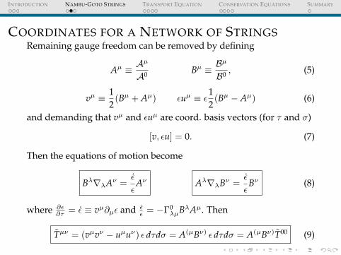
Given a network of many interacting strings, the energy density canbe used to form coarse-grained fields such as

Tµν = 〈A(µBν)〉 Fµν = 〈A[µBν]〉 (10)

One can show [Schubring, VV 2013] that

∇νTµν = 0 ∇νFµν = 0 (11)

For example, ∇νF0ν = 0 implies continuity of strings:

∇ · 〈u〉 = 0 (12)

The two conservation equations can also be rewritten as

∇ν〈AµBν〉 = 0 ∇ν〈BµAν〉 = 0 (13)

Note that these equations are exact since no assumptions were made.


DISTRIBUTION FUNCTIONI Conservation equations constrain the dynamics of string fluid

but do not describe evolution towards equilibrium.I In kinetic theory [VV 2013] one first derives a transport equation

for distribution f (A,B, x) defined on Ω2 ×M ≡ S2 × S2 ×M.I Then coarse-grained quantities are given by

〈Q〉(x) =∫

Q(A,B)f (A,B, x) dΩ2. (14)

I Energy densityρ(x) = 〈1〉 (15)

I Probability that random (A,B) rays are in a set X ⊆ Ω

p[(A,B) ∈ X] =1ρ

∫X

f (A,B)dΩ2 (16)

I For homogeneous eq. we make string chaos assumption [VV 2011]

p(A1,B1|A2,B2|...) ≈ p(A1,B1)p(A2,B2)... (17)

that can be justified both analytically [Schubring, VV 2013] andnumerically [Balma, Schubring, VV 2014].


LONGITUDINAL COLLISIONSWith the string chaos assumption longitudinal collisions give

f (A,B, t + ∆t) =∫

dΩ′2 f (A,B′, t)f (A′,B, t)ρ(t)

. (18)

Expanding to linear order in time,

∂f∂t

=1ρ

∫dΩ′2 Γ · [f (A,B′)f (A′,B)− f (A,B)f (A′,B′)]. (19)

where 1/Γ = ∆t is the equilibration time or correlation length.

σ

τ

B' B

B

B'' B' B

B(3) B'' B'

A'A

A

A A' A''

A A' A'' A(3) B


TRANSVERSE COLLISIONSI Transverse collisions will contribute to the energy density f (A,B)

with two terms similar to longitudinal terms.I So we just expect transverse collisions to add a contribution

Γ =1

∆t→ Γ =

1∆t

+ Γ⊥ (20)

whereΓ⊥ ∝ ρ|A ∧ B ∧ A′ ∧ B′|. (21)

I This can also be rewritten in terms of the three-velocities andtangent vectors of the interacting segments

Γ⊥ ∝ ρ|(v′ − v) · (u′ × u)|. (22)

I By denoting the proportionality constant as p (which may alsoinclude the inter-commutation probability if desired)

Γ =1

∆t+ pρ|A ∧ B′ ∧ A′ ∧ B|. (23)


H-THEOREM

I Then one can prove H-theorem for strings [VV 2013]

dHdt≤ 0 ≤ dS

dt, (24)

H(t) ≡∫

dΩ2f (A,B) log(f (A,B) ≡ −S(t) (25)

which a stringy version of the second law of thermodynamics.I One can also show [VV 2013] that the distribution relaxes to an

equilibrium state with independent statistics of A and B:

limt→∞

f (A,B, t) =1ρ

∫dΩ′2 f (A,B′)f (A′,B) (26)

orfeq(A,B) = fA(A)fB(B) (27)

I This allows a significant simplification of the conservationequation leading to a non-viscous string fluid dynamics.


INHOMOGENEOUS LIMIT

I Spatially homogenous transport equation trivially agrees with

∇ν〈AµBν〉 = 0 ∇ν〈BµAν〉 = 0 (28)

and the next step is to introduce spatial variations.I For example, one can derive an equation for f (A,B, x) by

considering motion of (A,B) segments with velocity v = A+B2 .

I This leads to the correct conservation of energy [VV 2013]

∂ρ

∂t+

∂

∂xk 〈vk〉 = 0, (29)

but does not respect the conservations of A and B fields,

∂

∂t〈Ai〉+

∂

∂xk 〈AiBk〉 = 0

∂

∂t〈Bi〉+

∂

∂xk 〈BiAk〉 = 0 (30)

I This is a real problem if one wants to use the transport equationto derive viscous string fluid equations.


TRANSPORT EQUATIONI The problem is that equations of motion imply that quantities Ai

move through space in the direction of B, and vise versa.I Then the correct difference equation [Schubring, VV 2103]

f (A,B, x, t + ∆t) =∫

dΩ′2 f (A,B′, x−B′∆t, t)f (A′,B, x− A′∆t, t)ρ−∇ · 〈v〉∆t

.

(31)and the spatial variations are described with an integral term(

∂f∂t

)spatial

= −1ρ

∫dΩ′2 f (A,B′)

←→∇ f (A′,B) (32)

where←→∇ ≡

←−∇ · B′ + A′ ·

−→∇ − 1

ρ∇ · 〈v〉 (33)

I This leads to the transport equation which gives rise toconservation equations in complete agreement with

∇ν〈AµBν〉 = 0 ∇ν〈BµAν〉 = 0 (34)


FRIEDMANN UNIVERSEI Friedmann metric in conformal coordinates

ds2 = a2(τ)(dτ 2 − dx2) (35)

whereH ≡ a/a is the Hubble constant.I Then the equations of motions

Bµ∂µAi = −H(Bi − (A · B)Ai) (36)

Aµ∂µBi = −H(Ai − (A · B)Bi). (37)and the change in energy density reduces to,

ε

ε= −H(1 + A · B). (38)

I After somewhat tedious calculations one can show that(∂f∂t

)gravitational

= H (∂A + ∂B − (1 + A · B)− 4A · B) f (39)

where∂A ≡ (B− (A · B)A) · ∂

∂A(40)


FLUID EQUATIONS

I To verify the conservation equation, we integrate thegravitational terms multiplied by a function Q(A,B):

H∫

Q(∂Af + ∂Bf ) dΩ2 −H〈Q(1 + A · B)〉 − 4H〈Q(A · B)〉 (41)

I After integrating by parts and some algebra this becomes,

−H〈∂AQ + ∂BQ〉 − H〈Q(1 + A · B)〉 (42)

I Choosing Q to be 1, Ai, Bi we obtain the gravitational correctionto the conservation equations,

∂ν〈vν〉 = −H〈1 + A · B〉 (43)

∂ν〈AiBν〉 = −2H〈vi〉 (44)

∂ν〈BiAν〉 = −2H〈vi〉 (45)

in full agreement with fluid approach [Schubring, VV 2013].


SUMMARY OF RESULTSDerived a transport equation in the homogeneous limit:

∂f∂t

=1ρ

∫dΩ′2 Γ · [f (A,B′)f (A′,B)− f (A,B)f (A′,B′)]

where Γ = 1∆t + pρ|A ∧ B′ ∧ A′ ∧ B| .

Proved an H-theorem and derived a local equilibrium distribution:

dHdt≤ 0 ⇔ feq(A,B) = fA(A)fB(B)

Constructed a correction to the transport eq. due to spatial variations:(∂f∂t

)spatial

= −1ρ

∫dΩ′2 f (A,B′)(

←−∇ · B′ + A′ ·

−→∇ − 1

ρ∇ · 〈v〉)f (A′,B).

Showed that gravitational terms are consistent with conservation eq.:(∂f∂t

)gravitational

= H (∂A + ∂B − (1 + A · B)− 4A · B) f

Documents

KINETIC THEORY OF STRINGS V U M HTTP://D UMN EDU …